Stabilised Inverse Flowline Evolution for Anisotropic Image Sharpening

Abstract

The central limit theorem suggests Gaussian convolution as a generic blur model for images. Since Gaussian convolution is equivalent to homogeneous diffusion filtering, one way to deblur such images is to diffuse them backwards in time. However, backward diffusion is highly ill-posed. Thus, it requires stabilisation in the model as well as highly sophisticated numerical algorithms. Moreover, sharpening is often only desired across image edges but not along them, since it may cause very irregular contours. This creates the need to model a stabilised anisotropic backward evolution and to devise an appropriate numerical algorithm for this ill-posed process.

We address both challenges. First we introduce stabilised inverse flowline evolution (SIFE) as an anisotropic image sharpening flow. Outside extrema, its partial differential equation (PDE) is backward parabolic in gradient direction. Interestingly, it is sufficient to stabilise it in extrema by imposing a zero flow there. We show that morphological derivatives – which are not common in the numerics of PDEs – are ideal for the numerical approximation of SIFE: They effortlessly approximate directional derivatives in gradient direction. Our scheme adapts one-sided morphological derivatives to the underlying image structure. It allows to progress in subpixel accuracy and enables us to prove stability properties. Our experiments show that SIFE allows nonflat steady states and outperforms other sharpening flows.

I Introduction

Image processing with evolution equations based on partial differential equations (PDEs) offers many successful tools with numerous applications, including image denoising [1], enhancement [2, 3], and variational restoration [4]. These methods are often inspired by physics. For instance, diffusion-based image processing takes its inspiration from the physical diffusion process. Its evolution equations are forward parabolic PDEs and have smoothing properties [3]. Conversely, diffusion backward in time has a sharpening effect. This can be useful for tasks such as contrast enhancement or deblurring, when no explicit blur kernel is known or blind deconvolution methods such as [5] are to be avoided. First image processing papers in this direction date back to 1955 [6]. Unfortunately, such processes are ill-posed: In the same way as forward diffusion attenuates high frequencies exponentially, backward diffusion amplifies them exponentially. Without additional stabilisation, the image range explodes within a short time. It took decades to come up with first successful solutions for this very difficult problem. A minimalistic regularisation to tame the explosive behaviour is pursued in stabilised inverse linear diffusion (SILD) [7]. It uses backward linear diffusion, but forbids over- and undershoots at extrema. Its sophisticated discretisation requires one-sided finite differences with minmod switches. Unfortunately, it sharpens not only across image edges, but also along them, which creates unpleasant irregular contours.

Contributions. The goal of our paper is build upon these ideas and improve them by introducing an anisotropic version of SILD. We advocate stabilised inverse flowline evolution (SIFE) as a novel PDE for image sharpening. Outside extrema, this filter is based on an anisotropic backward parabolic PDE in gradient direction. This anisotropy together with the ill-posedness of backward parabolic evolutions makes it very challenging to devise an adequate numerical algorithm. We show that by replacing finite differences with morphological derivatives, we can derive a scheme that is simple and elegant. We prove that it is stable w.r.t. a maximum–minimum principle. Thus, it cannot produce over- and undershoots. Our experiments show that SIFE allows nonflat steady states and performs better than SILD and shock filtering.

Related Work. In terms of image sharpening flows, our SIFE filter most closely resembles its predecessor SILD [7]. Both are backward parabolic, ill-posed, and benefit from a stabilisation at extrema. SILD, however, is linear and isotropic, while SIFE is nonlinear and anisotropic. Image analysis with PDEs that contain anisotropic backward parabolic terms have a long tradition [8, 9, 10], but they are typically stabilised by forward parabolic terms. Even with these stabilisations it remains nontrivial to find provably stable numerics. A backward parabolic 1-D model with range stabilisation and a simple explicit scheme has been introduced recently [11]. It is not applicable to our anisotropic 2-D problem. Shock filters [12, 13] are hyperbolic alternatives for morphological image sharpening. Their wave-like propagation is less challenging w.r.t. ill-posedness. To our knowledge, a fully backward parabolic 2-D anisotropic model has not been studied so far.

PDE-based processes are typically discretised with finite differences. This also includes shock filters and SILD. Due to its anisotropic and nonlinear nature, discretising SIFE with finite differences is numerically challenging. A specific feature of our numerical algorithm is its usage of morphological derivative approximations [14, 15, 16, 17]. So far, morphological derivatives are mainly used for feature detection. Apart from an image prior for denoising [18], we are not aware of any applications within implementations of PDE-based filters.

In recent years many deep learning approaches for image sharpening have been proposed [19]. They involve millions of hidden parameters and usually perform well without offering formal guarantees or deeper insights into their inner workings. Our goal is to come up with a transparent model with a single parameter, and to understand how to design provably stable numerical algorithms for it. Thus, comparing both complementary philosophies w.r.t. a single criterion such as performance or stability guarantees would not do justice to any of them. Both are needed, but under different requirements.

Paper Structure. Section II reviews the relevant background from mathematical morphology, in particular w.r.t. morphological derivatives. In Section III, we introduce SIFE and derive its numerical approximation with morphological derivatives. We compare the performance of SIFE with other image enhancing flows in Section IV. Section V offers conclusions and an outlook to future work.

II Review of Mathematical Morphology

Since morphological derivatives are essential for approximating the PDE-based SIFE filter, we first have to review necessary prerequisites from mathematical morphology.

II-A Dilation and Erosion

Mathematical morphology is a classical and very successful area of image processing [20]. Its building blocks are dilation and erosion. The dilation $\delta_{B}[f]$ of a continuous greyscale image $f$ with a structuring element $B$ – a set that typically characterises the notion of a neighbourhood – replaces each value of $f$ by its supremum within the structuring element. The erosion $\varepsilon_{B}[f]$ uses the infimum instead. Formally, the operations are defined as

$$\delta_{B}[f](\bm{x}) \;=\;\sup\,\{f(\bm{x}-\bm{b})\;|\;\bm{b}\in B\},$$ (1)

$$\varepsilon_{B}[f](\bm{x}) \;=\;\inf\,\{f(\bm{x}+\bm{b})\;|\;\bm{b}\in B\}.$$ (2)

In this paper, we only use ball-shaped structuring elements, i.e. symmetric intervals for 1-D signals, and disks for images. This guarantees rotation invariance and aligns morphological derivatives in gradient direction. In the following, we write $\delta_{r}$ and $\varepsilon_{r}$ for dilations and erosions with a ball of radius $r$.

It has been shown that dilation / erosion $u(\bm{x},t)$ of $f$ with a ball of radius $t$ solves the PDE

$$\partial_{t}u\;=\;\pm|\bm{\nabla}u|$$ (3)

with initial condition $u(\bm{x},0)=f(\bm{x})$; see e.g. [21]. Dilation uses the plus sign and erosion the minus sign. By $\bm{\nabla}$ we denote the spatial nabla operator, and $|\,.\,|$ is the Euclidean norm.

II-B Morphological Derivatives

Dilations and erosions allow morphological approximations of image derivatives. To this end, one computes differences between the original image, its dilations, and its erosions. For instance, the internal and external gradient [15, 16, 22] with a ball-shaped structuring element of radius $r$ are defined as

internal gradient: $$g_{r}^{-}[f](\bm{x})\; =\;\frac{f(\bm{x})-\varepsilon_{r}[f](\bm{x})}{r},$$ (4)

external gradient: $$g_{r}^{+}[f](\bm{x})\; =\;\frac{\delta_{r}[f](\bm{x})-f(\bm{x})}{r}.$$ (5)

Averaging both operators yields the Beucher gradient [14, 16].

Let us consider $f$ at some location $\bm{x}$ with nonvanishing gradient. It has been shown [22] that for $r\to 0$, the preceding morphological gradients converge to the derivative $f_{\eta}$ in flowline direction $\bm{\eta}=\frac{\bm{\nabla}f}{|\bm{\nabla}f|}$:

$$\lim_{r\to 0}\>g_{r}^{-}[f](\bm{x})\; =\;f_{\eta},$$ (6)

$$\lim_{r\to 0}\>g_{r}^{+}[f](\bm{x})\; =\;f_{\eta}.$$ (7)

Internal, external, and Beucher gradient show a structural resemblance to forward, backward, and central finite difference approximations of first order derivatives. For finite differences, we can construct approximations of higher order derivatives by computing the difference of approximations of lower order derivatives. This strategy is also applicable to morphological derivative approximations. For instance, the difference between internal and external gradient yields a morphological approximation of the second directional derivative $f_{\eta\eta}$ [17].

II-C Rouy–Tourin Scheme for PDE-based Morphology

For digital images, we need discrete analogues for dilation and erosion. One can directly discretise the set-theoretic description (1)–(2) by replacing the supremum with the maximum, and the infimum with the minimum. However, discretising the PDE (3) offers subpixel accuracy and an improved rotation invariance for small structuring elements. Therefore, we pursue the PDE-based approach in our paper.

For this purpose, we use the Rouy–Tourin upwind scheme [23]. For a derivation of this scheme from (1)–(2) with purely geometric arguments, we refer to van den Boomgaard [24]. Let $u_{i,j}^{k}$ denote the grey value of pixel $(i,j)$ at time level $k$, and assume that the pixel size is given by $h$, and the time step size by $\tau$. Then the Rouy–Tourin scheme approximates a dilation step with a disk of radius $\tau$ by

Initialising this iterative scheme with the original image $u^{0}_{i,j}=f_{i,j}$ and performing $k$ iterations approximates a dilation with a disk of radius $k\tau$. In 2D, one can show that this scheme satisfies the maximum–minimum principle

$$\min_{m,n}f_{n,m}\;\leq\;u_{i,j}^{k}\;\leq\;\max_{m,n}f_{n,m}\qquad\mbox{for all $i$, $j$}$$ (9)

provided that $\tau\leq\frac{h}{\sqrt{2}}$. In 1D, the time step step size limit is $\tau\leq h$. Analogously, erosion is approximated by

After this discussion of morphological concepts we are now in a position to study our novel PDE for image sharpening.

III Stabilised Inverse Flowline Evolution

In this section we introduce the stabilised inverse flowline evolution (SIFE) as a flow for image sharpening. It is motivated by the stabilised inverse linear diffusion (SILD) of Osher and Rudin [7]. However, while SILD is a linear and isotropic process that is approximated by finite differences, SIFE is nonlinear and anisotropic, and it benefits from morphological derivatives. First we derive the PDE for SIFE. Afterwards we propose a stable numerical algorithm with morphological derivatives in 1D, and we extend it to arbitrary dimensions.

III-A PDE Formulation of SIFE

Filters based on forward parabolic PDEs such as diffusion methods are widely used in image processing [1, 3]. For a continuous image $f(\bm{x})$, isotropic linear diffusion [1] creates a family $\,\{u(\bm{x},t)\>|\>t\geq 0\}\,$ of smoothed versions by solving

$$\partial_{t}u=\Delta u$$ (11)

with initial condition $u(\bm{x},0)=f(\bm{x})$ and reflecting boundary conditions. Here $\Delta$ denotes the spatial Laplacian. The smoothness increases with the diffusion time $t$.

While forward diffusion has smoothing properties, backward diffusion sharpens images by reversing smoothing. In contrast to forward parabolic processes, backward parabolic evolutions are typically ill-posed and need a stabilisation to avoid instabilities such as the violation of a maximum–minimum principle.

Osher and Rudin proposed such a stabilisation. Their stabilised inverse linear diffusion (SILD) [7] regularises backward diffusion by fixing values at extrema:

$$\partial_{t}u\;=\;-\mbox{sgn}(|\bm{\nabla}u|)\,\Delta u\,.$$ (12)

The sign factor implements the stabilisation, since $|\bm{\nabla}u|$ vanishes in extrema. This enforces a maximum–minimum principle. SILD has one obvious drawback: For image sharpening, one is usually only interested in sharpening across edges, but not along them. The latter can cause unpleasant irregular contours. Being an isotropic process, however, SILD does not allow such a direction-specific filtering.

As a remedy, we propose an anisotropic modification of SILD that acts only perpendicular to edges, i.e. in flowline direction $\bm{\eta}=\frac{\bm{\nabla}u}{|\bm{\nabla}u|}$. This leads to the equation

$$\partial_{t}u\;=\;-\mbox{sgn}(|\bm{\nabla}u|)\,\partial_{\eta\eta}u$$ (13)

which we call stabilised inverse flowline evolution (SIFE). Note that unlike SILD, SIFE is nonlinear, since $\bm{\eta}$ depends on the evolving local image structure $u(\bm{x},t)$.

III-B Numerical Challenges of SIFE

While it is easy to write down the SIFE PDE, finding stable algorithms is very challenging for two reasons:

1. Equation (13) is backward parabolic and hence ill-posed. Thus, naive discretisations immediately create instabilities. As a remedy, we will adapt the sophisticated minmod scheme for SILD [7] to our purpose.

2. The anisotropy poses additional problems. A classical way to handle it would be to use

   $$u_{\eta\eta}\;=\;\frac{u_{x}^{2}\,u_{xx}\>+\>2\,u_{x}\>u_{y}\>u_{xy}\>+\;u_{y}^{2}\,u_{yy}}{u_{x}^{2}\>+\>u_{y}^{2}}$$ (14)

   and approximate all derivatives on the right-hand side with finite differences. Unfortunately, it is completely unclear how this can be combined with the minmod concept of SILD. Here, morphological derivatives can rescue us, since they effortlessly approximate derivatives in flowline direction in any dimension.

We now proceed with these ideas by first translating the SILD numerics based on finite differences into a stable SIFE scheme with morphological derivatives. This is done in the 1-D setting, where we also prove stability results. Afterwards we generalise the morphological scheme to higher dimensions.

III-C Morphological SIFE Numerics in 1D

In 1D, the minmod finite difference scheme for SILD [7] is given by

with initial condition $\bm{u}^{0}=\bm{f}$. To implement reflecting boundary conditions, the discrete image is extended by a mirrored boundary layer of size two pixels. The minmod function $\mathsf{mm}$ returns the argument with the smallest absolute value if all of them have equal sign, and $0$ otherwise. In extrema, forward and backward differences have different signs, such that the minmod function yields zero. Hence, grey values of extrema are frozen in time. This is essential for the stability of the discrete evolution.

To transfer this stabilisation concept to SIFE in arbitrary dimensions, we replace finite differences by morphological derivatives. This yields simple approximations of the directional derivative $\partial_{\eta\eta}u$. We start with the 1-D case.

For a 1-D signal, we propose the following morphological scheme for SIFE:

with reflecting boundaries and the initial signal $\bm{u}^{0}=\bm{f}$. The operations $\delta_{r}$ and $\varepsilon_{r}$ denote 1-D dilation and erosion with a symmetric 1-D structuring element. Since morphological first order derivatives approximate $u_{\eta}=|\bm{\nabla}u|$, they are always nonnegative. Thus, the minmod becomes the minimum. In (16), we need dilations and erosions with radii $r$ and $2r$. We compute them with the Rouy–Tourin scheme (8), (10). Its stability condition restricts us to radii of $r\leq h$ in 1D. However, if one aims at accurate derivative approximations, small radii should be used. Thus, we recommend $r:=\frac{h}{2}$ and use this throughout our experiments. We perform one iteration for $\varepsilon_{r}$ and $\delta_{r}$, and two for $\varepsilon_{2r}$ and $\delta_{2r}$.

It is not hard to see that outside extrema the SIFE scheme approximates its underlying PDE with first order consistency in space and time. In extrema it reproduces the continuous model exactly by preventing any changes. This also implies that the continuous SIFE model and its algorithm do not alter binary images, since they only consist of extrema and already offer maximal sharpness.

III-D Stability of the 1-D SIFE Scheme

For a disk radius $r=h$, SIFE is equivalent to SILD in 1D. Thus, it is not surprising that SIFE offers the same stability properties that have been claimed for SILD in 1D. However, no proof for SILD is given in [7], and establishing stability results also for $r<h$ – which is relevant for us – is technically more demanding. Below is our stability theorem. Since a detailed proof is very lengthy, we only sketch the main steps.

Theorem 1 (Stability of SIFE)

Let $\bm{f}$ be a discrete 1-D signal and $r\leq h$. Consider the SIFE scheme (16) with one Rouy–Tourin iteration for $\delta_{r}$ and $\varepsilon_{r}$, and two for $\delta_{2r}$ and $\varepsilon_{2r}$. If $\tau\leq r^{2}$, the following properties hold for all $k\geq 0$:

1. Preservation of Monotonicity

   $$f_{i-1}\leq f_{i}\quad\forall i\quad\Rightarrow\quad u^{k}_{i-1}\leq u^{k}_{i}\quad\forall i,$$ (17)

   $$f_{i-1}\geq f_{i}\quad\forall i\quad\Rightarrow\quad u^{k}_{i-1}\geq u^{k}_{i}\quad\forall i.$$ (18)

2. Maximum–minimum Principle

   $$\min_{j}f_{j}\;\leq\;u_{i}^{k}\;\leq\;\max_{j}f_{j}\quad\forall i.$$ (19)

Sketch of the Proof. First we prove monotonicity preservation. Let $\bm{u}^{k}$ be locally concave and increasing (other cases can be treated in a similar way). Thus, we have $u^{k}_{i+1}-u^{k}_{i}\leq u^{k}_{i}-u^{k}_{i-1}$ and $u_{i-1}^{k}\leq u_{i}^{k}$. Then the Rouy–Tourin dilations and erosions in (16) yield

$$\delta_{2r}[u]_{i}^{k} \,=\,u_{i}^{k}+\frac{2r}{h}(u_{i+1}^{k}-u_{i}^{k})+\frac{r^{2}}{h^{2}}(u_{i+2}^{k}-2u_{i+1}^{k}+u_{i}^{k}),$$

$$\delta_{r}[u]_{i}^{k} \,=\,u_{i}^{k}+\frac{r}{h}(u_{i+1}^{k}-u_{i}^{k}),$$

$$\varepsilon_{r}[u]_{i}^{k} \,=\,u_{i}^{k}-\frac{r}{h}(u_{i}^{k}-u_{i-1}^{k}),$$

$$\varepsilon_{2r}[u]_{i}^{k} \,=\,u_{i}^{k}-\frac{2r}{h}(u_{i}^{k}-u_{i-1}^{k})+\frac{r^{2}}{h^{2}}(u_{i-2}^{k}-2u_{i-1}^{k}+u_{i}^{k}).$$

This gives the differences

$$\delta_{2r}[u]_{i}^{k}-\delta_{r}[u]_{i}^{k} \;\leq\;\delta_{r}[u]_{i}^{k}-u_{i}^{k}\;\leq\;u_{i}^{k}-\varepsilon_{r}[u]_{i}^{k},$$

$$\delta_{r}[u]_{i}^{k}-u_{i}^{k} \;\leq\;u_{i}^{k}-\varepsilon_{r}[u]_{i}^{k}\;\leq\;\varepsilon_{r}[u]_{i}^{k}-\varepsilon_{2r}[u]_{i}^{k}.$$

With that, SIFE results in

$$u^{k+1}_{i}\>=\>u_{i}^{k}-\tau\,\frac{\delta_{2r}[u]_{i}^{k}-2\delta_{r}[u]_{i}^{k}+u_{i}^{k}}{r^{2}}\,.$$

Since we also assume concavity of $\bm{u}^{k}$ in $i-1$, we get

$$u^{k+1}_{i-1}\>=\>u_{i-1}^{k}-\tau\,\frac{\delta_{2r}[u]_{i-1}^{k}-2\delta_{r}[u]_{i-1}^{k}+u_{i-1}^{k}}{r^{2}}\,.$$

Subtracting both equations gives

$$u^{k+1}_{i}-u^{k+1}_{i-1} \;=\;(u_{i}^{k}-u^{k}_{i-1})\Big{(}1-\frac{\tau}{r^{2}}\Big{)}$$ (20)

$$\;-\;\frac{\tau}{r^{2}}(\delta_{2r}[u]_{i}^{k}-\delta_{2r}[u]_{i-1}^{k})$$

$$\;+\;\frac{2\tau}{r^{2}}(\delta_{r}[u]_{i}^{k}-\delta_{r}[u]_{i-1}^{k}).$$

In a next step one shows that

$$\delta_{2r}[u]_{i}^{k}-\delta_{2r}[u]_{i-1}^{k}\;\leq\;\delta_{r}[u]_{i}^{k}-\delta_{r}[u]_{i-1}^{k}$$ (21)

holds by plugging in the results for dilation and erosion, and exploiting the local concavity of $\bm{u}^{k}$ together with $r\leq h$. Plugging (21) in (20), we obtain

$$u^{k+1}_{i}-u^{k+1}_{i-1} \;\geq\;(u_{i}^{k}-u^{k}_{i-1})\Big{(}1-\frac{\tau}{r^{2}}\Big{)}$$

$$\;\quad\;+\frac{\tau}{r^{2}}\,(\delta_{r}[u]_{i}^{k}-\delta_{r}[u]_{i-1}^{k})$$

$$\;\geq\;0\,,$$

since $\bm{u}^{k}$ and $\delta_{r}[\bm{u}^{k}]$ are increasing and $\tau\leq r^{2}$. Therefore, monotonicity is preserved in this case.

If $\bm{u}^{k}$ has a maximum in $i$, then SIFE results in

$$u^{k+1}_{i} \>=\>u_{i}^{k},$$

$$u^{k+1}_{i-1} \>=\>u_{i-1}^{k}+\tau\,\frac{\delta_{r}[u]_{i-1}^{k}+u_{i-1}^{k}}{r^{2}}.$$

The difference between the two equations yields

$$u^{k+1}_{i}-u^{k+1}_{i-1}\>=\;(u_{i}^{k}-u^{k}_{i-1})-\tau\frac{\delta_{r}[u]_{i-1}^{k}+u_{i-1}^{k}}{r^{2}}\>\geq\>0$$

for $\tau\leq r^{2}$, since $\delta_{r}[u]_{i-1}^{k}\leq u_{i}^{k}$ if $\bm{u}^{k}$ has a maximum in $i$. Thus, the monotonicity is preserved in the increasing case. The decreasing case in analogous.

Monotonicity preservation implies the maximum–minimum principle: Extrema are not changed by the evolution, and monotone regions remain monotone. Therefore, values cannot increase past maxima or decrease below minima.   $\square$

III-E Morphological SIFE Numerics in Higher Dimensions

The extension of the SIFE scheme to higher dimensions is straightforward: One simply needs to use a higher dimensional, ball-shaped structuring element, e.g. a disk in case of an image. The stability limit of the Rouy-Tourin scheme restricts us to radii $\,r\leq h/\sqrt{2}\,$ in 2D. Also in 2D we recommend $r=h/2$, a single Rouy–Tourin iteration for $\varepsilon_{r}$ and $\delta_{r}$, and two iterations for $\varepsilon_{2r}$ and $\delta_{2r}$. This offers a good compromise between subpixel accuracy and efficiency.

Interestingly, in our experiments the 2-D SIFE scheme satisfies a maximum–minimum principle for time step sizes up to $r^{2}$. Thus, its stability limit does not deteriorate when going from 1D to 2D. This is uncommon for explicit discretisations of PDE-based methods. SILD, for instance, must reduce its stability limit from $\tau\leq\frac{h^{2}}{2}$ to $\tau\leq\frac{h^{2}}{4}$ [7]. However, in contrast to SILD, the extreme anisotropy of SIFE turns it into a pure 1-D sharpening flow: It only acts in flowline direction. If this is the reason why its 1-D stability limit transfers to higher dimensions without further restrictions, also stability reasonings favour SIFE over SILD.

IV Experiments

Let us now evaluate the performance of SIFE by comparing it to two PDE evolutions that have been designed for the same purpose: SILD and shock filtering. A widely used shock filter [12, 13] is governed by the hyperbolic evolution

$$\partial_{t}u=-\mbox{sgn}(\Delta u)|\bm{\nabla}u|$$ (22)

with initial condition $u(\bm{x},0)=f(\bm{x})$ and reflecting boundary conditions. The sign of $\Delta u$ signals whether we are in the influence zone of a maximum $(\Delta u<0)$ or a minimum $(\Delta u>0)$. This determines if we perform dilation or erosion. Shocks develop at the interface between adjacent influence zones.

For our experiments, we discretise the shock filter with the Rouy–Tourin scheme. Our grid size $h$ is assumed to be $1$. For the morphological derivatives in SIFE we choose a disk of radius $r=0.5$ as structuring element. This subpixel accuracy is achieved with a single Rouy–Tourin step. For SIFE and SILD we use the time step size $\tau=0.2$, and for shock filtering $\tau=0.5$.

In Figure 1, we compare the steady states ($t\to\infty$) of SIFE, SILD, and shock filtering. While all approaches produce nonflat steady states with piecewise constant segmentations, they differ substantially in detail. This is best visible in the zooms in Figure 2.

Interestingly, the backward parabolic SILD and SIFE processes produce more regular edges than the hyperbolic shock filter. We conjecture that this is caused by the fact that SILD and SIFE employ a $5\times 5$ stencil to approximate a second order differential operator with first order accuracy. The minmod or minimum switches aim at small absolute derivative approximations, which is needed for regularising the ill-posed backward parabolic evolution. The hyperbolic shock filter, however, can be discretised adequately within a $3\times 3$ neighbourhood. It is steered by a conventional $5$-point stencil that approximates the Laplacian with second order accuracy.

From a practical perspective, the more regular boundary structure of SILD and SIFE makes these backward parabolic sharpenings preferable over the hyperbolic shock filter. This demonstrates that backward parabolic evolutions deserve more attention than the more widely used hyperbolic processes.

It should be noted that SIFE has the most pleasant edge structure due to the absense of a backward parabolic term along edges: Its anisotropy allows to sharpen only across edges (i.e. in gradient direction $\bm{\eta}$). In contrast, the isotropic sharpening of SILD causes irregular edges, since backward parabolic evolution along edges is not prevented. This is also in agreement with Haralick’s observations in the context of edge detection [25], where he argues that $u_{\eta\eta}$ should be favoured over $\Delta u$. In conclusion, Figures 1–2 show that the SIFE model and its algorithmic implementation do exactly what they have been designed for.

If we aim at image sharpening rather than a piecewise constant segmentation-like result, we should stop the evolution at a finite time. This is illustrated in Figure 3 where SIFE nicely sharpens the Gaussian-blurred test image pepper without introducing staircasing artefacts. The runtime for processing this $512\times 512$ image with 50 iterations on a Computer with Intel^© Core™  i9-11900K CPU @ 3.50 GHz is 0.3 seconds.

original	shock filter
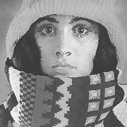
SILD	SIFE

Figure 1: Comparison of the steady states of shock filtering, SILD, and SIFE for the $256\times 256$ greyscale image trui.

shock filter	SILD	SIFE

Figure 2: Zoom into a $54\times 64$ window of Figure 1.

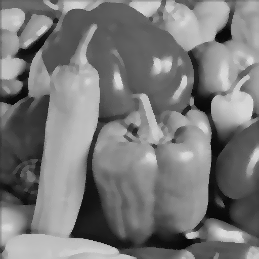
blurred image	sharpened image, $t=10$

Figure 3: Image sharpening with SIFE. The original $512\times 512$ peppers image was degraded with Gaussian blur with $\sigma=3$.

V Conclusions

We have proposed stabilised inverse flowline evolution (SIFE) as a novel image sharpening flow. It is goverend by an anisotropic backward parabolic PDE in gradient direction that is stabilised at extrema. Thus, its sharpening direction varies from location to location, which makes the design of numerical algorithms challenging. For its discretisation, morphological derivatives provide simple and elegant approximations of the directional derivative in gradient direction. Our experiments show that this filter can outperform other PDE-based processes for image sharpening such as stabilised inverse linear diffusion and shock filtering.

In a more general setting, we have seen how one can handle ill-posed nonlinear, and anisotropic backward parabolic PDEs in a numerically adequate way. Thus, if such processes appear interesting from a modelling perspective, there is no reason to shy away from them. Moreover, our contributions may go far beyond concrete sharpening applications: It is very common to express PDE-based methods in their gauge coordinates $\bm{\eta}\parallel\bm{\nabla}u$ and $\bm{\xi}\perp\bm{\nabla}u$, e.g. in the context of level set methods and active contour models. Any progress on appropriate discretisations for differential operators of type $\,a\,\partial_{\eta\eta}+b\,\partial_{\xi\xi}$, where $a$ and $b$ may have any sign, is immediately applicable to all these problems. Our ongoing research is exploring extensions of SIFE towards this general formulation and other applications.

To the best of our knowledge, our work is the first to explore the potential of morphological derivatives for numerical analysis: It shows that morphological derivatives are ideal tools to approximate PDEs with derivatives in gradient direction. Moreover, it is natural to combine them with advanced numerical ideas such as adaptive one-sided approximations. This may also pave the path for applications beyond image analysis, e.g. in computational fluid mechanics where upwinding, minmod schemes, and WENO approximations are popular.

Acknowledgement. We thank Tobias Alt for useful comments on a draft version of this paper.

References

- [1] T. Iijima, “Basic theory on normalization of pattern (in case of typical one-dimensional pattern),” Bulletin of the Electrotechnical Laboratory, vol. 26, pp. 368–388, 1962, in Japanese.
- [2] P. Perona and J. Malik, “Scale space and edge detection using anisotropic diffusion,” IEEE Transactions on Pattern Analysis and Machine Intelligence, vol. 12, pp. 629–639, 1990.
- [3] J. Weickert, Anisotropic Diffusion in Image Processing. Stuttgart: Teubner, 1998.
- [4] G. Aubert and P. Kornprobst, Mathematical Problems in Image Processing: Partial Differential Equations and the Calculus of Variations, 2nd ed., ser. Applied Mathematical Sciences. New York: Springer, 2006, vol. 147.
- [5] Y. Bai, G. Cheung, X. Liu, and W. Gao, “Graph-based blind image deblurring from a single photograph,” IEEE Transactions on Image Processing, vol. 28, no. 3, pp. 1404–1418, Mar. 2019.
- [6] L. S. G. Kovasznay and H. M. Joseph, “Image processing,” Proceedings of the IRE, vol. 43, no. 5, pp. 560–570, May 1955.
- [7] S. Osher and L. Rudin, “Shocks and other nonlinear filtering applied to image processing,” in Applications of Digital Image Processing XIV, ser. Proceedings of SPIE, A. G. Tescher, Ed. Bellingham: SPIE Press, 1991, vol. 1567, pp. 414–431.
- [8] D. Gabor, “Information theory in electron microscopy,” Laboratory Investigation, vol. 14, pp. 801–807, 1965.
- [9] G. Gilboa, N. A. Sochen, and Y. Y. Zeevi, “Forward-and-backward diffusion processes for adaptive image enhancement and denoising,” IEEE Transactions on Image Processing, vol. 11, no. 7, pp. 689–703, 2002.
- [10] M. Welk and J. Weickert, “PDE evolutions for M-smoothers in one, two, and three dimensions,” Journal of Mathematical Imaging and Vision, vol. 63, pp. 157–185, Feb. 2021.
- [11] L. Bergerhoff, M. Cárdenas, J. Weickert, and M. Welk, “Stable backward diffusion models that minimise convex energies,” Journal of Mathematical Imaging and Vision, vol. 62, no. 6–7, pp. 941–960, Jul. 2020.
- [12] H. P. Kramer and J. B. Bruckner, “Iterations of a non-linear transformation for enhancement of digital images,” Pattern Recognition, vol. 7, pp. 53–58, 1975.
- [13] S. Osher and L. I. Rudin, “Feature-oriented image enhancement using shock filters,” SIAM Journal on Numerical Analysis, vol. 27, pp. 919–940, 1990.
- [14] S. Beucher, “Segmentation d’images et morphologie mathématique,” Ph.D. dissertation, Ecole des Mines de Paris, Jun. 1990.
- [15] J. Lee, R. Haralick, and L. Shapiro, “Morphologic edge detection,” IEEE Journal on Robotics and Automation, vol. 3, no. 2, pp. 142–156, Apr. 1987.
- [16] J. F. Rivest, P. Soille, and S. Beucher, “Morphological gradients,” Journal of Electronic Imaging, vol. 2, no. 4, pp. 2–11, Oct. 1993.
- [17] L. J. van Vliet, I. T. Young, and G. L. Beckers, “A nonlinear Laplace operator as edge detector in noisy images,” Computer Vision, Graphics, and Image Processing, vol. 45, no. 2, pp. 167–195, Feb. 1989.
- [18] M. Nakashizuka, “Image regularization with higher-order morphological gradients,” in 23rd European Signal Processing Conference (EUSIPCO), Sep. 2015, pp. 1820–1824.
- [19] K. Zhang, W. Ren, W. Luo, W. Lai, B. Stenger, M. Yang, and H. Li, “Deep image deblurring: A survey,” International Journal of Computer Vision, in press.
- [20] P. Soille, Morphological Image Analysis, 2nd ed. Berlin: Springer, 2004.
- [21] R. W. Brockett and P. Maragos, “Evolution equations for continuous-scale morphology,” in Proc. IEEE International Conference on Acoustics, Speech and Signal Processing, vol. 3, San Francisco, CA, Mar. 1992, pp. 125–128.
- [22] P. Maragos, “Morphological filtering for image enhancement and feature detection,” in Image and Video Processing Handbook, A. C. Bovik, Ed. Orlando: Elsevier, 2005, pp. 135–156.
- [23] E. Rouy and A. Tourin, “A viscosity solutions approach to shape-from-shading,” SIAM Journal on Numerical Analysis, vol. 29, no. 3, pp. 867–884, Jul. 1992.
- [24] R. van den Boomgaard, “Numerical solution schemes for continuous-scale morphology,” in Scale-Space Theories in Computer Vision, ser. Lecture Notes in Computer Science, M. Nielsen, P. Johansen, O. F. Olsen, and J. Weickert, Eds. Berlin: Springer, 1999, vol. 1682, pp. 199–210.
- [25] R. M. Haralick, “Digital step edges from zero crossing of second directional derivatives,” IEEE Transactions on Pattern Analysis and Machine Intelligence, vol. 6, no. 1, pp. 58–68, Jan. 1984.