Rectifying Open-set Object Detection:
A Taxonomy, Practical Applications, and Proper Evaluation

Abstract

Open-set object detection (OSOD) has recently gained attention. It is to detect unknown objects while correctly detecting known objects. In this paper, we first point out that the recent studies’ formalization of OSOD, which generalizes open-set recognition (OSR) and thus considers an unlimited variety of unknown objects, has a fundamental issue. This issue emerges from the difference between image classification and object detection, making it hard to evaluate OSOD methods’ performance properly. We then introduce a novel scenario of OSOD, which considers known and unknown classes within a specified super-class of object classes. This new scenario has practical applications and is free from the above issue, enabling proper evaluation of OSOD performance and probably making the problem more manageable. Finally, we experimentally evaluate existing OSOD methods with the new scenario using multiple datasets, showing that the current state-of-the-art OSOD methods attain limited performance similar to a simple baseline method. The paper also presents a taxonomy of OSOD that clarifies different problem formalizations. We hope our study helps the community reconsider OSOD problems and progress in the right direction.

1 Introduction

Open-set object detection (OSOD) is the problem of correctly detecting known objects in images while adequately dealing with unknown objects (e.g., detecting them as unknown). Here, known objects are the class of objects that detectors have seen at training time, and unknown objects are those they have not seen before. It has attracted much attention recently [25, 6, 18, 15, 32, 16, 42].

Early studies [25, 24, 6] consider how accurately detectors can detect known objects, without being distracted by unknown objects present in input images. We refer to this as OSOD-I in this paper. Recent studies [18, 15, 32, 16, 42] have shifted the focus to detecting unknown objects as well. They follow the studies of open-set recognition (OSR) [29, 2, 26, 27, 35, 43], which aims at detecting images of any arbitrary classes that the classifier has not seen before. Specifically, the recent OSOD studies attempt to develop a method that can detect unknown-class objects as such while detecting known-class objects accurately. We will refer to this as OSOD-II.

Table 1: Proposed categorization of OSOD problems. “Det. target” indicates the target of detection. K and U indicate known and unknown objects, respectively.

Type	Det. target	Unknown	Evaluation
OSOD-I[25, 6]	K	Any classes	Feasible
OSOD-II[18, 16]	K+U	Any classes	Hard
OSOD-III	K+U	Any sub-classes in a known super-class	Feasible

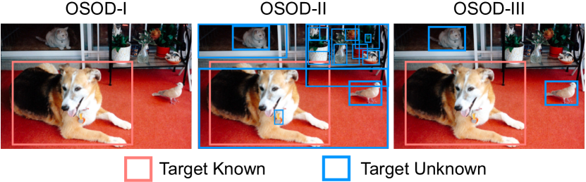
Figure 1: Illustration of OSOD-I, II, and III. OSOD-I: The interest is in detecting known objects without being distracted by unknown objects. OSOD-II: The interest is in detecting known and unknown objects as such. OSOD-III: The interest is in detecting known and unknown objects belonging to the same super-class as such.

In this paper, we show that OSOD-II, defined above, is ill-posed. Why? We want our detector to detect unknown-class objects in addition to known-class objects. Then, since this is a detection task, our detector must be fully aware of what to detect and what not at inference time. However, we cannot make this happen since unknown-class objects belong to an open set; they can be any arbitrary classes. A reconciliation is to make our detector detect any “objects” appearing in images, classifying them as either known or unknown classes. However, this may not be feasible since it is unclear what are “objects.” For example, are tires of a car objects? Note that such a difficulty does not occur with OSR since it considers classification, not detection. Second, it is hard to evaluate the performance of methods for OSOD-II. Following the studies of OSOD-I [25, 6], the previous studies employ A-OSE [25] and WI [6] to evaluate methods’ performance. However, they are basically the metrics for measuring the accuracy of known object detection; they cannot measure that of unknown object detection.

What was also overlooked in previous studies is the applications of OSOD. Apart from the above issues, OSOD-II (i.e., detecting any unseen objects)

may have few practical applications, while it is scientifically intriguing. Considering these, we introduce a more practical scenario of OSOD, which we name OSOD-III. It differs from OSOD-II in the definition of unknown classes. Specifically, OSOD-III considers only unknown classes belonging to the same super-classes as known classes. Figure. 1 and Table 1 briefly demonstrate the concept of OSOD-III. Example applications are as follows.

• For a smartphone app detecting and recognizing animal species, we want the app to detect new animal species that the app’s detector has not learned while running. (The super-class is animal species.)

• For an ADAS (advanced driver-assistance system) detecting traffic signs, we want the system to detect unseen traffic signs in remote areas with insufficient training data. (The super-class is traffic signs.)

Once unknown-class objects are detected, it is notified to a higher-level entity, for example, the system administrators, who may want to update the detectors by collecting training data and retraining them.

Owing to the difference in the definition of unknown classes, OSOD-III is free from the issue of OSOD-II. We can identify what the detectors should detect and what not. This also enables the precise evaluation of methods. Object detection has the inherent trade-off between precision and recall. The standard metric for object detection is AP (average precision), i.e., an AUC (area under the curve) metric independent of the operating point of detectors. Owing to the above formulation, we can use AP not only for known object detection but for unknown object detection.

Based on the above, we evaluate the performance of existing OSOD methods on OSOD-III problems. Existing OSOD methods, all designed assuming OSOD-II, are fortunately applicable to OSOD-III problems with little or no modification. Note that OSOD-III’s formalization enables, for the first time, the precise evaluation of OSOD methods’ performance with AP for unknown object detection. Toward this end, we design benchmark tests that simulate real-world problems categorized as OSOD-III using three datasets, Open Images [20], Caltech-UCSD Birds-200-2011 (CUB200) [37], and Mapillary Traffic Sign Dataset (MTSD) [8]. We then evaluate three state-of-the-art OSOD methods, i.e., ORE [18], VOS [7], and OpenDet [16]. For comparison, we also consider a naive baseline that classifies predicted boxes as known or unknown based on a simple uncertainty measure computed from predicted class scores.

The results show that existing methods, including the baseline method, do not necessarily perform well. First, no method generally achieves the necessary level of performance for practical applications. Second, the existing methods, which show good performance in the previous studies’ metrics, i.e., A-OSE and WI, are on par or even worse than our baseline in the unknown detection AP. Notably, the baseline uses standard detectors trained normally and does not employ an extra training step or an additional architecture. Thus, we conclude that there is currently no method achieving satisfactory performance in practical use and that further improvement is needed.

Table 2: The class split employed in the standard benchmark test employed in recent studies of OSOD [18, 15, 16, 41, 42, 38]. Split 1 consists of 20 PASCAL VOC classes. Split 2, 3, and 4 consist of all the COCO classes but those of Split 1. A typical setting is to use Split 1 as known categories and Split 2-4 as unknown categories. Note the dissimilarity between the known and unknown categories.

	Split 1	Split 2	Split 3	Split 4
Classes	PASCAL VOC objects (20)	Outdoor(5), Accessories(5), Appliance(5), Animal(4), Truck	Sports(10), Food(10)	Electronic(5), Indoor(7), Kitchen(6), Furniture(2)

2 Rethinking Open-set Object Detection

2.1 Formalizing Problems

We first formalize the problem of open-set object detection (OSOD). Previous studies refer to two different problems as OSOD without clarification. We use the names of OSOD-I and -II to distinguish the two, which are defined as follows.

OSOD-I   The goal is to detect all instances of known objects in an image without being distracted by unknown objects present in the image. We want to avoid mistakenly detecting unknown object instances as known objects.

OSOD-II  The goal is to detect all instances of known and unknown objects in an image, identifying them correctly (i.e., classifying them to known classes if known and to the “unknown” class otherwise).

OSOD-I and -II both consider applying a closed-set object detector (i.e., a detector trained on a closed-set of object classes) to an open-set environment where the detector encounters objects of unknown class. Their difference is whether or not the detector detects unknown objects. OSOD-I does not; its concern is with the accuracy of detecting known objects. This problem is first studied in [6, 24, 25]. On the other hand, OSOD-II detector detects unknown objects as well, and thus their detection accuracy matters. OSOD-II is often considered as a part of open-world object detection (OWOD) [18, 15, 41, 32, 38].

2.2 Ill-posedness of OSOD-II

The existing studies of OSOD-II rely on OWOD [18] for the problem formalization, which aims to generalize the concept of OSR (open-set recognition) to object detection. In OSR, unknown means “anything but known”. Its direct translation to object detection is that any arbitrary classes of objects but known objects can be considered unknown. This formalization is reflected in the experimental settings employed in these studies. Table 2 shows the setting, which treats the 20 object classes of PASCAL VOC [9] as known classes and non-overlapping 60 classes from 80 of COCO [21] as unknown classes. This class split indicates the basic assumption that there is little relation between known and unknown objects.

However, this OSOD-II’s formalization has an issue, making it ill-posed. It is because the task is detection. Detectors are requested to detect only objects that should be detected. It is a primary problem of object detection to judge whether or not something should be detected. What should not be detected include objects belonging to the background and irrelevant classes. Detectors learn to make this judgment, which is feasible for a closed set of object classes; what to detect is specified. However, this does not apply to OSOD-II, which aims at detecting also unknown objects defined as above. It is infeasible to specify what to detect and what not for any arbitrary objects in advance.

A naive solution to this difficulty is to detect any objects as long as they are “objects.” However, it is not practical since defining what an object is itself hard. Figure 2 provides examples from COCO images. COCO covers only 80 object classes (shown in red rectangles in the images), and many unannotated objects are in the images (shown in blue rectangles). Is it necessary to consider every one of them? Moreover, it is sometimes subjective to determine what constitutes individual “objects.” For instance, a car consists of multiple parts, such as wheels, side mirrors, and headlights, which we may want to treat as “objects” depending on applications. This difficulty is well recognized in the prior studies of open-world detection [18, 15] and zero-shot detection [1, 23].

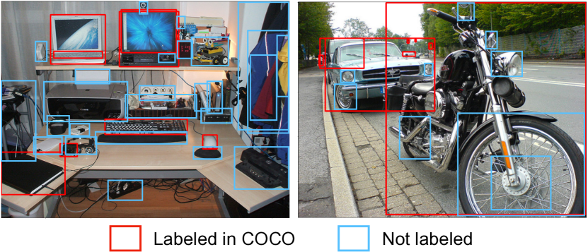
Figure 2: Example images showing that “object” is an ambiguous concept. It is impractical to cover an unlimited range of object instances with a finite set of predefined categories.

2.3 Metrics for Measuring OSOD Performance

The above difficulty also leads to make it hard to evaluate how well detectors detect unknown objects. The previous studies of OSOD employ two metrics for evaluating methods’ performance, i.e., absolute open-set error (A-OSE) [25] and wilderness impact (WI) [6]. A-OSE is the number of predicted boxes that are in reality unknown objects but wrongly classified as known classes [25]. WI measures the ratio of the number of erroneous detections of unknowns as knowns (i.e., A-OSE) to the total number of detections of known instances, given by

$${\rm WI}=\frac{P_{K}}{P_{K\cup U}}–1=\frac{\rm{A\text{-}OSE}}{\mathrm{TP}_{\mathit{known}}+\mathrm{FP}_{\mathit{known}}},$$ (1)

where $P_{K}$ indicates the precision measured in the close-set setting; $P_{K\cup U}$ is that measured in the open-set setting; and $\mathrm{TP}_{\mathit{known}}$ and $\mathrm{FP}_{\mathit{known}}$ are the number of true positives and false positives for known classes, respectively.

These two metrics are originally designed for OSOD-I; they evaluate detectors’ performance in open-set environments. Precisely, they measure how frequently a detector wrongly detects and misclassifies unknown objects as known classes (lower is better).

Nevertheless, previous studies of OSOD-II have employed A-OSE and WI as primary performance metrics. We point out that these metrics are pretty insufficient to evaluate OSOD-II detectors since they cannot evaluate the accuracy of detecting unknown objects, as mentioned above. They evaluate only one type of error, i.e., detecting unknown as known, and ignore the other type of error, detecting known as unknown.

In addition, we point out that A-OSE and WI are not flawless even as OSOD-I performance metrics. That is, they merely measure the detectors’ performance at a single operating point; they cannot take the precision-recall tradeoff into account, the fundamental nature of detection. Specifically, previous studies [18] report A-OSE values for bounding boxes with confidence score $\geq 0.05$. As for WI, previous studies [18, 15, 16, 32] choose the operating point of recall $=0.8$. Thus, they show performance only partially since the setting is left to end users. Figures 3(a) and (b) show the profiles of A-OSE and WI, respectively, over the possible operating points of several existing OSOD-II detectors. It is seen that the ranking of the methods varies depending on the choice of confidence threshold.

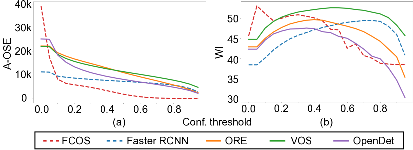
Figure 3: A-OSE (a) and WI (b) of different methods at different detector operating points. Smaller values mean better performance for both metrics. The horizontal axis indicates the confidence threshold for selecting bounding box candidates. Methods’ ranking varies on the choice of the threshold.

In summary, A-OSE and WI are insufficient for evaluating OSOD-II performance since i) they merely measure OSOD-I performance, i.e., only one of the two error types, and ii) they are metrics at a single operating point. To precisely measure OSOD-II performance, we must use average precision (AP), the standard metric for object detection, also to evaluate unknown object detection. It should be noted that while all the previous studies of OSOD-II report APs for known object detection, only a few report APs for unknown detection, such as [16, 38], probably because of the mentioned difficulty of specifying what unknown objects to detect and what not.

3 A More Practical Scenario

This section introduces another application scenario of OSOD. Although it has been overlooked in previous studies, we frequently encounter the scenario in practice. It is free from the fundamental issue of OSOD-II, enabling practical evaluation of methods’ performance and probably making the problem easier to solve.

3.1 OSOD-III: Open at Class Level and Closed at Super-class level

Consider building a smartphone app that detects and classifies animal species. It is unrealistic to deal with all animal species at its initial deployment since there are too many classes. Thus, consider a strategy to start the app’s service with a limited number of animal species; after its deployment, we want to add new classes by detecting unseen animal classes. To do this, we must design the detector to detect unseen animals accurately while correctly detecting known animals. After detecting unseen animals, we may collect their training data and retrain the detector using them. There will be many similar cases in real-world applications.

This problem is similar to OSOD-II; we want to detect unknown, novel animals. However, unlike OSOD-II, it is unnecessary to consider arbitrary objects as detection targets. In brief, we consider only animal classes; our detector does not need to detect any non-animal object, even if it has been unseen. In other words, we consider the set of object classes closed at the super-class level (i.e., animals) and open at the individual class level under the super-class.

We call this problem OSOD-III. The differences between OSOD-I, -II, and -III are shown in Fig. 1 and Table 1. The problem is formally stated as follows:

OSOD-III   Assume we are given a closed set of object classes belonging to a single super-class. Then, we want to detect and classify objects of these known classes correctly and to detect every unknown class object belonging to the same super-class and classify it as “unknown.”

It is noted that there may be multiple super-classes instead of a single. In that case, we need only consider the union of the super-classes. For the sake of simplicity, we only consider the case of a single super-class in what follows.

3.2 Advantages of OSOD-III

While the applicability of OSOD-III is narrower than OSOD-II by definition, OSOD-III has two good properties.

One is that OSOD-III is free from the fundamental difficulty of OSOD-II, the dilemma of determining what unknown objects to detect and what to not. Indeed, the judgment is clear with OSOD-III; unknowns belonging to the known super-class should be detected, and all other unknowns should not. As a result, OSOD-III no longer suffers from the evaluation difficulty. The clear identification of detection targets enables the computation of AP also for unknown objects.

The other is that detecting unknowns will arguably be easier owing to the similarity between known and unknown classes. In OSOD-II, unknown objects can be arbitrarily dissimilar from known objects. In OSOD-III, known and unknown objects share their super-class, leading to their visual similarity. It should be noted here that what we regard as a super-class is arbitrary; there is no mathematical definition. However, as far as we consider reasonable class hierarchy as in WordNet/ImageNet [10, 5] , we may say that the sub-classes will share visual similarities.

4 Experimental Results

Based on the above formalization, we evaluate the performance of existing OSOD methods on the proposed OSOD-III scenario. In the following section, we first introduce our experimental settings to simulate the OSOD-III scenario and then report the evaluation results.

4.1 Experimental Settings

4.1.1 Datasets

We use the following three datasets for the experiments: Open Images Dataset v6 [20], Caltech-UCSD Birds-200-2011 (CUB200) [37], and Mapillary Traffic Sign Dataset (MTSD) [8]. For each, we split classes into known/unknown and images into training/validation/testing subsets as explained below. Note that two of the compared methods, ORE [18] and VOS [7], need validation images (i.e., example unknown-class instances), which may be regarded as leakage in OSOD problems. This does not apply to the other methods.

Open Images   Open Images [20] contains 1.9M images of 601 classes of diverse objects with 15.9M bounding box annotations. It also provides the hierarchy of object classes in a tree structure, where each node represents a super-class, and each leaf represents an individual object category. For instance, a leaf Polar Bear has a parent node Carnivore. We choose two super-classes, Animal and Vehicle, in our experiments because of their appropriate numbers of sub-classes, i.e., 96 and 24 in the “Animal” and “Vehicle” super-class, respectively. We split these sub-classes into known and unknown classes. To mitigate statistical biases, we consider four random splits and select one for a known-class set and the union of the other three for an unknown-class set. We report the result for each of the four splits and their average.

We construct the training/validation/testing splits of images based on the original splits provided by the dataset. Specifically, we choose the images containing at least one known-class instance from the original training and validation splits. We choose the images containing either at least one known-class instance or at least one unknown-class instance from the original testing split. For the training images, we keep annotations for the known objects and eliminate all other annotations including unknown objects. It should be noted that there is a risk that those removed objects could be treated as the “background” class. For the validation and testing images, we keep the annotations for known and unknown objects and remove all other irrelevant objects. See the supplementary material for more details.

CUB200   Caltech-UCSD Birds-200-2011 (CUB200) [37] is a 200 fine-grained bird species dataset. It contains 12k images, for each of which a single box is provided. We split the 200 classes randomly into four splits, each with 50 classes. We then choose three to form a known-class set and treat the rest as an unknown-class set. We report the results for the four known/unknown splits and their average. We construct the training/validation/testing splits similarly to Open Images with two notable exceptions. One is that we create the training/validation/test splits from the dataset’s original training/validation splits. This is because the dataset does not provide annotation for the original test split. The other is that we remove all the images containing unknown objects from the training splits. This will make the setting more rigorous.See the supplementary material for more details.

MTSD   Mapillary Traffic Sign Dataset (MTSD) [8] is a dataset of 400 diverse traffic signs from different regions around the world. It contains 52k street-level images with 260k manually annotated traffic sign instances. For the split of known/unknown classes, we consider a practical use case of OSOD-III, where a detector trained using the data from a specific region is used in another region, which might have unknown traffic signs. As the dataset does not provide region information for each image, we divide the 400 traffic sign classes into clusters based on their co-occurrence in the same images. Specifically, we apply normalized graph cut [30] to obtain three clusters, ensuring any pairs of the clusters share the minimum co-occurrence. We then use the largest cluster as a known-class set (230 classes). Denoting the other two clusters by unknown1 (55) and unknown2 (115), we test three cases, i.e., using either unknown1, unknown2, or their union (unknown1+2) for a unknown-class set. We report the results for the three cases. We create the training/validation/testing splits in the same way as CUB200. See the supplementary material for more details.

4.1.2 Evaluation

Table 3: Detection accuracy of known (AP_known) and unknown objects (AP_unk) of different methods for Open Images dataset, “Animal” and “Vehicle” super-classes. “Split-$n$” indicates that the classes of Split-$n$ are treated as known classes. “mean” is their average.

	Animal
	Split1		Split2		Split3		Split4		mean
	${\rm AP}_{known}$	${\rm AP}_{unk}$	${\rm AP}_{known}$	${\rm AP}_{unk}$	${\rm AP}_{known}$	${\rm AP}_{unk}$	${\rm AP}_{known}$	${\rm AP}_{unk}$	${\rm AP}_{known}$	${\rm AP}_{unk}$
ORE [18]	$40.4$	$17.4$	$34.8$	$13.0$	$40.4$	$19.1$	$34.8$	$13.0$	$37.6\pm 2.8$	$15.6\pm 2.7$
VOS [7]	$39.4$	$10.2$	$37.4$	$4.9$	$42.9$	$5.1$	$37.8$	$4.3$	$39.4\pm 2.2$	$6.1\pm 2.4$
OpenDet [16]	$42.4$	$34.9$	$23.2$	$25.8$	$43.0$	$37.9$	$39.0$	$33.5$	$36.9\pm 8.1$	$33.0\pm 4.5$
FCOS [34]	$35.0$	$44.4$	$30.8$	$35.6$	$32.6$	$43.7$	$22.6$	$43.6$	$30.3\pm 4.7$	$41.8\pm 3.6$
Faster RCNN [28]	$42.2$	$35.1$	$33.3$	$28.6$	$36.5$	$36.6$	$35.0$	$36.3$	$36.8\pm 3.3$	$34.2\pm 3.3$
	Vehicle
	Split1		Split2		Split3		Split4		mean
	${\rm AP}_{known}$	${\rm AP}_{unk}$	${\rm AP}_{known}$	${\rm AP}_{unk}$	${\rm AP}_{known}$	${\rm AP}_{unk}$	${\rm AP}_{known}$	${\rm AP}_{unk}$	${\rm AP}_{known}$	${\rm AP}_{unk}$
ORE [18]	$46.9$	$0.5$	$35.0$	$0.1$	$25.0$	$0.2$	$27.7$	$0.3$	$33.7\pm 8.5$	$0.3\pm 0.1$
VOS [7]	$46.6$	$5.3$	$40.9$	$5.9$	$32.1$	$7.7$	$34.0$	$8.7$	$38.4\pm 5.8$	$6.9\pm 1.4$
OpenDet [16]	$50.6$	$10.2$	$40.4$	$12.5$	$30.2$	$15.9$	$33.6$	$19.0$	$38.7\pm 7.8$	$14.4\pm 3.3$
FCOS [34]	$49.6$	$14.2$	$32.7$	$14.6$	$19.2$	$24.7$	$21.4$	$21.3$	$30.7\pm 12.0$	$18.7\pm 4.5$
Faster RCNN [28]	$50.4$	$10.8$	$40.7$	$15.7$	$32.4$	$18.9$	$35.6$	$18.0$	$39.8\pm 6.8$	$15.9\pm 3.1$

Table 4: Detection accuracy for CUB200 [37]. See Table 3 for notations.

	Split1		Split2		Split3		Split4		mean
	${\rm AP}_{known}$	${\rm AP}_{unk}$	${\rm AP}_{known}$	${\rm AP}_{unk}$	${\rm AP}_{known}$	${\rm AP}_{unk}$	${\rm AP}_{known}$	${\rm AP}_{unk}$	${\rm AP}_{known}$	${\rm AP}_{unk}$
ORE [18]	$51.3$	$18.1$	$53.6$	$21.8$	$54.4$	$17.7$	$53.6$	$21.6$	$53.2\pm 1.3$	$19.8\pm 2.2$
VOS [7]	$58.1$	$5.1$	$57.6$	$6.2$	$58.9$	$4.3$	$55.4$	$6.8$	$57.5\pm 1.5$	$5.6\pm 1.1$
OpenDet [16]	$63.9$	$23.1$	$63.6$	$30.0$	$63.9$	$26.3$	$61.6$	$28.6$	$63.3\pm 1.1$	$27.0\pm 3.0$
FCOS [34]	$55.0$	$23.0$	$55.2$	$26.1$	$50.6$	$25.0$	$53.0$	$24.6$	$53.5\pm 2.1$	$24.7\pm 1.3$
Faster RCNN [28]	$57.0$	$18.9$	$58.0$	$22.5$	$59.6$	$21.1$	$57.3$	$20.5$	$58.0\pm 1.2$	$20.8\pm 1.5$

Table 5: Detection accuracy for MTSD [8]. K, U1, and U2 stand for known, unknown1, and unknown2, respectively.

	K	U1	U2	U1+2	mean
	${\rm AP}_{known}$	${\rm AP}_{unk}$
ORE [18]	$41.2$	$0.4$	$0.2$	$0.7$	$0.4\pm 0.3$
VOS [7]	$48.0$	$2.9$	$1.2$	$3.2$	$2.4\pm 1.1$
OpenDet [16]	$51.8$	$8.7$	$6.7$	$14.2$	$9.9\pm 3.9$
FCOS [34]	$41.7$	$3.8$	$3.3$	$6.2$	$4.4\pm 1.6$
Faster RCNN [28]	$48.2$	$2.5$	$2.3$	$4.1$	$3.0\pm 1.0$

As discussed earlier, the primary metric for evaluating object detection performance is average precision (AP) [11, 9]. Although we must use AP for unknown detection, the issue with OSOD-II makes it impractical. OSOD-III is free from the issue, and we can use AP for unknown object detection. Therefore, following the standard evaluation procedure of object detection, we report AP over IoU in the range $[0.50,0.95]$ for known and unknown object detection.

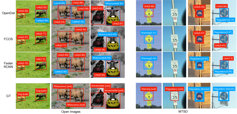
Figure 4: Example outputs of OpenDet [16] and our two baseline methods for Open Images with Animal and Vehicle super-classes (left) and MTSD (right), respectively. Red and blue boxes indicate detected unknown-class and known-class objects, respectively; “Unk” means “unknown”. The numbers in the parentheses are detection scores. We show only boxes with confidence threshold $\geq 0.3$.

4.2 Compared Methods

We consider three state-of-the-art OSOD methods [18, 7, 16]. While they are originally developed to deal with OSOD-II, these methods can be applied to OSOD-III without little or no modification. We first summarize these methods and their configurations in our experiments below, followed by the introduction of a simple baseline method that detects unknown objects merely from the outputs of a standard detector.

ORE (Open World Object Detector) [18] is initially designed for OWOD; it is capable not only of detecting unknown objects but also of incremental learning. We omit the latter capability and use the former as an open-set object detector. It employs an energy-based method to classify known/unknown; using the validation set, including unknown object annotations, it models the energy distributions for known and unknown objects. To compute AP for unknown objects, we need a score for their detection. ORE provides one, and we use it for the AP computation. Following the paper [18], we employ Faster RCNN [28] with a ResNet50 backbone [17] for the base detector.

VOS (Virtual Outlier Synthesis) [7] detects unknown objects by treating them as out-of-distribution (OOD) based on an energy-based method. Specifically, it estimates an energy value for each detected instance and judges whether it is known or unknown by comparing the energy with a threshold. Following the original study [7], we choose the threshold using the validation set so that 95% of known object instances are correctly classified. Unlike other OSOD methods, VOS does not provide a detection score for unknown objects. To compute AP, we use the energy value for the purpose. We use Faster RCNN with ResNet50-FPN backbone [22], following the paper.

OpenDet (Open-set Detector) [16] is the current state-of-the-art on the popular benchmark test designed using PASCAL VOC/COCO shown in Table 2, although the methods’ performance is evaluated with inappropriate metrics of A-OSE and WI. OpenDet provides a detection score for unknown objects, which we utilize to compute AP. We use the authors’ implementation, which employs Faster RCNN based on ResNet50-FPN for the base detector.

Simple Baselines   We consider a naive baseline for comparison. It merely uses the class scores that standard detectors predict for each bounding box. It relies on an expectation that unknown-class inputs should result in uncertain class prediction. Thus we look at the prediction uncertainty to judge if the input belongs to known/unknown classes. Specifically, we calculate the ratio of the top-1 and top-2 class scores for each candidate bounding box and compare it with a pre-defined threshold $\gamma$; we regard the input as unknown if it is smaller than $\gamma$ and as known otherwise. We use the sum of the top three class scores for the unknown object detection score. In our experiments, we employ two detectors, FCOS [34] and Faster RCNN [28]. We use ResNet50-FPN as their backbone, following the above methods. For Open Images, we set $\gamma=4.0$ for FCOS and $\gamma=15.0$ for Faster RCNN. For CUB200 and MTSD, we set $\gamma=1.5$ for FCOS and $\gamma=3.0$ for Faster RCNN. We need different thresholds due to the difference in the number of classes and the output layer design, i.e., logistic vs. softmax. We report the sensitivity to the choice of $\gamma$ in the supplementary.

4.3 Results

Table 3 shows the results of Open Images with two settings of choosing “Animal” and “Vehicle” as super-classes. It shows mAP for the known-class objects, denoted by ${\rm AP}_{known}$, and AP for the unknown objects, denoted by ${\rm AP}_{unk}$, for each of the four known/unknown class splits, and their averages with standard deviations.

We can see from the table that the compared methods attain similar ${\rm AP}_{known}$ (except the FCOS-based baseline due to the difference in the base detector). However, they show diverse performances in unknown object detection measured by ${\rm AP}_{unk}$. Specifically, ORE and VOS yield inferior performance. While the rest of the methods achieve much better performance, we can observe that the two baseline methods outperform OpenDet, the current state-of-the-art. This good performance of these baseline methods is remarkable, considering that they do not require additional training or mechanism dedicated to unknown detection.

Table 4 shows the results for CUB200. We have similar observations with a few minor differences. Differences are that ORE works better for this dataset and OpenDet achieves the best performance. However, the gap between OpenDet and the baseline methods is not large with $\mathrm{AP}_{known}$ and $\mathrm{AP}_{unk}$.

Table 5 shows the results for MTSD. We have the following observations. First, similarly to the above datasets, all the methods maintain the good performance of known object detection; $\mathrm{AP}_{known}$’s are high. Second, OpenDet performs the best unknown detection performance with noticeable margins to others for this dataset. However, its accuracy is very low, i.e., $9.9\pm 3.9$. In other words, even the best performer, OpenDet, achieves only very limited unknown detection performance. This level of performance will be insufficient for real-world applications; we need a more effective method.

Figure 4 shows selected examples of detection results by OpenDet and the two baselines for Open Images (left) and MTSD (right). We can see that the three methods behave mostly similarly. For both datasets, there are erroneous detection results of treating unknown as known and vice versa, in addition to simple false negatives of unknown detection. For Open Images, the three methods successfully detect some, not all, unknown animals/vehicles, such as “Dog” and “Snowmobile.” All the methods do not perform well for MTSD. These are consistent with the quantitative results in Tables 3 and 5. Additionally, the detectors often output two boxes for the same object instances with known and unknown labels. We may need additional non-maximum suppression to select one of these, which may potentially be a critical issue specific to OSOD that is underexplored. See the supplementary material for more visualization results.

5 Related Work

5.1 Open-Set Recognition

For the safe deployment of neural networks, open-set recognition (OSR) has attracted considerable attention. The task of OSR is to accurately classify known objects and simultaneously detect unseen objects as unknown. Scheirer et al. [29] first formalized the problem of OSR, and many following studies have been conducted so far [2, 13, 26, 33, 27, 31, 35, 43].

The work of Bendale and Boult [2] is the first to apply deep neural networks to OSR. They use outputs from the penultimate layer of a network to calibrate its prediction scores. Several studies found generative models are effective for OSR, where unseen-class images are synthesized and used for training. Generative Openmax [13] and a counterfactual method [26] use a generative adversarial network [14] to synthesize unseen-class images that are dissimilar to seen-class images. OpenGAN [19] improves the performance of OSR by generating unseen-class samples in the latent space. Another line of OSR studies focuses on a reconstruction-based method using latent features [40, 39], class conditional auto-encoder [27], and conditional gaussian distributions [33]. Zhou et al. [43] employ two types of placeholders to improve OSR; classifier placeholders to distinguish unknown objects from known classes and data placeholders to synthesize novel instances using manifold mixup [36].

5.2 Open-Set Object Detection

Recently, increasing attention has been paid to open-set object detection (OSOD). We can categorize OSOD problems into two scenarios, OSOD-I and -II, according to their different interest in unknown objects, as we have discussed in this paper.

OSOD-I  Early studies treat OSOD as an extension of OSR problem [25, 24, 6]. They aim to correctly detect every known object instance and avoid misclassifying any unseen object instance into known classes. Miller et al. [25] first utilize multiple inference results through dropout layers [12] to estimate the uncertainty of the detector’s prediction and use it to avoid erroneous detections under open-set conditions. A follow-up work finds that the proper choice of merging strategy applied to the multiple inferences leads to better detection performance. Dhamija et al. [6] investigate how modern CNN detectors behave in an open-set environment and reveal that the detectors detect unseen objects as known objects with a high confidence score. For the evaluation, researchers have employed A-OSE [25] and WI [6] as the primary metrics to measure the accuracy of detecting known objects. They are designed to measure how frequently a detector wrongly detects and classifies unknown objects as known objects.

OSOD-II  More recent studies have moved in a more in-depth direction, where they aim to correctly detect/classify every object instance not only with the known class but also with the unknown class. This scenario is often considered a part of open-world object detection (OWOD) [18, 15, 41, 32, 38]. In this case, the detection of unknown objects matters since it considers updating the detectors by collecting unknown classes and using them for retraining. Joseph et al. [18] first introduces the concept of OWOD and establishes the benchmark test. Many subsequent works have strictly followed this benchmark and proposed methods for OSOD. OW-DETR [15] introduces a transformer-based detector (i.e., DETR [3, 44]) for OWOD and improves the performance. Han et al. [16] propose OpenDet and pay attention to the fact that unknown classes are distributed in low-density regions in the latent space. They then perform contrastive learning to encourage intra-class compactness and inter-class separation of known classes, leading to performance gain. Similarly, Du et al. [7] synthesize virtual unseen samples from the decision boundaries of gaussian distributions for each known class. Wu et al. [38] propose a further challenging task to distinguish unknown instances as multiple unknown classes.

6 Conclusion

In this paper, we have considered the problem of open-set object detection (OSOD). Classifying the formalization of OSOD in previous studies into two, i.e., OSOD-I and -II, we first pointed out the ill-posedness of OSOD-II. Specifically, it is difficult to determine what to detect and what not for unknown objects. This difficulty makes the evaluation infeasible; as a result, the previous studies employ insufficient metrics, A-OSE and WI, for methods’ evaluation. They are originally designed for OSOD-I and do not measure the accuracy of unknown object detection.

We then introduced a new scenario, OSOD-III. It considers the detection of unknown objects belonging to the same super-class as the known objects. This formalization resolves the above issues of OSOD-II. We can determine what to detect or not in advance and then appropriately evaluate methods’ performance using a standard AP metric for known and unknown detection. We also design benchmark tests tailored to the proposed scenario and evaluate the existing OSOD methods and a baseline method we designed in this paper on them. The results have shown that the state-of-the-art methods attain only limited performance, similar to the baseline. We concluded that we need a better OSOD method. Additionally, our categorization of OSOD problems provides a new taxonomy. We hope our study helps the community rethink the OSOD problems and progress in the right direction.

Appendix A More Details of Experimental Settings

A.1 Dataset Details

We used three datasets in our experiments, i.e., Open Images [20], Caltech-UCSD Birds-200-2011 (CUB200) [37], and Mapillary Traffic Sign Dataset (MTSD) [8]. Tables 6, 7, and 8 show their splits, based on which known/unknown classes are selected, and also those of training/validation/testing images. Tables 9, 10, and 11provide lists of the classes for each split. Please check Sec 4.1.1 in the main paper as well.

Table 6: Details of the employed class splits for Open Images dataset. We treat one of the four as a known set and the union of the other three as an unknown set. Thus, there are four cases of known/unknown splits, for each of which we report the detection performance in Table 3 of the main paper.

	Animal				Vehicle
	Split1	Split2	Split3	Split4	Split1	Split2	Split3	Split4
num of known categories	$24$	$24$	$24$	$24$	$6$	$6$	$6$	$6$
train images	$44,379$	$38,914$	$39,039$	$18,478$	$43,270$	$26,860$	$3,900$	$6,300$
validation images	$1,104$	$2,353$	$1,248$	$849$	$1,370$	$503$	$178$	$322$
test images	$15,609$				$6,991$

Table 7: Details of the employed class splits for Caltech-UCSD Birds-200-2011 (CUB200) dataset. We treat the union of three of the four as known classes and the rest as unknown classes. Each split corresponds to the results shown in Table 4.

	Split1	Split2	Split3	Split4
num of unknown classes	$50$	$50$	$50$	$50$
train images	$4,109$	$4,116$	$4,120$	$4,120$
validation images	$500$	$500$	$500$	$500$
test images	$5,794$

Table 8: Details of the employed class splits for Mapillary Traffic Sign Dataset (MTSD). Each split corresponds to the results shown in Table 5.

	Unknown1	Unknown2	Unknown1+2
num of classes	$55$	$115$	$170$
train images	$13,157$
validation images	$1,000$	$1,000$	$1,000$
test images	$3,896$

Table 9: Classes contained in the employed splits for Open Images [20] with the super-classes “Animal” (upper row) and “Vehicle” (bottom row), respectively.

	Split1	Split2	Split3	Split4
Animal (96)	Starfish / Deer / Tick / Lynx / Monkey / Squirrel / Koala / Fox / Spider / Scorpion / Rabbit / Hamster / Woodpecker / Snail / Brown bear / Polar bear / Lion / Bull / Shrimp / Panda / Chicken / Sparrow / Cattle / Lobster	Sea lion / Mule / Lizard / Raccoon / Butterfly / Hippopotamus / Kangaroo / Frog / Harbor seal / Red panda / Antelope / Ant / Sheep / Dog / Magpie / Teddy bear / Oyster / Otter / Seahorse / Caterpillar / Worm / Zebra / Jaguar (Animal) / Rays and skates	Tortoise / Skunk / Blue jay / Rhinoceros / Turkey / Falcon / Dinosaur / Bat (Animal) / Squid / Giraffe / Owl / Armadillo / Swan / Duck / Goose / Camel / Horse / Tiger / Goldfish / Cat / Shark / Parrot / Leopard / Goat	Dragonfly / Ladybug / Raven / Penguin / Hedgehog / Mouse / Snake / Jellyfish / Porcupine / Ostrich / Elephant / Dolphin / Alpaca / Crab / Eagle / Isopod / Cheetah / Sea turtle / Whale / Bee / Canary / Pig / Crocodile / Centipede
Vehicle (24)	Bicycle / Golf cart / Van / Taxi / Airplane / Motorcycle	Train / Truck / Barge / Gondola / Rocket / Bus	Submarine / Jet ski / Unicycle / Snowmobile / Cart / Tank	Canoe / Helicopter / Wheelchair / Ambulance / Segway / Limousine

Table 10: Classes contained in the employed splits for CUB200 [37].

Split1	Split2	Split3	Split4
Black footed Albatross / Laysan Albatross / Least Auklet / Red winged Blackbird / Yellow headed Blackbird / Indigo Bunting / Spotted Catbird / Brandt Cormorant / Red faced Cormorant / Shiny Cowbird / Brown Creeper / Yellow billed Cuckoo / Purple Finch / Acadian Flycatcher / Scissor tailed Flycatcher / Vermilion Flycatcher / Western Grebe / Ivory Gull / Ruby throated Hummingbird / Rufous Hummingbird / Green Jay / Belted Kingfisher / Pied Kingfisher / Pacific Loon / Mallard / Western Meadowlark / Orchard Oriole / Scott Oriole / Whip poor Will / Loggerhead Shrike / Great Grey Shrike / Brewer Sparrow / Grasshopper Sparrow / Henslow Sparrow / Le Conte Sparrow / Cape Glossy Starling / Bank Swallow / Tree Swallow / Common Tern / Least Tern / Philadelphia Vireo / Wilson Warbler / Pileated Woodpecker / Red bellied Woodpecker / Red cockaded Woodpecker / Bewick Wren / Marsh Wren / Rock Wren / Winter Wren / Common Yellowthroat	Groove billed Ani / Crested Auklet / Parakeet Auklet / Bobolink / Lazuli Bunting / Gray Catbird / Fish Crow / Gray crowned Rosy Finch / Least Flycatcher / Gadwall / Blue Grosbeak / Heermann Gull / Ring billed Gull / Slaty backed Gull / Green Violetear / Pomarine Jaeger / Red breasted Merganser / Mockingbird / White breasted Nuthatch / Baltimore Oriole / Western Wood Pewee / American Pipit / Geococcyx / Baird Sparrow / House Sparrow / Field Sparrow / Seaside Sparrow / Vesper Sparrow / White throated Sparrow / Cliff Swallow / Scarlet Tanager / Summer Tanager / Elegant Tern / Forsters Tern / Green tailed Towhee / Brown Thrasher / Blue headed Vireo / White eyed Vireo / Bay breasted Warbler / Black and white Warbler / Golden winged Warbler / Nashville Warbler / Orange crowned Warbler / Palm Warbler / Pine Warbler / Swainson Warbler / Tennessee Warbler / Bohemian Waxwing / American Three toed Woodpecker / Carolina Wren	Sooty Albatross / Rhinoceros Auklet / Brewer Blackbird / Rusty Blackbird / Painted Bunting / Cardinal / Chuck will Widow / Pelagic Cormorant / Bronzed Cowbird / American Crow / Mangrove Cuckoo / Yellow bellied Flycatcher / Northern Fulmar / European Goldfinch / Boat tailed Grackle / Horned Grebe / Evening Grosbeak / Pigeon Guillemot / Herring Gull / Western Gull / Anna Hummingbird / Long tailed Jaeger / Gray Kingbird / Green Kingfisher / Horned Lark / Clark Nutcracker / Brown Pelican / Sayornis / Common Raven / White necked Raven / Black throated Sparrow / Chipping Sparrow / Clay colored Sparrow / Fox Sparrow / Savannah Sparrow / White crowned Sparrow / Barn Swallow / Black Tern / Caspian Tern / Sage Thrasher / Red eyed Vireo / Cape May Warbler / Chestnut sided Warbler / Kentucky Warbler / Mourning Warbler / Prairie Warbler / Yellow Warbler / Louisiana Waterthrush / Red headed Woodpecker / Cactus Wren	Yellow breasted Chat / Eastern Towhee / Black billed Cuckoo / Northern Flicker / Great Crested Flycatcher / Olive sided Flycatcher / Frigatebird / American Goldfinch / Eared Grebe / Pied billed Grebe / Pine Grosbeak / Rose breasted Grosbeak / California Gull / Glaucous winged Gull / Blue Jay / Florida Jay / Dark eyed Junco / Tropical Kingbird / Ringed Kingfisher / White breasted Kingfisher / Red legged Kittiwake / Hooded Merganser / Nighthawk / Hooded Oriole / Ovenbird / White Pelican / Horned Puffin / American Redstart / Harris Sparrow / Lincoln Sparrow / Nelson Sharp tailed Sparrow / Song Sparrow / Tree Sparrow / Artic Tern / Black capped Vireo / Warbling Vireo / Yellow throated Vireo / Black throated Blue Warbler / Blue winged Warbler / Canada Warbler / Cerulean Warbler / Hooded Warbler / Magnolia Warbler / Myrtle Warbler / Prothonotary Warbler / Worm eating Warbler / Northern Waterthrush / Cedar Waxwing / Downy Woodpecker / House Wren

Table 11: Classes contained in the Unknown1 and Unkonwn2 splits of MTSD [8]. The rest are treated as known classes.

Unknown1

Unknown2

complementary–chevron-left–g1 / complementary–chevron-right–g1 / complementary–maximum-speed-limit-20–g1 / complementary–maximum-speed-limit-25–g1 / complementary–maximum-speed-limit-30–g1 / complementary–maximum-speed-limit-35–g1 / complementary–maximum-speed-limit-40–g1 / complementary–maximum-speed-limit-45–g1 / complementary–maximum-speed-limit-50–g1 / complementary–maximum-speed-limit-55–g1 / complementary–maximum-speed-limit-70–g1 / complementary–maximum-speed-limit-75–g1 / information–highway-exit–g1 / information–safety-area–g2 / regulatory–detour-left–g1 / regulatory–keep-right–g6 / regulatory–no-overtaking–g5 / regulatory–weight-limit-with-trucks–g1 / warning–accidental-area-unsure–g2 / warning–bus-stop-ahead–g3 / warning–curve-left–g2 / warning–curve-right–g2 / warning–domestic-animals–g3 / warning–double-curve-first-left–g2 / warning–double-curve-first-right–g2 / warning–double-turn-first-right–g1 / warning–falling-rocks-or-debris-right–g2 / warning–falling-rocks-or-debris-right–g4 / warning–hairpin-curve-left–g1 / warning–hairpin-curve-right–g1 / warning–hairpin-curve-right–g4 / warning–horizontal-alignment-left–g1 / warning–horizontal-alignment-right–g1 / warning–horizontal-alignment-right–g3 / warning–junction-with-a-side-road-acute-right–g1 / warning–junction-with-a-side-road-perpendicular-left–g3 / warning–junction-with-a-side-road-perpendicular-right–g3 / warning–kangaloo-crossing–g1 / warning–loop-270-degree–g1 / warning–narrow-bridge–g1 / warning–offset-roads–g3 / warning–railroad-crossing-with-barriers–g2 / warning–railroad-intersection–g4 / warning–road-widens–g1 / warning–road-widens-right–g1 / warning–slippery-motorcycles–g1 / warning–slippery-road-surface–g2 / warning–steep-ascent–g7 / warning–trucks-crossing–g1 / warning–turn-left–g1 / warning–turn-right–g1 / warning–winding-road-first-left–g1 / warning–winding-road-first-right–g1 / warning–wombat-crossing–g1 / warning–y-roads–g1 /

complementary–both-directions–g1 / complementary–chevron-right–g3 / complementary–go-left–g1 / complementary–go-right–g1 / complementary–go-right–g2 / complementary–keep-left–g1 / complementary–keep-right–g1 / complementary–maximum-speed-limit-15–g1 / complementary–one-direction-left–g1 / complementary–one-direction-right–g1 / complementary–turn-left–g2 / complementary–turn-right–g2 / information–airport–g2 / information–bike-route–g1 / information–camp–g1 / information–gas-station–g1 / information–highway-interstate-route–g2 / information–hospital–g1 / information–interstate-route–g1 / information–lodging–g1 / information–parking–g3 / information–parking–g6 / information–trailer-camping–g1 / regulatory–bicycles-only–g2 / regulatory–bicycles-only–g3 / regulatory–do-not-block-intersection–g1 / regulatory–do-not-stop-on-tracks–g1 / regulatory–dual-lanes-go-straight-on-left–g1 / regulatory–dual-lanes-go-straight-on-right–g1 / regulatory–dual-lanes-turn-left-no-u-turn–g1 / regulatory–dual-lanes-turn-left-or-straight–g1 / regulatory–dual-lanes-turn-right-or-straight–g1 / regulatory–go-straight–g3 / regulatory–go-straight-or-turn-left–g2 / regulatory–go-straight-or-turn-left–g3 / regulatory–go-straight-or-turn-right–g3 / regulatory–keep-right–g4 / regulatory–lane-control–g1 / regulatory–left-turn-yield-on-green–g1 / regulatory–maximum-speed-limit-100–g3 / regulatory–maximum-speed-limit-25–g2 / regulatory–maximum-speed-limit-30–g3 / regulatory–maximum-speed-limit-35–g2 / regulatory–maximum-speed-limit-40–g3 / regulatory–maximum-speed-limit-40–g6 / regulatory–maximum-speed-limit-45–g3 / regulatory–maximum-speed-limit-50–g6 / regulatory–maximum-speed-limit-55–g2 / regulatory–maximum-speed-limit-65–g2 / regulatory–no-left-turn–g1 / regulatory–no-parking–g2 / regulatory–no-parking-or-no-stopping–g1 / regulatory–no-parking-or-no-stopping–g2 / regulatory–no-parking-or-no-stopping–g3 / regulatory–no-right-turn–g1 / regulatory–no-stopping–g2 / regulatory–no-stopping–g4 / regulatory–no-straight-through–g1 / regulatory–no-turn-on-red–g1 / regulatory–no-turn-on-red–g2 / regulatory–no-turn-on-red–g3 / regulatory–no-turns–g1 / regulatory–no-u-turn–g1 / regulatory–one-way-left–g2 / regulatory–one-way-left–g3 / regulatory–one-way-right–g2 / regulatory–one-way-right–g3 / regulatory–parking-restrictions–g2 / regulatory–pass-on-either-side–g2 / regulatory–passing-lane-ahead–g1 / regulatory–reversible-lanes–g2 / regulatory–road-closed–g2 / regulatory–roundabout–g2 / regulatory–stop–g1 / regulatory–stop-here-on-red-or-flashing-light–g1 / regulatory–stop-here-on-red-or-flashing-light–g2 / regulatory–text-four-lines–g1 / regulatory–triple-lanes-turn-left-center-lane–g1 / regulatory–truck-speed-limit-60–g1 / regulatory–turn-left–g2 / regulatory–turn-right–g3 / regulatory–turning-vehicles-yield-to-pedestrians–g1 / regulatory–wrong-way–g1 / warning–added-lane-right–g1 / warning–bicycles-crossing–g2 / warning–bicycles-crossing–g3 / warning–divided-highway-ends–g2 / warning–double-reverse-curve-right–g1 / warning–dual-lanes-right-turn-or-go-straight–g1 / warning–emergency-vehicles–g1 / warning–equestrians-crossing–g2 / warning–flaggers-in-road–g1 / warning–height-restriction–g2 / warning–junction-with-a-side-road-perpendicular-left–g4 / warning–pass-left-or-right–g2 / warning–pedestrians-crossing–g4 / warning–pedestrians-crossing–g9 / warning–playground–g1 / warning–playground–g3 / warning–railroad-crossing–g1 / warning–railroad-intersection–g3 / warning–road-narrows-left–g2 / warning–road-narrows-right–g2 / warning–roundabout–g25 / warning–school-zone–g2 / warning–shared-lane-motorcycles-bicycles–g1 / warning–stop-ahead–g9 / warning–texts–g1 / warning–texts–g2 / warning–texts–g3 / warning–traffic-merges-right–g1 / warning–traffic-signals–g3 / warning–trail-crossing–g2 / warning–two-way-traffic–g2 /

A.2 Training

We train the models using the SGD optimizer with the batch size of $16$. We train each model with $12$ epochs for Open Images; $80$ epochs for CUB200 dataset; $60$ epochs for MTSD for each. We use the initial learning rate of $2.0\times 10^{-2}$ with momentum $=0.9$ and weight decay $=1.0\times 10^{-4}$. We drop a learning rate by a factor of 10 at $2/3$ and $11/12$ epoch.

We used the publicly available source code for the implementation of ORE [18], VOS [7], and OpenDet [16]. We used mmdetection [4] to implement FCOS [34] and Faster RCNN [28] for the baseline methods.

Appendix B Results of A-OSE and WI

In this study, we use the average precision for unknown object detection, denoted by ${\rm AP}_{unk}$, as a primary metric to evaluate OSOD methods, as reported in Table 3, 4, and 5. For the readers’ information, we report here absolute open-set error (A-OSE) and wilderness impact (WI), the metrics widely used in previous studies. Tables 12, 13, and 14 show those for the compared methods on the same test data. Recall that i) A-OSE and WI measure only detectors’ performance of known object detection; and ii) they evaluate detectors’ performance at a single operating point. Tables 12, 13, and 14 show the results at the operating points chosen in the previous studies, i.e., confidence score $>0.05$ for A-OSE and the recall (of known object detection) $=0.8$ for WI, respectively.

The results show that OpenDet and Faster RCNN achieve comparable performance on both metrics. FCOS performs worse, but this is not necessarily true at different operating points, as shown in Fig. 3 of the main paper. We can also see from the results a clear inconsistency between the A-OSE/WI and ${\rm AP}$s. For instance, as shown in Table 13, Faster RCNN is inferior to VOS in both the A-OSE and WI metrics (i.e., $5,567\pm 203$ vs. $4,415\pm 498$ on A-OSE), whereas it achieves much better ${\rm AP}_{known}$ and ${\rm AP}_{unk}$ than VOS, as shown in Table 4. Such inconsistency demonstrates that A-OSE and WI are unsuitable performance measures for OSOD-II/III.

Table 12: A-OSE and WI of the compared methods in the experiment of Open Images. The same experimental setting as Table 3 is used.

	Animal
	Split1		Split2		Split3		Split4		mean
	A-OSE	WI	A-OSE	WI	A-OSE	WI	A-OSE	WI	A-OSE	WI
ORE[18]	$23,334$	$35.9$	$17,835$	$30.8$	$22,219$	$45.3$	$25,682$	$47.0$	$22,268\pm 2,848$	$39.7\pm 6.7$
VOS [7]	$12,124$	$34.8$	$21,622$	$36.6$	$30,988$	$50.9$	$23,360$	$62.1$	$22,024\pm 6,714$	$46.1\pm 11.2$
OpenDet[16]	$26,426$	$34.9$	$22,736$	$27.7$	$25,075$	$45.6$	$26,770$	$56.1$	$25,252\pm 1,585$	$41.1\pm 10.7$
FCOS [34]	$38,858$	$35.5$	$34,677$	$37.6$	$52,234$	$59.4$	$30,895$	$49.5$	$39,166\pm 8,053$	$45.5\pm 9.6$
Faster RCNN [28]	$11,012$	$29.5$	$8,719$	$25.0$	$12,201$	$43.2$	$13,078$	$52.8$	$11,252\pm 1,636$	$37.6\pm 11.0$
	Vehicle
	Split1		Split2		Split3		Split4		mean
	A-OSE	WI	A-OSE	WI	A-OSE	WI	A-OSE	WI	A-OSE	WI
ORE [18]	$3,143$	$17.6$	$3,775$	$21.5$	$4,483$	$33.7$	$6,654$	$26.5$	$4,514\pm 1,323$	$24.9\pm 6.0$
VOS [7]	$1,460$	$12.0$	$1,985$	$23.9$	$1,796$	$38.3$	$3,090$	$20.9$	$2,083\pm 611$	$23.8\pm 9.5$
OpenDet [16]	$3,857$	$19.8$	$5,640$	$25.5$	$10,131$	$52.1$	$8,893$	$30.4$	$7,130\pm 2,502$	$31.9\pm 12.2$
FCOS [34]	$7,700$	$26.4$	$10,888$	$33.7$	$15,395$	$55.7$	$22,502$	$34.8$	$14,121\pm 5,558$	$37.6\pm 10.9$
Faster RCNN [28]	$3,060$	$19.2$	$3,585$	$23.8$	$5,083$	$52.1$	$7,013$	$29.9$	$4,685\pm 1,535$	$31.3\pm 12.6$

Table 13: A-OSE and WI of the compared methods in the experiment of CUB200. The same experimental setting as Table 4 is used.

	Split1		Split2		Split3		Split4		mean
	A-OSE	WI	A-OSE	WI	A-OSE	WI	A-OSE	WI	A-OSE	WI
ORE[18]	$5,001$	$22.6$	$4,836$	$22.4$	$4,562$	$24.1$	$4,998$	$19.3$	$4,849\pm 206$	$22.1\pm 2.0$
VOS [7]	$4,681$	$20.3$	$4,535$	$21.0$	$4,763$	$22.5$	$3,681$	$18.5$	$4,415\pm 498$	$20.6\pm 1.6$
OpenDet[16]	$4,384$	$18.6$	$4,746$	$21.1$	$4,426$	$22.6$	$4,602$	$18.0$	$4,539\pm 167$	$20.1\pm 2.2$
FCOS [34]	$15,421$	$24.1$	$18,334$	$27.8$	$21,377$	$25.8$	$16,822$	$24.6$	$17,988\pm 2,553$	$25.6\pm 1.6$
Faster RCNN [28]	$5,354$	$20.5$	$5,716$	$22.7$	$5,435$	$23.9$	$5,763$	$19.1$	$5,567\pm 203$	$21.5\pm 2.1$

Table 14: A-OSE and WI of the compared methods in the experiments of MTSD. The same setting is used as Table 5.

	Unknown1		Unknown2		Unknown1+2		mean
	A-OSE	WI	A-OSE	WI	A-OSE	WI	A-OSE	WI
ORE[18]	$1,711$	$5.5$	$2,050$	$7.0$	$3,283$	$11.7$	$2,348\pm 827$	$8.0\pm 3.3$
VOS [7]	$1,260$	$5.4$	$2,003$	$8.9$	$3,263$	$14.3$	$2,175\pm 1,013$	$9.5\pm 4.5$
OpenDet[16]	$722$	$3.8$	$1,146$	$7.8$	$1,868$	$11.6$	$1,245\pm 579$	$7.8\pm 3.9$
FCOS[34]	$4,897$	$5.7$	$7,086$	$7.1$	$11,983$	$12.8$	$7,989\pm 3,628$	$8.5\pm 3.8$
Faster RCNN[28]	$964$	$4.7$	$1,588$	$7.8$	$2,552$	$12.5$	$1,701\pm 800$	$8.4\pm 3.9$

Appendix C Effect of Hyperparameters with the Baseline Methods

Our baseline methods use the ratio of the top two class scores for the known/unknown classification, where we use the hyperparameter $\gamma$ as a threshold. Tables 15 and 16 show how the choice of $\gamma$ affects the results. We can observe that overall, while $\gamma$ (and $T$ with Faster RCNN) do affect the results, ${\rm AP}_{known}$ and ${\rm AP}_{unk}$ are not very sensitive to their choice. There is a trade-off between ${\rm AP}_{known}$ and ${\rm AP}_{unk}$, since smaller $\gamma$ tends to make the detectors overlook unknown objects while large $\gamma$’s make the detectors overlook known objects. Setting a large temperature $T(>1)$ with Faster RCNN helps improve ${\rm AP}_{unk}$, at a small sacrifice of ${\rm AP}_{known}$; too large $T$ damages performance.

The optimal choice of the hyperparameters depends on datasets and model architectures. The dependency comes from two factors. One is the difference in the output layer design, i.e., sigmoid (FCOS) vs. softmax (Faster RCNN). Faster RCNN employs a softmax layer to predict the confidence scores, while FCOS uses a sigmoid layer. Due to the winner-take-all nature of softmax, Faster RCNN needs a relatively larger $\gamma$ to convert known predictions into unknown classes. The other is the number of classes in the datasets. Our configurations with CUB200 and MTSD have $150$ and $230$ of known classes, respectively, which are larger than that of Open Images (e.g., $24$ classes for an “Animal” case). The larger the number of classes is, the more uncertain the prediction will be. Thus, small $\gamma$ is better for a small class set, and vice versa.

Table 15: Results of the FCOS baseline with different values of $\gamma$ for each dataset. The numbers represent ${\rm AP}_{known}$ / ${\rm AP}_{unk}$ / WI. OI(A) and OI(V) indicate Open Images for Animal classes and Vehicle classes, respectively.

Data \$\gamma$	1.5	2.0	3.0	4.0	5.0	10.0	15.0	50.0
OI(A)	$30.4\ /\ 30.2\ /\ 54.9$	$30.2\ /\ 34.8\ /\ 49.9$	$30.2\ /\ 39.5\ /\ 47.3$	$30.2\ /\ 41.8\ /\ 45.5$	$29.6\ /\ 43.0\ /\ 44.3$	$25.1\ /\ 44.2\ /\ 34.7$	$18.9\ /\ 43.9\ /\ 26.2$	$2.3\ /\ 40.6\ /\ 4.8$
OI(V)	$30.4\ /\ 12.9\ /\ 38.8$	$30.4\ /\ 14.8\ /\ 37.3$	$30.6\ /\ 17.2\ /\ 38.1$	$30.7\ /\ 18.7\ /\ 37.6$	$30.8\ /\ 19.7\ /\ 35.9$	$29.9\ /\ 21.9\ /\ 26.7$	$26.2\ /\ 22.0\ /\ 24.0$	$11.4\ /\ 20.2\ /\ 24.5$
CUB200	$53.4\ /\ 24.7\ /\ 25.6$	$51.5\ /\ 24.6\ /\ 23.9$	$46.9\ /\ 23.3\ /\ 19.7$	$43.1\ /\ 22.2\ /\ 16.2$	$39.8\ /\ 21.3\ /\ 13.9$	$28.2\ /\ 19.8\ /\ 8.0$	$20.2\ /\ 19.7\ /\ 6.2$	$3.3\ /\ 19.7\ /\ 2.4$
MTSD	$41.7\ /\ 4.4\ /\ 8.5$	$39.5\ /\ 5.2\ /\ 9.5$	$36.7\ /\ 6.0\ /\ 10.4$	$34.3\ /\ 6.3\ /\ 8.5$	$32.3\ /\ 6.5\ /\ 7.6$	$25.4\ /\ 6.4\ /\ 4.1$	$21.6\ /\ 6.2\ /\ 3.4$	$8.6\ /\ 5.5\ /\ 0.7$

Table 16: Results of the Faster RCNN baseline with different values of $\gamma$ and $T$ for each dataset. See Table 15 for notations.

Open Images (Animal)
$T$ \$\gamma$	1.5	2.0	3.0	4.0	5.0	10.0	15.0	50.0
0.5	$39.5\ /\ 14.7\ /\ 57.0$	$39.4\ /\ 18.1\ /\ 56.8$	$39.3\ /\ 20.8\ /\ 56.3$	$39.2\ /\ 22.3\ /\ 55.6$	$39.0\ /\ 23.4\ /\ 55.1$	$38.4\ /\ 26.0\ /\ 53.1$	$37.9\ /\ 27.3\ /\ 51.4$	$37.0\ /\ 30.6\ /\ 48.4$
0.8	$40.2\ /\ 19.4\ /\ 54.0$	$40.0\ /\ 22.5\ /\ 53.9$	$39.6\ /\ 25.4\ /\ 52.9$	$39.2\ /\ 27.1\ /\ 51.5$	$38.8\ /\ 28.2\ /\ 50.4$	$37.8\ /\ 31.1\ /\ 46.4$	$37.3\ /\ 32.4\ /\ 42.8$	$35.8\ /\ 35.0\ /\ 37.4$
1.0	$40.4\ /\ 21.6\ /\ 52.4$	$40.1\ /\ 24.6\ /\ 51.9$	$39.5\ /\ 27.5\ /\ 50.3$	$38.9\ /\ 29.1\ /\ 48.5$	$38.4\ /\ 30.3\ /\ 46.8$	$37.4\ /\ 33.0\ /\ 41.9$	$36.8\ /\ 34.2\ /\ 37.6$	$34.4\ /\ 35.8\ /\ 30.5$
2.0	$40.0\ /\ 25.4\ /\ 41.7$	$38.7\ /\ 28.0\ /\ 39.7$	$37.4\ /\ 30.7\ /\ 35.7$	$36.5\ /\ 31.9\ /\ 32.7$	$35.6\ /\ 32.5\ /\ 30.4$	$32.5\ /\ 33.1\ /\ 19.0$	$29.9\ /\ 32.8\ /\ 17.0$	$18.9\ /\ 29.8\ /\ 10.1$
3.0	$36.9\ /\ 23.2\ /\ 31.1$	$35.4\ /\ 25.6\ /\ 26.6$	$33.6\ /\ 27.5\ /\ 24.2$	$32.0\ /\ 27.9\ /\ 18.0$	$30.4\ /\ 27.9\ /\ 14.7$	$22.8\ /\ 26.5\ /\ 9.6$	$16.6\ /\ 24.7\ /\ 7.7$	$1.5\ /\ 23.2\ /\ 2.8$
5.0	$29.4\ /\ 15.4\ /\ 16.1$	$27.9\ /\ 16.9\ /\ 16.6$	$24.1\ /\ 17.5\ /\ 12.9$	$19.6\ /\ 17.1\ /\ 9.6$	$15.0\ /\ 16.5\ /\ 7.3$	$1.7\ /\ 14.9\ /\ 2.3$	$0.2\ /\ 14.8\ /\ 1.2$	$0.0\ /\ 14.8\ /\ 0.0$
Open Images (Vehicle)
$T$ \$\gamma$	1.5	2.0	3.0	4.0	5.0	10.0	15.0	50.0
0.5	$40.0\ /\ 4.1\ /\ 39.6$	$40.0\ /\ 5.4\ /\ 39.3$	$39.9\ /\ 6.7\ /\ 39.0$	$40.0\ /\ 7.4\ /\ 38.8$	$39.9\ /\ 7.8\ /\ 38.5$	$39.9\ /\ 9.3\ /\ 37.7$	$39.8\ /\ 10.1\ /\ 37.4$	$39.7\ /\ 12.0\ /\ 36.6$
0.8	$40.2\ /\ 6.6\ /\ 36.6$	$40.2\ /\ 8.1\ /\ 36.4$	$40.1\ /\ 9.6\ /\ 35.9$	$40.1\ /\ 10.5\ /\ 35.5$	$40.1\ /\ 11.2\ /\ 35.1$	$40.0\ /\ 13.0\ /\ 34.2$	$39.8\ /\ 13.9\ /\ 33.6$	$39.5\ /\ 16.3\ /\ 31.1$
1.0	$40.3\ /\ 7.9\ /\ 35.0$	$40.3\ /\ 9.6\ /\ 34.7$	$40.3\ /\ 11.2\ /\ 34.3$	$40.2\ /\ 12.2\ /\ 33.9$	$40.2\ /\ 12.8\ /\ 33.8$	$40.0\ /\ 14.8\ /\ 32.9$	$39.8\ /\ 15.8\ /\ 31.3$	$39.1\ /\ 17.9\ /\ 26.8$
2.0	$39.9\ /\ 11.7\ /\ 29.4$	$39.9\ /\ 13.5\ /\ 28.9$	$39.6\ /\ 15.5\ /\ 28.1$	$39.5\ /\ 16.8\ /\ 27.5$	$39.2\ /\ 17.6\ /\ 26.2$	$37.8\ /\ 19.2\ /\ 20.4$	$36.1\ /\ 19.6\ /\ 16.8$	$25.9\ /\ 17.4\ /\ 6.9$
3.0	$39.0\ /\ 12.7\ /\ 25.3$	$38.8\ /\ 14.7\ /\ 24.8$	$38.4\ /\ 16.9\ /\ 21.8$	$37.6\ /\ 17.9\ /\ 20.9$	$36.7\ /\ 18.4\ /\ 18.9$	$31.0\ /\ 17.9\ /\ 7.6$	$23.8\ /\ 16.3\ /\ 4.3$	$1.6\ /\ 15.3\ /\ 0.8$
5.0	$36.4\ /\ 13.3\ /\ 19.8$	$35.9\ /\ 15.6\ /\ 17.7$	$33.3\ /\ 17.0\ /\ 13.6$	$29.3\ /\ 16.6\ /\ 7.6$	$23.4\ /\ 15.2\ /\ 6.3$	$2.2\ /\ 13.9\ /\ 0.9$	$0.2\ /\ 13.9\ /\ 0.5$	$0.0\ /\ 13.9\ /\ 0.0$
CUB200
$T$ \$\gamma$	1.5	2.0	3.0	4.0	5.0	10.0	15.0	50.0
0.5	$57.9\ /\ 16.9\ /\ 22.8$	$57.9\ /\ 18.9\ /\ 22.7$	$57.7\ /\ 19.7\ /\ 22.3$	$57.6\ /\ 20.3\ /\ 22.2$	$57.5\ /\ 20.6\ /\ 21.8$	$56.4\ /\ 21.2\ /\ 21.0$	$55.0\ /\ 21.2\ /\ 19.2$	$52.4\ /\ 21.3\ /\ 16.4$
0.8	$58.5\ /\ 18.9\ /\ 22.3$	$58.4\ /\ 19.9\ /\ 22.1$	$58.1\ /\ 20.8\ /\ 21.8$	$57.6\ /\ 21.0\ /\ 21.6$	$57.1\ /\ 21.1\ /\ 21.4$	$55.0\ /\ 21.1\ /\ 18.9$	$52.9\ /\ 20.7\ /\ 16.4$	$47.7\ /\ 19.4\ /\ 11.6$
1.0	$58.7\ /\ 19.4\ /\ 21.8$	$58.6\ /\ 20.2\ /\ 21.6$	$58.0\ /\ 20.8\ /\ 21.5$	$57.2\ /\ 20.8\ /\ 21.2$	$56.4\ /\ 20.9\ /\ 20.4$	$53.2\ /\ 20.3\ /\ 17.1$	$50.6\ /\ 19.8\ /\ 14.1$	$42.9\ /\ 18.4\ /\ 8.9$
2.0	$58.0\ /\ 18.9\ /\ 19.6$	$56.9\ /\ 18.9\ /\ 19.5$	$53.9\ /\ 18.3\ /\ 17.8$	$50.9\ /\ 17.7\ /\ 15.5$	$48.4\ /\ 17.2\ /\ 13.3$	$38.3\ /\ 16.1\ /\ 7.2$	$31.3\ /\ 15.8\ /\ 5.1$	$8.9\ /\ 15.9\ /\ 2.4$
3.0	$55.5\ /\ 15.9\ /\ 17.7$	$53.0\ /\ 16.0\ /\ 16.5$	$47.3\ /\ 14.8\ /\ 12.3$	$41.6\ /\ 14.6\ /\ 9.0$	$36.5\ /\ 14.2\ /\ 6.7$	$17.2\ /\ 14.1\ /\ 3.3$	$6.8\ /\ 14.0\ /\ 2.7$	$0.0\ /\ 14.0\ /\ 0.0$
5.0	$46.1\ /\ 3.8\ /\ 11.9$	$42.4\ /\ 5.0\ /\ 9.6$	$29.9\ /\ 4.9\ /\ 5.1$	$16.9\ /\ 4.8\ /\ 3.4$	$7.4\ /\ 4.8\ /\ 2.6$	$0.1\ /\ 4.6\ /\ 12.5$	$0.0\ /\ 4.6\ /\ 0.0$	$0.0\ /\ 4.6\ /\ 0.0$
MTSD
$T$ \$\gamma$	1.5	2.0	3.0	4.0	5.0	10.0	15.0	50.0
0.5	$49.0\ /\ 0.7\ /\ 8.0$	$49.0\ /\ 0.8\ /\ 8.0$	$48.4\ /\ 1.0\ /\ 8.0$	$48.1\ /\ 1.1\ /\ 8.0$	$47.8\ /\ 1.3\ /\ 8.0$	$46.3\ /\ 1.8\ /\ 7.7$	$44.8\ /\ 2.0\ /\ 7.4$	$42.2\ /\ 2.7\ /\ 6.9$
0.8	$50.0\ /\ 1.2\ /\ 8.5$	$49.6\ /\ 1.6\ /\ 8.4$	$48.7\ /\ 2.1\ /\ 8.0$	$47.7\ /\ 2.5\ /\ 8.3$	$47.0\ /\ 2.8\ /\ 8.1$	$44.3\ /\ 3.5\ /\ 7.7$	$42.5\ /\ 3.8\ /\ 7.6$	$37.9\ /\ 4.6\ /\ 6.4$
1.0	$50.4\ /\ 1.7\ /\ 8.7$	$49.7\ /\ 2.2\ /\ 8.3$	$48.2\ /\ 3.0\ /\ 8.4$	$46.9\ /\ 3.4\ /\ 8.2$	$45.6\ /\ 3.7\ /\ 7.9$	$42.2\ /\ 4.4\ /\ 7.1$	$40.5\ /\ 4.8\ /\ 6.6$	$35.1\ /\ 5.3\ /\ 5.3$
2.0	$49.7\ /\ 4.1\ /\ 8.8$	$47.2\ /\ 5.2\ /\ 8.3$	$43.2\ /\ 6.0\ /\ 6.7$	$40.3\ /\ 6.4\ /\ 6.3$	$37.9\ /\ 6.5\ /\ 5.8$	$31.7\ /\ 6.5\ /\ 4.3$	$26.9\ /\ 6.1\ /\ 3.6$	$13.5\ /\ 5.3\ /\ 1.3$
3.0	$46.3\ /\ 4.7\ /\ 7.5$	$42.7\ /\ 3.5\ /\ 6.2$	$36.8\ /\ 6.3\ /\ 4.7$	$32.5\ /\ 6.3\ /\ 3.6$	$29.6\ /\ 6.1\ /\ 3.2$	$18.3\ /\ 5.2\ /\ 1.9$	$11.8\ /\ 4.9\ /\ 0.8$	$0.3\ /\ 4.8\ /\ 0.0$
5.0	$37.0\ /\ 1.1\ /\ 4.8$	$32.6\ /\ 1.9\ /\ 3.5$	$24.4\ /\ 2.4\ /\ 2.6$	$17.1\ /\ 2.2\ /\ 1.9$	$11.5\ /\ 2.1\ /\ 0.8$	$0.5\ /\ 1.9\ /\ 0.0$	$0.0\ /\ 1.9\ /\ 0.0$	$0.0\ /\ 1.9\ /\ 0.0$

Appendix D More Examples of Detection Results

Figures 5, 6, and 7 show more detection results for the three datasets, respectively. We only show the bounding boxes with confidence scores $>0.3$. We can observe from these results a similar tendency to the quantitative comparisons we provide in the main paper. That is, OpenDet and our baselines show comparable, limited performance in detecting unknown objects. They have the same several types of erroneous predictions, such as failures to detect unknown objects, confusion of know objects with unknown, and vice versa. Furthermore, they often predict two bounding boxes, significantly overlapped, with known and unknown labels for the same object instances. Their limited performance on ${\rm AP}_{unk}$, along with these failures, indicates that the existing OSOD methods will be insufficient for real-world applications.

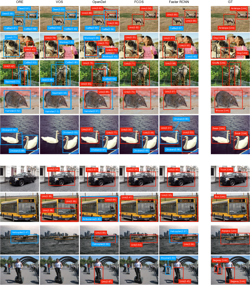
Figure 5: Examples of detection results for Open Images. Upper: the super-class is “Animal.” Lower: “Vehicle.” Red boxes represent unknown class detection, and blue boxes represent known class detection. “Unk” in the images stands for “unknown”.

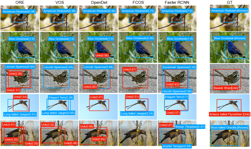
Figure 6: Examples of detection results for CUB200. See Fig 5 for notations.

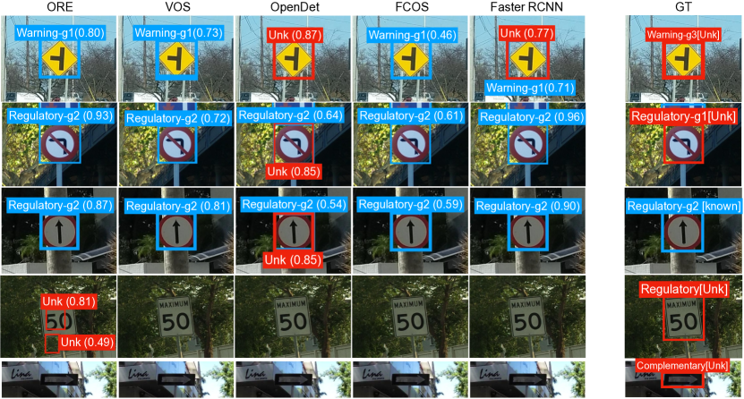
Figure 7: Examples of detection results for MTSD. See Fig 5 for notations.

References

- [1] A. Bansal, K. Sikka, G. Sharma, R. Chellappa, and A. Divakaran. Zero-Shot Object Detection. In Proc. ECCV, 2018.
- [2] A. Bendale and T. E. Boult. Towards Open Set Deep Networks. In Proc. CVPR, 2016.
- [3] N. Carion, F. Massa, G. Synnaeve, N. Usunier, A. Kirillov, and S. Zagoruyko. End-to-End Object Detection with Transformers. In Proc. ECCV, 2020.
- [4] K. Chen, J. Wang, J. Pang, Y. Cao, Y. Xiong, X. Li, S. Sun, W. Feng, Z. Liu, J. Xu, Z. Zhang, D. Cheng, C. Zhu, T. Cheng, Q. Zhao, B. Li, X. Lu, R. Zhu, Y. Wu, J. Dai, J. Wang, J. Shi, W. Ouyang, C. C. Loy, and D. Lin. MMDetection: Open MMLab Detection Toolbox and Benchmark. arXiv, 1906.07155, 2019.
- [5] J. Deng, W. Dong, R. Socher, L.-J. Li, K. Li, and L. Fei-Fei. ImageNet: A Large-Scale Hierarchical Image Database. In Proc. CVPR, 2009.
- [6] A. Dhamija, M. Gunther, J. Ventura, and T. Boult. The Overlooked Elephant of Object Detection: Open Set. In Proc. WACV, 2020.
- [7] X. Du, Z. Wang, M. Cai, and S. Li. VOS: Learning What You Don’t Know by Virtual Outlier Synthesis. In Proc. ICLR, 2022.
- [8] C. Ertler, J. Mislej, T. Ollmann, L. Porzi, and Y. Kuang. Traffic Sign Detection and Classification around the World. In Proc. ECCV, 2020.
- [9] M. Everingham, L. V. Gool, C. K. I. Williams, J. Winn, and A. Zisserman. The Pascal Visual Object Classes (VOC) Challenge. IJCV, 88(2):303–338, 2010.
- [10] C. Fellbaum. WordNet: An Electronic Lexical Database. Bradford Books, 1998.
- [11] P. F. Felzenszwalb, R. B. Girshick, D. McAllester, and D. Ramanan. Object Detection with Discriminatively Trained Part-Based Models. TPAMI, 32(9):1627–1645, 2010.
- [12] Y. Gal and Z. Ghahramani. Dropout as a Bayesian Approximation: Representing Model Uncertainty in Deep Learning. In Proc. ICML, 2016.
- [13] Z. Ge, S. Demyanov, and R. Garnavi. Generative OpenMax for Multi-Class Open Set Classification. In Proc. BMVC, 2017.
- [14] I. Goodfellow, J. Pouget-Abadie, M. Mirza, B. Xu, D. Warde-Farley, S. Ozair, A. Courville, and Y. Bengio. Generative Adversarial Nets. In Proc. NeurIPS, 2014.
- [15] A. Gupta, S. Narayan, K. J. Joseph, S. Khan, F. S. Khan, and M. Shah. OW-DETR: Open-World Detection Transformer. In Proc. CVPR, 2022.
- [16] J. Han, Y. Ren, J. Ding, X. Pan, K. Yan, and G.-S. Xia. Expanding Low-Density Latent Regions for Open-Set Object Detection. In Proc. CVPR, 2022.
- [17] K. He, X. Zhang, S. Ren, and J. Sun. Deep Residual Learning for Image Recognition. In Proc. CVPR, 2016.
- [18] K. J. Joseph, S. Khan, F. S. Khan, and V. N. Balasubramanian. Towards Open World Object Detection. In Proc. CVPR, 2021.
- [19] S. Kong and D. Ramanan. OpenGAN: Open-Set Recognition via Open Data Generation. In Proc. ICCV, 2021.
- [20] A. Kuznetsova, H. Rom, N. Alldrin, J. R. R. Uijlings, I. Krasin, J. Pont-Tuset, S. Kamali, S. Popov, M. Malloci, T. Duerig, and V. Ferrari. The Open Images Dataset V4: Unified image classification, object detection, and visual relationship detection at scale. arXiv, 1811.00982, 2018.
- [21] T.-Y. Lin, M. Maire, S. J. Belongie, L. D. Bourdev, R. B. Girshick, J. Hays, P. Perona, D. Ramanan, P. Dollár, and C. L. Zitnick. Microsoft COCO: Common Objects in Context. In Proc. ECCV, 2014.
- [22] T. Y. Lin, P. Dollar, R. Girshick, K. He, B. Hariharan, and S. Belongie. Feature Pyramid Networks for Object Detection. In Proc. CVPR, 2017.
- [23] C. Lu, R. Krishna, M. S. Bernstein, and L. Fei-Fei. Visual Relationship Detection with Language Priors. In Proc. ECCV, 2016.
- [24] D. Miller, F. Dayoub, M. Milford, and N. Sünderhauf. Evaluating Merging Strategies for Sampling-based Uncertainty Techniques in Object Detection. In Proc. ICRA, 2019.
- [25] D. Miller, L. Nicholson, F. Dayoub, and N. Sünderhauf. Dropout Sampling for Robust Object Detection in Open-Set Conditions. In Proc. ICRA, 2018.
- [26] L. Neal, M. Olson, X. Fern, W.-K. Wong, and F. Li. Open Set Learning with Counterfactual Images. In Proc. ECCV, 2018.
- [27] P. Oza and V. M. Patel. C2AE: Class Conditioned Auto-Encoder for Open-Set Recognition. In Proc. CVPR, 2019.
- [28] S. Ren, K. He, R. Girshick, and J. Sun. Faster R-CNN: Towards Real-time Object Detection with Region Proposal Networks. In Proc. NeurIPS, 2015.
- [29] W. J. Scheirer, A. de R. Rocha, A. Sapkota, and T. E. Boult. Toward Open Set Recognition. TPAMI, 35(7):1757–1772, 2013.
- [30] J. Shi and J. Malik. Normalized Cuts and Image Segmentation. TPAMI, 22(8):888–905, 2000.
- [31] L. Shu, H. Xu, and B. Liu. DOC: Deep Open Classification of Text Documents. In Proc. EMNLP, 2017.
- [32] D. K. Singh, S. N. Rai, K. J. Joseph, R. Saluja, V. N. Balasubramanian, C. Arora, A. Subramanian, and C. V. Jawahar. ORDER: Open World Object Detection on Road Scenes. In Proc. NeurIPS Workshops, 2021.
- [33] X. Sun, Z. Yang, C. Zhang, K.-V. Ling, and G. Peng. Conditional Gaussian Distribution Learning for Open Set Recognition. In Proc. CVPR, 2020.
- [34] Z. Tian, C. Shen, H. Chen, and T. He. FCOS: Fully Convolutional One-stage Object Detection. In Proc. ICCV, 2019.
- [35] S. Vaze, K. Han, A. Vedaldi, and A. Zisserman. Open-Set Recognition: A Good Closed-Set Classifier is All You Need. In Proc. ICLR, 2022.
- [36] V. Verma, A. Lamb, C. Beckham, A. Najafi, I. Mitliagkas, D. Lopez-Paz, and Y. Bengio. Manifold Mixup: Better Representations by Interpolating Hidden States. In Proc. ICML, 2019.
- [37] C. Wah, S. Branson, P. Welinder, P. Perona, and S. Belongie. Caltech-ucsd birds-200-2011. Technical Report CNS-TR-2011-001, California Institute of Technology, 2011.
- [38] Z. Wu, Y. Lu, X. Chen, Z. Wu, L. Kang, and J. Yu. UC-OWOD: Unknown-Classified Open World Object Detection. In Proc. ECCV, 2022.
- [39] R. Yoshihashi, W. Shao, R. Kawakami, S. You, M. Iida, and T. Naemura. Classification-Reconstruction Learning for Open-Set Recognition. In Proc. CVPR, 2019.
- [40] H. Zhang and V. M. Patel. Sparse Representation-based Open Set Recognition. TPAMI, 39(8):1690–1696, 2017.
- [41] X. Zhao, X. Liu, Y. Shen, Y. Qiao, Y. Ma, and D. Wang. Revisiting Open World Object Detection. arXiv, 2201.00471, 2022.
- [42] J. Zheng, W. Li, J. Hong, L. Petersson, and N. Barnes. Towards Open-Set Object Detection and Discovery. In Proc. CVPR Workshops, 2022.
- [43] D.-W. Zhou, H.-J. Ye, and D.-C. Zhan. Learning Placeholders for Open-Set Recognition. In Proc. CVPR, 2021.
- [44] X. Zhu, W. Su, L. Lu, B. Li, X. Wang, and J. Dai. Deformable DETR: Deformable Transformers for End-to-End Object Detection. In Proc. ICLR, 2021.