GIPSO: Geometrically Informed Propagation for Online Adaptation in 3D LiDAR Segmentation

Abstract

3D point cloud semantic segmentation is fundamental for autonomous driving. Most approaches in the literature neglect an important aspect, i.e., how to deal with domain shift when handling dynamic scenes. This can significantly hinder the navigation capabilities of self-driving vehicles. This paper advances the state of the art in this research field. Our first contribution consists in analysing a new unexplored scenario in point cloud segmentation, namely Source-Free Online Unsupervised Domain Adaptation (SF-OUDA). We experimentally show that state-of-the-art methods have a rather limited ability to adapt pre-trained deep network models to unseen domains in an online manner. Our second contribution is an approach that relies on adaptive self-training and geometric-feature propagation to adapt a pre-trained source model online without requiring either source data or target labels. Our third contribution is to study SF-OUDA in a challenging setup where source data is synthetic and target data is point clouds captured in the real world. We use the recent SynLiDAR dataset as a synthetic source and introduce two new synthetic (source) datasets, which can stimulate future synthetic-to-real autonomous driving research. Our experiments show the effectiveness of our segmentation approach on thousands of real-world point clouds. Code and synthetic datasets are available at https://github.com/saltoricristiano/gipso-sfouda.

1 Introduction

Autonomous driving requires accurate and efficient 3D visual scene perception algorithms. Low-level visual tasks such as detection and segmentation are crucial to enable higher-level tasks such as path planning [35, 11] and obstacle avoidance [46]. Deep learning-based methods have proven to be the most suitable option to meet these requirements so far, but at the cost of requiring large-scale annotated dataset for training [29]. Relying only on annotated data is not always a viable solution. This problem can be mitigated by considering synthetic data, as it can be generated at low cost with potentially unlimited annotations and under different environmental conditions [12, 23]. However, when a model trained on synthetic data is deployed in the real world, typically it will underperform due to domain shift, e.g., caused by varying lighting conditions, clutter, occlusions and materials with different reflective properties [56].

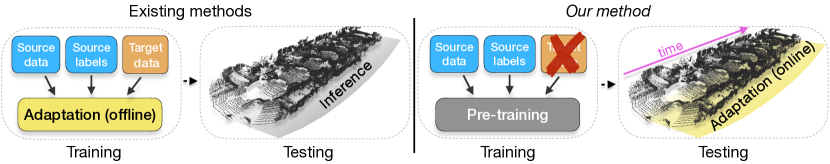
Figure 1: Existing methods adapt 3D semantic segmentation networks offline, requiring both source and target data. Differently, real-world applications urge solutions capable of adapting to unseen scenes online having access only to a pre-trained model.

We argue that a 3D semantic segmentation algorithm running on an autonomous vehicle should be capable of adapting online – handling scenarios that are visited for the first time while driving – and it should do so by only using the newly captured data. A variety of research works have addressed the adaptation problem in the context of 3D semantic segmentation. However, most approaches operate offline and assume to have access to training (source) data [28, 69, 63, 72, 73, 61]. In this paper, we argue that these two assumptions are too restrictive in an autonomous driving scenario (Fig. 1). On the one hand, offline adaptation would be equivalent to performing model adaptation on the data a vehicle has captured when the navigation has terminated, which is clearly a sub-optimal solution for autonomous driving [30]. On the other hand, having to rely on source data may not be a viable option, as it requires the method to store and query potentially large amount of data, thus hindering scalability [33, 36].

To overcome these limitations, in this paper we explore the new problem of Source-Free Online Unsupervised Domain Adaptation (SF-OUDA) for semantic segmentation, i.e., that of adapting a deep semantic segmentation model while a vehicle navigates in an unseen environment without relying on human supervision. Specifically, in this work we first implement, adapt and thoroughly analyze existing adaptation methods for the 3D semantic segmentation problem in a SF-OUDA setup. We experimentally observe that none of these methods provides consistent and satisfactory performance when employed in a SF-OUDA setting. However, there are elements of interest that, when carefully combined and extended, can be generally applicable. This leads us to move toward and design GIPSO (Geometrically Informed Propagation for Source-free Online adaptation), the first SF-OUDA method for 3D point cloud segmentation that builds upon recent advances in the literature, and exploits geometry information and temporal consistency to support the domain adaptation process. We also introduce two new synthetic datasets to benchmark SF-OUDA in two different real-world datasets, i.e. SemanticKITTI [3, 14, 13] and nuScenes [4]. We validate our approach on these new synthetic-to-real benchmarks. Our motivation for creating these datasets is to make evaluation more comprehensive and to assess the generalization ability of different techniques to different experimental setups. In summary, our contributions are:

• A thorough experimental analysis of existing domain adaptation methods for 3D semantic segmentation in a SF-OUDA setting;

• A novel method for SF-OUDA that exploits low-level geometric properties and temporal information to continuously adapt a 3D segmentation model;

• The introduction of two new LiDAR synthetic datasets that are compatible with the SemanticKITTI and nuScenes datasets.

2 Related work

Point cloud semantic segmentation. Point cloud segmentation methods can be classified into quantization-free and quantization-based architectures. The former processes the input point clouds in their original 3D format. Examples include PointNet [43] that is based on a series of multi layer perceptrons. PointNet++ [44] builds upon PointNet by using multi-scale sampling and neighbourhood aggregation to encode both global and local features. RandLA-Net [21] extends PoinNet++ [44] by embedding local spatial encoding, random sampling and attentive pooling. These methods are computationally inefficient when large-scale point clouds are used. The latter provides a computationally efficient alternative as input point clouds can be mapped into efficient representations, namely range maps [39, 60, 61], polar maps [67], 3D voxel grids [70, 17, 16, 8] or 3D cylindrical voxels [71]. Quantization-based approaches can be based on sparse convolutions [16, 17] or Minkowski convolutions [8]. We use the Minkowski Engine [8] as it provides a suitable trade off between accuracy and efficiency.

Unsupervised domain adaptation. Offline UDA can be performed either using source data [20, 37, 48, 72] or without using source data (source-free UDA) [36, 33, 49, 62]. Online UDA can be used to adapt a model to an unlabelled continuous target data stream through source domain supervision [58]. It can be employed for classification [40], image semantic segmentation [58], depth estimation [55, 68], robot manipulation [38], human mesh reconstruction [19] and occupancy mapping [54]. The assumption of unsupervised target input data can be relaxed and applied for online adaptation in classification [31], video-object segmentation [57] and motion planning [53]. Recently, test-time adaptation methods have been applied to online UDA in classification by using supervision from source data [52, 50, 59]. We tackle source-free online UDA for point cloud segmentation for the first time.

Domain adaptation for point cloud segmentation. Domain shift in point cloud segmentation occurs due to differences in (i) sampling noise, (ii) structure of the environment and (iii) class distributions [26, 61, 63, 69]. The domain adaptation problem can be formulated as a 3D surface completion task [63] or addressed with ray casting system capable of transferring the target sensor sampling pattern to the source data [28]. Other approaches tackle the domain adaptation problem in the synthetic-to-real setting (i.e., point cloud in the source domain are synthetic, while target ones are collected with LiDAR sensors) [60, 61, 69]. Attention models can be used to aggregate contextual information with large receptive fields at early layers of the model [60, 61]. Geodesic correlation alignment and progressive domain calibration can be also used to further improve domain adaptation effectiveness [61]. Authors in [69] argue that the method in [61] cannot be trained end-to-end as it employs a multi-stage pipeline. Therefore, they propose an end-to-end approach to simulate the dropout noise of real sensors on synthetic data through a generative adversarial network. Unlike these methods, we focus on SF-OUDA and propose a novel adaptation method which invokes geometry for propagating reliable pseudo-labels on target data.

Table 1: Comparison between public synthetic datasets and Synth4D in terms of sensor specifications, acquisition areas, number of scans, number of points, presence of odometry data, and whether the semantic classes are all or partially shared.

	Specifications		Areas	Scans	Points	Odometry	Shared semantic classes
Name	Sensor	FOV					S-KITTI [3]	nuScenes [4]
SinthCity [18]	MLS	360∘	city	1	367M		no	no
GTA-LiDAR [61]	HDL64E	90∘	town	121087	-		partial	no
PreSIL [23]	HDL64E	90∘	town	51074	3135M		partial	no
SynLiDAR [2]	HDL64E	360∘	city, town	198396	19482M		all	no
			harbor, rural
Synth4D (ours)	HDL64E	360∘	city, town	20000	2000M	✓	all	all
	HDL32E		rural, highway	20000	2000M

3 Datasets for synthetic-to-real adaptation

Autonomous driving simulators enable users to create ad-hoc synthetic datasets that can resemble real-world scenarios. Examples of popular simulators are GTA-V [64] and CARLA [12]. In principle, synthetic datasets should be compatible with their real-world counterpart [3, 4, 14], i.e., they should share the same semantic classes and the same sensor specifications, such as the resolution (32 vs. 64 channels) and the horizontal field of view (e.g., 90^∘ vs. 360^∘). However, this is not the case for most of the synthetic datasets in literature. The SynthCity [18] dataset contains large-scale point clouds that are generated from collections of several LiDAR scans, making it unsuitable for online domain adaptation as no odometry data is provided. PreSIL [23] and GTA-LiDAR’s [61] point clouds are captured from a moving vehicle using a simulated Velodyne HDL64E [34], as that of SemanticKITTI, however they are rendered with a different field of view, i.e., $90^{\circ}$ as opposed to $360^{\circ}$ of SemantiKITTI. SynLIDAR’s [2] point clouds are obtained using a simulated Velodyne HDL64E with $360^{\circ}$ field of view, as in SemantiKITTI. However, the odometry data is not provided, i.e., point clouds are all configured in their local reference frame. Therefore, domain adaptation algorithms that are based on ray-casting like [28] cannot be used.

To enable full compatibility with SemanticKITTI [3] and nuScenes [4], we present a new synthetic dataset, namely Synth4D, which we created using the CARLA simulator [12]. Tab. 1 compares Synth4D to the other synthetic datasets. Synth4D is composed of two sets of point cloud sequences, one compatible with SemanticKITTI and one compatible with nuScenes. Each set is composed of 20K labelled point clouds. Synth4D is captured using a vehicle navigating in four scenarios, i.e., town, highway, rural area and city. Because UDA requires consistent labels between source and target, we mapped the labels of Synth4D with those of SemanticKITTI/nuScenes using the original instructions given to annotators [3, 4], thus producing eight macro classes: vehicle, pedestrian, road, sidewalk, terrain, manmade, vegetation and unlabelled. Fig. 2 shows examples of annotated point clouds from Synth4D. See Supp. Mat. for more details.

\begin{overpic}[width=195.12767pt]{images/dataset/velohdl32e.jpg} \put(63.0,0.0){\color[rgb]{0,0,0}\scriptsize{(a)}} \end{overpic}

\begin{overpic}[width=195.12767pt]{images/dataset/velohdl64e.jpg} \put(67.0,0.0){\color[rgb]{0,0,0}\scriptsize{(b)}} \end{overpic}

\begin{overpic}[width=429.28616pt]{images/dataset/legend_h.pdf} \end{overpic}

Figure 2: Example of point clouds from Synth4D using the simulated Velodyne (a) HDL32E and (b) HDL64E.

4 SF-OUDA

We formulate the problem of SF-OUDA for 3D point cloud segmentation as follows. Given a deep network model $F_{\mathcal{S}}$ that is pre-trained with supervision on the source domain $\mathcal{S}$, we aim to adapt $F_{\mathcal{S}}$ on the target domain $\mathcal{T}$ given an unlabelled point cloud stream as input. $F_{\mathcal{S}}$ is pre-trained using the source data $\Gamma_{\mathcal{S}}=\{(X^{i}_{\mathcal{S}},Y^{i}_{\mathcal{S}})\}_{i=1}^{M_{\mathcal{S}}}$, where $X^{i}_{\mathcal{S}}$ is a synthetic point cloud, $Y^{i}_{\mathcal{S}}$ is the segmentation mask of $X^{i}_{\mathcal{S}}$ and $M_{\mathcal{S}}$ is the number of available synthetic point clouds. Let $X^{t}_{\mathcal{T}}$ be a point cloud of our stream at time $t$ and $F^{t}_{\mathcal{T}}$ be the target model adapted using $X^{t}_{\mathcal{T}}$ and $X^{t-w}_{\mathcal{T}}$, with $w>0$. $Y_{\mathcal{T}}$ is the set of unknown target labels and $C$ is the number of classes contained in $Y_{\mathcal{T}}$. The source classes and the target classes are coincident.

4.1 Our approach

The input to GIPSO is the point cloud $X^{t}_{\mathcal{T}}$ and an already processed point cloud $X^{t-w}_{\mathcal{T}}$. These point clouds are used to adapt $F_{\mathcal{S}}$ to $\mathcal{T}$ through self-supervision (Fig. 3). The input is processed by two modules. The first module aims to create labels for self-supervision by segmenting $X^{t}_{\mathcal{T}}$ with the source model $F_{\mathcal{S}}$. Because these labels are produced by an unsupervised deep network, we refer to them as pseudo-labels. We select a subset of segmented points that have reliable pseudo-labels through an adaptive selection criteria, and propagate them to less reliable points. The propagation uses geometric similarity in the feature space to increase the number of pseudo-labels available for self-supervision. To this end, we use an auxiliary deep network ($F_{aux}$) that is specialized in extracting geometrically-informed representations from 3D points. The second module aims to encourage temporal regularization of semantic information between $X^{t}_{\mathcal{T}}$ and $X^{t-w}_{\mathcal{T}}$. Unlike recent works [22], where a global point cloud descriptor of the scene is learnt, we exploit a self-supervised framework based on stop gradient [6] to ensure smoothness over time. Self-supervision through pseudo-label geometric propagation and temporal regularization are concurrently optimized to achieve the desired domain adaptation objective (Sec. 4.2).

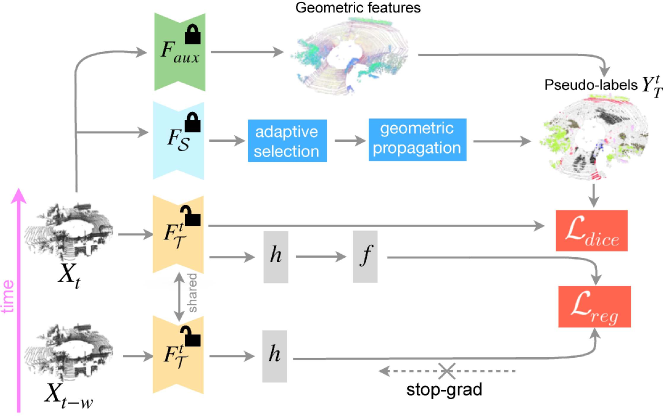
Figure 3: Overview of GIPSO. A source pre-trained model $F_{\mathcal{S}}$ selects seed pseudo-labels through our adaptive-selection approach. An auxiliary model $F_{aux}$ extracts geometric features to guide pseudo-label propagation. $\mathcal{L}_{dice}$ is minimised over the pseudo-labels $Y^{t}_{T}$. In parallel, semantic smoothness is enforced with $\mathcal{L}_{reg}$ over time. () frozen parameters. (

) learnable parameters.

Adaptive pseudo-label selection. An accurate selection of pseudo-labels is key to reliably adapt a model. In dynamic real-world scenarios, where new structures appear/disappear in/from the LiDAR field of view, traditional pseudo-labeling techniques [7, 51] can suffer from unexpected variations of class distributions, producing overconfident incorrect pseudo-labels and making more populated classes prevail on others [72, 73]. We overcome this problem by designing a class-balanced adaptive-thresholding strategy to choose reliable pseudo-labels. First, we compute an uncertainty index to filter out likely unreliable pseudo-labels. Second, we apply a different threshold for each class based on the uncertainty index distribution. This uncertainty index is directly related to the robustness of the output class distribution for each point. Robust pseudo-labels can be extracted from those points that consistently provide similar output distributions under different dropout perturbations [27]. We found that this approach works better than alternative confidence based approaches [72, 73].

Given the point cloud $X^{t}_{\mathcal{T}}$, we perform $J$ iterations of inference with $F_{\mathcal{S}}$ by using dropout and obtain

$$p_{\mathcal{T}}^{t}=\frac{1}{J}\sum_{j=1}^{J}p\left(F_{\mathcal{S}}|X_{\mathcal{T}}^{t},d_{j}\right),$$ (1)

where $p_{\mathcal{T}}^{t}$ is the averaged output distribution of $F_{\mathcal{S}}$ given $X_{\mathcal{T}}^{t}$ and $d_{j}$, i.e. the dropout at $j$-th iteration. We compute the uncertainty index $\nu_{\mathcal{T}}^{t}$ as the variance over the $C$ classes of $p_{\mathcal{T}}^{t}$ as

$$\nu_{\mathcal{T}}^{t}=E\left[\left(p_{\mathcal{T}}^{t}-\mu_{\mathcal{T}}^{t}\right)^{2}\right],$$ (2)

where $\mu_{\mathcal{T}}^{t}=E[p_{\mathcal{T}}^{t}]$ is the expected value of $p_{\mathcal{T}}^{t}$. Then, we select the least uncertain points by using a different uncertainty threshold for each class. Let $\lambda_{c}^{t}$ be the uncertainty threshold of class $c$ at time $t$. Since $\nu_{\mathcal{T}}^{t}$ defines the uncertainty for each point, we group $\nu_{\mathcal{T}}^{t}$ values per class and compute $\lambda_{c}^{t}$ as the $a$-th percentile of $\nu_{\mathcal{T}}^{t}$ for class $c$. Therefore, at time $t$ and for class $c$, we select only those pseudo-labels having the corresponding uncertainty index lower than $\lambda_{c}^{t}$ and use the corresponding pseudo-labels as seed pseudo-labels.

Geometric pseudo-label propagation. Typically, seed pseudo-labels are few and uninformative for the adaptation of the target model – the deep network is already confident about them. Therefore, we aim to propagate these pseudo-labels to potentially informative points. This is challenging because the model may drift during adaptation. We propose to use the features produced by an auxiliary geometrically-informed encoder $F_{aux}$ to propagate seed pseudo-labels to geometrically-similar points. Geometric features can be extracted using deep networks that compute 3D local descriptors [15, 1, 41]. 3D local descriptors are compact representations of local geometries with great generalization abilities across domains. Our intuition is that, while the propagation in the metric space may propagate only in the spatial neighborhood of seed pseudo-labels, the use of geometric features would allow us to propagate to geometrically similar points, which can be distant from their seeds in the metric space (Fig. 4).

Given a seed pseudo-labeled point $\tilde{\mathbf{x}}^{t}\in X^{t}_{\mathcal{T}}$, we compute a set of geometric similarities as

$$\mathcal{G}_{\tilde{\mathbf{x}}}^{t}=\lVert F_{aux}(\tilde{\mathbf{x}}^{t})-F_{aux}(X^{t}_{\mathcal{T}})\rVert_{2},$$ (3)

where $||\cdot||_{2}$ is the $l_{2}$-norm and $\mathcal{G}_{\tilde{\mathbf{x}}}^{t}$ is the set that contains the similarity values between $\tilde{\mathbf{x}}^{t}$ and all the other points of $X^{t}_{\mathcal{T}}$ (except $\tilde{\mathbf{x}}^{t}$). Then, we select the points that correspond to top $K$ values in $\mathcal{G}_{\tilde{\mathbf{x}}}^{t}$ and assign the pseudo-label of $\tilde{\mathbf{x}}^{t}$ to them. Let $Y^{t}_{\mathcal{T}}$ be the final set of pseudo-labels that we use for fine-tuning our model.

\begin{overpic}[width=117.07924pt]{images/method/propagation/propagation0.pdf} \put(10.0,-2.0){\color[rgb]{0,0,0}\scriptsize{(a)}} \end{overpic}

\begin{overpic}[width=134.42113pt]{images/method/propagation/propagation1.pdf} \put(10.0,-2.0){\color[rgb]{0,0,0}\scriptsize{(b)}} \end{overpic}

Figure 4: Example of geometric propagation: a) starting from seed pseudo-labels, b) geometric features are used to expand labels toward geometrically consistent regions.

Self-supervised temporal consistency loss. While the vehicle moves, the LiDAR sensor samples the environment from different viewpoints generating point clouds with different point distributions due to clutter and/or occlusions. As points of consecutive point clouds can be simply matched over time by using the vehicle’s odometry [14, 4], we can reasonably consider local variations of point distributions as local augmentations with the same semantic information. As a result, we can exploit recent self-supervised techniques to enforce temporal smoothness of our semantic features.

We begin by computing the set of corresponding points between $X^{t-w}_{\mathcal{T}}$ and $X^{t}_{\mathcal{T}}$ by using the vehicle’s odometry. Let $T_{t-w\rightarrow t}\in\mathbb{R}^{4\times 4}$ be the rigid transformation (from odometry) that maps $X^{t-w}_{\mathcal{T}}$ in the reference frame of $X^{t}_{\mathcal{T}}$. We define the set of corresponding point $\Omega^{t,t-w}$ as

$$\Omega^{t,t-w}= \left\{\{\mathbf{x}^{t}\in X^{t}_{\mathcal{T}},\mathbf{x}^{t-w}\in X^{t-w}_{\mathcal{T}}\}:\right.$$

$$\mathbf{x}^{t}=\mathtt{NN}\left(T_{t-w\rightarrow t}\circ\mathbf{x}^{t-w},X^{t}_{\mathcal{T}}\right),$$

$$\left.\lVert\mathbf{x}^{t}-\mathbf{x}^{t-w}\rVert_{2}<\tau\right\},$$ (4)

where $\mathtt{NN}(n,m)$ is the nearest-neighbour search given the set $m$ and the query $n$, $\circ$ is the operator that applies $T_{t-w\rightarrow t}$ to a 3D point and $\tau$ is a distance threshold.

We adapt the self-supervised learning framework proposed in SimSiam [6] to semantically smooth point clouds over time. We add an encoder network $h(\cdot)$ and a predictor head $f(\cdot)$ to the target model $F_{\mathcal{T}}$ and minimize the negative cosine similarity between consecutive semantic representations of corresponding points. Let $z^{t}\triangleq h(x^{t})$ be the encoder features over the target backbone for $x^{t}$ and let $q^{t}\triangleq f(h(x^{t}))$ be the respective predictor features. We minimize the negative cosine similarity as

$$\mathcal{D}_{t\rightarrow{t-w}}(q^{t},z^{t-w})=-\frac{q^{t}}{\left\|q^{t}\right\|_{2}}\cdot\frac{z^{t-w}}{\left\|z^{t-w}\right\|_{2}}$$ (5)

Time consistency is symmetric in the backward direction, hence we use the corresponding point of $x^{t}$ from $\Omega^{t,t-w}$ and define our self-supervised temporal consistency loss as

$$\mathcal{L}_{reg}=\frac{1}{2}\mathcal{D}_{t\rightarrow{t-w}}(q^{t},z^{t-w})+\frac{1}{2}\mathcal{D}_{t-w\rightarrow{t}}(q^{t-w},z^{t})$$ (6)

where stop-grad is applied on $z^{t}$ and $z^{t-w}$.

4.2 Online model update

Classes are typically highly unbalanced in each point cloud, e.g., a pedestrian class may be $1\%$ the number of points of the vegetation class. To this end, we use the soft Dice loss [25] as we found it works well when classes are unbalanced. Let $\mathcal{L}_{dice}$ be our soft Dice loss that uses the pseudo-labels selected though Eq. 3 as supervision. We define the overall adaptation objective as $\mathcal{L}_{tot}=\mathcal{L}_{dice}+\mathcal{L}_{reg}$, where $\mathcal{L}_{reg}$ is our regularization loss defined in Eq. 6.

5 Experiments

5.1 Experimental setup

Source and target datasets. We pre-train our source models on Synth4D and SynLiDAR [2], and validate our approach on the official validation sets of SemanticKITTI [3] and nuScenes [4] (target domains). In SemanticKITTI, we use the sequence $08$ that is composed of 4071 point clouds at 10Hz. In nuScenes, we use 150 sequences, each composed of 40 point clouds at 2Hz.

Implementation details. We use MinkowskiNet as deep network for point cloud segmentation [8]. We use ADAM: initial learning rate of $0.01$ with exponential decay, batch-size $16$ and weight decay $10^{-5}$. As auxiliary network $F_{aux}$, we use the PointNet-based architecture proposed in [41] trained on Synth4D that outputs a geometric features (descriptor) for a given 3D point. For online adaptation, we fix the learning rate to $10^{-3}$ and do not use schedulers as they would require prior knowledge about the stream length. Because we adapt our model on each new incoming point cloud, we use batch-size equal to $1$. We set $J$=5, $a$=1, $\tau$=0.3cm and use $0.5$ dropout probability. We set $K$=10, $w$=5 on SemanticKITTI, and $K$=5, $w$=1 on nuScenes. Parameters are the same in all the experiments.

Evaluation protocol. We follow the traditional evaluation procedure for online learning methods [5, 65], i.e., we evaluate the model performance on a new incoming frame using the model adapted up to the previous frame. We compute the Intersection over Union (IoU) [45] and report the average IoU (mIoU) improvement over the source (averaged over all the target sequences). We also evaluate the online version of our source model by fine-tuning it with ground-truth labels for all the points in the scene (target). We also evaluate the target upper bound (target) of our method obtained from the online finetuning of our source models over labelled target point clouds.

Table 2: Synth4D $\rightarrow$ SemanticKITTI online adaptation. Source: pre-trained source model (lower bound). We report absolute mIoU for Source and mIoU relative to Source for the other methods. Key. SF: Source-Free. UDA: Unsupervised DA. O: Online.

Model	SF	UDA	O	vehicle	pedestrian	road	sidewalk	terrain	manmade	vegetation	Avg
Source				63.90	12.60	38.10	47.30	20.20	26.10	43.30	35.93
Target	✓		✓	+16.84	+5.49	+8.48	+34.44	+51.92	+45.68	+39.09	+28.85
ADABN [32]	✓	✓		-7.80	-2.00	-10.20	-18.60	-7.70	+5.80	-0.70	-5.89
RayCast [28]		✓		+3.80	-2.60	-3.10	-0.50	+7.30	+4.50	+0.20	+1.37
ProDA∗	✓	✓	✓	-57.77	-12.34	-37.36	-46.95	-19.97	-25.62	-42.48	-34.64
SHOT∗	✓	✓	✓	-62.44	-12.00	-28.27	-40.20	-20.00	-25.47	-42.55	-32.99
ONDA [38]	✓	✓	✓	-13.60	-1.70	-10.60	-20.00	-7.10	+3.90	-5.10	-7.74
CBST∗	✓	✓	✓	-0.13	+0.58	-1.00	-1.12	+0.88	+1.69	+1.03	+0.28
TPLD∗	✓	✓	✓	+0.36	+1.18	-0.76	-0.71	+0.95	+1.74	+1.15	+0.56
GIPSO (Ours)	✓	✓	✓	+13.12	-0.54	+1.19	+2.45	+2.78	+5.64	+5.54	+4.31

5.2 Benchmarking existing methods for SF-OUDA

Because our approach is the first that specifically tackles SF-OUDA in the context of 3D point cloud segmentation, we perform an in-depth analysis of the literature to identify previous adaptation methods that can be re-purposed for SF-OUDA. Additionally, we experimentally evaluate their effectiveness on the considered datasets. We identify three categories of methods, as detailed below.

Batch normalization-based methods perform domain adaptation by considering different statistics for source and target samples within Batch Normalization (BN) layers. Here, we consider ADABN [32] and ONDA [38]. ADABN [32] is a source-free adaptation method which operates by updating the BN statistics assuming that all target data are available (offline adaptation). ONDA [38] is the online version of ADABN [32], where the target BN statistics are updated online based on the target data within a mini-batch. This can be regarded as a SF-OUDA method. However, these approaches are general-purpose methods and have not been previously evaluated for 3D point cloud segmentation.

Prototype-based adaptation methods use class centroids, i.e. prototypes, to generate target pseudo-labels that can be transferred to other samples via clustering. We implement SHOT [33] and ProDA [66]. SHOT [33] exploits Information Maximization (IM) to promote cluster compactness during offline adaptation. We implement SHOT by adapting the pre-trained model with the proposed IM loss online on each incoming target point cloud. ProDA [66] adopts a centroid-based weighting strategy to denoise target pseudo-labels, while also considering supervision from source data. We adapt ProDA to SF-OUDA by applying the same weighting strategy but removing source data supervision. We update target centroids at each incremental learning step. We refer to our SF-OUDA version of SHOT and PRODA as SHOT^∗ and ProDA^∗, respectively.

Self-training-based methods exploit source model predictions to adapt on the target domain by re-training the model. We implement CBST [72] and TPLD [51]. CBST [72] relies on a prediction confidence to select the most reliable pseudo labels. A confidence threshold is computed offline for each target class to avoid class unbalance. Our implementation of CBST, which we denote as CBST^∗, uses the same class balance selection strategy but updates the thresholds online on each incoming frame. Moreover, no source data are considered as we are in a SF-OUDA setting. TPLD [51], originally designed for 2D semantic segmentation, uses the pseudo-label selection mechanism in [72] but introduces a pixel pseudo label densification process. We implement TPLD by removing source supervision and replace the densification procedure with a 3D spatial nearest-neighbor propagation. Our version of TPLD is denoted as TPLD^∗.

Besides re-purposing existing approaches for SF-OUDA, we also evaluate an additional baseline, i.e. the rendering-based method RayCast [28]. This approach is based on the idea that target-like data can be obtained with photorealistic rendering applied to the source point clouds. Thus, adaptation is performed by simply training on target-like data. While RayCast can be regarded as an offline adapation approach, we select it as it only requires the parameters of the real sensor to obtain target-like data from source point clouds.

5.3 Results

Table 3: SynLiDAR $\rightarrow$ SemanticKITTI online adaptation. Source: pre-trained source model (lower bound). We report absolute mIoU for Source and mIoU relative to Source for the other methods. Key. SF: Source-Free. UDA: Unsupervised DA. O: Online.

Model	SF	UDA	O	vehicle	pedestrian	road	sidewalk	terrain	manmade	vegetation	Avg
Source				59.80	14.20	34.90	53.50	31.00	37.40	50.50	40.19
Target	✓		✓	+21.32	+8.09	+11.51	+28.13	+40.46	+33.67	+30.63	+24.83
ADABN [32]	✓	✓		+3.90	-6.40	-0.20	-3.70	-5.70	+1.40	+0.30	-1.49
RayCast [28]		✓		-	-	-	-	-	-	-	-
ProDA∗	✓	✓	✓	-53.30	-13.79	-33.83	-52.78	-30.52	-36.68	-49.29	-38.60
SHOT∗	✓	✓	✓	-57.83	-12.64	-24.80	-46.02	-30.80	-36.83	-49.32	-36.89
ONDA [38]	✓	✓	✓	-2.90	-6.40	-2.20	-8.80	-7.60	-1.20	-6.70	-5.11
CBST∗	✓	✓	✓	+0.99	-0.83	+0.55	+0.20	+0.74	-0.07	+0.38	+0.28
TPLD∗	✓	✓	✓	+0.90	-0.48	+0.59	+0.33	+0.84	+0.07	+0.37	+0.37
GIPSO (Ours)	✓	✓	✓	+13.95	-6.76	+3.26	+5.01	+3.00	+3.34	+4.08	+3.70

Table 4: Synth4D $\rightarrow$ nuScenes online adaptation. Source: pre-trained source model (lower bound). We report absolute mIoU for Source and mIoU relative to Source for the other methods. Key. SF: Source-Free. UDA: Unsupervised DA. O: Online.

Model	SF	UDA	O	vehicle	pedestrian	road	sidewalk	terrain	manmade	vegetation	Avg
Source				22.54	14.38	42.03	28.39	15.58	38.18	54.14	30.75
Target	✓		✓	+3.76	+0.92	+9.41	+16.95	+19.79	+10.92	+10.71	+10.35
ADABN [32]	✓	✓		+1.23	-2.74	-1.24	+0.14	+0.53	+0.70	+4.03	+0.38
RayCast [28]		✓		-1.36	-9.69	-3.53	-3.42	-2.77	-2.54	-0.91	-3.46
ProDA∗	✓	✓	✓	+0.57	-1.40	+0.73	+0.09	+0.71	+0.40	+0.91	+0.29
SHOT∗	✓	✓	✓	+0.82	-1.77	+0.68	-0.05	-0.70	-0.54	+1.09	-0.07
ONDA [38]	✓	✓	✓	+0.34	-1.90	-1.19	-0.62	+0.18	-0.40	+0.58	-0.43
CBST∗	✓	✓	✓	+0.37	-2.61	-1.35	-0.79	+0.19	-0.36	-0.45	-0.71
TPLD∗	✓	✓	✓	+0.65	-1.90	-0.96	-0.39	+0.43	+0.07	+0.86	-0.18
GIPSO (Ours)	✓	✓	✓	+0.55	-3.76	+1.64	+1.72	+2.28	+1.18	+2.36	+0.85

Evaluating GIPSO. Tab. 2, 3 and 4 report the results of our quantitative evaluation in the cases of Synth4D $\rightarrow$ SemanticKITTI, Synlidar $\rightarrow$ SemanticKITTI and Synth4D $\rightarrow$ nuScenes, respectively. The numbers in the tables indicate the improvement over the source model. GIPSO achieves an average IoU improvement of +4.31 on Synth4D $\rightarrow$ SemanticKITTI, +3.70 on Synlidar $\rightarrow$ SemanticKITTI and +0.85 on Synth4D $\rightarrow$ nuScenes. GIPSO outperforms both offline and online methods by a large margin on Synth4D $\rightarrow$ SemanticKITTI and Synlidar $\rightarrow$ SemanticKITTI, while it achieves a lower improvement over Synth4D $\rightarrow$ nuScenes. On SemanticKITTI, GIPSO can effectively improve road, sidewalk, terrain, manmade and vegetation. vehicle is the best performing class, which can achieve a mIoU above +13. pedestrian is the worst performing class on all the datasets. pedestrian is a challenging class because it is significantly unbalanced compared to the others, also in the source domain. Although we attempted to mitigate the problem of unbalanced classes using adaptive thresholding and soft Dice loss, there are still situations that are difficult to address (see Sec. 6 for details). On nuScenes, the improvement is minor because at its lower resolutions makes patterns less distinguishable and more difficult to segment.

Evaluating state-of-the-art methods. We also analyze the performance of the existing methods discussed in Sec. 5.2. Batch-normalisation based methods perform poorly on all the datasets, with only ADABN [32] showing a minor improvement on nuScenes. We argue that non-i.i.d. batch samples arising in the online setting are playing an important role in this degradation, as they can have detrimental effects on models with BN layers [24]. SHOT^∗ and ProDA^∗ perform poorly in almost all the experiments, except on Synth4D $\rightarrow$ nuScenes where ProDA^∗ achieves +0.29. This minor improvement may be due to the short sequences of nuScenes (40 frames) making centroids less likely to drift. This does not occur in SemanticKITTI where the long sequence causes a rapid drift (see detailed in Sec. 5.4). CBST^∗ and TPLD^∗ improve on SemanticKITTI and perform poorly on nuScenes. This can be ascribed to the noisy pseudo-labels that are selected using their confidence-based filtering approach. Lastly, RayCast [28] achieves +1.37 on Synth4D $\rightarrow$ SemanticKITTI, but underperform on Synth4D $\rightarrow$ nuScenes with a degradation of -3.46. RayCast was originally proposed for real-to-real adaptation, therefore we believe that its performance may be affected by the large difference in point cloud resolution between Synth4D and nuScenes. RayCast underperforms GIPSO in the online setup, thus showing how offline solutions can fail in dynamic domains. Note that RayCast cannot be evaluated using Synlidar, because Synlidar does not provide odometry information.

5.4 In-depth analyses

Ablation study. Tab. 6 shows the results of our ablation study on Synth4D $\rightarrow$ SemanticKITTI. When we use only the adaptive pseudo-label selection (A) we can achieve +1.07 compared to the source. When we combine A with the temporal regularization (T) we can further improve by +3.65. Then we can achieve our best performance through the geometric propagation (P) of the pseudo labels.

\begin{overpic}[width=208.13574pt]{images/method/per_class_improvement.pdf} \put(-4.0,15.0){\color[rgb]{0,0,0}\tiny\rotatebox{90.0}{mIoU improvement}} \put(79.0,-4.0){\color[rgb]{0,0,0}\tiny Time} \put(80.0,-13.0){\color[rgb]{0,0,0}\scriptsize{(a)}} \end{overpic}

\begin{overpic}[width=212.47617pt]{images/method/db_index.pdf} \put(-2.0,30.0){\color[rgb]{0,0,0}\tiny\rotatebox{90.0}{DB-Index}} \put(79.0,-4.0){\color[rgb]{0,0,0}\tiny Time} \put(80.0,-13.0){\color[rgb]{0,0,0}\scriptsize{(b)}} \end{overpic}

Figure 5: (a) Per-class improvement of GIPSO over time on Synth4D$\rightarrow$SemanticKITTI. (b) DB-Index over time on Synth4D$\rightarrow$SemanticKITTI. The lower the DB-Index, the better the class separation of the features.

Oracle study. We analyze the importance of using a reliable pseudo-label selection metric. Tab. 6 shows the pseudo-label accuracy as a function of the points that are selected as the $K$-th best candidates based on the distance from their centroids (as proposed in [66]), confidence (as proposed in [72]) and uncertainty (ours). Centroid-based selection shows a low accuracy even at $K=1$, which tends to worsen as $K$ increases. Confidence-based selection is more reliable than the centroid-based selection. We found uncertainty-based selection to be more reliable at smaller values of $K$, which we deem to be more important than having more pseudo-labels but less reliable.

Table 5: Synth4D$\rightarrow$SemanticKITTI ablation study of GIPSO: (A) Adaptive thresholding; (A+T) A + Temporal consistency; (A+T+P) A+T + geometric Propagation.

Source	Target	A	A+T	A+T+P
35.95	+28.85	+1.07	+3.65	+4.31

Table 6: Oracle study on Synth4D $\rightarrow$ SemanticKITTI that compares the accuracy of different pseudo-label selection metrics: Centroid, Confidence and Uncertainty.

	Centroid	Confidence	Uncertainty
Top-1	38.1	66.7	76.1
Top-10	43.8	61.4	69.7

Per-class temporal behavior. Fig. 5a shows the mIoU over time for each class on Synth4D $\rightarrow$ SemanticKITTI. We can observe that six out of seven classes have a steady improvement: vehicle is the best performing class, followed by vegetation and manmade. Drops in mIoU are typically due to sudden geometric variations of the point cloud, e.g., a road junction after a straight road, or a jammed road after a empty road. pedestrian confirms to be the most challenging class.

Temporal compactness of features. We assess how well points are organized in the feature space over time. We use the DB Index (DBI) that is typically used in clustering to measures the feature intra- and inter-class distances [10]. The lower the DBI, the better the quality of the features. We use SHOT^∗ and ProDA^∗ as comparisons with our method, and the source and target models as references. Fig. 5b shows the DBI variations over time. SHOT^∗ behavior is typical of a drift, as features of different classes become interwoven. ProDA^∗ does not drift, but it produces features that are worse than the source model. Our approach is between source and target models, with a tendency to get closer to target.

Different 3D local descriptors. We assess the effectiveness of different 3D local descriptors. We test FPFH [47] (handcrafted) and FCGF [9] (deep learning) descriptors. GIPSO achieves +3.56 mIoU with FPFH, +4.12 mIoU with FCGF and +4.31 mIoU with DIP. This is inline with the experiments shown in [42], where DIP shows a superior generalization capability across domains than FCGF.

Performance with global features. We assess the GIPSO performance on Synth4D$\rightarrow$SemanticKITTI when the global temporal consistency loss proposed in STRL [22] is used instead of our per-point loss (Eq. 5). This variation achieves $+1.74$ mIoU, showing that per-point temporal consistency is key.

Qualitative results. Fig. 6 shows the comparison between GIPSO and the source model on on Synth4D$\rightarrow$SemanticKITTI. The first row shows frame $178$ of SemanticKITTI with an improvement of $+27.14$ mIoU (large). The classes vehicle, sidewalk and terrain are incorrectly segmented by the source model, we can see a significant improvement in segmentation on these classes after adaptation. The second and third rows show frame $1193$ and frame $2625$ with an improvement of $+10.00$ mIoU (medium) and $+4.99$ mIoU (small). Improvements are visible after adaptation in the classes vehicle, sidewalk and road. The last row shows a segmentation drift for road that is caused by incorrect pseudo-labels.

\begin{overpic}[width=195.12767pt]{images/results/high/high_source.pdf} \put(65.0,85.0){\color[rgb]{0,0,0}\footnotesize{source}} \put(-8.0,35.0){\color[rgb]{0,0,0}\footnotesize\rotatebox{90.0}{{large}}} \end{overpic}	\begin{overpic}[width=195.12767pt]{images/results/high/high_adapted.pdf} \put(65.0,85.0){\color[rgb]{0,0,0}\footnotesize{ours} } \end{overpic}
\begin{overpic}[width=195.12767pt]{images/results/medium/medium_source.pdf} \put(-8.0,30.0){\color[rgb]{0,0,0}\footnotesize\rotatebox{90.0}{{medium}}} \end{overpic}	\begin{overpic}[width=195.12767pt]{images/results/medium/medium_adapted.pdf} \end{overpic}
\begin{overpic}[width=195.12767pt]{images/results/low/low_source.pdf} \put(-8.0,30.0){\color[rgb]{0,0,0}\footnotesize\rotatebox{90.0}{{small}}} \end{overpic}	\begin{overpic}[width=195.12767pt]{images/results/low/low_adapted.pdf} \end{overpic}

\begin{overpic}[width=433.62pt]{images/dataset/legend_h.pdf} \end{overpic}

Figure 6: Results on Synth4D$\rightarrow$SemanticKITTI with three different ranges of mIoU improvements, i.e., large (+27.2), medium (+10.0) and small (+5.1).

6 Discussions

Conclusions. We studied for the first time the problem of SF-OUDA for 3D point cloud segmentation in a synthetic-to-real setting. We experimentally showed that existing approaches do not suffice in coping with domain shift in this scenario. We presented GIPSO that relies on adaptive self-training and geometric-features propagation to address SF-OUDA. We also introduced a novel synthetic dataset, namely Synth4D composed of two splits and matching the sensor setup of SemanticKITTI and nuScenes, respectively. Experiments on three different benchmarks showed that GIPSO outperforms state-of-the-art approaches.

Limitations. GIPSO limitations are related to geometric propagation and long-tailed classes. If objects of different classes share similar geometric structures, the geometric propagation may be deleterious. This can be mitigated by using another sensor modality (e.g. RGB) or by accounting for multi-scale signals to exploit context information. If severe class unbalance occurs, semantic segmentation accuracy may be affected, e.g. pedestrian class in Tabs. 2-4. This can be mitigated by re-weighting the loss through a class-balanced term (computed on the source).

Acknowledgments. This work was partially supported by OSRAM GmbH, by the Italian Ministry of Education, Universities and Research (MIUR) “Dipartimenti di Eccellenza 2018-2022”, by the EU JPI/CH SHIELD project, by the PRIN project PREVUE (Prot. 2017N2RK7K), the EU ISFP PROTECTOR (101034216) project and the EU H2020 MARVEL (957337) project and, it was carried out in the Vision and Learning joint laboratory of FBK and UNITN.

References

- [1] Ao, S., Hu, Q., Yang, B., Markham, A., Guo, Y.: SpinNet: Learning a General Surface Descriptor for 3D Point Cloud Registration. In: CVPR (2021)
- [2] Aoran, X., Jiaxing, H., Dayan, G., Fangneng, Z., Shijian, L.: Synlidar: Learning from synthetic lidar sequential point cloud for semantic segmentation. arXiv (2021)
- [3] Behley, J., Garbade, M., Milioto, A., Quenzel, J., Behnke, S., Stachniss, C., Gall, J.: SemanticKITTI: A Dataset for Semantic Scene Understanding of LiDAR Sequences. In: ICCV (2019)
- [4] Caesar, H., Bankiti, V., Lang, A., Vora, S., Liong, V., Xu, Q., Krishnan, A., Pan, Y., Baldan, G., Beijbom, O.: nuScenes: A multimodal dataset for autonomous driving. In: CVPR (2020)
- [5] Cesa-Bianchi, N., Conconi, A., Gentile, C.: On the generalization ability of on-line learning algorithms. T-IT (2004)
- [6] Chen, X., He, K.: Exploring simple siamese representation learning. In: CVPR (2021)
- [7] Chen, Y., Li, W., Sakaridis, C., Dai, D., van Gool, L.: Domain adaptive faster r-cnn for object detection in the wild. In: CVPR (2018)
- [8] Choy, C., Gwak, J., Savarese, S.: 4d spatio-temporal convnets: Minkowski convolutional neural networks. In: CVPR (2019)
- [9] Choy, C., Park, J., Koltun, V.: Fully convolutional geometric features. In: ICCV (2019)
- [10] Davies, D., Bouldin, D.: A cluster separation measure. T-PAMI (1979)
- [11] Dolgov, D., Thrun, S., Montemerlo, M., Diebel, J.: Path planning for autonomous vehicles in unknown semi-structured environments. IJRR (2010)
- [12] Dosovitskiy, A., Ros, G., Codevilla, F., Lopez, A., Koltun, V.: CARLA: An open urban driving simulator. In: ACRL (2017)
- [13] Geiger, A., Lenz, P., Stiller, C., Urtasun, R.: Vision meets robotics: The KITTI dataset. IJRR (2013)
- [14] Geiger, A., Lenz, P., Urtasun, R.: Are we ready for autonomous driving? The KITTI vision benchmark suite. In: CVPR (2012)
- [15] Gojcic, Z., Zhou, C., Wegner, J., Andreas, W.: The perfect match: 3D point cloud matching with smoothed densities. In: CVPR (2019)
- [16] Graham, B., Engelcke, M., van der Maaten, L.: 3d semantic segmentation with submanifold sparse convolutional networks. In: CVPR (2018)
- [17] Graham, B., van der Maaten, L.: Submanifold sparse convolutional networks. arXiv (2017)
- [18] Griffiths, D., Boehm, J.: SynthCity: A large scale synthetic point cloud. In: arXiv (2019)
- [19] Guan, S., Xu, J., Wang, Y., Ni, B., Yang, X.: Bilevel online adaptation for out-of-domain human mesh reconstruction. In: CVPR (2021)
- [20] Hoffman, J., Tzeng, E., Park, T., Zhu, J., Isola, P., Saenko, K., Efros, A., Darrell, T.: Cycada: Cycle-consistent adversarial domain adaptation. In: ICML (2018)
- [21] Hu, Q., Yang, B., Xie, L., Rosa, S., Guo, Y., Wang, Z., Trigoni, N., Markham, A.: RandLA-Net: Efficient semantic segmentation of large-scale point clouds. In: CVPR (2020)
- [22] Huang, S., Xie, Y., Zhu, S., Zhu, Y.: Spatio-temporal self-supervised representation learning for 3d point clouds. In: ICCV (2021)
- [23] Hurl, B., Czarnecki, K., Waslander, S.: Precise synthetic image and lidar (PreSIL) dataset for autonomous vehicle perception. In: IVS (2019)
- [24] Ioffe, S.: Batch renormalization: Towards reducing minibatch dependence in batch-normalized models. arXiv (2017)
- [25] Jadon, S.: A survey of loss functions for semantic segmentation. In: CIBCB (2020)
- [26] Jaritz, M., Vu, T.H., de Charette, R., Wirbel, E., Pérez, P.: xMUDA: Cross-modal unsupervised domain adaptation for 3d semantic segmentation. In: CVPR (2020)
- [27] Kendall, A., Badrinarayanan, V., Cipolla, R.: Bayesian segnet: Model uncertainty in deep convolutional encoder-decoder architectures for scene understanding. In: BMVC (2017)
- [28] Langer, F., Milioto, A., Haag, A., Behley, J., Stachniss, C.: Domain transfer for semantic segmentation of LiDAR data using deep neural networks. In: IROS (2021)
- [29] LeCun, Y., Bengio, Y., Hinton, G.: Deep learning. Nature (2015)
- [30] Levinson, J., et al.: Towards fully autonomous driving: Systems and algorithms. In: IV (2011)
- [31] Li, D., Hospedales, T.: Online meta-learning for multi-source and semi-supervised domain adaptation. In: ECCV (2020)
- [32] Li, Y., Wang, N., Shi, J., Liu, J., Hou, X.: Revisiting batch normalization for practical domain adaptation. arXiv (2016)
- [33] Liang, J., Hu, D., Feng, J.: Do we really need to access the source data? source hypothesis transfer for unsupervised domain adaptation. In: ICML (2020)
- [34] Lidar, V.: VelodyneLidar. https://velodynelidar.com (2021)
- [35] Liu, C., Lee, S., Varnhagen, S., Tseng, H.: Path planning for autonomous vehicles using model predictive control. In: IV (2017)
- [36] Liu, Y., Zhang, W., Wang, J.: Source-free domain adaptation for semantic segmentation. In: CVPR (2021)
- [37] Long, M., Cao, Z., Wang, J., Jordan, M.: Conditional adversarial domain adaptation. In: NeurIPS (2018)
- [38] Mancini, M., Karaoguz, H., Ricci, E., Jensfelt, P., Caputo, B.: Kitting in the wild through online domain adaptation. In: IROS (2018)
- [39] Milioto, A., Vizzo, I., Behley, J., Stachniss, C.: Rangenet++: Fast and accurate lidar semantic segmentation. In: IROS (2019)
- [40] Moon, J., Das, D., Lee, C.: Multi-step online unsupervised domain adaptation. In: ICASSP (2020)
- [41] Poiesi, F., Boscaini, D.: Distinctive 3D local deep descriptors. In: ICPR (2021)
- [42] Poiesi, F., Boscaini, D.: Learning general and distinctive 3D local deep descriptors for point cloud registration. T-PAMI (2022)
- [43] Qi, C., Su, H., Mo, K., Guibas, L.: Pointnet: Deep learning on point sets for 3d classification and segmentation. In: CVPR (2017)
- [44] Qi, C., Yi, L., Su, H., Guibas, L.: Pointnet++: Deep hierarchical feature learning on point sets in a metric space. arXiv (2017)
- [45] Rahman, M., Wang, Y.: Optimizing intersection-over-union in deep neural networks for image segmentation. In: ISVC (2016)
- [46] Rosolia, U., Bruyne, S.D., Alleyne, A.: Autonomous vehicle control: A nonconvex approach for obstacle avoidance. T-CST (2016)
- [47] Rusu, R., Blodow, N., Beetz, M.: Fast point feature histograms (FPFH) for 3D registration. In: ICRA (2009)
- [48] Saito, K., Watanabe, K., Ushiku, Y., Harada, T.: Maximum classifier discrepancy for unsupervised domain adaptation. In: CVPR (2018)
- [49] Saltori, C., Lathuiliére, S., Sebe, N., Ricci, E., Galasso, F.: Sf-uda3d: Source-free unsupervised domain adaptation for lidar-based 3d object detection. arXiv (2020)
- [50] Schneider, S., Rusak, E., Eck, L., Bringmann, O., Brendel, W., Bethge, M.: Improving robustness against common corruptions by covariate shift adaptation. NeurIPS (2020)
- [51] Shin, I., Woo, S., Pan, F., Kweon, I.: Two-phase pseudo label densification for self-training based domain adaptation. In: ECCV (2020)
- [52] Sun, Y., Wang, X., Liu, Z., Miller, J., Efros, A., Hardt, M.: Test-time training with self-supervision for generalization under distribution shifts. In: ICML (2020)
- [53] Tanneberg, D., Peters, J., Rueckert, E.: Efficient online adaptation with stochastic recurrent neural networks. In: Humanoids (2017)
- [54] Tompkins, A., Senanayake, R., Ramos, F.: Online domain adaptation for occupancy mapping. arXiv (2020)
- [55] Tonioni, A., Tosi, F., Poggi, M., Mattoccia, S., Stefano, L.D.: Real-time self-adaptive deep stereo. In: CVPR (2019)
- [56] Torralba, A., Efros, A.: Unbiased look at dataset bias. In: CVPR (2011)
- [57] Voigtlaender, P., Leibe, B.: Online adaptation of convolutional neural networks for video object segmentation. arXiv (2017)
- [58] Volpi, R., Jorge, P.D., Larlus, D., Csurka, G.: On the road to online adaptation for semantic image segmentation. In: CVPR (2022)
- [59] Wang, D., Shelhamer, E., Liu, S., Olshausen, B., Darrell, T.: Tent: Fully test-time adaptation by entropy minimization. ICLR (2021)
- [60] Wu, B., Wan, A., Yue, X., Keutzer, K.: Squeezeseg: Convolutional neural nets with recurrent crf for real-time road-object segmentation from 3d lidar point cloud. In: ICRA (2018)
- [61] Wu, B., Zhou, X., Zhao, S., Yue, X., Keutzer, K.: Squeezesegv2: Improved model structure and unsupervised domain adaptation for road-object segmentation from a lidar point cloud. In: ICRA (2019)
- [62] Yang, S., van de Weijer, J., Herranz, L., Jui, S., et al.: Exploiting the intrinsic neighborhood structure for source-free domain adaptation. NeurIPS (2021)
- [63] Yi, L., Gong, B., Funkhouser, T.: Complete & label: A domain adaptation approach to semantic segmentation of lidar point clouds. arXiv (2021)
- [64] Yue, X., Wu, B., Seshia, S., Keutzer, K., Sangiovanni-Vincentelli, A.: A LiDAR point cloud generator: from a virtual world to autonomous driving. In: ICMR (2018)
- [65] Zhan, X., Xie, J., Liu, Z., Ong, Y., Loy, C.: Online deep clustering for unsupervised representation learning. In: CVPR (2020)
- [66] Zhang, P., Zhang, B., Zhang, T., Chen, D., Wang, Y., Wen, F.: Prototypical pseudo label denoising and target structure learning for domain adaptive semantic segmentation. In: CVPR (2021)
- [67] Zhang, Y., Zhou, Z., David, P., Yue, X., Xi, Z., Gong, B., Foroosh, H.: Polarnet: An improved grid representation for online lidar point clouds semantic segmentation. In: CVPR (2020)
- [68] Zhang, Z., Lathuilière, S., Pilzer, A., Sebe, N., Ricci, E., Yang, J.: Online adaptation through meta-learning for stereo depth estimation. arXiv (2019)
- [69] Zhao, S., Wang, Y., Li, B., Wu, B., Gao, Y., Xu, P., Darrell, T., Keutzer, K.: epointda: An end-to-end simulation-to-real domain adaptation framework for lidar point cloud segmentation. arXiv (2020)
- [70] Zhou, Y., Tuzel, O.: Voxelnet: End-to-end learning for point cloud based 3d object detection. In: CVPR (2018)
- [71] Zhu, X., Zhou, H., Wang, T., Hong, F., Ma, Y., Li, W., Li, H., Lin, D.: Cylindrical and asymmetrical 3d convolution networks for lidar segmentation. In: CVPR (2021)
- [72] Zou, Y., Yu, Z., Kumar, B., Wang, J.: Unsupervised domain adaptation for semantic segmentation via class-balanced self-training. In: ECCV (2018)
- [73] Zou, Y., Yu, Z., Liu, X., Kumar, B., Wang, J.: Confidence regularized self-training. In: ICCV (2019)