On the rotation curve of disk galaxies in General Relativity

Abstract

Recently, it has been suggested that the phenomenology of flat rotation curves observed at large radii in the equatorial plane of disk galaxies can be explained as a manifestation of General Relativity instead of the effect of Dark Matter halos. In this paper, by using the well known weak field, low velocity gravitomagnetic formulation of GR, the expected rotation curves in GR are rigorously obtained for purely baryonic disk models with realistic density profiles, and compared with the predictions of newtonian gravity for the same disks in absence of Dark Matter. As expected, the resulting rotation curves are indistinguishable, with GR corrections at all radii of the order of $v^{2}/c^{2}\approx 10^{-6}$. Next, the gravitomagnetic Jeans equations for two-integral stellar systems are derived, and then solved for the Miyamoto-Nagai disk model, showing that finite-thickness effects do not change the previous conclusions. Therefore, the observed phenomenology of galactic rotation curves at large radii requires Dark Matter in GR exactly as in newtonian gravity, unless the cases here explored are reconsidered in the full GR framework with substantially different results (with the surprising consequence that the weak field approximation of GR cannot be applied to the study of rotating systems in the weak field regime). In the paper, the mathematical framework is described in detail, so that the present study can be extended to other disk models, or to elliptical galaxies (where Dark Matter is also required in newtonian gravity, but their rotational support can be much less than in disk galaxies).

1. Introduction

Recently, following the original suggestion of Cooperstock and Tieu (2007, see also Balasin and Grumiller 2008), several papers addressed the interesting possibility that the observed phenomenology of rotation curves in disk galaxies can be explained by General Relativity effects (hereafter, GR) peculiar of rotating systems, without the need to invoke the presence of Dark Matter (hereafter DM) halos in order to produce the flat behavior at large galactocentric distances.

Unfortunately, no definite consensus about the importance of GR effects on the rotation curve of disk galaxies seems to be reached, with widely different conclusions ranging from support to the hypothesis, to the identification of possible mathematical issues affecting the disk models used to compute the GR solutions (for a representative, but almost certainly incomplete list of papers representing the different positions, see, e.g., Korzynski 2005, Vogt and Letelier 2005a,b, Cross 2006, Fuchs and Phleps 2006, Crosta et al. 2020, Carrick and Cooperstock 2012, Deledicque 2019, Ludwig 2021, 2022, Ruggiero et al. 2021, Toth 2021, Astesiano and Ruggiero 2022, and references therein).

If confirmed, the suggestion above would be a most surprsing result, with consequences extending well beyond the problem of the interpretation of galaxy rotation curves, and perhaps even beyond the problem of the existence of DM. A list of some of these consequences (not necessarily in order of importance) is the following: 1) usually, it is expected that lowest order corrections of GR to newtonian dynamics are of the order of $v^{2}/c^{2}$, where $v$ is a characteristic velocity associated with the newtonian gravitational potential of the system, and $c$ is the speed of light. In astronomical systems where the presence of DM is required by newtonian gravity, $v/c\approx 10^{-3}$ or less, therefore such systems are empirically in the GR weak field regime. If the flat region of rotation curves is a GR effect, then we face the problem of explaining in physical terms how an expected effect of the order of $\approx 10^{-6}$ actually becomes more important than the zeroth-order newtonian term: we notice that mathematically such a behavior characterizes singular perturbation theory. 2) In case the previous point is satisfactorily answered, we should then explain why other effects of GR in the weak field approximation (not directly related to rotation) remain at the level of small perturbations, for example by requiring the presence of DM in order to reproduce gravitational lensing, and correctly predicting the small amount of planetary precession left unexplaied once newtonian precession is considered. 3) DM is clearly required by newtonian gravity not only in rotating disk galaxies, but also in velocity dispersion (pressure) supported astronomical systems with low ordered rotation, such as elliptical galaxies and cluster of galaxies (with converging predictions about the structural properties of the inferred DM halos obtained from different diagnostics, such as dynamical analysis, the modeling of X-ray emitting halos, gravitational lensing, see e.g. BT08, Bertin 2014).

Different strategies can be imagined to test the possibility of a GR origin of the flat rotation curve in disk galaxies. In the first, one just try to reproduce the expected GR rotation curve of some specific galaxy starting from its observed baryonic (e.g., stars and gas) density profile. This attempt suffers for some shortcoming. In fact, the mathematical modeling in GR (also considering effects such as sparse data points, error bars, and so on) is more complicated than in newtonian gravity, and great care is needed to interprete the results. Moreover, it should be recalled that the newtonian rotation curve of a purely baryonic razor-thin exponential disk (the common stellar density profile oberved in disk galaxies) of total mass $M_{\rm d}$ and scale-lenght $R_{\rm d}$, is not Keplerian over a large fraction of the stellar disk (see e.g. Binney and Tremaine 2008, Ciotti 2021, hereafter BT08 and C21, respectively), increasing from the center, reaching a quite shallow maximum at $\approx 2R_{\rm d}$, and remaining almost flat up to $\approx 3R_{\rm d}$ (a radius already encircling $\approx 0.8M_{\rm d}$, see Section 4.1). It follows that in newtonian gravity observed stellar rotation curves in disk galaxies hardly require any DM over a large fraction of the optical disk, while DM is certainly required by the rotation curves at larger galactocentric distances measured by radio observations in HI gas (e.g., Kalnajs 1983, Kent 1986, van Albada et al. 1985, van Albada and Sancisi 1986, and in particular Chapter 20 in Bertin 2014 for a complete account of the situation), and theoretically by stability arguments (Ostriker and Peebles 1973). Therefore, in this first approach the prediction of a GR rotation curve not declining with $R$ over a large part of the stellar disk would just be what expected in case of small GR corrections to the newtonian rotation curve.

In a second approach (that we follow in this paper), one avoid direct comparison with observational data, but instead construct the newtonian and the (weak field) GR rotation curves produced in the equatorial plane by a rotating stellar disk without DM, with total barionic mass, scale lenght, and density profile similar to those of observed in real disks/elliptical galaxies. The obvious advantage of this approach is that, whatever the solution is, we learn something. In fact, let us assume that the obtained rotation curve in GR and in newtonian gravity are essentially the same (the common expectation): after excluding the case of mathematical/physical errors in the modeling, only three conclusions are possible. Conclusion 1: if we still pretend that GR can explain the flat profile of the rotation curves of disk galaxies at large radii without invoking the presence of DM halos, then we must conclude that the adopted weak-field approximation of GR cannot be used to describe the dynamics of disk galaxies, even though these systems are (empirically) in the weak-field regime. Conclusion 2: the weak field approximation of GR can be used to describe the weak field regime of disk galaxies, but in the explored cases we fail to reproduce the flat region of rotation curvers at large radii (i.e., well beyond the geometrical outskirts of the optical stellar disk) because we assumed a too simple/idealized orbital structure for the stars producing the velocity-dependent component of the GR force in the equatorial plane. Conclusion 3: the weak-field approximation can be used to describe the weak-field regime in disk galaxies, and DM halos are required in GR as they are in newtonian gravity.

Conclusion 1 would be quite formidable, and should be proved convincingly showing that higher order effects not considered in the weak field expansion used are even more important than those considered or, better, by presenting a case obtained by numerically solving the full (non-linear) GR equations for a realistic barionic disk in the weak field regime, with a predicted rotation curve significantly different with respect to the newtonian rotation curve for the same barionic disk, i.e. with GR “corrections” well above 300% and increasing as the square root of the galactocentric radius at larger and larger distances from the center. Conclusion 2 would imply that an universal property of rotation curves of disk galaxies is a GR effect produced by peculiar (actually, never observed) significant streaming motions of the stellar populations along the vertical and radial directions (see Section 4 for details). As we will see, even if with the aid of simple models (however, the most realistic used so far in this problem), in this paper we present quite strong evidence that a commonly adopted weak field approximation of GR predicts rotation curves indistinguishable from the newtonian ones in absence of DM, therefore strongly supporting Conclusion 3 above. In order to illustrate the results in the most transparent way, the mathematical setting is rigorously presented, and all the assumptions made explicitely stated, so that interested reader is in position to repeat and extend the study. We use cylindrical coordinates $(R,\varphi,z)$, and vectors are in bold-face.

The paper is organized as follows. In Section 2 we recall the expression for the gravitomagnetic equations in case of low velocities for the sources, and the equation of motions for a low-velocity test mass, togheter with the general integral expressions of the gravitomagnetic fields in terms of the mass current for axisymmetric systems, in the two alternative fomulations of elliptic integrals and Bessel functions, also discussing their convergence properties. In Section 3 we consider the case of the rotation curve of generic razor-thin disks supported by circular orbits, and provide a regular series expansion of the rotational velocity in terms of the small expansion parameter $\epsilon=v_{0}^{2}/c^{2}$ (the square of the ratio between a charactertistic newtonian velocity of the disk and the speed of light $c$). In Section 4 we consider the explicit case of baryonic exponential disk, and we obtain essentially identical newtonian and GR rotation curves. The result is then confirmed with the aid of the Kuzmin disk, where the first order GR correction can be computed analytically. In Section 5, we relax the assumption of razor-thin disks, and we derive the gravitomagnetic Jeans equations for collisionless axisymmetric systems supported by two-integrals phase-space distribution function. This allows to investigate finite-thicknes GR effects on the rotational velocity in the equatorial plane. The case of the Miyamoto-Nagai disk is studied, again fully confirming the results for razor-thin disks. Section 6 concludes, while in the Appendix mathematical details are provided.

2. The gravitomagnetic equations

In this paper, following previous works we adopt the gravitomagnetic formulation of GR in the weak-field limit, for low velocities and for steady motions of the sources of the gravitational field, where the equations, truncated at the first order (inclusive) of the source velocity in unit of the speed of light $c$, reduce to

$$\begin{cases}\nabla\cdot{\bf E}=-4\pi G\rho({\bf x}),\qquad\nabla\wedge{\bf E}=0,\cr\cr\displaystyle{\nabla\cdot{\bf B}=0,\qquad\qquad\quad\;\;\;\;\nabla\wedge{\bf B}={16\pi G\over c^{2}}{\bf j}({\bf x})},\end{cases}$$ (1)

(see, e.g., Landau and Lifshitz 1971, and Poisson and Will 2014, for a detailed description of higher-order post-newtonian expansions; see also Rindler 1997, Lynden-Bell and Nouri-Zonoz 1998, Clark and Tucker 2000, Costa and Natário 2021, Mashhoon et al. 1999, Mashhoon 2008, Ruggiero 2021, Ruggiero and Tartaglia 2002). We indicate with $\wedge$ the vector (cross) product, $\nabla$ is the usual nabla operator, and ${\bf j}=\rho{\bf v}$ is the gravitational current density, being $\rho$ and ${\bf v}$ the mass density and velocity field of the sources. Notice that at this expansion order the gravitoelectric field ${\bf E}=-\nabla\phi$ is just the newtonian field produced by $\rho$, so that in Equation (1) the GR effects arise only from the gravitomagnetic Ampere law. The equation of motion of a test star at position ${\bf x}_{*}$ is given by the analogous of the low-velocity limit of the Lorentz force (e.g., see Feynman 1977, Jackson 1998, hereafter J98),

$${d^{2}{\bf x}_{*}\over dt^{2}}={\bf E}({\bf x}_{*})-{\bf v}_{*}\wedge{\bf B}({\bf x}_{*}),\qquad{\bf v}_{*}={d{\bf x}_{*}\over dt},$$ (2)

where ${\bf B}({\bf x}_{*})$ is the gravitomagnetic field produced at ${\bf x}_{*}$ by the total gravitational current density distribution: notice the minus sign in front of the gravitomagnetic force, instead of the plus sign appearing in the electromagnetic case. For future use (see Section 4) it is useful to distinguish between the velocity ${\bf v}_{*}$ of the test star, and the velocity ${\bf v}({\bf x}_{*})$ of the mass current of the sources at ${\bf x}_{*}$, even though we anticipate that in the case of razor-thin disks made by circular orbits (see Section 3), necessarily ${\bf v}_{*}={\bf v}({\bf x}_{*})$.

Equations (1) are formally coincident with the (stationary) Maxwell equations, so the mathematical treatment is the same as in electrodynamics: however, due to some mathematical subtlety of the present astronomical problem, it is useful to list the most important properties of the field ${\bf B}$ in the general case. As well known (e.g., see J98), for a current density ${\bf j}$ well behaved at infinity

$${\bf B}({\bf x})={4G\over c^{2}}\int{{\bf j}({\bf y})\wedge({\bf x}-{\bf y})\over\|{\bf x}-{\bf y}\|^{3}}d^{3}{\bf y}=\nabla\wedge{\bf A}({\bf x}),\qquad{\bf A}({\bf x})={4G\over c^{2}}\int{{\bf j}({\bf y})\over\|{\bf x}-{\bf y}\|}d^{3}{\bf y},$$ (3)

where the first expression is the Biot-Savart law, $\|\ldots\|$ is the standard euclidean norm, and ${\bf A}$ is the gravitomagnetic potential vector in the Coulomb gauge, particularly appropriate for the magnetostatic case of steady currents. The Biot-Savart law can be proved by carring the $\nabla$ operator acting on ${\bf x}$ (hereafter $\nabla_{\bf x}$) under integral sign in the second expression above, and then using the general identity $\nabla_{\bf x}\wedge({\bf f}\,g)=g\,\nabla_{\bf x}\wedge{\bf f}+(\nabla_{\bf x}g)\wedge{\bf f}$, where in the present case the meaning of the functions $g({\bf x},{\bf y})$ and ${\bf f}({\bf y})$ is obvious, and so $\nabla_{\bf x}\wedge({\bf f}\,g)=(\nabla_{\bf x}g)\wedge{\bf f}$. A useful (and less known) equivalent expression of the Biot-Savart law can be obtained from the last identity by recognizing that $\nabla_{\bf x}\|{\bf x}-{\bf y}\|=-\nabla_{\bf y}\|{\bf x}-{\bf y}\|$, so that we have $\nabla_{\bf x}\wedge({\bf f}\,g)=-(\nabla_{\bf y}g)\wedge{\bf f}=g\,\nabla_{\bf y}\wedge{\bf f}-\nabla_{\bf y}\wedge({\bf f}\,g)$, where the last expression follows from the identity $\nabla_{\bf y}\wedge({\bf f}\,g)=g\,\nabla_{\bf y}\wedge{\bf f}+(\nabla_{\bf y}g)\wedge{\bf f}$. As the volume integral of $\nabla_{{\bf y}}\wedge({\bf f}\,g)$ vanishes for well-behaved fields at infinity, we finally obtain the alternative expression

$${\bf B}({\bf x})={4G\over c^{2}}\int{\nabla_{{\bf y}}\wedge{\bf j}({\bf y})\over\|{\bf x}-{\bf y}\|}d^{3}{\bf y},$$ (4)

that we will use later on. Before addressing our specific problem, it is important to recall some convergence property of the fields ${\bf A}$ and ${\bf B}$: notice that the only troublesome points ${\bf x}$ are those inside the current distribution, when the denominators in the integrands vanish for ${\bf y}={\bf x}$. The following results can be easily established.

1) For well-behaved, genuinely three dimensional currents, the integrals in Equation (3) converge absolutely, i.e., the volume integral of the norm of the integrand converges, as can be seen by changing variable ${\bf y}={\bf r}+{\bf x}$ at fixed ${\bf x}$, and using spherical coordinates for ${\bf r}$. It follows that each component of the ${\bf A}$ and ${\bf B}$ fields is also absolutely convergent. The Fubini-Tonelli theorem then assures that the integrals can be evaluated as repeated integrals, and that the order of integration does not matter, even though integrable singularities over sets of null measure can appear: from the physical point of view, such singularities have no consequences, but attention is to be payed in numerical studies.

2) For well-behaved razor-thin currents in the $z=0$ plane

$${\bf j}({\bf y})={\boldsymbol{\chi}}(y_{1},y_{2})\delta(y_{3}),\qquad{\boldsymbol{\chi}}=(\chi_{1},\chi_{2},0),$$ (5)

where $\delta$ is the Dirac delta-function and ${\boldsymbol{\chi}}$ is the surface current density, the ${\bf A}$ and ${\bf B}$ integrals in Equation (3) again converge absolutely for all points ${\bf x}$ outside the current plane, and ${\bf A}$ also for points in the $z=0$ plane, as can be proved with the change of variables ${\bf y}={\bf r}+{\bf x}$, and expressing ${\bf r}$ in cylindrical coordinates. The absolute convergence of ${\bf B}$ in the $z=0$ plane cannot instead be established just from boundedness of $\|{\boldsymbol{\chi}}\|$, as the corresponding integral in Equation (3) diverges logarithmically for $\|{\bf r}\|\to 0$. However, from specialization of Equation (4) to razor-thin currents

$${\bf B}({\bf x})={4G\over c^{2}}\int{\nabla_{{\bf y}}\wedge{\boldsymbol{\chi}}({\bf y})\over\|{\bf x}-{\bf y}\|}\delta(y_{3})d^{3}{\bf y}+{4G\over c^{2}}{\bf e}_{z}\wedge\int{{\boldsymbol{\chi}}({\bf y})\over\|{\bf x}-{\bf y}\|}\delta^{\prime}(y_{3})d^{3}{\bf y},$$ (6)

where ${\bf e}_{z}=(0,0,1)$, and proceeding as in point (2), it follows that absolute convergence of ${\bf B}$ for points in the disk (where the second integral above vanishes from well known properties of $\delta^{\prime}$, and the fact that ${\boldsymbol{\chi}}$ is independent of $y_{3}$) is guaranteed under the additional request that $\|\nabla_{{\bf y}}\wedge{\boldsymbol{\chi}}\|$ is well-behaved, a condition obeyed by the disks considered in this paper.

3) Finally, for razor-thin currents, Equations (3)-(4) show that $A_{3}=0$ everywhere, and $B_{1}=B_{2}=0$ for points in the current plane.

Summarizing, the general results above assure that not only for three dimensional currents, but also for points inside razor-thin disks, the gravitomagnetic field cannot develop nasty singularities if the surface density of the disk is sufficiently well behaved, and ${\bf B}$ and ${\bf A}$ are given by absolutely converging integrals.

2.1. The axisymmetric case

We now restrict to the case of axisymmetric systems, the subject of this paper. In cylindrical coordinates ${\bf x}=R{\bf e}_{R}+z{\bf e}_{z}$, where ${\bf e}_{R}=(\cos\varphi,\sin\varphi,0)$ and ${\bf e}_{z}=(0,0,1)$, so that $\rho=\rho(R,z)$; we will not discuss how to obtain the associated newtonian gravitational potential $\phi(R,z)$, a problem fully addressed in the literature (see, e.g. BT08, C21). For the moment, purely circular orbits are considered for the sources, with a velocity field ${\bf v}=v(R,z){\bf e}_{\varphi}$, where ${\bf e}_{\varphi}=(-\cos\varphi,\sin\varphi,0)$, so that

$${\bf j}=j(R,z){\bf e}_{\varphi},\qquad j=\rho(R,z)v(R,z).$$ (7)

The condition of circular orbits will be relaxed in Section 4, however notice that this is a quite natural idealization when considering the rotation curve produced by razor-thin disks in their equatorial plane (see Section 3). Obviously, in a three dimensional system, a purely circular current field outside the equatorial plane requires a vertical pressure gradient (or a vertical velocity dispersion field, as the case in Section 4).

In order to evaluate the integrals in Equation (3), we introduce the source coordinates ${\bf y}=\xi{\bf e}_{R^{\prime}}+z^{\prime}{\bf e}_{z}$, with ${\bf e}_{R^{\prime}}=(\cos\varphi^{\prime},\sin\varphi^{\prime},0)$, and ${\bf e}_{\varphi^{\prime}}=(-\cos\varphi^{\prime},\sin\varphi^{\prime},0)$. It is a simple exercise to show that for axisymmetric currents the fields ${\bf B}$ and ${\bf A}$ are rotationally invariant (i.e., independent of $\varphi$), so that they can be evaluated without loss of generality at $\varphi=0$, where ${\bf x}=(R,0,z)$. For the potential vector ${\bf A}$, it is trivial to prove that for sufficiently regular currents (also in the razor-thin case), not only $A_{z}={\bf A}\cdot{\bf e}_{z}=0$ everywhere, in accordance with Point 3) above, but also $A_{R}={\bf A}\cdot{\bf e}_{R}=0$ everywhere, while the only non-zero component is

$$A_{\varphi}(R,z)={\bf A}\cdot{\bf e}_{\varphi}={4G\over c^{2}}\int{j(\xi,z^{\prime})\cos\varphi^{\prime}\over(R^{2}+\xi^{2}-2R\xi\cos\varphi^{\prime}+\Delta z^{2})^{1/2}}d^{3}{\bf y},\qquad\Delta z=z-z^{\prime},$$ (8)

where $d^{3}{\bf y}=\xi d\xi d\varphi^{\prime}dz^{\prime}$.

An analogous treatment of the ${\bf B}$ field in Equation (3) shows quite easily that $B_{\varphi}={\bf B}\cdot{\bf e}_{\varphi}=0$ everywhere, while

$$\begin{cases}\displaystyle{B_{R}(R,z)={\bf B}\cdot{\bf e}_{R}={4G\over c^{2}}\int{j(\xi,z^{\prime})\Delta z\cos\varphi^{\prime}\over(R^{2}+\xi^{2}-2R\xi\cos\varphi^{\prime}+\Delta z^{2})^{3/2}}d^{3}{\bf y},}\cr\cr\displaystyle{B_{z}(R,z)={\bf B}\cdot{\bf e}_{z}={4G\over c^{2}}\int{j(\xi,z^{\prime})(\xi-R\cos\varphi^{\prime})\over(R^{2}+\xi^{2}-2R\xi\cos\varphi^{\prime}+\Delta z^{2})^{3/2}}d^{3}{\bf y};}\cr\end{cases}$$ (9)

therefore $B_{R}(R,0)=0$ for currents with reflection symmetry about the equatorial plane, $j(R,z)=j(R,-z)$, and in particular for razor-thin currents, again in accordance with Point 3) above. Notice that from Equation (A1) it follows that for the axisymmetric currents in Equation (7)

$$\nabla\wedge{\bf A}=-{\partial A_{\varphi}\over\partial z}{\bf e}_{R}+{1\over R}{\partial RA_{\varphi}\over\partial R}{\bf e}_{z}:$$ (10)

as a sanity check, it is possible to verify by direct evaluation that Equations (8)-(10) are in fact equivalent to Equation (9). Notice also that the analogous of Equation (10) can be applied to the current in Equation (7), to compute the numerator of the integrand in the alternative formulation of the Biot-Savart law in Equation (4).

Summarizing, the gravitomagnetic fields in the plane $z=0$, produced by the axisymmetric currents in Equation (7) with reflection symmetry plane $z=0$ (and in particular in the razor-thin case), can be written in full generality as ${\bf A}=A_{\varphi}(R){\bf e}_{\varphi}$ and ${\bf B}=B_{z}(R){\bf e}_{z}$, where the functions $A_{\varphi}(R)$ and $B_{z}(R)$ are obtained from Equations (8)-(9) setting $z=0$.

2.2. The field in terms of complete elliptic integrals

In potential theory it is customary to integrate Equations (8)-(9) first on $\varphi^{\prime}$, as the knowledge of the specific form of $j(R,z)$ is not required. From the general results mentioned in Points 1) and 2) after Equation (4), the Fubini-Tonelli theorem assures that this is legitimate, and at worst only integrable singularities over zero-measure sets occur. In fact, from Equations (8) and (A5)

$$A_{\varphi}(R,z)={4G\over c^{2}}\int_{0}^{\infty}\xi\,d\xi\int_{-\infty}^{\infty}j(\xi,z^{\prime})\,{\cal F}_{1}\,dz^{\prime},$$ (11)

where the function ${\cal F}_{1}(R,\xi,\Delta z)$ can be expressed in terms of complete elliptic integrals of first and second kind, ${\bf K}(k)$ and ${\bf E}(k)$, and $k$ is given in Equation (A6). Notice that according to Equation (A8) ${\cal F}_{1}$ presents an integrable singularity for $k=1$, i.e. over the ring $\xi=R$ at $z^{\prime}=z$, of easy treatment in numerical applications.

The components of the ${\bf B}$ field can be obtained from differentiation of $A_{\varphi}(R,z)$ by using Equations (10), (11), and (A3): however, when using the fornulation in terms of complete elliptic integrals, it is convenient to avoid explicit differentiation, and instead work with the Biot-Savart law in Equation (9), integrating first over $\varphi^{\prime}$, and then proceeding as follows. For the radial component $B_{R}$ the resulting kernel in the integrand is a perfect differential of ${\cal F}_{1}$ with respect to both $z$ or $z^{\prime}$: the first possibility just corresponds to evaluate $-\partial A_{\varphi}/\partial z$ as required by Equation (10). In the second option one avoid differentiation of the elliptic integrals performing integration by parts with respect to $z^{\prime}$ (provided the current $j$ is well-behaved for $|z^{\prime}|\to\infty$, the usual situation), and noticing that $\partial{\cal F}_{1}/\partial z=-\partial{\cal F}_{1}/\partial z^{\prime}$. For the vertical component $B_{z}$ we also recognize the kernel as an exact differential with respect to $\xi$ of ${\cal F}_{0}$ in Equation (A4), and again we can avoid differentiation of the elliptic integrals integrating by parts (provided $j$ is well-behaved for $\xi\to\infty$). One finally obtains

$$\begin{cases}\displaystyle{B_{R}(R,z)={4G\over c^{2}}\int_{0}^{\infty}\xi\,d\xi\int_{-\infty}^{\infty}j(\xi,z^{\prime}){\partial{\cal F}_{1}\over\partial z^{\prime}}\,dz^{\prime}=-{4G\over c^{2}}\int_{0}^{\infty}\xi\,d\xi\int_{-\infty}^{\infty}{\partial j(\xi,z^{\prime})\over\partial z^{\prime}}{\cal F}_{1}\,dz^{\prime},}\cr\cr\displaystyle{B_{z}(R,z)=-{4G\over c^{2}}\int_{-\infty}^{\infty}dz^{\prime}\int_{0}^{\infty}\xi j(\xi,z^{\prime}){\partial{\cal F}_{0}\over\partial\xi}\,d\xi={4G\over c^{2}}\int_{-\infty}^{\infty}dz^{\prime}\int_{0}^{\infty}{\partial\xi j(\xi,z^{\prime})\over\partial\xi}{\cal F}_{0}\,d\xi:}\end{cases}$$ (12)

notice that the first expression for $B_{z}$ can be also obtained from Equation (10), by using the non-trivial identity (A7). Of course, the two second identities above are not unexpected: they are just how the Biot-Savart law in Equation (4) reduces in axisymmetric systems. These expressions are particularly useful when working with regular currents, as the integrable singularity in ${\cal F}_{0}$ and ${\cal F}_{1}$ can be explicitely taken into account. In particular the second expression for $B_{z}$ not only shows again that the field is well-behaved inside a regular razor-thin current, confirming the conclusion in Point 2) above, but also shows that for a surface density current with an abrupt radial truncation, the field diverges at the edge, in analogy with the well known feature of the rotation curve produced by truncated disks (e.g., see Casertano 1983, see also exercises 5.4-5.6 in C21).

2.3. The field in terms of Bessel functions

As well known, the integrals appearing in potential theory can also be expressed in an alternative formulations, for example as Fourier-Bessel series, obtained by using the apparatus of Green functions and Hankel transforms (e.g., Toomre 1963, see also J98, BT08, C21). This approach is very elegant from the analytical point of view, but the numerical implementation is not straightforward, due to the oscillatory nature of Bessel functions and the slow convergence of their integrals. In practice, we substitute Equation (A9) in then second of Equation (3) and we perform a first integration over $\varphi^{\prime}$. The current in Equation (7) is a vector quantity, and so in principle two integrals should be performed over the components of ${\bf e}_{\varphi^{\prime}}$; however, it is possible to reduce the computation to a single integration, observing that the two components of ${\bf e}_{\varphi^{\prime}}$ are just the real and imaginary parts of the complex number $i{\rm e}^{i\varphi^{\prime}}$. We therefore introduce the complex current $j^{*}=i{\rm e}^{i\varphi^{\prime}}j(\xi,z^{\prime})$, we determine the complex vector potential $A^{*}$ with a Fourier-Bessel expansion, and finally we switch back to the vectorial representation by separating the real and imaginary parts. The integration of $j^{*}$ over $\varphi^{\prime}$ is elementary, and only the $m=1$ component survives, producing $2\pi i\delta_{m1}j(\xi,z^{\prime})$. Therefore, the final expression is in terms of Hankel transform of index $1$ for the current (see, e.g., J98 for the case of the potential vector of a circular spire). The last step is the evaluation of the real and imaginary parts of the resulting expression, and it is immediate to show that the result is just proportional to ${\bf e}_{\varphi}$, i.e., we prove again that the potential vector is just ${\bf A}=A_{\varphi}{\bf e}_{\varphi}$. In particular,

$$A_{\varphi}(R,z)={8\pi G\over c^{2}}\int_{0}^{\infty}{\rm J}_{1}(\lambda R)d\lambda\int_{-\infty}^{\infty}{\rm e}^{-\lambda|\Delta z|}{\hat{\jmath}}_{1}(\lambda,z^{\prime})\,dz^{\prime},$$ (13)

where

$${\hat{\jmath}}_{1}(\lambda,z^{\prime})=\int_{0}^{\infty}\xi\,{\rm J}_{1}(\lambda\xi)j(\xi,z^{\prime})\,d\xi,$$ (14)

is the Hankel transform of order 1 of the current density: reassuringly, by inverting order of integration in the triple integral in Equation (13), and performing first the integration over $\lambda$, eq. (2.12.38.1) in Prudnikov et al. (1986, hereafter P86) proves that the resulting expression coincides with Equation (11).

From Equation (10) we then obtain the two components of the ${\bf B}$ field

$$\begin{cases}\displaystyle{B_{R}(R,z)={8\pi G\over c^{2}}\int_{0}^{\infty}\lambda{\rm J}_{1}(\lambda R)d\lambda\int_{-\infty}^{\infty}{\rm sign}(\Delta z){\rm e}^{-\lambda|\Delta z|}{\hat{\jmath}}_{1}(\lambda,z^{\prime})\,dz^{\prime},}\cr\cr\displaystyle{B_{z}(R,z)={8\pi G\over c^{2}}\int_{0}^{\infty}\lambda{\rm J}_{0}(\lambda R)d\lambda\int_{-\infty}^{\infty}{\rm e}^{-\lambda|\Delta z|}{\hat{\jmath}}_{1}(\lambda,z^{\prime})\,dz^{\prime},}\end{cases}$$ (15)

where the expression for $B_{z}$ derives from the identity $d[x{\rm J}_{1}(x)]/dx=x{\rm J}_{0}(x)$. The proof of equivalence of Equations (12)-(15) is important but quite laborious, and requires some comment. For $B_{R}$ we move $\lambda$ in front of ${\rm J}_{1}(\lambda R)$ inside the integral over $z^{\prime}$, we recognize a derivative with respect to $z^{\prime}$ of the exponential factor and integrate by part, we then exchange order of integration and finally integrate in $\lambda$ by using eq. (2.12.38.1) in P86. For $B_{z}$, the approach is to move the $\lambda$ in front of ${\rm J}_{0}(\lambda R)$ inside the Hankel transform ${\hat{\jmath}}_{1}$, use the identity $\lambda{\rm J}_{1}(\lambda\xi)=-d{\rm J}_{0}(\lambda\xi)/d\xi$ and integrate by parts over $\xi$. Finally, we invert order of integration and use again eq. (2.12.38.1) in P86. With this first approach we proved the equivalence of Equation (15) with the second expressions for $B_{R}$ and $B_{z}$ in Equation (12).

However, there is a second approach that proves the equivalence of Equation (15) with the first identities in Equation (12), and that also help to clarify an important convergence issue. In both the triple integrals in Equation (15) we exchange order of integration, and we evaluate first the integrals over $\lambda$, that belong to the family $\int_{0}^{\infty}x{\rm e}^{-px}{\rm J}_{\mu}(ax){\rm J}_{\nu}(bx)dx$, with the aid of eq. (2.12.38.2) in P86, where in particular $p=|\Delta z|$ and $x=\lambda$. It can be proved (for example by asymptotic expansion of the Bessel functions for large values of their argument) that for $\Delta z=0$ the two integrals over $\lambda$ diverge: however, if the limit for $\Delta z\to 0$ is evaluated after integration, then the first identities in Equation (12) are recoverd after expressing $\partial{\cal F}_{1}/\partial z^{\prime}$ and $-\partial{\cal F}_{0}/\partial\xi$ in explicit form.

3. Series solution for the gravitomagnetic equations: the razor-thin disk with circular orbits

Having established the general setting of the problem, we are now in position to discuss the radial dependence of the circular velocity of a test mass (a star or a gas cloud) in the plane of a razor-thin disk made of field stars in circular orbits, so that

$$\rho(R,z)=\Sigma(R)\delta(z),\qquad{\bf v}=v(R){\bf e}_{\varphi},\qquad{\bf j}=\chi(R)\delta(z){\bf e}_{\varphi},$$ (16)

where $\Sigma(R)$ and $v(R)$ are respectively the mass surface density, and the circular velocity of the disk, and $\chi(R)=\Sigma(R)\,v(R)$ is the radial profile of the two-dimensional current; according to the orientation of the coordinate system, a positive $v$ means counterclockwise rotation. From the assumption of circular velocities, it follows necessarily that the modulus of the circular velocity of the test stars and of the rotating disk coincide, i.e. $\|{\bf v}_{*}(R)\|=|v(R)|$, and quite naturally we also assume that ${\bf v}_{*}(R)=v(R){\bf e}_{\varphi}$, i.e. that the test stars rotate as the stars of the disk. From Equation (2), where the field ${\bf E}$ is just the newtonian gravitationl field produced by $\Sigma(R)$, and from the fact proved in Section 2.1 that in the $z=0$ plane ${\bf B}=B_{z}(R){\bf e}_{z}$, we obtain the scalar equation for the circular velocity $v$ at each radius $R$

$$v^{2}=v_{0}^{2}+RvB_{z}[\chi],$$ (17)

where $v_{0}$ is the circular velocity of the disk in the newtonian case and where, from Equations (12)-(15), the gravitomagnetic field in the disk plane reduces to the equivalent expressions

$$B_{z}[\chi]={G\over c^{2}}\times\begin{cases}\displaystyle{16\int_{0}^{\infty}{d\,\xi\chi(\xi)\over d\xi}{{\bf K}(k)\over R+\xi}\,d\xi,\qquad k={2\sqrt{R\xi}\over R+\xi},}\cr\cr\displaystyle{8\pi\int_{0}^{\infty}\lambda{\rm J}_{0}(\lambda R){\hat{\chi}_{1}}(\lambda)d\lambda.}\end{cases}$$ (18)

The general discussion in Sections 2.2-2.3 shows that the first expression contains a logarithmic integrable singularity at $\xi=R$, while in the second the order of integration cannot be exchanged with the Hankel transform ${\hat{\chi}_{1}}$ given by Equation (14) applied to $\chi(R)$. Notice that with $B_{z}[\chi]$ we indicate the linear operator acting on the mass current profile (i.e., on the $v(R)$ profile, if the surface density $\Sigma(R)$ profile is assigned); notice also that Equation (17) is a nonlinear integral equation for $v(R)$, even if obtained in the framework of linearized GR, and it is invariant under the inversion of the rotation field of the disk, $v(R)\to-v(R)$. In practice, by solving Equation (17) for assigned $\Sigma(R)$, we obtain (at the order of the gravitomagnetic equations) the “self-consistent” circular velocity of the disk produced by the combined effects of the newtonian field and of the gravitomagnetic potential produced by the rotation curve itself.

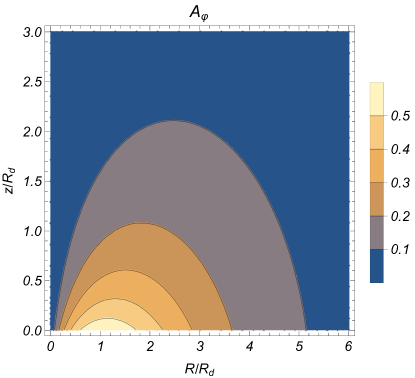
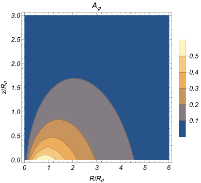
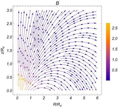
Figure 1.— Top panels: the $A_{\varphi}$ field for the counterclockwise rotating exponential (left) and Kuzmin (right) razor thin disks, in units of $\epsilon\sqrt{GM_{\rm d}/R_{\rm d}}$, where $\epsilon=GM_{\rm d}/(R_{\rm d}c^{2})$. The field is computed for the newtonian current $\chi_{0}$, as required by Equation (21), and it looks similar to the field that would be produced by the current of a circular spire; the maximum of the newtonian current is located at $R_{0}\simeq 0.574R_{\rm d}$ for the exponential disk, and at $R_{0}\simeq 0.535R_{\rm d}$ for the Kuzmin disk. The maximum of $A_{\varphi}$ is located at $R_{A}\simeq 1.12R_{\rm d}$ for the exponential disk and at $R_{A}\simeq 0.85R_{\rm d}$ for the Kuzmin disk. Bottom panels: the corresponding ${\bf B}$ field, in units of $\epsilon\sqrt{GM_{\rm d}/R_{\rm d}^{3}}$. At $z=0$, $B_{z}$ is positive in the inner regions of the disk, and negative outside; the radius $R_{B}$ at which $B_{z}=0$ is determined by the critical point of $RA_{\varphi}(R)$, and so does not coincide with the position of the maximum of $A_{\varphi}(R)$, as apparent from the figures. Numerically, $R_{B}\simeq 2.2R_{\rm d}$ for the exponential disk, and $R_{B}\simeq 1.68$ for the Kuzmin disk.

Figure 2.— The (dimensionless) gravitomagnetic field ${\cal B}$ in the disk plane, for the counterclockwise rotating exponential (solid line), and Kuzmin (dotted line) disks made by purely circular orbits, computed from the newtonian surface current density $\chi_{0}$. $B_{z}$ in the central regions of the disks is positive, i.e. directed along ${\bf e}_{z}$, while in the outer parts $B_{z}$ and ${\bf e}_{z}$ are antiparallel, as also apparent from the bottom panels in Figure 1.

For a razor-thin disk of total mass $M_{\rm d}$ and scale-lenght $R_{\rm d}$, it is natural to normalize lenghts to $R_{\rm d}$, surface densities to $M_{\rm d}/R_{\rm d}^{2}$, and velocities to $\sqrt{GM_{\rm d}/R_{\rm d}}$: a tilde over a quantity indicates normalization to its associated scale. Accordingly, Equation (17) is recast in dimensionless form as

$${\tilde{v}}^{2}={\tilde{v}}_{0}^{2}+\epsilon\,\tilde{R}\,\tilde{v}\,{\cal B}[\tilde{\chi}],\qquad\epsilon={GM_{\rm d}\over R_{\rm d}c^{2}},$$ (19)

where $\epsilon$ is a dimensionless parameter arising naturally from the normalization of ${\bf B}$. In fact, from Equation (18) we obtain $B_{z}=\epsilon\sqrt{GM_{\rm d}/R_{\rm d}^{3}}{\cal B}$, where ${\cal B}$ is the dimensionless gravitomagnetic field in the disk. Notice that for a disk the parameter $\epsilon$ is nothing else that the natural proxy for the quantity $v^{2}/c^{2}$ mentioned in the Introduction, where $v$ is a charaterstic velocity associated to the newtonian gravitational field (see the solid lines in Figure 3). Therefore, in real galaxies $\epsilon$ is very small: for example $\epsilon\simeq 10^{-6}$, in a disk galaxy with a characteristic rotational velocity of $300$ km/s. Accordingly, we represent $v$ as a regular asymptotic series in powers of $\epsilon$

$$v(\epsilon,R)=v_{0}(R)+\epsilon^{\alpha}v_{1}(R)+{\cal O}(\epsilon^{2\alpha}),\qquad\alpha>0,$$ (20)

where the exponent $\alpha$ is to be fixed by order balance, and of course for $\epsilon\to 0$ we reobtain the newtonian case. Inserting the expansion above in Equation (17), from the linearity of $B_{z}[\chi]$ on velocity, it follows necessarily that $\alpha=1$, and at points where ${\tilde{v}}_{0}\neq 0$

$${\tilde{v}}_{1}={\tilde{R}\over 2}{\cal B}[{\tilde{\chi}}_{0}],$$ (21)

where ${\tilde{\chi}}_{0}$ is the (normalized) surface density current profile corresponding to the newtonian rotation curve ${\tilde{v}}_{0}$: from ${\cal O}(B_{z}[\tilde{\chi}_{0}])=\epsilon$, it follows that the term ${\tilde{v}}_{1}$ depends on the gravitomagnetic field produced by the newtonian current only. At the origin, the only point at finite $R$ where ${\tilde{v}}_{0}$ can vanish, the perturbation analysis shows that again $\alpha=1$, but ${\tilde{v}}_{1}=\tilde{R}{\cal B}[{\tilde{\chi}}_{0}]$: however, as $R=0$, no difference arises with Equation (21), that therefore can be used uniformly over the whole radial range. Moreover, Equation (21) shows that the GR corrections due to a counterclockwise current lead to a decrease of the rotational speed where $B_{z}[\chi_{0}]$ is negative, and an increase where $B_{z}[\chi_{0}]$ is positive: of course, it is immediate to verify that the effects on the circular speed are the same for a global inversion of the rotational velocity $v_{0}\to-v_{0}$, due to the associated change of sign of $B_{z}[\chi_{0}]$. It is important to remark that Equation (21) allows for an alternative interpretation: one could just consider the field $B_{z}[\tilde{\chi}_{0}]$ at the r.h.s of Equation (17), and then solve in closed form the resulting quadratic equation for $v(R)$. After selecting the sign so that for $\epsilon\to 0$ the newtonian profile is reobtained, an expansion of the solution for $\epsilon\to 0$, and truncation at the first order, gives again Equation (21), proving again the the linear gravitomagnetic formulation of the problem leads to a regular perturbation problem (e.g., see Bender and Orszag 1978, Chapter 7).

Of course, even if the problem admits a regular perturbation approach, with a solution reducing to the newtonian one in the limit $\epsilon=0$, the function ${\tilde{v}}_{1}$ could attain very large (but finite) values, compensating the small (but non-zero) value of $\epsilon$, and producing a perturbation of the same order of magnitude or even larger than the newtonian term: this would be a strong support to the possibility of a GR origin of the flat rotation curve of disk galaxies. In the next examples, based on realistic disk density profiles, we show however that this is not the case, and ${\tilde{v}}_{1}$ remains small, with absolute values well below the unity.

3.1. The exponential disk

In our first application we consider the razor-thin exponential disk of total mass $M_{\rm d}$ and scale-lenght $R_{\rm d}$, the standard model used to describe the stellar density distribution of disk galaxies (e.g., BT08, Bertin 2014). The surface density is given by

$$\Sigma(R)={M_{\rm d}\over R_{\rm d}^{2}}{{\rm e}^{-\tilde{R}}\over 2\pi},\qquad\tilde{R}={R\over R_{\rm d}},$$ (22)

and in newtonian gravity the gravitational potential in the equatorial plane is

$$\phi(R)=-{GM_{\rm d}\over R_{\rm d}}{\tilde{R}\over 2}\left[{\rm I}_{0}\left({\tilde{R}\over 2}\right){\rm K}_{1}\left({\tilde{R}\over 2}\right)-{\rm I}_{1}\left({\tilde{R}\over 2}\right){\rm K}_{0}\left({\tilde{R}\over 2}\right)\right],$$ (23)

so that the associated circular velocity is

$$v_{0}^{2}(R)={GM_{\rm d}\over R_{\rm d}}{\tilde{R}^{2}\over 2}\left[{\rm I}_{0}\left({\tilde{R}\over 2}\right){\rm K}_{0}\left({\tilde{R}\over 2}\right)-{\rm I}_{1}\left({\tilde{R}\over 2}\right){\rm K}_{1}\left({\tilde{R}\over 2}\right)\right],$$ (24)

where ${\rm I}_{m}$ and ${\rm K}_{m}$ are the modified Bessel functions of order $m$ (e.g., BT08, C21). As already remarked in the Introduction, the maximum of $v_{0}$ is reached at $R\simeq 2.15R_{\rm d}$, and in the range $1.5<\tilde{R}<3$ the curve is almost flat even in absence of DM: notice that inside $3R_{\rm d}$ the disk already contains $\simeq 0.8M_{\rm d}$. The newtonian current surface density $\chi_{0}$ for a disk made by purely circular orbits is then obtained from Equations (22)-(24): for a global counterclockwise rotation, it reaches the maximum at $R_{0}\simeq 0.574R_{\rm d}$.

For the exponential disk it turns out that the most efficient way to compute the gravitomagnetic field is to use the formulation in terms of elliptic integrals. In particular, as the current density is a regular function of $R$, the general discussion about convergence leads to use Equation (11) for the evaluation of $A_{\varphi}$, and the first and second integrals in Equation (12) for the evaluation of $B_{R}$ and $B_{z}$, respectively: of course, in the disk plane the latter expression reduces to the first case in Equation (18). Numerically, the integrable divergence at $\xi=R$ is easily treated by splitting the integral from the origin to $(1-\eta)R$, and from $(1+\eta)R$ to infinity, and reducing $\eta$ until acceptable convergence is reached (actually, thanks to absolute convergence, the two $\eta$’s not need to be the same). In the following experiment, convergence was already reached for $\eta=10^{-3}$, with stable results at 5 significative digits according to Mathematica NIntegrate function. Importantly, the numerical agreement with the alternative formulation in terms of Bessel functions has been also verified over all the disk.

In the top left panel of Figure 1, the only nonvanishing component $A_{\varphi}$ of the potential vector (in units of $\epsilon\sqrt{GM_{\rm d}/R_{\rm d}}$), is shown in the meridional plane, where the overall striking similarity with the field produced by an “effective” circular current loop of radius $R_{A}\simeq 1.12R_{\rm d}$ is apparent, where $R_{A}$ is the position of the maximum of $A_{\varphi}(R)$; quite obviously, $R_{A}$ does not coincide with the position $R_{0}$ of the maximum of the current. In the bottom left panel, the associated (normalized) ${\bf B}$ field is shown. As expected, the field is similar to that of a circular (counterclockwise circulating) current loop, with $B_{z}$ positively directed in the inner regions of the disk (where the Biot-Savart fields of each current ring composing $\chi_{0}$ reinforces), and negatively directed in the outer regions, due to the cooperative (negative) contribution of the current in the inner regions of the disk, while the counteracting positive contributions of the current in the outer regions of the disk are less and less important, due to vanishing of the current at large radii. The radial trend of $B_{z}[\chi_{0}]$ in the disk plane is represented by the solid line in Figure 2. Notice that the radius at which $B_{z}(R)=0$ is $R_{B}\simeq 2.2R_{\rm d}$, not coincident with $R_{A}$, as from Equation (10) $R_{B}$ is given by the critical point of $RA_{\varphi}(R)$, while $R_{A}$ is the critical point of $A_{\varphi}(R)$. Having determined the field $B_{z}$for the exponential disk, from Equation (21) we finally compute $v_{1}$. In the left panel panel of Figure 3 the solid line shows the (normalized) profile of the newtonian rotation curve $v_{0}$, while the dotted line $v_{1}$. After multiplication by $\epsilon\simeq 10^{-6}$, it is clear the the effects of GR on the curve of the exponential disk are well below the possibility of any practical detection, with differences with respect to the newtonian rotation curve well below 1 m/s: at the description level of gravitomagnetism, GR does not produce any effect on the rotation curve of the disk. In any case, it is interesting to notice that for the reasons explained above, the sign of the gravitomagnetic field in the Lorentz equation actually produces a decrease of the rotational speed at large galactocentric distances!

Figure 3.— Radial trend of the rotational velocity components in Equation (20) normalized to $\sqrt{GM_{\rm d}/R_{\rm d}}$, for the exponential (left) and Kuzmin-Toomre (right) disks. The solid line is the newtonian rotation curve $v_{0}$, and the dotted line is the $v_{1}$ perturbative term, that should then be added to $v_{0}$ after multiplication by $\epsilon\simeq 10^{-6}$. Notice how, in principle, the effect of the GR gravitomagnetic field at large radii is a decrease of the circular velocity with respect to the newtonian case.

3.2. The Kuzmin-Toomre disk

Having determined the solution for the exponential disk, in order to confirm the obtained results we move to explore a different disk model. We focus on the Kuzmin-Toomre razor-thin disk (Kuzmin 1956, Toomre 1963, see also BT08, C21), an idealized model widely used stellar dynamics for its mathematical simplicity. The surface density-potential pair of the disk of total mass $M_{\rm d}$ and scale-lenght $R_{\rm d}$ is given by

$$\Sigma(R)={M_{\rm d}\over R_{\rm d}^{2}}{1\over 2\pi(\tilde{R}^{2}+1)^{3/2}},\qquad\phi(R)=-{GM_{\rm d}\over R_{\rm d}}{1\over\sqrt{\tilde{R}^{2}+1}},\qquad\tilde{R}={R\over R_{\rm d}},$$ (25)

where the potential is restricted to the disk plane, and the newtonian circular velocity and the surface mass density current are given by

$$v_{0}^{2}(R)={GM_{\rm d}\over R_{\rm d}}{\tilde{R}^{2}\over(\tilde{R}^{2}+1)^{3/2}},\qquad\chi_{0}(R)=\sqrt{GM_{\rm d}^{3}\over R_{\rm d}^{5}}{\tilde{R}\over 2\pi(\tilde{R}^{2}+1)^{9/4}}.$$ (26)

The maximum of $v_{0}$ is located at $R=\sqrt{2}R_{\rm d}$, and that of $\chi_{0}$ at $R_{0}=\sqrt{2/7}R_{\rm d}\simeq 0.535R_{\rm d}$, a value curiously similar to that of the exponential disk. We now show that $v_{1}$ can be obtained in closed form by using the Fourier-Bessel identity in Equation (18). In fact, from eq. (6.565.4) of GR07, or eq. (2.12.4.28) of P86, we obtain the Hankel transform of order 1 for the newtonian mass current as

$${\hat{\chi}_{1}}(\tilde{\lambda})=\sqrt{GM_{\rm d}^{3}\over R_{\rm d}}\,{{\tilde{\lambda}}^{5/4}{\rm K}_{1/4}(\tilde{\lambda})\over 2^{9/4}\pi\Gamma(9/4)},\qquad\tilde{\lambda}=\lambda R_{\rm d},$$ (27)

where $\Gamma$ is the complete gamma function, and we used the fact that for modified Bessel functions ${\rm K}_{-\nu}={\rm K}_{\nu}$; notice that $\tilde{\lambda}$ is a dimensionless quantity. The last integral in Equation (18) can be expressed analytically thanks to eq. (6.576.3) of GR07 or eq. (2.16.21.1) of P86, and finally from Equation (21) we obtain

$$v_{1}(R)=\sqrt{GM_{\rm d}\over R_{\rm d}}\,{2\Gamma(7/4)\Gamma(3/2)\over\Gamma(9/4)}{{}_{2}F_{1}}\left({7\over 4},{3\over 2};1;-\tilde{R}^{2}\right)\,\tilde{R},$$ (28)

where ${}_{2}F_{1}$ is the standard hypergeometric function. Notice that equation above can be recast in terms of elliptic integrals, resulting in perfect agreement over the whole radial range with the values of $v_{1}(R)$ obtained from Equation (21) and numerical integration of the last expression of $B_{z}$ in Equation (12), in a reassuring validity check. As a mathematical curiosity, we also notice that for the newtonian current $\chi_{0}$ of the Kuzmin-Toomre disk, not only the field $B_{z}$ in the disk plane can be obtained explicitely, but also Equations (15) can be solved analytically over all the space by using Fox H function,s after expressing Equation (27) in terms of these functions (e.g., Mathai et al. 2010, and in particular eq. (2.25.3.2) in Prudnikov et al. 1990): the resulting expression is however of no practical use, and so not reported here.

In the right panels of Figure 1 we plot the normalized potential vector of the disk in the meridional plane, and the associated gravitomagnetic field: the maximum of the gravitomagnetic potential vector is reached at $R_{A}\simeq 0.85R_{\rm d}$. The similarity with the case of the exponential disk, and also the range of values spanned by the normalized fields is remarkably similar, even if the radial density profiles of the two disks are quite different, especially at large radii; notice also the similar behavior of $B_{z}$ in Figure 2, with positive values in the inner regions of the disk (i.e., for $R<R_{B}\simeq 1.68$), and negative values outside. In Figure 3 we plot the normalized profiles of $v_{0}$ and $v_{1}$. It is again apparent how $v_{1}$ remains limited over all the radial range, confirming that the contribute to the rotational velocity of the first order perturbative term in the velocity expansion is fully controlled by the smallness of $\epsilon$, and again the expected GR corrections to the newtonian rotational velocity of the galaxy are well below the detection limit, with differences between the newtonian and the gravitomagnetic GR curve well below 1 m/s. Finally, in accordance with the change of sign of $B_{z}$ along the equatorial plane, the gravitomagnetic effects produce a decrease of the rotational speed at large distances from the galaxy center.

Therefore, from the analysis conducted so far, it seems a quite robust conclusion that GR, at the level of the gravitomagnetic weak field approximation, does not affect the rotation curve of self-gravitating barionic disks with realistic density profiles, and made mostly by circular orbits. In the next Section we relax the assumption of a two-dimensional density distribution, and we also consider non-circular orbits for the stars producing the field in the system.

4. The gravitomagnetic Jeans equations

After the discussion of razor-thin disks, we address the problem of the expected effects of GR on the internal dynamics of genuinely tridimensional (collisionless) astronomical systems, such as finite-thickness disk galaxies, or axisymmetric elliptical galaxies. We first rigorously derive the gravitomagnetic modification of the Jeans equations, and then we restrict to stationary axisymmetric systems. As usual, we indicate with ${\bf v}$ the phase-space velocity, so that the density $\rho$ and the streaming velocity field ${\boldsymbol{v}}$ of the system are given by

$$\rho({\bf x})=\int fd^{3}{\bf v},\qquad{\boldsymbol{v}}({\bf x})\equiv\overline{{\bf v}}={1\over\rho({\bf x})}\int f{\bf v}d^{3}{\bf v},$$ (29)

where $f({\bf x},{\bf v},t)$ is the phase-space distribution function (hereafter DF, see BT08, Bertin 2014, C21), and a bar over a quantity indicates its average over the velocity space. In the following we will write ${\bf v}={\rm v}_{i}{\bf e}_{i}={\rm v}_{R}{\bf e}_{R}+{\rm v}_{\varphi}{\bf e}_{\varphi}+{\rm v}_{z}{\bf e}_{z}$, and ${\boldsymbol{v}}=v_{i}{\bf e}_{i}=v_{R}{\bf e}_{R}+v_{\varphi}{\bf e}_{\varphi}+v_{z}{\bf e}_{z}$, where sums over repeated indices hold in Cartesian coordinates.

Suppose the considered stellar system is self-consistent, i.e., the motion of each star is determined by the field produced by the combined effects of all the other stars. As we are in the low velocity limit, when the Biot-Savart law can be interpreted as the sum of the Lorentz fields produced by each moving charge (an interpretation in general not true for currents produced by particles of arbitrary large velocities, see e.g. J98, Chapter 5; Griffiths 1999, Chapter 5; Feynman 1977, Chapters 13 and 21; Panofsky and Phillips 1962, Chapter 7), it follows that the acceleration experienced by a star at ${\bf x}$ with velocity ${\bf v}$ can be written by summing the r.h.s. member of Equation (2) over the DF,

$${d^{2}{\bf x}\over dt^{2}}=-\nabla\phi-{\bf v}\wedge{\bf B}[{\bf j}],\qquad{\bf j}({\bf x})=\rho{\boldsymbol{v}}=\int f{\bf v}d^{3}{\bf v},$$ (30)

where $\phi({\bf x})$ is the newtonian gravitational potential of the system and ${\bf B}[{\bf j}]$, by virtue of the linearity of ${\bf B}$ on the current, is the gravitomagnetic field produced at ${\bf x}$ by the total streaming current of the system. The hierarchy of the Jeans equations of increasing order is then obtained by taking moments over the velocity space of the collisionless Boltzamnn equation (e.g., see BT08, C21)

$${\partial f\over\partial t}+{\rm v}_{i}{\partial f\over\partial x_{i}}+{d{\rm v}_{i}\over dt}{\partial f\over\partial{\rm v}_{i}}=0,$$ (31)

here written in Cartesian coordinates. After multiplication of Equation (31) by $1$, ${\rm v}_{i}$, ${\rm v}_{i}{\rm v}_{j}$, etc., and integration, the three second order moments equations (the gravitomagnetic modification of the usual Jeans equations of stellar dynamics) are given by

$${\partial\rho v_{i}\over\partial t}+{\partial\rho\overline{{\rm v}_{i}{\rm v}_{k}}\over\partial x_{k}}=-\rho{\partial\phi\over\partial x_{i}}-\epsilon_{ijk}\rho v_{j}B_{k}[{\bf j}],\qquad i=1,2,3,$$ (32)

where

$$\overline{{\rm v}_{i}{\rm v}_{j}}({\bf x})={1\over\rho({\bf x})}\int f\,{\rm v}_{i}{\rm v}_{j}d^{3}{\bf v},\qquad\sigma^{2}_{ij}({\bf x})=\overline{({\rm v}_{i}-v_{i})({\rm v}_{j}-v_{j})}=\overline{{\rm v}_{i}{\rm v}_{j}}-v_{i}v_{j};$$ (33)

in particular, $\sigma_{ij}^{2}$ are the components of the second-order velocity dispersion tensor. In Appendix B, the general gravitomagnetic time-dependent Jeans equations are also reported in cylindrical coordinates.

We now to restrict to the axysimmetric stationary case. In the usual stellar dynamical case, from the Jeans theorem one would assume a phase-space DF depending on the two classical integrals of the motion (per unit mass) $E$ and $J_{z}$, i.e. the orbital energy, and the $z$-component of the angular momentum of stellar orbits. As well known, under this assumption (e.g., BT08, C21), important constraints on the allowed velocity moments follow, namely 1) the only possible streaming motions are in the azimuthal direction, i.e., ${\boldsymbol{v}}=v_{\varphi}(R,z){\bf e}_{\varphi}$, and 2) the velocity dispersion tensor is in diagonal form at each point in the system, with $\sigma_{R}^{2}=\sigma_{z}^{2}\equiv\sigma^{2}$, while only $\overline{v_{\varphi}^{2}}=\sigma_{\varphi}^{2}+v_{\varphi}^{2}$ remains determined; when $\sigma_{\varphi}^{2}=\sigma^{2}$ everywhere, the system is said isotropic. Therefore, for stationary stellar dynamical two-integral axisymmetric systems with $f(E,J_{z})$, the current would be of the “circular type” considered in Equation (7), with ${\bf j}=j{\bf e}_{\varphi}=\rho v_{\varphi}{\bf e}_{\varphi}$: notice that, even if the current associated with the streaming velocity field is circular, the orbits of the individual stars contributing to the resulting gravitomagnetic field are in general not circular, and so we are considering an orbital structure more complicated than that of the razor-thin disk in Section 3.

However, in the case of stationary collisionless stellar systems with gravitomagnetic forces, the situation is not so simple, because while $E$ is still an integral of motion, $J_{z}$ is not conserved along orbits and so it cannot be used as an isolating integral in the DF. Fortunately, the problem is solved as follows. As well known, the lagrangian (per unit mass) associated with Equation (30) is

$${\cal L}={\|{\bf v}\|^{2}\over 2}-(\phi+{\bf A}\cdot{\bf v}),$$ (34)

where at variance with the EM case (e.g., see Landau and Lifshitz 1971) the + sign in the generalized potential derives from the - sign in the gravitomagnetic Lorentz force. Suppose now that ${\boldsymbol{v}}=v_{\varphi}(R,z){\bf e}_{\varphi}$, so that ${\bf A}=A_{\varphi}(R,z){\bf e}_{\varphi}$ from the results in Section 2.1. The Euler-Lagrange equations show immediately that $J_{z}$ is not conserved, but a second integral of motion exists, $I_{2}=J_{z}-RA_{\varphi}$. The Jeans theorem then in principle allows for a two-integrals DF $f(E,I_{2})$, and the interesting question arises wether such a DF is consistent with the assumption of streaming motions with ${\boldsymbol{v}}=v_{\varphi}(R,z){\bf e}_{\varphi}$ used to prove the existence of $I_{2}$. The answer is in the affirmative, and it is easy to prove that the properties (1) and (2) mentioned above for systems supported by a $f(E,J_{z})$ are preserved by the generalized $f(E,I_{2})$, in particular the fact that $v_{R}=v_{z}=0$. Therefore, the vertical and radial Jeans equations (B2) for a stationary, axisymmetric two-integrals system with gravitomagnetic forces, supported by a DF of the family $f(E,I_{2})$, become

$$\begin{cases}\displaystyle{{\partial\rho\sigma^{2}\over\partial z}=-\rho{\partial\phi\over\partial z}+jB_{R}[j],\qquad j=\rho v_{\varphi},}\cr\cr\displaystyle{{\partial\rho\sigma^{2}\over\partial R}-{\rho\Delta\over R}=-\rho{\partial\phi\over\partial R}-jB_{z}[j],}\end{cases}$$ (35)

where $\Delta=\overline{{\rm v}_{\varphi}^{2}}-\sigma^{2}$, and in the isotropic rotator case $\Delta=v_{\varphi}^{2}$. Finally, the azimuthal Jeans equation vanishes identically also in the gravitomagnetic case, as obvious from the last of Equations (B2). Notice how at variance with the classical newtonian case, now the vertical and radial velocity dispersions depend on the ordered rotational field $v_{\varphi}(R,z)$, yet to be determined.

Equations (35) can be formally solved in terms of $\sigma^{2}$ and $\Delta$ as in the usual stellar dynamical case, obtaining

$$\rho\sigma^{2}=\int_{z}^{\infty}\rho{\partial\phi\over\partial z^{\prime}}\,dz^{\prime}-U=\rho\sigma_{0}^{2}-U,\qquad U(R,z)=\int_{z}^{\infty}jB_{R}[j]\,dz^{\prime},$$ (36)

where $\sigma_{0}^{2}$ is the newtonian solution, and $U(R,z)$ accounts for the gravitomagnetic effects. Moreover, some algebra shows that

$${\rho\Delta\over R}=C[\rho,\phi]-V,\qquad C[\rho,\phi]=\int_{z}^{\infty}\left({\partial\rho\over\partial R}{\partial\phi\over\partial z^{\prime}}-{\partial\rho\over\partial z^{\prime}}{\partial\phi\over\partial R}\right)\,dz^{\prime}={\rho\Delta_{0}\over R}$$ (37)

where the commutator $C[\rho,\phi]$ is the standard newtonian solution (e.g., Hunter 1977, Barnabè et al. 2006, see also C21), while the term

$$V(R,z) = \int_{z}^{\infty}\left({\partial jB_{R}\over\partial R}+{\partial jB_{z}\over\partial z^{\prime}}\right)\,dz^{\prime}=\int_{z}^{\infty}\left[\left({\partial\over\partial R}{j\over R}\right)RB_{R}+{\partial j\over\partial z^{\prime}}B_{z}\right]\,dz^{\prime}$$ (38)

$$= -C[j,A_{\varphi}]-{jA_{\varphi}\over R},$$ (39)

contains the gravitomagnetic effects. The triple integral in the second expression above (obtained from the first by exploiting the solenoidal nature of ${\bf B}$) is particularly well suited for numerical computations when the current is analitically available (see next Section), while the last expression is obtained from the first taking into account that ${\bf B}=\nabla\wedge{\bf A}$, Equation (10), and finally integrating by parts with $jA_{\varphi}=0$ for $z\to\infty$.

As noticed, the difficulty in the solution of the gravitomagnetic Jeans equations is the fact that the force field depends on the azimuthal streaming velocity distribution, a quantity that it is not known in advance. In principle, to solve the gravitomagnetic Jeans equations one should 1) impose a decomposition on the still unknown azimuthal velocity field, for example by using the widely adopted Satoh (1980) ansatz $v_{\varphi}^{2}=k^{2}\Delta$ (e.g., see C21), 2) solve the resulting nonlinear integrodifferential Equation (37) for $v_{\varphi}$ and obtain $B_{R}[j]$, 3) integrate Equation (36) and obtain $\sigma^{2}$, 4) conclude by determining $\Delta$ and the tangential velocity dispersion $\sigma_{\varphi}^{2}=\sigma^{2}+(1-k^{2})\Delta=\sigma^{2}+(1/k^{2}-1)v_{\varphi}^{2}$. Quite obviously, a considerable simplification is achieved by exploiting the fact that in Equation (35) the fields $B_{R}$ and $B_{z}$ are proportional to the small parameter $\epsilon=GM_{*}/(r_{*}c^{2})$, where $M_{*}$ is the total mass of the system, and $r_{*}$ its scale-lenght. As in the razor-thin disks, it follows immediately that the first order perturbative terms in the natural expansions $\sigma^{2}=\sigma_{0}^{2}+\epsilon\sigma_{1}^{2}\ldots\;$, $\Delta=\Delta_{0}+\epsilon\Delta_{1}\ldots\;$, and $v_{\varphi}=v_{\varphi 0}+\epsilon v_{\varphi 1}\ldots\;$, are related to the functions $U$ and $V$ evaluated over the newtonian current $j_{0}=\rho v_{\varphi 0}$, where $v_{\varphi 0}(R,z)$ is the streaming rotation velocity obtained from the classical Jeans equations.

We are now in position to evaluate the effects of GR corrections on the circular velocity $v(\epsilon,R)=v_{0}(R)+\epsilon v_{1}(R)+\ldots\;$ of a test star in the equatorial plane of an axisymmetric collisionless system described by Equations (35). The only difference with the razor-thin disks in Section 3 is that now the current is provided by the azimuthal streaming velocity field of the system. From Equation (30), the analogous of Equations (17) and (19) still apply, and

$${\tilde{v}}_{1}={\tilde{R}\over 2}{\cal B}[{\tilde{\j}}_{0}],$$ (40)

$B_{z}=\epsilon\sqrt{GM_{*}/r_{*}^{3}}{\cal B}$ is computed in the disk plane, and finally $j_{0}=\sqrt{GM_{*}^{3}/r_{*}^{7}}\,{\tilde{\j}}_{0}$.

The expression for the first order correction term to the streaming velocity (restricting for simplicity to the isotropic rotator case for the stellar distribution of the galaxy) is instead obtained from Equation (37), considering that at the lowest order $V={\cal O}(\epsilon)$, and so from $v_{\varphi}=v_{\varphi 0}+\epsilon v_{\varphi 1}\ldots\;$, after order balance and some simplification, one gets

$$\tilde{v}_{\varphi 1}=-{\tilde{R}\over 2\tilde{\j}_{0}}{\cal V}[{\tilde{\j}}_{0}],$$ (41)

where $V=\epsilon(GM_{*}^{2}/r_{*}^{5}){\cal V}$ is computed from Equation (39).

4.1. The Miyamoto-Nagai disk

We now solve the gravitomagnetic Jeans equations, and evaluate Equations (40)-(40) for the widely used Miyamoto-Nagai (1975, Nagai and Miyamoto 1976, see also BT08, C21) disk of total mass $M_{*}$ and scale-lengths $a$ and $b$, with newtonian density-potential pair

$$\rho(R,z)={M_{*}\over a^{3}}{s^{2}\over 4\pi}{\tilde{R}^{2}+(1+3\zeta)(1+\zeta)^{2}\over\zeta^{3}\,[\tilde{R}^{2}+(1+\zeta)^{2}]^{5/2}},\qquad\phi(R,z)=-{GM_{*}\over a}{1\over\sqrt{\tilde{R}^{2}+(1+\zeta)^{2}}},$$ (42)

where $\zeta=\sqrt{\tilde{z}^{2}+s^{2}}$, $\tilde{R}=R/a$, $\tilde{z}=z/a$, and the newtonian circular velocity in the equatorial plane is given by

$$v_{0}^{2}(R)={GM_{*}\over a}{\tilde{R}^{2}\over[\tilde{R}^{2}+(1+s)^{2}]^{3/2}}.$$ (43)

the dimensionless parameter $s=b/a$ measures the disk flattening, and for $b=0$ the model reduces to the Kuzmin disk of total mass $M_{*}$ and scale-lenght $a$, so we are in the condition to explore the GR effects of a non-zero thickness on the rotation curve, by comparison with the case in Section 3.2.

We restrict for simplicity to the isotropic rotator, with a conterclockwise streaming velocity field, so that the newtonian azimuthal streaming velocity field and the associated current density are

$$\begin{cases}\displaystyle{v_{\varphi 0}^{2}(R,z)={GM_{*}\over a}{\tilde{R}^{2}\over[\tilde{R}^{2}+(1+3\zeta)(1+\zeta)^{2}]\sqrt{\tilde{R}^{2}+(1+\zeta)^{2}}},}\cr\cr\displaystyle{j_{0}(R,z)=\sqrt{{GM_{*}^{3}\over a^{7}}}{s^{2}\over 4\pi}{\tilde{R}\sqrt{\tilde{R}^{2}+(1+3\zeta)(1+\zeta)^{2}}\over\zeta^{3}[\tilde{R}^{2}+(1+\zeta)^{2}]^{11/4}},}\end{cases}$$ (44)

(e.g., Ciotti and Pellegrini 1996, Smet et al. 2015). Notice that in the equatorial plane the location of the maximum of $j_{0}(R,0)$ can be evaluated analytically as a biquadratic equation, and for $s\to 0$ the position coincides with that of the maximum for the Kuzmin disk.

In the left panel of Figure 4 we show the results for the circular velocity, to be compared with the analogous Figure 3 for the two razor thin disks made by circular orbits. The solid line represents the newtonian circular velocity $\tilde{v}_{0}$ in Equation (43), while the dotted line gives the correction term in Equation (40), where the gravitomagnetic field is now produced by stars that in general are not moving in circular orbits. Again, for realistic mass distributions, the perturbation term shoud be multiplied by factor $\epsilon\approx 10^{-6}$ before addition to the newtonian term: the GR effects appear again to be completely negligible and, in analogy with the case of razor thin disks, positive in the inner regions of the galaxy, and negative at large radii, reducing there the rotational speed of a test mass. In the right panel we show instead the streaming velocity of stars in the disk equatorial plane, both the newtonian component (solid line), and the lowest order GR term (dotted line). Again, it is important to remark that the orbits of the individual stars producing the $v_{\varphi}$ in the equatorial plane are in general not circular, and not restricted to the equatorial plane. Notice how the newtonian streaming velocity is slightly below the newtonian circular velocity, the well known phenomenon of asymmetric drift, due to effect of the vertical component of the velocity dispersion tensor: (e.g., see BT08). Notice also how the asymmetric drift (a small but well measured phenomenon in real galaxies) is several order of magnitude larger than the GR corrections.

The results for the Miyamoto-Nagai disk reinforces the previous conclusions, i.e., also in three dimensional galaxies, with stars moving on non-circular orbits, the GR effects predicted by linear gravitomagnetism on the rotational velocities are a factor of $\approx 10^{-6}$ smaller than the newtonian predictions. If newtonian gravity requires DM, unless “strong” weak-field GR effects (beyond the linear gravitomagnetic description) actually dominates the dynamics of the galaxies, exactly the same amount and distribution of DM is required in GR and in newtonian gravity, in order to reproduce the observed rotational curves.

Figure 4.— Radial trend of the rotational velocity components (left), and of the streaming velocity (right), normalized to $\sqrt{GM_{*}/a}$, in the equatorial plane of the counterclockwise rotating isotropic Miyamoto-Nagai disk with flattening parameter $s=b/a=0.1$. The solid lines are the newtonian components, and the dotted lines are the first perturbative term, that should be added to the corresponding newtonian term after multiplication by $\epsilon\simeq 10^{-6}$. Note how the circular velocity is slightly larger than the streaming velocity, the well known phenomenon of asymmetric drift produced by the disk vertical velocity dispersion support.

5. Discussion and conclusions

Recently, it has been suggested that the observed flat radial profile of the rotation curves of disk galaxies at large galactocentric radii could be a peculiar effect of GR in rotating systems, instead of the dynamical signature of the presence of DM halos. The suggestion is somewhat puzzling, as observed galaxies are empirically in a weak-field regime, with $v/c\approx 10^{-3}$, and so GR corrections are expected to be very small: however, GR is a non-linear theory, and so important effects cannot be excluded in principle.

In this paper, instead of attempting a GR modelization of the rotation curve of some observed galaxy, we followed a different approach, and we built the rotation curve for purely barionic disks, structurally resembling real galaxies, and with total mass and scale lenght in the observed range. The rotation curves are computed both in newtonian gravity and in the (gravitomagnetic) weak field formulation of GR, and compared. After a detailed discussion of the mathematics, we considered first the case of razor-thin disks made by purely circular orbits. The orbital structure is highly idealized, but the surface density of the disk is the standard exponential profile adopted to model the stellar distribution in real disk galaxies; we also considered another disk model, the Kuzmin-Toomre model, to gain confidence with the results obtained for the exponential disk. Consistently with the gravitomagnetic approximation adopted, we impose “self-consistency” on the rotational velocity, i.e., we assume that the rotational velocity of the test particle (star, or gas cloud), and the rotational velocity of the stellar population producing the gravitomagnetic field, are the same at each radius, and we require that the rotational velocity is the solution of the Lorentz-like equation of motion. The resulting problem is shown to be a regular perturbation problem, with an intrinsinc order parameter $\epsilon\approx 10^{-6}$, and the gravitomagnetic field is obtained from two different (but equivalent) methods, i.e., by using elliptic integrals and Bessel functions. It is found that the GR (normalized) perturbative term is of the order of the unity, with no indications of anomalously large emerging effects, and the resulting physical modification of the newtonian rotation curve is therefore of the order of $\epsilon\approx 10^{-6}$, well below the possibility to detection in observed rotation curves, in agreement with the order-of-magnitude estimate obtained by Toth (2021). Curiously, in the external regions of the disk the gravitomagnetic GR perturbative term tend to decrease the rotational speed, as can be easily understood by considering the gravitomagnetic field as given by the sum of the fields produced by each current ring of the disk, and by the fact that the disk current in realistic disk galaxies decreases sufficiently fast at increasing radius, so that in the outer regions of the disk the gravitomagnetic field is dominated by the inner current distribution. An important warning follows: if one assumes a disk surface density distribution with a sufficiently slow radial decline at increasing $R$, it is quite easy to show that the sum of the fields of external rings can be very large (or even diverge) leading to the wrong conclusion of a significant GR effect in real galaxies: in theoretical/numerical studies of the present problem, the use of realistic density profiles for the disks it is of fundamental importance.

As doubts have been casted that disk thickness effects, or motions more complicated than purely circular orbits for the stars producing the gravitomagnetic fields, could be important, we also studied the case of the gravitomagnetic rotation curve in genuinely tridimensional stellar systmes. We first derived the gravitomagnetic Jeans equations starting directly form the collisionless Boltzamnn equation, and the associated Jeans theorem. In this case the equations contain naturally a vertical “pressure” term due to the vertical velocity dispersion. We showed how in axisymmetric systems the gravitomagnetic field depends on the azimuthal streaming velocity field of the system (even though the orbits of the single stars are in general not axisymmetric). In such a system, we can identity two different rotational velocities: the circular velocity of a tracer in the equatiorial plane, and the (circular) streaming velocity of the stellar population producing the gravitomagnetic field. For both cases we found that the GR perturbative term, after multiplication by the expansion parameter $\epsilon\approx 10^{-6}$, is completely negligible over the newtonian term, so that also for collisionless axysimmetric systems the GR effects due to rotation appear to be well below detectability, and unable to reproduce a flat rotation curve at large radii any better than a newtonian model in absence of DM.

In conclusion, the study conducted in the paper excludes the possibility that gravitomagnetic GR effects can compensate by any detectable amount the keplerian fall of the rotational velocity that would characterize disk galaxies at large distances in absence of DM halos, and produce the observed flat profiles: from the observational point of view, in rotating disk galaxies DM is required by GR exactly as in newtonian gravity. Of course, if a full GR simulation for the same barionic disks used in this papers (with disk parameters corresponding to the observed weak field regime of real galaxies) convincingly proves the opposite, then among other things we should conclude that gravitomagnetic weak field approximation of GR cannot be used to describe the weak field regime in rotating galactic disks.

Appendix A Mathematical identities

Here we list the most important mathematical identities used in this work (see, e.g., BT08, C21, J98), and references therein).

The rotor of a vector function in cyclindrical coordinates is given by

$$\nabla\wedge{\bf A}=\left({1\over R}{\partial A_{z}\over\partial\varphi}-{\partial A_{\varphi}\over\partial z}\right){\bf e}_{R}+\left({\partial A_{R}\over\partial z}-{\partial A_{z}\over\partial R}\right){\bf e}_{\varphi}+{1\over R}\left({\partial RA_{\varphi}\over\partial R}-{\partial A_{R}\over\partial\varphi}\right){\bf e}_{z}.$$ (A1)

The complete elliptic integrals of first and second kind in Legendre form are given respectively by

$$\begin{cases}\displaystyle{{\bf K}(k)=\int_{0}^{\pi/2}{d\varphi^{\prime}\over\sqrt{1-k^{2}\sin^{2}\varphi^{\prime}}}=\int_{0}^{1}{dt\over\sqrt{(1-t^{2})(1-k^{2}t^{2})}},}\cr\cr\displaystyle{{\bf E}(k)=\int_{0}^{\pi/2}\sqrt{1-k^{2}\sin^{2}\varphi^{\prime}}d\varphi^{\prime}=\int_{0}^{1}\sqrt{{1-k^{2}t^{2}\over 1-t^{2}}}dt;}\end{cases}$$ (A2)

and from eq. (8.123) of GR07,

$$\begin{cases}\displaystyle{{d{\bf K}(k)\over dk}={{\bf E}(k)\over k(1-k^{2})}-{{\bf K}(k)\over k},}\cr\cr\displaystyle{{d{\bf E}(k)\over dk}={{\bf E}(k)-{\bf K}(k)\over k}.}\end{cases}$$ (A3)

The two integrals over $\varphi^{\prime}$ in Equations (8)-(9) leading to Equations (11)-(12), after reduction to the first quadrant with the bisection formula $\cos\varphi^{\prime}=2\cos^{2}(\varphi^{\prime}/2)-1$, become

$${\cal F}_{0}=\int_{0}^{2\pi}{d\varphi^{\prime}\over\sqrt{R^{2}+\xi^{2}-2R\xi\cos\varphi^{\prime}+\Delta z^{2}}}={4{\bf K}(k)\over\sqrt{(R+\xi)^{2}+\Delta z^{2}}},$$ (A4)

$${\cal F}_{1}=\int_{0}^{2\pi}{\cos\varphi^{\prime}\,d\varphi^{\prime}\over\sqrt{R^{2}+\xi^{2}-2R\xi\cos\varphi^{\prime}+\Delta z^{2}}}={4\over\sqrt{(R+\xi)^{2}+\Delta z^{2}}}\left[\left({2\over k^{2}}-1\right){\bf K}(k)-{2{\bf E}(k)\over k^{2}}\right],$$ (A5)

where

$$k^{2}={4R\xi\over(R+\xi)^{2}+\Delta z^{2}},\qquad\Delta z=z-z^{\prime}.$$ (A6)

For the considerations in Sections 2.1 and 2.2, we recall the important identity

$$-{\partial{\cal F}_{0}\over\partial\xi}={1\over R}{\partial\,R{\cal F}_{1}\over\partial R},$$ (A7)

that can be proved by differentiation of the explicit expressions in Equations (A4)-(A5), or (with some work) more elegantly directly from their integral representation.

In numerical applications, when using Equations (11)-(12), it is important to recall that ${\bf E}(k)\sim 1$ for $k\to 1^{-}$, but ${\bf K}(k)\sim-\ln\sqrt{1-k^{2}}\sim-\ln\sqrt{1-k}$, so that near the ring $\xi=R$ in the $\Delta z=0$ plane both ${\cal F}_{0}$ and ${\cal F}_{1}$ diverge as

$${\cal F}_{0}\sim{\cal F}_{1}\sim\begin{cases}\displaystyle{-{4\ln|R-\xi|\over R+\xi},\qquad\Delta z=0,\quad\xi\to R;}\cr\cr\displaystyle{-{2\ln|\Delta z|\over R},\qquad\quad\xi=R,\quad\Delta z\to 0};\end{cases}$$ (A8)

however the singularity is integrable and easily treated numerically.

From the theory of Green functions it is possible to prove that in cylindrical coordinates (e.g., BT08, C21)

$${1\over\|{\bf x}-{\bf y}\|}=\sum_{m=-\infty}^{\infty}{\rm e}^{im(\varphi-\varphi^{\prime})}\int_{0}^{\infty}{\rm e}^{-\lambda|\Delta z|}{\rm J}_{m}(\lambda R){\rm J}_{m}(\lambda\xi)\,d\lambda,$$ (A9)

where ${\rm J}_{m}$ are the Bessel functions of first kind and integer order $m$, ${\bf x}=(R\cos\varphi,R\sin\varphi,z)$, ${\bf y}=(\xi\cos\varphi^{\prime},\xi\sin\varphi^{\prime},z^{\prime})$, and the Hankel transform for a function $f(R)$ of the cylindrical radius reads

$${\hat{f}}_{m}(k)=\int_{0}^{\infty}R\,{\rm J}_{m}(\lambda R)\,f(R)\,dR,\qquad f(R)=\int_{0}^{\infty}\lambda\,{\rm J}_{m}(\lambda)\,{\hat{f}}_{m}(\lambda)\,d\lambda.$$ (A10)

Appendix B Gravitomagnetic Jeans equations in cylindrical coordinates

By using the standard approach of considering velocity moments of Equation (31), and by working on cylindrical coordinates, from the velocity moment of order 0 we obtain the continuity equation

$${\partial\rho\over\partial t}+{1\over R}{\partial R\rho v_{R}\over\partial R}+{1\over R}{\partial\rho v_{\varphi}\over\partial\varphi}+{\partial\rho v_{z}\over\partial z}=0,$$ (B1)

and from the three moments of order 1 (respectively over ${\rm v}_{z}$, ${\rm v}_{R}$, and ${\rm v}_{\varphi}$) the three momentum equations

$$\begin{cases}\displaystyle{{\partial\rho v_{z}\over\partial t}+{1\over R}{\partial R\rho\overline{{\rm v}_{R}{\rm v}_{z}}\over\partial R}+{1\over R}{\partial\rho\overline{{\rm v}_{\varphi}{\rm v}_{z}}\over\partial\varphi}+{\partial\rho\overline{{\rm v}_{z}^{2}}\over\partial z}=-\rho{\partial\phi\over\partial z}-\rho(v_{R}B_{\varphi}-v_{\varphi}B_{R}),}\cr\cr\displaystyle{{\partial\rho v_{R}\over\partial t}+{\partial\rho\overline{{\rm v}_{R}^{2}}\over\partial R}-{\rho(\overline{{\rm v}_{\varphi}^{2}}-\overline{{\rm v}_{R}^{2}})\over R}+{1\over R}{\partial\rho\overline{{\rm v}_{R}{\rm v}_{\varphi}}\over\partial\varphi}+{\partial\rho\overline{{\rm v}_{R}{\rm v}_{z}}\over\partial z}=-\rho{\partial\phi\over\partial R}-\rho(v_{\varphi}B_{z}-v_{z}B_{\varphi}),}\cr\cr\displaystyle{{\partial\rho v_{\varphi}\over\partial t}+{1\over R^{2}}{\partial R^{2}\rho\overline{{\rm v}_{R}v_{\varphi}}\over\partial R}+{1\over R}{\partial\rho\overline{{\rm v}_{\varphi}^{2}}\over\partial\varphi}+{\partial\rho\overline{{\rm v}_{\varphi}{\rm v}_{z}}\over\partial z}=-{\rho\over R}{\partial\phi\over\partial\varphi}-\rho(v_{z}B_{R}-v_{R}B_{z}),}\end{cases}$$ (B2)

where the ${\bf B}$ field is determined by Equation (3) computed over the galaxy streaming mass density current given by the second of Equation (30). Finally, if the system is in steady state, and supported by a phase-space DF $f(E,J_{z}-RA_{\varphi})$, from the discussion in Section 4 it follows that Equation (B1) and the last of Equations (B2) are identically verified, while the first two of Equations (B2) reduce to Equation (35).

References

- Astesiano (2022) Astesiano, D., Ruggiero, M.L. 2022, arXiv:2205.03091v1
- Balasin (2008) Balasin, H., Grumiller, D. 2008, Int. J. Mod. Phys. D, 17, 475
- Barnabe‘e (2006) Barnabè, M., Ciotti, L., Fraternali, F., Sancisi, R. 2006, A&A, 446, 61
- Bender (1978) Bender, C.M., Orszag, S. 1978, Advanced Mathematical Methods for Scientists and Engineers, McGraw Hill
- Bertin (2014) Bertin, G., 2014, Dynamics of Galaxies, 2nd ed. Cambridge University Press, Cambridge, UK
- Binney (2008) Binney, J., Tremaine, S. 2008, Galactic Dynamics, 2nd ed. Princeton University Press, Princeton, NJ (BT08)
- Carrick (2012) Carrick, J.D., Cooperstock, F.I. 2012, Astrophys. Space Sci., 337, 321
- Casertano (1983) Casertano, S. 1983, MNRAS, 203, 735
- Ciotti (2021) Ciotti, L. 2021, Introduction to Stellar Dynamics, Cambridge University Press, Cambridge, UK (C21)
- Ciotti (1996) Ciotti, L., Pellegrini, S. 1996, MNRAS, 279, 240
- Clark (2000) Clark, S.J., Tucker, R.W., arXiv:gr-qc/0003115v2
- Cooperstock (2007) Cooperstock, F.I., Tieu, S. 2007, Int. J. Mod. Phys. A, 22, 2293
- Costa (2021) Costa, L.F.O., Natário, J. 2021, arXiv:2109:14641
- Cross (2006) Cross, D.J. 2006, arXiv:astro-ph/0601191v1
- Crosta (2020) Crosta, M., Giammaria, M., Lattanzi, M., Poggio, E. 2020, MNRAS, 496, 2107
- Deledicque (2019) Deledicque, V. 2019, https://hal.archives-ouvertes.fr/hal-01857305v3
- Feynman (1977) Feynman, R.P., Leighton, R.B., Sands, M. 1977, The Feynman Lectures on Physics, volume 2, Addison Wesley
- Fitzpatrick (2012) Fitzpatrick, R. 2012, An Introduction to Celestial Mechanics, Cambridge University Press
- Fuchs (2006) Fuchs, B., Phleps, S. 2006, arXiv:astro-ph/0604022v1
- Gradshteyn (2007) Gradshteyn, I.S., Ryzhik, I.M., Jeffrey, A., Zwillinger, D. 2007, Table of Integrals, Series, and Products, 7th ed. Elsevier (GR07)
- Griffiths (1999) Griffiths, D.J. 1999, Introduction to Electrodynamics, Prenctice Hall
- Hunter (1977) Hunter, C. 1977 AJ, 82, 271
- Jackson (1998) Jackson, D. 1998, Classical Electrodynamics, 3rd ed. John Wiley & Sons (J98)
- Kalnajs (1983) Kalnajs, A. J. 1983 In Internal kinematics of galaxies (IAU symposium no. 100) (ed. E. Athanassoula), p.87. Dordrecht: Reidel
- Kent (1986) Kent, S.M. 1986, AJ, 91, 1301
- Korzynski (2005) Korzynski, M. 2005, arXiv:astro-ph/0508377v2
- Kuzmin (1956) Kuzmin, J.G. 1956, Astron. Zh., 33, 27
- Landau (1971) Landau, L.D., Lifshitz, E.M. 1971, The Classical Theory of Fields, Pergamon Press
- Lynden-Bell (1998) Lynden-Bell, D., Nouri-Zonoz, M. 1998, Rev. of Modern Physics, 70, 427
- Ludwig (2021) Ludwig, G.O. 2021, European Physical Journal C 81, 186
- Ludwig (2022) Ludwig, G.O. 2022, European Physical Journal C 82, 281
- Mashhoon (2008) Mashhoon, B. 2008, arXiv:gr-qc/0311:030
- Mashhoon (1999) Mashhoon, B., Gronwald, F., Lichtenegger, I.M., 1999, arXiv:gr-qc/9912027v1
- Mathai (2010) Mathai, A.M., Saxena, R.K., Haubold, H.J. 2010, The H-Function, Springer
- Miyamoto (1975) Miyamoto, M., Nagai, R. 1975, PASJ, 27, 533
- Nagai (1976) Nagai, R., Miyamoto, M. 1976, PASJ, 28, 1
- Ostriker (1973) Ostriker, J.P., Peebles, P.J.E. 1973, ApJ, 186, 467
- Panofsky (1962) Panofsky, W.K.H, Phillips, M. 1962, Classical Electricity and Magnetism, Second Edition, Addison Wesley
- Poisson (2014) Poisson, E., Will, C.M. 2014, Gravity, Cambridge University Press, UK
- Prudnikov (1986) Prudnikov, A.P., Brychkov, Yu.A., Marichev, O.I. 1986, Integrals and Series, volume 2, Gordon and Breach (P86)
- Prudnikov (1990) Prudnikov, A.P., Brychkov, Yu.A., Marichev, O.I. 1990, Integrals and Series, volume 3, Gordon and Breach
- Rindler (1997) Rindler, W. 1997, Phys. Lett. A, 233, 25
- Ruggiero (2021) Ruggiero, M. L. 2021, Universe, 7, 451
- Ruggiero (2021) Ruggiero, M. L., Ortolan, A., Speake, C.C. 2021, arXiv:2112.08290v1
- Ruggiero (2002) Ruggiero, M. L., Tartaglia, 2002, arXiv:gr-qc/0207065v2
- Satoh (1980) Satoh, C. 1980, PASJ, 32, 41
- Smet (2015) Smet, C.O., Posacki, S., Ciotti, L. 2015, MNRAS, 448, 2921
- Toth (2021) Toth, V.T. 2021, arXiv:2109.00357
- Toomre (1963) Toomre, A. 1963, ApJ, 138, 385
- vanAlbada (1985) van Albada, T.S., Bahcall, J.N., Begeman, K., Sancisi, R. 1985. ApJ, 295, 305
- vanAlbada (1986) van Albada, T.S., Sancisi, R. 1986, Phyl.Trans. R. Soc. Lond. A,320, 447
- Vogt (2005a) Vogt, D., Letelier, P.S. 2005a, arXiv:astro-ph/0510750v1
- Vogt (2005b) Vogt, D., Letelier, P.S. 2005b, arXiv:astro-ph/0512553v1