Quantum critical points, lines and surfaces

Abstract

In this paper we promote the idea of quantum critical lines (inter alia surfaces) as opposed to points. A quantum critical line obtains when criticality at zero temperature is extended over a continuum in a one-dimensional line. We base our ideas on a simple but exactly solved model introduced by one of the authors involving a one-dimensional quantum transverse field Ising model with added 3-spin interaction. While many of the ideas are quite general, there are other aspects that are not. In particular, a line of criticality with continuously varying exponents is not captured. However, the exact solvability of the model gives us considerable confidence in our results. Although the pure system is analytically exactly solved, the disorder case requires numerical analyses based on exact computation of the correlation function in the Pfaffian representation. The disorder case leads to dynamic structure factor as a function of frequency and wave vector. We expect that the model is experientally realizable and perhaps many other similar models will be found to explore quantum critical lines.

I INTRODUCTION

Quantum critical point (QCP)Hertz (1976) is an important widely discussed topic.Continentino (2017); Sachdev (2005) Yet there are few exact solutions that we can rely on. In their absence, it is difficult to assert with certainty the properties that are implied, especially in regard to experimental systems. However, there are some limitations of this concept: (a) fine tuning to the quantum critical point, a related issue is the extent of the quantum critical fan; (b) the range of temperature in which the concept should hold. After all, experiments are carried out at finite temperatures, and the quantum behavior in the ground state must be inferred from these measurements. QCP does afford views of quantum fluctuations at zero temperature from measurements at finite temperature. This idea was effectlvely exploited Chakravarty et al. (1989, 1988) in the problem of two dimensional quantum antiferromagnets, and it proved that the ground state has long range antiferromagnetic order. Endoh et al. (1988)

The issue regarding fine tuning is shown schematically in Fig. 1. The cusp, introduced in Refs. Chakravarty et al., 1989, 1988, specifies the criticality of the quantum Hesienberg model in $(2+1)$ dimensions; the extra dimension beyond 2 spatial dimensions corresponds to the tmporal dimension reflecting the quantum nature of the model. The exponent of the cusp, $\nu_{d+1}$, is difficult to establish in general and therefore the extent of the quantum critical fan; a cusp is not the only possibility and depends on the crossover exponent. A finite temperature experiment may not be able to detect the quantum criticality because of the limitation of fine tuning.

Figure 1: A sketch of a quantum critical point and associated quantum critical fans. $T$ is the temperature and $g$ is the tuning parameter. (1) and (2) are two possible quantum critical fans corresponding to two different cusp exponents. $g_{c}$ is the quantum critical point. The figure simply illustrates how the width of the quantum critical fans restrict the fine tuning.

.

On the other hand if the criticality were stretched out on a line at zero temperature, as shown in Fig. 2 and not confined to a point, experimental signature of quantum fluctuations could be more readily observed at finite temperatures, and this is what we want to emphasize.

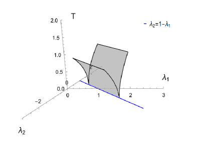
Figure 2: A sketch of a quantum critical line $\lambda_{2}=1-\lambda_{1}$, extended to finite temperature $T$.

.

There is a classic example of QCP, known as the transverse field Ising model in one dimension whose exact solution provides the properties of a quantum critical point addressed in detail in Ref. Sachdev, 2005. Experimentally, this model is well represented by $\mathrm{CoNb_{2}O_{6}}$,Kinross et al. (2014) which illustrates the nature of quantum criticality. Quantum critical lines (QCL) or surfaces (QCS) are less studied. We introduce a simple but exactly solved model of QCL and explore it in some detail. This model was introduced by Kopp and Chakravrty, Kopp and Chakravarty (2005) and has numerous exciting properties. It remains to be experimentally studied. The phase transitions in this model have intriguing topogical aspects discussed by Niu et al. Niu et al. (2012) to which we shall return in the text. We cannot overemphasaize the fact that subtle effects related to quantum fluctuations require an exact solution of the proposed model. It is hoped that an experimental realization will be found and studied. At the end we briefly remark on the Fermi surface as a QCS. The discussion is based on non-interacting fermions that reflect criticality because of the infinitely sharp nature of the fermi surface.

The paper is organized as follows: In Section II, we introduce the model and its quantum critical lines, and explore its properties in the context of QCL. In the following Section III we briefly touch upon Majorana representation, which was extensively discussed in the past Niu et al. (2012) and in Sec. IV the effect of disorder is treated, as any experimental realization will evidently involve randomness of model parameters. In Sec. V we briefly touch upon Fermi surface from the present perspective of criticality. The final Section VI is a summary.

II The Model and its quantum critical lines

The model we study is the three spin extension of the TFIM, studied previously by Kopp and Chakravarty (2005). We will focus on topics that was not studied previously. The Hamiltonian, $H$, is

$$H=-\sum_{i}(h_{i}\sigma_{i}^{x}+\lambda_{2}\sigma_{i}^{x}\sigma_{i-1}^{z}\sigma_{i+1}^{z}+\lambda_{1}\sigma_{i}^{z}\sigma_{i-1}^{z})$$ (1)

written in terms of standard Pauli matrices. In this section we discuss its phase diagram. We shall set $h_{i}=h=cst.$ The Hamiltonian after Jordan-Wigner Pfeuty (1970),Lieb et al. (1961) transformation

$$\sigma_{i}^{x}=1-2c_{i}^{\dagger}c_{i}$$ (2)

$$\sigma_{i}^{z}=-\prod_{j<i}(1-2c_{j}^{\dagger}c_{j})(c_{i}+c_{i}^{\dagger})$$ (3)

is

$$\begin{split}H&=-\sum_{i=1}^{N}h(1-2c_{i}^{\dagger}c_{i})-\lambda_{1}\sum_{i=1}^{N-1}(c_{i}^{\dagger}c_{i+1}+c_{i}^{\dagger}c_{i+1}^{\dagger}+h.c.)\\ &-\lambda_{2}\sum_{i=2}^{N-1}(c_{i-1}^{\dagger}c_{i+1}+c_{i+1}c_{i-1}+h.c.).\end{split}$$ (4)

In contrast to the spin model, the spinless fermion Hamiltonian is actually a one-dimensional mean field modelKitaev (2001) of a $p$-wave superconductor, but there are both nearest and next nearest neighbor hopping, as well as condensates—note the pair creation and destruction operators. The solution of the corresponding spin Hamiltonian through Jordan-Wigner transformation is, however, exact and includes all possible fluctuation effects and is not a mean field solution of any kind.

Imposing periodic boundary conditions, a Bogoliubov transformation results in its diagonalized form:

$$H=\sum_{k}2E_{k}\left(\eta_{k}^{\dagger}\eta_{k}-1\right).$$ (5)

As usual, the anticommuting fermion operators $\eta_{k}$’s are suitable linear combinations in the momentum space of the original Jordan-Wigner fermion operators. The spectra of excitations are (lattice spacing will be set to unity throughout the paper unless stated otherwise)

$$E_{k}=\sqrt{1+\lambda_{1}^{2}+\lambda_{2}^{2}+2\lambda_{1}(1-\lambda_{2})\cos k-2\lambda_{2}\cos 2k}$$ (6)

We haveset $h=1$ when discussing the zero temperature, $T=0$, properties.. At finite temperaures we must keep $h$ to be finite, similarly for the disordered system (cf. below). Quantum phase transitions of this model are given by the nonanalyticities of the ground state energy:

$$E_{0}=-2\sum_{k}E_{k}.$$ (7)

Taking the derivative of the energy dispersion, we get:

$$\frac{\partial E_{k}}{\partial k}=\frac{4\text{$\lambda_{2}$}\sin 2k-2\text{$\lambda_{1}$}(1-\text{$\lambda_{2}$})\sin k}{2\sqrt{2\text{$\lambda_{1}$}(1-\text{$\lambda_{2}$})\cos k-2\text{$\lambda_{2}$}\cos 2k+\text{$\lambda_{1}$}^{2}+\text{$\lambda_{2}$}^{2}+1}}$$ (8)

The derivative vanishes vanishes at $k=0,\pm\pi$ and $\cos k=\lambda_{1}(1-\lambda_{2})/4\lambda_{2}$. For these values of $k$ the spectra assume minimum values. The nonanalyticites are defined by the critical lines where the gaps collapse and the $T=0$ correlation length diverges; see Fig. 4. Note that the change in the number of Majorana zero modes at the end of the chain corresponds to topological phase transitions.

To follow the description below refer to Fig. 5. The contour plot of the square of the gap for $0\leq\lambda_{1}\leq 2$ and $0\geq\lambda_{2}\geq-1$ is given in Fig. 3. We enumerate below some of the features of the phase diagram and its associated critical lines:

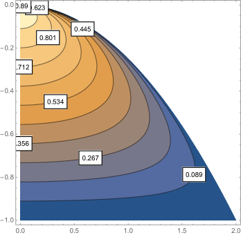
Figure 3: Contour plot of the square of the gap in the region $0\leq\lambda_{1}\leq 2$ and $0\geq\lambda_{2}\geq-1$

1. For the Ising model in a transverse field without three spin interaction, the gaps collapse at the Brillouin zone boundaries, $k=\pm\pi$ at the self-dual point $\lambda_{1}=1$ and $\lambda_{2}=0$.

2. As we move along the critical line $\lambda_{2}=1-\lambda_{1}$, there are no additional critical points until we reach $\lambda_{2}=1$ , then the gaps collapse at $k=0$ when $\lambda_{1}=0$ and $\lambda_{2}=1$, In the language of conformal field theory, this crossover is described by Zamolodchikov’s c-function’, which takes one from a theory of conformal charge $c=1$ to that of charge $c=1/2$. Castro Neto and Fradkin (1993) Then on $\lambda_{2}=1+\lambda_{1}$ constitutes a critical line with criticality at $k=0$.

3. When the three spin interaction is added, the gaps also collapse at $k=\cos^{-1}(\lambda_{1}/2)$ for $\lambda_{2}=-1$ and $0<\lambda_{1}<2$. This constitutes an unusual incommensurate critical line. At exactly $\lambda_{2}=-1$ and $\lambda_{1}=2$, the multicritical point is no longer Lorentz invariant and the dynamical exponent is $2$. This has important consequence in the spin-spin correlation function didcussed below because conformal invariance no longer holds.

4. In the dual representation discussed below, the region enclosed by $\lambda_{1}^{2}=-4\lambda_{2}$ is an oscillatory ferromagnetically ordered phase separating from an ordered phase for $\lambda_{2}<0$, as determined by the spatial decay of the instantaneous spin-spin correlation function. This does not reflect a critical line, however.Barouch and McCoy (1971)

5. It is easy to compute specific heat, $C$, which is linearly proportional to $T$, as $T\to 0$, on all critical lines except at the multicritical point $(d)$ in Fig. 4; $C$ vanishes as $T^{1/2}$. The theory at this point is not conformally invariant. Disorder has a strong effect at this point as well, as we shall see later.

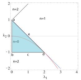
Figure 4: The phase diagram, $n=0,1,2$ correspond to regions with $n$ Majorana zero modes at each end of an open chain. The quantum critical lines are determined by the vanishing of the energy gaps. The points (a) and (d) are multicritical points. The thin green line is a disorder line of no significance to quantum criticality. Niu et al. (2012)

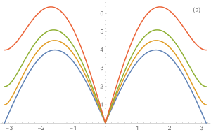
Figure 5: 2$E_{k}$ versus momentum $k$. The critcality along (a) $\lambda_{2}=1-\lambda_{1}$: top to bottom $\lambda_{1}\to 0$, (b) $\lambda_{2}=1+\lambda_{1}$ where $\lambda_{1}$ varies between $0$ and $1$, (c) $\lambda_{2}=-1,0\leq\lambda_{1}\leq 2$, plotted in the interval between $0$ and $2\pi$.

But at the free fermion point $b$, there are no zero energy excitations except at $k=\pm\pi/2$. When we move to the point $c$ the spectrum evolves increasing the weight at $k=0$ and the locations of the nodes are incommensurate with the lattice. The incommensuration shifts as a function of $\lambda_{1}$. The point $d$ is a multicritical point, with the dynamical critical point $z=2$ and the spectra vanishes quadratically at $\pm\pi$. The spectra are no longer relativistic at this point as a result of the confluence of two Dirac points, corresponding to a dynamical exponent $z=2$ and the correlation length exponent $\nu=1/2$. The multicritacl point at $a$ still corresponds to dynamical exponent $z=1$, but its location is now at $k=0$. The linearly vanishing spetrum continues as $\lambda_{1}=1+\lambda_{2}$ located at $k=0$.

II.1 The dual representation

In this section we exhibit the dual representation, which shows that the model is also dual to an anistropic $XY$-model with a magnetic field in the $z$-direction. We show the transcription in case the $XY$-version is better realized from tht possible experimental perspective.

Let us define the dual operators:

$$\mu_{x}(n) = \sigma_{z}(n+1)\sigma_{z}(n),$$ (9)

$$\mu_{z}(n) = \prod_{m\leq n}\sigma_{x}(m),$$ (10)

which implies that

$$[\mu_{z}(n),\mu_{x}(n)] = -2i\mu_{y}(n),$$ (11)

$$\mu_{y}(n) = -i\bigg{(}\prod_{m\leq n}\sigma_{x}(m)\bigg{)}\sigma_{z}(n+1)\sigma_{z}(n).$$ (12)

The Hamiltonian under duality transforms to

$$\begin{split}H_{D}&=-\frac{2}{1+r}\sum_{n}\bigg{[}\frac{1+r}{2}\mu_{x}(n)\mu_{x}(n+1)\\ &+\frac{1-r}{2}\mu_{y}(n)\mu_{y}(n+1)+h\mu_{z}(n))\bigg{]},\end{split}$$ (13)

where we have carried out the rotations : $\mu_{x}(n)\to\mu_{z}(n)$, $\mu_{z}(n)\to\mu_{x}(n)$, $\mu_{y}(n)\to-\mu_{y}(n)$. The parameters are related by

$$\lambda_{1}=\frac{2h}{1+r},\;\lambda_{2}=\frac{r-1}{1+r}.$$ (14)

The critical line in the $XY$-model, separating the quantum disordered phase from the ferromagnetic phase is at $h=1$, which corresponds to $\lambda_{1}+\lambda_{2}=1$, separating the ordered phase from the disordered phase. Since the ordered and the disordered phases are exchanged under duality, the disordered phase of the three-spin model is $\lambda_{1}+\lambda_{2}<1$.

III Majorana representatrion

The phase transitions in this model in the superconducting version (in the fermion language) is best described in terms of Majorana zero modes at the end of the one-dimensional chain. This view was discussed in detail in a previous paper. Niu et al. (2012) While in the spin language the phases are described in the traditional language of an order parameter, ferromagnetic or quantum disordered states, in the fermion language, the system is always a superconductor, except that the states are either BCS or BEC phases. That there is a phase transition between the two is a reflection of the topological nature of the states. Referring to Fig. 4, the winding numbers $n=0,1,2$ are the number of zero energy Majorana modes at each end of the chain. These windings were explained in terms of the Anderson pseudospin Hamiltonian, Anderson (1958) when the time reversal symmetry is respected. In the absence of time reversal symmetry, the two Majorana zero modes can hybridize and split. The change in the winding numer cannot take place without a phase transition. More recently, the topological nature was brought out by the notion of curvature renormalization group (CRG)Kumar et al. (2021); Abdulla et al. (2020) that may be useful in higher dimensional systems. Here there is an exact solution of the model.

IV Dynamical structure factor

We examine both pure and disordered versions at zero temperature. For this purpose we compute spin-spin correlation function, which is possible to determine by Neutron scattering experiments.. It is difficult to find a suitable experimental technique in the superconducting picture, except perhaps by scanning tunneling microscopy—a topic that we would like to return in the future. The dynamical structure factor $S(k,\omega)$ can be measured in neutron scattering experiment. It is fortunate that we can provide a numerically exact method in this respect. Alternately one can also explore NMR relaxation rate.

For a pure system, $S(k,\omega)$ it contains no more information beyond the results for the excitation spectrum, but it encourages the experimentalists to perform the neutron measurements by measuring the spin-spin correlation function. Secondly, the method of calculation of the correlation function for the pure system can be tested before we consider the more complex disordered systems. Another important point is that it is rare that one can compute the real-time correlation function. In the present problem, this is possible because we have the full exact spectrum regardless of whether or not we have a pure or disordered case.

We treat two different models of disorder: the binary and the uniform distributions. The binary distribution consists of a large field $h_{L}$ and a small field $h_{S}$, with the probability distributions such that $P_{L}+P_{S}=1$ where

$$h_{i}=\begin{cases}h_{L}&\text{with probability $P_{L}$}\\ h_{S}&\text{with probability $P_{S}$}\end{cases}$$ (15)

in this case we keep $\lambda_{1}$ and $\lambda_{2}$ spatially independent. The probability distribution $P(h)$ for the binary distribution is

$$P(h)=P_{L}\ \delta(h-h_{L})+P_{S}\ \delta(h-h_{S})$$ (16)

The uniform distribution for $h$ is given by its average and the width

$$P(h_{i})=\begin{cases}1/h_{W},&h_{i}\in[h_{ave}-\frac{1}{2}h_{W},h_{ave}+\frac{1}{2}h_{W}]\\ 0,&\text{otherwise. }\end{cases}$$ (17)

IV.1 Correlation function in terms of a Pfaffian

We discuss the calculations in some detail for the reader to be able to repeat the calculation with ease, if necessary. Quite generally, the spin-spin correlation function $C_{ij}(t)$ is defined as

$$C(r,t)=\left<\sigma_{i}^{z}(t)\sigma_{j}^{z}(0)\right>$$ (18)

where $i$, $j$ are lattice sites and $r$ is the separation between them. The dynamical structure factor $S(k,\omega)$ is the time and space Fourier transformation of $C_{ij}(t)\equiv C(j-i,t)\equiv C(r,t)$. In a finite system of length $L$, we choose $i,j$ in the middle of the chain to reduce the boundary effects. Thus,

$$S(k,\omega)=\int dt\int dr\ e^{i\omega t}e^{-ikr}C(r,t).$$ (19)

The integral over $r$ represents of course a discrete sum on a lattice. Furthermore, for the disordered case we compute

$${\overline{C}(r,t)}=\overline{<\sigma_{i}^{z}(t)\sigma_{j}^{z}(0)>}$$ (20)

where the overline stands for an average over the disorder ensemble. The dynamical structure factor $S(k,\omega)$ is

$$S(k,\omega)=\int dt\int dr\ e^{i\omega t}e^{-ikr}C(r,t)$$ (21)

Using the Jordan-Wigner transformation, Eq. 3, we getLieb et al. (1961)

$$C(r,t)=\left<(\prod_{m=1}^{i-1}(c_{m}^{\dagger}+c_{m})(t)(c_{m}^{\dagger}-c_{m})(t))(c_{i}^{\dagger}+c_{i})(t)(\prod_{l=1}^{j-1}(c_{l}^{\dagger}+c_{l})(c_{l}^{\dagger}-c_{l}))(c_{j}^{\dagger}+c_{j})\right>$$ (22)

Because of the free fermion nature of the Jordan-Wigner transformed Hamiltonian, we can apply Wick’s theorem to $C(r,t)$. After collecting all terms in the Wick expansion, this gives us a Pfaffian. It means that

$$\left<\sigma_{i}^{z}(t)\sigma_{j}^{z}(0)\right>=Pf(S)$$ (23)

Here $S$ is a $2(i+j-1)$ dimensional skew-symmetric matrix. If we identify $A_{m}=c_{m}^{\dagger}+c_{m}$ and $B_{n}=c_{n}^{\dagger}-c_{n}$ The dmatrix $S$ is

$$S=\begin{pmatrix}0&<A_{1}(t)B_{1}(t)>&<A_{1}(t)A_{2}(t)>&<A_{1}(t)B_{2}(t)>&...&<A_{1}(t)A_{j}>\\ -<A_{1}(t)B_{1}(t)>&0&<B_{1}(t)A_{2}(t)>&<B_{1}(t)B_{2}(t)>&...&<B_{1}(t)A_{j}>\\ -<A_{1}(t)A_{2}(t)>&-<B_{1}(t)A_{2}(t)>&0&<A_{2}(t)B_{2}(t)>&...&<A_{2}(t)A_{j}>\\ \vdots&\vdots&\vdots&\vdots&\ddots&\vdots\\ -<A_{1}(t)A_{j}>&-<B_{1}(t)A_{j}>&-<A_{2}(t)A_{j}>&-<B_{2}(t)A_{j}>&...&0\end{pmatrix}$$ (24)

All we need to compute is the two point correlation functionFetter and Walecka (1971) such as

$$\left<(c_{m}^{\dagger}(t)\pm c_{m}(t))(c_{l}^{\dagger}\pm c_{l})\right>.$$ (25)

Here are the details of the remaining part of the calculation.. The matrix form of the Hamilitonian in the fermion basis is

$$H=\begin{matrix}\begin{pmatrix}c^{\dagger}&c\end{pmatrix}\end{matrix}\begin{pmatrix}A&B\\ -B&-A\end{pmatrix}\begin{pmatrix}c\\ c^{\dagger}\end{pmatrix}$$ (26)

in which $c=(c_{1},c_{2}.....c_{L})$, $c^{\dagger}=(c_{1}^{\dagger},c_{2}^{\dagger}.....c_{L}^{\dagger})$, $A$ and $B$ are both $L\times L$ matrices, whose elements are

$$A_{ij} = \lambda_{1}(\delta_{j,i+1}+\delta_{j,i-1})+\lambda_{2}(\delta_{j,i+2}+\delta_{j,i-2})-2h_{i}\delta_{ij}$$ (27)

$$B_{ij} = -\lambda_{1}(\delta_{j,i+1}-\delta_{j,i-1})-\lambda_{2}(\delta_{j,i+2}-\delta_{j,i-2})$$ (28)

Now, we diagonalize $H$ as

$$H=\begin{matrix}\begin{pmatrix}c^{\dagger}&c\end{pmatrix}\end{matrix}VDV^{-1}\begin{pmatrix}c\\ c^{\dagger}\end{pmatrix}=\begin{matrix}\begin{pmatrix}\eta^{\dagger}&\eta\end{pmatrix}\end{matrix}D\begin{pmatrix}\eta\\ \eta^{\dagger}\end{pmatrix}$$ (29)

Here $D$ and $V$ are $2L\times 2L$ matrices that take the following forms:

$$D=\begin{bmatrix}E_{1}&\\ &E_{2}&\\ &&E_{3}\\ &&&...\\ &&&&...\\ &&&&&E_{2L}\end{bmatrix},$$ (30)

$$V=\begin{pmatrix}X_{L\times L}&Y_{L\times L}\\ Y_{L\times L}&X_{L\times L}\end{pmatrix}$$ (31)

$(X)_{L\times L}$ means a $L\times L$ matrix. Now, our Hamilionian in the basis of $\eta$ and $\eta^{\dagger}$ above should becomes

$$H=\sum_{\mu=1}^{L}2E_{\mu}\left(\eta_{\mu}^{\dagger}\eta_{\mu}-1\right).$$ (32)

We represent everything in real-space since momentum representation in Eq.(9) doesn’t work in the disorder case; $\mu$ is no longer the momentum quantum number. The first term is the diagonalized Hamilitonian and the second term is the ground state energy. Next, in order to evaluate Eq.(28), we need to rewrite $c^{\dagger}$ and $c$ in terms of $\eta^{\dagger}$ and $\eta$. Since $\begin{pmatrix}c\\ c^{\dagger}\end{pmatrix}=V\begin{pmatrix}\eta\\ \eta^{\dagger}\end{pmatrix}$, we have

$$\begin{pmatrix}c^{\dagger}+c\\ c^{\dagger}-c\end{pmatrix}=\begin{pmatrix}X+Y&0\\ 0&X-Y\end{pmatrix}\begin{pmatrix}\eta^{\dagger}+\eta\\ \eta^{\dagger}-\eta\end{pmatrix}.$$ (33)

Evaluation of Eq.(27) requires all possible $m$ and $l$ in Eq.(28). A nice way to do this is to rewrite Eq.(28) as a $2L\times 2L$ matrix called $C_{t}$ whose elements contain all possible two points correlators.

$$C_{t}=\left<\begin{pmatrix}c^{\dagger}(t)+c(t)\\ c(t)-c^{\dagger}(t)\end{pmatrix}\begin{pmatrix}c^{\dagger}+c&c-c^{\dagger}\end{pmatrix}\right>$$ (34)

Here $c+c^{\dagger}\equiv(c_{1}+c_{1}^{\dagger},c_{2}+c_{2}^{\dagger},.....,c_{L}+c_{L}^{\dagger})$. Then we use Eq.(36) to get

$$\left<\begin{pmatrix}c^{\dagger}(t)+c(t)\\ c(t)-c^{\dagger}(t)\end{pmatrix}\begin{pmatrix}c^{\dagger}+c&c-c^{\dagger}\end{pmatrix}\right>=\begin{pmatrix}X+Y&0\\ 0&X-Y\end{pmatrix}\left<\begin{pmatrix}\eta^{\dagger}(t)+\eta(t)\\ \eta(t)-\eta^{\dagger}(t)\end{pmatrix}\begin{pmatrix}\eta^{\dagger}+\eta&\eta-\eta^{\dagger}\end{pmatrix}\right>$$ (35)

$$\begin{pmatrix}X^{\dagger}+Y^{\dagger}&0\\ 0&X^{\dagger}-Y^{\dagger}\end{pmatrix}$$

Now We just need to evaluate $\left<\begin{pmatrix}\eta^{\dagger}(t)+\eta(t)\\ \eta(t)-\eta^{\dagger}(t)\end{pmatrix}\begin{pmatrix}\eta^{\dagger}+\eta&\eta-\eta^{\dagger}\end{pmatrix}\right>$.

We calculate that by first computing $\left<\begin{pmatrix}\eta(t)\\ \eta^{\dagger}(t)\end{pmatrix}\begin{pmatrix}\eta^{\dagger}&\eta\end{pmatrix}\right>$. Here $\eta(t)\equiv(\eta_{1}(t),\eta_{2}(t),.....,\eta_{L}(t))$. Fortunately, the only non-zero contraction is between $\eta_{i}(t)$ and $\eta_{j}^{\dagger}$. It gives $\left<\eta_{i}(t)\eta_{j}^{\dagger}\right>=\delta_{ij}e^{i2E_{i}t}$, Now our matrix $C_{t}$ becomes

$$C_{t}=\begin{pmatrix}X+Y&0\\ 0&X-Y\end{pmatrix}\begin{pmatrix}(\delta_{ij}e^{i2E_{i}t})_{L\times L}&-(\delta_{ij}e^{i2E_{i}t})_{L\times L}\\ -(\delta_{ij}e^{i2E_{i}t})_{L\times L}&(\delta_{ij}e^{i2E_{i}t})_{L\times L}\end{pmatrix}\begin{pmatrix}X^{\dagger}+Y^{\dagger}&0\\ 0&X^{\dagger}-Y^{\dagger}\end{pmatrix}$$ (36)

Then, if one finds $X$ and $Y$ correctly, we are able to compute $C_{t}$ without any difficulty. However, getting those eigenvectors $X$ and $Y$ from exact diagonalization of $H$ is not numerically stable (suffers large errors) if their eigenvalues are very close to zero. Thus, instead of directly diagonalizing our $2L\times 2L$ hamilitonian, we choose to use singular value decomposition (SVD)Press et al. (2007) to diagonalize $L\times L$ matrix. To this end, we change our basis from $c$ and $c^{\dagger}$ into $c^{\dagger}+c$ and $c^{\dagger}-c$; our Hamilitonian transforms to

$$\widetilde{H}=\begin{pmatrix}c^{\dagger}+c&c-c^{\dagger}\end{pmatrix}\begin{pmatrix}0&M^{T}\\ M&0\end{pmatrix}\begin{pmatrix}c^{\dagger}+c\\ c^{\dagger}-c\end{pmatrix}$$ (37)

in which $M=-\frac{(A+B)}{2}$ and $M^{T}=-\frac{(A-B)}{2}$.

The exact form of $M$ is

$$M=\begin{bmatrix}h_{1}&-\lambda_{1}&-\lambda_{2}&&\\ &h_{2}&-\lambda_{1}&-\lambda_{2}&&\\ &&h_{3}&-\lambda_{1}&\ddots&\\ &&&\ddots&\ddots&-\lambda_{2}\\ &&&&\ddots&-\lambda_{1}\\ &&&&&h_{L}\end{bmatrix}$$ (38)

Next we apply SVD to matrix $M$. This gives us

$$M=\psi\Lambda\phi^{T}$$ (39)

where $\psi$ and $\phi$ are $L\times L$ orthogonal matrices and $\Lambda$ is diagonal with non-negative entries. The SVD also implies

$$M\phi=\psi\Lambda$$ (40)

$$M^{T}\psi=\phi\Lambda$$ (41)

Those are equivalent to the equation

$$\widetilde{H}\begin{pmatrix}\phi&\phi\\ \psi&-\psi\end{pmatrix}=\begin{pmatrix}\phi&\phi\\ \psi&-\psi\end{pmatrix}\begin{pmatrix}\Lambda&0\\ 0&-\Lambda\end{pmatrix}$$ (42)

Then one can show the equivalence between $X+Y$, $X-Y$ and $\phi$, $\psi$ in SVD. We have

$$\begin{pmatrix}\phi&0\\ 0&\psi\end{pmatrix}=\begin{pmatrix}X+Y&0\\ 0&X-Y\end{pmatrix}$$ (43)

Finally, our two point fermion-fermion correlation function becomes

$$C_{t}=\left<\begin{pmatrix}c^{\dagger}(t)+c(t)\\ c(t)-c^{\dagger}(t)\end{pmatrix}\begin{pmatrix}c^{\dagger}+c&c-c^{\dagger}\end{pmatrix}\right>=\begin{pmatrix}\phi&0\\ 0&\psi\end{pmatrix}\begin{pmatrix}(\delta_{ij}e^{i2E_{i}t})_{L\times L}&-(\delta_{ij}e^{i2E_{i}t})_{L\times L}\\ -(\delta_{ij}e^{i2E_{i}t})_{L\times L}&(\delta_{ij}e^{i2E_{i}t})_{L\times L}\end{pmatrix}\begin{pmatrix}\phi^{\dagger}&0\\ 0&\psi^{\dagger}\end{pmatrix}$$ (44)

Now, we can get all elements in matrix $S$ by mapping to all elements in $C_{t}$. But we still need to deal with one last issue. The computation of a Pfaffian consumes a lot of time by standard methods for a large-sized system. An efficient method for calculating such Pfaffians was invented in a previous paper.Jia and Chakravarty (2006) Let $X$ be a $2N\times 2N$ skew-symmetric matrix which has the following form

$$X=\left[{\begin{array}[]{cc}A&B\\ -B^{T}&C\\ \end{array}}\right]$$ (45)

where $A$ is a $2\times 2$ matrix, and $B$ and $C$ are matrices of appropriate dimensions.Then we have the identity

$$\left[{\begin{array}[]{cc}I_{2}&0\\ B^{T}A^{-1}&I_{2N-2}\\ \end{array}}\right]X\left[{\begin{array}[]{cc}I_{2}&-A^{-1}B\\ 0&I_{2N-2}\\ \end{array}}\right]=\left[{\begin{array}[]{cc}A&0\\ 0&C+B^{T}A^{-1}B\\ \end{array}}\right]$$ (46)

where $I_{n}$ is a $n\times n$ identity matrix, and

$$\mathrm{det}(X)=\mathrm{det}(A)\mathrm{det}(C+B^{T}A^{-1}B)$$ (47)

This gives us an iteration method. We will get a $2\times 2$ matrix $A$ in each iteration step; we treat $C+B^{T}A^{-1}B$ to be our next $X$ and keep doing this. Our $\det(X)$ eventually becomes a product chain of $2\times 2$ matrices.

IV.2 Pure System

The calculations in this section were performed on a chain that has 128 lattice sites with free boundary conditions. We always choose 64 sites in the middlke to compute the correlation function. In the pure model, we focus on how dynamical structure factor $S(k,\omega)$ evolves along the line $\lambda_{2}=1\pm\lambda_{1}$ as represented in Fig. 6. In addition, we also plot the result as we tune $\lambda_{1}$ to the multicritical point $\lambda_{1}=2$ and $\lambda_{2}=-1$; see Fig.7. Possible neutron scattering will measure spin-spin correlation function. It is satisfying to see that the spectra still correctly represent the fermionic excitations. It is of course not possible to directly couple to the Jordan-Wigner fermions. In addition it is a good test that our calculations are reliable and we can safely continue to the disorder problem

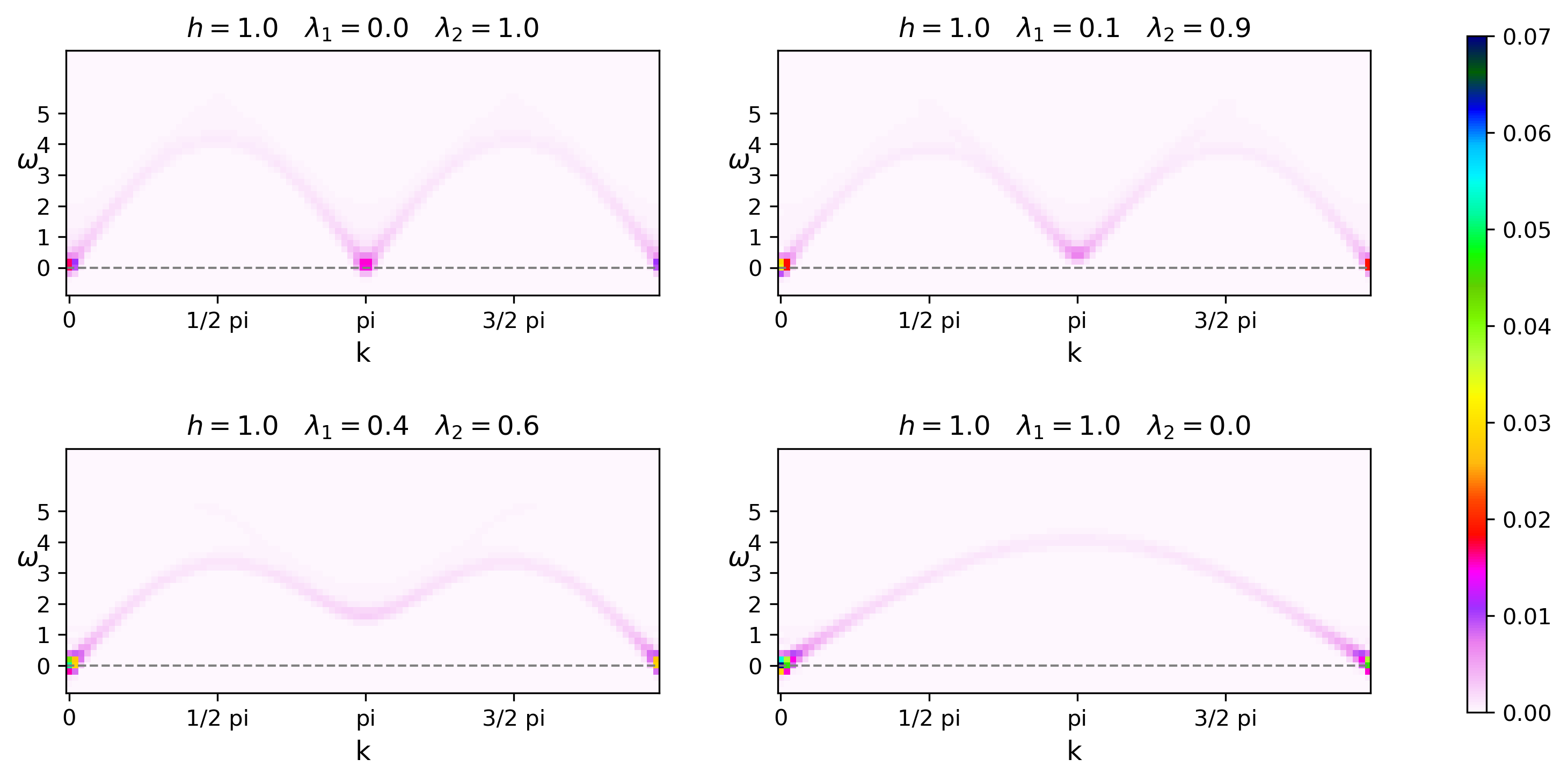
Figure 6: Normalized dynamical structure factor $S(k,\omega)$ calculated at four points..

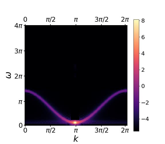
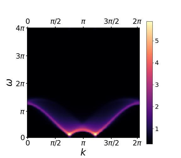
Figure 7: Top: Dynamical structure factor $S(k,\omega)$ calculated at the multicriitical point $\lambda_{2}=-1$ and $\lambda_{1}=2$; Bottom:.$\lambda_{2}=-1$ and $\lambda_{1}=1.5$.

IV.3 Disordered System

A cursory look at Eq. 4 would seem that the disorder in this one dimensional model will result in Anderson localization of the fermionic states. This not true because the Hamltonian contains pair creation and destruction operators; it corresponds to a model of a superconductor, in which charge is not conserved.

Computation of $S(k,\omega)$ involves averaging of the correlation function. We found that there appears to be no difference between configuration averages of 1000 and 3000 samples. A representative set of $S(k,\omega)$ are shown in Figs. 8,9,10,11. This example corresponds to little disorder and therefore very little broadening and the dispersions remains intact.

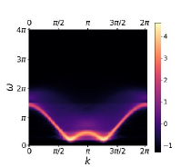
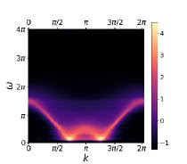
Figure 8: Dynamical structure factor $S(k,\omega)$ calculated for a uniform disorder. Top: $\lambda_{2}=-1$ and $\lambda_{1}=1.5,h_{w}=1$; Bottom: $h_{w}=2$.

For higher values of disorder the dispersion breaks up as shown in Fig. 9 and Fig. 10. .

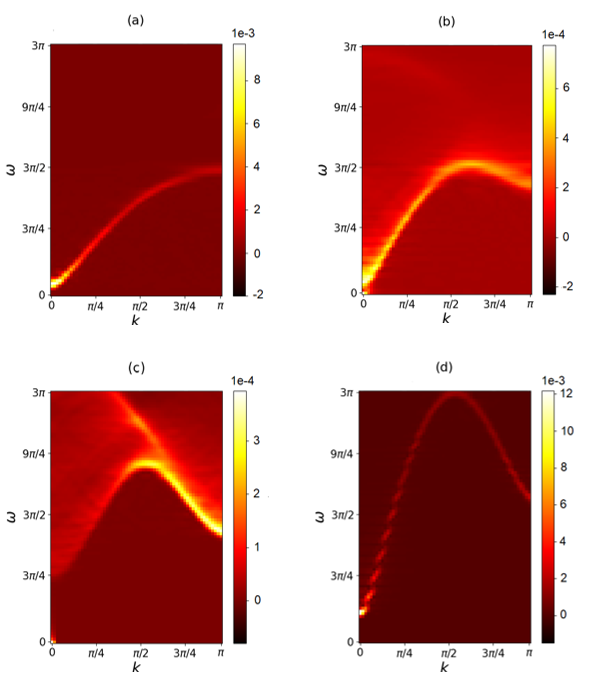
Figure 9: Normalized dynamical structure factor $S(k,\omega)$ with increasing value of $\lambda_{2}$ for uniform disorder. The parameters are $\lambda_{1}=1$, $h_{av}=1.4$ and $h_{w}=0.5$: $\lambda_{2}=(a)\;0.1,(b)\;0.5,(c)\;1.0,(d)\;3.0$.

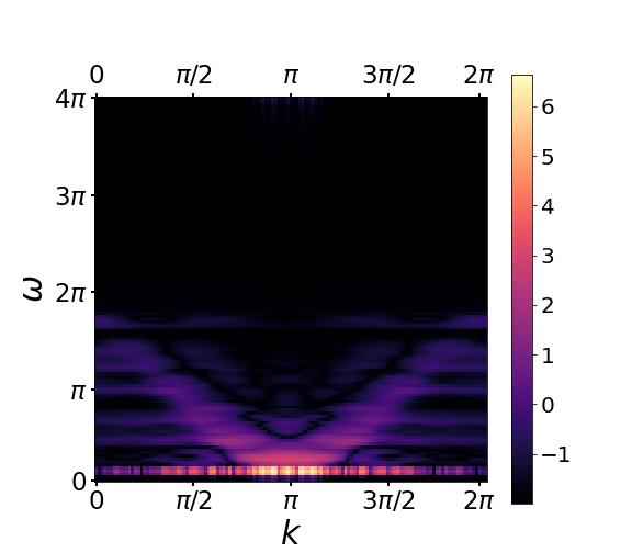
Figure 10: The parametersare $\lambda_{1}=2,\lambda_{2}=-1,h_{L}=3$, $h_{S}=1$, $P_{L}=0.1$ at the multicritical point. The quadratic dispersion is still visible.

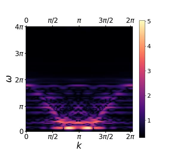
Figure 11: The parameters are $\lambda_{1}=2,\lambda_{2}=-1,h_{L}=3$, $h_{S}=1$, $P_{L}=0.5$. The dispersion is broken up for large disorder.

V Fermi surface

It is amusing to note that from the perspective of quantum criticality, the “normal” state is the superconducting state with a gap, $\Delta$ tied to the Fermi surface; the Fermi surface is obtained when the superconducting gap collapses: $\Delta(\lambda_{1},\lambda_{2},\lambda_{3}\ldots)=0$, where $\lambda_{1},\lambda_{2},\lambda_{3},\ldots$ are possible coupling constants. The surface spanned by more than two coupling constants could of course be described as a quantum critical surface. In the case of BCS theory, only one coupling constant is relevant, in which case the critical surface converts to a QCP. The essence of Kohn-Luttinger theoryKohn and Luttinger (1965) of superconductivity is that all Fermi systems, whether or not attractive or repulsive, has the ground state that is superconducting (as long as spatial inversion, time-reversal, or both symmetries are respected). The important point in our present context is the collapse of the gap, not the applicability of the BCS theory.

The Fermi surface viewed as a critical surface has been discussed in great detail by VolovikVolovik (2003) from the perspective of a topological object in the momentum space. The singularities of the Green function in $(p_{0},{\bf p})$ frquency-momentum space is topologically equivalent to a quantized vortex in ($3+1$-dimensional) spacetime $({\bf r},t)$.

The important point about the Fermi surface is its lack of scale; it is infinitely sharp. As long as the modes do not couple, there are no phenomena that are out of the ordinary. But when they do, we run into important effects, as in the Kondo problem.Wilson (1983) However, some aspect of criticality of the Fermi surface can be gleaned from an elementary calculationLandau and Lifshitz (1980) of density-density correlation function of a Fermi system:

$$\left<\Delta n_{1}\Delta n_{2}\right>=\overline{n}\delta({\bf r}_{2}-{\bf r}_{1})+\overline{n}\nu(r),$$ (48)

where $\overline{n}$ is the average density, and $\Delta n(r)=(n(r)-\overline{n})$,

$$\nu(r)=-\frac{g}{\overline{n}}\left|\int\frac{d^{3}p}{(2\pi\hbar)^{3}}\frac{e^{i{\bf p}\cdot{\bf r/}\hbar}}{e^{(\varepsilon_{p}-\mu)/T}+1}\right|^{2},$$ (49)

$g=(2S+1)$; $S$ is the spin. As $T\to 0$, and $p_{F}r/\hbar$ is large compared to $\varepsilon_{F}/T$ and also with respect to unity:

$$\nu(r)\approx-\frac{3T^{2}}{\hbar v_{F}^{2}p_{F}r^{2}}\exp\left(-\frac{2\pi Tr}{\hbar v_{F}}\right).$$ (50)

Here $v_{F}$ is the Fermi velocity and $p_{F}$ is the Fermi momentum. The criticality of the Fermi surface is manifest in the correlation length $\xi=\hbar v_{F}/2\pi T$, which diverges as $T\to 0$. The corresponding time scale is given by

$$\tau=\frac{\xi}{v_{F}}=\frac{\hbar}{2\pi T},$$ (51)

which is an elementary example of what is known as planckian time discussed in the recent literature. Zaanen (2019); Hartnoll and Mackenzie (2022) The above result is typical of a gapless system, and is applicable to many physical systems; see, for example, the $(2+1)$-dimensional quantum Heisenberg model. Chakravarty et al. (1989) This Planckian time is not the momentum relaxation time in a Fermi liquid, $1/\tau_{F}\propto A(1/\hbar)T^{2}/\varepsilon_{F}$, as discussed in textbooks.Ashcroft and Mermin (1976) $A$ is a dimensionless constant.

VI Summary

In this paper we have have explored an exactly solved model that exhibits three interesting quantum critical lines and two multicritical points. The centerpiece is the notion that the existence of quantum critical lines allow one to explore zero temperature quantum critical fluctuations without excessive fine tuning, as would be the case for a quantum critical point. The three lines have their unique characteristics. On one line criticality is unchanged and are located at $k=\pm\pi$ ($\nu=1,z=1$), in the other it is centered at $k=0$ ($\nu=1,z=1$), and in the third the criticality is at incommensurate $k$-points. It is remarkable that the same model can exhibit such varied behavior. In addition there two multicritical points. One of which corresponds to nonrelativistic quadratic dispersion with a dynamical exponent $z=2$ and a critical exponent $\nu=1/2$. The specific heat on all critical lines except at the multicritical point $(d)$ in Fig. 4 is linear in $T$ with differing slopes; at this multicritical point, the specific heat is proportional to $\sqrt{T}$.

The transition lines at $T=0$ are topological in the sense that the number of Majorana zero modes at each end of the chain changes across the transition lines. Since all realistic physical examples must involve some degree of disorder, we explored its effects on the dispersion spectrum. It is quite fortunate that the real-time spectra can be calculated because the model is exactly solved. Typically it is difficult to calculate the real-time spectra.

We believe that experimental realizations of the model can be found in which a free chain is all that is needed. Perhaps experimental techniques of NMR relaxation methodsKinross et al. (2014) as well as terahertz spectroscopy could be employed.Morris et al. (2014); Xu et al. (2022) The artifact of periodic boundary condition is not necessary, simplifying the search for a physical model.

It is possible to extend our model by adding further neighbor interactions, still maintaining its exact solvability, so as to discuss quantum critical surfaces in the parameter space. However, experimental realizations of such models will be increasingly difficult to achieve. Finally, QCS that is only cursorily mentioned here could be found in the language of gauge-gravity dual ideas.Zaanen et al. (2015)