The nature of visons in the perturbed ferromagnetic and antiferromagnetic Kitaev honeycomb models

Abstract

The Kitaev honeycomb model hosts a fascinating fractionalized state of matter featuring emergent Majorana fermions and a vison particle that carries the flux of an emergent gauge field. In the exactly solvable model these visons are static but certain perturbations can induce their motion. We show that the nature of the vison motion induced by a Zeeman field is sharply distinct in the ferromagnetic vs the antiferromagnetic Kitaev models. Namely, in the ferromagnetic model the vison has a trivial non-projective translational symmetry, whereas in the antiferromagnetic Kitaev model it has a projective translational symmetry with $\pi$-flux per unit cell. The vison band of the ferromagnetic case has zero Berry curvature, and no associated intrinsic contribution to the thermal Hall effect. In contrast, in the antiferromagnetic case there are two gapped vison bands with opposite Chern numbers and an associated intrinsic vison contribution to the thermal Hall effect. We discuss these findings in the light of the physics of the spin liquid candidate $\alpha$-RuCl₃.

I Introduction

The Kitaev honeycomb model [1] has become a paradigmatic playground to investigate spin liquids with emergent fermions and $Z_{2}$ gauge fields in two-dimensions. Unlike other exactly solvable models, the model only contains spin bilinears and it is believed to be a reasonable description of certain quantum magnets, such as $\alpha$-RuCl₃ [2, 3, 4]. Although $\alpha$-RuCl₃ forms a zig-zag antiferromagnet in the absence of applied magnetic fields [5, 6, 7], there are several experimental indications that it might harbor a quantum spin liquid once an in-plane magnetic field is applied within a range of $\sim 6T-11T$ [8, 9, 10, 11, 12, 13, 14, 15, 16, 17, 18].

Nevertheless, the connection between the experimentally observed potential spin-liquid in $\alpha$-RuCl₃ and the spin liquids realized in the weakly perturbed ideal Kitaev model is currently far from clear. This stems in part from the lingering uncertainty on the minimal Heisenberg-type model describing the material. The largest coupling term in $\alpha$-RuCl₃, denoted by $K$, is in fact believed to be the term that appears in the ideal Kitaev model. While a majority studies have advocated that this coupling is ferromagnetic (FM, $K<0$), others have advocated for an antiferromagnetic (AFM, $K>0$) exchange coupling (see Refs. [19, 20] for tables summarizing the estimates of several studies). Some of the prominent observational evidence favoring $K$ to be ferromagnetic come from elastic X-ray scattering experiments [21] that determined the direction of the ordered moment in the zig-zag AFM state, which is dependent on the sign of $K$ [22]. Inelastic X-ray scattering experiments [23] have also advocated for a ferromagnetic coupling. However, these experiments relied on modeling the zig-zag AFM state, which is highly susceptible to perturbations and itself subjected to very strong quantum fluctuations. Therefore we believe that there is still some room to be reasonably skeptic about the certainty of the sign of this coupling. Determining this sign is crucial for many reasons. For example the spin liquid realized in the AFM coupled case is more robust to certain perturbations, as compared to the spin liquid realized for the FM coupled case [24, 25, 26, 27]. Additionally, the nature of the phases driven by the applied Zeeman field can be very different in both cases, displaying a delicate dependence on the further-neighbor exchange couplings allowed by symmetry, such as the $\Gamma,\Gamma^{\prime},J,J_{3}$ terms [28, 29, 24, 25, 26, 27, 19, 20, 30, 31, 26].

In the present study we will further emphasize the importance of the sign of $K$ by demonstrating that the FM Kitaev model is in a sharply distinct topological phase compared to the AFM Kitaev model in the presence of a Zeeman field. More specifically, we will show that even though the FM and AFM Kitaev models realize ground states within the same celebrated Ising topological order, they realize distinct symmetry enriched topological orders with regard to the translational symmetry of the lattice, and therefore belong to two distinct universality classes. This distinction manifests vividly on the properties of its vison quasiparticle [32, 33, 34, 35], which is the emergent non-abelian anyon analogous to a $\pi$-flux in a $p+ip$ superconductor that carries a Majorana fermion zero mode in its core [36].

We will show that for the FM Kitaev model, lattice translations act on the vison in an ordinary non-projective way. This implies that the vison Bravais lattice contains a single state per unit cell associated with each hexagon of the honeycomb lattice (see Fig. 1(a)), and as a consequence its Berry curvature vanishes everywhere in its Brillouin zone. One important aspect that we will emphasize in our study is that in order to correctly capture the motion of the vison induced by the Zeeman field, it is crucial to include the Haldane mass term that is generated perturbatively by the Zeeman field on the itinerant Majorana fermions. Such a term is strictly necessary in order to make the state a fully gapped topologically ordered phase of matter and to make the vison an exponentially localized particle. In fact, we will directly show numerically that in finite size systems the phase that the vison acquires is highly sensitive on system size and boundary conditions when the Haldane mass of the Majorana is set to be exactly zero. On the other hand, we will also show numerically that as the thermodynamic limit is approached any small but non-zero Haldane mass term is sufficient in order to regularize and obtain a unique and well defined phase for the visons as they moves around a unit cell of the Bravais lattice.

On the other hand, we will show that for the AFM Kitaev model the presence of the Haldane mass term leads to a finite vison hopping. We will show that interestingly in the AFM case the vison has indeed projective translations with $\pi$-flux per unit cell allowing it to have a finite Berry curvature and two Chern bands with Chern numbers $C{\,=\,}\pm 1$. We will also show, in agreement with Ref. [37], that perturbatively in the applied Zeeman field, the vison in the FM Kitaev model has a larger band-width than in the AFM Kitaev model, so the vison band minimum reaches zero faster in the former (FM) case as the Zeeman field increases (see Fig. 5 for a plot of vison bands in both FM and AFM Kitaev models). This is crucially related to the stability of the latter against Zeeman perturbations that would stabilize competing ordered phases, because some of these instabilities could be viewed as gauge confinement transitions driven by vison condensation that would appear as its band-width increases and the vison gap closes at certain momenta.

Our work is also interesting from the point of view of the mathematical methods that we exploit to compute these properties. In fact our results are an application of an exact lattice operator duality recently developed in Ref. [38], which extended the mapping of Ref. [39], from the underlying local spin degrees of freedom onto non-local fermion (spinon) and hard-core boson (vison) degrees of freedom. For related ideas and developments see also Refs. [40, 41, 42]. Our methods could also be useful for investigating other experimentally relevant observables, such as the static and dynamic spin correlation functions [43, 44, 45, 46, 47].

Our paper is organized as follows: In Sec. II, we introduce and reviw the model of interest, which is the Kitaev model perturbed by a Zeeman field. We then discuss how the Zeeman couplings could induce vison hoppings in Sec. III.1, and we set up the general formulas that define the vison hopping amplitudes and the phases associated with vison hopping around small closed loops of the lattice. In Sec. III.2, we review the recently developed exact duality mapping [38], and discuss how to explicitly compute the vison hopping amplitudes and phases defined in Sec. III.1. Sec. IV contains the main results of this study. Sec. IV.1 presents the explicit numerical results of the vison hopping amplitudes and phases for both FM and AFM coupled models. In Sec. IV.2 we show that for the AFM case the vison bands are topologically non-trivial and carry a finite Berry curvature and non-zero Chern numbers. In Sec. V we provide additional evidence for our conclusions, by showing that the vison phases around loops agree with those of certain commuting projector Hamiltonians where calculations can be performed fully analytically. Finally, in Sec. VI, we summarize our findings and make some suggestions for guiding experimental efforts to further determine the sign of $K$ in $\alpha$-RuCl₃. Appendix A discusses dependence on boundary conditions for both FM and AFM models, and Appendix B discusses details of finite-size effects and the infinite size extrapolation of our results.

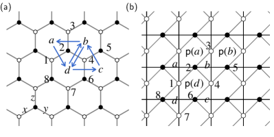
Figure 1: (a) Honeycomb lattice of the Kitaev model. The $x$-, $y$- and $z$-links are labeled respectively. The visons are located at the centre of hexagons, e.g., $a$, $b$, $c$ and $d$ highlighted in the schematic. $A$/$B$-sublattice sites are represented by open/filled disks. (b) The tilted honeycomb lattice with vertices placed on the links of a square lattice. Visons are now located at the vertices of the square lattice, while the $\varepsilon$ fermions sit at plaquettes. $A$-sublattice sites of the original honeycomb lattice now all align on vertical links of the square lattice.

II Kitaev model Perturbed by a Zeeman field

The model of interest is the Kitaev honeycomb model with a Haldane mass term [1]:

$$H=H_{K}-\kappa\sum_{i,j,k}X_{i}Y_{j}Z_{k},$$ (1)

$$H_{K}=K\left(\sum_{x\text{-links}}X_{i}X_{j}+\sum_{y\text{-links}}Y_{i}Y_{j}+\sum_{z\text{-links}}Z_{i}Z_{j}\right).$$

Here $X_{i}$, $Y_{j}$, $Z_{k}$ are the Pauli matrices of spins residing in the sites of the honeycomb lattice (see Fig. 1(a)). The above Hamiltonian is exactly solvable, and features a dispersive band of itinerant Majorana fermions and a gapped flat band of visons with an energy $E_{0}\approx 0.15|K|$ for $|\kappa|\ll|K|$ [1]. The term $\kappa$ induces a Haldane mass on the Majorana fermions that would otherwise have a gapless dispersion (see Ref. [1] for the choice of $i,j,k$ in the summation). Therefore this term is needed in order to have a fully gapped topologically ordered state and exponentially localized Majorana zero modes carried by the vison. Throughout the paper we will keep $\kappa$ as an independent parameter of the model, but we will view it implicitly as a term that is perturbatively generated by a physical Zeeman field, whose leading form is $\kappa\approx h_{x}h_{y}h_{z}/K^{2}$ [1], and in particular in all of our subsequent discussion it is understood that we fix $\operatorname{sgn}(\kappa)=\operatorname{sgn}(h_{x}h_{z}h_{y})$. It should be noted that in the presence of other types of perturbations, the induced Haldane mass term can scale linearly with $h$ [47], therefore a finite $\kappa$ term is physically relevant in those cases as well.

In addition to the above, we include the following explicit Zeeman coupling to $H$ in Eq. (1):

$$\Delta H=-\sum_{j}(h_{x}X_{j}+h_{y}Y_{j}+h_{z}Z_{j}).$$ (2)

The above term is produced by an external magnetic field. Crucially, this term induces not only the aforementioned Haldane mass term (provided that each component of the magnetic field is non-zero), but also the motion and pair creation/annihilation of the vison particles, destroying the exact solvability of the model. We will therefore treat this term as a perturbation. Our goal is to compute the perturbative hoppings and band dispersions that that this term induces on the visons, and to compute the real space phases that result from such vison motion when it is transported around a unit cell of its triangular lattice. While the magnitude of these hoppings will depend on the detailed form of the perturbation that induces the vison hopping, we wish to emphasize that this phase is independent on the specific detailed form of the operator that induces the vison motion, as long as it respects translational symmetry, since this phase is a universal property of the topologically ordered state enriched by translational symmetry, as recently argued in Ref. [38]. Therefore, as we will see, this phase is in exact agreement with the phase that was computed in Ref. [38] with a perturbation different from the Zeeman field.

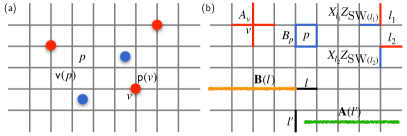
Figure 2: (a) Schematic of a real space configuration of the $e$ (red dots) and $\varepsilon$ (blue dots) particles. At each vertex $v$, there is a boson ($e$) mode with creation/annihilation operators $b_{v}^{\dagger}/b_{v}$. Within each plaquette $p$, there is a complex fermion ($\varepsilon$) mode with creation/annihilation operator $c_{p}^{\dagger}/c_{p}$, which is equivalent to two Majorana modes $\gamma_{p}$ and $\gamma^{\prime}_{p}$. (b) Spin operators and paths involved in the duality mapping. The Pauli $X$ ($Z$) matrices at a link is represented by a red (blue) colored bond covering the link. For a vertical/horizontal link $l_{1/2}$, $\text{SW}(l_{1/2})$ is the horizontal/vertical link to its southwest which connects to it. The path $\mathbf{B}(l)$ (orange thick line) contains all the vertices to the left of a horizontal link $l$ and the dual lattice path $\mathbf{A}(l^{\prime})$ (green thick line) contains all the plaquettes to the right of a vertical link $l^{\prime}$.

III Methods

III.1 Vison hoppings in the honeycomb lattice

The visons can be viewed as being located at the center of each hexagon. The vison parity operator at a hexagon/plaquette $p$, $W_{p}$ equals $-1\ (1)$ when a vison is present (absent) in a plaquette, and it is a product of the Pauli matrices of the $6$ spins surrounding $p$ [1]. For example, for the hexagon $d$ in Fig. 1(a), we have

$$W_{d}=X_{4}Y_{6}Z_{7}X_{8}Y_{1}Z_{2}.$$ (3)

For $H$ in Eq. (1), the vison parity $W_{p}$ is a constant of motion. However, its value ($\pm 1$) can be flipped by local spin operators. For example, for an $\alpha$-link ($\alpha=X,Y,Z$) between vertices $i$ and $j$, $\alpha_{i}$ and $\alpha_{j}$ anti-commute with vison parities at both plaquettes sandwiching the link $(i,j)$, and commute with the vison parities at other hexagons. Therefore, $\alpha_{i/j}$ can induce vison hoppings across the link $(i,j)$. The Zeeman coupling $\Delta H$ in Eq. (2) involves a sum of all the local spin operators, as a result, it can also induce vison hopping across each link. Below we will illustrate how to extract the vison hopping amplitudes, induced by $\Delta H$, from an example.

Let us consider an eigenstate of $H$ from Eq. (1) consisting of two far distant visons. We are interested in the “single-particle” properties of the visons, therefore, we will take one of these visons simply as an auxiliary vison that is held immobile while the other is allowed to move (this can be accomplised by only acting with the perturbation $\Delta H$ from Eq. (2) within the region containing the mobile vison of interest). We place the immobile vison at a hexagon at $\mathbf{R}_{0}$, and consider fluctuations of the mobile vison within the hexagon $a$, $b$, $c$ or $d$ in Fig. 1(a). The lowest energy eigenstate of $H$ for each two-vison configuration is denoted as $|\Phi(\mathbf{R}_{0},\mathbf{R}_{l})\rangle$, with $l{\,=\,}a,b,c,d$. In the limit in which both visons are much farther than the typical localization length of their Majorana zero modes, these four states will be degenerate. Moreover, when $\kappa$ is finite, there will be a gap to all excitations and therefore only these configurations that differ by changing the position of the vison will be connected by the perturbation $\Delta H$. Under these conditions one can then conceptualize these processes as coherent hopping of the vison particles. Then the leading in $\Delta H$ perturbative hopping amplitude of the vison from $d$ to $b$ (due to $\Delta H$) is given by

$$t_{b,d}\equiv\langle\Phi(\mathbf{R}_{0},\mathbf{R}_{b})|\Delta H|\Phi(\mathbf{R}_{0},\mathbf{R}_{d})\rangle.$$ (4)

From the definition of vison parity operator discussed above, one can see that only $Y_{2}$ and $Y_{4}$ anticommute with $W_{d}$ and $W_{b}$ while commuting with vison parities at all other hexagons. Therefore,

$$t_{b,d}=-h_{y}\langle\Phi(\mathbf{R}_{0},\mathbf{R}_{b})|Y_{2}+Y_{4}|\Phi(\mathbf{R}_{0},\mathbf{R}_{d})\rangle.$$ (5)

Similarly, it is straightforward to show the following expressions for the other hoppings:

$$t_{a,b}=-h_{z}\langle\Phi(\mathbf{R}_{0},\mathbf{R}_{a})|Z_{3}+Z_{2}|\Phi(\mathbf{R}_{0},\mathbf{R}_{b})\rangle,$$ (6a)

$$t_{b,c}=-h_{x}\langle\Phi(\mathbf{R}_{0},\mathbf{R}_{b})|X_{4}+X_{5}|\Phi(\mathbf{R}_{0},\mathbf{R}_{c})\rangle.$$ (6b)

Once the effective vison hopping for each link is obtained, one can extract the vison Berry phase acquired in a closed hopping associated with each closed path. For example, the phase acquired by hopping in the triangle $d\rightarrow b\rightarrow a\rightarrow d$ is defined as:

$$\phi_{abd}=\operatorname{Im}\ln(t_{d,a}t_{a,b}t_{b,d}),$$ (7)

and the phase acquired by hopping on the unit cell of translations $d\rightarrow c\rightarrow b\rightarrow a\rightarrow d$ is:

$$\phi_{abcd}=\operatorname{Im}\ln(t_{d,a}t_{a,b}t_{b,c}t_{c,d}).$$ (8)

If the phase $\phi_{abcd}$ aquired around a unit cell of the microscopic translational symmetries is not $0\pmod{2\pi}$, then the translations have a projective implementation on the vison particle [48, 49]. As discussed in Refs. [50, 41, 38] for topologically ordered states with deconfined $Z_{2}$ gauge fields, this phase is expected to be either $0$ or $\pi$ and its value is a robust topological characteristic of the phase as long as the the microscopic translational symmetry of the model is enforced. Notice, however, that these considerations do not apply to the phase $\phi_{abd}$ acquired around a single triangle, because this motion cannot be generated by the elements of the microscopic translation group, and therefore this phase can be sensitive to perturbations when only the translational symmetry is enforced.

The above formulae then define the mathematical problem at hand. The problem of computing these overlaps has been recently addressed in Ref. [37] employing the parton representation of spins. In the next section, we will however employ a different method that relies in an exact lattice duality developed in Ref. [38] building on the previous work of Refs. [39, 41].

III.2 Vison hoppings from the duality mapping

To use the duality mapping of Ref. [38], it is convenient to change the usual basis of the Kitaev model by performing a unitary transformation $U$. The transformation $U$ only affect the spins from $A$-sublattice sites (see Fig. 1(a)):

$$X_{j}\leftrightarrow Z_{j},\ Y_{j}\rightarrow-Y_{j},\quad\forall j\in A.$$ (9)

The spin Hamiltonians in Eq. (1) and Eq. (2) will be transformed accordingly, i.e., $H_{K}\rightarrow UH_{K}U^{-1}=\tilde{H}_{K}$, $\Delta H\rightarrow U\Delta HU^{-1}=\Delta\tilde{H}$:

$$\tilde{H}_{K}= K\left(\sum_{\begin{subarray}{c}x\text{-link},\\ i\in A\end{subarray}}Z_{i}X_{j}-\sum_{\begin{subarray}{c}y\text{-link},\\ i\in A\end{subarray}}Y_{i}Y_{j}+\sum_{\begin{subarray}{c}z\text{-link},\\ i\in A\end{subarray}}X_{i}Z_{j}\right),$$

$$\Delta\tilde{H}= -\sum_{i\in A}(h_{z}X_{i}-h_{y}Y_{i}+h_{x}Z_{i})$$

$$-\sum_{j\in B}(h_{x}X_{j}+h_{y}Y_{j}+h_{z}Z_{j}),$$ (10)

and similarly for the $\kappa$ term. In this new basis the vison parity reads as:

$$W_{d}\rightarrow\tilde{W}_{d} =Z_{4}Y_{6}X_{7}X_{8}(-Y_{1})Z_{2}$$

$$=X_{6}X_{7}X_{8}X_{1}Z_{1}Z_{2}Z_{4}Z_{6}.$$ (11)

And therefore, by identifying the sites of the honeycomb lattice with the links of a square lattice as depicted in Fig. 1(b), this operator can be viewed as a product of the star ($A_{d}$) and plaquette ($B_{\mathsf{p}(d)}$) operators of the standard toric code model [51] (see Fig. 2(b)), as discussed in Refs. [39, 40, 41, 38].

We will review here the exact duality mapping introduced in Ref. [38] for the case of an infinite system, and refer the reader to Ref. [38] for details of the mapping on a finite open and periodic lattices. The lattice duality allows to map the tensor product Hilbert space of spins onto a tensor product Hilbert space of the “visons” and “spinons”. The vison is a spinless hard-core boson which can viewed as being located at the vertices of the square lattice (see Fig. 2(a)), analogous to the “$e$-particles” of the toric code. Therefore we assign vison hard-core boson creation/annihilation operators, $b_{v}^{\dagger}$, $b_{v}$, with every vertex “$v$”. The vison parity operator is then mapped as follows:

$$\tilde{W}_{v}\leftrightarrow e^{i\pi b_{v}^{\dagger}b_{v}}.$$ (12)

On the other hand the spinon degrees of freedom correspond to those of a single spinless complex fermion mode per unit cell (which can be viewed as a descending of the “$\varepsilon$-particle” of the toric code [39, 40, 41, 38]). Therefore we introduce two spinon Majorana fermion modes, $\gamma_{p},\gamma^{\prime}_{p}$ for every plaquette “$p$” of the lattice as depicted in Fig. 2(a). The fermion parity maps onto the following plaquette operator:

$$B_{\mathsf{p}(d)}=Z_{1}Z_{2}Z_{4}Z_{6}\leftrightarrow-i\gamma_{\mathsf{p}(d)}\gamma^{\prime}_{\mathsf{p}(d)}.$$ (13)

Here the operators $Z_{1}\cdots Z_{6}$ are those appearing in the usual plaquette term of the toric code, $\mathsf{p}(d)$ stands for the plaquette to the northeast of vertex $d$, as depicted in Fig. 1(b). We can combine the Majorana modes into complex fermion operators as follows:

$$c_{p}=(\gamma_{p}+i\gamma^{\prime}_{p})/2,\ c_{p}^{\dagger}=(\gamma_{p}-i\gamma^{\prime}_{p})/2.$$ (14)

Note that $-i\gamma_{p}\gamma^{\prime}_{p}{\,=\,}e^{i\pi c_{p}^{\dagger}c_{p}}$.

We will now present the “dictionary” that allows to map exactly any local operator acting the underlying physical spin degrees of freedom onto operators acting on the dual vison and spinon degrees of freedom, introduced in Ref. [38]. The mapping of spin operators on a link $l$ is the following:

1. Vertical $l$:

   $$Z_{l}\leftrightarrow(b_{v_{1}}+b_{v_{1}}^{\dagger})(b_{v_{2}}+b_{v_{2}}^{\dagger})e^{i\pi\alpha_{l}}$$ (15a)

   $$X_{l}Z_{\text{SW}(l)}\leftrightarrow i\gamma_{p_{1}}\gamma^{\prime}_{p_{2}}.$$ (15b)

2. Horizontal $l$:

   $$Z_{l}\leftrightarrow(b_{v_{1}}+b_{v_{1}}^{\dagger})(b_{v_{2}}+b_{v_{2}}^{\dagger})$$ (16a)

   $$X_{l}Z_{\text{SW}(l)}\leftrightarrow e^{i\pi\beta_{l}}i\gamma_{p_{1}}\gamma^{\prime}_{p_{2}}.$$ (16b)

Where:

$$\alpha_{l}=\sum_{p\in\mathbf{A}(l)}c_{p}^{\dagger}c_{p},\ \beta_{l}=\sum_{v\in\mathbf{B}(l)}b_{v}^{\dagger}b_{v}.$$ (17)

Here for a vertical (horizontal) link $l$, $v_{1}$ and $v_{2}$ are the two vertices connected by it, while $p_{1}$ and $p_{2}$ are the two plaquettes at the left and right (top and bottom) sides of it, $\text{SW}(l)$ is the link to the southwest of $l$ which also connects to it (see Fig. 2(b)). Also $\mathbf{A}(l)$ ($\mathbf{B}(l)$) denotes sets of plaquettes (vertices) that reside on a string in the dual (direct) lattice and are depicted in Fig. 2(b). These “string” operators are the ones encoding that the vison and the spinon have a non-local statistical interactions that makes them behave as mutual semions. Notice that the spin operators described above form a complete algebraic basis out of which any other operator can be obtained by taking sums, products and multiplication by complex numbers, from this basis.

In particular, we can apply the above dictionary to re-write the Hamiltonian from Eq. (III.2) in terms of vison and spinon degrees of freedom, leading to:

$$\tilde{H}= K\sum_{p}\left[e^{i\pi\beta_{\tilde{L}(p,p+\hat{y})}}(i\gamma_{p+\hat{y}}\gamma^{\prime}_{p}+i\gamma_{p+\hat{y}}\gamma^{\prime}_{p+\hat{x}})+i\gamma_{p}\gamma^{\prime}_{p+\hat{x}}\right]$$

$$-\kappa\sum_{p}\left[e^{i\pi\beta_{\tilde{L}(p,p+\hat{y})}}(i\gamma_{p+\hat{y}}\gamma_{p-\hat{{x}}})+e^{i\pi b_{\mathsf{v}(p)}^{\dagger}b_{\mathsf{v}(p)}}(i\gamma_{p-\hat{x}}\gamma_{p})+e^{i\pi\beta_{\tilde{L}(p,p+\hat{y})}}(i\gamma_{p}\gamma_{p+\hat{y}})\right.$$

$$\left.+e^{i\pi\beta_{\tilde{L}(p-\hat{x},p-\hat{x}+\hat{y})}}(i\gamma^{\prime}_{p+\hat{y}}\gamma^{\prime}_{p})+i\gamma^{\prime}_{p+\hat{x}}\gamma^{\prime}_{p}+e^{i\pi\beta_{\tilde{L}(p,p-\hat{y})}}(i\gamma^{\prime}_{p-\hat{y}}\gamma^{\prime}_{p+\hat{x}})\right].$$ (18)

Here $\mathsf{v}(p)$ denotes the vertex to the southwest of plaquette $p$ (see Fig. 2(a)), $\tilde{L}(p,p^{\prime})$ stands for the link sandwiched by plaquettes $p$ and $p^{\prime}$. Notice that the above Hamiltonian explicitily commutes with the vison occupation of all the vertices in the lattice and the remaining dynamical degrees freedom are described by a fermion bilinear model, as expected.

On the other hand, one can show that the $\Delta\tilde{H}$ in Eq. (III.2) can be re-written as:

$$\Delta\tilde{H}= -\sum_{v}\left[h_{z}(b_{v}+b_{v}^{\dagger})(b_{v+\hat{x}}+b_{v+\hat{x}}^{\dagger})(1+i\gamma_{\mathsf{p}(v)}\gamma^{\prime}_{\mathsf{p}(v)+\hat{x}})+h_{y}(b_{v-\hat{x}}+b_{v-\hat{x}}^{\dagger})(b_{v+\hat{y}}+b_{v+\hat{y}}^{\dagger})(\gamma_{\mathsf{p}(v)-\hat{x}}\gamma^{\prime}_{\mathsf{p}(v)})e^{i\pi\alpha_{L(v,v+\hat{y})}}\right.$$

$$+h_{y}e^{i\pi\beta_{L(v+\hat{y},v+\hat{y}+\hat{x})}}(b_{v}+b_{v}^{\dagger})(b_{v+\hat{x}+\hat{y}}+b_{v+\hat{x}+\hat{y}}^{\dagger})(-\gamma_{\mathsf{p}(v)+\hat{y}}\gamma^{\prime}_{\mathsf{p}(v)})e^{i\pi\alpha_{L(v,v+\hat{y})}}$$

$$\left.+h_{x}\left(e^{i\pi\beta_{L(v+\hat{y},v+\hat{y}+\hat{x})}}i\gamma_{\mathsf{p}(v)+\hat{y}}\gamma^{\prime}_{\mathsf{p}(v)}+1\right)(b_{v}+b_{v}^{\dagger})(b_{v+\hat{y}}+b_{v+\hat{y}}^{\dagger})e^{i\pi\alpha_{L(v,v+\hat{y})}}\right].$$ (19)

Here $L(v,v^{\prime})$ stands for the link connecting vertices $v$ and $v^{\prime}$. As we see, the Zeeman term contains vison hopping and pair creation terms, creating an impediment to solving it exactly.

Therefore our strategy is to treat $\Delta\tilde{H}$ as a perturbation acting on the exact eigenstates of Eq. (III.2). Let us discuss how to uniquely label these states. An eigenstate of Eq. (III.2) with $N$ visons placed in the vertices $\{v_{1},....,v_{N}\}$, can be written as a tensor product of vison and spinon degrees of freedom as follows:

$$b_{v_{1}}^{\dagger}\dots b_{v_{N}}^{\dagger}|0\rangle\otimes|\Psi^{\varepsilon}(\mathbf{R}_{1},\dots,\mathbf{R}_{N})\rangle,$$ (20)

where $\mathbf{R}_{i}$ denotes the position of vertex $v_{i}$. The first term specifies the vison locations and the second term is the fermionic spinon wavefunction resulting from diagonalizing the effective BdG Hamiltonian $H^{\varepsilon}(\mathbf{R}_{1},\dots,\mathbf{R}_{N})$ associated with Eq. (III.2). Notice that this Hamiltonian has already a unique specified gauge choice for the vector potential that captures the long-range statistical interaction after the vison occupations are given and viewed as constants. We caution that the tensor product structure above is in a dual Hilbert space and does not have a simple relation to the tensor structure of the underlying physical spin degrees of freedom (see Ref. [38] for further discussions).

Let us now specialize to the case of two visons to compute the matrix elements described in Eqs. 4, 5 and 6. These vison hopping elements can then systematically computed. For example the hopping between vertices $a$ and $b$ (see Fig. 1(b)) can be obtained as follows:

$$t_{a,b}= -h_{z}\langle 0|b_{0}b_{a}\otimes\langle\Psi^{\varepsilon}_{0}(\mathbf{R}_{a},\mathbf{R}_{0})|(b_{a}+b_{a}^{\dagger})(b_{b}+b_{b}^{\dagger})$$

$$(1+i\gamma_{\mathsf{p}(a)}\gamma^{\prime}_{\mathsf{p}(b)})\ b_{b}^{\dagger}b_{0}^{\dagger}|0\rangle\otimes|\Psi^{\varepsilon}_{0}(\mathbf{R}_{b},\mathbf{R}_{0})\rangle$$

$$= -h_{z}\langle\Psi^{\varepsilon}_{0}(\mathbf{R}_{a},\mathbf{R}_{0})|(1+i\gamma_{\mathsf{p}(a)}\gamma^{\prime}_{\mathsf{p}(b)})|\Psi^{\varepsilon}_{0}(\mathbf{R}_{b},\mathbf{R}_{0})\rangle.$$ (21)

Here $|\Psi^{\varepsilon}_{0}(\mathbf{R}_{j},\mathbf{R}_{0})\rangle$ is the lowest energy eigenstate of $H^{\varepsilon}(\mathbf{R}_{j},\mathbf{R}_{0})$. Similarly, the hopping between vertices $a$ and $d$ reads:

$$t_{d,a}= -h_{x}\langle\Psi^{\varepsilon}(\mathbf{R}_{d},\mathbf{R}_{0})|(1+i\gamma_{\mathsf{p}(a)}\gamma^{\prime}_{\mathsf{p}(d)})e^{i\pi\alpha_{L(a,d)}}$$

$$|\Psi^{\varepsilon}(\mathbf{R}_{a},\mathbf{R}_{0})\rangle.$$ (22)

Here $e^{i\alpha_{L(a,d)}}$ reflects the statistical interaction between visons and spinons, and we have assumed that the vertex $0$ is in the same row as vertex $d$.

We would like to briefly comment on the duality mapping for the case of a periodic system, which is the geometry that we use for the numerical implementation to be described in the next section. There are two global constraints on a torus:

$$\prod_{v}\tilde{W}_{v}=1,\ \prod_{p}B_{p}=1.$$ (23)

Therefore only states with an even number of visons and spinons are physical in the torus. Moreover, there are additionally two global Wilson loop degrees of freedom associated with the non-contractible loops around the torus. For the exactly solvable model where the visons are static, the topological degrees of freedom associated with the Wilson loops can be taken to be two quantum numbers with values $z_{1,2}=\pm 1$ that specify whether the spinons have periodic or anti-periodic boundary conditions along the $x$- or $y$-directions of the torus respectively. Therefore the fermionic BdG eigenstates are labeled as: $|\Psi^{\varepsilon}_{0}(\mathbf{R}_{j},\mathbf{R}_{0};z_{1},z_{2})\rangle$. The vison hoppings can then be calculated in the same way as shown in Sections III.2 and III.2. More details on the duality mapping on a torus can be found in Ref. [38].

In the next section, we will discuss the results with $(z_{1},z_{2}){\,=\,}(-1,-1)$, i.e., anti-periodic boundary conditions (APBC) for $\varepsilon$ particles. The results with periodic boundary condition (PBC) ($(z_{1},z_{2})=(1,1)$) are presented in Appendix A.

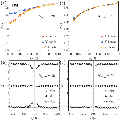
Figure 3: The vison hopping amplitude and Berry phases with FM coupling. (a) Hopping amplitudes with system size $N_{\text{row}}{\,=\,}20$. (b) The Berry phases associated with two minimal triangles and the plaquette path. (c-d) Same quantities for $N_{\text{row}}{\,=\,}50$. The magnitude of the hopping is independent of $\operatorname{sgn}(\kappa)=\operatorname{sgn}(h_{x}h_{z}h_{y})$, therefore we only present results for positive $\kappa$. The amplitudes have been normalized for a Zeeman field along the $[111]$ direction: $h_{x}{\,=\,}h_{y}{\,=\,}h_{z}{\,=\,}h/\sqrt{3}$, but the hoppings for other directions of the Zeeman field can be easily estimated from the above plots by re-scaling using Eqs. (5)-(8).

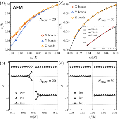
Figure 4: The vison hopping amplitude and Berry phases with AFM coupling. (a) The hopping amplitude with system size $N_{\text{row}}{\,=\,}20$. (b) The Berry phases associated with two minimal triangles and the plaquette. (c-d) Same quantities for $N_{\text{row}}{\,=\,}50$. The inset of (c) is a log-log plot of the same data, which suggests $|t_{\alpha}|\approx 0.55|h_{\alpha}|\ |\kappa/K|^{\nu}$ with $\nu\approx 0.5$, when the vison hops across an $\alpha$-bond $\alpha\in\{X,Y,Z\}$ (see Fig. 1). Notice that the vison phases on the triangles depend on $\operatorname{sgn}(\kappa)=\operatorname{sgn}(h_{x}h_{z}h_{y})$. We use same the conventions for phases and for normalizing hoppings as in Fig. 3.

IV Vison hoppings and Berry phases

IV.1 Results for FM and AFM couplings

As the expressions in Sections III.2 and III.2 illustrate, the calculation of the vison hopping amplitudes and Berry phases has been reduced to a problem of computing matrix elements of operators between free fermion BCS ground states. The mathematical details on how to compute these matrix elements have been discussed in Refs. [52, 38], and we will here present results following the same approach of Ref. [38]. All the numerical results that we will show have been done for the square torus: $N_{\text{row}}{\,=\,}N_{\text{col}}$. For the plots that we will present we have taken the Zeeman field along the $[111]$ direction, so that $h_{x}{\,=\,}h_{y}{\,=\,}h_{z}{\,=\,}h/\sqrt{3}$. Nevertheless, the vison hoppings for other directions of the Zeeman field can be easily estimated from the Figs. 3 and 4 via a re-scaling using Eqs. 5, 6, 7 and 8 and keeping track of the corresponding change of $\kappa\approx h_{x}h_{y}h_{z}/K^{2}$.

Fig. 3 shows the results for the FM Kitaev model at two different system sizes: $N_{\text{row}}{\,=\,}20$ in (a-b), $N_{\text{row}}{\,=\,}50$ in (c-d). The hoppings are labeled according to the type of bonds crossed by the vison, e.g., $t_{a,b}\in Z$-bonds, $t_{b,d}\in Y$-bonds, $t_{d,a}\in X$-bonds (see Fig. 1(a)). Our results are consistent with the expected symmetry of the honeycomb lattice according to which the magnitudes of the hopping amplitude on all bonds are the same in the thermodynamic limit ($N_{\text{row}}\rightarrow\infty$), however the convergence degrades and becomes slower as the fermion gap vanishes for $\kappa\rightarrow 0$, as evidenced by contrasting the behavior of $N_{\text{row}}{\,=\,}20$ with $N_{\text{row}}{\,=\,}50$ in Fig. 3, and as further discussed in Appendix B . Moreover, we have observed that for strict $\kappa{\,=\,}0$ the vison hoppings are sensitive to the choice of fermion boundary conditions (Wilson loop sectors $(z_{1},z_{2})$), further indicating that the vison hopping may not be well defined in the $\kappa{\,=\,}0$ case (see Appendix A for more details). The horizontal dashed lines in Fig. 3(a) and (c) indicate the result of Ref. [37] for the magnitude of the hopping, which performed all calculations strictly at $\kappa{\,=\,}0$. We see that our extrapolation to $\kappa\rightarrow 0$ at $N_{\text{row}}{\,=\,}50$ (dashed curve in Fig. 3(c)) is in agreement with Ref. [37], and is given by $|t_{\alpha}|\sim 0.38|h_{\alpha}|$, when the vison hops across an $\alpha$-bond $\alpha\in\{X,Y,Z\}$ (see Fig. 1).

The phases for the FM model are shown in Fig. 3(b) and (d), for a vison hopping around an upper triangle $\phi_{\text{UT}}$ ($d\rightarrow b\rightarrow a\rightarrow d$ in Fig. 1), a lower triangle $\phi_{\text{LT}}$ ($d\rightarrow c\rightarrow b\rightarrow d$ in Fig. 1), and a Bravais unit cell $\phi_{\text{UC}}$ ($d\rightarrow c\rightarrow b\rightarrow a\rightarrow d$ in Fig. 1). We see clear evidence that for $\kappa\neq 0$ these phases approach the following values in the thermodynamic limit:

$$\phi_{\text{LT}} =-\phi_{\text{UT}}=\pi\operatorname{sgn}(\kappa)=\pi,\ {\rm(FM)}$$ (24a)

$$\phi_{\text{UC}} =0,\ {\rm(FM)}$$ (24b)

where in the last equality of Eq. (24a) we have used the fact that phases are defined modulo $2\pi$. The above is one of our central findings: the vison in the FM model acquires zero phase around a unit cell of the Bravais lattice, and thus translations act in a non-projective fashion.

The results for the AFM coupling are shown in Fig. 4. Interestingly, we find that the hopping amplitude approaches $0$ as $\kappa\rightarrow 0$ in the thermodynamic limit, in agreement with Ref. [37]. Even more remarkably, for non-zero $\kappa$, our results are approaching the following values of the phases around triangles and the unit cell in the thermodynamic limit:

$$\phi_{\text{LT}} =\phi_{\text{UT}}=-\frac{\pi}{2}\operatorname{sgn}(\kappa),\ {\rm(AFM)}$$ (25a)

$$\phi_{\text{UC}} =\pi,\ {\rm(AFM)}$$ (25b)

Therefore we see that the vison has acquires phase $\pi$ when moving around a unit cell and therefore translations need to be implemented projectively. Similar to the FM case, in the AFM model at $\kappa{\,=\,}0$ we also observe strong sensitivity on the spinon boundary conditions and system sizes (see Appendix A for more details).

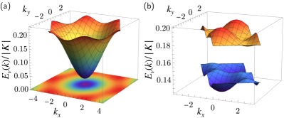
Figure 5: The vison bands for FM (a) and AFM (b) couplings at small Zeeman fields. The triangular lattice’s lattice constant is set to be $a{\,=\,}1$. (a) The bands for FM coupling with $h=0.1|K|$, so $\kappa/|K|{\,=\,}(h/\sqrt{3})^{3}/|K|^{3}\sim 10^{-4}$ according to perturbation theory [1]. The single vison excitation energy is found to be $E_{0}\approx 0.15|K|$. (b) The bands for AFM coupling with $\kappa/K=(h/\sqrt{3}K)^{3}=0.01$. For this $\kappa$ single vison excitation energy is $E_{0}\approx 0.16K$ (obtained for $N_{\text{row}}=30$). Note that for the FM Kitaev model, the vison band has a larger width and its band minumum is closer to zero.

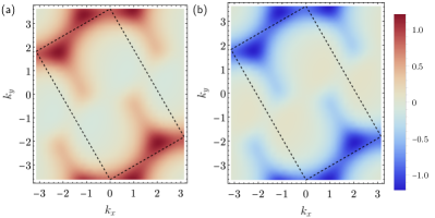
Figure 6: Berry curvature of the upper (a) and lower (b) vison bands in Fig. 5(b). The black dashed rectangle indicates the reduced Brillouin zone. The Chern number of the upper/lower band is $\pm 1$.

IV.2 Vison Chern bands

From the effective vison hoppings computed in the previous section we can construct the vison band dispersions for both FM and AFM couplings. For FM coupling, the vison does not experience flux within the unit cell ($\phi_{\text{UC}}{\,=\,}0$), and therefore, the vison band is simply that of a single-site nearest-neighbor tight-binding model in the triangular lattice. As a consequence this band has no Berry curvature. Fig. 5(a) shows the vison band dispersion at $h{\,=\,}0.1|K|$, $\kappa/|K|{\,=\,}(h/\sqrt{3}|K|)^{3}\sim 10^{-4}$, which has a small gap.

On the other hand, for the AFM model, $\phi_{\text{UT}}{\,=\,}\phi_{\text{LT}}{\,=\,}-\pi/2\operatorname{sgn}(\kappa)$ and $\phi_{\text{UC}}{\,=\,}\pi$. Therefore the vison unit cell needs to be doubled, giving rise to two vison bands. Fig. 5(b) shows the vison bands at $\kappa/K{\,=\,}(h/\sqrt{3}K)^{3}{\,=\,}0.01$. We have also calculated the Berry curvature and Chern number for each band. Interestingly, we found that both bands have a non-trivial topology, the higher/lower band has a Chern number $C{\,=\,}\pm 1$. The Berry curvatures for the two bands are shown in Fig. 6.

V Consistency check of vison phases via commuting projector Hamiltonians

In this section we would like to offer some supporting evidence that the phases that the vison acquires around a unit cell are indeed $0$ and $\pi$ for the FM and AFM Kitaev models, respectively. Currently we don’t know any method allowing us to compute these phases purely analytically when the fermionic Majorana spinons are forming a topological superconducting state with a non-zero BdG Chern number $C\neq 0$. Nevertheless, as argued in Ref. [41], when the Majorana spinons have zero Chern number ($C{\,=\,}0$), the phase that the vison acquires around each unit cell can indeed be computed analytically thanks to the fact that the state can be adiabatically deformed into the ground state of a Hamiltonian made out of sums of commuting projectors (like the toric code), and such adiabatic deformation can be performed without breaking the lattice translational symmetry of the model.

To exploit this idea, we will add a term to the Hamiltonian that drives a phase transition into a state with vanishing spinon Chern number ($C{\,=\,}0$) that can be described with commuting projector Hamiltonians. By following the discussion of Ref. [41], we will select this commuting projector state such that the vison still acquires the same phase around a unit cell as in the original state of interest with non-zero $C$. By explicitly verifying that the the phase of the vison around a plaquette indeed does not change across such a phase transition, we will be able to clearly confirm that the values of the vison phases that we have computed numerically agree with those of the simpler commuting projector Hamiltonian state.

But what are these ideal commuting projector states? As discussed in Refs. [41, 54, 55, 56], the gapped paired BCS states of fermionic spinons with translational symmetry can be classified by the Chern number $C\in\mathbb{Z}$ and by four parity indices $\zeta_{k}=\pm 1$, associated with the four special high-symmetry points (HSPs) of the Brillouin zone: $\{(0,0),(0,\pi),(\pi,0),(\pi,\pi)\}$. The value $\zeta_{k}=-1(1)$ is viewed as non-trivial (trivial), and it indicates that the ground state has an odd (even) number fermions occupying the special momentum $k$ state (if such a $k$ state is allowed by the boundary conditions and the size of the system). The Chern number and these parity indices are related as follows:

$$(-1)^{C}=\zeta_{(0,0)}\zeta_{(0,\pi)}\zeta_{(\pi,0)}\zeta_{(\pi,\pi)}.$$ (26)

The states with commuting projector Hamiltonians of our interest have $C{\,=\,}0$ and either all the parity indices taking the trivial value ($\zeta_{k}{\,=\,}1$) or all taking the non-trivial value ($\zeta_{k}{\,=\,}-1$) . Among these states the one with all the four parity indices trivial ($\zeta_{k}{\,=\,}1$) and $C{\,=\,}0$ is adiabatically connected to a trivial “atomic insulator” vacuum of fermionic spinons, namely the state of spinon is completely empty, which is essentially a toric code vacuum state, which we label TC-AI₀ . As discussed in Refs. [41, 38], this state is adiabatically equivalent to the ground state of the usual toric code, and the vison in this case is simply the usual $e$-particle, which clearly acquires $0$ phase when moving around a unit cell.

On the other hand, the states with $\zeta_{k}=-1$ for all the four HSPs, are adiabatically connected to another trivial “atomic insulator” state, with one $\epsilon$ spinon per unit cell, which is the analogue of a fully occupied toric code state, which we label TC-AI₁ . The ideal commuting projector Hamiltonians in this case is the toric code model but with the opposite sign for both the vertex and plaquette couplings, so that every plaquette contains an $\varepsilon$-particle [41, 40, 38]. It is straightforward to verify that the vison ($e$-particle) in this state will acquire a $\pi$-flux when encircling a unit cell, simply because each unit cell contains an $\varepsilon$-particle, which is a semion relative to the $e$-particles.

By following the ideas of Ref. [38], we will now show that the vison in the FM Kitaev model is expected indeed to have the same phases as in the trivial atomic insulator of spinons TC-AI₀, namely $\phi_{\text{UC}}{\,=\,}0$, whereas the vison of the AFM Kitaev model has the same phase as in the trivial atomic insulator TC-AI₁, i.e., $\phi_{\text{UC}}{\,=\,}\pi$. The $\varepsilon$-particle’s band dispersion (obtained from the number-conserving part of the $\varepsilon$-particle Hamiltonian) for $H$ with FM and AFM couplings are shown in Figs. 7(a) and (b) respectively. For FM coupling, $\epsilon(0,0){\,=\,}-6|K|$, $\epsilon(\pi,0){\,=\,}\epsilon(0,\pi){\,=\,}\epsilon(\pi,\pi){\,=\,}2|K|$, thus $\zeta_{(0,0)}{\,=\,}-1$ and $\zeta_{k}{\,=\,}+1$ for the rest HSPs. Its parity indices at four HSPs are closer to those of TC-AI₀ state, so we expect $\phi_{\text{UC}}{\,=\,}0$ . As for AFM coupling, the $\varepsilon$ band dispersion is simply opposite to that of the FM case. The parity indices $\zeta_{(0,0)}{\,=\,}1$ and $\zeta_{k}{\,=\,}-1$ at other HSPs, which is closer to that of TC-AI₁ state. Therefore we expect $\phi_{\text{UC}}{\,=\,}\pi$ from the arguments of Ref. [38].

We will now provide direct numerical evidence for the above expected values of $\phi_{\text{UC}}$ in FM and AFM Kitaev model. To do so we add the following additional term $H_{1}$ into $H$, which reads (after the unitary transformation $U$ introduced in Sec. III.2):

$$UH_{1}U^{-1}=\sum_{p}\frac{\mu_{\varepsilon}}{2}(\prod_{l\in\text{boundary}(p)}Z_{l}-1).$$ (27)

Here $p$ stands for a plaquette in the square lattice (see Fig. 1(b)). Under the duality mapping discussed in Sec. III.2 and in Ref. [38], the above term is mapped into $\sum_{p}-\mu_{\varepsilon}c_{p}^{\dagger}c_{p}$. Therefore, this term simply introduces a chemical potential to $\varepsilon$-particles and therefore, it naturally drives the ground state into the commuting projector limit of the TC-AI₀ state when $\mu_{\varepsilon}$ is sufficiently negative and into the one of the TC-AI₁ state when $\mu_{\varepsilon}$ is sufficiently positive. We calculated the phase that the vison acquires around a unit cell, $\phi_{\text{UC}}$ at different $\kappa$ and $\mu_{\varepsilon}$. Fig. 8 shows the result for $\kappa/|K|{\,=\,}0.1$ with both FM and AFM Kitaev couplings. For FM coupling (Figs. 8(a-b)), as $\mu_{\varepsilon}$ is tuned to the band edges, the vison hopping crossing $Y$-bonds decreases while the hoppings crossing $X$- and $Z$-bonds are approaching $\sim 0.7$. When $-6|K|\leq\mu_{\varepsilon}{\,\leq\,}2|K|$, $\zeta_{(0,0)}{\,=\,}-1$ and $\zeta_{k}{\,=\,}1$ for the other three HSPs, the parity indices’ configuration is closer to that of TC-AI₀ state. Indeed, the vison phase $\phi_{\text{UC}}$ is always $0$ in this regime. When $\mu_{\varepsilon}<-6|K|$, since the bare $\varepsilon$ band is empty ($\zeta_{k}{\,=\,}1$ at all four HSPs), the $\varepsilon$ ground state is adiabatically connected to the TC-AI₀ state and $\phi_{\text{UC}}{\,=\,}0$. Therefore, $\phi_{\text{UC}}$ does note change its value across this FM-Kitaev to TC-AI₀ transition. On the other hand, when $\mu_{\varepsilon}$ becomes larger than $2|K|$, $\phi_{\text{UC}}$ suddenly jumps to $\pi$. This can be understood from the fact that in this regime, $\zeta_{k}{\,=\,}-1$ for all HSPs and the $\varepsilon$ ground state is adiabatically connected to TC-AI₁, so $\phi_{\text{UC}}$ should take the same value as that of TC-AI₁ state. For AFM coupling (Fig. 8(c-d)), as $\mu_{\varepsilon}$ is tuned to the band edge, the vison hopping crossing $X$- and $Z$-bonds are close to $\sim 0.5|h|$ while the hopping across $Y$-bonds decreases. For $-2|K|\leq\mu_{\varepsilon}\leq 6|K|$, $\zeta_{(0,0)}{\,=\,}1$ while $\zeta_{k}$ at all the other three HSPs are $-1$, which is closer to that of TC-AI₁ state. Indeed, we found that $\phi_{\text{UC}}$ is always $\pi$ across the AFM-Kitaev to TC-AI₁ ($\mu_{\varepsilon}\geq 6|K|$) transition. On the other hand, when the $\varepsilon$ ground state enters the TC-AI₀ regime ($\mu_{\varepsilon}{\,<\,}-2|K|$), $\phi_{\text{UC}}$ jumps to $0$. Therefore, our results thus indicate that the vison phase $\phi_{\text{UC}}$ for FM (AFM) Kitaev coupling is indeed the same as that of the TC-AI₀ (TC-AI₁) state, as expected from the considerations of Ref. [38].

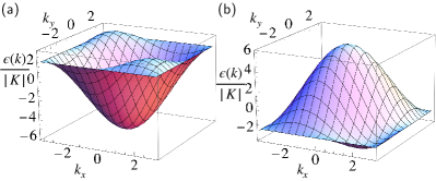
Figure 7: Number-conserving part of $\varepsilon$-particle bands (on a square lattice) from $\tilde{H}$ with FM (a) and AFM (b) couplings. The lattice constant is set to be $1$.

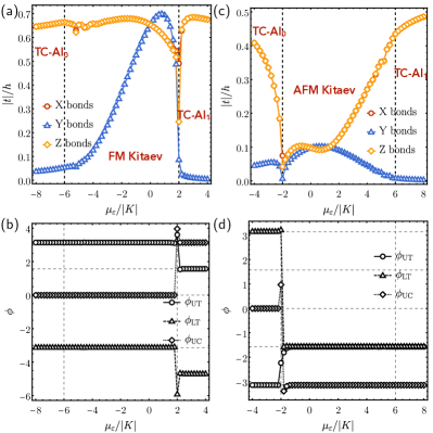
Figure 8: Vison hopping as a function of $\mu_{\varepsilon}$ at $\kappa/|K|$  = 0.1. (a-b) The hopping amplitude and $\phi$ for FM coupling. (c-d) Same quantities for AFM coupling. Calculations are done with $N_{\text{row}}=50$ and APBC.

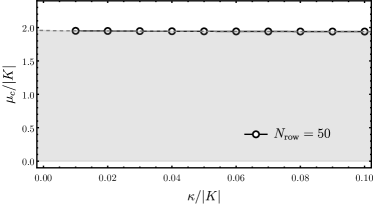
Figure 9: Critical $\mu_{c}$ for the $0$ to $\pi$ jump of $\phi_{\text{UC}}$ at different $\kappa$ with FM coupling. $N_{\text{row}}{\,=\,}50$. $\phi_{\text{UC}}{\,=\,}0$ in the gray region with a caveat that $\phi_{\text{UC}}$ at stricktly $\kappa{\,=\,}0$ could be ill-defined.

Moreover, we have performed same type of calculations at smaller $\kappa$ values, for each $\kappa$, we found a similar $0$ to $\pi$ jump behavior at some “critical” chemical potential $\mu_{c}$. Fig. 9 shows the result for $\mu_{c}$ at different $\kappa$ values with a FM coupling. It can be seen that $\mu_{c}$ is not sensitive to $\kappa$ at small $\kappa$ values, this can be understood from the perspective of our conjecture as $\kappa$ does not affect the number-conserving part (hopping and chemical potential) of $\varepsilon$ particles’ Hamiltonian, therefore $\zeta_{k}$ at all four HSPs are independent of $\kappa$. Below the $\mu_{c}$-$\kappa$ curve (the gray region in Fig. 9), there is always $\phi_{\text{UC}}{\,=\,}0$. Note that although the extrapolation of finite $\kappa$ results tends to suggest $\phi_{\text{UC}}{\,=\,}0$ for the $\kappa{\,=\,}0$ FM Kitaev model ($\mu_{\varepsilon}{\,=\,}0$), due to the reasons described previously, $\phi_{\text{UC}}$ at $\kappa{\,=\,}0$ may not be a well-defined quantity.

VI Summary and Discussion

Using a recently developed exact duality mapping [38] that allows to re-write the microscopic spin operators in terms of non-local visons and fermionic spinons degrees of freedom, we have investigated the nature of the motion of the emergent flux carrying vison particles in the Kitaev honeycomb model perturbed by a Zeeman field. This Zeeman field not only induces the well-known Haldane-type mass gap on the itinerant Majorana fermions, but also induces vison hopping, breaking the exact solvability of the model.

We have seen that while the FM ($K<0$) and the AFM ($K>0$) Kitaev models have the same Non-Abelian Ising topological order, they are sharply distinct phases of matter when viewed as topologically ordered states that are enriched by the discrete translational symmetry of the honeycomb lattice. As a consequence of this, the nature of the motion of the vison particle is sharply distinct in the FM vs the AFM Kitaev honeycomb models. For example, in the FM Kitaev model the vison acquires a trivial phase when it encircles around a unit cell of the honeycomb Bravais lattice: $\phi_{\text{UC}}{\,=\,}0$. Since there is a single vison site per unit cell (which can be viewed as located at the center of the plaquette), this implies that the vison moves effectively in a single-site triangular lattice with zero flux. There is, therefore, a single vison band which has zero Berry curvature and thus no associated intrinsic contribution the thermal Hall effect. To further back-up this conclusion, we have shown that the vison phase around the unit cell remains unchanged across a phase transition into another ground state that is adiabatically connected to the ground state of the standard toric code model, which is a commuting projector Hamiltonian where this phase can be computed fully analytically and where it is clear that translations act non-projectively on its anyon excitations.

On the other hand, in the AFM Kitaev model the vison acquires a non-trivial phase when it hops around a unit cell: $\phi_{\text{UC}}{\,=\,}\pi$. As a consequence lattice translations are implemented projectively on the vison, and the vison unit cell needs to be doubled. In this case, the vison has two separate bands with non-zero Chern numbers $C=\pm 1$, and an associated contribution to the intrinsic thermal Hall effect.

There are also crucial energetic differences to the vison bands in the FM vs AFM models. In the FM model, the magnitude of the vison hopping and band-width grow linearly with the Zeeman field, $|t_{\alpha}|\approx 0.38|h_{\alpha}|$, when the vison hops across an $\alpha$-bond ($\alpha=X,Y,Z$) (see Fig. 1) at the leading perturbative order, which agrees with the value reported in Ref. [37]. For the AFM model our results are consistent with a vanishing leading perturbative hopping of the vison that is linear in Zeeman fields, as also reported in Ref. [37]. However, we have seen that in the presence of the Haldane mass term of the Majorana fermions, $\kappa\approx h_{x}h_{y}h_{z}/K^{2}$ [1], the magnitude of the vison hopping becomes non-zero and scales as: $|t_{\alpha}|\propto|h_{\alpha}||\kappa/K|^{\nu}$ when the vison hops across an $\alpha$-bond $\alpha\in\{X,Y,Z\}$ (see Fig. 1), with $\nu\approx 0.5$ at small $\kappa$ and $h_{\alpha}$. As a consequence of this, the visons in the FM model are substantiallly more mobile at small values of the Zeeman field than in the AFM model. Therefore the Zeeman field is expected to destabilize more easily the FM Kitaev spin liquid via vison gap closing and condensation, relative to the AFM Kitaev spin liquid. This is naturally consistent with a variety of numerical studies which have reported that the FM Kitaev spin liquid is more fragile than the AFM Kitaev spin liquid against Zeeman field (see, e.g., Refs. [24, 25, 26, 27]). While the single-vison gap closing picture found here provides a natural mechanism for an instability of the Kitaev spin liquid, it should be noted that such a proliferation mechanism can also be applied to tightly bounded vison pairs. As discussed in Refs. [61, 62], a bounded vison pair also gains dynamics under perturbations like Zeeman field, Heisenberg and Gamma interactions. According to the magnitude of induced vison-pair hopping amplitudes of Refs. [61, 62], it was reported that the FM (AFM) Kitaev spin liquid is more robust (fragile) against Heisenberg interaction and fragile (robust) against Zeeman field and Gamma interaction, in agreement with our findings.

While the precise relation between the ideal spin liquids realized in the weakly perturbed Kitaev model that we have studied and the possible spin liquids observed in $\alpha$-RuCl₃ is currently far from clear, our study highlights the crucial importance of the sign of the Kitaev coupling $K$ in determining the universal properties of these states. While the larger share of studies devoted to determining this sign have advocated it to be ferromagnetic (see, e.g., Refs. [19, 20] for summaries), direct experimental inference of this sign has heavily relied in understanding the zig-zag AFM. However, in spite of being an ordered state, the zig-zag AFM state is in itself still a highly quantum fluctuating state that delicately depends on perturbations beyond the ideal Kitaev model [28, 29, 24, 25, 26, 27, 19, 20, 30, 31, 26]. One alternative state that is comparatively simpler to understand theoretically, but which however remains less experimentally explored, is the high-field polarized state. This state could offer a fresh alternative window to perform experiments that could more confidently cement our knowledge of the sign of this important coupling in $\alpha$-RuCl₃.

Finally, we would like to note that during the completion of our work an updated version of Ref. [37] appeared, and our results are in agreement with the various aspects where we overlap with that reference. The updated analysis of Ref. [37] was performed independently and largely in parallel to our work, and corrected an earlier version of that reference.

Appendix A Vison hoppings with periodic boundary conditions

In this section, we present the results of vison hoppings with $(z_{1},z_{2}){\,=\,}(1,1)$, i.e., PBC for $\varepsilon$ Majorana fermions. The vison hopping and Berry phases with FM and AFM couplings are shown in Figs. 10 and 12 respectively. At finite $\kappa$, the results are essentially the same as APBC results discussed in the main text. For comparison, we also present the APBC results at system size $N_{\text{row}}{\,=\,}10,\ 20$ with FM (Fig. 11) and AFM Kitaev coupling (Fig. 13).

The Zeeman field is aligned along the $[111]$ direction (same as in Sec. IV.1) and we present the results at $\kappa\geq 0$, the Berry phases are obtained with positive $h$. At finite $\kappa$, the vison hoppings and Berry phases are independent of the boundary conditions for both FM and AFM couplings (in the thermodynamic limit). The main difference is at $\kappa{\,=\,}0$. In the case with APBC, the results for the system sizes presented here seem to indicate $\phi_{\text{UC}}=0$ ($\pi$) for FM (AFM) couplings. On the other hand, with PBC, the vison hoppings crossing certain bonds could be very small, e.g., see the data in Fig. 10(a), Fig. 12(a) and (c). The smallness of the hopping across certain bonds creates an obstacle to unambiguously identify the vison hopping phases. For example, as shown in Fig. 12(a), because the vison hopping crossing certain bonds is close to zero, $\phi_{\text{UC}}$ jumps from $\pi$ to $0$ as $\kappa\rightarrow 0$. In Figs. 12(c-d), although $\phi_{\text{UC}}{\,=\,}\pi$ at $\kappa{\,=\,}0$, which looks consistent with the APBC result, we caution that such a $\phi_{\text{UC}}$ value is actually extracted from a numerically very small complex number (both the real and imaginary part being $\sim 10^{-20}$).

In summary, according to our calculation, while the vison hopping at a finite $\kappa$ is robust against spinon boundary conditions (Wilson loop sector), the vison hopping at $\kappa{\,=\,}0$ is very sensitive to the boundary conditions and system sizes. We believe this is due to the gapless nature for the $\kappa{\,=\,}0$ ($B$-phase) Kitaev model. Our results then clearly indicate that a small but non-zero $\kappa$ is needed to properly regularize the vison hopping phases in the fully gapped topologically ordered state.

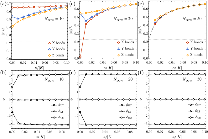
Figure 10: The vison hopping amplitude and $\phi$ with FM coupling at selected system sizes with PBC for the spinons. The results at finite $\kappa$ are consistent with APBC data presented in the main text, whereas at $\kappa{\,=\,}0$, the hoppings across certain bonds can be dropped to very small values at, which causes an ambiguity in determining the vison Berry phases.

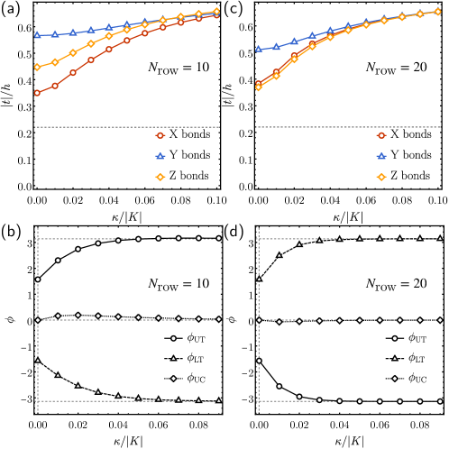
Figure 11: The vison hopping amplitude and $\phi$ with FM coupling at selected system sizes with APBC for the spinons.

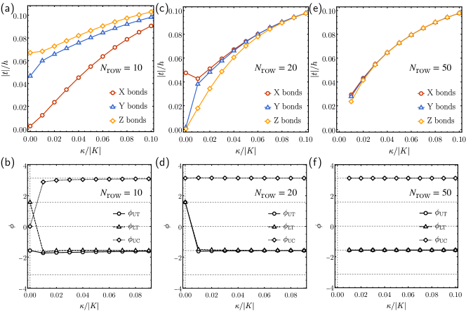
Figure 12: The vison hopping amplitude and $\phi$ with AFM coupling at selected system sizes with PBC for spinons.

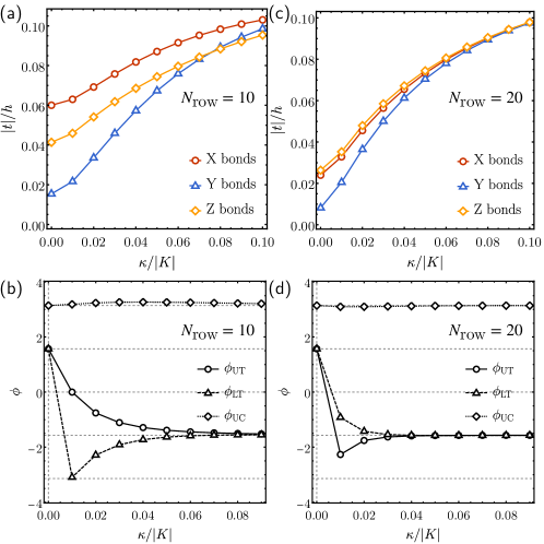
Figure 13: The vison hopping amplitude and $\phi$ with AFM coupling at selected system sizes with APBC for spinons.

Appendix B Finite-size scaling of vison hoppings and associated phases

Within our numerical calculation, the vison hoppings at finite $\kappa$ converges fast as the system size ($N_{\text{row}}\times N_{\text{row}}$) increases. Results at $\kappa{\,=\,}0.01|K|$ and $\kappa{\,=\,}0.02|K|$ with APBC are presented in Fig. 14. Results with FM coupling are shown in Fig. 14(a-b) and those with AFM coupling are shown in Fig. 14(c-d).

It was found that the convergence of vison hoppings with repect to $N_{\text{row}}$ is faster at larger $\kappa$ values. This also gives extra evidence of the strong sensitivity of the vison hoppings with system size in the case of strictly zero Haldane mass term $\kappa{\,=\,}0$.

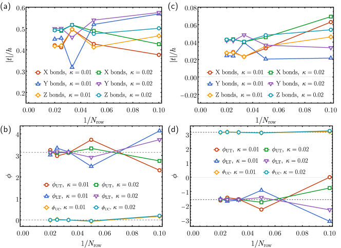
Figure 14: The scaling of vison hopping amplitudes and $\phi$ versus $1/N_{\text{row}}$. (a-b) results with $K{\,=\,}-1$; (c-d) results with $K{\,=\,}1$.

References

- Kitaev [2006] A. Kitaev, Anyons in an exactly solved model and beyond, Ann. Phys. 321, 2 (2006).
- Jackeli and Khaliullin [2009] G. Jackeli and G. Khaliullin, Mott insulators in the strong spin-orbit coupling limit: From heisenberg to a quantum compass and kitaev models, Phys. Rev. Lett. 102, 017205 (2009).
- Winter et al. [2017a] S. M. Winter, A. A. Tsirlin, M. Daghofer, J. van den Brink, Y. Singh, P. Gegenwart, and R. Valentí, Models and materials for generalized kitaev magnetism, Journal of Physics: Condensed Matter 29, 493002 (2017a).
- Takagi et al. [2019] H. Takagi, T. Takayama, G. Jackeli, G. Khaliullin, and S. E. Nagler, Concept and realization of kitaev quantum spin liquids, Nature Reviews Physics 1, 264 (2019).
- Johnson et al. [2015] R. D. Johnson, S. C. Williams, A. A. Haghighirad, J. Singleton, V. Zapf, P. Manuel, I. I. Mazin, Y. Li, H. O. Jeschke, R. Valentí, and R. Coldea, Monoclinic crystal structure of and the zigzag antiferromagnetic ground state, Phys. Rev. B 92, 235119 (2015).
- Cao et al. [2016] H. B. Cao, A. Banerjee, J.-Q. Yan, C. A. Bridges, M. D. Lumsden, D. G. Mandrus, D. A. Tennant, B. C. Chakoumakos, and S. E. Nagler, Low-temperature crystal and magnetic structure of , Phys. Rev. B 93, 134423 (2016).
- Banerjee et al. [2018] A. Banerjee, P. Lampen-Kelley, J. Knolle, C. Balz, A. A. Aczel, B. Winn, Y. Liu, D. Pajerowski, J. Yan, C. A. Bridges, A. T. Savici, B. C. Chakoumakos, M. D. Lumsden, D. A. Tennant, R. Moessner, D. G. Mandrus, and S. E. Nagler, Excitations in the field-induced quantum spin liquid state of -RuCl3, npj Quantum Materials 3, 1 (2018).
- Kasahara et al. [2018a] Y. Kasahara, K. Sugii, T. Ohnishi, M. Shimozawa, M. Yamashita, N. Kurita, H. Tanaka, J. Nasu, Y. Motome, T. Shibauchi, and Y. Matsuda, Unusual thermal hall effect in a kitaev spin liquid candidate , Phys. Rev. Lett. 120, 217205 (2018a).
- Banerjee et al. [2016] A. Banerjee, C. A. Bridges, J.-Q. Yan, A. A. Aczel, L. Li, M. B. Stone, G. E. Granroth, M. D. Lumsden, Y. Yiu, J. Knolle, S. Bhattacharjee, D. L. Kovrizhin, R. Moessner, D. A. Tennant, D. G. Mandrus, and S. E. Nagler, Proximate kitaev quantum spin liquid behaviour in a honeycomb magnet, Nat. Mater. 15, 733 (2016).
- Sandilands et al. [2015] L. J. Sandilands, Y. Tian, K. W. Plumb, Y.-J. Kim, and K. S. Burch, Scattering continuum and possible fractionalized excitations in , Phys. Rev. Lett. 114, 147201 (2015).
- Nasu et al. [2016] J. Nasu, J. Knolle, D. L. Kovrizhin, Y. Motome, and R. Moessner, Fermionic response from fractionalization in an insulating two-dimensional magnet, Nat. Phys. 12, 912 (2016).
- Yoshitake et al. [2016] J. Yoshitake, J. Nasu, and Y. Motome, Fractional spin fluctuations as a precursor of quantum spin liquids: Majorana dynamical mean-field study for the kitaev model, Phys. Rev. Lett. 117, 157203 (2016).
- Suetsugu et al. [2022] S. Suetsugu, Y. Ukai, M. Shimomura, M. Kamimura, T. Asaba, Y. Kasahara, N. Kurita, H. Tanaka, T. Shibauchi, J. Nasu, Y. Motome, and Y. Matsuda, Evidence for the first-order topological phase transition in a kitaev spin liquid candidate -rucl3, arXiv e-prints (2022), arXiv:2203.00275 [cond-mat.str-el] .
- Kasahara et al. [2018b] Y. Kasahara, T. Ohnishi, Y. Mizukami, O. Tanaka, S. Ma, K. Sugii, N. Kurita, H. Tanaka, J. Nasu, Y. Motome, T. Shibauchi, and Y. Matsuda, Majorana quantization and half-integer thermal quantum hall effect in a kitaev spin liquid, Nature 559, 227 (2018b).
- Yokoi et al. [2021] T. Yokoi, S. Ma, Y. Kasahara, S. Kasahara, T. Shibauchi, N. Kurita, H. Tanaka, J. Nasu, Y. Motome, C. Hickey, S. Trebst, and Y. Matsuda, Half-integer quantized anomalous thermal hall effect in the kitaev material candidate -rucl3, Science 373, 568 (2021).
- Bruin et al. [2022] J. A. N. Bruin, R. R. Claus, Y. Matsumoto, N. Kurita, H. Tanaka, and H. Takagi, Robustness of the thermal hall effect close to half-quantization in -RuCl3, Nat. Phys. 18, 401 (2022).
- Tanaka et al. [2022] O. Tanaka, Y. Mizukami, R. Harasawa, K. Hashimoto, K. Hwang, N. Kurita, H. Tanaka, S. Fujimoto, Y. Matsuda, E.-G. Moon, and T. Shibauchi, Thermodynamic evidence for a field-angle-dependent majorana gap in a kitaev spin liquid, Nat. Phys. 18, 429 (2022).
- Czajka et al. [2021] P. Czajka, T. Gao, M. Hirschberger, P. Lampen-Kelley, A. Banerjee, J. Yan, D. G. Mandrus, S. E. Nagler, and N. P. Ong, Oscillations of the thermal conductivity in the spin-liquid state of -RuCl 3, Nat. Phys. , 1 (2021).
- Laurell and Okamoto [2020] P. Laurell and S. Okamoto, Dynamical and thermal magnetic properties of the kitaev spin liquid candidate -RuCl3, npj Quantum Materials 5, 1 (2020).
- Maksimov and Chernyshev [2020] P. A. Maksimov and A. L. Chernyshev, Rethinking , Phys. Rev. Research 2, 033011 (2020).
- Sears et al. [2020] J. A. Sears, L. E. Chern, S. Kim, P. J. Bereciartua, S. Francoual, Y. B. Kim, and Y.-J. Kim, Ferromagnetic kitaev interaction and the origin of large magnetic anisotropy in -RuCl3, Nat. Phys. 16, 837 (2020).
- Chaloupka and Khaliullin [2016] J. c. v. Chaloupka and G. Khaliullin, Magnetic anisotropy in the kitaev model systems and , Phys. Rev. B 94, 064435 (2016).
- Suzuki et al. [2021] H. Suzuki, H. Liu, J. Bertinshaw, K. Ueda, H. Kim, S. Laha, D. Weber, Z. Yang, L. Wang, H. Takahashi, K. Fürsich, M. Minola, B. V. Lotsch, B. J. Kim, H. Yavaş, M. Daghofer, J. Chaloupka, G. Khaliullin, H. Gretarsson, and B. Keimer, Proximate ferromagnetic state in the kitaev model material -RuCl3, Nat. Commun. 12, 4512 (2021).
- Hickey and Trebst [2019] C. Hickey and S. Trebst, Emergence of a field-driven u(1) spin liquid in the kitaev honeycomb model, Nat. Commun. 10, 530 (2019).
- Zhu et al. [2018] Z. Zhu, I. Kimchi, D. N. Sheng, and L. Fu, Robust non-abelian spin liquid and a possible intermediate phase in the antiferromagnetic kitaev model with magnetic field, Phys. Rev. B 97, 241110 (2018).
- Gordon et al. [2019] J. S. Gordon, A. Catuneanu, E. S. Sørensen, and H.-Y. Kee, Theory of the field-revealed kitaev spin liquid, Nat. Commun. 10, 2470 (2019).
- Gohlke et al. [2018] M. Gohlke, R. Moessner, and F. Pollmann, Dynamical and topological properties of the kitaev model in a [111] magnetic field, Phys. Rev. B 98, 014418 (2018).
- Winter et al. [2017b] S. M. Winter, A. A. Tsirlin, M. Daghofer, J. van den Brink, Y. Singh, P. Gegenwart, and R. Valentí, Models and materials for generalized kitaev magnetism, Journal of Physics: Condensed Matter 29, 493002 (2017b).
- Rau and Kee [2014] J. G. Rau and H.-Y. Kee, Trigonal distortion in the honeycomb iridates: Proximity of zigzag and spiral phases in Na2IrO3, arXiv e-prints (2014), arXiv:1408.4811 [cond-mat.str-el] .
- Kim et al. [2015] H.-S. Kim, V. S. V., A. Catuneanu, and H.-Y. Kee, Kitaev magnetism in honeycomb with intermediate spin-orbit coupling, Phys. Rev. B 91, 241110 (2015).
- Sørensen et al. [2021] E. S. Sørensen, A. Catuneanu, J. S. Gordon, and H.-Y. Kee, Heart of entanglement: Chiral, nematic, and incommensurate phases in the kitaev-gamma ladder in a field, Phys. Rev. X 11, 011013 (2021).
- Read and Chakraborty [1989] N. Read and B. Chakraborty, Statistics of the excitations of the resonating-valence-bond state, Phys. Rev. B Condens. Matter 40, 7133 (1989).
- Kivelson [1989] S. Kivelson, Statistics of holons in the quantum hard-core dimer gas, Phys. Rev. B Condens. Matter 39, 259 (1989).
- Read and Sachdev [1991] N. Read and S. Sachdev, Large-N expansion for frustrated quantum antiferromagnets, Phys. Rev. Lett. 66, 1773 (1991).
- Senthil and Fisher [2000] T. Senthil and M. P. A. Fisher, Z2 gauge theory of electron fractionalization in strongly correlated systems, Phys. Rev. B Condens. Matter 62, 7850 (2000).
- Read and Green [2000] N. Read and D. Green, Paired states of fermions in two dimensions with breaking of parity and time-reversal symmetries and the fractional quantum hall effect, Phys. Rev. B 61, 10267 (2000).
- Joy and Rosch [2021] A. P. Joy and A. Rosch, Dynamics of visons and thermal Hall effect in perturbed Kitaev models, arXiv e-prints , arXiv:2109.00250 (2021), arXiv:2109.00250 [cond-mat.str-el] .
- Chen et al. [2022] C. Chen, P. Rao, and I. Sodemann, Berry Phases of Vison Transport in Topological Ordered States from Exact Fermion-Flux Lattice Dualities, arXiv e-prints , arXiv:2202.01238 (2022), arXiv:2202.01238 [cond-mat.str-el] .
- Chen et al. [2018] Y.-A. Chen, A. Kapustin, and Đ. Radičević, Exact bosonization in two spatial dimensions and a new class of lattice gauge theories, Ann. Phys. 393, 234 (2018).
- Pozo et al. [2021] O. Pozo, P. Rao, C. Chen, and I. Sodemann, Anatomy of Z2 fluxes in anyon fermi liquids and bose condensates, Phys. Rev. B 103, 035145 (2021).
- Rao and Sodemann [2021] P. Rao and I. Sodemann, Theory of weak symmetry breaking of translations in Z2 topologically ordered states and its relation to topological superconductivity from an exact lattice Z2 charge-flux attachment, Phys. Rev. Research 3, 023120 (2021).
- Kapustin and Fidkowski [2020] A. Kapustin and L. Fidkowski, Local commuting projector hamiltonians and the quantum hall effect, Commun. Math. Phys. 373, 763 (2020).
- Baskaran et al. [2007] G. Baskaran, S. Mandal, and R. Shankar, Exact results for spin dynamics and fractionalization in the kitaev model, Phys. Rev. Lett. 98, 247201 (2007).
- Tikhonov et al. [2011] K. S. Tikhonov, M. V. Feigel’man, and A. Y. Kitaev, Power-law spin correlations in a perturbed spin model on a honeycomb lattice, Phys. Rev. Lett. 106, 067203 (2011).
- Mandal et al. [2011] S. Mandal, S. Bhattacharjee, K. Sengupta, R. Shankar, and G. Baskaran, Confinement-deconfinement transition and spin correlations in a generalized kitaev model, Phys. Rev. B 84, 155121 (2011).
- Knolle et al. [2015] J. Knolle, D. L. Kovrizhin, J. T. Chalker, and R. Moessner, Dynamics of fractionalization in quantum spin liquids, Phys. Rev. B 92, 115127 (2015).
- Song et al. [2016] X.-Y. Song, Y.-Z. You, and L. Balents, Low-energy spin dynamics of the honeycomb spin liquid beyond the kitaev limit, Phys. Rev. Lett. 117, 037209 (2016).
- Wen [2002a] X.-G. Wen, Quantum orders and symmetric spin liquids, Phys. Rev. B 65, 165113 (2002a).
- Wen [2002b] X.-G. Wen, Quantum order: a quantum entanglement of many particles, Physics Letters A 300, 175 (2002b).
- Essin and Hermele [2013] A. M. Essin and M. Hermele, Classifying fractionalization: Symmetry classification of gapped spin liquids in two dimensions, Phys. Rev. B 87, 104406 (2013).
- Kitaev [2003] A. Y. Kitaev, Fault-tolerant quantum computation by anyons, Ann. Phys. 303, 2 (2003).
- Robledo [2009] L. M. Robledo, Sign of the overlap of hartree-fock-bogoliubov wave functions, Phys. Rev. C 79, 021302 (2009).
- Note [1] We only accessed for due to the slow convergence. This is why this point is missing for in Figs. 3(c-d).
- Kou and Wen [2009] S.-P. Kou and X.-G. Wen, Translation-symmetry-protected topological orders in quantum spin systems, Phys. Rev. B 80, 224406 (2009).
- Kou and Wen [2010] S.-P. Kou and X.-G. Wen, Translation-invariant topological superconductors on a lattice, Phys. Rev. B 82, 144501 (2010).
- Chiu et al. [2016] C.-K. Chiu, J. C. Y. Teo, A. P. Schnyder, and S. Ryu, Classification of topological quantum matter with symmetries, Rev. Mod. Phys. 88, 035005 (2016).
- Note [2] Those states with only two non-trivial and , are “weak topological superconductors”, namely stacks of lower dimensional superconductors. These states display “weak symmetry breaking” [41], and accordingly, the visons cannot be transported by local operators to all the nearest neighbor sites of the Bravais lattice.
- Note [3] This state is is also labeled as “AI0” in Ref. [41] and is labeled as “” in a recent general classification of the Abelian spin liquids (those with ) enriched by lattice translations [63].
- Note [4] This state is labeled as “AI1” in Ref. [41] and is labeled as “” in the recent general classification of the Abelian spin liquids enriched by lattice translations of Ref. [63].
- Note [5] We have conjectured in Ref. [38] that states with only one non-trivial parity index have , whereas states with non-trivial parity indices have . Our current numerics add further evidence to that conjecture.
- Zhang et al. [2021] S.-S. Zhang, G. B. Halász, W. Zhu, and C. D. Batista, Variational study of the kitaev-heisenberg-gamma model, Phys. Rev. B 104, 014411 (2021).
- Zhang et al. [2022] S.-S. Zhang, G. B. Halász, and C. D. Batista, Theory of the kitaev model in a [111] magnetic field, Nat. Commun. 13, 399 (2022).
- Song and Senthil [2022] X.-Y. Song and T. Senthil, Translation-enriched spin liquids and topological vison bands: Possible application to -RuCl3, arXiv e-prints (2022), arXiv:2206.14197 [cond-mat.str-el] .