PanScales showers for hadron collisions: all-order validation

Abstract

We carry out extensive tests of the next-to-leading logarithmic (NLL) accuracy of the PanScales parton showers, as introduced recently for colour-singlet production in hadron collisions. The tests include comparisons to (semi-)analytic NLL calculations of a wide range of hadron-collider observables: the colour-singlet boson transverse momentum distribution; global and non-global hadronic energy flow variables related to jet vetoes and analogues of jettiness distributions; (sub)jet multiplicities; and observables sensitive to the DGLAP evolution of the incoming momentum fractions. In the tests, we also include an implementation of a standard transverse-momentum ordered dipole shower, to establish the size of missing NLL effects in such showers, which, depending on the observable, can reach $100\%$. This paper, together with vanBeekveld:2022zhl , constitutes the first step towards process-independent NLL-accurate parton showers for hadronic collisions.

1 Introduction

Parton-shower simulations lie at the core of the majority of experimental and phenomenological studies in collider physics, accounting for the physics of parton branching across several orders of magnitude in momentum scale, independently of any specific observable. As such, one of the key questions, for both existing and new parton showers, is to understand and demonstrate their accuracy as compared to the standard QCD tool for multi-scale problems, namely logarithmic resummation. In a companion paper vanBeekveld:2022zhl , we recently formulated new classes of initial-state parton showers (PanGlobal and PanLocal) specifically designed to achieve next-to-leading logarithmic (NLL) accuracy in the context of hadron-hadron collisions. That paper included a number of tests of the kinematic recoil properties of the shower in the presence of two or three emissions, and validation against exact fixed-order matrix elements for spin and colour degrees of freedom. Those tests provided strong evidence that the new showers resolve key problems that are found in a standard Sjostrand:2006za ; Giele:2007di ; Schumann:2007mg ; Platzer:2009jq ; Hoche:2015sya ; Cabouat:2017rzi transverse-momentum ordered dipole approach, problems similar to those observed some time ago in final-state showers Hamilton:2020rcu and related to long-standing discussions about the treatment of initial-state recoil Nagy:2009vg ; Platzer:2009jq ; Hoche:2015sya ; Cabouat:2017rzi .

In this paper we present a number of all-order logarithmic tests in the context of colour-singlet production in proton–proton collisions. We test the new PanScales showers and, for the purpose of comparison, our implementation of a standard dipole shower, which we refer to as Dipole-$k_{t}$. These are the first all-order logarithmic tests to be carried out for initial-state showers, extending the developing body of recent work for final-state showers Dasgupta:2018nvj ; Dasgupta:2020fwr ; Hamilton:2020rcu ; Karlberg:2021kwr ; Hamilton:2021dyz . The tests serve two purposes. Firstly, they provide verification of the NLL accuracy for the PanScales showers across a wide range of observables, for an arbitrary number of emissions and taking into account all-order evolution of the strong coupling and the parton distribution functions (PDFs). Secondly, for showers that are not NLL accurate for a specific observable, they enable us to quantify the size of the deviation from the NLL result. While we will not go so far as to examine detailed phenomenological consequences in this paper, for each of the observables that we consider, we will comment on how it relates to widely discussed phenomenological questions.

We start our discussion with a brief review of the showers that we consider (Section 2) and then turn to a number of observables. One critical new test relative to the final-state case is the verification of the accuracy of PDF evolution (Section 3), and we comment briefly also on a practical observable that could be used for related measurements in data. We then consider a variety of global event quantities with distinct resummation structures. These include the jet-veto acceptance probability and observables related to 0-jettiness Stewart:2010tn (Section 4), for which the results are qualitatively similar (and in some cases quantitatively identical) to corresponding final-state tests. We then turn our attention to a particularly important global observable, the colour-singlet transverse momentum distribution (Section 5), for which we test not just the Sudakov region, but also the characteristic power-suppressed region identified long ago by Parisi and Petronzio Parisi:133268 . Then follow tests of energy flows in limited angular regions (Section 6), which play a role in many collider contexts, and a study of another basic observable, the average particle multiplicity (Section 7). We conclude with some exploratory phenomenological studies of the impact of our NLL showers on the $Z$-boson transverse momentum distribution and on the azimuthal correlations of jets (Section 8).

2 Brief overview of the showers and the testing approach

Throughout we consider the production of a colourless boson in proton–proton collisions, either $\bar{q}(\tilde{p}_{a})q(\tilde{p}_{b})\to Z$ or $g(\tilde{p}_{a})g(\tilde{p}_{b})\to H$, at a proton–proton centre-of-mass energy $\sqrt{s}$ and with Born invariant mass squared $m_{X}^{2}=(\tilde{p}_{a}+\tilde{p}_{b})^{2}$. The 4-momentum of the colour-singlet (hard system) is defined as

$$Q^{\mu}=m_{X}(\cosh y_{X},0,0,\sinh y_{X})\,,$$ (1)

where $X=Z,H$, and $y_{X}$ denotes the rapidity of the hard system. All partons are considered to be massless. We will compare the all-order behaviour of a standard dipole shower, which we refer to as Dipole-$k_{t}$, and the PanScales showers introduced in Ref. vanBeekveld:2022zhl suitable for hadron-hadron collisions. Here we give a brief summary of these showers, and full details can be found in Ref. vanBeekveld:2022zhl .

For all showers, the momentum of a newly emitted parton $k$ is decomposed as

$$p_{k}=a_{k}\tilde{p}_{i}+b_{k}\tilde{p}_{j}+k_{\perp},$$ (2)

where $\tilde{p}_{i,j}$ are the pre-branching momenta of the dipole constituents. By convention, $i$ labels the emitter and $j$ the spectator. The vector $k_{\perp}$ is space-like, orthogonal to $\tilde{p}_{i,j}$ and satisfies $k_{\perp}^{2}=-2a_{k}b_{k}\tilde{p}_{i}\cdot\tilde{p}_{j}$. The coefficients $a_{k}$ and $b_{k}$ are related to a shower-specific ordering variable $v$ and an auxiliary rapidity-like variable $\bar{\eta}$.

Dipole-$k_{t}$ showers:

our Dipole-$k_{t}$ class of showers follows in the long line of dipole showers inspired by Refs. Gustafson:1987rq ; Catani:1996vz ; Catani:2002hc . It shares substantial similarities with the dipole showers available in all the major Monte Carlo event generators, e.g. Pythia Cabouat:2017rzi , Sherpa Schumann:2007mg and Herwig Platzer:2009jq . In the soft-collinear limit, the ordering variable $v$ corresponds to the transverse momentum of the emission $|k_{\perp}|$.

The recoil scheme for emissions from final-final (FF) or final-initial (FI) dipoles is fully dipole-local, i.e.

$$p_{i} =a_{i}\tilde{p}_{i}+b_{i}\tilde{p}_{j}-k_{\perp}\,,$$ (3a)

$$p_{j} =b_{j}\tilde{p}_{j}\,,$$ (3b)

where the coefficients $a_{i},b_{i}$ and $b_{j}$ can be related to $a_{k}$ and $b_{k}$ using $p_{i,j}^{2}=0$ and $p_{i}\pm p_{j}+p_{k}=\tilde{p}_{i}\pm\tilde{p}_{j}$, taking the $+$ sign if the recoiler $j$ is in the final state, $-$ otherwise. For emissions from initial-initial (II) dipoles, the recoil is instead distributed globally, i.e.

$$p_{i}=a_{i}\tilde{p}_{i}\,,\qquad p_{j}=\tilde{p}_{j}\,,$$ (4)

followed by an event-wide boost (excluding the last emitted parton) that restores momentum conservation.

In the case of emissions from initial-final (IF) dipoles, where the initial-state parton is identified with the emitter, we consider two recoil schemes: one local and one global (see e.g. Refs. Platzer:2009jq ; Hoche:2015sya ), reflecting the variety of schemes implemented in public parton shower codes. In the fully local scheme, the transverse recoil is assigned to the final-state (spectator) parton, exactly like in the FI dipole. This implies that only II dipoles can impart transverse momentum recoil to the hard colour-singlet system. It is well-known that this leads to wrong predictions for the $Z$ transverse momentum distribution at the NLL-level Nagy:2009vg ; Platzer:2009jq ; Hoche:2015sya ; Cabouat:2017rzi , but it remains widely used, hence it will be of interest to quantify its deviation from the NLL expectation. In the global scheme, the recoil is distributed according to Eq. (3) (but with a positive sign for $k_{\perp}$). Next, all the particles in the event are boosted to realign $p_{i}$ with the beam axis. This effectively implies that the transverse recoil is redistributed across the event.

For any dipole type where the assignment of transverse recoil depends on which end of the dipole is the emitter, the choice of emitter is based on the end of the dipole that is closer in angle to the radiation in the dipole centre-of-mass frame (with a smooth transition between the two regions). This means that the rapidity-like auxiliary generation variable $\bar{\eta}$ coincides with the rapidity measured in the emitting-dipole frame.

PanScales showers:

in the PanScales showers, we use a class of evolution variables $v$ that is parametrised in terms of a quantity ${\beta_{\text{{ps}}}}$, which determines the relation between $v$, transverse momentum $\kappa_{\perp}$ and rapidity $\bar{\eta}_{Q}$. Specifically, we define

$$v=\frac{\kappa_{\perp}}{\rho}{\rm e}^{-{\beta_{\text{{ps}}}}|\bar{\eta}_{Q}|}\,,\qquad\text{with }\rho=\left(\frac{\tilde{s}_{i}\tilde{s}_{j}}{Q^{2}\tilde{s}_{ij}}\right)^{\frac{{\beta_{\text{{ps}}}}}{2}},$$ (5)

where $\tilde{s}_{i,j}=2\tilde{p}_{i,j}\cdot Q$, with $\tilde{s}_{ij}=2\tilde{p}_{i}\cdot\tilde{p}_{j}$ the dipole mass squared. The precise relation between $\kappa_{\perp}$ and $|\bar{\eta}_{Q}|$ on one hand, and the $k_{\perp}$, $a_{k}$ and $b_{k}$ of Eq. (2) on the other, depends on the shower, as discussed in Ref. vanBeekveld:2022zhl .

The PanScales showers come in two variants, PanLocal and PanGlobal. PanLocal always employs dipole-local recoil, resembling the global option of Dipole-$k_{t}$. This means

$$p_{i} =a_{i}\tilde{p}_{i}+b_{i}\tilde{p}_{j}\pm fk_{\perp},$$ (6a)

$$p_{j} =a_{j}\tilde{p}_{i}+b_{j}\tilde{p}_{j}\pm(1-f)k_{\perp},$$ (6b)

where $f=1$ for the PanLocal dipole variant (i.e. the emitter takes the entire transverse recoil of the emitted parton), and $f=\frac{e^{2\bar{\eta}}}{e^{2\bar{\eta}}+1}$ in the PanLocal antenna variant (the transverse recoil is shared between the emitter and the spectator). The sign $\pm$ in front of $k_{\perp}$ depends on whether the parton is in the initial-state ($+$) or in the final state ($-$).

For a given dipole, the choice of effective emitter is based on the sign of $\bar{\eta}_{Q}$ (except in a transition region around $\bar{\eta}_{Q}=0$), i.e. taking the dipole end that is closer in the event frame rather than the emitting-dipole frame. All the coefficients in the kinematic map are then fixed by imposing local momentum conservation and that the post-splitting partons be on shell. When, following the mapping, an initial-state parton is misaligned with the beam axis, a Lorentz transform is applied to the whole event so as to realign it, with the constraint that the hard-system rapidity is preserved.

In the PanGlobal shower, for all dipole types, only the longitudinal components are conserved locally

$$p_{i}=(1\pm a_{k})\tilde{p}_{i},$$ (7a)

$$p_{j}=(1\pm b_{k})\tilde{p}_{i},$$ (7b)

while the transverse recoil is assigned directly to the colour singlet system. Further rescalings are then applied to the two initial-state momenta so as ensure that the hard-system mass and rapidity are preserved.

The fixed-order considerations of Ref. vanBeekveld:2022zhl lead us to expect that PanLocal dipole/antenna with $0<{\beta_{\text{{ps}}}}<1$ and PanGlobal with $0\leq{\beta_{\text{{ps}}}}<1$ are NLL accurate. In this article, we consider the PanLocal dipole and antenna showers with ${\beta_{\text{{ps}}}}=0.5$, and the PanGlobal shower with ${\beta_{\text{{ps}}}}=0$ and $0.5$.

As in earlier PanScales work, we provide an all-order validation of the logarithmic accuracy of our showers by comparing their predictions to known resummations. Considering the logarithm $L$ of some observable, we take one of two limits (depending on the observable’s resummation properties): $\alpha_{s}L$ fixed with $\alpha_{s}$ approaching $0$, used for checking LL and NLL accuracy; or $\alpha_{s}L^{2}$ fixed with $\alpha_{s}$ approaching $0$, used for checking double-logarithmic (DL) and next-to-double logarithmic (NDL) accuracy. We account for subleading-colour effects, using the NODS method of Ref. Hamilton:2020rcu , which nests full-colour energy-ordered double-soft matrix-element corrections. This is expected to result in full-colour NLL accuracy for all observables except non-global ones, which have only leading-colour accuracy for the single-logarithmic (NLL) terms. Spin correlations for initial-state radiation are included in the PanScales code using our adaptation and extension of the Collins-Knowles algorithm Collins:1987cp ; Knowles:1987cu ; Knowles:1988vs ; Knowles:1988hu ; Karlberg:2021kwr ; Hamilton:2021dyz , as discussed and studied in Ref. vanBeekveld:2022zhl . The observables that we examine in this paper are insensitive to spin correlations at our target NLL/NDL accuracy and our runs are performed without them.

When we show results, our errors bands correspond to one standard deviation ($\sigma$), and showers are considered to pass a given test if the deviation from the expected accuracy (NLL or NDL) is $<2\sigma$.

For most of our observables, a novel feature relative to earlier PanScales work is the impact of parton distribution functions on NLL and NDL terms. The handling of the $\alpha_{s}\to 0$ limits in the evolution of the PDFs is the subject of Appendix A. Besides this, the numerical techniques that we use are largely the same as in previous PanScales work Dasgupta:2020fwr ; Hamilton:2020rcu ; Karlberg:2021kwr ; Hamilton:2021dyz . In general we will express our results in terms of quantities such as $\lambda=\alpha_{s}L$ or $\xi=\alpha_{s}L^{2}$. A translation to physical momentum scales is given in Table 1 of Ref. Hamilton:2020rcu .

3 Single-logarithmic comparisons with DGLAP evolution

The first test we perform on our showers is to establish whether they correctly reproduce DGLAP evolution. We assume an initial $\bar{d}d\rightarrow Z$ or $gg\rightarrow H$ event, at fixed initial rapidity $y_{X}$, and perform parton showering down to an effective transverse momentum cutoff scale, $p_{t,\text{cut}}$. Focusing on the $Z$ case, let ${\hat{\imath}}$ be the flavour of one of the two partons entering the hard scattering process and ${\hat{x}}$ its momentum fraction,

$${\hat{x}}_{\pm}=\frac{m_{Z}}{\sqrt{s}}\exp(\pm y_{Z})\,,$$ (8)

where the sign matches the sign of the $z$-momentum of the incoming parton. After parton showering, the incoming parton has a flavour $i$ and a momentum fraction $x$. This is the parton effectively extracted from the proton at a factorisation scale of the order of $p_{t,\text{cut}}$. Our tests here determine whether, for a given ${\hat{\imath}}$ and ${\hat{x}}$ the distribution over $i$, $x$ matches that expected from DGLAP evolution.

The distribution over $i$, $x$ is dominated by single logarithmic terms, $\alpha_{s}^{n}L^{n}$, where $L=\ln p_{t,\text{cut}}/m_{Z}$. To understand how to determine the expectation, let us introduce $D_{ij}(z,\alpha_{s}L)$, a single-logarithmic DGLAP evolution operator such that the PDFs satisfy

$$f_{\hat{\imath}}({\hat{x}},m_{Z}^{2})=\sum_{j}\int_{\hat{x}}^{1}\frac{{\rm d}z}{z}zD_{{\hat{\imath}}j}(z,\alpha_{s}L)f_{j}\left(\frac{{\hat{x}}}{z},p_{t,\text{cut}}^{2}\right),$$ (9)

where $f_{i}(x,\mu^{2})$ is the density of partons of flavour $i$, carrying momentum fraction $x$ at a factorisation scale $\mu$. The DGLAP expectation for the distribution over the flavour $i$, and momentum fraction $x$ at the shower cutoff scale is given by

$$\frac{1}{\sigma}\frac{{\rm d}\sigma_{i}}{{\rm d}x}=\frac{1}{f_{{\hat{\imath}}}({\hat{x}},m_{Z}^{2})}\int_{{\hat{x}}}^{1}\frac{{\rm d}z}{z}D_{{\hat{\imath}}i}(z,\alpha_{s}L)f_{i}\left(\frac{{\hat{x}}}{z},p_{t,\text{cut}}^{2}\right)\delta\left(\frac{{\hat{x}}}{z}-x\right).$$ (11)

It is interesting to ask how Eq. (11) relates to a physical observable that could be measured at colliders. Leaving aside the question of flavour, one could imagine clustering an event with some inclusive jet algorithm, with a jet transverse momentum threshold $p_{t,\min}$, playing the role of $p_{t,\text{cut}}$, and then determining the distribution of $x_{\pm}$ defined as

$$x_{\pm}=\sum_{i\in X,\,\text{jets}}\frac{E_{i}\pm p_{z,i}}{E_{p}\pm p_{z,p}}\,.$$ (12)

Here $X$ is the hard system (for example the Drell-Yan pair), $E_{p}$ and $p_{z,p}$ are the energy and $z$-momentum of the incoming proton, and the choice of sign depends on whether one is considering the proton (and incoming parton direction) with positive or negative $z$-momentum. Phenomenologically the distribution of $x_{\pm}$ is very sensitive to the pattern of forward-jet radiation. It is infrared and collinear safe and thus calculable within perturbation theory. At single-logarithmic accuracy, the distribution of $x_{\pm}$ coincides with Eq. (11) so long as one chooses $L=\ln p_{t,\min}/m_{Z}$ and sums over flavours $i$ and ${\hat{\imath}}$ (the latter with a suitable hard-cross section weight). One could extend the measurement of $x_{\pm}$ to be differential in the relative azimuthal angles of multiple initial-state hard jets, which would introduce sensitivity to spin correlations.

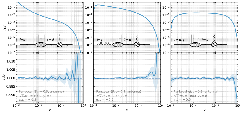
Figure 1: Ratio of the DGLAP evolution produced by the parton shower versus the DGLAP evolution as calculated with HOPPET. The results are shown as a function of the momentum fraction $x$ carried by the parton extracted from the proton. The forward evolution in our HOPPET-based reference calculation is constrained to end with the ${\hat{\imath}}=\bar{d}$ flavour, such that it reflects the starting point of the (backwards-evolving) shower, which we take to be $d\bar{d}$ in this case. We work with $y_{Z}=0$ and $\sqrt{s}/m_{Z}=1000$, such that the maximal $x$ fraction a parton can have is $0.001$. We take $\lambda=\alpha_{s}L=-0.5$. The three columns then show different extracted flavours $i$ that led to this ${\hat{\imath}}=\bar{d}$ state, where we focus on the $i=\bar{d}$ (left), $i=g$ (middle) and $i\neq\{\bar{d},g\}$ (right) cases. We show the PanGlobal shower with ${\beta_{\text{{ps}}}}=0$ (upper panels), and the PanLocal dipole shower with ${\beta_{\text{{ps}}}}=0.5$ (lower panels).

For the purpose of comparing the shower to the DGLAP expectation we are free to use either Eq. (12) or the direct shower-record information on the incoming parton $x$ after showering. We choose the latter because it also gives easy access to the flavour information. We show results with a tiny value of $\alpha_{s}=5\times 10^{-6}$ and a large value of $L=-10^{5}$, so as to render negligible any terms beyond single-logarithmic accuracy.

We obtain the DGLAP prediction using the HOPPET evolution code Salam:2008qg , which provides a straightforward way to evaluate Eq. (11), as long as one ensures that $x$ is not too close to ${\hat{x}}$, to avoid systematic effects associated with HOPPET’s discretisation. The HOPPET evolution is performed at single logarithmic accuracy, i.e. leading-order (LO) evolution in the standard DGLAP nomenclature. Since LO DGLAP evolution is purely single logarithmic, we are free to use any finite $\alpha_{s}$ such that $\alpha_{s}L=-0.5$ as in the shower. The treatment of PDFs, both in the shower and within HOPPET, is further discussed in Appendix A. In particular, our approach for handling PDFs when working at very small $\alpha_{s}$ values and large logarithms is discussed in Appendix A.2, while the choice of PDFs at the evolution starting scale is described in Appendix A.3.

Results are shown in Fig. 1. We take $\sqrt{s}/m_{Z}=1000$ and $y_{Z}=0$ such that ${\hat{x}}=0.001$, and set ${\hat{\imath}}=\bar{d}$. We then consider three scenarios: the flavour of the incoming parton remained the same ($i=\bar{d}$); it became a gluon ($i=g$), which implies that at least one flavour-changing splitting occurred; or it became any other flavour ($i\neq\bar{d},g$), which implies that at least two flavour-changing splittings occurred. The results are shown for the PanGlobal ${\beta_{\text{{ps}}}}=0$ and the PanLocal (dipole) ${\beta_{\text{{ps}}}}=0.5$ showers (similar results are obtained for the other showers, including both IF-recoil options of Dipole-$k_{t}$). We obtain agreement with the predictions of standard DGLAP evolution (with LO evolution, i.e. NLL accuracy in our context) to within statistical accuracy. The size of the statistical error depends on the value of the PDFs, and is below $0.1\%$ in a substantial part of the $x$ range, but increases in regions where the PDF is small or the flavour in question is accessible only in rare events.

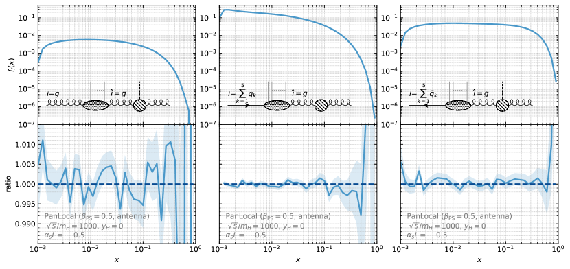
Figure 2: Same as Fig. 1 but with the $gg\rightarrow H$ process.

For completeness Fig. 2 shows the distributions for $gg\rightarrow H$ events with $\sqrt{s}/m_{H}=1000$ and $y_{H}=0$, where we examine $i=g$, the sum over quarks $i=\sum_{k}q_{k}$, and the sum over anti-quarks $i=\sum_{k}\bar{q}_{k}$. Again, the agreement is good to within statistical errors, both for the PanScales showers (shown) and the standard Dipole-$k_{t}$ showers (not shown). We have also tested different values of $\lambda$ and $\sqrt{s}$.

4 NLL tests for global observables

A range of important collider observables belong to the class of “global observables”, so-called because they are sensitive to radiation in the whole of phase space. These observables vanish in the absence of any radiation. They include phenomenologically important quantities such as the colour-singlet transverse momentum and the leading-jet transverse momentum. It is therefore of critical importance to understand the logarithmic accuracy of showers for these observables.

Global observables share the feature that the probability (or cumulative distribution) for a (dimensionless) observable $O$ to take a value smaller than ${\rm e}^{L}$ can be written as Catani:1992ua ; Banfi:2004yd

$$\Sigma(O<e^{L})\equiv\Sigma(\alpha_{s},\alpha_{s}L)=H(\alpha_{s})\exp\left[-Lg_{1}(\alpha_{s}L)+g_{2}(\alpha_{s}L)+\mathcal{O}(\alpha_{s}^{n}L^{n-1})\right]+\dots,$$ (13)

where the ellipses denote corrections that are suppressed by powers of $e^{L}$ (recall that $L$ is large and negative). The function $H(\alpha_{s})$ is the hard function multiplying the resummed series and we shorten $\alpha_{s}(m_{X}^{2})\equiv\alpha_{s}$. One may take $H(\alpha_{s})=1$ at NLL accuracy. In general, the N^kLL function $\alpha_{s}^{k-1}g_{k+1}(\alpha_{s}L)$ resums terms of $\alpha_{s}^{n}L^{n-k+1}$. In order to validate the NLL accuracy of the shower, we examine the ratio of the parton shower evaluation of $\Sigma$ to the analytic NLL evaluation, and check whether that ratio converges to 1 when one extrapolates $\alpha_{s}\to 0$.

In this section we concentrate on observables measured on the hadronic final state. Given its particular phenomenological importance and subtle analytic resummation properties, the discussion of the transverse momentum of the $Z/H$ boson is deferred to Section 5. All of the tests here use $\sqrt{s}=5m_{X}$ and $y_{X}=0$. We have also carried out a number of tests with $y_{X}=2$, which give identical results, so we do not display them here.

4.1 Leading jet transverse momentum and the azimuthal difference between the two leading jets

We start by considering the transverse momentum, $p_{t1}$, of the hardest jet in the colour-singlet production the process. The quantity $\Sigma(p_{t1})$ corresponds to the efficiency of a jet veto in colour-singlet production processes — recall that jet vetoes are widely used to reduce backgrounds to Higgs and other electroweak production processes (e.g. backgrounds with leptons and missing energy from top-quark production, which inevitably also involve jets). Here we consider jets defined with the Cambridge/Aachen (C/A) algorithm with $R=1$ Dokshitzer:1997in ; Wobisch:1998wt , keeping in mind that the NLL prediction is independent of the jet radius $R$ and is the same Banfi:2012yh for all members of the generalised-$k_{t}$ family, including the anti-$k_{t}$ algorithm Cacciari:2008gp . In Fig. 3(a) we show the $\alpha_{s}\to 0$ extrapolation for the ratio of the shower cumulative distribution to the NLL result, for the $pp\to Z$ process. We see that the PanScales showers reproduce the analytic answer, i.e. $\lim_{\alpha_{s}\to 0}\Sigma_{\text{PS}}/\Sigma_{\text{NLL}}=1$. That is not the case for Dipole-$k_{t}$ showers, with discrepancies of up to $20\%$ for global IF recoil at extreme values of $\lambda$, and $25\%$ with the local IF recoil Dipole-$k_{t}$ variant.

One comment is that these significant effects are in a region corresponding to jet transverse momenta of the order of a few GeV, which is much smaller than typical jet veto scales. However, jet activity at such low momenta is relevant also in studies of multiple interactions and the underlying event CMS:2017ngy ; ATLAS:2019ocl . Specifically, underlying event studies often examine energy and charged-particle flow in different azimuthal regions of the event, defined with respect to the $Z$ transverse direction. Another context in which azimuthal correlations are important is in the identification of ridge-like structures in high-multiplicity $pp$ collisions CMS:2010ifv ; ATLAS:2015hzw .

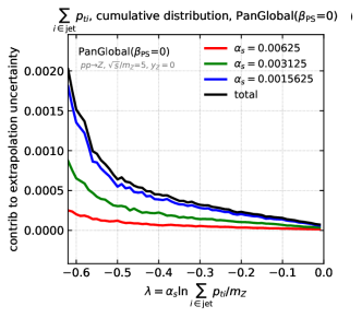
(a)

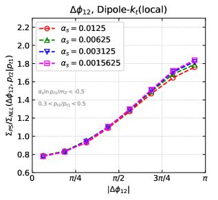
(b)

Figure 3: (a) Ratio of the shower and NLL results for the cumulative distribution for the hardest jet transverse momentum, $p_{t1}$, with $-0.62<\lambda<0$ and $\alpha_{s}\to 0$ for $pp\to Z$ events. (b) Difference in azimuthal angles between the two leading jets in a $pp\to Z$ event, where the first jet has $\lambda=\alpha_{s}\ln p_{t1}/m_{Z}\leq-0.5$, while the second one has $0.3\leq\frac{p_{t2}}{p_{t1}}\leq 0.5$. In the $\alpha_{s}\to 0$ limit, the $\lambda<-0.5$ condition effectively fixes $\lambda=-0.5$. In both plots, we have shifted the horizontal locations of the markers for the two PanLocal showers, so as to avoid having all the symbols overlap.

To give some insight into possible azimuthal structures induced by parton showers, we study a specific observable, namely the distribution of the difference in azimuthal angles between the two highest-$p_{t}$ jets, $\Delta\phi_{12}$. At NLL, this distribution is flat in $|\Delta\phi_{12}|$ and reads

$$\Sigma(\Delta\phi_{12},p_{t2}|p_{t1})\equiv\frac{\Sigma(\Delta\phi_{12},p_{t2},p_{t1})}{\Sigma(p_{t1})}=\frac{1}{\pi}\left(e^{2C_{i}R_{0}^{\prime}(-b_{0}\lambda)\ln p_{t2}^{\max}/p_{t1}}-e^{2C_{i}R_{0}^{\prime}(-b_{0}\lambda)\ln p_{t2}^{\min}/p_{t1}}\right),$$ (14)

with the $R_{0}^{\prime}$ function as given in Eq. (37a). Fig. 3(b) shows the $\alpha_{s}\to 0$ limit of that distribution, normalised to the NLL result, for events where $\alpha_{s}\ln p_{t1}/m_{Z}<-0.5$ and $0.3<p_{t2}/p_{t1}<0.5$. Again we see that the PanScales showers reproduce the NLL expectation. The Dipole-$k_{t}$ showers do not, with up to 85% (55%) discrepancies when a local (global) IF recoil is employed, a consequence of the way in which they perform the transverse momentum recoil. Note that in the $\alpha_{s}\to 0$ limit, the two jets that are relevant for Fig. 3(b) are nearly always both soft and well separated in rapidity. Consequently, at NLL accuracy, the observable is not affected by spin correlations.

A final comment in this section is that the NLL discrepancies that we observe for the IF-global Dipole-$k_{t}$ variant are expected (and observed) to be the same as those for related observables in $e^{+}e^{-}$ collisions Dasgupta:2020fwr (modulo the fact that the latter’s results were at leading colour, while here we use the NODS colour scheme Hamilton:2020rcu ). Indeed, the choice of the evolution variable, as well as the dipole being partitioned in its rest frame, is common to both initial- and final-state formulations, at least in the soft-and-collinear limit relevant for these NLL discrepancies.

4.2 Generic global event shapes

Next, we discuss a wider range of global event shape observables. For this purpose, it is useful to introduce three families of observables:

$$S_{p,\beta_{\text{obs}}} =\!\!\!\!\sum_{i\in\text{partons}}\frac{p_{ti}}{Q}{\rm e}^{-\beta_{\rm obs}|y_{i}-y_{X}|}\,,$$ (15a)

$$S_{j,\beta_{\text{obs}}} =\sum_{i\in\text{jets}}\frac{p_{ti}}{Q}{\rm e}^{-\beta_{\rm obs}|y_{i}-y_{X}|}\,,$$ (15b)

$$M_{j,\beta_{\text{obs}}} =\max_{i\in\text{jets}}\frac{p_{ti}}{Q}{\rm e}^{-\beta_{\rm obs}|y_{i}-y_{X}|}\,,$$ (15c)

where $p_{ti}$ and $y_{i}$ are respectively the transverse momentum and rapidity of parton or jet $i$, $y_{X}$ is the rapidity of the colour-singlet system, and jets are again defined with the C/A algorithm with $R=1$. The “$S$” observables involve a sum over either particles or jets, while the “$M$” observables examine a maximum across jets. Each family is parametrised by a variable $\beta_{\text{obs}}$, which determines the relative weighting of central versus forward particles/jets. Note that $M_{j,0}$ coincides with the transverse momentum of the hardest jet shown in Fig. 3(a), while $S_{p,1}$ coincides with the widely studied $0$-jettiness ($\tau_{0}$) of Ref. Stewart:2010tn , which is also used in the Geneva Alioli:2012fc ; Alioli:2013hqa matching procedure. For all of the observables, the LL resummation structure depends on $\beta_{\text{obs}}$. For a given value of $\beta_{\text{obs}}$, the $M_{j,\beta_{\text{obs}}}$ observables differ from the $S_{p,\beta_{\text{obs}}}$ and $S_{j,\beta_{\text{obs}}}$ at NLL, while the $S_{p,\beta_{\text{obs}}}$ and $S_{j,\beta_{\text{obs}}}$ observables differ from NNLL onwards. The resummation formulas up to NLL are summarised in Appendix B.

In our numerical tests, we take $\beta_{\text{obs}}=0,0.5,1$. In Fig. 4 we show the ratio of the shower to the NLL result for the cumulative distribution $\Sigma(O<e^{L})$, as calculated in the limit $\alpha_{s}\to 0$ for $\lambda=-0.5$. As in the final-state case Dasgupta:2020fwr , we find that standard dipole showers fail to reproduce the all-order NLL results for $\beta_{\text{obs}}=0$ observables, as represented by the red squares. This failure is a consequence of incorrect assignment of transverse recoil to earlier emissions vanBeekveld:2022zhl . Its impact on logarithmic terms can be examined analytically with a fixed-order study analogous to that in the final-state case Dasgupta:2018nvj . Concerning the $\beta_{\text{obs}}=0.5,1$ cases, the $\alpha_{s}\to 0$ dipole-shower results appear to agree with the NLL predictions. However the studies of similar observables in the final-state case showed that dipole-type showers induce spurious all-order leading-colour super-leading logarithms, $(\alpha_{s}L)^{n}(\alpha_{s}L^{2})^{p}$ (Section 2-d of the supplementary material of Ref. Dasgupta:2020fwr ). Because these issues arise from the soft-collinear region, which is effectively treated identically in the final-state and (global-IF) initial-state cases, they will inevitably arise also in the initial-state case (for local-IF recoil, we expect similar problems). Accordingly we colour these dipole-shower points in amber. The green circles for the four PanScales showers in Fig. 4 indicate that their predictions are in agreement with the NLL results, and the analysis of recoil in Ref. vanBeekveld:2022zhl ensures the absence of the fixed-order issues that cause us to colour the dipole showers in amber.

As a final remark, we remind the reader that in these studies, subleading $N_{c}$ corrections have been included according to the NODS method Hamilton:2020rcu for both the dipole-type showers and the PanScales showers, so as to concentrate on the impact of recoil. In contrast, standard dipole showers choose the colour factor according to whether the emitting dipole end that is closer (in the dipole centre-of-mass frame) is a gluon ($C_{A}/2$) or a quark ($C_{F}$). This results in incorrect terms already at LL, in analogy with the final-state discussion in Ref. Dasgupta:2018nvj . The numerical impact will be the same as in the all-order final-state study Hamilton:2020rcu .

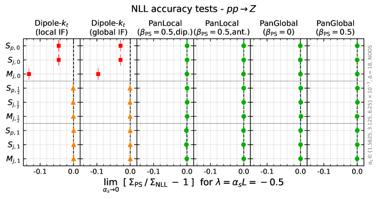
Figure 4: Summary of deviations from NLL for several global observables for the process $q\bar{q}\to Z$ and $\lambda=-0.5$. Red squares denote a clear NLL failure; amber triangles indicate a NLL fixed-order failure that is masked at all orders; green circles are used when the shower passed both the numerical NLL tests and the fixed-order recoil tests. The $\alpha_{s}\to 0$ result is obtained by quadratically extrapolating the shower results at $\alpha_{s}=0.00625,0.003125$ and $0.0015625$, and includes a systematic error that is evaluated as the change in the $\alpha_{s}\to 0$ extrapolation when one uses $\alpha_{s}=0.0125$ instead of $\alpha_{s}=0.003125$. The showers include a dynamic cutoff $\Delta=18$, which functions as discussed in our earlier $e^{+}e^{-}$ tests Dasgupta:2020fwr ; Hamilton:2020rcu .

5 The transverse momentum of the colour-singlet system

The next observable that we discuss is the cumulative distribution for the transverse momentum of a massive colour singlet (here, $Z$ or $H$ boson) produced in proton collisions. It has wide relevance for LHC phenomenology, and for example its understanding is critical for $W$ mass extractions ATLAS:2017rzl ; LHCb:2021bjt ; CDF:2022hxs . It is also widely used in matching showers and fixed-order calculations Hamilton:2012rf ; Monni:2019whf ; Buonocore:2022mle ; Alioli:2021qbf .

The colour singlet $p_{tX}$ distribution is a more subtle observable than those studied in the previous subsections, essentially because it has two resummation regimes. In one of the regimes, that with moderately small $p_{tX}$, the suppression of the cross section is driven dominantly by the Sudakov suppression of emissions and the NLL prediction can be written in terms of our standard resummation formula, Eq. (13), where $L=\ln p_{tX}/m_{X}$. The other regime concerns asymptotically small values of $p_{tX}$, which are typically obtained by a vector cancellation between the recoils from two or more gluons emitted with $p_{t}$’s substantially larger than $p_{tX}$. In this regime, Eq. (13) breaks down Frixione:1998dw , and the NLL resummation instead generally requires $b$-space resummation Parisi:133268 , giving a result for $\Sigma$ that scales as $p_{tX}^{2}$. The transition between the two regimes occurs where $R^{\prime}=|\partial_{L}(Lg_{1}(\alpha_{s}L))|=2$ and it is reflected in a $1/(R^{\prime}-2)$ divergence in the $g_{2}(\alpha_{s}L)$ function of Eq. (13), cf. Eqs. (31) and (39) of Appendix B. The location of the transition corresponds to $\lambda\simeq-0.48$ for $Z$ production and $\lambda\simeq-0.32$ for Higgs production (both for $n_{f}=5$). In the region of moderately small $p_{tX}$ (“Sudakov region”) we will carry out our tests in the same way as earlier, while for asymptotically small $p_{tX}$ (“power-scaling region”) we will adopt a somewhat different procedure. We start with the former.

5.1 Sudakov region

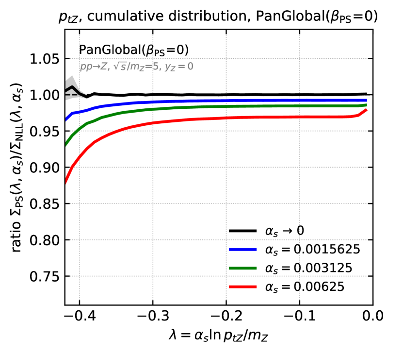
(a)

(b)

Figure 5: Ratio of the cumulative distribution for the colour-singlet transverse momentum to the NLL analytic result, in the $\alpha_{s}\to 0$ limit, for (a) $q\bar{q}\to Z$ and (b) $gg\to H$ events. The results are shown for Dipole-$k_{t}$ with local (red dashed line) and global recoil (green dotted line), PanGlobal with $\beta_{\text{PS}}=0$ (blue solid line) and $\beta_{\text{PS}}=0.5$ (blue circles), and PanLocal with $\beta_{\text{PS}}=0.5$, both for the antenna (black triangles) and dipole (black squares) variants. For clarity, the PanLocal antenna (dipole) points have been slightly shifted towards the left (right), with respect to the values actually used, which coincide with the PanGlobal ${\beta_{\text{{ps}}}}=0.5$ ones.

In Fig. 5 we show the $\alpha_{s}\to 0$ extrapolation of the ratio of the shower to the NLL prediction for the colour singlet transverse momentum, with a range of showers. The results are shown for $q\bar{q}\to Z$ (Fig. 5(a)) and $gg\to H$ (Fig. 5(b)). We use Eq. (13) as our NLL reference together with ingredients from Eqs. (29a), (31) (using $\beta_{\text{obs}}=0$), and Eq. (39). We consider only $\lambda\geq-0.42$ ($Z$) and $\lambda\geq-0.26$ ($H$), to stay well away from the breakdown of the $p_{tX}$-space NLL resummation. The PanScales showers that are shown all agree with the NLL prediction. Conversely, the Dipole-$k_{t}$ showers fail to reproduce the correct NLL result. For the $q\bar{q}\to Z$ process, we see a 35% (10%) discrepancy of the NLL terms at $\lambda=-0.42$ using the Dipole-$k_{t}$ shower with a local (global) recoil. For the $gg\to H$ process we find a 7% (3%) difference at $\lambda=-0.26$. Performing a comparison at the same value of $\lambda=-0.25$ for both processes, we find a $3\%$ ($1\%$) discrepancy for $q\bar{q}\to Z$ versus $7\%$ ($2\%$) for $gg\to H$, with local (global) IF recoil in the Dipole-$k_{t}$ shower.

5.2 Power-scaling region

Now let us turn to the second resummation regime, namely that where $R^{\prime}>2$ and the dominant mechanism to produce a small $p_{tX}$ is a vector cancellation between the transverse recoils of different emissions. A first remark is that the tests shown in Fig. 5 already probe this mechanism, because the NLL result is sensitive to it even in the regime of $R^{\prime}<2$, through the $g_{2}$ function in Eq. (13), specifically the part in Eq. (39). Still, the $R^{\prime}>2$ regime is conceptually important and it is therefore of interest to explicitly examine the behaviours of different showers.

It is useful to recall the structure of the standard $b$-space result for the resummation of the transverse-momentum distribution Parisi:133268 ; Collins:1984kg ; Bozzi:2005wk ,

$$\frac{{\rm d}\Sigma}{{\rm d}p_{tX}^{2}}=\int_{0}^{\infty}\frac{{\rm d}b}{2}bJ_{0}(bp_{tX})\Sigma_{V}(b_{0}/b)\,,$$ (16)

with $b_{0}=2{\rm e}^{-\gamma_{E}}$, $\Sigma_{V}$ the $b$-space resummed distribution, and $J_{0}$ the Bessel function of the first kind and order $0$. Observe that for $p_{tX}\to 0$ the result tends to a non-zero constant, whose value can be straightforwardly obtained by replacing $J_{0}(bp_{tX})\to 1$ in Eq. (16). Fig. 6(a) shows the small-$p_{tX}$ behaviour of the distribution for $Z$ production, in four showers. Three of them, PanGlobal, PanLocal and Dipole-$k_{t}$(global), indeed tend to a non-zero constant. In contrast the variant of Dipole-$k_{t}$ with local recoil for IF dipoles tends to zero in this limit, i.e. it has the wrong scaling behaviour. This is because, after the first emission, the event consists of two IF dipoles, and from that point onwards, no further transverse recoil is taken by the $Z$ boson. Therefore the only mechanism for $p_{tZ}$ to be small is Sudakov suppression of the first emission, which is a much stronger suppression than the vector cancellation.

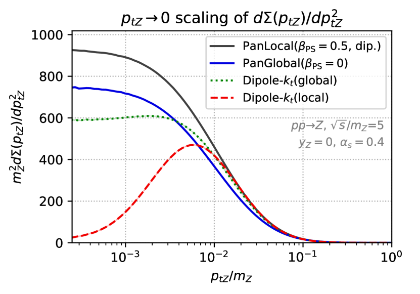
(a)

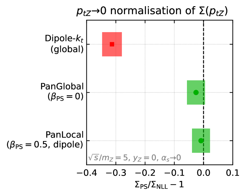
(b)

Figure 6: (a) $m_{Z}^{2}d\Sigma(p_{tZ})/d{p_{tZ}^{2}}$, as determined with four showers. In QCD this quantity tends to a calculable (non-zero) constant for $p_{tZ}\to 0$ Parisi:133268 . (b) For the three showers that tend to a non-zero constant, the plot shows the $\alpha_{s}\to 0$ limit of the deviation of that constant relative to the NLL expectation, with the usual (red) green colour coding for (dis)agreement with NLL.

For those showers that do tend to a non-zero constant, it is worth checking the value of that constant, which is a prediction of the NLL resummation. The expected value can be deduced from Eq. (16), simply setting $p_{tX}=0$ on the right-hand side. Note that at our NLL accuracy, $\Sigma_{V}$ coincides with the cumulative distribution of the leading jet $p_{t}$, or equivalently (still at NLL), in a $p_{t}$-ordered shower, the shower ordering variable. We use the distribution of the latter (or a transverse-momentum like analogue in ${\beta_{\text{{ps}}}}=0.5$ showers) to evaluate Eq. (16), because it facilitates the $\alpha_{s}\to 0$ extrapolation.

To determine the asymptotic normalisation of the shower, one needs to evaluate the height of the plateau in Fig. 6(a). As can be seen in the plot, this is somewhat delicate because on one hand the approach to the asymptotic value is fairly slow, and on the other hand the statistical errors grow rapidly at small $p_{tZ}$. For each value of $\alpha_{s}$ that we study, we estimate the ratio of the shower plateau height to the NLL expectation in a $p_{tZ}$ region where Eq. (16) is within $3\%$ of its asymptotic value, assigning as a systematic error the change induced when increasing $\ln p_{tZ}$ by one. We then perform a linear extrapolation of the $\alpha_{s}=0.2$ and $0.3$ ratios to obtain the ratio at $\alpha_{s}=0$, with a further systematic obtained from the change in the result when instead using $\alpha_{s}=0.2$ and $0.4$. Finally, we account for the fact that the plateau is determined in a region that is $3\%$ away from the asymptotic region with a further overall $3\%$ systematic error (which ultimately dominates the total error). The final ratios, with total statistical and systematic errors are shown in Fig. 6(b). The PanGlobal (${\beta_{\text{{ps}}}}=0$) and PanLocal (${\beta_{\text{{ps}}}}=0.5$) showers are consistent with the NLL expectation, while the Dipole-$k_{t}$ shower (with global IF recoil) clearly has the wrong normalisation.

The reader will have noticed that in contrast with all other results in this paper, the results here have been obtained with quite large values of the coupling. Furthermore the coupling has been kept fixed in the shower (and in the associated PDF translation). This is because it is considerably more difficult to simultaneously explore $\alpha_{s}\to 0$ and $p_{tX}\to 0$ than for other observables. Furthermore, at large values of $\alpha_{s}$, had we used a running coupling, we would have had to disentangle logarithmic effects from power-suppressed but potentially non-negligible effects associated with the regularisation of $\alpha_{s}$ near the Landau pole.

6 Single non-global logarithms for a rapidity-slice

Many standard hadron collider observables are non-global, i.e. sensitive to radiation in restricted parts of angular phase space. For example, almost any isolation criterion for leptons or photons involves restricting the energy flow in a region around the object. Measurements of the top mass, as obtained from decay kinematics, inevitably use jets that miss some radiation from the decay products. For all of these observables, the resummation involves non-global logarithms Dasgupta:2001sh ; Dasgupta:2002bw , which can only be correctly reproduced with dipole showers Banfi:2006gy .

To assess the ability of the shower to capture non-global logarithms (NGLs), we compute the scalar sum of the transverse momenta $p_{ti}$ of the final-state particles in a rapidity slice (excluding the colour-singlet particle) Dasgupta:2002bw ; Dasgupta:2001sh . Taking $\Delta$ to be the half-width of a slice centred at the rapidity, $y_{X}$, of the colour-singlet system, we define the observable as

$$S^{\rm slice}_{\Delta}=\sum_{i\in\text{partons}}p_{ti}\,\Theta(\Delta-|y_{i}-y_{X}|)\,.$$ (17)

The NGLs are single-logarithmic terms of the form $\lambda^{n}=\alpha_{s}^{n}L^{n}$, where $L=\ln(p_{t}/Q)$, created by the emissions of soft large-angle gluons near the edge of the slice and we obtain our reference resummation from the code developed for Ref. Caletti:2021oor , which uses the strategy of Ref. Dasgupta:2001sh .

To test the shower accuracy, we take a rapidity-slice window of full-width 2 ($\Delta=1$) and scan over values of $-0.5<\lambda=\alpha_{s}L<0$. Fig. 7(a) shows PanGlobal ${\beta_{\text{{ps}}}}=0$ shower results, as compared to the single logarithmic expectations, illustrating perfect agreement across the full range of $\lambda$. Fig. 7(b) shows results for several showers at a fixed value of $\lambda=-0.5$, demonstrating that all showers agree with the expected result. The Dipole-$k_{t}$ showers are coloured amber because they fail to pass fixed-order tests (see Ref. Dasgupta:2020fwr ) and are subject to spurious leading-colour super-leading logarithms.

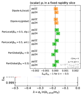
(a)

(b)

Figure 7: (a) Cumulative distribution for the transverse-momentum in a rapidity slice of $|y-y_{X}|<1$ as a function of $\lambda$ for the PanGlobal ${\beta_{\text{{ps}}}}=0$ shower. The top panel shows the expected (dashed) and the shower (solid) results, and the bottom panel shows the ratio between the two. (b) Difference between the shower $\Sigma_{\rm PS}$ and the expected single-logarithmic result ($\Sigma_{\rm SL}$) for a fixed value of $\lambda=-0.5$ for all showers. Colour coding is the same as in Fig. 4.

Note that this is the only one of our tests that has been performed at leading colour ($C_{F}=C_{A}/2=4/3$) rather than full colour. The NODS scheme used elsewhere in this article is fully accurate for non-global logarithms in colour singlet production only up to and including $\alpha_{s}^{2}$. Nevertheless, in $e^{+}e^{-}$ collisions it was found to be numerically very close Hamilton:2020rcu to the full-colour result Hatta:2013iba for non-global observables. For a corresponding full-colour comparison in hadron collisions, one would need an extension of the results of Ref. Hatta:2020wre to include Coulomb/Glauber-gluon related (coherence-violating) $i\pi$ terms, or of Refs. Becher:2021zkk or Nagy:2019bsj to processes without hard Born jets.

7 Particle (or subjet) multiplicity

The particle multiplicity is one of the most fundamental observables at any collider. At hadron colliders specifically, a good understanding of the particle multiplicity from the hard process is important in accurately extracting the properties of the underlying event. From a theoretical point of view, with a well-defined infrared cutoff, the resummation structure of particle multiplicity is very similar to that of subjet multiplicity, and our tests here effectively apply to both.

From an analytic perspective, the resummation structure of multiplicity differs from all other observables presented above since its cumulative distribution cannot be written in the form of Eq. (13), and its logarithmic accuracy has to be determined at the level of $\Sigma$ rather than $\ln\Sigma$. The analogue of Eq. (13) for such non-exponentiating observables is

$$\Sigma(L)=h_{1}(\alpha_{s}L^{2})+\sqrt{\alpha_{s}}h_{2}(\alpha_{s}L^{2})+\dots,$$ (18)

where the N^kDL function $\alpha_{s}^{k/2}h_{k+1}(\alpha_{s}L^{2})$ resums terms of $\alpha_{s}^{n}L^{2n-k}$. That is, the function $h_{1}$ captures the double logarithmic (DL) enhancement, $h_{2}$ the next-to-double-logarithmic (NDL) contribution and so on. In the multiplicity case, the logarithm that needs to be resummed is $L=\ln(k_{t,{\text{cut}}}/m_{X})$, where, up to NDL accuracy, $k_{t,{\text{cut}}}$ may be either a shower transverse momentum cutoff (for particle multiplicities) or a jet algorithm transverse momentum cut for a suitably defined subjet multiplicity.

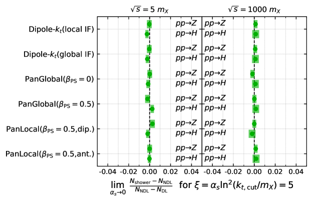
Figure 8: Extrapolation of $\frac{N_{\text{shower}}-N_{{\rm NDL}}}{N_{\rm NDL}-N_{\rm DL}}$ to $\alpha_{s}=0$ at a fixed value of $\xi=\alpha_{s}L^{2}$ for all showers, two different energies ($\sqrt{s}=5m_{X}$, left, and $\sqrt{s}=1000m_{X}$, right), and the two processes under study, i.e. $pp\to Z$ and $pp\to H$.

Recently, the subjet multiplicity in colour singlet production has been computed up to NDL accuracy Medves:2022ccw (earlier calculations gave similar structures Catani:1991pm ; Catani:1993yx ; Forshaw:1999iv ). In a shower context, up to NDL, it applies equally well to the number of particles in the event ($N_{\text{shower}}$) when one sets the strong coupling to zero below a given value of $k_{t,\text{cut}}$.

To test the NDL terms in Eq. (18), we compute the following ratio

$$\frac{N_{\text{shower}}-N_{{\rm NDL}}}{N_{\rm NDL}-N_{\rm DL}},$$ (19)

which vanishes in the $\alpha_{s}\to 0$ limit if the shower is correct at NDL accuracy. The result of computing Eq. (19) with all showers, at two different energies and for two different hard processes ($pp\to Z$ and $pp\to H$) is shown in Fig. 8. We observe that all showers are consistent with the full-colour NDL expectation, within the small statistical errors. Relative to our other tests, the critical feature of the multiplicity is that it probes the soft-collinear nested structure of the shower. At NDL accuracy, it also probes the hard-collinear correction to the splitting function, the 1-loop running of the coupling, the DGLAP evolution of PDFs, and the colour scheme. Since these features are common across all of our showers, no discrepancy is expected between the PanScales showers and Dipole-$k_{t}$, and none is observed.

8 Exploratory phenomenological results with toy PDFs

A proper phenomenological study of the PanScales showers would require a number of elements that are not yet mature, such as the inclusion of quark-mass effects and interfacing to a program such as Pythia Sjostrand:2014zea ; Bierlich:2022pfr so as to include hadronisation and multi-parton interactions. Nevertheless, even without these effects it is still of potential interest to examine the results from the showers in a physically relevant regime rather than the regimes of extreme small coupling and large logarithms used in the body of the paper.

As parton showers become more accurate, one critical element to include in physical studies is an estimate of residual uncertainties. In the results that follow, we will include renormalisation- and factorisation-scale variation uncertainties, so as to provide one measure of residual higher-order uncertainties. However, it is important to bear in mind that these scale variations cannot account for uncertainties associated with the showers’ improper handling of the effective matrix element in various phase-space regions (e.g. the hard region, or the double-soft region). A study of how to do so robustly goes beyond the scope of this section, so instead we will use the range of variation within showers of a given logarithmic-accuracy class as an indication of such further residual uncertainties.

Our treatment of renormalisation scale variation is inspired by Mrenna:2016sih , though it differs in the details. Specifically for showers that have been established to be NLL accurate, for an emission carrying away a momentum fraction $z$, the emission strength is taken proportional to

$$\alpha_{s}(\mu_{\text{{r}}}^{2})\left(1+\frac{K\alpha_{s}(\mu_{\text{{r}}}^{2})}{2\pi}+2\alpha_{s}(\mu_{\text{{r}}}^{2})b_{0}(1-z)\ln x_{\text{{r}}}\right)\,,\qquad\mu_{\text{{r}}}=x_{\text{{r}}}\mu_{\text{{r}}}^{\text{central}},$$ (20)

where $b_{0}$ and $K$ are defined below in Appendix B, Eqs. (30). This factor generalises the factor $\alpha_{s}(\mu_{\text{{r}}}^{2})(1+K\alpha_{s}(\mu_{\text{{r}}}^{2})/(2\pi))$ in Eq. (2.3) of vanBeekveld:2022zhl , which was given for the central choice $\mu_{\text{{r}}}\equiv\mu_{\text{{r}}}^{\text{central}}=\rho v{\rm e}^{{\beta_{\text{{ps}}}}|\bar{\eta}_{Q}|}$ (i.e. $x_{\text{{r}}}=1$ in Eq. (20)), cf. Eq. (B.27) of vanBeekveld:2022zhl . The reason for including a factor $(1-z)$ in the compensation term of Eq. (20) (i.e. the term proportional to $b_{0}$), is that it ensures that scale compensation is active for soft emissions, $z\to 0$, but not for hard emissions, where one would need the higher-order ingredients such as those from Ref. Dasgupta:2021hbh in order to justify the inclusion of scale-compensating terms. For LL showers we will include the $K$ term, but not the scale compensation term proportional to $b_{0}$. The justification for this is that a soft emission’s $k_{t}$ is not preserved after subsequent emissions and therefore one cannot unambiguously identify the correct scale-dependent terms for a given emission. All showers use 2-loop evolution of the coupling. We take $\alpha_{s}(m_{Z})=0.118$ and we implement an infrared cutoff on the shower by setting $\alpha_{s}(\mu_{\text{{r}}})=0$ for $\mu_{\text{{r}}}<x_{\text{{r}}}\times 0.5\;\mathrm{GeV}$.

We will use a 5-flavour PDF and a 5-flavour running of the coupling, so as to avoid complications related to the handling of flavour thresholds. The PDF used for the results in this section has the initial condition of Eq. (26) at a scale of $\mu_{\text{{f}}}=0.5\;\mathrm{GeV}$, evolved to higher scales with HOPPET. Aside from the issue of having $5$ flavours down to the infrared cutoff, it is reasonably similar to a physical PDF, however not to the extent that one can make direct comparisons with data. Accordingly the results here should be interpreted in terms of their broad trends, rather than specific values at any given phase space point. Factorisation scale variations are implemented by adding an $\ln x_{\text{{f}}}$ term to the expression for $\ln\mu_{\text{{f}}}$ in Eq. (B.1) of vanBeekveld:2022zhl , as used in Eq. (2.3) of that paper. The scale variations that we use in the plots are a 5-point set, $(x_{\text{{r}}},x_{\text{{f}}})=\{(1,1),(1/2,1),(2,1),(1,1/2),(1,2)\}$ and we will use the envelope generated by this set as our overall scale uncertainty band.

In the logarithmic accuracy tests in this paper, we have used the NODS colour scheme for all showers, including the Dipole-$k_{t}$ showers. Here, we retain that choice for PanScales showers, but instead use the colour-factor from emitter scheme in the Dipole-$k_{t}$ case, as this is the colour scheme adopted by standard dipole showers.

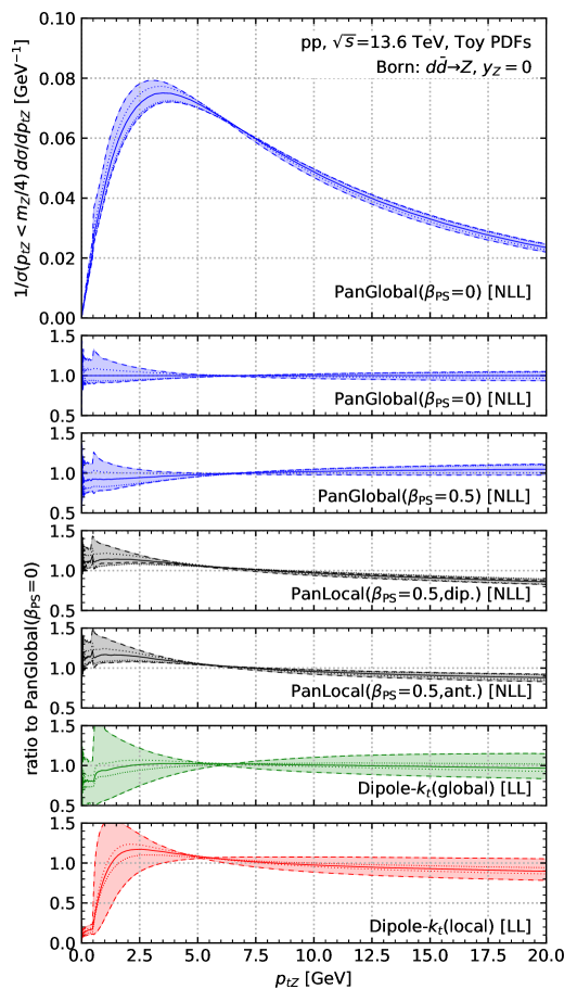
Figure 9: The $p_{tZ}$ distribution as predicted in a variety of parton showers. The plots use a semi-physical setup, for a $pp$ centre-of-mass energy $13.6\;\mathrm{TeV}$. The Born events involve $d\bar{d}$ scattering with a $Z$ rapidity of zero, and the showers use 5-flavour toy PDFs defined through the initial condition of Eq. (26) at a scale of 0.5 GeV. The top panel shows the $p_{tZ}$ distribution with the PanGlobal (${\beta_{\text{{ps}}}}=0$) shower and the remaining panels show the ratio to that distribution for each of several showers. For each shower, the band corresponds to the envelope of the renormalisation scale ($x_{\text{{r}}}$) variations (dashed lines) and factorisation scale ($x_{\text{{f}}}$) variations (dotted lines), as described in the text.

We will consider two observables: the interjet $\Delta\phi_{12}$ distribution of Section 4.1 and the transverse momentum of the $Z$-boson, $p_{tZ}$, as discussed in Section 5. Let us start with the $p_{tZ}$ distribution, given its broad phenomenological importance. The top panel of Fig. 9 shows the $p_{tZ}$ distribution for the PanGlobal (${\beta_{\text{{ps}}}}=0$) shower, normalised to the integral of the distribution up to $p_{tZ}=m_{Z}/4$. The reason for this normalisation is to reduce sensitivity of the results to the high $p_{t}$ region, where fixed-order matching would be required to obtain a reliable prediction. Each of the remaining panels shows the ratio of a given parton shower (with is scale variations) to the $x_{\text{{r}}}=x_{\text{{f}}}=1$ PanGlobal (${\beta_{\text{{ps}}}}=0$) result.

The first feature of Fig. 9 that we comment on is that the scale uncertainty bands are significantly smaller for the NLL PanScales parton showers than for the LL dipole-$k_{t}$ showers. This is because only the NLL showers include the $b_{0}$ scale-compensation term in the renormalisation scale uncertainty of Eq. (20). Next, we observe variations from one NLL shower to the next, by an amount commensurate with the renormalisation and factorisation scale uncertainties. This is a consequence of different approximations for shower elements that are beyond NLL (for example the effective treatment of the double soft region, the specific mapping from shower scale to transverse momentum in the hard collinear region, and the absence of matching to the hard $Z+\text{jet}$ matrix elements). The final comment concerns the LL showers: for the Dipole-$k_{t}$ (global) shower, the central value (solid curve) is rather similar to that from the PanGlobal showers. This is consistent with the observations in Figs. 5(a) and 6(a), from which one expected $\sim 10\%$ agreement of Dipole-$k_{t}$(global) with the PanGlobal shower, except in the deepest part of the infrared region. In contrast, the Dipole-$k_{t}$ (local) shower shows larger differences, also as expected, notably in the different scaling behaviour at low $p_{t}$ values, $p_{tZ}\lesssim 2\;\mathrm{GeV}$. One should keep in mind that for phenomenological applications, some of this difference might be absorbed into a tune of intrinsic transverse momentum of partons within the proton. However doing so might well be physically wrong, since the intrinsic transverse momentum manifests itself in the final state through counterbalancing transverse momentum assigned to the proton remnant (i.e. concentrated just at high rapidity) rather than to soft gluon radiation (i.e. spread across all rapidities).

In practical high-precision applications, parton showers results are often reweighted so as to reproduce high-accuracy resummation and fixed-order predictions for $p_{tZ}$ Bizon:2019zgf ; Alioli:2021qbf ; Re:2021con ; Becher:2020ugp ; Camarda:2021ict ; Billis:2021ecs ; Ebert:2020dfc ; Chen:2018pzu ; Chen:2022cgv ; Ju:2021lah ; Neumann:2022lft . However, for a given $p_{tZ}$, such reweighting leaves the pattern of final-state emissions unchanged. Therefore it is also of interest to study the structure of the final state. We do so in Fig. 10, looking at the difference in azimuth between the two leading jets, $\Delta\phi_{12}$. This is a close analogue of the distribution studied in Section 4.1, but adapted so as to be phenomenologically realistic. Specifically, we cluster all final-state partons (excluding the $Z$-boson) with the anti-$k_{t}$ algorithm Cacciari:2008gp with a radius of $R=0.4$, as implemented in FastJet 3.4 Cacciari:2011ma . We consider only jets with $|y|<2.5$, require at least two jets, where the hardest has $20<p_{t1}<30\;\mathrm{GeV}$ and the second hardest has $0.3<p_{t2}/p_{t1}<0.5$. We also require a minimum rapidity separation between the jets, $|\Delta y_{12}|>1$, so as to reduce the impact of large-angle $g\to gg$ (and $q\bar{q}$) splitting and to eliminate jet-clustering induced artefacts associated with a suppression of the distribution for $\Delta\phi_{12}<R$. We then consider the distribution of $\Delta\phi_{12}$, normalised to the number of events that passed the cuts. This is shown in Fig. 10(a) for an on-shell $Z$. Fig. 10(b) shows similar results, but with two changes: a stronger requirement on the separation between the two leading jets, $|\Delta y_{12}|>1.5$, to further reduce the impact of large-angle $g\to gg/q\bar{q}$ splitting (uncontrolled because the showers lack the double-soft matrix element); and replacing on-shell $Z$-bosons with off-shell $Z$-bosons with an invariant mass of $500\;\mathrm{GeV}$, so that the $20\;\mathrm{GeV}$ jets are less affected by the lack of hard matrix element corrections.

(a)

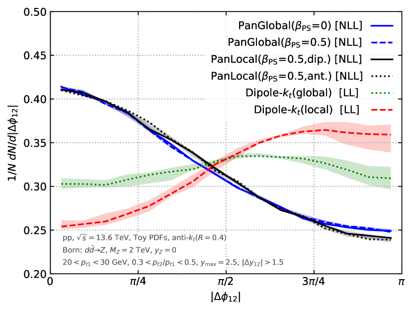
(b)

Figure 10: The $\Delta\phi_{12}$ distribution between the two leading jets, for events that pass the cuts described in the text, (a) for events on the $Z$ pole and a requirement $|\Delta y_{12}|>1.0$, and (b) for events where the $Z$ is off-shell, with an invariant mass of $500\;\mathrm{GeV}$, and a requirement $|\Delta y_{12}|>1.5$. The bands correspond to the variation of renormalisation and factorisation scales. Most of the impact of this variation vanishes because the plots are normalised to the number of events that pass the cuts and instead it is the differences between showers within a given logarithmic accuracy class that better provides a measure of residual shower uncertainties.

The two plots in Fig. 10 can be compared to their analogue in the asymptotic logarithmic limit, Fig. 3(b). One caveat is that the former normalises to the cross section for the jets to pass the transverse momentum and rapidity selection cuts (as would most likely be done experimentally), while the latter normalises to the asymptotic NLL expectation of Eq. (14), which is simple only in the absence of rapidity cuts on the jets. A first feature to comment on is that in Fig. 10, the PanScales showers are not flat in $\Delta\phi_{12}$, unlike the case in Fig. 3(b). This is because in a non-negligible fraction of the events with two jets passing the cuts, those two jets effectively came from a large-angle $g\to gg$ (or $q\bar{q}$) splitting, and so have $\Delta\phi_{12}$ close to $0$, resulting in the enhancement seen in that region. We have verified that increasing the $\Delta y_{12}$ cut, e.g. to $2$, leads to a degree of flattening of the distribution for all of the PanScales showers, as does eliminating the $|y|<2.5$ selection on the jets (which increases the relative contribution of configurations with large rapidity separations). Among the PanScales showers there is some spread between the showers in Fig. 10(a), notably between the PanGlobal variants on one hand and the PanLocal variants on the other. This spread largely vanishes when probing a more asymptotic kinematic region, Fig. 10(b), and further investigation shows that the reduction of spread stems both from the increase in colour singlet mass and the $\Delta y_{12}$ requirement. Note that the renormalisation and factorisation scale variation are far from encompassing the spread in Fig. 10(a) (in part because the scale variations are divided out by the normalisation). This is a sign that scale variation alone is not sufficient for probing the uncertainties in parton showers, as in many other contexts, and that one also needs to investigate uncertainties related to uncontrolled limits of matrix elements.

To close our discussion, we turn to the Dipole-$k_{t}$ results in Fig. 10. The variant with local-IF recoil has a substantially different shape from the NLL showers. Even though the shape differs from the asymptotic limit in Fig. 3(b) (again because of residual $g\to gg/q\bar{q}$ splittings), the enhancement at $\Delta\phi_{12}\simeq\pi$, relative to the NLL showers, is qualitatively as expected from that plot. In contrast, we see that the Dipole-$k_{t}$ variant with global-IF recoil in Fig. 10(a) is fairly similar to the NLL showers. In this kinematic region, the logarithms are not yet very large. As a result the smaller LL versus NLL differences (for this observable) of the Dipole-$k_{t}$(global) shower as compared to Dipole-$k_{t}$(local), are commensurate with the beyond-NLL differences between PanScales showers. However, the results in Fig. 10(a), if taken alone, would give a false sense of confidence in the phenomenological adequacy of the Dipole-$k_{t}$(global) shower for this observable. In particular exploring a more asymptotic kinematic region, as in Fig. 10(b), reveals clear differences also between Dipole-$k_{t}$(global) and the NLL PanScales showers.

9 Conclusions

In this article, we have carried out over a dozen distinct all-order tests of the logarithmic accuracy of parton showers for colour-singlet production at hadron colliders.

On one hand, these tests were designed to probe distinct classes of next-to-leading logarithmic effects, covering all of the main aspects that a shower should be able to handle. On the other, each of the observables also connects with important phenomenological aspects of LHC physics. The tests probed nested emissions in the hard collinear region (DGLAP tests of Section 3); nested emissions in the soft large-angle region (non-global observables of Section 6); nested emissions in both the soft and collinear regions (multiplicities of Section 7); and the higher-order structure of double logarithmic Sudakov resummation, including both recoil and the scale and scheme of the coupling in the Sudakov form factor (global observables of Sections 4 and 5). All of these tests were carried out with the NODS colour scheme of Ref. Hamilton:2020rcu , and with comparisons to full-colour resummation (with the exception of non-global observables).

For the PanLocal shower (with ${\beta_{\text{{ps}}}}=0.5$) and the PanGlobal showers (${\beta_{\text{{ps}}}}=0$ and $0.5$), all tests were successful. For the Dipole-$k_{t}$ showers, we considered two variants, one with dipole-local (“local”), the other with event-wide (“global”) recoil in initial–final dipoles. Both had visible discrepancies relative to NLL for all global observables that connect directly with transverse momentum measurements. This includes the jet veto acceptance (Fig. 3(a)), a number of generic global observables (Fig. 4) and the colour-singlet transverse momentum distribution (Figs. 5 and 6). Note that our Dipole-$k_{t}$ tests used our NODS colour scheme. Had we used the colour treatment that is effectively standard for dipole showers (colour-factor-from-emitter in the language of Ref. Hamilton:2020rcu ), we would also have seen subleading-$N_{\text{{c}}}$ issues in the Dipole-$k_{t}$ showers at LL for $\beta_{\text{obs}}>0$ global observables, NLL for $\beta_{\text{obs}}=0$ and DL for multiplicities.

A number of steps remain for practical phenomenological applications of the PanScales showers. These include the matching to fixed-order calculations, the extension of our validations and tests to hadron-collider processes with final-state jets, the inclusion of finite quark masses and the interface to hadronisation and multi-particle-interaction models. Nevertheless, the advances presented here provide an important step in the formulation and validation of NLL-accurate showers for hadron collisions. The first exploration of the phenomenological impact of our NLL showers in Section 8 shows some of the potential benefits from the control of logarithmic accuracy.

Appendix A Parton distribution functions

The inclusion of a ratio of parton distribution functions in the branching kernel for initial-state emissions is a vital component of a complete hadronic parton shower. While the PanScales showers follow the backwards evolution in much the same way that all other widely-used showers do, the numerical demands on the implementation are often of a very different order. Below, we discuss some of the numerical details in our handling of PDFs. Appendix A.1 outlines our procedure for overestimating the PDF ratio that appears in the branching kernels. Appendix A.2 outlines how we obtain PDFs for use in limits with extreme values of the logarithm and tiny values of $\alpha_{s}$. Finally, Appendix A.3 provides the specific functional form that we use for our PDFs when testing logarithmic accuracy.

A.1 Overestimating the PDF ratio

In the PanScales formalism, the differential branching probability for initial-state emissions may be written as

$${\rm d}\mathcal{P}_{{\tilde{\imath}}{\tilde{\jmath}}\to ijk}=\frac{\alpha_{s}(k_{\perp}^{2})}{2\pi}\left(1+\frac{\alpha_{s}(k_{\perp}^{2})K}{2\pi}\right)\frac{{\rm d}v^{2}}{v^{2}}{\rm d}\eta\frac{{\rm d}\varphi}{2\pi}\times\\ \times\frac{x_{i}f_{i}(x_{i},\mu^{2})}{\tilde{x}_{i}f_{{\tilde{\imath}}}(\tilde{x}_{i},\mu^{2})}\frac{x_{j}f_{j}(x_{j},\mu^{2})}{\tilde{x}_{j}f_{{\tilde{\jmath}}}(\tilde{x}_{j},\mu^{2})}\left[g(\eta)z_{i}P^{\rm{IS/FS}}_{ik}(z_{i})+g(-\eta)z_{j}P^{\rm{IS/FS}}_{jk}(z_{j})\right]\,,$$ (21)

where $\mu$ is the factorisation scale to be used in the PDFs and the rest of the notation is as in Ref. vanBeekveld:2022zhl . To implement these branchings in the shower using the standard veto algorithm, an overestimate is required for the branching probability. In the absence of the PDF ratios (i.e. for final-state branchings), the branching probability is easily overestimated by a constant, $\alpha_{s}C_{A}/\pi$. This is not quite as straightforward anymore when the PDF ratio is included. The shower is maximally efficient if the overestimate is as tight as possible, but it will not produce the correct distributions if regions exist where the branching probability is not correctly overestimated.

We implement a solution that maintains the simplicity of the final-state case as much as possible by introducing a further overhead factor $C^{\text{PDF}}(\tilde{x},{\tilde{\imath}})$ that depends on the current longitudinal momentum fraction $\tilde{x}$ of an initial-state parton, as well as its flavour ${\tilde{\imath}}$. The generic overestimate constant $\alpha_{s}C_{A}/\pi$ is multiplied by this overhead factor, and the acceptance probability is divided by it.

The overhead factor is evaluated by filling grids with values of $C^{\text{PDF}}(\tilde{x},{\tilde{\imath}})$ for all ${\tilde{\imath}}$s and for equally-spaced values of $-\ln 2\tilde{x}$ for $\tilde{x}<1/2$, or $-\ln 2(1-\tilde{x})$ for $\tilde{x}>1/2$. Then, for every pair $(\tilde{x},{\tilde{\imath}})$ in the grid, a secondary grid scan is performed over $x>\tilde{x}$ and all factorisation scales that can be accessed in the shower, so as to identify the maximum branching weight given in Eq. (21). Once a maximum is found, another grid search is performed in the cell of the previously-identified maximum. This process is repeated four times and the result is then multiplied by a margin factor $1.2$ and stored in the $C^{\text{PDF}}(\tilde{x},{\tilde{\imath}})$ grid.

At the beginning of the shower evolution and after every shower branching, an adequate overhead factor can then be determined by probing the $C^{\text{PDF}}(\tilde{x},{\tilde{\imath}})$-grid at the current longitudinal momentum fraction and flavour of the initial-state partons. While this procedure is not guaranteed to determine an overestimate over all of phase space, we find that the modest margin factor of $1.2$ avoids any issues without significant detriment to efficiency. This method is applicable in principle to any reasonably well-behaved PDF set, as long as we remain in a region of fixed number of flavours, i.e. stay away from potential mass threshold effects that can cause the overhead factor to diverge. For our all-order tests, we make use of the toy PDFs given in Appendix A.3.

A.2 PDFs at extreme scales

Standard PDF evolution tools are not well-suited to our requirements of being able to evaluate PDF ratios in the limit where $\alpha_{s}\to 0$ with $\alpha_{s}L$ fixed. At the accuracy we intend to probe, NLL or NDL, it is sufficient to make use of PDFs with purely collinear, single-logarithmic DGLAP evolution. This means that only leading-order splitting functions and 1-loop running of $\alpha_{s}$ are required. In this situation, the PDF evolution is a function purely of an evolution time parameter $t=\alpha_{s}L$. We can leverage this fact to evaluate PDFs at extremely small scales without having to explicitly perform the DGLAP evolution to those scales.

In what follows we use $\mu$ to denote a factorisation scale within the shower (which operates over asymptotic scales) and $\mu_{\text{{pdf}}}$ to denote a factorisation scale in the PDF evolution (which operates over standard physical scales). We start by generating a five-flavour, one-loop PDF set between a lower scale $\mu_{\text{{pdf}},0}$ and a high scale $\mu_{\text{{pdf}},1}$, with a value of $\alpha_{s,\text{{pdf}}}(\mu_{\text{{pdf}}}^{2})$ similar to the physical value. This task can be handled by DGLAP evolution codes. We choose to use the HOPPET library Salam:2008qg . The PDF scale $\mu_{\text{{pdf}},1}$ is then mapped onto the shower initial hard transverse momentum scale $\mu_{1}$. Lower scales are then related by

$$t_{\text{{pdf}}}(\mu_{\text{{pdf}}}|\mu_{\text{{pdf}},1})=t_{\text{shower}}(\mu|\mu_{1})\,.$$ (22)

At the NLL accuracy that we are aiming for, where it is sufficient to use one-loop DGLAP evolution, the left-hand side is given by

$$t_{\text{{pdf}}}(\mu_{\text{{pdf}}}|\mu_{\text{{pdf}},1})=\int^{\mu_{\text{{pdf}},1}}_{\mu_{\text{{pdf}}}}\frac{{\rm d}q}{q}\frac{\alpha_{s,\text{{pdf}}}(q^{2})}{\pi}=\frac{-\ln\left(1+\beta_{0}\,\alpha_{s,\text{{pdf}}}(\mu_{\text{{pdf}},1}^{2})\ln\mu_{\text{{pdf}}}^{2}/\mu_{\text{{pdf}},1}^{2}\right)}{2\pi\beta_{0}}\,,$$ (23)

and we have

$$\mu_{\text{{pdf}}}(\mu)=\mu_{\text{{pdf}},1}\exp\left(\frac{\alpha_{s}(\mu_{1}^{2})}{\alpha_{s,\text{{pdf}}}(\mu_{\text{{pdf}},1}^{2})}\ln\frac{\mu}{\mu_{1}}\right),$$ (24)

where $\alpha_{s}(\mu_{1}^{2})$ is the value of the coupling used in the shower evolution at the hard scale $(\mu_{1})$. The shower PDF can then be evaluated as

$$f_{i}(x,\mu^{2}_{\text{{pdf}}}(\mu))\,.$$ (25)

The choice of the numerical values of $\mu_{\text{{pdf}},1}$, $\mu_{\text{{pdf}},0}$ and $\alpha_{s,\text{{pdf}}}(\mu_{\text{{pdf}},1}^{2})$ is somewhat arbitrary, only requiring that the DGLAP evolution is performed over a range that is wide enough to cover the kinematic range of the shower, and that the evolution is numerically stable. The above procedure then facilitates consistent comparison of shower runs with a variety of values of $\alpha_{s}(\mu_{1}^{2})$, as long as the upper boundary of the shower, $\mu_{1}$, always remains anchored to the same PDF scale $\mu_{\text{{pdf}},1}$.

A.3 PDF choice

We employ a toy PDF set whose functional form is defined at the starting scale for the evolution $\mu_{\text{{pdf}},0}=1\;\mathrm{GeV}$, with the coupling at that scale set to $\alpha_{s}(\mu_{\text{{pdf}},0}^{2})=0.5$. For the gluon PDF at that scale we take

$$g(x) =N_{g}\,x^{\beta}\,(1-x)^{5}\,,$$ (26a)

with $$\beta=-0.1 N_{g}=1.7$$ and . For the quark PDFs we define

$$u_{v}(x) =N_{u_{v}}\,x^{\alpha}\,(1-x)^{3}\,,$$ (26b)

$$d_{v}(x) =N_{d_{v}}\,x^{\alpha}\,(1-x)^{4}\,,$$ (26c)

$$\tilde{d}(x) =N_{\bar{d}}\,x^{\beta}\,(1-x)^{6}\,,$$ (26d)

$$\tilde{u}(x) =N_{\bar{d}}\,x^{\beta}\,(1-x)^{7}\,,$$ (26e)

with $$\alpha=0.8 N_{u_{v}}=5.1072 N_{d_{v}}=3.06432 N_{\bar{d}}=0.1939875$$, , and . We then use

$$u(x) =u_{v}(x)+0.8\tilde{u}(x)\,,$$ (26f)

$$d(x) =d_{v}(x)+0.8\tilde{d}(x)\,,$$ (26g)

$$\bar{u}(x) =0.8\tilde{u}(x)\,,$$ (26h)

$$\bar{d}(x) =0.8\tilde{d}(x)\,,$$ (26i)

$$s(x) =\bar{s}(x)=0.2(d(x)+\tilde{d}(x))\,,$$ (26j)

$$c(x) =\bar{c}(x)=b(x)=\bar{b}(x)=0.15(\tilde{u}(x)+\tilde{d}(x))\,,$$ (26k)

$$t(x) =\bar{t}(x)=0\,.$$ (26l)

In the above equations the forms for the PDFs are all implicitly to be understood as being at the factorisation scale $\mu_{\text{{pdf}},0}$. The PDF uses $n_{f}=5$ light flavours, as with the rest of our results in this paper. For the purposes of mapping shower scales to PDF scales, as in Appendix A.2, we use $\mu_{\text{{pdf}},1}=10^{7}\;\mathrm{GeV}$.

Appendix B Resummation formulae

In this appendix we summarise the NLL analytic resummation expressions used in Section 4. We consider a continuously global observable Banfi:2004yd that, for a single soft or collinear emission with transverse momentum $k_{t}$ and rapidity $y$ takes the form

$$O=\frac{k_{t}}{Q}e^{-\beta_{\text{obs}}|y-y_{X}|},$$ (27)

with $0\leq\beta_{\text{obs}}\leq 1$ and $y_{X}$ the rapidity of the massive colour-singlet boson. The probability that the observable is smaller than $e^{L}$, where $L$ is taken to be large and negative, can be written at NLL accuracy as

$$\Sigma(\alpha_{s},\alpha_{s}L)=\exp\left[-Lg_{1}(\alpha_{s}L)+g_{2}(\alpha_{s}L)+\mathcal{O}(\alpha_{s}^{n}L^{n-1})\right]$$ (28)

The $g_{1}$-function contains the LL terms and reads

$$g^{\beta_{\text{obs}}=0}_{1} =2C_{i}\left[\frac{1}{2\pi b_{0}\bar{\lambda}}\left(2\bar{\lambda}+\ln(1-2\bar{\lambda})\right)\right]\,,$$ (29a)

$$g^{\beta_{\text{obs}}\neq 0}_{1} =2C_{i}\left[\frac{1}{2\pi b_{0}\bar{\lambda}\beta_{\text{obs}}}\left((1+\beta_{\text{obs}}-2\bar{\lambda})\ln\left(1-\frac{2\bar{\lambda}}{1+\beta_{\text{obs}}}\right)-(1-2\bar{\lambda})\ln(1-2\bar{\lambda})\right)\right]\,,$$ (29b)

with

$$b_{0}=\frac{11C_{A}-4n_{f}T_{R}}{12\pi}\,,\quad\quad\bar{\lambda}=-b_{0}\alpha_{s}L=-b_{0}\lambda\,,$$ (30)

and $C_{i}=C_{A}(C_{F})$ for Higgs ($Z$) production.

The NLL corrections in Eq. (28) are resummed in the $g_{2}$-function. This function contains contributions from (i) soft-collinear emissions $r_{2}$, (ii) hard-collinear emissions $T$, (iii) the PDF evolution $\mathcal{L}$, and (iv) a factor $\mathcal{F}_{\beta_{\rm obs}}$ that accounts for the way the observable depends on multiple emissions. It takes the general form

$$g_{2}=-2C_{i}r_{2}(\bar{\lambda})-2C_{i}B_{i}T\left(\bar{\lambda}\right)+\ln\mathcal{L}+\ln\mathcal{F}_{\beta_{\text{obs}}}\,,$$ (31)

with $C_{i}$ the same as above, $B_{i}=B_{q}=-3/4$ for quarks and $B_{g}=(-11C_{A}+4n_{f}T_{R})/12C_{A}$ for gluons. The NLL contribution from soft-collinear emissions reads

$$r_{2}^{\beta_{\text{obs}}=0} =\frac{1}{2\pi b_{0}^{2}}\left[\frac{K}{2\pi}\left(\ln(1-2\bar{\lambda})+\frac{2\bar{\lambda}}{1-2\bar{\lambda}}\right)-\frac{b_{1}}{b_{0}}\left(\frac{1}{2}\ln^{2}(1-2\bar{\lambda})+\frac{\ln(1-2\bar{\lambda})+2\bar{\lambda}}{1-2\bar{\lambda}}\right)\right]\,,$$ (32a)

$$r_{2}^{\beta_{\text{obs}}\neq 0} =\frac{1}{2\pi b_{0}^{2}\beta_{\text{obs}}}\Bigg{[}\frac{K}{2\pi}\left((1+\beta_{\text{obs}})\ln\left(1-\frac{2\bar{\lambda}}{1+\beta_{\text{obs}}}\right)-\ln(1-2\bar{\lambda})\right)$$

$$+\frac{b_{1}}{b_{0}}\Bigg{(}\frac{1}{2}\ln^{2}(1-2\bar{\lambda})-\frac{1}{2}(1+\beta_{\text{obs}})\ln^{2}\left(1-\frac{2\bar{\lambda}}{1+\beta_{\text{obs}}}\right)+\ln(1-2\bar{\lambda})$$

$$-(1+\beta_{\text{obs}})\ln\left(1-\frac{2\bar{\lambda}}{1+\beta_{\text{obs}}}\right)\Bigg{)}\Bigg{]},$$ (32b)

with

$$b_{1}=\frac{17C_{A}^{2}-10C_{A}n_{f}T_{R}-6C_{F}n_{f}T_{R}}{24\pi^{2}}\,,\qquad K=\left(\frac{67}{18}-\frac{\pi^{2}}{6}\right)C_{A}-\frac{10}{9}n_{f}T_{R}\,,$$ (33)

while the corresponding term for hard-collinear emissions is given by

$$T=-\frac{1}{\pi b_{0}}\ln\left(1-\frac{2\bar{\lambda}}{1+\beta_{\rm obs}}\right)\,.$$ (34)

The contribution arising from the PDFs evolution in processes with two coloured legs in the initial state ($\ell_{1,2}$) is given by

$$\ln\mathcal{L}=\ln\left(\frac{f_{\ell_{1}}\!\left(x_{1},Q^{2}e^{2L/(1+\beta_{\text{obs}})}\right)}{f_{\ell_{1}}(x_{1},Q^{2})}\right)+\ln\left(\frac{f_{\ell_{2}}\!\left(x_{2},Q^{2}e^{2L/(1+\beta_{\text{obs}})}\right)}{f_{\ell_{2}}(x_{2},Q^{2})}\right),$$ (35)

and $f_{\ell_{i}}(x_{i},\mu^{2})$ the PDF for flavour $\ell_{i}$ evaluated for a light cone momentum fraction $x_{i}$ at the factorisation scale $\mu$. In conjunction with our PDF mapping from Appendix A.2, Eq. (35) depends on the logarithm of the observable only through the value of $\lambda$. The last term of Eq. (31) depends on the type of observable. For an additive observable we have

$$\ln\mathcal{F}_{\beta_{\text{obs}}}^{S}=-\gamma_{E}R^{\prime}(\bar{\lambda})-\ln\Gamma\left(1+R^{\prime}(\bar{\lambda})\right)\,,$$ (36)

with $R^{\prime}(\bar{\lambda})$ defined as $\partial_{L}\left(-Lg_{1}(\bar{\lambda})\right)$, i.e.

$$R^{\prime}_{\beta_{\text{obs}}=0}(\bar{\lambda}) =\frac{4C_{i}}{\pi b_{0}}\frac{\bar{\lambda}}{1-2\bar{\lambda}}\,,$$ (37a)

$$R^{\prime}_{\beta_{\text{obs}}\neq 0}(\bar{\lambda}) =\frac{2C_{i}}{\pi b_{0}\beta_{\text{obs}}}\left[\ln\left(1-\frac{2\bar{\lambda}}{1+\beta_{\text{obs}}}\right)-\ln(1-2\bar{\lambda})\right].$$ (37b)

For observables involving a maximum among jets, i.e. the $M_{j,\beta_{\text{obs}}}$ of Eq. (15c), we have

$$\ln\mathcal{F}_{\beta_{\text{obs}}}^{M}=0\,.$$ (38)

The transverse momentum of the colour singlet also belongs to the class of global observables with $\beta_{\text{obs}}=0$. In this case, the observable-dependent correction reads

$$\ln\mathcal{F}_{\beta_{\text{obs}}}^{p_{tX}}=-\gamma_{E}R^{\prime}(\bar{\lambda})-\ln\Gamma\left(1+R^{\prime}(\bar{\lambda})/2\right)+\ln\Gamma\left(1-R^{\prime}(\bar{\lambda})/2\right)\,,$$ (39)

which has pole at $R^{\prime}(\bar{\lambda})=2$.

References

- (1) M. van Beekveld, S. Ferrario Ravasio, G. P. Salam, A. Soto-Ontoso, G. Soyez and R. Verheyen, PanScales parton showers for hadron collisions: formulation and fixed-order studies, 2205.02237.
- (2) T. Sjostrand, S. Mrenna and P. Z. Skands, PYTHIA 6.4 Physics and Manual, JHEP 05 (2006) 026, [hep-ph/0603175].
- (3) W. T. Giele, D. A. Kosower and P. Z. Skands, A simple shower and matching algorithm, Phys. Rev. D78 (2008) 014026, [0707.3652].
- (4) S. Schumann and F. Krauss, A Parton shower algorithm based on Catani-Seymour dipole factorisation, JHEP 03 (2008) 038, [0709.1027].
- (5) S. Platzer and S. Gieseke, Coherent Parton Showers with Local Recoils, JHEP 01 (2011) 024, [0909.5593].
- (6) S. Hoeche and S. Prestel, The midpoint between dipole and parton showers, Eur. Phys. J. C75 (2015) 461, [1506.05057].
- (7) B. Cabouat and T. Sjöstrand, Some Dipole Shower Studies, Eur. Phys. J. C78 (2018) 226, [1710.00391].
- (8) K. Hamilton, R. Medves, G. P. Salam, L. Scyboz and G. Soyez, Colour and logarithmic accuracy in final-state parton showers, JHEP 03 (2021) 041, [2011.10054].
- (9) Z. Nagy and D. E. Soper, On the transverse momentum in Z-boson production in a virtuality ordered parton shower, JHEP 03 (2010) 097, [0912.4534].
- (10) M. Dasgupta, F. A. Dreyer, K. Hamilton, P. F. Monni and G. P. Salam, Logarithmic accuracy of parton showers: a fixed-order study, JHEP 09 (2018) 033, [1805.09327].
- (11) M. Dasgupta, F. A. Dreyer, K. Hamilton, P. F. Monni, G. P. Salam and G. Soyez, Parton showers beyond leading logarithmic accuracy, Phys. Rev. Lett. 125 (2020) 052002, [2002.11114].
- (12) A. Karlberg, G. P. Salam, L. Scyboz and R. Verheyen, Spin correlations in final-state parton showers and jet observables, Eur. Phys. J. C 81 (2021) 681, [2103.16526].
- (13) K. Hamilton, A. Karlberg, G. P. Salam, L. Scyboz and R. Verheyen, Soft spin correlations in final-state parton showers, JHEP 03 (2022) 193, [2111.01161].
- (14) I. W. Stewart, F. J. Tackmann and W. J. Waalewijn, N-Jettiness: An Inclusive Event Shape to Veto Jets, Phys. Rev. Lett. 105 (2010) 092002, [1004.2489].
- (15) G. Parisi and R. Petronzio, Small transverse momentum distributions in hard processes, Nucl. Phys. B 154 (Feb, 1979) 427–440. 21 p.
- (16) G. Gustafson and U. Pettersson, Dipole Formulation of QCD Cascades, Nucl. Phys. B306 (1988) 746–758.
- (17) S. Catani and M. H. Seymour, A General algorithm for calculating jet cross-sections in NLO QCD, Nucl. Phys. B485 (1997) 291–419, [hep-ph/9605323].
- (18) S. Catani, S. Dittmaier, M. H. Seymour and Z. Trocsanyi, The Dipole formalism for next-to-leading order QCD calculations with massive partons, Nucl. Phys. B 627 (2002) 189–265, [hep-ph/0201036].
- (19) J. C. Collins, Spin Correlations in Monte Carlo Event Generators, Nucl. Phys. B304 (1988) 794–804.
- (20) I. Knowles, Angular Correlations in QCD, Nucl. Phys. B 304 (1988) 767–793.
- (21) I. Knowles, Spin Correlations in Parton - Parton Scattering, Nucl. Phys. B 310 (1988) 571–588.
- (22) I. G. Knowles, A Linear Algorithm for Calculating Spin Correlations in Hadronic Collisions, Comput. Phys. Commun. 58 (1990) 271–284.
- (23) G. P. Salam and J. Rojo, A Higher Order Perturbative Parton Evolution Toolkit (HOPPET), Comput. Phys. Commun. 180 (2009) 120–156, [0804.3755].
- (24) Yu. L. Dokshitzer and G. Marchesini, Monte Carlo and large angle gluon radiation, JHEP 03 (2009) 117, [0809.1749].
- (25) P. Z. Skands and S. Weinzierl, Some remarks on dipole showers and the DGLAP equation, Phys. Rev. D79 (2009) 074021, [0903.2150].
- (26) S. Catani, L. Trentadue, G. Turnock and B. R. Webber, Resummation of large logarithms in e+ e- event shape distributions, Nucl. Phys. B407 (1993) 3–42.
- (27) A. Banfi, G. P. Salam and G. Zanderighi, Principles of general final-state resummation and automated implementation, JHEP 03 (2005) 073, [hep-ph/0407286].
- (28) Y. L. Dokshitzer, G. D. Leder, S. Moretti and B. R. Webber, Better jet clustering algorithms, JHEP 08 (1997) 001, [hep-ph/9707323].
- (29) M. Wobisch and T. Wengler, Hadronization corrections to jet cross-sections in deep inelastic scattering, in Workshop on Monte Carlo Generators for HERA Physics (Plenary Starting Meeting), pp. 270–279, 4, 1998. hep-ph/9907280.
- (30) A. Banfi, G. P. Salam and G. Zanderighi, NLL+NNLO predictions for jet-veto efficiencies in Higgs-boson and Drell-Yan production, JHEP 06 (2012) 159, [1203.5773].
- (31) M. Cacciari, G. P. Salam and G. Soyez, The anti- jet clustering algorithm, JHEP 04 (2008) 063, [0802.1189].
- (32) CMS collaboration, A. M. Sirunyan et al., Search for supersymmetry in final states with two oppositely charged same-flavor leptons and missing transverse momentum in proton-proton collisions at 13 TeV, JHEP 04 (2021) 123, [2012.08600].
- (33) ATLAS collaboration, G. Aad et al., Search for chargino–neutralino pair production in final states with three leptons and missing transverse momentum in TeV pp collisions with the ATLAS detector, Eur. Phys. J. C 81 (2021) 1118, [2106.01676].
- (34) CMS collaboration, A. M. Sirunyan et al., Measurement of the underlying event activity in inclusive Z boson production in proton-proton collisions at TeV, JHEP 07 (2018) 032, [1711.04299].
- (35) ATLAS collaboration, G. Aad et al., Measurement of distributions sensitive to the underlying event in inclusive -boson production in pp collisions at TeV with the ATLAS detector, Eur. Phys. J. C 79 (2019) 666, [1905.09752].
- (36) CMS collaboration, V. Khachatryan et al., Observation of Long-Range Near-Side Angular Correlations in Proton-Proton Collisions at the LHC, JHEP 09 (2010) 091, [1009.4122].
- (37) ATLAS collaboration, G. Aad et al., Observation of Long-Range Elliptic Azimuthal Anisotropies in 13 and 2.76 TeV Collisions with the ATLAS Detector, Phys. Rev. Lett. 116 (2016) 172301, [1509.04776].
- (38) S. Alioli, C. W. Bauer, C. J. Berggren, A. Hornig, F. J. Tackmann, C. K. Vermilion et al., Combining Higher-Order Resummation with Multiple NLO Calculations and Parton Showers in GENEVA, JHEP 09 (2013) 120, [1211.7049].
- (39) S. Alioli, C. W. Bauer, C. Berggren, F. J. Tackmann, J. R. Walsh and S. Zuberi, Matching Fully Differential NNLO Calculations and Parton Showers, JHEP 06 (2014) 089, [1311.0286].
- (40) ATLAS collaboration, M. Aaboud et al., Measurement of the -boson mass in pp collisions at TeV with the ATLAS detector, Eur. Phys. J. C 78 (2018) 110, [1701.07240].
- (41) LHCb collaboration, R. Aaij et al., Measurement of the W boson mass, JHEP 01 (2022) 036, [2109.01113].
- (42) CDF collaboration, T. Aaltonen et al., High-precision measurement of the W boson mass with the CDF II detector, Science 376 (2022) 170–176.
- (43) W. Bizon, A. Gehrmann-De Ridder, T. Gehrmann, N. Glover, A. Huss, P. F. Monni et al., The transverse momentum spectrum of weak gauge bosons at + NNLO, Eur. Phys. J. C 79 (2019) 868, [1905.05171].
- (44) S. Alioli, C. W. Bauer, A. Broggio, A. Gavardi, S. Kallweit, M. A. Lim et al., Matching NNLO predictions to parton showers using N3LL color-singlet transverse momentum resummation in geneva, Phys. Rev. D 104 (2021) 094020, [2102.08390].
- (45) E. Re, L. Rottoli and P. Torrielli, Fiducial Higgs and Drell-Yan distributions at N3LL′+NNLO with RadISH, JHEP 09 (2021) 108, [2104.07509].
- (46) T. Becher and T. Neumann, Fiducial resummation of color-singlet processes at N3LL+NNLO, JHEP 03 (2021) 199, [2009.11437].
- (47) S. Camarda, L. Cieri and G. Ferrera, Drell–Yan lepton-pair production: qT resummation at N3LL accuracy and fiducial cross sections at N3LO, Phys. Rev. D 104 (2021) L111503, [2103.04974].
- (48) G. Billis, B. Dehnadi, M. A. Ebert, J. K. L. Michel and F. J. Tackmann, Higgs pT Spectrum and Total Cross Section with Fiducial Cuts at Third Resummed and Fixed Order in QCD, Phys. Rev. Lett. 127 (2021) 072001, [2102.08039].
- (49) M. A. Ebert, J. K. L. Michel, I. W. Stewart and F. J. Tackmann, Drell-Yan resummation of fiducial power corrections at N3LL, JHEP 04 (2021) 102, [2006.11382].
- (50) X. Chen, T. Gehrmann, E. W. N. Glover, A. Huss, Y. Li, D. Neill et al., Precise QCD Description of the Higgs Boson Transverse Momentum Spectrum, Phys. Lett. B 788 (2019) 425–430, [1805.00736].
- (51) X. Chen, T. Gehrmann, E. W. N. Glover, A. Huss, P. F. Monni, E. Re et al., Third-Order Fiducial Predictions for Drell-Yan Production at the LHC, Phys. Rev. Lett. 128 (2022) 252001, [2203.01565].
- (52) W.-L. Ju and M. Schönherr, The qT and spectra in W and Z production at the LHC at N3LL’+N2LO, JHEP 10 (2021) 088, [2106.11260].
- (53) T. Neumann and J. Campbell, Fiducial Drell-Yan production at the LHC improved by transverse-momentum resummation at N4LL+N3LO, 2207.07056.
- (54) K. Hamilton, P. Nason, C. Oleari and G. Zanderighi, Merging H/W/Z + 0 and 1 jet at NLO with no merging scale: a path to parton shower + NNLO matching, JHEP 05 (2013) 082, [1212.4504].
- (55) P. F. Monni, P. Nason, E. Re, M. Wiesemann and G. Zanderighi, MiNNLO: a new method to match NNLO QCD to parton showers, JHEP 05 (2020) 143, [1908.06987].
- (56) L. Buonocore, M. Grazzini, J. Haag, L. Rottoli and C. Savoini, Effective transverse momentum in multiple jet production at hadron colliders, 2201.11519.
- (57) S. Frixione, P. Nason and G. Ridolfi, Problems in the resummation of soft gluon effects in the transverse momentum distributions of massive vector bosons in hadronic collisions, Nucl. Phys. B 542 (1999) 311–328, [hep-ph/9809367].
- (58) P. F. Monni, E. Re and P. Torrielli, Higgs Transverse-Momentum Resummation in Direct Space, Phys. Rev. Lett. 116 (2016) 242001, [1604.02191].
- (59) J. C. Collins, D. E. Soper and G. F. Sterman, Transverse Momentum Distribution in Drell-Yan Pair and W and Z Boson Production, Nucl. Phys. B 250 (1985) 199–224.
- (60) G. Bozzi, S. Catani, D. de Florian and M. Grazzini, Transverse-momentum resummation and the spectrum of the Higgs boson at the LHC, Nucl. Phys. B 737 (2006) 73–120, [hep-ph/0508068].
- (61) M. Dasgupta and G. Salam, Resummation of nonglobal QCD observables, Phys. Lett. B 512 (2001) 323–330, [hep-ph/0104277].
- (62) M. Dasgupta and G. P. Salam, Accounting for coherence in interjet flow: A Case study, JHEP 03 (2002) 017, [hep-ph/0203009].
- (63) A. Banfi, G. Corcella and M. Dasgupta, Angular ordering and parton showers for non-global QCD observables, JHEP 03 (2007) 050, [hep-ph/0612282].
- (64) S. Caletti, O. Fedkevych, S. Marzani, D. Reichelt, S. Schumann, G. Soyez et al., Jet angularities in Z+jet production at the LHC, JHEP 07 (2021) 076, [2104.06920].
- (65) Y. Hatta and T. Ueda, Resummation of non-global logarithms at finite , Nucl. Phys. B874 (2013) 808–820, [1304.6930].
- (66) Y. Hatta and T. Ueda, Non-global logarithms in hadron collisions at = 3, Nucl. Phys. B 962 (2021) 115273, [2011.04154].
- (67) T. Becher, M. Neubert and D. Y. Shao, Resummation of Super-Leading Logarithms, Phys. Rev. Lett. 127 (2021) 212002, [2107.01212].
- (68) Z. Nagy and D. E. Soper, Effect of color on rapidity gap survival, Phys. Rev. D 100 (2019) 074012, [1905.07176].
- (69) R. Medves, A. Soto-Ontoso and G. Soyez, Lund and Cambridge multiplicities for precision physics, 2205.02861.
- (70) S. Catani, Y. L. Dokshitzer, F. Fiorani and B. R. Webber, Average number of jets in annihilation, Nucl. Phys. B377 (1992) 445–460.
- (71) S. Catani, Y. L. Dokshitzer and B. R. Webber, Average number of jets in deep inelastic scattering, Phys. Lett. B 322 (1994) 263–269.
- (72) J. R. Forshaw and M. H. Seymour, Subjet rates in hadron collider jets, JHEP 09 (1999) 009, [hep-ph/9908307].
- (73) T. Sjöstrand, S. Ask, J. R. Christiansen, R. Corke, N. Desai, P. Ilten et al., An Introduction to PYTHIA 8.2, Comput. Phys. Commun. 191 (2015) 159–177, [1410.3012].
- (74) C. Bierlich et al., A comprehensive guide to the physics and usage of PYTHIA 8.3, 2203.11601.
- (75) S. Mrenna and P. Skands, Automated Parton-Shower Variations in Pythia 8, Phys. Rev. D 94 (2016) 074005, [1605.08352].
- (76) M. Dasgupta and B. K. El-Menoufi, Dissecting the collinear structure of quark splitting at NNLL, JHEP 12 (2021) 158, [2109.07496].
- (77) M. Cacciari, G. P. Salam and G. Soyez, FastJet User Manual, Eur. Phys. J. C72 (2012) 1896, [1111.6097].
- (78) J. R. Forshaw, A. Kyrieleis and M. H. Seymour, Super-leading logarithms in non-global observables in QCD, JHEP 08 (2006) 059, [hep-ph/0604094].
- (79) S. Catani, D. de Florian and G. Rodrigo, Space-like (versus time-like) collinear limits in QCD: Is factorization violated?, JHEP 07 (2012) 026, [1112.4405].