Emergent Quantum Mechanics at the Boundary of a Local Classical Lattice Model

Abstract

We formulate a conceptually new model in which quantum mechanics emerges from classical mechanics. Given a local Hamiltonian $H$ acting on $n$ qubits, we define a local classical model with an additional spatial dimension whose boundary dynamics is approximately—but to arbitrary precision—described by Schrödinger’s equation and $H$. The bulk consists of a lattice of classical bits that propagate towards the boundary through a circuit of stochastic matrices. The bits reaching the boundary are governed by a probability distribution whose deviation from the uniform distribution can be interpreted as the quantum-mechanical wavefunction. Bell nonlocality is achieved because information can move through the bulk much faster than the boundary speed of light. We analytically estimate how much the model deviates from quantum mechanics, and we validate these estimates using computer simulations.

I Introduction

General relativity and the Standard Model of particle physics are not exact descriptions of reality; rather they emerge as low-energy effective field theory descriptions of some underlying theory (e.g. string theory). A characteristic signature of emergence at low energy or long time and distance scales is that the resulting physics is typically well-described by remarkably simple equations, which are often linear (e.g. the harmonic oscillator) or only consist of lowest-order terms in an effective Lagrangian.

In principle, it is possible that quantum mechanics is also only an approximate description of reality. Indeed, Schrödinger’s equation is a simple linear differential equation, suggesting that it might arise as the leading approximation to a more complete model. The advent of quantum computing opens opportunities to probe and test quantum mechanics in an unprecedented regime. Much evidence indicates that if standard quantum theory is exactly correct, then the cost of simulating a quantum computation with a classical computer must grow exponentially with the size of the quantum computer Aaronson and Chen (2016). To the extent possible, this extraordinary hypothesis about the quantum world should be tested in the laboratory. Indeed, if quantum theory actually emerges from an underlying classical model, then this exponential scaling must eventually fail for real devices. Therefore, aside from verifying Bell nonlocality Brunner et al. (2014) and studying the behavior of macroscopic superpositions Arndt and Hornberger (2014), we should also conceive and perform experiments that characterize the computational power of nature Aharonov and Vazirani (2012); Slagle (2021); ’t Hooft (2014).

Numerous experiments Lamoreaux (1992); Fry and Walther (2000); Keshavarzi et al. (2022); Shadbolt et al. (2014); Brunner et al. (2014); Arute et al. (2019); Zhu et al. (2021); Zhong et al. (2020) and theoretical observations Pusey et al. (2012); Polchinski (1991); Gisin (1990); Bremner et al. (2011); Aaronson et al. (2013); Mielnik (1974) significantly constrain, but do not completely rule out, possible deviations from standard quantum theory. For example, measurements of the anomalous magnetic dipole moment of the electron Hanneke et al. (2008) agree with quantum predictions up to roughly ten digits of precision. However, these experiments, and most other current tests of quantum theory, probe properties of matter with relatively low computational complexity, and so might be insensitive to deviations from quantum theory that become evident only for more complex states Aaronson (2004). Quantum theory also successfully predicts properties of ground states and of low-energy dynamics for many materials and molecules, but here too the detailed agreement between theory and experiment has mostly been limited to quantum states that are not profoundly entangled Lee et al. (2022); Milsted et al. (2022), and so the successful predictions do not rule out departures from quantum predictions for states of high complexity. To probe the high-complexity regime convincingly, highly excited matter should be carefully studied. It may also be necessary to measure many observables, since classically tractable models of thermalization Deutsch (2018); Srednicki (1994) and emergent hydrodynamics White et al. (2018); Leviatan et al. (2017); Rakovszky et al. (2022) may suffice for explaining the observed data when only a few degrees of freedom are measured. In contrast to more conventional experimental tools, future quantum computers that prepare highly entangled states and perform intricate measurements will be well equipped for probing the behavior of matter in the regime far beyond the reach of efficient classical simulation Arute et al. (2019); Zhu et al. (2021); Zhong et al. (2020).

Though models in which quantum dynamics emerges from underlying classical dynamics should be testable in the high complexity regime, such tests need not be applicable to other proposed modifications of standard quantum theory. For example, in models with intrinsic wavefunction collapse Bassi et al. (2013), quantum error correction Gottesman (2009) might overcome the damaging effects of the intrinsic noise, restoring the full computational power of quantum theory. Furthermore, generic non-linear corrections to Schrödinger’s equation may well enhance rather than diminish the computational power of quantum systems Abrams and Lloyd (1998), while our goal is to explore whether nature could be computationally weaker, not stronger, than standard quantum theory predicts.

Such considerations motivate the quest for testable models in which quantum mechanics emerges from classical mechanics and for which deviations from standard quantum theory are detectable in the high-complexity regime ’t Hooft (2020, 2014); Adler (2012); Vanchurin (2019, 2020); Katsnelson and Vanchurin (2021); Nelson (2012); Wolfram (2020); Hall et al. (2014); Palmer (2020); Gallego Torromé (2014). In pursuit of this quest, we aim to construct a local classical lattice model that exhibits emergent quantum mechanics (EmQM) Walleczek and Grössing (2016). We define a local classical model to consist of a lattice, where the state at each lattice site is defined by a finite list of numbers (which does not grow with the system size), and the time evolution of each lattice site only depends on the state of nearby sites. The time evolution is allowed to be stochastic and either continuous or discrete. Cellular automata and local classical lattice Hamiltonians (and Lagrangians) are examples of local classical models.

We consider a model to exhibit EmQM if its slowly-varying and long-distance physics is well-described by Schrödinger’s equation:

$$\partial_{t}\Psi=-iH\cdot\Psi.$$ (1)

$\Psi$ is the wavefunction, which encodes the state of the system, while $H$ is the Hamiltonian, which defines the dynamics.

In a sense, the classical model is performing an approximate simulation of suitably encoded Schrödinger dynamics. We want more than just that — to the extent possible we want the classical dynamics to be a reasonable model of how nature might really behave. Typical classical simulation algorithms will not fit the bill, for example because the classical dynamics is spatially non-local or because the required number of local degrees of freedom increases exponentially with system size (e.g. tensor network methods Orús (2019); Lin et al. (2022) require an exponentially large bond dimension). Drawing inspiration from neutral network algorithms Jacot et al. (2018); López Gutiérrez and Mendl (2019); Schmitt and Heyl (2020); Lin and Pollmann (2021); Jónsson et al. (2018), we seek models without such shortcomings.

We partially succeed in the following sense. Given any local Hamiltonian and initial value wavefunction for $n$ qubits in $D$ spatial dimensions, we can define a local classical lattice model in $D+1$ spatial dimensions whose $D$-dimensional boundary dynamics can be well-approximated by Schrödinger’s equation if the extra spatial dimension has a length $S$ that is exponentially large in $n$, i.e. if $S\gg 2^{n}$.

We view this as only a partial success because if $S\gg 2^{n}$ does not hold, then the boundary dynamics instead obeys a Schrödinger’s equation with a highly nonlocal Hamiltonian (i.e. its terms are geometrically nonlocal and also act on many qubits at once). In order to be a model of EmQM in our universe, we would like to view $n$ as the number of (possibly Planckian-sized) qubits in our universe (with an effective low-energy Lagranian or Hamiltonian consistent with the standard model Levin and Wen (2005); Wen (2013)). More conservatively, we would like to take $n$ to at least be as large as the number of qubits needed to describe a macroscopic region of space, e.g. certainly larger than Avogadro’s number: $n>10^{23}$. Thus, in order to be consistent with local quantum dynamics, the extra dimension would have to be tremendously long, e.g. $S\gg 2^{10^{23}}$. Future work is necessary to determine if it is possible to alleviate the $S\gg 2^{n}$ requirement. For example, one might instead demand that an EmQM model with fixed $S\gg 2^{\widetilde{n}}$ be consistent with any experiment that only probes $\widetilde{n}$ highly entangled qubits with high fidelity, e.g. the logical qubits in a quantum computer. This would be desirable because only $\widetilde{n}\sim\log_{2}S$ highly entangled qubits would be needed to experimentally test such a model of EmQM, which would be experimentally relevant in the near-term if e.g. $S\sim 2^{1000}$.

Various challenges had to be overcome while constructing our model of EmQM. In Sec. II, we recount these challenges as guiding principles that intuitively motivate necessary ingredients for EmQM. In Sec. III, we promote this intuition to an explicit model. In Sec. IV, we estimate how much our EmQM model deviates from quantum mechanics, and we numerically validate these estimates in Sec. V. In Sec. VI, we discuss possible experimental tests of EmQM models similar to the model we study. In Sec. VII, we mention future directions, such as how our EmQM might be modified to possibly alleviate the $S\gg 2^{n}$ requirement.

II Ingredients for EmQM

II.1 Bell Nonlocality from Fast Variables

Bell inequality Bell (1964); Cirel’son (1980) experiments have shown that the outcomes of spacelike separated quantum measurements are incompatible with local hidden variable theories unless information can travel faster than light. Therefore, we posit the existence of hidden fast degrees of freedom that move much faster than the speed of light and change much more rapidly than the wavefunction. Although we make no assumptions regarding local realism (another assumption used to derive Bell inequalities), we will be led to an EmQM model without local realism. For simplicity, we consider a wavefunction for qubits. Therefore, it is natural to take the fast variables to be classical bits.

We note that in order for a theory with faster-than-light degrees of freedom to be consistent with previous tests of Lorentz invariance Liberati (2013), we likely also need to posit that the observed Lorentz invariance in our universe is emergent (rather than exact). See Appendix C for further discussion regarding the feasibility of this possibility.

II.2 Linearity from Perturbative Expansion

Another notable feature of Schrödinger’s equation is that it is linear in the wavefunction, while classical systems generically exhibit nonlinear behavior. However, linearity is a generic result of leading-order perturbative expansions. For example, the linear harmonic oscillator describes small oscillations of a pendulum. The gravitational force in Newtonian gravity is a linear superposition of forces, which can be derived from general relativity in a certain limit where the gravitational force is weak. Even the training dynamics of wide neural networks (for which there are many neurons per layer) can be reduced to a linear equation after a perturbative expansion about small deviations from the initial conditions Jacot et al. (2018); Lee et al. (2020), which was a significant inspiration for the EmQM model that we introduce.

We therefore posit that our model contains degrees of freedom that change so slowly with time that their dynamics can be treated in a linear approximation. If we attempt to follow the evolution for a very long time, terms nonlinear in the wavefunction may become significant, resulting in non-linear corrections Weinberg (1989) to the emergent Schrödinger equation. These higher-order corrections might depend on details of the underlying classical dynamics, rather than being expressible in terms of the emergent wavefunction alone.

II.3 Wavefunction from Probability Vector

An EmQM model should also explain how the quantum wavefunction is related to the classical model. Specifying the wavefunction for $n$ qubits requires $2^{n}$ numbers. This feature is reminiscent of classical probability distributions, which also require $2^{n}$ numbers for $n$ bits. Therefore, we posit that the wavefunction is mathematically related to a probability vector $\bm{P}$.

In order to incorporate the previous two guiding principles, we further posit that $\bm{P}$ is a probability distribution for the fast degrees of freedom (i.e. the classical bits) and that $\bm{P}$ is determined by the slow degrees of freedom. We further assume that the wavefunction $\Psi$ for $n$ qubits describes perturbations from a uniform probability vector for $n$ classical bits:

$$\bm{P}=\frac{\bm{1}}{N}+\epsilon_{\Psi}\Psi$$ (2)

where $\epsilon_{\Psi}$ is perturbatively small. $\bm{P}$ is a vector of probabilities for the fast degrees of freedom. $\bm{1}$ is a vector of $N=2^{n}$ ones so that $\frac{\bm{1}}{N}$ is a uniform probability vector for $n$ bits.

We will be content to describe the evolution of the emergent wavefunction in our EmQM model, and will not discuss measurement as a separate phenomenon. To accommodate measurements, one could adopt the Everett interpretation Everett (1957) by including the observer and measurement apparatus as part of the physical system described by the wavefunction. See Appendix A for more details.

II.3.1 Constraints

In order for $\bm{P}$ to be a valid probability vector, $\Psi$ must be a real vector with elements that sum to zero:

$$\sum_{i}\Psi_{i}=0$$ (3)

In order to preserve these constraints, the Hamiltonian $H$ in Schrödinger’s equation (1) must be an imaginary-valued and antisymmetric matrix with rows and columns that sum to zero:

$$\sum_{i}H_{ij} =0$$ (4)

$$\sum_{j}H_{ij} =0$$

In order to obtain a local EmQM model, we also require that every term of the Hamiltonian is local and satisfies Eq. (4).

In Appendix B, we show that these constraints on $H$ and $\Psi$ do not result in any significant loss of generality. In particular, given any Hamiltonian $H$ and wavefunction $\Psi(t)$ that satisfy Schrödinger’s equation, we find a linear mapping to a dual Hamiltonian $\widetilde{H}$ and wavefunction $\widetilde{\Psi}(t)$ that satisfy Schrödinger’s equation and the above constraints. Furthermore, if $H$ is local, then $\widetilde{H}$ can also be chosen to be local. Every term of $\widetilde{H}$ will also satisfy Eq. (4).

II.4 Quantum Complexity from a Large Extra Dimension

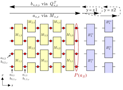
Figure 1: A square lattice picture of our model (with $S=5$ and $n=4$), which exhibits EmQM on a one-dimensional boundary (circled in red) of a two-dimensional bulk. Classical bits $a_{s,x}$ (red dots) propagate forward through a slowly time-evolving circuit of stochastic matrices $M_{s,x}$ (yellow), and classical bits $b_{s,x,\gamma}$ propagate backwards through a time-independent circuit of permutation matrices $Q_{s,x}^{T}$. The emergent Schrödinger equation describes the time evolution of the probability distribution $P(a_{S})$ governing the boundary bits. The back-propagating bits determine how the stochastic matrices are updated in each time step. See Sec. III.1 for an overview.

Simulating Schrödinger’s equation with a classical computer generically requires CPU time that increases exponentially with system size. Therefore, simulating an underlying classical EmQM model should also have a high cost. To ensure that the EmQM model is costly to simulate, we posit a large extra spatial dimension of length $S$. In effect, this large dimension enables the EmQM model to describe quantum mechanics in an exponentially large Hilbert space.

In our model, the stochastic classical bits are fast in the sense that they are frequently sampled. But the emergent wavefunction is related to the probability distribution $\bm{P}$ from which these bits are sampled, where $\bm{P}$ itself evolves quite slowly in comparison. A general probability distribution on $n$ bits is parameterized by $2^{n}-1$ nonnegative real numbers. If we want to allow general $n$-qubit quantum pure states in our EmQM model, then many parameters must be needed to specify the stochastic process from which $\bm{P}$ arises. For this reason we assume that $\bm{P}$ is obtained by composing stochastic matrices in a very deep circuit. The number of parameters needed to parameterize the circuit is linear in its depth $S$, which we therefore assume to be exponential in $n$. We envision this circuit as extending into an auxiliary spatial dimension, not to be confused with the spatial dimensions of the emergent quantum system.

Consider an EmQM model consisting of an $S+1$ by $n$ grid of bits $a_{s,x}$, which are depicted as red dots in Fig. 1. For simplicity of exposition, we focus on the EmQM of a one-dimensional chain of $n$ qubits. Generalizations to higher spatial dimensions are straightforward. Let $\bm{P}$ be the probability distribution for the $n$ bits at the $s=S$ boundary (circled in red) of the extra spatial dimension. We then suppose that at the $s=0$ boundary, the $n$ bits are generated uniformly at random, and that the bulk dynamics interpolate between the uniform distribution $\frac{\bm{1}}{N}$ and $\bm{P}=\frac{\bm{1}}{N}+\epsilon_{\Psi}\Psi$.

Next, we take inspiration from unitary circuits, which can generate entangled wavefunctions from direct product states by repeatedly acting on pairs of qubits with unitary matrices. Since the EmQM model involves classical bits instead of qubits, we instead consider a circuit of stochastic matrices $M_{s,x}$ (yellow in Fig. 1). A stochastic matrix is a matrix with columns that are probability vectors, i.e. vectors with positive entries that sum to one. Therefore, given two input bits, a $4\times 4$ stochastic matrix maps those bits to a probability distribution, from which a new pair of bits can be sampled. A $4\times 4$ stochastic matrix can also be used to linearly map a probability vector for two bits to a new probability vector. The EmQM model utilizes a circuit of stochastic matrices to sample bits from the probability vector $\bm{P}$. We emphasize that $\bm{P}$ is not a physical degree of freedom; $\bm{P}$ is only implicitly defined by the circuit of stochastic matrices.

The stochastic matrices $M_{s,x}$ vary slowly with the time step $\tau$, and can be decomposed as

$$M_{s,x}(\tau)=Q_{s,x}+m_{s,x}(\tau),$$ (5)

where $Q_{s,x}$ is time-independent and $m_{s,x}(\tau)$ is a time-dependent perturbation. We take the $Q_{s,x}$ to be permutation matrices, which have the useful property that their inverse is also a stochastic matrix. We will assume that at all times, the perturbation $m_{s,x}(\tau)$ is sufficiently small that we can accurately account for the evolution of $\bm{P}$ by expanding to linear order. As a result, the time evolution of the emergent wavefunction will also be described by a linear equation.

II.5 Unitarity from Destructive Interference

A final challenge is to obtain dynamics for $\bm{P}$ such that $\Psi$ in Eq. (2) undergoes a unitary evolution described by Schrödinger’s equation. One route to realizing unitarity is to suppose that after the forward-propagating bits $a_{s,x}$ reach the $s=S$ boundary, the bits are transformed by a shallow stochastic circuit $B$ that encodes a small unitary time evolution generated by the Hamiltonian $H$. The resulting bits could then back-propagate through the circuit (via $Q_{s,x}^{T}$) while dictating how the stochastic matrices slowly evolve such that $\bm{P}$ undergoes the desired dynamics.

But how could a stochastic circuit encode a time evolution by a generic imaginary-valued Hamiltonian satisfying Eq. (4)? One possibility is that a pair of stochastic circuits $B^{(\pm)}$ outputs two sets of bits with probability vectors $\bm{P}_{\pm}$ that “destructively interfere” with each other:

$$\bm{P}_{+}-\bm{P}_{-}=(-iH\delta_{\text{t}})\cdot\bm{P}$$ (6)

This could be achieved by stochastic circuits $B^{(\pm)}$ defined such that

$$B^{(+)}-B^{(-)}=-iH\delta_{\text{t}}$$ (7)

Such a decomposition is always possible for sufficiently small $\delta_{\text{t}}$. For example, if

$$-iH=\begin{pmatrix}0&-1&+1&0\\ +1&0&-1&0\\ -1&+1&0&0\\ 0&0&0&0\end{pmatrix}$$ (8)

for $n=2$ qubits, then we can choose

$$B^{(+)} =\begin{pmatrix}1-\delta_{\text{t}}&0&\delta_{\text{t}}&0\\ \delta_{\text{t}}&1-\delta_{\text{t}}&0&0\\ 0&\delta_{\text{t}}&1-\delta_{\text{t}}&0\\ 0&0&0&1\end{pmatrix}$$ (9)

$$B^{(-)} =\begin{pmatrix}1-\delta_{\text{t}}&\delta_{\text{t}}&0&0\\ 0&1-\delta_{\text{t}}&\delta_{\text{t}}&0\\ \delta_{\text{t}}&0&1-\delta_{\text{t}}&0\\ 0&0&0&1\end{pmatrix}$$

To illustrate how this works in a simple setting, let us continue this $n=2$ example and further suppose that $S=1$ such that there is only a single stochastic matrix $M$, as depicted below:

(10)

For each discrete time step, all of the bits $a_{s,x}$ and $b_{s,x,\pm}$ are updated. The two input bits $a_{0,1}$ and $a_{0,2}$ are chosen uniformly at random. The boundary bits at $s=1$ are randomly chosen from the conditional probability distributions $p(a_{1}|a_{0})=M(a_{1},a_{0})$ and $p(b_{\pm}|a_{1})=B^{(\pm)}(b_{\pm},a_{1})$, where (for now) $a_{s}$ and $b_{\pm}$ denote pairs of bits $(a_{s,1},a_{s,2})$ and $(b_{1,1,\pm},b_{1,2,\pm})$, which are used to index the $4\times 4$ matrices $M$ and $B^{(\pm)}$.

In order to get the desired time evolution for $\bm{P}$, for each discrete time step, $m$ in $M=Q+m$ is updated according to

$$m^{\prime}=m+\Delta_{\text{m}}(\bm{\hat{b}}_{+}-\bm{\hat{b}}_{-})\otimes\bm{\hat{e}}$$ (11)

where $\Delta_{\text{m}}$ is a small constant. $\bm{\hat{b}}_{+}$ denotes the basis 4-vector indexed by the two bits $b_{1,1,+}$ and $b_{1,2,+}$, and similar for $\bm{\hat{b}}_{-}$. For example, $\bm{\hat{b}}_{+}=(0,1,0,0)$ if $b_{1,1,+}=0$ and $b_{1,2,+}=1$. $\bm{\hat{e}}$ is chosen uniformly at random from the four basis 4-vectors [$(1,0,0,0)$, $(0,1,0,0)$, etc.] with the constraint that $M=Q+m$ remains non-negative. Such a choice always exists as long as the elements of $m$ (which are assumed to be small) remain smaller than 1. The choice of $Q$ does not play an important role in this $S=1$ example.

$\bm{P}$ is the probability distribution that governs the sampled boundary bits $a_{1,1}$ and $a_{1,2}$. In addition, $\bm{P}$ itself has statistical fluctuations, because in each time step, the stochastic matrix $M$ is updated according to Eq. (11), where $\bm{\hat{b}}_{+}$ and $\bm{\hat{b}}_{-}$ are also stochastic variables. To see that Eq. (11) results in an emergent Schrödinger equation, we first calculate the expectation values (denoted by a bar) of the boundary bits:

$$\bm{P}=\overline{\bm{\hat{a}}_{1}} =M\cdot\frac{\bm{1}_{4}}{4}$$ (12)

$$\overline{\bm{\hat{b}}_{\pm}} =B^{(\pm)}\cdot\bm{P}$$ (13)

where $\bm{1}_{4}/4$ denotes a uniform probability vector with 4 elements. Eq. (7) then implies that

$$\overline{\bm{\hat{b}}_{+}-\bm{\hat{b}}_{-}}=-i\delta_{\text{t}}H\cdot\bm{P}$$ (14)

Thus, the average change in $\bm{P}$ after one time step evolves according to a discrete Schrödinger’s equation:

$$\overline{\bm{P}^{\prime}-\bm{P}} =\left(\overline{m^{\prime}-m}\right)\cdot\frac{\bm{1}_{4}}{4}$$ (15)

$$=\frac{\Delta_{\text{m}}}{4}\left(\overline{\bm{\hat{b}}_{+}-\bm{\hat{b}}_{-}}\right)$$

$$=-i\Delta_{\text{t}}H\cdot\bm{P}$$

where $\Delta_{\text{t}}=\frac{1}{4}\delta_{\text{t}}\Delta_{\text{m}}$. The above three equalities follow from Eqs. (12), (11), and (14), respectively. In the second equality, we see that the random choice of $\bm{\hat{e}}$ in Eq. (11) does not matter because $\bm{\hat{e}}$ is multiplied by $\bm{1}_{4}$ in the first line. Since $\bm{P}$ and $\Psi$ are linearly related by Eq. (2), $\Psi$ obeys Schrödinger’s equation on average. Statistical fluctuations about this average are negligible in the small $\Delta_{\text{m}}$ limit.

To quantify statistical fluctuations, let $\tau$ denote the discrete time step of $\bm{P}^{(\tau)}$. After $\tau$ steps, the elapsed time in the emergent quantum mechanics is $t\approx\Delta_{\text{t}}\tau$. Statistical fluctuations of $\bm{P}^{(\tau)}$ grow as $O(\Delta_{\text{m}}\sqrt{\delta_{t}\tau})=O(\sqrt{\Delta_{\text{m}}t})$. Therefore, statistical fluctuations become arbitrarily small as $\Delta_{\text{m}}$ decreases.

II.6 More Qubits

Finally, we must scale up the previous $S=1$ and $n=2$ example to large $S$ and $n$, as depicted in Fig. 1. We will now assume that the time-independent permutation matrices $Q_{s,x}$ in Eq. (5) are chosen uniformly at random and independently for each $s$ and $x$. These random permutation matrices play an important role as they randomize the subspace in which each $m_{s,x}$ affects $\bm{P}$. Therefore when $Sn\gg N=2^{n}$, the span of these subspaces covers all $N$ dimensions of $\bm{P}$.

When $S>1$, the bits $b_{S,x,\gamma}$ at the boundary will have to back-propagate through the circuit before affecting the time evolution of $M_{s,x}$. In order to back-propagate the maximal amount of information from the boundary to the bulk, it would be ideal to use the inverse of the stochastic matrices $M_{s,x}^{-1}$. But this is not possible since these inverses are generically not stochastic matrices. However, since $m_{s,x}$ is assumed to be small, $M_{s,x}^{-1}\approx Q_{s,x}^{T}$ and therefore $Q_{s,x}^{T}$ can be used to deterministically back-propagate the bits.

Finally, we must split $B^{(\pm)}$ into local pieces, as depicted in Fig. 1. To be concrete, we assume that the Hamiltonian $H=\sum_{x}H_{x}$ is local such that each $H_{x}$ only acts on two neighboring qubits. Generalizing Eq. (7), $B_{x}^{(\pm)}$ are chosen such that

$$B_{x}^{(+)}-B_{x}^{(-)}=-iH_{x}\delta_{\text{t}}$$ (16)

with the constraint that the stochastic matrix

$$B_{x}^{(\pm)}=\mathbbl{1}_{4}+O(\delta_{\text{t}})$$ (17)

is the $4\times 4$ identity matrix $\mathbbl{1}_{4}$ up to order $\delta_{\text{t}}$ corrections. We then define four different depth-1 stochastic circuits:

$$B^{(\pm 1)} =\operatorname*{\text{\scalebox{1.2}{$\otimes$}}}_{\text{odd }x}B_{x}^{(\pm)}$$ (18)

$$B^{(\pm 2)} =\operatorname*{\text{\scalebox{1.2}{$\otimes$}}}_{\text{even }x}B_{x}^{(\pm)}$$

which are now guaranteed to satisfy a generalization of Eq. (7):

$$+B^{(+1)}-B^{(-1)}+B^{(+2)}-B^{(-2)}=-iH\delta_{\text{t}}+O(\delta_{\text{t}}^{2})$$ (19)

Since there are now four different flavors of $B^{(\gamma)}$, we also take four different flavors of back-propagating bits $b_{s,x,\gamma}$ with $\gamma=\pm 1$ and $\gamma=\pm 2$. With these ingredients combined, we arrive at a local model of emergent quantum mechanics.

III EmQM Model

III.1 Overview

In summary, we introduce a two-dimensional local classical model for which a wavefunction $\Psi$ of qubits is encoded in a probability distribution $\bm{P}=\frac{\bm{1}}{N}+\epsilon_{\Psi}\Psi$ [Eq. (2)] for $n$ classical bits on a one-dimensional boundary of the model. Generalizing to higher dimensions or $Z_{k}$ qudits (rather than $Z_{2}$ qubits) is straightforward. For each discrete time step, a bit string $a_{S}$ (e.g. $a_{S}=011010$) is generated with probability $P(a_{S})$ at the $s=S$ boundary. Our model exhibits EmQM in the sense that $\bm{P}$ [i.e. $P(a_{S})$ viewed as a vector with $N=2^{n}$ components] evolves according to

$$\partial_{t}\bm{P}\approx-iH\cdot\bm{P}$$ (20)

where $H$ is imaginary-valued and obeys Eq. (4). Schrödinger’s equation (1) for $\Psi$ then follows from $\bm{P}=\frac{\bm{1}}{N}+\epsilon_{\Psi}\Psi$ [Eq. (2)]. We will derive Eq. (20) from a well-controlled perturbation theory, which we verify numerically. Furthermore, the approximate equality in Eq. (20) becomes exact in a well-defined limit.

variable	definition	reference
$n$	number of bits output by circuit at each time step	Sec. III.1
$N=2^{n}$	number of bit strings for $n$ bits; $x=1,2,\ldots,n$	Sec. III.1
$S$	length of extra dimension; $s=1,2,\ldots,S$	Sec. III.1
$\delta_{\text{t}}$	raw time step (not to be confused with $\Delta_{\text{t}}$)	Sec. II.5
$m_{0}$	approximate Hilbert–Schmidt norm of each $m_{s,x}$	Eq. (28)
$\Delta_{\text{m}}$	step size for $m_{s,x}$ for each time step	Eq. (31)
$\epsilon_{0}$	small parameter used to parameterize the above four constants	Eq. (79)
$H$, $H_{x}$	effective local Hamiltonian $H=\sum_{x}H_{x}$	Sec. III.1
$G$, $G_{x}$	real-valued: $G=-iH$, $G_{x}=-iH_{x}$	Eq. (36)
$\Delta_{\text{t}}$	effective EmQM time step: $t\approx\Delta_{t}\tau$	Eq. (50)
$\epsilon_{\Psi}$	small constant relating $\bm{P}-\frac{\bm{1}}{N}\approx\epsilon_{\Psi}\Psi$	Eqs. (2) and (54)
$B_{x}^{(\pm)}$	$4\times 4$ stochastic matrix used to sample $b_{s,x,\pm\gamma}$	Eqs. (16), (29), and (37)
$B^{(\gamma)}$	depth-1 stochastic circuit; related to Hamiltonian	Eqs. (18) and (19)
$\Delta_{\text{P}}$	rough 2-norm of $\overline{\bm{P}^{(\tau)}-\bm{P}^{(\tau-1)}}$	Eq. (53)
$P(a_{S})$	probability the circuit outputs bit string $a_{S}$	Sec. III.1
$\bm{P}=\bm{P}_{S}$	expectation value of $\bm{\hat{a}}_{S}$, or $P(a_{S})$ viewed as a probability vector	Eqs. (23), and (28)
$\varepsilon(t)$	EmQM deviation $||\Psi(t)-\Psi_{\text{QM}}(t)||$ from quantum mechanics (QM)	Eqs. (52) and (75)
$\varepsilon_{\text{m}}(t)$, $\varepsilon_{\text{t}}(t)$	deviations due to finite $m_{0}$ and $\delta_{\text{t}}$	Eqs. (63) and (65)
$\varepsilon_{\text{S}}(t)$, $\varepsilon_{\text{stat}}(t)$	deviations due to finite $S$ and statistical fluctuations	Eqs. (70) and (74)
$\tau$	integer-valued time step	Sec. III.2
$a_{s,x}$	a forward-propagating stochastic bit	Sec. III.1
$a_{s,\mathbbl{x}}$	pair of bits $(a_{s,x},a_{s,x+1})$	above Eq. (21)
$a_{s}$	bit string ($a_{s,1},a_{s,2},\ldots,a_{s,n}$)	below Eq. (22)
$\bm{\hat{a}}_{s}$	length-$n$ basis vector indexed by the bit string $a_{s}$	below Eq. (39)
$b_{s,x,\gamma}$	a backward-propagating stochastic bit	Sec. III.1
$b_{s,\mathbbl{x},\gamma}$	a pair of bits $(b_{s,x,\gamma},a_{s,x+1,\gamma})$	above Eq. (29)
$\bm{\hat{b}}_{s,\mathbbl{x},\gamma}$	$(1,0,0,0)$, $(0,1,0,0)$, $(0,0,1,0)$, or $(0,0,0,1)$ when $b_{s,\mathbbl{x},\gamma}=00$, $01$, $10$, or $11$	below Eq. (34)
$b_{s,\gamma}$	bit string $(b_{s,1,\gamma},b_{s,2,\gamma},\ldots,b_{s,n,\gamma})$	below Eq. (34)
$\bm{\hat{b}}_{s,\gamma}$	length-$n$ basis vector indexed by the bit string $b_{s,\gamma}$	below Eq. (34)
$M_{s,x}$	$4\times 4$ stochastic matrices, which define the classical circuit	Sec. III.1
$M_{s}$	Kronecker product of $M_{s,x}$ with fixed $s$	Eq. (24)
$M_{S\leftarrow s}$	$=M_{S}\cdot M_{S-1}\cdots M_{s+1}$	Eq. (56)
$m_{s,x}$	perturbations to $M_{s,x}=Q_{s,x}+m_{s,x}$	Eq. (25)
$Q_{s,x}$	time-independent $4\times 4$ permutation matrices	below Eq. (25)
$Q_{s}$	Kronecker product of $Q_{s,x}$ with fixed $s$	Eq. (26)
$Q_{S\leftarrow s}$	$=Q_{S}\cdot Q_{S-1}\cdots Q_{s+1}$	Eq. (27)
$\bm{1}$ or $\bm{1}_{n}$	vector of $n$ ones
$\mathbbl{1}$ or $\mathbbl{1}_{n}$	$n\times n$ identity matrix
$\mathcal{P}_{x}$	projects out all bits except $x$ and $x+1$	Eq. (35)
$\mathcal{W}$	sum of conjugated projectors $\mathcal{P}_{x}$	Eqs. (66) and (44)

Table 1: A table of notation used throughout the main text [with the exception of Sec. II.5 which uses some simplified notations]. Notations are grouped as follows: model parameters, dependent variables, dynamical variables, randomly-initialized constants, and other constants.

Fig. 1 summarizes the basic structure of our EmQM model. The model consists of a square lattice of classical bits $a_{s,x}$ and $b_{s,x,\gamma}$ (red dots) that propagate through a brick circuit of slowly-varying stochastic matrices $M_{s,x}$ (yellow). For each discrete time step, pairs of classical forward-propagating bits ($a_{s,x}$ and $a_{s,x+1}$) are randomly sampled (21) from probability distributions conditioned on the pair of bits to the left ($a_{s-1,x}$ and $a_{s-1,x-1}$). The conditional probabilities are encoded in the stochastic matrices $M_{s,x}$, which are perturbatively close to time-independent permutation matrices $Q_{s,x}\approx M_{s,x}$. Also at each time step, pairs of backward-propagating bits ($b_{s,x,\gamma}$ and $b_{s,x+1,\gamma}$) are deterministically replaced (30) by the permutation $Q_{s,x}^{T}$ of bits to their right ($b_{s+1,x}$ and $b_{s+1,x+1}$). The bits $a_{0,x}$ at the left $s=0$ boundary are uniformly initialized at random. The bits $b_{S,x,\gamma}$ at the right $s=S$ boundary result from applying (29) a shallow stochastic circuit (18) to the bits $a_{S,x}$ at $s=S$. The shallow circuit is related (19) to the Hamiltonian and consists of a layer of time-independent stochastic matrices $B_{x}^{(\pm)}$ (blue). The bits $a_{S,x}$ on the $s=S$ boundary (circled in red) follow a probability distribution $\bm{P}$ defined by a tensor network product (23) of the matrices $M_{s,x}$. The time-evolution of $M_{s,x}$ depends (31) on back-propagating bits $b_{s,x,\gamma}$, which effectively back-propagate the result of a small Hamiltonian time evolution on $\bm{P}$, such that $\bm{P}$ and $\Psi$ approximately obey Schrödinger’s equation. See Tab. 1 for a notational reference.

III.2 Stochastic Circuit

We now define and study the EmQM model in greater detail. Each lattice site hosts a classical bit $a_{s,x}=0,1$, where $s=0,1,\ldots,S$, and $x=1,\ldots,n$ index the different lattice sites. $s$ is the coordinate for an extra dimension, while $x$ is the coordinate for the spatial dimension on which the emergent qubits live. Our model evolves in discrete time steps indexed by integer-valued $\tau$, while $t$ is reserved for the emergent time variable of the emergent quantum mechanics. $a_{s,x}^{(\tau)}$ denotes the value of the bit $a_{s,x}$ at time step $\tau$, and similar for other time-dependent variables. In contexts where the time step is not important, we often omit the $(\tau)$ superscript to avoid clutter.

To avoid clutter, we denote a pair of bits $(a_{s,x},a_{s,x+1})$ as $a_{s,\mathbbl{x}}$, where $\mathbbl{x}$ is shorthand for $(x,x+1)$. For each time step $\tau$, the classical bits $a_{s,x}^{(\tau-1)}$ with $1\leq s\leq S$ are stochastically updated to $a_{s,x}^{(\tau)}$ with conditional probabilities that are conditioned on the bits $a_{s-1,\mathbbl{x}}^{(\tau-1)}$. These conditional probabilities are given by time-dependent stochastic matrices $M_{s,x}$:

$$p(a_{s,\mathbbl{x}}^{(\tau)}|a_{s-1,\mathbbl{x}}^{(\tau-1)})=M_{s,x}^{(\tau-1)}(a_{s,\mathbbl{x}}^{(\tau)},a_{s-1,\mathbbl{x}}^{(\tau-1)})$$ (21)

For each $(s,x)$ with $s=1,2,\ldots,S$ and $s-x$ even, $M_{s,x}$ is a $4\times 4$ stochastic matrix. That is, the columns of $M_{s,x}$ are probability vectors; i.e. $M_{s,x}$ has positive elements and columns that sum to 1. We index the $4\times 4$ matrices using pairs of bits, such that for fixed $a_{s-1,\mathbbl{x}}^{(\tau-1)}$, $M_{s,x}^{(\tau-1)}(a_{s,\mathbbl{x}}^{(\tau)},a_{s-1,\mathbbl{x}}^{(\tau-1)})$ is a probability distribution for $a_{s,\mathbbl{x}}^{(\tau)}$. The bits along the $s=0$ line at the beginning of the circuit are randomly sampled with equal probability:

$$p(a_{0,x})=1/2$$ (22)

Let $a_{s}\equiv(a_{s,1},a_{s,2},\ldots,a_{s,n})$ denote the string of bits along a column of fixed $s$. For each $s$, let $\bm{P}_{s}$ denote the vector of probabilities for the different bit strings $a_{s}$. Then $\bm{P}_{s}^{(\tau)}$ can be expressed recursively as

$$\bm{P}_{s}^{(\tau)} =M_{s}^{(\tau-1)}\cdot\bm{P}_{s-1}^{(\tau-1)}$$ (23)

$$\bm{P}_{0}^{(\tau)} =\frac{\bm{1}}{N}$$

where $M_{s}$ denotes the Kronecker product of stochastic matrices with fixed $s$:

$$M_{s}^{(\tau)}=\operatorname*{\text{\scalebox{1.2}{$\otimes$}}}_{x}^{\begin{subarray}{c}\text{even}\\ s-x\end{subarray}}M_{s,x}^{(\tau)}.$$ (24)

The notation on the right-hand side means we take the Kronecker product of all $M_{s,x}^{(\tau)}$ for even $x$ when $s$ is even (or for odd $x$ when $s$ is odd), producing the brickwork circuit shown in Fig. 1. The bit string probabilities at the end of the circuit are given by $\bm{P}=\bm{P}_{S}$ (circled in red in Fig. 1).

III.3 Perturbative Expansion

To gain analytical tractability, we assume that the stochastic matrices are very close to permutation matrices:

$$M_{s,x}^{(\tau)}=Q_{s,x}+m_{s,x}^{(\tau)}$$ (25)

Each $Q_{s,x}$ is a randomly-chosen (for each $s$ and $x$) but time-independent $4\times 4$ permutation matrix, while $m_{s,x}^{(\tau)}$ is a small time-dependent perturbation. A permutation matrix is a stochastic matrix where all elements are either 0 or 1. A matrix is a permutation matrix if and only if it is both stochastic and orthogonal. The dynamics of $m_{s,x}$ will be constrained such that $M_{s,x}$ remains a stochastic matrix (with non-negative components).

Since they are orthogonal, the permutation matrices have the effect of a basis transformation. Similar to Eq. (24), let $Q_{s}$ denote the Kronecker product of permutation matrices with fixed $s$:

$$Q_{s}=\operatorname*{\text{\scalebox{1.2}{$\otimes$}}}_{x}^{\begin{subarray}{c}\text{even}\\ s-x\end{subarray}}Q_{s,x}$$ (26)

Let $Q_{S\leftarrow s}$ denote the product

$$Q_{S\leftarrow s}=Q_{S}\cdot Q_{S-1}\cdots Q_{s+1}$$ (27)

such that it encodes the change of basis from the column of bits at $s$ to the end at $s=S$.

Expanding $\bm{P}$ to first order in the perturbations $m_{s,x}$ results in:

$$\bm{P}^{(\tau)}=\frac{\bm{1}}{N}+\sum_{s=1}^{S}\sum_{x}^{\begin{subarray}{c}\text{even}\\ s-x\end{subarray}}Q_{S\leftarrow s}\cdot m_{s,x}^{(\tau_{s})}\cdot\frac{\bm{1}}{N}+O(m_{0}^{2})$$ (28)

where $\tau_{s}=\tau-1-(S-s)$ results from a time delay, and $O(m_{0}^{2})$ denotes terms that are quadratic in $m_{s,x}$. For simplicity, we assume that each $m_{s,x}$ has Hilbert–Schmidt norm roughly equal to $m_{0}$. In Sec. IV, we will address more precisely the effects of the non-linear $O(m_{0}^{2})$ terms and other approximations that we make.

As elucidated in the above picture, $m_{s,x}^{(\tau_{s})}$ affects the probabilities for two bits at $s$ and $(x,x+1)$; these probabilities span a 4-dimensional subspace of the $N$-dimensional vector space of probabilities $\bm{P}_{s}$ (after averaging over the uniform distribution of input bits). This subspace is then scrambled into a different basis by the product $Q_{S\leftarrow s}$ of many random (but time-independent) permutation matrices. If $nS\gg N=2^{n}$, then the linear combination of these subspaces will span the entire $N$-dimensional vector space. Thus, the sum of contributions from all $m_{s,x}$ can encode any wavefunction $\Psi$ [that is real-valued and satisfies Eq. (3)], where $\bm{P}=\frac{\bm{1}}{N}+\epsilon_{\Psi}\Psi$ [Eq. (2)].

III.4 Time Evolution

We now want to give the perturbations $m_{s,x}$ a time evolution that leads to an emergent Schrödinger equation; i.e. $\bm{P}^{(\tau)}-\bm{P}^{(\tau-1)}\propto-iH\cdot\bm{P}$. To accomplish this, we introduce a set of backward-propagating bits $b_{s,x,\gamma}$ with $\gamma=\pm 1,\pm 2$. At the $s=S$ boundary, the pair of bits $b_{S,\mathbbl{x},\pm\gamma}^{(\tau)}$ are randomly sampled with probabilities that are conditioned on the bits $a_{S,\mathbbl{x}}^{(\tau-1)}$. These conditional probabilities are encoded in time-independent $4\times 4$ stochastic matrices $B_{x}^{(\pm)}$ (blue in Fig. 1):

$$p(b_{S,\mathbbl{x},\pm\gamma}^{(\tau)}|a_{S,\mathbbl{x}}^{(\tau-1)})=B_{x}^{(\pm)}(b_{S,\mathbbl{x},\pm\gamma}^{(\tau)},a_{S,\mathbbl{x}}^{(\tau-1)})$$ (29)

where $\gamma=1$ if $x$ is odd, else $\gamma=2$.

The bits $b_{s,\mathbbl{x},\gamma}$ deterministically propagate backwards through the circuit via the transposed permutation matrices $Q_{s,x}^{T}$:

$$\bm{\hat{b}}_{s,\mathbbl{x},\gamma}^{(\tau)}=Q_{s,x}^{T}\cdot\bm{\hat{b}}_{s+1,\mathbbl{x},\gamma}^{(\tau-1)}$$ (30)

The hat over $\bm{\hat{b}}_{s,\mathbbl{x},\gamma}^{(\tau)}$ denotes the basis 4-vector indexed by the two bits $b_{s,\mathbbl{x},\gamma}^{(\tau)}$; i.e. $\bm{\hat{b}}_{s,\mathbbl{x},\gamma}^{(\tau)}=(1,0,0,0)$ if $b_{s,\mathbbl{x},\gamma}^{(\tau)}=00$, and $\bm{\hat{b}}_{s,\mathbbl{x},\gamma}^{(\tau)}=(0,1,0,0)$ if $b_{s,\mathbbl{x},\gamma}^{(\tau)}=01$, etc.

The time-evolution of the perturbations $m_{s,x}$ is stochastic and depends on the back-propagating bits as follows [extending Eq. (11)]:

$$m_{s,x}^{(\tau)}=m_{s,x}^{(\tau-1)}+\Delta_{\text{m}}\sum_{\gamma=1,2}\left(\bm{\hat{b}}_{s,\mathbbl{x},+\gamma}^{(\tau)}-\bm{\hat{b}}_{s,\mathbbl{x},-\gamma}^{(\tau)}\right)\otimes\bm{\hat{e}}_{s-1,x,\gamma}^{(\tau)}$$ (31)

where $\Delta_{\text{m}}$ is a small positive constant. Similar to $\bm{\hat{b}}_{s,\mathbbl{x},\gamma}^{(\tau)}$ (defined in the previous paragraph), $\bm{\hat{e}}_{s-1,x,\gamma}^{(\tau)}$ is also one of the four basis 4-vectors, except it is chosen uniformly at random from the set of basis 4-vectors that keep $M_{s,x}^{(\tau)}=Q_{s,x}+m_{s,x}^{(\tau)}$ non-negative. Such a choice always exists as long as the elements of $m_{s,x}^{(\tau)}$ (which are assumed to be small) remain smaller than 1. The random choice of $\bm{\hat{e}}_{s-1,x,\gamma}^{(\tau)}$ has little effect since $m_{s,x}^{(\tau)}$ enters Eq. (28) after right-multiplication by $\bm{1}$.

The following quantity will play an important role:

$$\left(m_{s,x}^{(\tau)}-m_{s,x}^{(\tau-1)}\right)\cdot\frac{\bm{1}_{4}}{4}=\frac{\Delta_{\text{m}}}{4}\sum_{\gamma=1,2}\left(\bm{\hat{b}}_{s,\mathbbl{x},+\gamma}^{(\tau)}-\bm{\hat{b}}_{s,\mathbbl{x},-\gamma}^{(\tau)}\right)$$ (32)

where $\frac{\bm{1}_{4}}{4}$ is a length-4 uniform probability vector. When $m_{s,x}^{(\tau)}-m_{s,x}^{(\tau-1)}$ acts on two bits of a uniform probability vector of length $N=2^{n}$, the result is similar:

$$\left(m_{s,x}^{(\tau)}-m_{s,x}^{(\tau-1)}\right)\cdot\frac{\bm{1}_{N}}{N}$$

$$\quad=\frac{\bm{1}_{2^{x-1}}}{2^{x-1}}\otimes\left[\left(m_{s,x}^{(\tau)}-m_{s,x}^{(\tau-1)}\right)\cdot\frac{\bm{1}_{4}}{4}\right]\otimes\frac{\bm{1}_{2^{n-x-1}}}{2^{n-x-1}}$$ (33)

$$\quad=\frac{\Delta_{\text{m}}}{4}\sum_{\gamma=1,2}\mathcal{P}_{x}\cdot\left(\bm{\hat{b}}_{s,+\gamma}^{(\tau)}-\bm{\hat{b}}_{s,-\gamma}^{(\tau)}\right)$$ (34)

In the last line, $\bm{\hat{b}}_{s,\gamma}$ denotes a length-$n$ basis vector indexed by the bit string $b_{s,\gamma}=(b_{s,1,\gamma},b_{s,2,\gamma},\ldots,b_{s,n,\gamma})$. For example if $n=3$, then $\bm{\hat{b}}_{s,\gamma}=(1,0,0,0,0,0,0,0)$ if $b_{s,\gamma}=000$, and $\bm{\hat{b}}_{s,\gamma}=(0,1,0,0,0,0,0,0)$ if $b_{s,\gamma}=001$, etc. $m_{s,x}^{(\tau)}-m_{s,x}^{(\tau-1)}$ only acts on bits $x$ and $x+1$. Therefore the other bits are projected out by the projection matrix

$$\mathcal{P}_{x}=\operatorname*{\text{\scalebox{1.2}{$\otimes$}}}_{x^{\prime}=1}^{n}\begin{cases}\quad\begin{pmatrix}1&0\\ 0&1\end{pmatrix}&\text{\parbox[c][0.0pt][t]{39.0242pt}{$x^{\prime}=x\;$ or \\ $x^{\prime}=x+1$}}\\ \begin{pmatrix}1/2&1/2\\ 1/2&1/2\end{pmatrix}&\text{otherwise}\end{cases}$$ (35)

Expressing Eq. (34) in this way will be useful later on.

III.5 $B_{x}^{(\pm)}$ Encode the Hamiltonian

Given a Hamiltonian $H=\sum_{x}H_{x}$, we now wish to choose $B_{x}^{(\pm)}$ such that inserting Eq. (34) into (28) yields a discrete Schrödinger equation: $\bm{P}^{(\tau)}-\bm{P}^{(\tau-1)}\propto G\cdot\bm{P}$ where we define

$$G=-iH$$ (36)

and $G_{x}=-iH_{x}$.

We assume $H_{x}$ is Hermitian, imaginary-valued, and acts only on two neighboring qubits, which implies that $G_{x}$ is a real antisymmetric $4\times 4$ matrix. In accordance with Eq. (4), we further assume that $G_{x}$ has rows and columns that sum to zero. We also decompose $G_{x}=G_{x}^{(+)}-G_{x}^{(-)}$ such that $G_{x}^{(+)}$ and $G_{x}^{(-)}$ only have non-negative elements.

We require that $B_{x}^{(\pm)}$ satisfy Eqs. (16) and (17) so that these matrices encode the Hamiltonian, as in Eq. (19). To achieve this for a general (geometrically two-local) Hamiltonian, we choose $B_{x}^{(\pm)}$ to be the following $4\times 4$ matrix:

$$B_{x}^{(\pm)}(b_{\pm},a) =\delta_{\text{t}}G_{x}^{(\pm)}(b_{\pm},a)$$ (37)

$$\quad+\begin{cases}1-\delta_{\text{t}}\,g_{x}(a)&b_{\pm}=a\\ 0&b_{\pm}\neq a\end{cases}$$

where $g_{x}(a)$ is a column sum of $G_{x}^{(\pm)}$:

$$g_{x}(a)=\sum_{b=00,01,10,11}\,G_{x}^{(\pm)}(b,a)$$ (38)

“$b_{+}$”, “$b_{-}$”, and “$a$” each denote a pair of bits, which respectively correspond to $b_{S,\mathbbl{x},+\gamma}$, $b_{S,\mathbbl{x},-\gamma}$, and $a_{S,\mathbbl{x}}$ in Eq. (29). $B_{x}^{(\pm)}$ are $4\times 4$ stochastic matrices, which we view as a probability vector for 2 bits ($b_{\pm}$) given two bits ($a$). Either $G_{x}^{(+)}$ or $G_{x}^{(-)}$ can be used in the right-hand-side of Eq. (38); both give the same result since the column sum of $G_{x}=G_{x}^{(+)}-G_{x}^{(-)}$ is zero. $B_{x}^{(\pm)}$ is a stochastic matrix as long as $\delta_{\text{t}}$ is sufficiently small. See Eq. (9) for an example.

Importantly, since this choice of $B_{x}^{(\pm)}$ implies Eq. (19), the bits $b_{S,\gamma}$ encode a short time evolution by the Hamiltonian:

$$\sum_{\gamma=1,2}\overline{\bm{\hat{b}}_{S,+\gamma}^{(\tau)}-\bm{\hat{b}}_{S,-\gamma}^{(\tau)}}$$

$$\quad=(+B^{(+1)}-B^{(-1)}+B^{(+2)}-B^{(-2)})\cdot\overline{\bm{\hat{a}}_{S}^{(\tau-1)}}$$

$$\quad=(-i\delta_{\text{t}}H)\cdot\bm{P}^{(\tau-1)}+O(\delta_{\text{t}}^{2})$$ (39)

The first equality follows from Eq. (29), where $B^{(\gamma)}$ was defined in Eq. (18). Similar to the $\bm{\hat{b}}_{s,\gamma}$ notation, $\bm{\hat{a}}_{s}$ denotes a length-$n$ basis vector indexed by the bit string $a_{s}$. The final line follows from Eq. (19) and the definition $\bm{P}^{(\tau)}=\overline{\bm{\hat{a}}_{S}^{(\tau)}}$.

III.6 Emergent Quantum Mechanics

Now that we have specified the EmQM model, we show that it can exhibit emergent quantum mechanics. We begin by evaluating the expectation value of $\bm{P}^{(\tau)}-\bm{P}^{(\tau-1)}$ using Eq. (28):

$$\overline{\bm{P}^{(\tau)}-\bm{P}^{(\tau-1)}}=$$ (40)

$$\quad\sum_{s=1}^{S}\sum_{x}^{\begin{subarray}{c}\text{even}\\ s-x\end{subarray}}Q_{S\leftarrow s}\cdot\left(\overline{m_{s,x}^{(\tau_{s})}-m_{s,x}^{(\tau_{s}-1)}}\right)\cdot\frac{\bm{1}}{N}+O(m_{0}^{2})$$

We can simplify the summand as follows:

$$\left(\overline{m_{s,x}^{(\tau_{s})}-m_{s,x}^{(\tau_{s}-1)}}\right)\cdot\frac{\bm{1}}{N}$$

$$\quad=\frac{\Delta_{\text{m}}}{4}\sum_{\gamma=1,2}\mathcal{P}_{x}\cdot Q_{S\leftarrow s}^{T}\cdot\left(\overline{\bm{\hat{b}}_{S,+\gamma}^{(\tau_{s}^{\prime})}-\bm{\hat{b}}_{S,-\gamma}^{(\tau_{s}^{\prime})}}\right)$$ (41)

$$\quad=\frac{\Delta_{\text{m}}}{4}\mathcal{P}_{x}\cdot Q_{S\leftarrow s}^{T}\cdot(-i\delta_{\text{t}}H)\cdot\overline{\bm{P}^{(\tau_{s}^{\prime}-1)}}+O(\delta_{\text{t}}^{2})$$ (42)

Eq. (41) is obtained from Eq. (34) after replacing $\bm{\hat{b}}_{s,\gamma}^{(\tau_{s})}=Q_{S\leftarrow s}^{T}\cdot\bm{\hat{b}}_{S,\gamma}^{(\tau_{s}^{\prime})}$, where $\tau_{s}^{\prime}=\tau_{s}-(S-s)=\tau-1-2(S-s)$. Eq. (42) follows from Eq. (39).

We assume $\Delta_{\text{m}}\ll S^{-1}$ such that the slow variables $m_{s,x}$ change very little over $S$ time steps so that we can approximate $\bm{P}^{(\tau_{s}^{\prime}-1)}=\bm{P}^{(\tau-1)}+O(S\Delta_{\text{m}})$. Inserting Eq. (42) into (40) results in

$$\overline{\bm{P}^{(\tau)}-\bm{P}^{(\tau-1)}} =\frac{\Delta_{\text{m}}}{4}\delta_{\text{t}}\,\mathcal{W}\cdot(-iH)\cdot\overline{\bm{P}^{(\tau-1)}}$$ (43)

$$\quad+O(m_{0}^{2},\delta_{\text{t}}^{2},\Delta_{\text{m}}^{2})$$

where $\mathcal{W}$ is a sum of conjugated projectors $\mathcal{P}_{x}$ [Eq. (35)]:

$$\mathcal{W}=\sum_{s=1}^{S}\sum_{x}^{\begin{subarray}{c}\text{even}\\ s-x\end{subarray}}Q_{S\leftarrow s}\cdot\mathcal{P}_{x}\cdot Q_{S\leftarrow s}^{T}$$ (44)

The error estimates $O(m_{0}^{2},\delta_{\text{t}}^{2},\Delta_{\text{m}}^{2})$ in Eq. (43) neglect factors of $S$ and $N$, which will be accounted for in Sec. IV.

If $Sn\gg N$, then $\mathcal{W}$ approaches a simple form:

$$\mathcal{W}=\underbrace{\frac{Sn}{2}\mathcal{P}_{\bm{1}}+\frac{Sn}{2}\frac{3}{N-1}\mathcal{P}_{\bm{1}}^{\perp}}_{\mathcal{W}_{0}}+O\!\left(\sqrt{\frac{Sn}{N}}\right)$$ (45)

where the matrix $\mathcal{P}_{\bm{1}}=\frac{\bm{1}\otimes\bm{1}}{N}$ projects onto the one-dimensional subspace spanned by $\bm{1}$ (i.e. the vector of $N$ ones) and $\mathcal{P}_{\bm{1}}^{\perp}=\mathbbl{1}-\mathcal{P}_{\bm{1}}$ projects into the orthogonal subspace. $\mathbbl{1}$ is an $N\times N$ identity matrix.

The first term in Eq. (45) follows from multiplying Eq. (44) by $\bm{1}$, and noting that $Sn/2$ is the number of terms summed in Eq. (44). To understand the following two terms, note that within the $(N-1)$-dimensional subspace orthogonal to $\bm{1}$, the set of permutation matrices is a unitary 1-design Dankert et al. (2009) up to a constant factor. That is,

$$\operatorname*{\text{\scalebox{1.2}{$\mathbb{E}$}}}_{Q}\;Q_{\perp}\otimes Q_{\perp}^{T}=\frac{1}{1-N^{-1}}\operatorname*{\text{\scalebox{1.2}{$\mathbb{E}$}}}_{U}\;U_{\perp}\otimes U_{\perp}^{\dagger}$$ (46)

where $Q_{\perp}=\mathcal{P}_{\bm{1}}^{\perp}\cdot Q\cdot\mathcal{P}_{\bm{1}}^{\perp}$ and $U_{\perp}=\mathcal{P}_{\bm{1}}^{\perp}\cdot U\cdot\mathcal{P}_{\bm{1}}^{\perp}$, and $\operatorname*{\mathbb{E}}_{Q}$ averages over all permutation matrices $Q$ while $\operatorname*{\mathbb{E}}_{U}$ averages over all unitary matrices. Our numerical experiments show that the permutation matrices $Q_{S\leftarrow s}$ with $S-s\gg n$ summed in Eq. (44) are an approximate 1-design in the same sense Hoory and Brodsky (2004); Brandão et al. (2016); Kaplan et al. (2009):

$$\operatorname*{\text{\scalebox{1.2}{$\mathbb{E}$}}}_{Q_{s,x}}\;(Q_{S\leftarrow s})_{\perp}\otimes(Q_{S\leftarrow s})_{\perp}^{T}\approx\frac{1}{1-N^{-1}}\operatorname*{\text{\scalebox{1.2}{$\mathbb{E}$}}}_{U}\;U_{\perp}\otimes U_{\perp}^{\dagger}$$ (47)

where $(Q_{S\leftarrow s})_{\perp}=\mathcal{P}_{\bm{1}}^{\perp}\cdot Q_{S\leftarrow s}\cdot\mathcal{P}_{\bm{1}}^{\perp}$. The above equation allows us to approximate the average of $\mathcal{W}$ (in the subspace orthogonal to $\bm{1}$) as:

$$\mathcal{P}_{\bm{1}}^{\perp}\cdot\overline{\mathcal{W}}\cdot\mathcal{P}_{\bm{1}}^{\perp} \approx\frac{S}{2}\frac{1}{1-N^{-1}}\sum_{x}\operatorname*{\text{\scalebox{1.2}{$\mathbb{E}$}}}_{U}\;U_{\perp}\cdot\mathcal{P}_{x}\cdot U_{\perp}^{\dagger}$$

$$=\frac{S}{2}\frac{1}{N-1}\sum_{x}\mathcal{P}_{\bm{1}}^{\perp}\cdot\mathcal{P}_{x}\cdot\mathcal{P}_{\bm{1}}^{\perp}$$ (48)

$$=\frac{Sn}{2}\frac{3}{N-1}\mathcal{P}_{\bm{1}}^{\perp}$$

Although $Q_{S\leftarrow s}$ near the boundary (i.e. $S-s\ll n$) will not obey the approximate 1-design property (used to obtain the first equality), the sum of conjugated projection operators near the boundary in Eq. (44) only contributes at order $O(n^{2})$, which is negligible compared to the other terms in Eq. (45). We used $\operatorname*{\text{\scalebox{1.2}{$\mathbb{E}$}}}_{U}U_{ij}\otimes U_{kl}^{*}=\frac{1}{N}\delta_{ik}\delta_{jl}$ (where $\delta_{ij}$ denotes a Kronecker delta) to obtain the second line above. The final line follows from the definitions of $\mathcal{P}_{\bm{1}}^{\perp}$ and $\mathcal{P}_{x}$ [Eq. (35)]. This is the second term in Eq. (45). To quantify statistical fluctuations about the above mean, we numerically find that the standard deviation of the eigenvalues of $\mathcal{W}$ within the subspace orthogonal to $\bm{1}$ is approximately $4\sqrt{Sn/2N}$ [the third term in Eq. (45)], which is much smaller than the $O(Sn/N)$ mean.

Note that $\bm{1}\cdot H=0$ since the columns of $H$ sum to zero [Eq. (4)]. Therefore inserting Eq. (45) into (43) yields

$$\overline{\bm{P}^{(\tau)}-\bm{P}^{(\tau-1)}}\approx-\Delta_{\text{t}}iH\cdot\overline{\bm{P}^{(\tau-1)}}$$ (49)

up to $O(m_{0}^{2},\delta_{\text{t}}^{2},\Delta_{\text{m}}^{2},\sqrt{N/Sn})$ corrections, where

$$\Delta_{\text{t}}=\frac{\Delta_{\text{m}}}{4}\,\frac{Sn}{2N}\frac{3}{1-N^{-1}}\,\delta_{\text{t}}$$ (50)

is the effective EmQM time step. Equation (49) is precisely the discrete-time analog of the emergent Schrödinger’s equation (20) that we wanted.

The emergent wavefunction $\Psi(t)$ can be extracted from $\bm{P}^{(\tau)}$ in Eq. (2) as follows:

$$\Psi(t=\Delta_{\text{t}}\tau)\propto\bm{P}^{(\tau)}-\frac{\bm{1}}{N}$$ (51)

$\Psi$ obeys Schrödinger’s equation exactly in a $m_{0},\delta_{\text{t}},S^{-1},\Delta_{\text{m}}\to 0$ limit, which we derive below.

IV Deviations from Quantum Mechanics

We now study how much the EmQM model deviates from Schrödinger’s equation. In particular, we will estimate how

$$\varepsilon(t)=||\Psi(t)-\Psi_{\text{QM}}(t)||$$ (52)

grows with time, where $\Psi$ is the EmQM wavefunction defined by Eq. (51), $\Psi_{\text{QM}}$ is calculated using Schrödinger’s equation (1), and $||\cdots||$ denotes a Euclidean 2-norm. At time $t=0$, we take $\Psi_{\text{QM}}(0)=\Psi(0)$. The deviation $\varepsilon(t)$ from quantum mechanics increases due to four separate contributions resulting from finite $m_{0}$, $\delta_{\text{t}}$, $S^{-1}$, and $\Delta_{\text{m}}$. We find that small values of these parameters result in linearity, unitarity, locality, and small statistical fluctuations, respectively.

Calculating the contributions to $\varepsilon(t)$ is rather technical. For brevity, we will only sketch the derivation, which we verify numerically in Sec. V. While estimating $\varepsilon(t)$, we also ignore constant factors (e.g. factors of 2), which we emphasize by using “$\sim$” symbols (instead of “$\approx$”).

IV.1 Preliminaries

It is essential to differentiate systematic and statistical errors, which respectively add coherently and incoherently. That is, if one adds a series of $n$ errors following a normal distribution with mean $\mu$ (systematic error) and standard deviation $\sigma$ (statistical error), then the total error is also normally distributed with mean $n\mu$ and standard deviation $\sqrt{n}\sigma$. We say that the means add coherently ($\propto n$) while the standard deviation adds incoherently ($\propto\sqrt{n}$).

It is instructive to first roughly estimate the 2-norm of $\overline{\bm{P}^{(\tau)}-\bm{P}^{(\tau-1)}}\approx-\Delta_{\text{t}}iH\cdot\bm{P}^{(\tau-1)}$ in Eq. (49):

$$\Delta_{\text{P}}\approx||\Delta_{\text{t}}\,iH\cdot\bm{P}||\sim\Delta_{\text{t}}\sqrt{n}\,\epsilon_{\Psi}$$ (53)

This follows from $H\cdot\bm{P}=\epsilon_{\Psi}H\cdot\Psi$ via the constraint (4) that $\sum_{j}H_{ij}=0$. And $||H\cdot\Psi||\sim\sqrt{n}$ due to the $n$ terms in $H=\sum_{x}H_{x}$ which add up incoherently for generically-random wavefunctions $\Psi$ (which we consider in our numerical validation) due to approximate orthogonality. This results in the $\sqrt{n}$ factor above. For simplicity, we assume that each $H_{x}$ (viewed as a $4\times 4$ matrix) has norm roughly equal to 1.

We will also require an estimate for $\epsilon_{\Psi}$, which is defined by $\bm{P}=\frac{\bm{1}}{N}+\epsilon_{\Psi}\Psi$ in Eq. (2) with $||\Psi||=1$:

$$\epsilon_{\Psi}\sim\sqrt{\frac{Sn}{N}}\,m_{0}.$$ (54)

This expression results from Eq. (28), which expresses $\bm{P}-\frac{\bm{1}}{N}$ as a sum of roughly $Sn/2$ terms of the form $Q_{S\leftarrow s}\cdot m_{s,x}\cdot\frac{\bm{1}}{N}$. These $Sn/2$ terms add up incoherently, and each term has a norm of roughly $m_{0}/\sqrt{N}$ (since $\bm{1}$ has norm $\sqrt{N}$), which results in the above expression.

IV.2 Small $m_{0}$ Controls Linearity

As noted in Sec. II.2, we only expect linearity to result if $M_{s,x}$ changes very little over time, which is controlled by the smallness of $m_{0}$. This limit also allowed us to expand Eq. (28) to first order in $m_{0}$. Keeping all higher-order terms yields a more accurate version of Eq. (40):

$$\overline{\bm{P}^{(\tau)}-\bm{P}^{(\tau-1)}}=$$ (55)

$$\quad\sum_{s=1}^{S}\sum_{x}^{\begin{subarray}{c}\text{even}\\ s-x\end{subarray}}M_{S\leftarrow s}\cdot\left(\overline{m_{s,x}^{(\tau_{s})}-m_{s,x}^{(\tau_{s}-1)}}\right)\cdot\frac{\bm{1}}{N}+O(\Delta_{\text{m}}^{2})$$

where we only drop terms that are second order in $\Delta_{\text{m}}\sim\big{|}\big{|}m_{s,x}^{(\tau_{s})}-m_{s,x}^{(\tau_{s}-1)}\big{|}\big{|}_{\text{op}}\ll m_{0}$. We use $||M||_{\text{op}}$ to denote the operator norm of a matrix $M$, which is equivalent to the largest singular value of $M$. Analogous to $Q_{S\leftarrow s}$, we define $M_{S\leftarrow s}$ as a product of stochastic matrices $M_{s^{\prime},x}$ with $S\geq s^{\prime}>s$:

$$M_{S\leftarrow s}=M_{S}\cdot M_{S-1}\cdots M_{s+1}$$ (56)

This leads to a nonlinear Schrödinger’s equation

$$\partial_{t}\Psi\approx-i\widetilde{\mathcal{W}}\cdot H\cdot\Psi$$ (57)

where $\widetilde{\mathcal{W}}$ is similar to $\mathcal{W}$ in Eq. (44) but with $Q_{S\leftarrow s}$ replaced with $M_{S\leftarrow s}$:

$$\widetilde{\mathcal{W}}=\sum_{s=1}^{S}\sum_{x}^{\begin{subarray}{c}\text{even}\\ s-x\end{subarray}}M_{S\leftarrow s}\cdot\mathcal{P}_{x}\cdot Q_{S\leftarrow s}^{T}$$ (58)

Eq. (57) is highly nonlinear because the right-hand-side depends on the product of many dynamical variables $m_{s,x}$ (via $\widetilde{\mathcal{W}}$) in addition to $\Psi$. Furthermore, unlike Schrödinger’s equation, time evolving $\Psi$ using Eq. (57) also requires keeping track of the time evolution of $m_{s,x}$.

To estimate how much nonlinear corrections to the emergent Schrödinger equation contribute to the deviation $\varepsilon(t)$ in Eq. (52), consider the $O(Sn)$ many $O(m_{0})$ terms in $\widetilde{\mathcal{W}}$ that were neglected in $\mathcal{W}$. These terms add up coherently by subtracting weight from the identity matrix component of $\widetilde{\mathcal{W}}$, such that

$$\big{|}\big{|}\widetilde{\mathcal{W}}-\mathcal{W}\big{|}\big{|}_{\text{op}}\sim\min(Snm_{0},1)$$ (59)

The $\min(\cdots,1)$ results because once $Snm_{0}\gtrsim 1$, most of the weight has been removed from the identity matrix component. This correction to $\mathcal{W}$ adds coherently to $\varepsilon(t)$ over many time steps. Indeed, we find that $\partial_{t}\varepsilon(t)\propto\big{|}\big{|}\widetilde{\mathcal{W}}-\mathcal{W}\big{|}\big{|}_{\text{op}}$:

$$\partial_{t}\varepsilon(t) =\partial_{t}\,||\Psi-\Psi_{\text{QM}}||$$

$$=\operatorname{Re}\frac{(\Psi-\Psi_{\text{QM}})^{*}}{||\Psi-\Psi_{\text{QM}}||}\cdot\partial_{t}(\Psi-\Psi_{\text{QM}})$$

$$\lesssim\left|\left|\operatorname{Im}\frac{(\Psi-\Psi_{\text{QM}})^{*}}{||\Psi-\Psi_{\text{QM}}||}\cdot(\widetilde{\mathcal{W}}\cdot H\cdot\Psi-\mathcal{W}\cdot H\cdot\Psi_{\text{QM}})\right|\right|$$ (60)

$$\sim\left|\left|\operatorname{Im}\frac{(\Psi-\Psi_{\text{QM}})^{*}}{||\Psi-\Psi_{\text{QM}}||}\cdot(\widetilde{\mathcal{W}}-\mathcal{W})\cdot H\cdot\Psi\right|\right|$$ (61)

$$\leq\big{|}\big{|}\widetilde{\mathcal{W}}-\mathcal{W}\big{|}\big{|}_{\text{op}}\;||H\cdot\Psi||$$

$$\sim\min(Snm_{0},1)\sqrt{n}$$ (62)

In Eq. (60), we wish to bound how quickly the deviation $\varepsilon(t)$ increases just due to finite $m_{0}$. Thus, we inserted the nonlinear Eq. (57) in for $\partial_{t}\Psi$ and we used $\partial_{t}\Psi_{\text{QM}}\approx-i\mathcal{W}\cdot H\cdot\Psi_{\text{QM}}$ since here we want to ignore the $O(\sqrt{Sn/N})$ corrections to $\mathcal{W}$ in Eq. (45). Equation (61) also follows from ignoring the $O(\sqrt{Sn/N})$ corrections to $\mathcal{W}$ since $\operatorname{Im}(\Psi-\Psi_{\text{QM}})^{*}\cdot H\cdot(\Psi-\Psi_{\text{QM}})=0$. Eq. (62) follows from Eq. (59). The $\sqrt{n}$ factor results from the $n$ terms in the Hamiltonian, which add incoherently as in Eq. (53).

We therefore find that the small $m_{0}$ approximation contributes $\varepsilon_{\text{m}}(t)$ to $\varepsilon(t)$ where

$$\varepsilon_{\text{m}}(t)\sim\min(Snm_{0},1)\sqrt{n}\,t$$ (63)

IV.3 Small $\delta_{\text{t}}$ Controls Unitarity

To obtain Eq. (39), which is inserted into Eq. (42), we only kept terms with a single factor of $\delta_{\text{t}}H_{x}$, which is justified for small $\delta_{\text{t}}$. Terms that are higher-order in $\delta_{\text{t}}$ lead to a non-unitary evolution in $\Psi$. A more accurate version of Eq. (49) would replace

$$-i\delta_{\text{t}}H\to\operatorname*{\text{\scalebox{1.2}{$\otimes$}}}_{x}^{\text{odd}}B_{x}^{(+)}-\operatorname*{\text{\scalebox{1.2}{$\otimes$}}}_{x}^{\text{odd}}B_{x}^{(-)}+\operatorname*{\text{\scalebox{1.2}{$\otimes$}}}_{x}^{\text{even}}B_{x}^{(+)}-\operatorname*{\text{\scalebox{1.2}{$\otimes$}}}_{x}^{\text{even}}B_{x}^{(-)}$$ (64)

which leads to an effective Hamiltonian that has $O(\delta_{\text{t}})$ non-Hermitian terms.

To estimate the contribution of finite $\delta_{\text{t}}$ to $\varepsilon(t)$, note that the right-hand-side of Eq. (64) contains roughly $n^{2}$ many $O(\delta_{\text{t}}^{2})$ terms. When Eq. (64) is inserted into Schrödinger’s equation, these $n^{2}$ terms add up incoherently, leading to an $O(n\delta_{\text{t}})$ correction. Similar to Eq. (62), after many time steps, this correction adds coherently and contributes $\varepsilon_{\text{t}}(t)$ to $\varepsilon(t)$, where

$$\varepsilon_{\text{t}}(t)\sim n\delta_{\text{t}}\,t.$$ (65)

IV.4 Large $S$ Controls Emergent Locality

Eq. (43) leads to a modified Schrödinger’s equation:

$$\partial_{t}\Psi\approx-i\mathcal{W}\cdot H\cdot\Psi.$$ (66)

$\mathcal{W}$ was defined in Eq. (44) and consists of a sum of $Sn/2$ projection matrices $Q_{S\leftarrow s}\cdot\mathcal{P}_{x}\cdot Q_{S\leftarrow s}^{T}$, which each project onto a 4-dimensional subspace. These are the 4-dimensional subspaces for which the $Sn/2$ stochastic matrices $M_{s,x}$ can affect $\bm{P}$. Therefore, $\mathcal{W}$ is a real symmetric matrix that has at most $2Sn$ non-zero eigenvalues. If $2Sn\ll N$, then $\mathcal{W}$ reduces the dynamics of $\Psi$ to a random $(2Sn)$-dimensional subspace. If $Sn\gg N$, then $\mathcal{W}$ has full rank; however, recall from Eq. (45) that the eigenvalues of $\mathcal{W}$ are randomly distributed (due to the random $Q_{s,x}$) with a standard deviation that is $\sqrt{N/Sn}$ times smaller than the mean. The eigenvectors of $\mathcal{W}$ do not have any special property that preserves locality. Therefore, the dynamics of $\Psi$ are only local to the extent that $Sn\gg N$. That is, far-away terms in the effective Hamiltonian $\mathcal{W}\cdot H=\sum_{x}\mathcal{W}\cdot H_{x}$ only commute in the $Sn\gg N$ limit (which we have checked numerically); when $Sn<N$, the noise in the randomness of $\mathcal{W}$ leads to nonlocal dynamics.

To intuitively understand the last point, once could consider approximating the randomness in $\mathcal{W}-\mathcal{W}_{0}$ as a symmetric matrix of small Gaussian random entries. $\mathcal{W}_{0}$, defined in Eq. (45), is the non-random part of $\mathcal{W}$. Since $\mathcal{W}-\mathcal{W}_{0}$ is highly-nonlocal, it makes $\mathcal{W}\cdot H$ also become nonlocal. Technically, this nonlocality only occurs for circuit depths $S$ between $n\ll S\ll N/n$. If the circuit depth is very small $S\ll n$, then the dynamics of the emergent wavefunction [Eq. (51)] will actually be local. This results because the “light-cone” of back-propagating bits can only spatially extend to $\Delta x\sim S$ when $S\ll n$. However, although the dynamics are local when $S\ll n$, $\mathcal{W}$ will have very few non-zero eigenvalues, which causes the EmQM model to be a very bad approximation to quantum mechanics.

The $Sn\gg N$ requirement for locality is problematic because if there are many $n\gg 1$ qubits, then the length $S$ of the extra dimension would have to be tremendously large ($Sn\gg 2^{n}$) in order for $\Psi$ to have local dynamics. Mitigating this nonlocality is an important future direction that we elaborate on in Sec. VII.1.

Interestingly, $\mathcal{W}\cdot H$ at least has real eigenvalues. This occurs because $\mathcal{W}\cdot H$ is similar to

$$\widetilde{H}=\mathcal{W}^{1/2}\cdot H\cdot\mathcal{W}^{1/2}$$ (67)

(when $\mathcal{W}$ is invertible), which implies that $\mathcal{W}\cdot H$ and $\widetilde{H}$ have the same eigenvalues. $\mathcal{W}^{1/2}$ is Hermitian, which implies that $\widetilde{H}$ is also Hermitian. Therefore $\widetilde{H}$ and $\mathcal{W}\cdot H$ both have real eigenvalues. Furthermore, by absorbing $\mathcal{W}$ into the Hamiltonian as above, we obtain an effective Schrödinger’s equation:

$$\partial_{t}\widetilde{\Psi}=-i\widetilde{H}\cdot\widetilde{\Psi}$$ (68)

where the wavefunction is

$$\widetilde{\Psi}=\mathcal{W}^{-1/2}\cdot\Psi.$$ (69)

However, the issue of nonlocality remains in the sense that $\widetilde{H}$ contains geometrically nonlocal and high-weight terms.

To estimate the contribution of finite $S$ to $\varepsilon(t)$, recall from Eqs. (45) that the eigenvalues of $\mathcal{W}$ are random with standard deviation $\sqrt{N/Sn}$. This randomness induces an $O(\sqrt{N/Sn})$ correction to $\mathcal{W}$ in Eq. (66). Similar to Eq. (62) [but with $\widetilde{\mathcal{W}}$ and $\mathcal{W}$ respectively replaced by $\mathcal{W}$ and $\mathcal{W}_{0}$ from Eq. (45)], this correction adds coherently over many time steps and contributes $\varepsilon_{\text{S}}(t)$ to $\varepsilon(t)$, where

$$\varepsilon_{\text{S}}(t)\sim\sqrt{\frac{N}{S}}\,t.$$ (70)

Similar to Eqs. (53) and (62), the extra factor of $\sqrt{n}$ results from the $n$ terms in the Hamiltonian.

IV.5 Small $\Delta_{\text{m}}$ Controls Statistical Fluctuations

So far, we have only focused on the mean of $\bm{P}^{(\tau)}$. But $\bm{P}$ is defined by the stochastic matrices $M_{s,x}$, which have stochastic dynamics that induce statistical fluctuations on the time evolution of $M_{s,x}$ and $\bm{P}$. However, these statistical fluctuations will be small if the perturbations $m_{s,x}$ change very slowly with time and aren’t too small, which will give the output bits $a_{S}$ enough time to thoroughly sample the wavefunction $\Psi\propto\bm{P}-\bm{1}/N$.

The contribution of statistical fluctuations to $\varepsilon(t)$ can be estimated by considering how much $\bm{P}$ will be affected by statistical fluctuations after $\tau$ time steps. $\bm{P}$ [defined in Eq. (23)] will only change after time steps for which an $M_{s,x}$ matrix changes, which only occurs if the $\pm$ back-propagating bits are different [see Eq. (31)], i.e. when $b_{S,+\gamma}\neq b_{S,-\gamma}$ [defined below Eq. (34)]. For small $n\delta_{t}\ll 1$, this occurs for roughly a $n\delta_{t}$ fraction of time steps since $B_{x}^{(\pm)}=\mathbbl{1}_{4}+O(\delta_{\text{t}})$ [Eq. (17)].

We can then think of the statistical fluctuations as a random-walk in an $N$-dimensional space. Recall that after $n_{\text{steps}}$ steps with typical step length $\ell_{\text{step}}$, a random walker will have moved a Euclidean distance of roughly $\ell_{\text{step}}\sqrt{n_{\text{steps}}}$. After $\tau$ time steps, our random walker will move $n_{\text{steps}}\sim n\delta_{\text{t}}\tau$ times due to the arguments above. Below, we argue that the length of each step will be roughly

$$\ell_{\text{step}}\sim\frac{\Delta_{\text{m}}}{N}Sn.$$ (71)

This implies that the statistical fluctuations to $\bm{P}$ will grow as

$$\frac{\Delta_{\text{m}}}{N}Sn\sqrt{n\delta_{\text{t}}\tau}.$$ (72)

Consider a time step for which $b_{S,+\gamma}\neq b_{S,-\gamma}$. Most of the $Sn/2$ perturbations $m_{s,x}$ will be modified by an amount proportional to $\Delta_{\text{m}}$ due to the resulting back-propagating bits. Each such modification shifts $\bm{P}$ by roughly a distance $\Delta_{\text{m}}/\sqrt{N}$, since $N^{-1/2}$ is the norm of the uniform probability vector $\bm{1}/N$ that multiplies $m_{s,x}$ in Eq. (28). However, one component of the shift to $\bm{P}$ adds up coherently (over the $Sn/2$ many perturbations $m_{s,x}$), while the other $N-1$ basis components add incoherently. [The coherent component is spanned by $\bm{\hat{b}}_{S,+\gamma}-\bm{\hat{b}}_{S,-\gamma}$, which appears in Eq. (41).] The incoherent components are negligible when $Sn\gg N$. Projecting onto the coherent contribution reduces $\Delta_{\text{m}}/\sqrt{N}$ by a factor of $N^{-1/2}$. This explains the $\Delta_{\text{m}}/N$ factor in Eq. (71). The $Sn$ factor occurs because there are $Sn/2$ many perturbations $m_{s,x}$.

These statistical fluctuations bound $\varepsilon(t)\geq\varepsilon_{\text{stat}}(t)$ where

$$\varepsilon_{\text{stat}}(t)\sim\epsilon_{\Psi}^{-1}\frac{\Delta_{\text{m}}}{N}Sn\sqrt{n\delta_{\text{t}}\tau}.$$ (73)

The factor of $\epsilon_{\Psi}^{-1}$ [Eq. (54)] over Eq. (72) results from solving for $\Psi$ in Eq. (2): $\bm{P}=\frac{\bm{1}}{N}+\epsilon_{\Psi}\Psi$. The above simplifies to

$$\varepsilon_{\text{stat}}(t)\sim m_{0}^{-1}\sqrt{\Delta_{\text{m}}n\,t}.$$ (74)

after replacing $\tau\to t/\Delta_{\text{t}}$ using Eq. (50).

IV.6 Negligible Delay

There is an $O(S)$ discrete time delay between when a string of output bits $a_{S}$ is sampled to when the perturbations $m_{s,x}$ are updated. However, if the perturbations $m_{s,x}$ change sufficiently slowly with time due to small $\Delta_{\text{m}}$, then this delay has a negligible effect on the wavefunction [which we will find to be the case in Eq. (80)].

To estimate the contribution to $\varepsilon(t)$, recall that in Eq. (43) we assumed that $\bm{P}^{(\tau)}$ varies slowly over $2S$ time steps such that $\bm{P}^{(\tau_{s}^{\prime}-1)}=\bm{P}^{(\tau-1)}+O(S\Delta_{\text{P}})$ where $\tau_{s}^{\prime}=\tau-1-2(S-s)$, and $\Delta_{\text{P}}$ is defined in Eq. (53). This approximation induces an $O(\Delta_{\text{t}}\sqrt{n}S\Delta_{\text{P}})$ correction in Eq. (49), where the $\Delta_{\text{t}}\sqrt{n}$ follows for the same reason as in Eq. (53). After $\tau$ time steps, this correction adds coherently and contributes $\varepsilon_{\text{delay}}(t)$ to $\varepsilon(t)$, where $\varepsilon_{\text{delay}}(t)\sim\Delta_{\text{t}}\sqrt{n}S\Delta_{\text{P}}\,\tau/\epsilon_{\Psi}$, which simplifies to

$$\varepsilon_{\text{delay}}(t) \sim\Delta_{t}nS\,t$$ (75)

$$\sim\Delta_{\text{m}}\frac{n^{2}S^{2}}{N}\delta_{\text{t}}\,t.$$

IV.7 Convenient Limit

The above contributions to $\varepsilon(t)=||\Psi(t)-\Psi_{\text{QM}}(t)||$ add up incoherently, such that the total deviation from Schrödinger’s equation is roughly

$$\varepsilon(t)\sim\sqrt{\varepsilon_{\text{m}}(t)^{2}+\varepsilon_{\text{t}}(t)^{2}+\varepsilon_{\text{S}}(t)^{2}+\varepsilon_{\text{stat}}(t)^{2}}$$ (76)

until saturation near orthogonality at $\varepsilon(t)\approx\sqrt{2}$. $\varepsilon_{\text{delay}}(t)$ also contributes, but we neglect it here since it contributes negligibly in the limit that we consider.

It is convenient to consider a limit of $S$, $\delta_{\text{t}}$, $m_{0}$, and $\Delta_{\text{m}}$ as a function of a single small parameter $\epsilon_{0}$ such that $\varepsilon(t)\to 0$ in the $\epsilon_{0}\to 0$ limit. We shall consider the parameterization such that all errors are roughly equal at time $t=\epsilon_{0}^{-1}$:

$$\varepsilon_{\text{m}}(t) \sim\varepsilon_{\text{t}}(t)\sim\varepsilon_{\text{S}}(t)\sim\epsilon_{0}\,t$$ (77)

$$\varepsilon_{\text{stat}}(t) \sim\sqrt{\epsilon_{0}\,t}$$

This parameterization results in a deviation

$$\varepsilon(t) \sim\sqrt{\epsilon_{0}t+3(\epsilon_{0}t)^{2}}$$ (78)

$$\sim\sqrt{\epsilon_{0}t}\text{ when }t\lesssim t_{0}^{-1}$$

which is dominated by statistical fluctuations $\varepsilon_{\text{stat}}(t)\sim\sqrt{\epsilon_{0}t}$ until $t\geq\epsilon_{0}^{-1}$. Solving Eq. (77) for $S$, $\delta_{\text{t}}$, $m_{0}$, and $\Delta_{\text{m}}$ results in the following parameterization:

$$S \approx N\,\epsilon_{0}^{-2}$$ (79)

$$\delta_{\text{t}} =\frac{\epsilon_{0}}{n}$$

$$m_{0} =\frac{\epsilon_{0}}{Sn^{3/2}}\approx\frac{\epsilon_{0}^{3}}{n^{3/2}N}$$

$$\Delta_{\text{m}} =\frac{m_{0}^{2}\epsilon_{0}}{n}\approx\frac{\epsilon_{0}^{7}}{n^{4}N^{2}}$$

Plugging the above parameters into $\varepsilon_{\text{delay}}(t)$ in Eq. (75) shows that deviations due to $\varepsilon_{\text{delay}}(t)$ are negligibly small:

$$\varepsilon_{\text{delay}}(t)\sim\frac{\epsilon_{0}^{4}}{n^{3}N}\,t\ll\varepsilon(t)$$ (80)

V Simulation

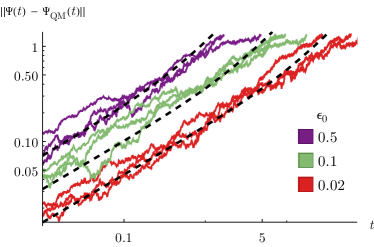
(a) $n=4$

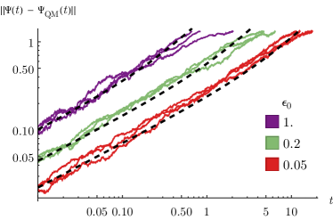
(b) $n=6$

(c) $n=4$

(d) $n=6$

Figure 2: (a-b) To validate our error estimates, we plot the deviation $\varepsilon(t)=||\Psi(t)-\Psi_{\text{QM}}(t)||$ vs time $t$ between the quantum mechanics (QM) wavefunction $\Psi_{\text{QM}}$ and emergent QM (EmQM) wavefunction $\Psi$ [Eq. (51)] for (a) $n=4$ and (b) $n=6$ qubits using three different random initializations (colored lines) for each choice of the control parameter $\epsilon_{0}$ [see Eq. (79)]. As $\epsilon_{0}$ decreases, the EmQM model becomes increasingly more accurate, roughly agreeing with QM out to time $t\sim\epsilon_{0}^{-1}$. Dashed black lines show the estimated deviation $\varepsilon(t)\sim\sqrt{\epsilon_{0}t+3(\epsilon_{0}t)^{2}}$ [Eq. (78)] for the three different values of $\epsilon_{0}$, which match the simulated data remarkably well. (c-d) To demonstrate that the EmQM model is reproducing nontrivial dynamics, we also plot the $0110$ (and $010110$) component of the $n=4$ (and $n=6$) wavefunctions vs time for QM and the EmQM model with $\epsilon_{0}=0.02$ (and $\epsilon_{0}=0.05$), for which $S=800$ (and $S=1280$) [in accordance with Eq. (79)].

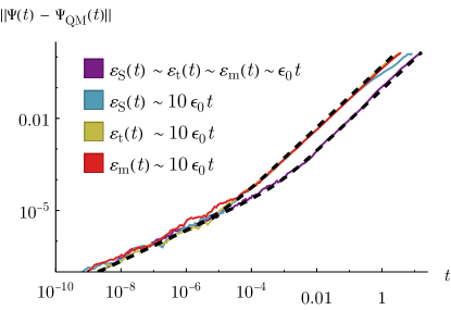
Figure 3: The deviation $\varepsilon(t)=||\Psi(t)-\Psi_{\text{QM}}(t)||$ from quantum mechanics (QM) vs time $t$. The deviation is dominated by statistical fluctuations $\varepsilon_{\text{stat}}(t)$ until the change in slope, after which the deviation is dominated by other contributions. Blue, yellow, and red lines show dominant contributions from $\varepsilon_{\text{S}}(t)$, $\varepsilon_{\text{t}}(t)$, and $\varepsilon_{\text{S}}(m)$, respectively defined in the legend (with $\varepsilon_{\text{stat}}(t)\sim 10^{-2}\sqrt{\epsilon_{0}t}$ and $\varepsilon_{\text{S}}(t)\sim\varepsilon_{\text{t}}(t)\sim\varepsilon_{\text{m}}(t)\sim\epsilon_{0}t$ whenever unspecified). Simulations are for $n=4$ qubits and $\epsilon_{0}=0.05$ with parameters $S$, $\delta_{\text{t}}$, $m_{0}$, and $\Delta_{\text{m}}$ chosen to target the previously-mentioned contributions [using Eqs. (63), (65), and (70)]. The dashed lines plot the expected deviations $\varepsilon(t)$ using Eq. (76), which agree remarkably well with the simulation data (colored lines).

To numerically verify our theoretical results, we simulate the Hamiltonian $H=\sum_{x}H_{x}$ within the EmQM model with

$$H_{x}=Y_{x}X_{x+1}-Y_{x}$$ (81)

which is a simple choice that satisfies the Hamiltonian constraints (4). To do this, we pick a $\epsilon_{0}$ to define the model parameters according to Eq. (79). We then initialize the $m_{s,x}$ matrices using Gaussian random numbers with standard deviation $m_{0}$ and then subtract a constant from each column such that all columns sum to zero. This random initialization implicitly defines a random wavefunction [via (51)]. We then time evolve the circuit for many steps. $\Psi$ is normalized and extracted from $\bm{P}$ using Eq. (51).

However, simulating the EmQM model is extremely expensive for small $\epsilon_{0}$ or many qubits since the CPU time required to simulate out to time $t$ scales as

$$\text{CPU time}\sim Sn\,t/\Delta_{\text{t}}\sim\frac{N}{\delta_{\text{t}}\Delta_{\text{m}}}t\approx\frac{n^{5}N^{3}}{\epsilon_{0}^{8}}\,t$$ (82)

The first relation follows since $t/\Delta_{\text{t}}$ time steps are required on an $S\times n$ lattice. The second relation is obtained by inserting Eq. (50) for $\Delta_{\text{t}}$. The final expression is valid for the $\epsilon_{0}$ parameterization (79). However, we can approximately simulate the EmQM model with high accuracy using the significantly-faster method defined and verified in Appendix D.

We validate our theory for the EmQM model in Fig. 2 by plotting the deviation $\varepsilon(t)$ of the emergent wavefunction $\Psi$ from the quantum mechanics prediction. We find that the deviation is in agreement with the estimated Eq. (78). This verifies that as the control parameter $\epsilon_{0}$ decreases, the EmQM model deviates less from quantum mechanics. All data is generated using the approximate simulation method (Appendix D) except for the $n=4$ data with $\epsilon_{0}=0.5$ (purple in Fig. 2a), for which we could directly simulate the EmQM model.

The deviations from quantum mechanics shown in Fig. 2 are dominated by the statistical deviation $\varepsilon_{\text{stat}}(t)$. To verify the other contributions to the deviation $\varepsilon(t)$, we solve for parameters $S$, $\delta_{\text{t}}$, $m_{0}$, and $\Delta_{\text{m}}$ such that the statistical deviation is much smaller and such that only one of the other contributions is expected to dominate. This allows us to verify each contribution individually in Fig. 3.

VI Experimental Signatures

VI.1 Many Entangled High-Fidelity Qubits

Evidence that an EmQM model really describes nature might be found by measuring deviations from Schrödinger’s equation, such as the $\varepsilon(t)$ [Eq. (52)] studied in the previous section. In Sec. IV, we calculated several contributions to $\varepsilon(t)$. All contributions to $\varepsilon(t)$ can be made extremely small for very long times by taking $S^{-1}$, $\delta_{\text{t}}$, $m_{0}$, and $\Delta_{\text{m}}$ to be very small. $\varepsilon_{\text{S}}(t)\sim t\sqrt{N/S}$ in Eq. (70) is the only deviation that increases polynomially with $N$. This increase with $N$ is significant because $N=2^{n}$ is exponentially large in the number of qubits $n$. Therefore, even if $S\sim 10^{100}$ or $10^{1000}$, only $n\sim 350$ or $3500$ qubits would be needed to obtain a large deviation $\varepsilon_{\text{S}}(t)\sim 1$ after a short time $t\lesssim 1$.

But what should be the value of $n$? If $n$ is taken to be the number of qubits needed to describe just a mesoscopic region of space, e.g. Avogadro’s number $n\sim 10^{23}$, then a large deviation from quantum mechanics due to $\varepsilon_{\text{S}}(t)$ is already predicted for very short times unless $S$ is extremely large $S\gg 2^{10^{23}}$. Indeed, in Sec. IV.4 we found that our model exhibits nonlocal EmQM dynamics unless $Sn\gg 2^{n}$. Therefore, it seems implausible that the particular EmQM model studied in this work accurately describes a possible EmQM for our universe.

However, we speculate that modifications to our model, such as those discussed in Sec. VII.1, could alleviate the $Sn\gg 2^{n}$ requirement for local dynamics of the emergent wavefunction and thus yield a more useful toy model for EmQM. For example, perhaps deviations from quantum mechanics might only be detectable if $Sn\gg 2^{\widetilde{n}}$, where $\widetilde{n}$ is the number of highly entangled qubits that are measured with high fidelity. This hypothesis has not yet been tested experimentally beyond very modest values of $\widetilde{n}$, but might be tested in the future for gradually increasing values of $\widetilde{n}$ by executing deep quantum circuits using quantum computers. Such experiments would significantly constrain the length $S$ of the extra dimension because of the requirement that $S$ be exponential in $\widetilde{n}$. This idea motivated Ref. Slagle (2021), which proposed to test the validity of quantum mechanics using a Loschmidt echo circuit on many qubits.

VI.2 Bell Inequality Tests

Any attempt to describe quantum reality in terms of an underlying local classical model faces the potential obstacle that locally realistic classical models conform to Bell inequalities which are known to be experimentally violated. Yet our model of EmQM agrees with quantum mechanics to high accuracy and so can be expected to pass such tests.

One way to understand why Bell inequality violation cannot easily exclude our model is to note that the speed of information propagation among the underlying classical bits, though finite, is much faster than the emergent speed of light on the boundary. This feature makes it exceedingly hard to close the “locality loophole” — that is, to rule out communication between Alice’s and Bob’s labs during the test.

The classical bits carry information at the speed

$$v_{\text{fast}}\approx\frac{l_{0}}{\Delta_{\text{t}}}\approx\frac{l_{0}}{\Delta_{m}\delta_{\text{t}}}\frac{N}{Sn}$$ (83)

where $l_{0}$ is the spatial distance between bits and where $\Delta_{\text{t}}$ [Eq. (50)] is how much time elapses in the EmQM for each discrete time step. If, for example, we insert the $\epsilon_{0}$ parameterization from Eq. (79) and neglect negligible factors of $n$, we obtain:

$$v_{\text{fast}}\sim\frac{l_{0}}{t_{0}}N^{2}\epsilon_{0}^{-6}$$ (84)

where $t_{0}^{-1}\sim||H_{x}||_{\text{op}}$ is the norm of the local terms in the Hamiltonian (which we previously set to be roughly equal to 1). However, according to local quantum mechanics, all particle velocities (e.g. the speed of light) should be upper bounded by $v_{\text{QM}}\sim l_{0}/t_{0}$. Therefore, since $v_{\text{fast}}\gg v_{\text{QM}}\geq c$, Bell tests cannot easily detect signatures of our model.

VII Outlook

In future work, it will be interesting to investigate how generic emergent quantum mechanics (EmQM) is. That is, if our model is changed slightly, will EmQM still be exhibited? Or do additional ingredients need to be added to our model such that EmQM is a generic result? Or from another point of view, can EmQM be thought of as a highly-exotic phase of classical matter? In a sense, research showing that quantum mechanics is “an island in theory space” Aaronson (2004a) that can be derived axiomatically Hardy (2001); Kapustin (2013); Chiribella et al. (2015) suggests that EmQM might indeed be a stable fixed point under coarse-graining in a broad class of local classical models. It would also be useful to determine if EmQM can result without relying on very small parameters (e.g. $\delta_{\text{t}}$, $m_{0}$, and $\Delta_{\text{m}}$).

VII.1 Mitigating Nonlocality

As emphasized in Sec. VI.1, a crucial remaining future direction is to determine if modifications of our EmQM model could alleviate the $Sn\gg 2^{n}$ requirement for local EmQM dynamics. We would prefer to have an EmQM model such that $S\gg 2^{\widetilde{n}}$ implies consistency with any experiment that only probes $\widetilde{n}$ highly entangled qubits with high fidelity, e.g. the logical qubits in a quantum computer. This would be desirable because only $\widetilde{n}\sim\log_{2}S$ highly entangled qubits would be needed to experimentally test such a model of EmQM, which would be experimentally relevant in the near-term if e.g. $S\sim 2^{1000}$.

Nonlocal dynamics when $Sn\ll 2^{n}$ in our model may result because the stochastic circuits we consider are not very efficient at encoding the wavefunction. In particular, the emergent wavefunction is encoded using random permutation matrices. This inefficient encoding could be contrasted with MERA tensor networks Vidal (2008) or deep neural networks, where each layer can perform a more useful entanglement renormalization Evenbly and Vidal (2015) or coarse graining Mehta and Schwab (2014).

One possible approach to achieve more efficient circuits could be to relax the requirement (25) that the stochastic matrices $M_{s,x}$ are perturbatively close to permutation matrices. But then the subleading (i.e. all but the largest) singular values of $M_{S\leftarrow s}$ [Eq. (56)] will generically be exponentially small in $S-s$. If that occurs, then the overwhelming majority of singular values of $\widetilde{\mathcal{W}}$ [Eq. (58)] will also be extremely small, which will lead to emergent dynamics [Eq. (57)] that do not approximate quantum mechanics well. In this scenario, deep circuits of stochastic matrices are not useful because each layer destroys too much information.

To mitigate this problem, we could consider promoting the classical bits to real numbers. Then the permutation matrices of two bits are promoted to invertible functions from $\mathbb{R}^{2}$ to $\mathbb{R}^{2}$, which can be viewed as a permutation of $\mathbb{R}^{2}$. But unlike permutation matrices, such functions can map the uniform distribution to a different probability distribution. Furthermore, this map can be perfectly inverted. Therefore, unlike deep circuits of generic stochastic matrices, deep circuits of functions do not destroy information. Composing a deep circuit of functions in this way can produce arbitrary probability distributions (and thus arbitrary wavefunctions for EmQM), an observation which has been utilized within the deep learning community Jimenez Rezende and Mohamed (2015); Grathwohl et al. (2018).

VII.2 Quantum Computation and Fundamental Physics

If quantum mechanics does emerge from classical mechanics, then the computational power of quantum computers could be severely limited ’t Hooft (2014); Slagle (2021). For example, BQP-hard problems may only be tractable in actual devices for limited problem sizes. On the other hand, it is possible that deviations from quantum mechanics (such as nonlinear corrections to the Schrödinger equation) could enhance the power of quantum computers Abrams and Lloyd (1998); Aaronson (2004b) for some problems of (possibly) limited size.

Even more speculatively, discovering that quantum mechanics emerges from an underlying local classical model might open new directions for understanding dark matter, dark energy, early-universe cosmology, and the black hole information paradox Carlip (2008). Finally, that our EmQM model encodes the quantum wavefunction on the boundary of an extra spatial dimension suggests possible connections to holographic duality in quantum gravity Hubeny (2015).

Appendix A Measurements

In this appendix, we clarify how measurements could be interpreted in our model within the Everett interpretation of quantum theory. We also speculate how possible improvements upon our EmQM model might lead to a resolution of the measurement problem.

A.1 Everett Interpretation Review

In the Everett interpretation, the observer is included in the wavefunction. In principle, the measurement process can then be formalized as a Hamiltonian evolution via Schrödinger’s equation. After the measurement, Schrödinger’s equation predicts that the observer becomes entangled with the measured system. That is, the resulting wavefunction is in a superposition of states, where each state describes one of the measurement outcomes (from the observer’s perspective).

For example, consider an observer who measures whether the state of a spin is $\ket{\uparrow}$ or $\ket{\downarrow}$. Before the measurement, suppose that wavefunction of the spin is

$$\ket{\psi_{\text{before}}}=a\ket{\uparrow}+b\ket{\downarrow}$$ (85)

In the Everett interpretation, we imagine describing the measurement process using a wavefunction $\ket{\Psi}$ for the entire universe. Before the measurement, we schematically write the universe’s wavefunction as

$$\ket{\Psi_{\text{before}}}=\ket{\mathsf{observer}}\otimes(a\ket{\uparrow}+b\ket{\downarrow})$$ (86)

where $\ket{\mathsf{observer}}$ is the wavefunction for the observer (and the rest of the universe other than the spin). After the measurement (assuming it is performed perfectly), the wavefunction of the universe should be

$$\ket{\Psi_{\text{after}}} =a\ket{\mathsf{observer\ sees}\uparrow}\otimes\ket{\uparrow}$$ (87)

$$+\,b\ket{\mathsf{observer\ sees}\downarrow}\otimes\ket{\downarrow}$$

where $\ket{\mathsf{observer\ sees}\uparrow}\otimes\ket{\uparrow}$ is the wavefunction of the universe where the observer has observed the $\ket{\uparrow}$ state, and similar for $\ket{\mathsf{observer\ sees}\downarrow}\otimes\ket{\downarrow}$.

This exemplifies that in the Everett interpretation, the wavefunction consists of a superposition of all measurement outcomes. The different states in the superposition are macroscopically different and are consequently extremely unlikely to significantly interfere with each other. These different states effectively behave as different “worlds.” Indeed, this interpretation is also often referred to as the many-worlds interpretation.

But then how does one predict the probability that an observer will measure a given outcome (from the observer’s perspective)? Born’s rule implies that the probabilities for the two states, or worlds, in Eq. (87) are $|a|^{2}$ and $|b|^{2}$. But in the Everett interpretation, there are no measurement axioms or applications of Born’s rule; only Schrödinger’s equation is used to evolve the wavefunction. In Schrödinger’s equation, $a$ and $b$ are just coefficients in a linear expansion, and it is not clear why or how these coefficients should be assigned to probabilities associated with the observer’s experience.

Nevertheless, many authors have argued Deutsch (1999); Wallace (2009); Carroll and Sebens (2014); Zurek (2018); Masanes et al. (2019); Hossenfelder (2021); boo (2012) that Born’s rule is the only reasonable or consistent choice, under various reasonable assumptions. For example, Ref. Hossenfelder (2021) gives a brief argument that merely assumes unitary invariance, continuity, and system size invariance. Yet, it remains controversial whether the Everett interpretation (without measurement axioms) provides a complete description of quantum theory Kent (2009).

A.2 EmQM and the Everett Interpretation

In our EmQM model, the slow time dynamics of the boundary degrees of freedom can be accurately predicted using Schrödinger’s equation. That is, there is an emergent wavefunction [$\Psi$ in Eq. (2)] whose time dynamics can be well-approximated by Schrödinger’s equation. Similar to Everett’s interpretation, neither measurement axioms nor Born’s rule explicitly appear in our EmQM model. Thus we are left with a similar challenge as in Everett’s interpretation: does Born’s rule somehow follow from the equations of motion alone?

But for a model of EmQM from classical mechanics, we would not expect the emergent wavefunction to be able to store very many different worlds in superposition. Instead, there must eventually be some sort of “collapse” of the emergent wavefunction to only a subset of the superposed measurement outcomes. Importantly, this collapse of states should be (at least approximately) consistent with Born’s rule if the EmQM model closely approximates standard quantum theory. Perhaps an EmQM model with this property could provide a satisfying solution to the measurement problem.

Unfortunately, our EmQM model does not appear to be successful enough to study this hypothetical wavefunction collapse. As explained in Sec. VI.1, in a certain limit with an extremely large extra dimension, our model simply reproduces Schrödinger’s equation. Therefore this limit is similar to the Everett interpretation, and it is not obvious how the measurement probabilities for an observer should be assigned, although some of the arguments in Refs. Deutsch (1999); Wallace (2009); Carroll and Sebens (2014); Zurek (2018); Masanes et al. (2019); Hossenfelder (2021); boo (2012) might still be applicable. If the extra dimension isn’t sufficiently large, then there are nonlocal violations of Schrödinger’s equation, but we have no reason to expect these violations to imply an approximate version of Born’s rule (although we have not checked thoroughly). It seems that better models are needed to assess whether the Born rule, in addition to Schrödinger’s equation, could arise from a sensible classical model of EmQM.

Appendix B Real-valued Quantum Mechanics

In this appendix, we show that any quantum Hamiltonian and wavefunction in Schrödinger’s equation can be linearly mapped to real-valued analogs with zero row and column sums that satisfy Eqs. (3–4) while preserving locality. We do this by first mapping to real-valued quantum mechanics McKague et al. (2009); Aleksandrova et al. (2013); Stueckelberg (1960); Myrheim (1999) in Appendix B.1 and then focus on zero sums in Appendix B.2.

Both mappings generically require adding additional qubits. Preserving locality requires multiplying the qubit count by a constant factor (when using the systematic mapping). As a result, the possible real-valued wavefunctions that result from this mapping are highly constrained in the sense that these wavefunctions only span a subset of the Hilbert space. Therefore, although there are well-known fundamental differences between complex and real-valued quantum mechanics Aaronson (2004a); Renou et al. (2021); Li et al. (2022); Chen et al. (2022); Hardy (2001); Caves et al. (2000, 2002), this mapping shows that complex-valued quantum mechanics is equivalent to real-valued quantum mechanics constrained to a subspace of the Hilbert space. However in Appendix B.1.3, we emphasize that in real-valued quantum mechanics, it is not correct to assume that “the state representing two independent preparations of the two systems is the tensor product of the two preparations” Renou et al. (2021).

B.1 Mapping from Complex to Real QM

B.1.1 Geometrically nonlocal Mapping

If we do not require that the mapping is geometrically local, then mapping to real values can be achieved simply by splitting complex numbers into their real and imaginary parts McKague et al. (2009); Aleksandrova et al. (2013); Stueckelberg (1960). This can be achieved for operators via the replacement

$$i\to-i\sigma^{2}$$ (88)

where

$$\sigma^{2}=\begin{pmatrix}0&-i\\ i&0\end{pmatrix}$$ (89)

is a Pauli operator acting on an additional qubit.

We note that

$$\ket{\pm i}=\tfrac{1}{\sqrt{2}}\big{(}\ket{\uparrow}\pm i\ket{\downarrow}\big{)}.$$ (90)

are eigenstates of $\sigma^{2}$ with eigenvalues $\pm 1$, and that

$$P(\pm)=\tfrac{1}{2}\left(\mathbbl{1}\pm\sigma^{2}\right)$$ (91)

are orthogonal projectors onto these eigenstates. Furthermore, $\ket{+i}$ and $\ket{-i}$ are complex conjugates of one another, as are $P(+)$ and $P(-)$. We map an $n$-qubit wavefunction $\ket{\psi}$ to a real $(n{+}1)$-qubit wavefunction $\ket{\widetilde{\psi}}$ according to

$$\ket{\psi}\to\ket{\widetilde{\psi}}=\tfrac{1}{\sqrt{2}}\big{(}\ket{\psi}\otimes\ket{-i}+\ket{\psi}^{*}\otimes\ket{+i}\big{)},$$ (92)

and map an $n$-qubit operator $Q$ to a real $(n{+}1)$-qubit operator $\widetilde{Q}$ according to

$$Q\to\widetilde{Q}=Q\otimes P(-)+Q^{*}\otimes P(+)$$ (93)

where * denotes complex conjugation; thus

$$\widetilde{Q}\ket{\widetilde{\psi}}=\tfrac{1}{\sqrt{2}}\big{(}Q\ket{\psi}\otimes\ket{-i}+Q^{*}\ket{\psi}^{*}\otimes\ket{+i}\big{)}.$$ (94)

Under this mapping, Schrödinger’s equation $\partial_{t}\ket{\psi(t)}=-iH\ket{\psi(t)}$ is equivalent to

$$\partial_{t}\ket{\widetilde{\psi}(t)}=-(\widetilde{iH})\ket{\widetilde{\psi}(t)}.$$ (95)

That is, it is mapped to Schrödinger’s equation for the real wavefunction $\ket{\widetilde{\psi}}$ with imaginary Hamiltonian $-i(\widetilde{iH})$, where $\widetilde{iH}$ denotes the result of mapping $Q=iH$ using Eq. (93).

Another way to express the mapping is sometimes convenient. Note that if $Q$ is real, then

$$\widetilde{Q}=Q\otimes\mathbbl{1},$$ (96)

while if $Q$ is imaginary, then

$$\widetilde{Q}=(-iQ)\otimes(-i\sigma^{2});$$ (97)

more generally

$$\widetilde{Q}=\operatorname{Re}Q\otimes\mathbbl{1}+\operatorname{Im}Q\otimes(-i\sigma^{2}).$$ (98)

Similarly, if $\ket{\psi}$ is real in some basis, then

$$\ket{\widetilde{\psi}}=\ket{\psi}\otimes\ket{\uparrow},$$ (99)

while if $\ket{\psi}$ is imaginary, then

$$\ket{\widetilde{\psi}}=-i\ket{\psi}\otimes\ket{\downarrow};$$ (100)

and more generally

$$\ket{\widetilde{\psi}}=\ket{\operatorname{Re}\psi}\otimes\ket{\uparrow}+\ket{\operatorname{Im}\psi}\otimes\ket{\downarrow}.$$ (101)

B.1.2 Local Mapping

Now suppose that $H=\sum_{x}H_{x}$ is a local Hamiltonian, where each $H_{x}$ only acts on qubits near the spatial point $x$. If $H_{x}$ and $H_{y}$ act on sets of qubits that are distantly separated from one another, then it’s not possible to put the additional qubit close to both sets. Therefore, the above operator map does not preserve the geometric locality of the Hamiltonian.

In order to promote the nonlocal mapping to a mapping that preserves locality for local operators $Q_{x}$, we can instead add a new qubit adjacent to each lattice site and map

$$i\to-i\sigma_{x}^{2}$$ (102)

at each site. Wavefunctions are then mapped according to

$$\ket{\psi} \to\ket{\widetilde{\psi}}=\tfrac{1}{\sqrt{2}}\big{(}\ket{\psi}\operatorname*{\text{\scalebox{1.2}{$\otimes$}}}_{x}\ket{-i}_{x}+\ket{\psi}^{*}\operatorname*{\text{\scalebox{1.2}{$\otimes$}}}_{x}\ket{+i}_{x}\big{)}.$$ (103)

Now suppose that $Q_{x}$ is a $k$-local operator (e.g. a term in the Hamiltonian) acting on $k$ qubits near $x$. After the mapping, the site $x$ is accompanied by an adjacent auxiliary qubit, and $Q_{x}$ is mapped to

$$\widetilde{Q}_{x}=Q_{x}\otimes P(-)_{x}+Q_{x}^{*}\otimes P(+)_{x},$$ (104)

a $(k+1)$-local operator acting on the $k$ qubits together with the auxiliary qubit adjacent to site $x$. Another way to express the mapping is

$$\widetilde{Q}_{x}=\operatorname{Re}Q_{x}\otimes\mathbbl{1}_{x}+\operatorname{Im}Q_{x}\otimes(-i\sigma_{x}^{2}).$$ (105)

Thus the $k$-local Hamiltonian $H=\sum_{x}H_{x}$ can be mapped to the $(k+1)$-local Hamiltonian $\widetilde{H}=\sum_{x}\widetilde{H_{x}}$.

As we found for the nonlocal mapping, Schrödinger’s equation $\partial_{t}\ket{\psi(t)}=-iH\ket{\psi(t)}$ is equivalent to to Schrödinger’s equation for the real wavefunction $\ket{\widetilde{\psi}}$ with imaginary Hamiltonian

$$-i(\widetilde{iH})=\sum_{x}\left(i\operatorname{Im}(H_{x})\otimes\mathbbl{1}_{x}-\operatorname{Re}(H_{x})\otimes\sigma_{x}^{2}\right).$$ (106)

B.1.3 Dynamics

Here we briefly review some dynamical properties of real-valued quantum mechanics. We want $iH$ to be real such that no imaginary values appear in Schrödinger’s equation, which implies that $H$ must be imaginary and antisymmetric. Thus for each eigenvector $\ket{E}$, taking the complex-conjugate of $H\ket{E}=E\ket{E}$ (in any basis) implies that the complex-conjugated $\ket{E}^{*}$ has eigenvalue $-E$. Therefore, eigenvectors with nonzero eigenvalues come in complex-conjugate pairs with negated eigenvalues. It is convenient to consider real-valued linear combinations $\ket{E}_{\pm}=\tfrac{1}{\sqrt{\pm 2}}(\ket{E}\pm\ket{-E})$ for each $E>0$. The coefficients $a_{E,\pm}(t)$ of a wavefunction $\ket{\psi(t)}=\sum_{E,\pm}a_{E,\pm}(t)\ket{E}_{\pm}$ obey the time evolution $\partial_{t}a_{E,\pm}(t)=\mp Ea_{E,\mp}(t)$ for each $E>0$.

A real-valued wavefunction can not be in an eigenstate $\ket{E}$ with nonzero $E$ since $\ket{E}$ is complex-valued when $E\neq 0$. In complex-valued quantum mechanics, eigenstates are steady-states, i.e. states that do not change with time. The analog of steady-states in real-valued quantum mechanics are oscillating superpositions of $\ket{E}_{\pm}$:

$$\ket{\psi(t)} =\cos(Et)\ket{E}_{+}-\sin(Et)\ket{E}_{-}$$ (107)

$$=\tfrac{1}{\sqrt{2}}e^{-iEt}\ket{E}+\tfrac{1}{\sqrt{2}}e^{+iEt}\ket{-E}.$$

The analog of the lowest-energy ground state is the above state with the largest possible $E$. Notably, this “steady-state” looks like a cat state from the perspective of complex-valued quantum mechanics. Indeed, the steady-state of two disconnected subsystems will share an entangled qubit from the perspective of complex-valued quantum mechanics. For example, if $H=-Y_{1}-Y_{2}$ is the Hamiltonian for two qubits, then the lowest-energy steady-state is not a tensor product state; instead, it is maximally entangled:

$$\ket{\psi(t)} =\big{(}\cos(t)\ket{\uparrow}-\sin(t)\ket{\downarrow}\big{)}\otimes\big{(}\cos(t)\ket{\uparrow}-\sin(t)\ket{\downarrow}\big{)}$$ (108)

$$\,-\big{(}\sin(t)\ket{\uparrow}+\cos(t)\ket{\downarrow}\big{)}\otimes\big{(}\sin(t)\ket{\uparrow}+\cos(t)\ket{\downarrow}\big{)}.$$

In complex-valued quantum mechanics, the following tensor product axiom holds for combining quantum states of two systems: “the state representing two independent preparations of the two systems is the tensor product of the two preparations” Renou et al. (2021). However, this axiom does not hold in real-valued quantum mechanics. Indeed, Ref. Chen et al. (2022); Li et al. (2022) have verified that real-valued quantum mechanics with this tensor product axiom is not consistent with experiment. Nevertheless, our analysis above shows that real-valued quantum mechanics is consistent with complex-valued quantum mechanics if the tensor product axiom is dropped. Indeed the tensor product axiom is not consistent with our local mapping (103), which maps complex-valued tensor product wavefunctions to a sum of two tensor products. Furthermore, Eq. (108) shows that a sum of two tensor products arises naturally for ground state wavefunctions of two disconnected subsystems in real-valued quantum mechanics.

B.2 Zero Sum

To satisfy the zero-sum conditions (3–4), we once again introduce an additional qubit. We map the wavefunction $\ket{\psi}$ to

$$\ket{\widetilde{\psi}}=\ket{\psi}\otimes\ket{-}$$ (109)

where

$$|-\rangle=\tfrac{1}{\sqrt{2}}\big{(}\ket{\uparrow}-\ket{\downarrow}\big{)}.$$ (110)

Similarly, any operator $Q$ can be linearly mapped to a new operator

$$\widetilde{Q}=Q\otimes|-\rangle\langle-|,$$ (111)

where

$$|-\rangle\langle-|=\tfrac{1}{2}\big{(}\ket{\uparrow}\bra{\uparrow}-\ket{\uparrow}\bra{\downarrow}-\ket{\downarrow}\bra{\uparrow}+\ket{\downarrow}\bra{\downarrow}\big{)}.$$ (112)

By construction, $\ket{\widetilde{\psi}}$ and $\widetilde{Q}$ obey the zero-sum conditions:

$$\sum_{i}\widetilde{\psi}_{i} =0$$ (113)

$$\sum_{i}\widetilde{Q}_{ij} =0=\sum_{j}\widetilde{Q}_{ij}.$$

in any basis where the additional qubit has basis vectors $\ket{\uparrow}$ and $\ket{\downarrow}$. Furthermore, the zero-sum constraints are preserved under evolution under the Schrödinger equation for a Hamiltonian that obeys the zero-sum constraints.

In order to preserve geometric locality, we add another set of new qubits adjacent to each $x$. The mapping for wavefunctions and local operators (including terms in the Hamiltonian) is

$$\ket{\psi} \to\ket{\widetilde{\psi}}=\ket{\psi}\otimes_{x}\ket{-}_{x}$$ (114)

$$Q_{x} \to\widetilde{Q}_{x}=Q_{x}\otimes\ket{-}_{x}\bra{-}_{x}.$$ (115)

B.3 Examples

B.3.1 Ising (systematic mapping)

As an example, we can consider applying these systematic mappings to a transverse-field Ising model Hamiltonian $H=\sum_{x}H_{x}$:

$$H_{x} =-JZ_{x}Z_{x+1}-hY_{x}$$

$$\to JZ_{x}Z_{x+1}\otimes\sigma^{2}_{x}-hY_{x}$$ (116)

$$\to\left(JZ_{x}Z_{x+1}\otimes\sigma^{2}_{x}-hY_{x}\right)\otimes\ket{-}_{x}\bra{-}_{x}.$$

$X_{x}$, $Y_{x}$, $Z_{x}$ are Pauli operators in the Ising model Hamiltonian, while $\sigma_{x}^{2}$ is a Pauli operator acting on additional qubits. $\ket{-}_{x}\bra{-}_{x}$ acts on an additional set of qubits. A transverse $hY_{x}$ term was considered in the first line instead of the traditional $hX_{x}$ term to make the example more useful. The second line is the result of applying Eq. (106) to obtain an imaginary-valued Hamiltonian. Eq. (115) is applied to obtain the third line, for which the resulting Hamiltonian has zero row and column sums.

B.3.2 Ising (clever duality)

However, adding additional qubits is not always necessary. For example, the XY Hamiltonian is dual to an imaginary-valued Hamiltonian with zero row and column sums:

$$H_{x} =-J_{XY}\,(X_{x}X_{x+1}+Y_{x}Y_{x+1})$$ (117)

$$\leftrightarrow J_{\text{XY}}\,(X_{x-1}Y_{x}X_{x+1}-Y_{x})$$ (118)

The second Hamiltonian describes the phase transition between a SPT cluster state Son et al. (2012) and the trivial disorered phase.

The duality mapping used above is:

$$Y_{x}Y_{x+1} \leftrightarrow Y_{x}$$ (119)

$$Z_{x} \leftrightarrow X_{x-1}X_{x}$$

which implies that $X_{x}X_{x+1}\leftrightarrow-X_{x-1}Y_{x}X_{x+1}$. This duality only maps symmetric operators to local operators. Symmetric operators are operators that commute with certain $Z_{2}$ symmetries, which are $\prod_{x}Z_{x}$ and $\prod_{x}Y_{x}$ for the respective left and right sides of the duality. The duality maps the $Z_{2}$ symmetries to the identity (ignoring boundary conditions):

$$\prod_{x}Z_{x} \leftrightarrow 1$$ (120)

$$1 \leftrightarrow\prod_{x}Y_{x}$$

These properties are common in duality mappings, such as the self-duality Radicevic (2018) of the transverse-field Ising model.

Appendix C Emergent Lorentz Invariance

In Sec. II.1, we had to posit that the observed Lorentz invariance in our universe is emergent (rather than exact). This may not be a major hurdle since emergent Lorentz invariance has been shown to be a stable fixed point under the renormalization group (RG) in several strongly-coupled models Roy et al. (2016); Bednik et al. (2013); Belenchia et al. (2016). Indeed, emergent Lorentz invariance is rather ubiquitous in low-energy physics. For example, emergent Lorentz invariance occurs in materials such as graphene, which exhibits an electron band structure with a Lorentz-invariant Dirac cone at low energy. As a result, the electrons in graphene experience a Lorentz-invariant speed limit that is much smaller than the speed of photons.

But with multiple species of fermions, emergent Lorentz invariance would require that all Dirac fermions have the same velocity. Although the velocities for different species flow to the same value under RG, the flow is very slow; hence emergent Lorentz invariance seems to require fine tuning in order to be consistent with certain very precise experiments. Collins et al. (2004); Polchinski (2012) Furthermore, general relativity would likely also need to be emergent in this scenario Laughlin (2003); Carlip (2012).

It is not clear if including the effects of a fully quantized theory of emergent quantum gravity could significantly affect the RG flow such that Lorentz invariance emerges more rapidly. In particular, we note that when Lorentz invariance is broken, the local diffeomorphism “gauge symmetry” of general relativity is broken. This reminds us of $(3+1)$-dimensional U(1) gauge theory, in which we could imagine adding an $A^{2}=A_{\mu}A^{\mu}$ term to the Lagrangian, which breaks the gauge symmetry. However, although $A^{2}$ naively appears to be relevant in $(3+1)$ dimensions since $A^{2}$ has energy dimension 2, $A^{2}$ is actually an irrelevant perturbation. In fact, all perturbations to $(3+1)$-dimensional U(1) gauge theory are irrelevant, including the perturbations that break gauge invariance Hermele et al. (2004).

We emphasize that although these gauge-symmetry-breaking terms are irrelevant for the compact gauge group U(1), such terms are relevant (as naively expected) for the non-compact gauge group $\mathbb{R}$. Note that both of these gauge groups lead to the same classical equations of motion since they have the same Lie algebra. It is remarkable that it is only after quantizing these two different gauge theories, with gauge groups U(1) or $\mathbb{R}$, that we discover that gauge invariance can be emergent in U(1) gauge theory but not in $\mathbb{R}$. With this in mind, we speculate that emergent Lorentz invariance may occur sufficiently rapidly in some theories of emergent gravity such that it could be consistent with experiments. Gu and Wen (2006)

One approach to intuitively understanding why $A^{2}$ is irrelevant in U(1) gauge theory is to consider the corresponding lattice gauge theory (without constraining the Hilbert space to the gauge-invariant states). The lattice gauge theory is similar to the toric code Kitaev (2003), except the $Z_{2}$ qubits are replaced by integer-valued degrees of freedom $E_{e}\in\mathbb{Z}$ on each edge $e$ of the lattice. The Hamiltonian is $H=\sum_{i}(\nabla_{i}n)^{2}-\sum_{p}\cos(\nabla_{p}\times A)$. $\nabla_{i}n$ denotes the lattice divergence of $n_{e}$ centered at the vertex $i$, while $\nabla_{p}\times A$ is the lattice curl of $A_{e}$ around the plaquette $p$. The commutation relations are $[e^{iA_{e}},n_{e^{\prime}}]=\delta_{e,e^{\prime}}$. The states with $\nabla_{i}n=0$ obey Gauss’s law and are the gauge-invariant states.

Gauge invariance is often imposed by taking $\nabla_{i}n=0$ to be a constraint on the Hilbert space. Here, we do not constrain the Hilbert space; instead we use the first term of the Hamiltonian to impose an energy penalty on states that are not gauge invariant. Since $n_{e}$ is integer valued, all energy excitations of $\sum_{i}(\nabla_{i}n)^{2}$ cost finite energy, which makes the gauge invariance stable to perturbations. For example, a $\epsilon A^{2}$ term in the U(1) gauge theory Lagrangian is analogous to a $\epsilon\sum_{e}\cos(A_{e})$ term in the lattice gauge theory Hamiltonian. If $\epsilon$ is sufficiently small, this term does not does not lead to confinement since its excitations cost finite energy due to the $(\nabla_{i}n)^{2}$ term. This can be shown more formally using degenerate perturbation theory Bravyi et al. (2011). Similarly, in the toric code (i.e. $Z_{2}$ lattice gauge theory where Gauss’s law enters the Hamiltonian as an energy penalty rather than a Hilbert space constraint), arbitrary perturbations are irrelevant and do not destabilize the emergent gauge invariance or topological order. Kitaev (2003)

We emphasize that even if there are faster-than-light degrees of freedom, it could still be very difficult for observers to send information faster than light. Suppose a Hamiltonian $H$ is Lorentz-invariant (either exactly or approximately at low energies) with velocity $c$, and suppose an observer living within the wavefunction $\Psi$ wants to use the fast classical degrees of freedom to send signals faster than $c$ (without exceeding low energies if the Lorentz-invariance is approximate). If $\Psi(t)$ is well-described by Schrödinger’s equation for a local Hamiltonian, then the observer will only be able to send signals much faster than $c$ by taking advantage of very small possible violations of Schrödinger’s equation Polchinski (1991); Gisin (1990).

Appendix D Approximate Simulation

As noted in Eq. (82), simulating the EmQM model is very CPU intensive. Fortunately, we can approximately simulate the EmQM model significantly faster by “integrating out” the fast degrees of freedom (i.e. the forward and backward-propagating bits) so that we only have to directly simulate the slow degrees of freedom (i.e. the stochastic matrices). This will allow us to simulate $\Delta_{\text{jump}}\gg S$ many time steps all at once with negligible error.

To do this, we approximate the stochastic matrices $M_{s,x}$ as constant over $\Delta_{\text{jump}}$ many time steps. We then estimate how much the stochastic matrices might change after these $\Delta_{\text{jump}}$ time steps. If $\Delta_{\text{jump}}\gg N=2^{n}$, then each bit string will occur many times over this many time steps. Therefore, simulating the propagation of $\Delta_{\text{jump}}$ many bit strings involves a lot of duplication of effort. To speed up the simulations, we can instead just calculate how much each stochastic matrix will be affected by the propagation of all $N$ possible bit strings, each weighted by its probability times $\Delta_{\text{jump}}$.

D.1 Approximate Algorithm

The approximate algorithm to compute how $\Delta_{\text{jump}}$ time steps could affect the stochastic matrices is as follows:

We first compute $\bm{P}_{S}^{(\tau)}$ using Eq. (23) to get the probability vector for the output bits $a_{S}$ of the stochastic circuit.

Then for each $\gamma=1,2$, we sample an $N\times N$ matrix $\beta_{S,\gamma}^{(\tau)}$ from the multinomial distribution of $\Delta_{\text{jump}}$ trials with a matrix of probabilities $(B^{(+\gamma)}\cdot\bm{P}_{S}^{(\tau)})\otimes(B^{(-\gamma)}\cdot\bm{P}_{S}^{(\tau)})$, where $B^{(\gamma)}$ is the $N\times N$ stochastic matrix defined in Eq. (18). Therefore, $\beta_{S,\gamma}^{(\tau)}(b_{S,+\gamma},b_{S,-\gamma})$ counts how many times the pair $(b_{S,+\gamma},b_{S,-\gamma})$ of bit strings could have occurred after $\Delta_{\text{jump}}$ time steps. Note that we approximated $M_{s,x}^{(\tau)}$ as constant over these $\Delta_{\text{jump}}$ time steps.

Next we back-propagate [analogous to Eq. (30)] $\beta_{s,\gamma}^{(\tau)}$ using the permutation matrices $Q_{s}$ defined in Eq. (26):

$$\beta_{s,\gamma}^{(\tau)}=Q_{s}^{T}\cdot\beta_{s+1,\gamma}^{(\tau)}\cdot Q_{s}$$ (121)

Finally, we wish to update the perturbations $m_{s,x}$ in accordance with Eq. (31) using $\beta_{S,\gamma}^{(\tau)}$. To do this, we modify Eq. (31) to

$$m_{s,x}^{(\tau+\Delta_{\text{jump}})}=m_{s,x}^{(\tau)}+\Delta_{\text{m}}\sum_{b{x}^{+}}\sum_{b{x}^{-}}\sum_{e{x}}\Bigg{[}$$ (122)

$$\quad\quad\sum_{\gamma=1,2}\beta_{s,x,\gamma}^{(\tau)}(b{x}^{+},b{x}^{-})\,p_{s,x}^{(\tau)}(e{x}|b{x}^{-})\left(\bm{\hat{b}}{x}^{+}-\bm{\hat{b}}{x}^{-}\right)\otimes\bm{\hat{e}}{x}\Bigg{]}$$

where $b{x}^{+}$, $b{x}^{-}$, and $e{x}$ are each a pair of bits (00, 01, 10, or 11). These bit pairs index the $4\times 4$ matrices $m_{s,x}^{(\tau)}$ and $\beta_{s,x,\gamma}^{(\tau)}$. The bit pairs also determine the basis 4-vectors $\bm{\hat{b}}{x}^{\pm}$ and $\bm{\hat{e}}{x}$; e.g. $\bm{\hat{b}}{x}^{+}=(1,0,0,0)$ if $b{x}^{+}=00$. Above, $\beta_{s,x,\gamma}^{(\tau)}(b{x}^{+},b{x}^{-})$ counts how many times the pair $(b{x}^{+},b{x}^{-})$ could have occurred over the $\Delta_{\text{jump}}$ time steps. That is,

$$\beta_{s,x,\gamma}^{(\tau)}=\sum_{b^{+}}\sum_{b^{-}}\bm{\hat{b}}{x}^{+}\otimes\bm{\hat{b}}{x}^{-}\,\beta_{s,\gamma}^{(\tau)}(b^{+},b^{-})$$ (123)

where $\sum_{b^{\pm}}$ sums over the $N=2^{n}$ different bit strings of $n$ bits, and $\bm{\hat{b}}{x}^{\pm}$ is the basis 4-vector that depends on bits $x$ and $x+1$ of the bit string $b^{\pm}$; e.g. $\bm{\hat{b}}{x}^{\pm}=(1,0,0,0)$ [or $(0,1,0,0)$] if bits $x$ and $x+1$ of $b^{\pm}$ are $00$ [or $01$]. In Eq. (122), $p_{s,x}^{(\tau)}(e{x}|b{x}^{-})$ is a conditional probability distribution for $e{x}$ given $b{x}^{-}$.

We need to calculate $p_{s,x}^{(\tau)}(e{x}|b{x}^{-})$ such that it is approximately equal to the probability that $\bm{\hat{e}}_{s-1,x,\gamma}^{(\tau)}=\bm{\hat{e}}{x}$ given $\bm{\hat{b}}_{s,\mathbbl{x},-\gamma}^{(\tau)}=\bm{\hat{b}}{x}^{-}$ in Eq. (31) over the $\Delta_{\text{jump}}$ time steps. Recall that $\bm{\hat{e}}_{s-1,x,\gamma}^{(\tau)}$ is chosen uniformly at random from the set of basis 4-vectors that keep $M_{s,x}^{(\tau)}=Q_{s,x}+m_{s,x}^{(\tau)}$ non-negative. Therefore we can take $p_{s,x}^{(\tau)}(e{x}|b{x}^{-})=1/4$ to be uniform probabilities as long as this results in a stochastic matrix $M_{s,x}^{(\tau+\Delta_{\text{jump}})}$ with non-negative entries.

However if $M_{s,x}^{(\tau+\Delta_{\text{jump}})}$ has negative entries, then $p_{s,x}^{(\tau)}$ can not be uniform. Instead, for each negative $M_{s,x}^{(\tau+\Delta_{\text{jump}})}(b{x}^{-},e{x})<0$ entry that we find, we must make $p_{s,x}^{(\tau)}(e{x}|b{x}^{-})$ a free parameter [while uniformly adjusting the other entries such that $p_{s,x}^{(\tau)}(e{x}|b{x}^{-})$ is a probability distribution for $e{x}$ given $b{x}^{-}$]. We then solve for these free parameters such that the previously-negative entries of $M_{s,x}^{(\tau+\Delta_{\text{jump}})}$ are zero. If $M_{s,x}^{(\tau+\Delta_{\text{jump}})}$ for the new $p_{s,x}^{(\tau)}$ has additional negative entries, then we repeat the procedure until all entries are non-negative. That is, we make more entries in $p_{s,x}^{(\tau)}$ free parameters and re-solve for the old and new free parameters such that any previously-negative entry of $M_{s,x}^{(\tau+\Delta_{\text{jump}})}$ is zero. At most, $p_{s,x}^{(\tau)}$ can only have $4\times 3$ free parameters, since it describes 4 different probability distributions, each with up to 3 free parameters. Therefore, the above procedure can not repeat more than 12 times. As desired, this procedure results in a $p_{s,x}^{(\tau)}$ that is approximately equal to the probability that $\bm{\hat{e}}_{s-1,x,\gamma}^{(\tau)}=\bm{\hat{e}}{x}$ given $\bm{\hat{b}}_{s,\mathbbl{x},-\gamma}^{(\tau)}=\bm{\hat{b}}{x}^{-}$ in Eq. (31) over the $\Delta_{\text{jump}}$ time steps.

D.2 Approximation Error

The approximate algorithm makes the approximation that $M_{s,x}^{(\tau)}$ is constant over $\Delta_{\text{jump}}$ many time steps. This approximation is very similar to the cause of the deviation $\varepsilon_{\text{delay}}(t)$ [Eq. (75)] that results from the $O(S)$ discrete time delay for the classical bits to move through the circuit. The primary difference is that the delay is $\Delta_{\text{jump}}$ instead of $O(S)$ for the approximate algorithm. Therefore, the approximate algorithm results in an error similar to Eq. (75), except a factor of $S$ is replaced by $\Delta_{\text{jump}}$:

$$\varepsilon_{\text{jump}}(t) \sim\frac{\Delta_{\text{jump}}}{S}\varepsilon_{\text{delay}}(t)$$ (124)

$$\sim n\Delta_{t}\Delta_{\text{jump}}\,t$$

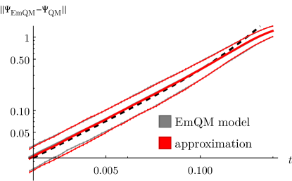
Figure 4: The deviation $||\Psi(t)-\Psi_{\text{QM}}(t)||$ vs time $t$ for $n=4$ qubits with $\epsilon_{0}=1$, showing agreement between the EmQM model (gray), approximate algorithm with $\epsilon_{\text{j}}=0.02$ (red), and estimated $\varepsilon(t)$ from Eq. (78) (dashed black). For the EmQM model and approximate algorithm, we average over 1000 random realizations and plot the mean (thick lines) along with the mean plus/minus the standard deviation (thin lines) to demonstrate that both the mean and statistical fluctuations agree well. Error bars denote one standard deviation of statistical error resulting from the finite number of 1000 samples.

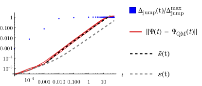
Figure 5: The deviation $||\Psi(t)-\Psi_{\text{QM}}(t)||$ (red) vs time $t$ calculated using the approximate algorithm with a large $\varepsilon_{\text{jump}}=10$ so that we can study errors due to the approximate simulation algorithm. Simulations use $n=4$ qubits and three different random initializations with $\varepsilon=0.01$ [in Eq. (79)]. In all simulations in this work, $\Delta_{\text{jump}}$ is chosen to be as large as possible without exceeding $\Delta_{\text{jump}}^{\text{max}}$. $\Delta_{\text{jump}}$ is sometimes limited (shown by blue dots) when the time step is very small (due to the logarithmic time axis). By inserting the actual time-dependent $\Delta_{\text{jump}}(t)$ into Eq. (124), our estimate $\widetilde{\varepsilon}(t)$ [(127), dashed black line] for the deviation (under the influence of the approximation) matches the $\varepsilon_{\text{jump}}(t)$-dominated simulation data (red) remarkably well. In contrast, the dashed gray curve shows the expected deviation $\varepsilon(t)$ of the EmQM model without approximation, which is significantly smaller when $0.01\lesssim t\lesssim 10$. This validates Eq. (127).

In our simulations, we want to choose $\Delta_{\text{jump}}$ to be as large as possible without introducing noticeable errors in our plots. To achieve this, we choose $\Delta_{\text{jump}}$ such that $\varepsilon_{\text{jump}}(t)$ in Eq. (124) is parameterized by a new control parameter $\epsilon_{\text{j}}$:

$$\varepsilon_{\text{jump}}(t)\sim\epsilon_{0}\,\epsilon_{\text{j}}\,t$$ (125)

Small $\epsilon_{\text{j}}$ will then ensure that $\varepsilon_{\text{jump}}(t)$ contributes negligibly to $\varepsilon(t)=||\Psi-\Psi_{\text{QM}}||$ in comparison to the estimated $\varepsilon(t)\sim\sqrt{\epsilon_{0}t}$ in Eq. (78). Therefore, Eq. (124) implies that we must limit $\Delta_{\text{jump}}$ to be no larger than

$$\Delta^{\text{max}}_{\text{jump}} \approx\frac{\epsilon_{0}\,\epsilon_{\text{j}}}{\Delta_{t}n}$$ (126)

$$\sim\frac{n^{3}N^{2}}{\epsilon_{0}^{5}}\epsilon_{\text{j}}.$$

Due to this additional source of error, the approximate algorithm will produce slightly larger deviations from quantum mechanics, which we estimate to be

$$\widetilde{\varepsilon}(t)\sim\sqrt{\varepsilon(t)^{2}+\varepsilon_{\text{jump}}(t)^{2}}.$$ (127)

To ensure that the error $\varepsilon_{\text{jump}}(t)$ from the approximate algorithm remains negligible, we use small $\epsilon_{\text{j}}=0.02$ for most simulations (excluding Fig. 5). The only exception is the $\epsilon_{0}=0.05$ data in Fig. 2(b,d), which used $\epsilon_{\text{j}}=0.1$ in order to keep the simulation time under one month.

To validate that our approximate algorithm does not significantly affect the deviation $||\Psi-\Psi_{\text{QM}}||$ or its statistical fluctuations when $\varepsilon_{\text{jump}}$ is small, in Fig. 4 we compare these quantities for the EmQM model and the approximate algorithm. To validate Eq. (127), in Fig. 5 we plot the deviation $||\Psi(t)-\Psi_{\text{QM}}(t)||$ from quantum mechanics using the approximate model with large $\epsilon_{\text{j}}$ such that the error from approximation dominates.