Properties of the Lowest Metallicity Galaxies Over the Redshift Range $z=0.2$ to $z=1$

Abstract

Low-metallicity galaxies may provide key insights into the evolutionary history of galaxies. Galaxies with strong emission lines and high equivalent widths (rest-frame EW(H$\beta)\gtrsim 30$ Å) are ideal candidates for the lowest metallicity galaxies to $z\sim 1$. Using a Keck/DEIMOS spectral database of about 18,000 galaxies between $z=0.2$ and $z=1$, we search for such extreme emission-line galaxies with the goal of determining their metallicities. Using the robust direct $T_{e}$ method, we identify 8 new extremely metal-poor galaxies (XMPGs) with $12+\log$ O/H $\leq$ $7.65$, including one at $6.949\pm 0.091$, making it the lowest metallicity galaxy reported to date at these redshifts. We also improve upon the metallicities for two other XMPGs from previous work. We investigate the evolution of H$\beta$ using both instantaneous and continuous starburst models, finding that XMPGs are best characterized by continuous starburst models. Finally, we study the dependence on age of the build-up of metals and the emission-line strength.

1 Introduction

Low-redshift ($z\lesssim 1$), low-metallicity galaxies could be the best analogs of small, star-forming galaxies (SFGs) at high redshifts ($z\gtrsim 6$). Such low-redshift galaxies may give insights into the properties of early SFGs, which may be responsible for reionizing the universe. Izotov et al. (2021) found that the properties of low-metallicity, compact SFGs with high equivalent widths (EWs) of the H$\beta$ emission line are similar to the properties of high-redshift SFGs.

The lowest metallicity galaxies are often called extremely metal-poor galaxies (XMPGs). These are defined as galaxies with metallicities $12+\log$ O/H $\leq$ $7.65$, which is $1/10$th of the solar metallicity (8.65; Asplund et al., 2006). A few dozen local XMPGs have been discovered, with the lowest metallicity galaxies being IZw18 at 7.2 (Sargent & Searle, 1970), SBS 0335-052W at 7.1 (Izotov et al., 2005), and J0811+4730 at 7.0 (Izotov et al., 2018). Recent work by Senchyna et al. (2019) report metallicities down to 7.25, and Nakajima et al. (2022) down to 6.86.

For $z\lesssim 1$, XMPGs can be found by targeting extreme emission-line galaxies (EELGs) with high rest-frame EWs of H$\beta$ (hereafter, EW₀(H$\beta)>30$ Å). To achieve such high EWs, galaxies must have intensive star formation. EELGs are relatively common at $z=0.2$–1 (e.g., Hoyos et al., 2005; Kakazu et al., 2007; Hu et al., 2009; Salzer et al., 2009, 2020; Ly et al., 2014; Amorín et al., 2014, 2015) and contain a significant fraction ($\sim 5$%) of the universal star formation at these redshifts (Kakazu et al., 2007; Hu et al., 2009). The lowest metallicity galaxies from the EELG samples between $z=0.2$–1 are KHC912-29 at $\rm 12+log(O/H)=6.97\pm 0.17$ and KHC912-269 at $7.25\pm 0.03$ (Hu et al., 2009). Low-redshift EELGs have been found with narrowband, grism, and color selections. An example of the latter are the Green Pea galaxies found in shallow Sloan Digital Sky Survey (SDSS) broadband imaging data (Cardamone et al., 2009). A recent analysis of color selections using deep Subaru/Hyper Suprime-Cam broadband imaging data can be found in Rosenwasser et al. (2022).

Here we use a different approach to the problem, which is more analogous to choosing objects out of the SDSS spectroscopic sample but at considerably fainter magnitudes. We work with an archival sample of galaxies with spectra from Keck/DEIMOS, selecting those with high EW₀(H$\beta$) and redshifts $z=0.2$–1. Our main goal is to obtain a significant sample of XMPGs with strong [OIII]$\lambda$4363 detection where we can use the “direct $T_{e}$ method” (e.g., Seaton, 1975; Pagel et al., 1992; Pilyugin & Thuan, 2005; Yin et al., 2006; Izotov et al., 2006; Kakazu et al., 2007; Liang et al., 2007; Hu et al., 2009).

We organize the paper as follows: In Section 2, we describe the spectroscopic observations. In Section 3, we present our EW and flux measurements, our electron temperature determinations, our metal abundance measurements, and our error analysis. In Section 4, we give our final XMPG catalog and discuss our results. We give a summary in Section 5. We use a standard H${}_{0}=70$ km s^-1Mpc^-1, $\Omega_{m}=0.3$, $\Omega_{\Lambda}=0.7$ cosmology throughout the paper.

2 Spectroscopic Observations

During the last $\sim 20$ years, our team obtained spectroscopy of galaxies in a number of well-studied fields (e.g., GOODS, COSMOS, SSA22, the North Ecliptic Pole, etc.) for a variety of projects (e.g., Cowie et al., 2004, 2016; Kakazu et al., 2007; Cowie & Barger, 2008; Barger et al., 2008, 2012; Wold et al., 2014, 2017; Rosenwasser et al., 2022) using the Deep Extragalactic Imaging Multi-Object Spectrograph (DEIMOS; Faber et al., 2003) on the Keck II 10 m telescope. The observational set-up of the ZD600 line mm^-1 grating blazed at 7500 Å and a $1^{\prime\prime}$ slit gives a spectral resolution of $\sim 4.5$ Å and a wavelength coverage of 5300 Å. However, for an individual spectrum, the specific wavelength range is dependent on the slit position with respect to the center of the mask along the dispersion direction. The spectra have an average central wavelength of 7200 Å.

The observations were not generally taken at parallactic angle, since the position angle was determined by the mask orientation. Each $\sim$60 minute exposure was broken into three 20 minute subsets, with the objects dithered along the slit by $1\farcs 5$ in each direction. The spectra were reduced and extracted using the procedures described in Cowie et al. (1996). In Figure 1, we show an example spectrum to illustrate the quality of the DEIMOS spectra obtained.

The overall spectral sample consists of $\sim 52,000$ galaxies with measured redshifts, of which $\sim$18,000 lie between $z=0$ and $z=1$. We performed a preliminary EW₀(H$\beta$) measurement for all $\sim 18,000$ galaxies to obtain a high EW₀(H$\beta$) sample. We found 435 galaxies with EW₀(H$\beta)>30$ Å. We next removed any galaxies with incomplete spectral coverage of [OIII]$\lambda\lambda 5007,4959$ or [OII]$\lambda 3727$, or where spectral lines are affected by Telluric contamination (e.g., 5579 Å, 5895 Å, 6302 Å, 7246 Å, A-band (7600 Å–7630 Å), and B-band (6860 Å–6890 Å)), which resulted in a final sample of 380 galaxies. We hereafter refer to this as “our sample”.

In Figure 2, we present the redshift distribution for our sample. There are two peaks that correspond to narrowband filter selection at $z=0.63$ and $z=0.83$. A substantial fraction of the objects, about 45%, are in these two peaks.

We note in passing that there are no signs of lensing in the sample. We do not see multiple emission lines in the spectra, and the objects are generally isolated. Since we are not concerned with luminosities and masses here, lensing would not affect our analysis.

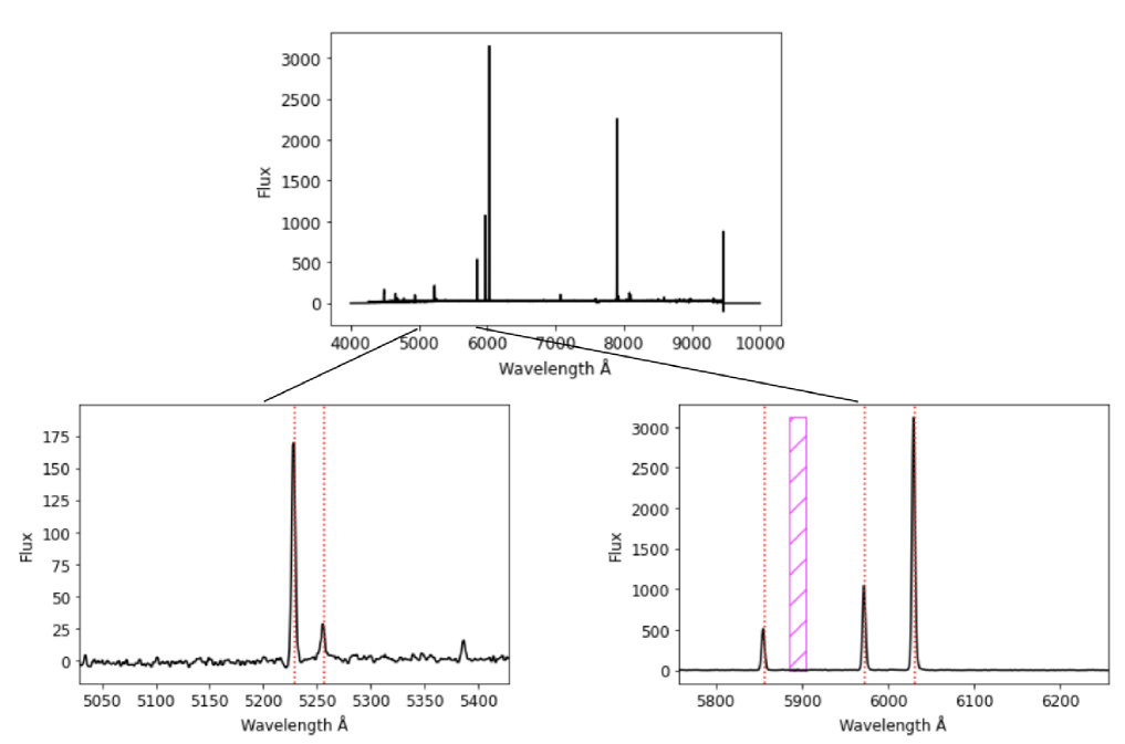
Figure 1: Example DEIMOS spectrum for a galaxy in our sample (R.A.(J$2000$)$=$3 32 41.8, Decl.(J$2000$)$=-$ 28 11 25.10, and $z=0.2044$). (Top) Complete spectrum. (Bottom left) Portion of spectrum covering H$\gamma$ and [OIII]$\lambda 4363$. (Bottom right) Portion of spectrum covering H$\beta$, [OIII]$\lambda 4959$, and [OIII]$\lambda 5007$. The red dotted lines correspond to the wavelengths of the lines at the measured redshift. The pink hatched region marks the location of a sky line. The flux units are arbitrary, as the DEIMOS spectra are not photometrically calibrated.

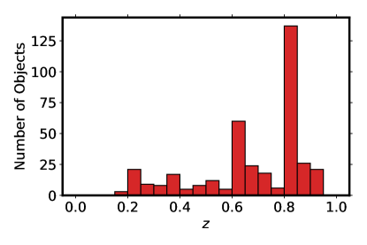
Figure 2: Redshift distribution for our high EW sample (EW₀(H$\beta)>30$ Å) of 380 galaxies. The bin width is $0.05$ in redshift. The large excess present at $z=0.63$ and $z=0.83$ is due to overlap of H$\beta$ and [OIII]$\lambda 5007$ in the narrowband filters NB816 and NB921, respectively.

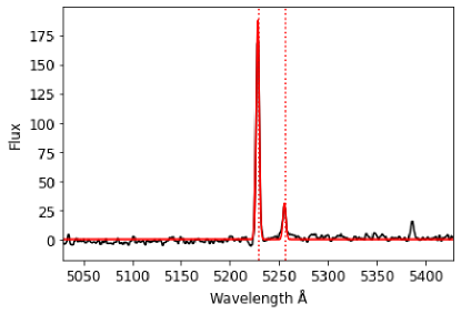
Figure 3: H$\gamma$ and [OIII]$\lambda 4363$ emission line fit for the example galaxy in Figure 1. The red curve shows the fitted model that the EWs are determined from. The red dotted lines show the means of the fitted Gaussians.

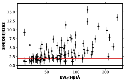
Figure 4: S/N of [OIII]$\lambda 4363$ vs. EW₀(H$\beta$) for all the sources in our sample where H$\beta$ is detected above a S/N of 20. The red line shows a S/N of 2 in [OIII]$\lambda 4363$.

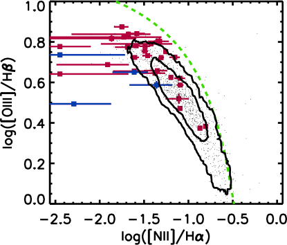
Figure 5: BPT diagram for all the sources in our sample where the H$\alpha$ line is on the spectrum and detected above a S/N of 20. The number density contours show the locus determined from the SDSS spectral sample. The dots show a subset of the SDSS data points. The green dashed curve shows the Kauffmann et al. (2003) separation between SFGs and AGNs. The red and blue points represent galaxies in our sample with $\rm 12+\log(O/H)>7.65$ and $\rm 12+\log(O/H)\leq 7.65$, respectively.

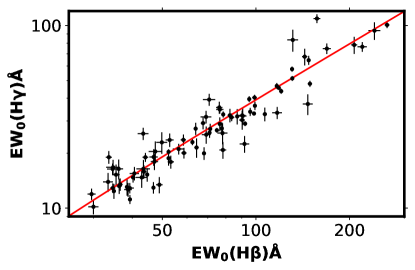
Figure 6: EW₀(H$\gamma$) vs. EW₀(H$\beta$) for all the sources in our sample where H$\beta$ is detected above a S/N of 20. The Balmer decrement is shown by the red line, assuming the underlying continuum is flat in $f_{\nu}$.

3 Analysis

3.1 EW Measurements

To determine the metallicities of our sample, we measure the EWs of the emission lines of interest in each spectrum: [OII]$\lambda 3727$, [OIII]$\lambda 4363$, [OIII]$\lambda 5007$, and [NII]$\lambda 6583$, as well as H$\gamma$, H$\beta$, and H$\alpha$. We use EWs instead of emission line fluxes to avoid introducing biases from spectral flux calibrations. A challenge with determining EWs is measuring the continua of the spectra. We carefully inspected the spectra of all the sources with very weak continua to make sure that the continua are plausible. However, since we are primarily concerned with local line ratios, a continuum measurement is not critical to the metallicity determination. To measure the EWs, we simultaneously fit Gaussian functions to neighboring emission lines of interest, and we divide the integrated area under each fitted Gaussian by the median continuum level near each line. To convert these observed-frame EWs to rest-frame EWs, we divide by $(1+z)$.

When fitting H$\beta$ and the [OIII]$\lambda\lambda 4959,5007$ doublet, we enforce a 3:1 internal ratio for the doublet and require that all three lines have the same line width. We fit a single redshift and assume that the FWHM is the same for all three lines. We fit the lines simultaneously using four free parameters ($z$, FWHM, and the amplitudes of the [OIII]$\lambda 5007$ and H$\beta$ lines). We use the same procedure to fit simultaneously the H$\alpha$ line and the [NII]$\lambda\lambda 6548,6583$ doublet. We also use similar procedures to fit two Gaussian functions, with a single FWHM and redshift, to the H$\gamma$ and [OIII]$\lambda 4363$ lines, as well as to the [OII]$\lambda\lambda 3729,3727$ doublet. We do not account for stellar absorption in the Balmer lines. Given the strength of the emission lines in EELGs, the effects of stellar absorption are extremely small.

By fitting multiple Gaussians simultaneously rather than individual lines independently, we increase the fidelity of the fits to weaker emission features. For example, [OIII]$\lambda 4363$ is a relatively weak line compared to the neighboring H$\gamma$ line. However, by simultaneously fitting H$\gamma$ and [OIII]$\lambda 4363$, we can infer the line center and line width from the stronger H$\gamma$ line, thereby improving the fit to the weaker [OIII]$\lambda 4363$ line. In Figure 3, we show the emission line fit for the example galaxy shown in Figure 1.

Selecting EELGs increases the likelihood of getting [OIII]$\lambda 4363$ detections. In Figure 4, we show all of the sources in our sample where H$\beta$ is detected above a S/N of 20. For EW₀(H$\beta$)$>50$ Å, 46 of the 70 sources are detected above a $2\sigma$ level in the [OIII]$\lambda 4363$ line. For EW₀(H$\beta$)$>100$ Å, only 4 of the 22 sources do not have $>2\sigma$ detections in [OIII]$\lambda 4363$, and most sources have a very strong detection.

In Figure 5, we show a Baldwin, Phillips, & Terlevich (BPT) diagram (Baldwin et al., 1981) for the lower redshift sources in our sample that have H$\alpha$ measurements. We require S/N $>20$ in H$\alpha$ to choose sources where we can make a robust measurement of [NII]/H$\alpha$. We compare with the locus determined by the SDSS spectral sample. The figure demonstrates that our EW measurements are robust and that we have a spectral sample of SFGs that follow the BPT track. Although Figure 5 is limited to lower redshift sources due to the spectral coverage of [NII] and H$\alpha$, our higher redshift sources also do not show active galactic nucleus (AGN) signatures, such as $\rm[NeV]\lambda 3426$. This suggests relatively little AGN contamination in the higher redshift part of the sample.

3.2 Flux Determinations

To convert the [OIII]$\lambda 5007$ to [OIII]$\lambda 4363$ EW ratio to a flux ratio, we use the relation

$$\frac{f{\rm(\lambda 5007})}{f{\rm(\lambda 4363)}}=\frac{\rm EW(\lambda 5007)}{\rm EW(H\beta)}\times\frac{\rm EW(H\gamma)}{\rm EW(\lambda 4363)}\times\frac{f(H\beta)}{f(H\gamma)}\,.$$ (1)

We assume the extinction in the sources is low and fix the flux ratio of H$\gamma$ to H$\beta$ at the Balmer decrement value of 0.47 (e.g., Osterbrock 1989). We also assume the continuum is flat between adjacent lines.

We may also compute flux ratios by assuming a shape for the underlying continuum. In Figure 6, we plot EW₀(H$\gamma$) versus EW₀(H$\beta$) for sources with H$\beta$ S/N $>20$. There is a near linear relation. Assuming the underlying continuum is flat in $f_{\nu}$ gives a median flux ratio for H$\gamma$ to H$\beta$ of 0.465, consistent with the Balmer decrement, which is shown by the red line. We use this method to compute the flux ratio of the combined [OII]$\lambda\lambda 3729,3727$ doublet to the H$\beta$ line. We consider this method more uncertain than the Balmer decrement method, which we use for the other line ratios.

3.3 Electron Temperature and Oxygen Abundance Determinations

In the $T_{e}$ method, the metallicities of galaxies are deduced from the flux ratio of the [OIII]$\lambda\lambda 4959,5007$ doublet to the [OIII]$\lambda 4363$ thermal line. We follow the prescription of Izotov et al. (2006) and use their Equations 1 and 2 to determine the electron temperatures.

Using the $T_{e}$ method also allows ion abundances for galaxies to be derived directly from the strength of the emission lines, specifically O/H. Izotov et al. (2006) empirically fit relations to an electron temperature range for common galactic emission lines. This results in a large number of ionic abundance relations, including the desired O⁺ and O²⁺ relations for this work (their Equations 3 and 5). To obtain the total abundance of Oxygen for each galaxy, these two equations must be added together. Note that there is typically little change in the total metallicity when adding O⁺ to O²⁺, as O²⁺ is the strongly dominant ionization state of Oxygen in these galaxies. This means any uncertainties in our conversion of the EW ratio to flux ratio for [OII]$\lambda 3727$/H$\beta$ are less important.

3.4 Error Analysis

We first calculated the errors on the multi-Gaussian continuum fits. For each group of simultaneously fit emission lines, we shifted the positions of the fitted lines along the spectra in regular intervals, refitting the emission lines at each interval and calculating EWs. We then took the standard deviations of these EW measures as the $1\sigma$ error bounds on the EWs of the lines. We used this method in order to properly sample the systemic, non-uniform noise in the spectra resulting from sky subtraction procedures.

To propagate the measurement errors we used a Monte Carlo technique, as analytical propagation would be needlessly complex. In this technique, we evaluated the Oxygen abundance $10,000$ times, using values drawn randomly from normal distributions for the EWs of [OIII]$\lambda\lambda\lambda$5007,4959,4363 H$\beta$, H$\gamma$, and [OII]$\lambda 3727$, centered at the measured values, and with standard deviations corresponding to the $1\sigma$ errors on each value. We used the standard deviation of the distribution of total abundance for each galaxy as the $1\sigma$ error on the abundance of that galaxy. A general overview of the above error propagation procedure can be found in Andrae (2010).

4 Discussion

Following the procedures in Section 3, we determined the $12+$log O/H abundance for each galaxy in our sample with S/N $>20$ in the H$\beta$ line and detected above a $1\sigma$ threshold in [OIII]$\lambda 4363$. In Table 1, we summarize the 10 XMPGs found in this way. The two lowest metallicities are $12+$log O/H $=6.949\pm 0.091$ and $7.208\pm 0.061$ at EW₀(H$\beta$) of $169\pm 5$ Å and $264\pm 4.69$ Å, respectively. In Figure 7, we show the triple Gaussian fits to H$\beta$, [OIII]$\lambda 4959$, and [OIII]$\lambda 5007$ and the double Gaussian fits to H$\gamma$ and [OIII]$\lambda 4363$ for these two galaxies. We show the spectra of the remaining XMPGs in the Appendix, along with $z$-band images of the four XMPGs in the SSA22 field using newly reduced Subaru Hyper Suprime-Cam imaging (B. Radzom et al. 2022, in preparation).

A majority of our objects have been identified in previous work. However, our present spectroscopic observations are significantly improved over those observations and allow for the detection of the [OIII]$\rm\lambda 4363$ Å line. Thus, our metallicity measurements for most of the objects are new. Two of our objects had previous metallicity measurements determined by Kakazu et al. (2007). In one case (2^h 40^m 35.56^s, $-1^{\circ}$ $35^{{}^{\prime}}$ $37.1^{{}^{\prime\prime}}$), the present 5 hr exposure is comparable to the 4 hr exposure used in Kakazu et al. (2007). In the other case (22^h 19^m 06.30^s, $+0^{\circ}$ $47^{{}^{\prime}}$ $21.6^{{}^{\prime\prime}}$), the present 7 hr exposure is considerably longer than the 1 hr exposure used in Kakazu et al. (2007), and the errors are correspondingly lower. We include in Table 1, if available, the original source identification and the original metallicity determination.

Table 1: All 10 XMPGs Discovered from the Final Spectral Sample of 380 Galaxies

R.A.	Decl.	$z_{spec}$	EW0(Å)					$12+$ log(O/H)	Field	Exp
(J2000.0)			H$\gamma$	[OIII]$\lambda 4363$	H$\beta$	[OIII]$\lambda 4959$	[OIII]$\lambda 5007$			(hr)
(1)	(2)	(3)	(4)	(5)	(6)	(7)	(8)	(9)	(10)	(11)
22 17 46.38†	+0 18 13.0	0.8183	$74.743\pm 4.939$	$41.609\pm 3.789$	$169.075\pm 5.004$	$217.107\pm 10.03$	$651.32\pm 10.023$	$6.949\pm 0.092$	SSA22	19
22 19 06.30††	+0 47 21.6	0.8175	$100.766\pm 3.98$	$40.377\pm 2.987$	$264.084\pm 4.676$	$328.585\pm 6.434$	$985.756\pm 7.554$	$7.208\pm 0.061$	SSA22	7
12 37 31.51∗	+62 10 6.0	0.1724	$16.402\pm 1.933$	$8.704\pm 1.853$	$43.443\pm 2.155$	$78.84\pm 1.691$	$236.521\pm 1.618$	$7.326\pm 0.18$	HDFN	1
02 41 31.81†	-1 33 14.8	0.3930	$67.517\pm 7.056$	$13.113\pm 4.359$	$143.494\pm 2.8$	$149.177\pm 2.6$	$447.532\pm 4.029$	$7.333\pm 0.263$	XMM-LSS	17
22 17 45.40†	+0 28 18.4	0.6175	$20.41\pm 2.757$	$8.17\pm 2.545$	$47.439\pm 2.255$	$72.363\pm 4.052$	$217.09\pm 3.099$	$7.338\pm 0.256$	SSA22	6
02 40 35.56††	-1 35 37.1	0.8206	$22.911\pm 3.094$	$12.276\pm 2.355$	$49.809\pm 2.001$	$102.334\pm 1.795$	$307.002\pm 1.967$	$7.445\pm 0.167$	XMM-LSS	5
03 34 09.78≀	-28 1 28.0	0.8540	$93.78\pm 10.37$	$38.336\pm 7.321$	$240.602\pm 10.555$	$393.776\pm 12.252$	$1181.328\pm 14.547$	$7.477\pm 0.157$	CDFS	5
10 44 51.69	+59 4 22.5	0.2295	$20.815\pm 2.178$	$5.28\pm 5.025$	$78.292\pm 1.951$	$116.64\pm 5.454$	$349.92\pm 2.273$	$7.554\pm 0.551$	Lockman	1
22 17 27.33†	+0 11 50.5	0.3954	$12.849\pm 3.351$	$3.086\pm 1.567$	$44.97\pm 1.518$	$70.539\pm 2.211$	$211.618\pm 1.789$	$7.61\pm 0.455$	SSA22	10
10 33 03.85	+57 58 13.6	0.3370	$12.965\pm 3.511$	$2.403\pm 1.762$	$42.458\pm 1.812$	$54.751\pm 1.233$	$164.252\pm 1.314$	$7.647\pm 0.547$	Lockman	2

Note. — Right ascension is given in hours, minutes, and seconds, and declination is given in degrees, arcminutes, and arcseconds. ^†Identified in Kakazu et al. (2007). ^††Objects with direct $\rm T_{e}$ metallicity determinations in Kakazu et al. (2007). The respective metallicities are $12+$ log(O/H) $=7.43\begin{subarray}{c}+0.18\\ -0.15\end{subarray}$ and $12+$ log(O/H) $=7.43\begin{subarray}{c}+0.22\\ -0.17\end{subarray}$. ^∗Identified in Ashby et al. (2015) ^≀Identified in Wold et al. (2014).

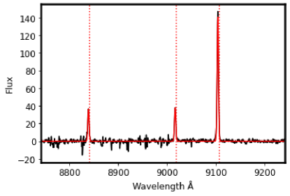
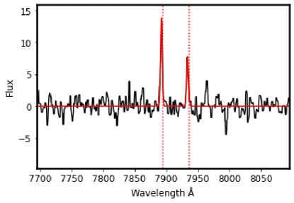
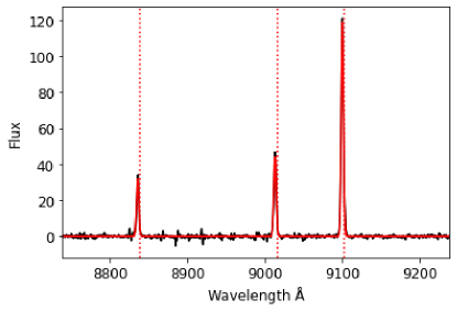
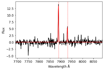
Figure 7: Left: Emission lines H$\beta$, [OIII]$\lambda 4959$, and [OIII]$\lambda 5007$ in the (top) lowest metallicity galaxy with $12+$log O/H $=6.949\pm 0.091$ and (bottom) second lowest metallicity galaxy with $12+$log O/H $=7.208\pm 0.061$, along with their triple Gaussian fits. Right: Emission lines H$\gamma$ and [OIII]$\lambda 4363$ for the same two galaxies, along with their double Gaussian fits. A 5-point median smoothing has been applied.

In Figure 8 we show $12+$log O/H abundance versus EW₀(H$\beta$). Those galaxies not detected above $1\sigma$ in [OIII]$\lambda 4363$ are shown at a nominal (high) value of 10. In examining the figure, a relation can be seen between $12+$log O/H and EW₀(H$\beta$). Specifically, as EW₀(H$\beta$) increases, the metallicity decreases with a median metallicity of 8.39 for sources with EW${}_{0}=50-100$ Å and 8.07 for sources with EW${}_{0}>100$ Å. For the EW${}_{0}\geq 100$ Å region, a Pearson’s correlation test gives a linear correlation factor (r-value) of $-0.51$ and a probability value of $0.02$ for an uncorrelated system to produce the same r-value.

A simple linear fit between the O abundances and $\log$ EW₀(H$\beta$) gives the relation

$$12+\rm{log(O/H)}=12.810\pm 0.101\\ -2.233\pm 0.061\times\log\rm EW_{0}(H\beta)~{}\AA$$ (2)

for galaxies with EW${}_{0}\geq 100$ Å (black curve). We determined the errors on the fit by performing a Monte Carlo simulation based on the uncertainties in the EW₀($H\beta$) and metallicity of the dataset. We show the $1\sigma$ distribution of the resulting set of fits in green shading in Figure 8. The minimum EW₀(H$\beta$) requirement ensures the fitted relation accurately represents the higher EW₀(H$\beta$) lower metallicity region, which has been under-constrained in past XMPG surveys. This relation underlines the effectiveness of searching for XMPGs in samples of high-EW emission-line galaxies. To highlight the high-EW sample we focus on subsequently, we plot the data points at EW₀(H$\beta)<100$ Å with fainter symbols, and we plot a vertical line at EW₀(H$\beta)=100$ Å.

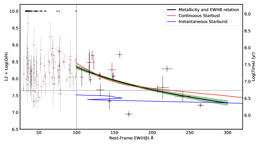
Figure 8: EW₀(H$\beta$) vs. metallicity for our sample with S/N cuts of H$\rm\beta\geq 20$ and [OIII]$\lambda 4363$ $\geq 1$. Data that met the S/N cut of H$\beta\geq 20$ but not [OIII] $\lambda 4363$ $\geq 1$ are plotted at a nominal value of $10$. Prior EW₀(H$\rm\beta$) vs. metallicity plots suffered from a lack of galaxies populating the region where EW₀(H$\beta$) exceeded $\rm 100~{}\AA$, and thus the overall shape of the relation was under-constrained. Here we see that as the rest-frame EW increases, the metallicity decreases. The black vertical dotted line shows the low metallicity threshold of $12+$log (O/H)$=7.65$, which is $1/10$th of the solar metallicity. The black solid curve represents a linear fit of $12+\rm{log(O/H)}=12.810\pm 0.101-2.233\pm 0.061\times\log\rm EW_{0}(H\beta)~{}\AA$. We show the $\rm 1\sigma$ distribution of the Monte Carlo simulation fits in green shading. The metallicity abundance error and EW₀(H$\beta$) error were determined from the procedures presented in Section 3.4. Also shown are the continuous (red curve) and instantaneous (blue curve) starburst models from Starburst99. We plot the data points at EW₀(H$\beta)<100$ Å with fainter symbols and change each starburst model curve to dotted. We plot the XMPG sample as a different symbol to differentiate between our high metallicity and low metallicity sample. There is agreement between the metallicity and EW₀(H$\beta$) relation and the continuous starburst model at high EWs, which underlines the dependence of metallicity and EW₀(H$\beta$) on age.

We are interested in the relationships between EW₀(H$\beta$), metallicity, and galaxy age (t) at EW₀(H$\beta)\geq 100$ Å; specifically, the EW₀(H$\beta$) evolution and the changes in metallicity as a function of galaxy age. By galaxy age, we mean the time since the onset of the currently dominant star formation episode. This does not preclude there being older underlying populations in the galaxy. To determine these relationships, we must first assume a star formation model.

We constructed instantaneous and continuous starburst models using the program Starburst99 (Leitherer et al., 1999; Vázquez & Leitherer, 2005; Leitherer et al., 2010, 2014). We left the initial parameters for each Starburst99 model unchanged. We show the models in Figure 9.

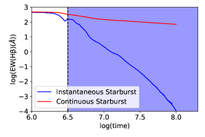
Figure 9: EW(H$\beta$) vs. time for the instantaneous (blue curve) and continuous (red curve) starburst models from Starburst99. The shaded region represents the time region of each model where we fit the models.

In Figure 8, we see that the instantaneous starburst model, where the EW(H$\beta$) drops very rapidly with time, is a poor fit to our data at EW₀(H$\beta$)$\geq 100$ Å; thus, we focus our attention on the continuous starburst model. Specifically, we fit a power law to the continuous starburst model for $\rm t>10^{7}$ yr, which gives the relation

$$\rm\log t(\rm yr)=12.956-2.700\times\log\rm EW(H\beta)\,.$$ (3)

In addition to our assumption that our galaxies are undergoing continuous starburst, we assume that (1) the oxygen abundance increases linearly with time, and (2) the hydrogen abundance remains constant throughout time. With these assumptions, we obtain the following relation between metallicity and age:

$$12+\log\rm O/H=\delta+\log t(yr)\,,$$ (4)

or, combining with Equation 3,

$$12+\log\rm O/H=\delta+12.956-2.700\times\log\rm EW_{0}(H\beta)\,,$$ (5)

where $\delta$ is a single fitted parameter, which is a measure of the yield.

We overplot Equation 5 on the distribution of galaxy metallicities for $\delta=$0.93, which we chose to match the EW₀(H$\beta)\geq 100$ Å points (red curve). The blue curve is the instantaneous starburst model with the $\delta$ offset set to an arbitrary value. This curve is too flat to provide a fit to the data at EW₀(H$\beta)\geq 100$ Å.

The continuous starburst model shows reasonable agreement with the EW₀(H$\beta)\geq 100~{}$Å data, but it over-predicts the EW₀(H$\beta)<100$ Å data, suggesting that the effective yield or the specific star formation rate is dropping with time. However, Figure 8 supports the main point, which is that there is a clear relation between EW₀(H$\beta$), age, and metallicity for EW₀(H$\beta)\geq 100~{}$Åand that young XMPGs are undergoing star formation rates that are closer to continuous rather than instantaneous. Thus, for a galaxy with a measured EW₀(H$\beta$)$\geq 100$ Å, we can estimate the galaxy’s age and the galaxy’s metal abundance using Equations 3 and 5.

The models we test here do not exhaust the full range of possible parameter space of Starburst99, and thus do not cover the full scope of star formation histories. Nonetheless, the continuous starburst model fits our high-EW sample well. The relation between EW₀(H$\beta$) and metallicity is present due to the underlying relation of the two with the age of the galaxy.

In summary, we show that for EW₀(H$\beta$)$\geq 100$ Å, EW₀(H$\beta$) is a good proxy for galaxy age and metallicity, and XMPGs are best modeled by continuous starburst models.

5 Summary

In this study, we discovered 8 new galaxies below the XMPG threshold of $12+\log$ O/H $=7.65$ and improved upon metallicity measurements from Kakazu et al. (2007) for two more. Our lowest metallicity galaxy has $12+$log O/H $=6.949\pm 0.091$. We compared metallicity and EW₀(H$\beta$) for our spectral sample and found that at EW₀(H$\beta$)$\geq 100$ Å, there is a clear relation between the two, which we interpret as being a consequence of a near continuous star formation rate in the galaxy. For these sources, EW₀(H$\beta$) is an adequate proxy for galaxy age and metallicity.

With the spectroscopic sample sizes continually increasing, we expect to find even lower metallicity galaxies, which will help determine if there is a minimum galaxy metallicity in a given redshift range.

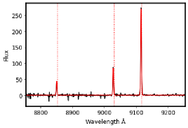
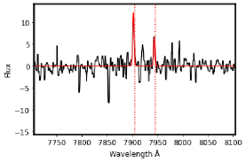
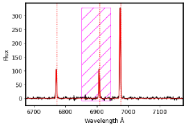
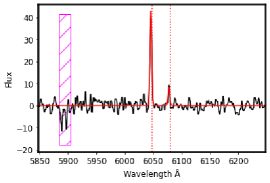
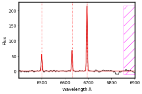
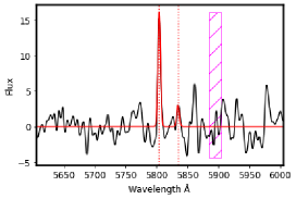
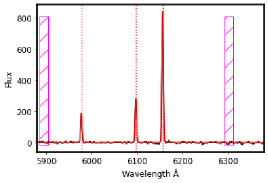
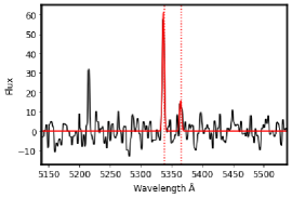
Figure 10: Left: Emission lines H$\beta$, [OIII]$\lambda 4959$, and [OIII]$\lambda 5007$ for our XMPGs with increasing metallicity, as presented in Table 1 and starting with the third source, along with their triple Gaussian fits. Right: Emission lines H$\gamma$ and [OIII]$\lambda 4363$ for the same galaxies, along with their double Gaussian fits. A 5-point median smoothing has been applied.

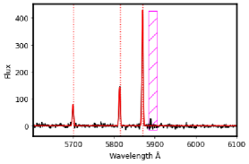
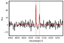
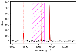
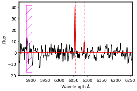
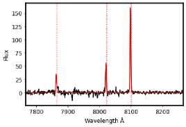
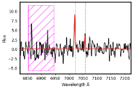
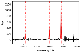
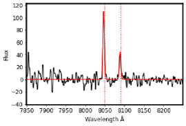
Figure 10: (Cont).

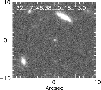
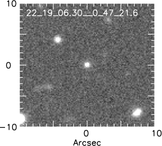
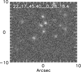
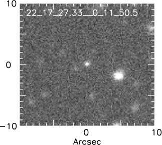
Figure 11: $\rm 20\arcsec$ x $\rm 20\arcsec$ newly reduced Subaru Hyper Suprime-Cam z-band imaging of our four XMPGs in the SSA22 field (B. Radzom et al. 2022, in preparation). As expected with high quality imaging of XMPGs, we observe a sample of compact galaxies, which matches the morphology observed in other XMPG studies (e.g., Izotov et al., 2005, 2018; Hsyu et al., 2018; Kojima et al., 2020).

References

- Amorín et al. (2014) Amorín, R., Sommariva, V., Castellano, M., et al. 2014, A&A, 568, L8
- Amorín et al. (2015) Amorín, R., Pérez-Montero, E., Contini, T., et al. 2015, A&A, 578, A105
- Andrae (2010) Andrae, R. 2010, Error estimation in astronomy: A guide
- Ashby et al. (2015) Ashby, M. L. N., Willner, S. P., Fazio, G. G., et al. 2015, ApJS, 218, 33
- Asplund et al. (2006) Asplund, M., Grevesse, N., & Jacques Sauval, A. 2006, Nuclear Physics A, 777, 1–4
- Astropy Collaboration et al. (2013) Astropy Collaboration, Robitaille, T. P., Tollerud, E. J., et al. 2013, A&A, 558, A33
- Astropy Collaboration et al. (2018) Astropy Collaboration, Price-Whelan, A. M., Sipőcz, B. M., et al. 2018, AJ, 156, 123
- Baldwin et al. (1981) Baldwin, J. A., Phillips, M. M., & Terlevich, R. 1981, Publications of the Astronomical Society of the Pacific, 93, 5
- Barger et al. (2008) Barger, A. J., Cowie, L. L., & Wang, W. 2008, The Astrophysical Journal, 689, 687–708
- Barger et al. (2012) Barger, A. J., Cowie, L. L., & Wold, I. G. B. 2012, ApJ, 749, 106
- Cardamone et al. (2009) Cardamone, C., Schawinski, K., Sarzi, M., et al. 2009, MNRAS, 399, 1191
- Cowie et al. (2016) Cowie, Barger, A. J., & Songaila, A. 2016, The Astrophysical Journal, 817, 57
- Cowie & Barger (2008) Cowie, L. L., & Barger, A. J. 2008, ApJ, 686, 72
- Cowie et al. (2004) Cowie, L. L., Barger, A. J., Hu, E. M., Capak, P., & Songaila, A. 2004, AJ, 127, 3137
- Cowie et al. (1996) Cowie, L. L., Songaila, A., Hu, E. M., & Cohen, J. G. 1996, AJ, 112, 839
- Faber et al. (2003) Faber, S. M., Phillips, A. C., Kibrick, R. I., et al. 2003, in Society of Photo-Optical Instrumentation Engineers (SPIE) Conference Series, Vol. 4841, Instrument Design and Performance for Optical/Infrared Ground-based Telescopes, ed. M. Iye & A. F. M. Moorwood, 1657–1669
- Hoyos et al. (2005) Hoyos, C., Koo, D. C., Phillips, A. C., Willmer, C. N. A., & Guhathakurta, P. 2005, ApJ, 635, L21
- Hsyu et al. (2018) Hsyu, T., Cooke, R. J., Prochaska, J. X., & Bolte, M. 2018, ApJ, 863, 134
- Hu et al. (2009) Hu, E. M., Cowie, L. L., Kakazu, Y., & Barger, A. J. 2009, ApJ, 698, 2014
- Izotov et al. (2021) Izotov, Y. I., Guseva, N. G., Fricke, K. J., et al. 2021, A&A, 646, A138
- Izotov et al. (2006) Izotov, Y. I., Stasińska, G., Meynet, G., Guseva, N. G., & Thuan, T. X. 2006, Astronomy and Astrophysics, 448, 955–970
- Izotov et al. (2005) Izotov, Y. I., Thuan, T. X., & Guseva, N. G. 2005, The Astrophysical Journal, 632, 210–216
- Izotov et al. (2018) Izotov, Y. I., Thuan, T. X., Guseva, N. G., & Liss, S. E. 2018, MNRAS, 473, 1956
- Kakazu et al. (2007) Kakazu, Y., Cowie, L. L., & Hu, E. M. 2007, ApJ, 668, 853
- Kauffmann et al. (2003) Kauffmann, G., Heckman, T. M., Tremonti, C., et al. 2003, MNRAS, 346, 1055
- Kojima et al. (2020) Kojima, T., Ouchi, M., Rauch, M., et al. 2020, The Astrophysical Journal, 898, 142
- Leitherer et al. (2014) Leitherer, C., Ekström, S., Meynet, G., et al. 2014, ApJS, 212, 14
- Leitherer et al. (2010) Leitherer, C., Ortiz Otálvaro, P. A., Bresolin, F., et al. 2010, ApJS, 189, 309
- Leitherer et al. (1999) Leitherer, C., Schaerer, D., Goldader, J. D., et al. 1999, ApJS, 123, 3
- Liang et al. (2007) Liang, Y. C., Hammer, F., Yin, S. Y., et al. 2007, Astronomy and Astrophysics, 473, 411–421
- Ly et al. (2014) Ly, C., Malkan, M. A., Nagao, T., et al. 2014, ApJ, 780, 122
- Nakajima et al. (2022) Nakajima, K., Ouchi, M., Xu, Y., et al. 2022, arXiv e-prints, arXiv:2206.02824
- Osterbrock (1989) Osterbrock, D. E. 1989, Astrophysics of gaseous nebulae and active galactic nuclei (University Science Books)
- Pagel et al. (1992) Pagel, B. E. J., Simonson, E. A., Terlevich, R. J., & Edmunds, M. G. 1992, MNRAS, 255, 325
- Pilyugin & Thuan (2005) Pilyugin, L. S., & Thuan, T. X. 2005, ApJ, 631, 231
- Rosenwasser et al. (2022) Rosenwasser, B. E., Taylor, A. J., Barger, A. J., et al. 2022, ApJ, 928, 78
- Salzer et al. (2009) Salzer, J. J., Williams, A. L., & Gronwall, C. 2009, The Astrophysical Journal, 695, L67
- Salzer et al. (2020) Salzer, J. J., Feddersen, J. R., Derloshon, K., et al. 2020, AJ, 160, 242
- Sargent & Searle (1970) Sargent, W. L. W., & Searle, L. 1970, ApJ, 162, L155
- Seaton (1975) Seaton, M. J. 1975, MNRAS, 170, 475
- Senchyna et al. (2019) Senchyna, P., Stark, D. P., Chevallard, J., et al. 2019, MNRAS, 488, 3492, doi: 10.1093/mnras/stz1907
- Vázquez & Leitherer (2005) Vázquez, G. A., & Leitherer, C. 2005, ApJ, 621, 695
- Wold et al. (2014) Wold, I. G. B., Barger, A. J., & Cowie, L. L. 2014, ApJ, 783, 119
- Wold et al. (2017) Wold, I. G. B., Finkelstein, S. L., Barger, A. J., Cowie, L. L., & Rosenwasser, B. 2017, ApJ, 848, 108
- Yin et al. (2006) Yin, S. Y., Liang, Y. C., Hammer, F., et al. 2006, Astronomy and Astrophysics, 462, 535–546