To update or not to update?
Neurons at equilibrium in deep models
Supplementary material

1 Space and time complexity evaluation

The space complexity to store the velocity term for each neuron is $\mathcal{O}(\|\Xi_{val}\|_{0}\cdot N_{i})$, but as highlighted in Sec. LABEL:sec:albation-val-eps, $\|\Xi_{val}\|_{0}$ can be extremely small, and provides comparably good results even with just a size of one. We hypothesize that this is possible thanks to the heterogeneity of features extracted from a single image: even if we have a single image as input, the sampling points for the equilibrium are a typically large number in convolutional layers. We recommend however to have one input image per class in classification tasks, and to have sufficient representation for each class in semantic segmentation tasks.

During the forward pass, the time complexity for the equilibrium computation (for the given $i$-th neuron) depends on two factors: $N_{i})$ and $\|\Xi_{val}\|_{0}$. For the computation of $\phi_{i}$, the complexity will be $\mathcal{O}(\|\Xi_{val}\|_{0}\cdot N_{i})$. For the variation of $\Delta\phi_{i}$, as it is a simple subtraction, the complexity is simply $\mathcal{O}(1)$ as well as the subtraction with the velocity term in (LABEL:eq:velocity1). We conclude that the time complexity for the equilibrium evaluation for every neuron is $\mathcal{O}(\|\Xi_{val}\|_{0}\cdot N_{i})$ (which is easily parallelizable on GPU).

2 Effect of the norm at the single neuron’s scale

In order to assess the concept of neuronal equilibrium, we normalize the output vectors to be compared, as the variation of scale at the output of a neuron can be easily re-conducted to simple amplification effects associated to the neuron’s parameters or to its input. More formally, let us consider for sake of simplicity a fully-connected layer. We define $\Delta x$ as the variation of the input of a neuron (hence, not the input of the whole model $\xi$) and $\Delta w$ as the variation of the parameters of the models. We consider here the simple case in which $\phi_{i}^{t}=0$ and $\|y_{i}^{t}\|_{2}\neq\|y_{i}^{t-1}\|_{2}$. We can write this as

$$\sum_{j}w_{i,j}^{t}\cdot x_{i,j,\xi}^{t}=\lambda\sum_{j}w_{i,j}^{t-1}\cdot x_{i,j,\xi}^{t-1},$$ (1)

where $\lambda=\frac{\|y_{i,\xi}^{t}\|_{2}}{\|y_{i,\xi}^{t-1}\|_{2}}$. We can promptly write (1) as

$$\sum_{j}(w_{i,j}^{t-1}+\Delta w_{i,j})\cdot(x_{i,j,\xi}^{t-1}+\Delta x_{i,j,\xi})=\lambda\sum_{j}w_{i,j}^{t-1}\cdot x_{i,j}^{t-1}.$$ (2)

Solving (2) for $\Delta w_{i,j}$, in the case $\lambda\neq 0$ and $\Delta x_{i,j,\xi}\neq-x_{i,j,\xi}^{t}$, we find the relation

$$\Delta w_{i,j}=\lambda\frac{w_{i,j}^{t-1}x_{i,j,\xi}^{t-1}}{x_{i,j,\xi}^{t-1}+\Delta x_{i,j}^{t-1}}.$$ (3)

From this, we identify three different cases:

• $\Delta x_{i,j,\xi}^{t-1}=0,\Delta w_{i,j}^{t-1}\neq 0$. In this case, the input of the neuron does not change, and the only change introduced is a scaling factor $\lambda$ applied to all the parameters of the neuron. As such, the input-output relationship modeled is simply scaled.

• $\Delta x_{i,j,\xi}^{t-1}\neq 0,\Delta w_{i,j}^{t-1}=0$. In this case the input is modified, but the parameters of the neuron are unchanged. (3) establishes a relationship between the variation of the parameters and the variation of the input, which must be satisfied given our hypothesis.

• $\Delta x_{i,j,\xi}^{t-1}\neq 0,\Delta w_{i,j}^{t-1}\neq 0$. In this case both the input and the parameters are modified. Also in this case, the signal intensity changes uniformly for the input, and given our hypothesis the parameters in the model can only be scaled as well: hence, the extracted output will again simply be scaled.

3 Effect of $\mu_{opt}$ in the SGD optimizer

In Sec. LABEL:sec:phi-mu, we evaluated the contribution of different values of $\mu_{eq}$, here we report the impact of another momentum term, $\mu_{opt}$, present in the SGD optimizer used to train ResNet-32 on CIFAR-10.

Fig. 1 shows the decrease in back-propagation FLOPs for different values of $\mu_{opt}$. We can observe that $\mu_{opt}=0$ leads to a sharper decrease in FLOPs (after the first learning rate decay a significant amount of neurons are frozen and remain frozen during the following epochs) at the cost of accuracy (which drops from 92.96% $\pm$ 0.21% for $\mu_{opt}=0.9$ to 91.84% $\pm$ 0.09% for $\mu_{opt}=0$). We speculate that this happens because the optimizer that uses lower $\mu_{opt}$ values, finds a (sub-optimal) local minimum and more or less remains in such minimum during the rest of the training.

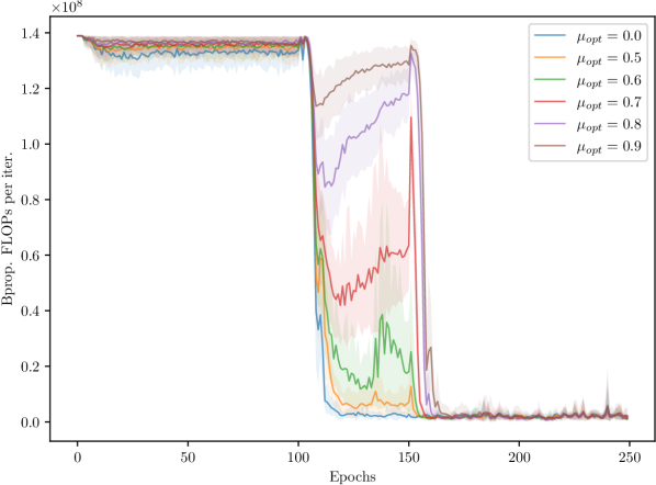
Figure 1: Back-propagation FLOPs for different values of $\mu_{opt}$.

4 Speeding up the back-propagation

Here, we provide an empirical evaluation on why avoiding the back-propagation step for a subset of neurons leads to speed-ups in the network training process.

Fig. 3 shows the execution time of the backward pass for both a fully connected and convolutional layer, for different percentages of updated neurons (denoted as $u$). For our benchmarks we used a fully connected layer with 512 input features and 1000 output features, and a convolutional layer with 64 input channels, 128 output channels, and filters of shape $3\times 3$ with an input of size 64 $\times$ 64; the reported values are averaged over 1k back-propagation iterations. We evaluate the time required for the procedure for different batch sizes.

To perform such measurements, we assume that, in each layer, the portion of neuron to update is contained in the top $u\%$ of the weight tensor. This allows us to index the target portion of the tensor in a contiguous way, avoiding major indexing overhead. Such reshuffling operation (moving the neurons indexed by NEq to the top part of the tensor) can be easily done, once per epoch, with negligible overhead. Once such prerequisite is satisfied, halting the update for the target neurons, simply just comes down to tensor slicing operations. In order to evaluate the gradients for the convolutional layer we used the high-level API provided.

Using the layers we implemented we performed some measurements of the wall-clock time with the popular ResNet-18 trained on ImageNet-1K. We have measured the wall-clock time savings at the back-propagation phase in order to compare it with the theoretical FLOPs saving. We observe a reduction in the wall-clock time: -17.52% $\pm$ 0.01% (vs the theoretical FLOP reduction -23.08% $\pm$ 0.08%). Fig. 2 shows the back-propagation execution time during training for ResNet-18 trained on ImageNet-1K.

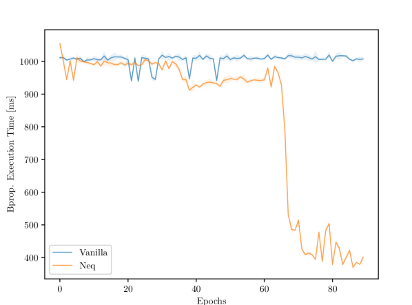
Figure 2: Back-propagation execution time for vanilla and NEq ResNet-18.

We would like to point out that our naive implementation lacks the low-level optimizations that standard PyTorch’s modules benefit from; hence, significant further improvements are possible leading to a greater time reduction, closer to the theoretical reduction. Nevertheless, we can still observe improvements when halting the update of some neurons of the layers. Developing low-level implementation of such procedure will lead to more consistent results and allow for fully exploiting NEq and is left as future work.

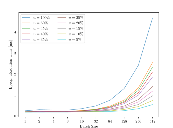
(a) Fully connected layer, size 512 $\times$ 1000.

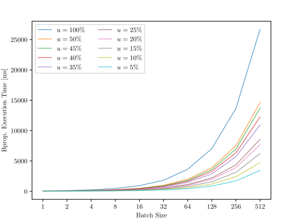
(b) Convolutional layer, size 64 $\times$ 128 $\times$ 3 $\times$ 3.

Figure 3: Back-propagation execution time for fully connected (a) and convolutional (b) layers for different batch sizes. The lower the percentage of updated neurons ($u$) the lower is the time required for the back-propagation step.

5 Additional results

In this section we provide some more insight on how NEq performs on the different learning setups shown in Sec. LABEL:sec:experiments showing that the technique adapts the the different policies. Since ResNet-32 (CIFAR-10) and ResNet-18 (ImageNet-1k) employ essentially the same learning policy, we focus on ResNet-32.

5.1 ResNet-32

Here we expand on Fig. LABEL:fig:by-epoch and Fig. LABEL:fig:distr-velocity of Sec. LABEL:sec:ablation. Figs. 5 to 20 show the distribution of $v_{\Delta\phi}$ and the FLOPs required for the back-propagation pass for all the layers of the ResNet-32 network.

The model we used in our experiments is composed by an input block of convolutional and batchnorm layers with 16 output channels, three bottleneck stages (each layer is composed by four blocks and each block with four alternating convolutional and batchnorm layers), and an output layer. The three stages have output size of 16, 32, and 64 channels, respectively.

For visualization purposes, we do not show batchnorm layers, as they follow the trend of the previous convolutional layer. The output layer is ignored since NEq is not applied to it.

Interestingly, we observe that the layers close to the input (Fig. 5) reach equilibrium immediately, and indeed we are able to block a significant part of neurons’ updates already at the early stages of the training. We speculate that, in order to allow the whole model to reach equilibrium at the end of the learning process, the layers which are close to the input must be the first to learn their input-output relationships. Indeed, if this does not happen, and they continuously change their value, their changing behavior will have an impact on all the neurons in deeper layers, driving them as well in non-equilibrium states. According to this interpretation, if we look at the layers close to the output (Fig. 20), we see indeed that they reach equilibrium very late.

5.2 Swin-B and Deeplabv3

To show how NEq automatically adapts to the training policy, Fig. 4 shows the decrease in back-propagation FLOPs during training for both the Swin-B and the Deeplabv3 architectures compared to the learning rate scheduling employed durinig training.

We can see that, for both setups, as the training progresses and the networks converge toward the equilibrium, more and more neurons are no longer updated. This shows that NEq automatically adapts to the state of the network regardless of how the training occurs.

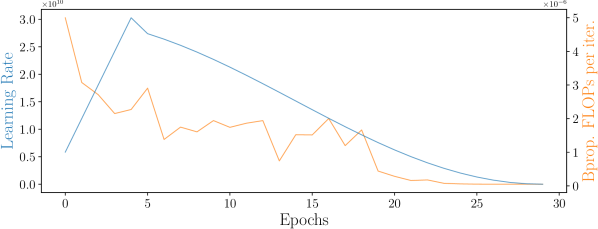
(a)

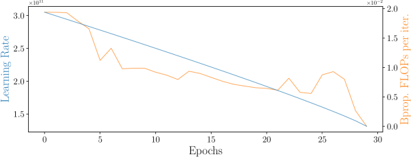
(b)

Figure 4: Decrease in back-propagation and learning rate scheduling for Swin-B (a) and Deeplabv3 (b) during training.

6 Broader impact

In the last years, deep neural networks have been one of the most studied and used algorithms for Artificial Intelligence, and they are state-of-the-art to solve a huge variety of tasks, including, but not limited to, image classification, segmentation and generation. Their success comes from their ability to automatically learn from examples, not requiring any specific expertise and using very general learning strategies. The use of GPUs for training ANNs boosted their large-scale deployability. However, this has an environmental impact, as very large computational resources are deployed, consuming relevant amounts of power. This work is not the only one finding ways to save computational power (hence, energy) for training deep learning model, and in particular that is just a benefit coming from neuronal equilibrium. Prospectively, however, NEq can enable a whole class of learning algorithms, specifically designed towards power savings, in order to achieve a positive environmental impact.

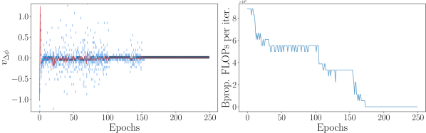
Figure 5: ResNet-32 input layer

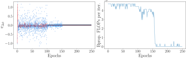
(a) Conv_a

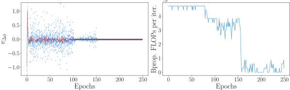
(b) Conv_b

Figure 6: ResNet-32 stage_1, 0

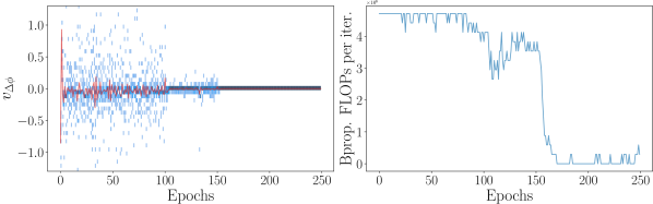
(a) Conv_a

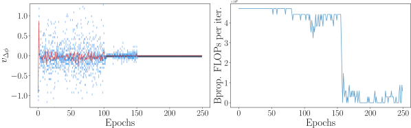
(b) Conv_b

Figure 7: ResNet-32 stage_1, 1

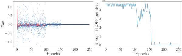
(a) Conv_a

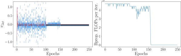
(b) Conv_b

Figure 8: ResNet-32 stage_1, 2

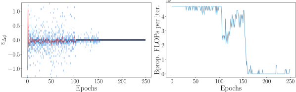
(a) Conv_a

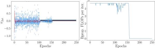
(b) Conv_b

Figure 9: ResNet-32 stage_1, 3

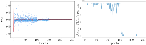
(a) Conv_a

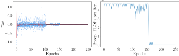
(b) Conv_b

Figure 10: ResNet-32 stage_1, 4

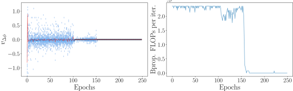
(a) Conv_a

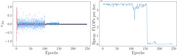
(b) Conv_b

Figure 11: ResNet-32 stage_2, 0

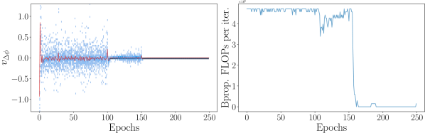
(a) Conv_a

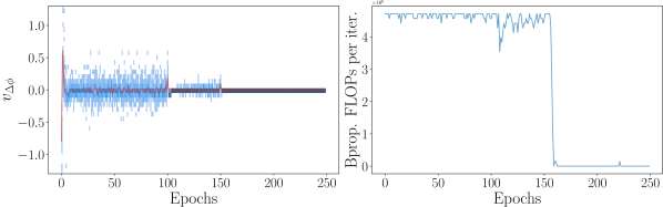
(b) Conv_b

Figure 12: ResNet-32 stage_2, 1

(a) Conv_a

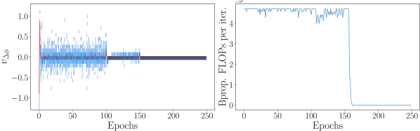
(b) Conv_b

Figure 13: ResNet-32 stage_2, 2

(a) Conv_a

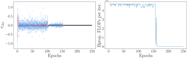
(b) Conv_b

Figure 14: ResNet-32 stage_2, 3

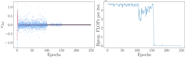
(a) Conv_a

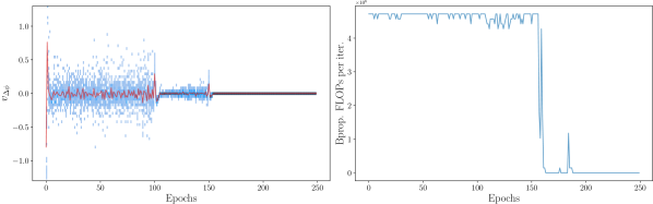
(b) Conv_b

Figure 15: ResNet-32 stage_2, 4

(a) Conv_a

(b) Conv_b

Figure 16: ResNet-32 stage_3, 0

(a) Conv_a

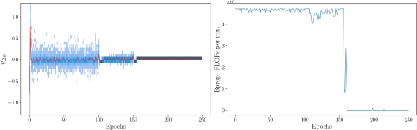
(b) Conv_b

Figure 17: ResNet-32 stage_3, 1

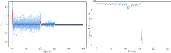
(a) Conv_a

(b) Conv_b

Figure 18: ResNet-32 stage_3, 2

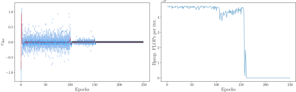
(a) Conv_a

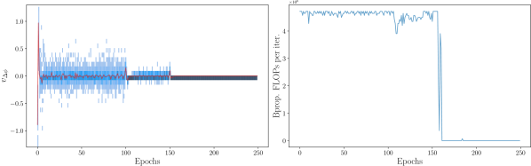
(b) Conv_b

Figure 19: ResNet-32 stage_3, 3

(a) Conv_a

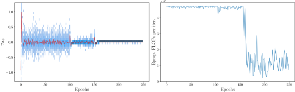
(b) Conv_b

Figure 20: ResNet-32 stage_3, 4