Maximally entangled proton and charged hadron multiplicity in Deep Inelastic Scattering

Abstract

We study the proposal by Kharzeev-Levin to determine entanglement entropy in Deep Inelastic Scattering (DIS) from parton distribution functions (PDFs) and to relate the former to the entropy of final state hadrons. We find several uncertainties in the current comparison to data, in particular the overall normalization, the relation between charged versus total hadron multiplicity in the comparison to experimental results as well as different methods to determine the number of partons in Deep Inelastic Scattering. We further provide a comparison to data based on leading order HERA PDF as well as PDFs obtained from an unintegrated gluon distribution subject to next-to-leading order Balitsky-Fadin-Kuraev-Lipatov and Balitsky-Kovchegov evolution. Within uncertainties we find good agreement with H1 data. We provide also predictions for entropy at lower photon virtualities, where non-linear QCD dynamics is expected to become relevant.

1 Introduction

Entanglement is a nonlocal correlation unique to quantum systems [1], see also the reviews [2, 3]. There are various proposals how to study entanglement in high energy physics such as neutrino oscillations, spin correlations of $t-\bar{t}$ quarks or $\Lambda$ hyperons [4, 6, 5, 7]. A measure of entanglement which is of particular interest is entanglement entropy [8]. In [9] it has been proposed that one can associate entanglement entropy with the system of partons probed in Deep Inelastic Scattering (DIS) experiments. The proposal necessarily requires a measurement process which introduces a bi-partition to the system. The measured system is no longer in a pure quantum state and as a consequence entropy arises. The proposal in [9] considers coordinate space entropy and is motivated by exact results obtained in conformal field theories in 1+1 dimensions [10, 11]. The 1+1 dimensional picture provides reasonable guidance, since the basic quantity which describes the system of partons at some resolution scale is the integrated density of partons, i.e. the parton distribution function (PDF). It provides information about the one dimensional spatial structure of protons, although the underlying dynamics may take place in transverse dimension as well. For further developments and other approaches see [14, 15, 16, 17, 18, 19, 20, 25, 26, 27, 13, 12, 28, 21, 22, 23, 24, 29, 30].

The measurement process is provided by a probe. In DIS this probe is given by the virtual photon that is exchanged between electron and proton. Since the photon probes only parts of the partonic system of the proton, the remaining part has to be integrated out or traced over, giving rise to a reduced density matrix and therefore entanglement entropy. We note that this approach was also used to estimate entanglement entropy produced in proton-proton collisions at the LHC [13]. It can be motivated as follows: for DIS at low $x$ and referring to the proton rest frame, it is possible to take color dipoles as the basic degrees of freedom. Color dipoles are color singlets and therefore natural candidates to generate entanglement entropy. The mechanism of the entanglement is the following:

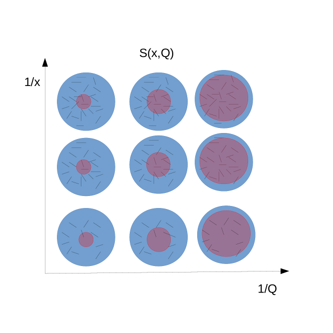
Figure 1: The figure illustrates the generation of entanglement in DIS within the dipole picture with $Q$ the photon virtuality. The blue region represents the proton, the red circle the area singled out by the virtual photon. The segments represent color dipoles in color singlet states. The entanglement arises due to dipoles that are partially in the red and blue region.

• once the virtual photon resolves substructure in the proton, it singles out a certain region of area $\sim 1/Q^{2}$ see Fig. 1.

• it might happen that one of the quarks that is a constituent of the dipole is inside the singled out region A and the other part is in the region B. Since the dipole is a color singlet state, the quark-antiquark system is strongly correlated and provides the source of entanglement between both regions. Due to the interaction, the dipole breaks up and the quark in the region B gives rise to the observed final state hadrons.

• the other quark gives a contribution to the parton distribution function measured in the DIS process

• since both constituents of the dipole were in different regions, the entropy of both regions is identical. Only dipoles that bridge the regions give rise to the observed entropy.

• as one goes to higher energies the number of dipoles increases (higher twists) and more and more dipoles are partially in region A and region B. As a consequence, entropy grows.

• turning to smaller $Q^{2}$, more and more dipoles are completely inside region A and the entropy should eventually decrease.

The framework presented in [9] provides furthermore an explicit formula on how to calculate this entanglement entropy as well as means how to obtain the latter from data through the determination of the entropy of the observed final state hadrons. Since the entire approach is based on distributions of color dipoles, which themselves can be derived from QCD within high energy factorization with $x\ll 1$ the expansion parameter, the proposed description is naturally restricted to the low $x$ regime. NLO fits of low $x$ gluon distribution are found to provide a good description of HERA data in the region $x<0.01$, see [31, 32] for a fit with the unintegrated gluon evolved with next-to-leading (NLO) Balitsky-Fadin-Kuarev-Lipatov (BFKL) evolution. The same phase space restriction $x<.01$ has been used in the fits based on leading order running coupling [33] and NLO [34] Balitsky-Kovchegov evolution, which is the non-linear low $x$ evolution equation formulated in terms of the dipole amplitude. It is therefore natural to use $x<0.01$ as an upper limit on phase space region, where the above arguments can be expected to be applicable. It is needless to say that more conservative bounds would yield even stronger justification for the underlying low $x$ approximations.

In the recent paper [35] we provided numerical evidence for this proposal, see also [36] for related work. In this way entropy at the partonic level is determined through

$$S_{\text{partonic}}\left(x,Q^{2}\right) =\ln\left[xg\left(x,Q^{2}\right)+x\Sigma\left(x,Q^{2}\right)\right],$$ (1)

where $g(x,\mu_{f}^{2})$ denotes the gluon distribution function at the factorization scale $\mu_{f}$ and $\Sigma(x,\mu_{f}^{2})=\sum_{a=1}^{n_{f}}\left(q_{a}(x,\mu^{2})+\bar{q}_{a}(x,\mu^{2})\right)$ the quark flavor singlet distribution, with $q(x,\mu^{2})$ and $\bar{q}(x,\mu^{2})$ quark and antiquark distribution functions for flavor $a$; this contribution is absent in [9] and has been added by two of us in [35]. It was further found that a framework based on the Balitsky-Fadin-Kuraev-Lipatov[37, 38, 39] (BFKL) formalism and accounting both for quarks and gluons yields satisfactory agreement with data. However, there are remaining puzzles that are still left unanswered.

From a formal point of view, the above definition and its identification with the measured hadronic entropy has the obvious shortcoming that it relates an unphysical object, i.e. scheme dependent parton distribution functions (PDFs), to an observable, i.e. hadronic entropy. From the phenomenological side, the H1 collaboration determines hadronic entropy from the multiplicities of charged charged hadrons [40]. On the other hand, the theoretical framework of [9] is based on the treatment of purely gluonic emissions which give naturally rise to both charged and neutral hadrons. Comparing therefore the prediction of [9] with data for charged hadron multiplicities, one clearly expects a certain mismatch. A related issue is the large discrepancy between partonic and hadronic entropy encountered in [40], if the former is evaluated using leading order HERA PDFs.

The outline of this paper is as follows: in Sec. 2 we provide an overview of ambiguities and open questions in the current description and how they might reflect themselves in the comparison to data. In Sec. 3 we provide updated numerical results for the BFKL description of experimental results obtained by the H1 collaboration as well as a description based on leading order HERA PDF and PDFs obtained from an unintegrated gluon distribution subject to rcBK evolution. In Sec. 4 we provide a first analysis of the transition of this framework towards a region of phase space dominated by non-linear QCD dynamics. In Sec. 5 we give our conclusions, while the appendix Sec. A summarizes details on the HSS and rcBK unintegrated gluon distribution.

2 Ambiguities in the current description

2.1 Overall normalization

The derivation of Eq. (1) is based on the expansion of the von Neumann entropy for large $y=\ln 1/x$, or equivalently low $x$ limit which is dominated by gluonic degrees of freedom. One finds

$$S_{part.} =-\sum p_{n}\ln p_{n}, p_{n}(y) =e^{-\Delta y}\left(1-e^{-\Delta y}\right)^{n-1},$$ (2)

where $p_{n}$ denotes the probability to find $n$ dipoles in the proton which satisfy $p_{1}(0)=1$ and $p_{n>1}(0)=0$. They are obtained as a solution to the following evolution equation,

$$\frac{d}{dy}p_{n}(y) =-\Delta np_{n}(y)-\Delta(n-1)p_{n-1}(y),$$ (3)

with $\Delta$ the BFKL intercept in the 2 dimensional model. Even within the 2-dimensional model, the above expression can be slightly generalized to

$$p_{n}^{gen.}(y) =Ce^{-\Delta y}\left(1-Ce^{-\Delta y}\right)^{n-1},$$ (4)

with a certain constant $C\leq 1$, which yields $p_{n}(0)\leq 1$ for all $n$. The mean number of dipoles is then obtained as

$$\langle n\rangle =\sum_{n}np_{n}=\frac{1}{C}e^{\Delta y}.$$ (5)

Given that the gluon PDF is within the 2 dimensional model subject to the BFKL equation in zero dimensions,

$$\frac{d}{d\ln 1/x}xg(x) =\Delta\cdot xg(x)$$ (6)

and taking into account that PDFs have a certain interpretation as number densities, i.e. their integral over momentum fraction $x$ yields the expectation value of the parton number operator, it is somehow natural to interpret Eq. (5) as the gluon distribution. Even though $xg(x)$ denotes usually the momentum fraction carried by gluons, while the number density is associated with the integral of $g(x)$, the above identification is correct, since one really determines the mean value of the number of partons per $\ln(1/x)$, i.e. $\langle dn/dy\rangle$, see also the more detailed discussion in Sec. 2.4.

There arises however an issue, whenever the identification of Eq. (5) as the PDF is lifted from the two dimensional model to four dimensions. While the PDF in four dimensions provides merely information about the one dimensional spatial structure of the proton, it carries an additional dependence on the factorization scale, which can be traced back to an integration over the two remaining transverse dimensions. It is this additional dependence on the factorization scale as well as the associated scheme dependence of PDFs which prohibit a direct identification of PDFs as number densities. Indeed, for renormalizable gauge theories the number density interpretation applies only to certain sum rules, i.e. the difference between the number of quarks and anti-quarks of a certain flavor, which is scheme independent, see e.g. [41] for a detailed discussion. For the gluon distribution such an interpretation may at best hold within e.g. light-cone gauge at leading order; beyond leading order, the PDF turns scheme dependent. In the light of such complication the best one can hope for is that Eq. (5) is proportional to the gluon distribution at leading order, with corresponding modifications, once higher order corrections are invoked. This observation leads us to the slightly modified relation,

$$\langle n\rangle =\sum_{n}np_{n}=C^{-1}e^{\Delta Y}=B^{-1}\cdot xg(x), xg(x)=\frac{B}{C}e^{\Delta y}.$$ (7)

with some so far undetermined parameter $B$. Assuming $B=$const. and lifting this expression to four dimensions, one would then realistically test in the comparison with data the evolution in $y=\ln 1/x$ and/or in $\ln Q^{2}$. Statements about the overall normalization should on the other hand be taken with care. Similarly the quark contribution is absent in the above expression due to the use of the purely gluonic effective 2 dimensional model. Since the low $x$ seaquark distribution is driven by the gluon, the same statement applies to the relevance of this contribution, although it is naturally to be included as long as one interprets $\langle n\rangle$ as the mean number of partons. Sticking for the moment with the gluon distribution, the above expression allows to re-express probabilities as

$$p_{n}^{gen.}(x) =\frac{B}{xg(x)}\left(1-\frac{B}{xg(x)}\right)^{n-1},$$ (8)

which finally yields the following partonic entropy,

$$S_{part.}(x) =\ln\left[\frac{xg(x)}{B}-1\right]-\frac{xg(x)}{B}\ln\left[1-\frac{B}{xg(x)}\right].$$ (9)

Note that this expression is only meaningful for $xg(x)/B>1$, which is the region where Eq. (8) yields probabilities $p_{n}\leq 1$. Expanding Eq. (9) for $xg(x)\gg 1$ and assuming $B={\cal O}(1)$, one finds

$$S_{part.}(x) =\ln\left[\frac{xg(x)}{B}\right]+1+{\cal O}\left[\frac{B}{xg(x)}\right]=\ln\left[\frac{xg(x)}{B/e}\right],$$ (10)

with $e\simeq 2.71828$ Euler’s number. While for asymptotically large $xg(x)$, the contributions due to $B,e$ might be ignored, for realistic gluon distributions in the kinematic region covered by the HERA experiments, $S_{part.}\leq 4$ and while $xg(x)\gg 1$ is satisfied, $\ln(xg)={\cal O}(1)$ and the above finite terms should be in principle kept.

2.2 Charged versus total hadron multiplicity

The above expression allows to determine partonic entropy as a function of the average number of partons in the system. It is then conjectured that the resulting partonic entropy agrees with the hadronic entropy. The latter can be obtained from the multiplicity of final state hadrons. Since the detection of neutral hadrons is experimentally challenging, this hadronic multiplicity distribution is usually determined for charged hadrons only. With pions the predominantly produced hadron species, and assuming that final state gluons turn with equal probabilities into positively, negatively, and neutral pion states, one can as a first estimate assume that the total number of produced hadrons is roughly $3/2$ times the number of charged hadrons observed in experiment. In turn, the number of gluons and possibly seaquarks which yield charged hadrons is approximate the fraction $2/3$ of the total parton number. This suggests to correct the partonic entropy by a corresponding factor,

$$S_{part.}\to S_{charged}=S_{part.}+\ln(2/3).$$ (11)

Clearly this factor is not exact, but merely an estimate of order of magnitude.

2.3 Gluon versus Quark contribution

In [9] entanglement entropy has been determined from a 2 dimensional model calculation, based on the dipole picture, which has been related to purely gluonic degrees of freedom. In a follow up study the same authors proposed in [36] to evaluate for the kinematic region covered by the HERA experiment the partonic entropy as the logarithm of the seaquark distribution. Finally, in [35], two of us proposed to evaluate partonic entropy as the logarithm of the sum of gluon and quark contribution. This treatment was motivated by the observation that the 2 dimensional gluonic model of [9] which identifies entropy as the logarithm of the average gluon number; for the complete theory, it seems therefore appropriate to generalize the average gluon number to the average number of quarks and gluons combined. While [35] managed to successfully describe HERA data, this description was plagued by several shortcomings. While the description based on the HSS gluon of [35] uses an inconsistent combination of overall normalization constants (which we correct in the subsequent numerical study, see also Sec. A for a detailed discussion), the description based on NNLO PDFs is subject to the above mentioned scheme dependence of parton distribution functions which allows for $B\neq 1$, as already point out in [35].

In the numerical study presented in Sec. 3, we show that a description based on a combination of quark and gluon contribution yields a good description of data within uncertainties if Eq. (11) is being employed, while we set $B=e$, i.e. we ignore all pre-asymptotic factors for the time being. While the observed agreement is pleasing, we believe that in the light of the above uncertainties in normalization, the main goal of the following study is the correct description of $x$ and $Q^{2}$ dependence. The latter are directly related to evolution equations, to which the underlying distributions are subject to.

2.4 Binning and comparison to data

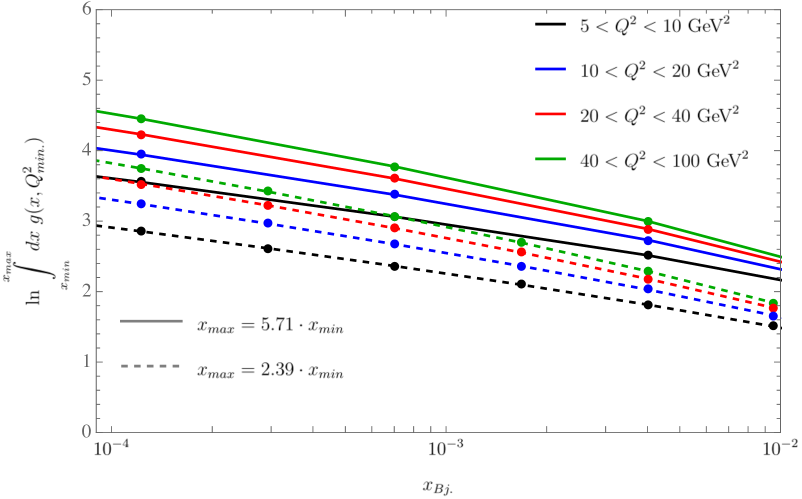
Figure 2: Partonic entropy evaluated as the logarithm of the number of gluons in a certain bin $[x_{min},x_{max}]$, see also Eq. (12) for two different bin sizes. The result clearly depends on the size of the bin. The LO HERAPDF gluon distribution is evaluated at a factorization scale corresponding to the lower $Q^{2}$ value of the $Q^{2}$ bin as in [40]

Assuming $B=e$ for the moment, and assuming $\ln(xg)\gg 1$, partonic entropy is directly determined as the logarithm of the number of partons; indeed this has been the original the proposal of [9]. In practice this can however lead to confusion, since parton distribution functions are number densities, i.e. leaving aside the above mentioned issues of scheme dependence of such distributions, one expects that the number of gluons in a proton is obtained through

$$n_{g}(Q^{2}) =\int_{0}^{1}dx\,g(x,Q^{2}),$$ (12)

with a similar expression in the case of quarks. In DIS reactions, the proton is on the other hand probed at a certain fixed value of Bjorken $x$. Experimentally this corresponds to counting final states for a certain bin size $x\in[x_{min},x_{max}]$. It is therefore tempting to define the number of gluons at a certain value of $x$ through

$$n_{g}(\bar{x}) =\int_{x_{\text{min}}}^{x_{\text{max}}}dxg(x,Q^{2}),$$ (13)

where $\bar{x}\in[x_{\text{min}},x_{\text{max}}]$ and might be defined through

$$\bar{x} =\frac{\int_{x_{\text{min}}}^{x_{\text{max}}}dx\,xg(x,Q^{2})}{\int_{x_{\text{min}}}^{x_{\text{max}}}dxg(x,Q^{2})},$$ (14)

or alternatively as the arithmetic mean of $x_{\text{min}}$ and $x_{\text{max}}$. Partonic entropy is then obtained as $\ln n_{g}(\bar{x})$. To the best of our understanding, this is the method used by the H1 collaboration to determine the partonic entropy, with $x_{max}\simeq 5.71x_{min}$, see also the determination of this quantity using this method in Fig. 2. While the method yields the number of partons in the region of phase space $[x_{\text{min}},x_{\text{max}}]$ if the PDF is interpreted as a number density, the result obviously depends strongly on the size of the interval $[x_{\text{min}},x_{\text{max}}]$. In particular the number of partons would approach zero, whenever the size of the interval turns infinitesimal small. For a meaningful comparison it is therefore necessary to study the number of partons, normalized to the bin size. Taking into account that usually one uses logarithmic bins in $x$, i.e. binning takes place in $y=\ln(1/x)$, one arrives at

$$\bar{n}_{g}(\bar{x}) =\frac{1}{y_{max}-y_{min}}\int_{y_{min}}^{y_{max}}dy\frac{dn_{g}}{dy}=\frac{n_{g}(y_{max})-n_{g}(y_{min})}{y_{max}-y_{min}}, y_{max,min}=\ln 1/x_{min,max},$$ (15)

which in the limit of infinitesimal small bin sizes leads to

$$\bar{n}_{g}(x,Q^{2}) =\frac{dn_{g}}{d\ln(1/x)}=xg(x,Q^{2}).$$ (16)

Despite of the usual association of $xg(x,Q^{2})$ with momentum sum rules, this quantity is therefore indeed the correct expression to compare to data binned in $Q^{2}$ and $Y=\ln(1/x)$. For the following numerical study, we further add the contribution due to quarks and average over the bin size in $Q^{2}$,

$$\langle\bar{n}(x,Q^{2})\rangle_{Q^{2}} =\frac{1}{Q_{\text{max}}^{2}-Q_{\text{min}}^{2}}\int_{Q^{2}_{\text{min}}}^{Q^{2}_{\text{max}}}dQ^{2}\left[xg(x,Q^{2})+x\Sigma(x,Q^{2})\right],$$ (17)

which finally yields the expression used for our comparison to data

$$\langle S(x,Q^{2})\rangle_{Q^{2}} =\ln\langle\bar{n}(x,Q^{2})\rangle_{Q^{2}}.$$ (18)

3 Numerical results

Despite the above ambiguities in the overall normalization, we believe that is meaningful to compare at the current level of accuracy theory predictions to data. Ambiguities are mainly due overall normalization constants which for the partonic entropy turn into additive constants. In the following we use three theoretical models (to be described in more detail in the Appendix):

• Leading order HERA PDF, subject to DGLAP evolution [42]. This particular set was chosen due to the observed mismatch between partonic and hadronic entropy by the H1 collaboration (which use LO HERAPDF). The goal of the comparison to LO HERAPDF is to demonstrate that such comparison should be done in the way outlined in the previous section, i.e. in bins of rapidity.

• Leading order PDFs calculated from the HSS unintegrated gluon, subject to BFKL evolution. The gluon density obtained in this scheme accounts for NLO corrections to the evolution kernel together with a collinear resummation of enhanced NLO contributions. The higher order corrections slow down the growth of the gluon density in the low $x$ region, but do not lead to saturation. The fit is limited to the region $Q^{2}>2$ GeV², see [31, 32] for details.

• Leading order PDFs calculated from an unintegrated gluon, subject to rcBK evolution. The gluon density in this framework is subject to leading order BK evolution in $x$; albeit formally leading order, the evolution kernel includes NLO resummed running coupling corrections. The evolution takes into account effects due to high gluon densities and leads to a saturated gluon density (for developments that take into account exact kinematics in combination with saturation effects see [43, 44, 45]). A description of HERA data for the proton structure function $F_{2}$ is possible, since the nonlinear term in the evolution tames the rapid growth of the gluon distribution, induced by the linear term.

The first set has been used in [40] to compare to data. We show that once the corrective factor Eq. (11) is taken into account and the number of partons is evaluated as discussed in Sec. 2.4, this set of PDFs gives actually a good description of data, in contrast to the observation made in [40], leaving aside a small off-set in the normalization, which might be traced back to the effects discussed in Sec. 2.1. The second set has been used previously in [35], while the last set is obtained from an unintegrated gluon distribution subject to Balitsky-Kovchegov (BK) evolution [47, 46] which allows us to investigate possible contributions due to non-linear QCD evolution. In all three cases we use Eq. (1) to compare to data. The contribution due to seaquarks is in general small; the normalization of the description based on leading order HERA PDFs would slightly improve if one would only consider the contribution due to the gluon.

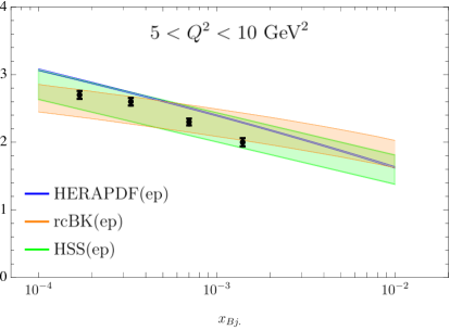
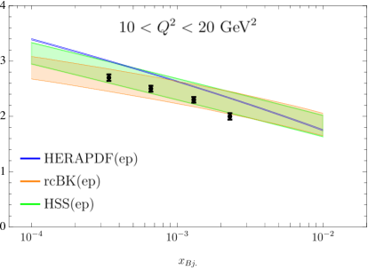
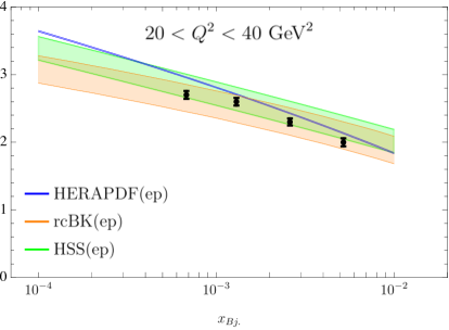
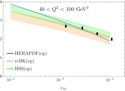
Figure 3: Partonic entropy corrected for charged hadrons only $\ln\left(xg+x\Sigma\right)+\ln(2/3)$ versus Bjorken $x$. Results are compared to the final state hadron entropy derived from the charged multiplicity distributions measured by the H1 collaboration [40] for track pseudorapidities $\eta^{*}$ in the hadronic centre-of-mass frame restricted to the range $0<\eta^{*}<4$.

To obtain entropy from the low $x$ QCD evolution equations, we need to determine PDFs i.e. integrated parton densities. The gluon density is obtained from

$$xg(x,\mu_{F}) =\int_{0}^{\mu_{F}^{2}}d{\bm{k}}^{2}{\mathcal{F}}(x,{\bm{k}}^{2}),$$ (19)

where ${\cal F}(x,{\bm{k}}^{2})$ is the unintegrated gluon distribution, which is obtained from a solution to BFKL or BK evolution equations, including a fit to data. To obtain the quark PDF we apply the Catani-Hautmann procedure [48]

$$x\Sigma(x,Q) =\int_{0}^{\infty}\frac{d{\bm{\Delta}}^{2}}{{\bm{\Delta}}^{2}}\int_{0}^{\infty}d{\bm{k}}^{2}\int_{0}^{1}dz\Theta\left(Q^{2}-\frac{{\bm{\Delta}}^{2}}{1-z}-z{\bm{k}}^{2}\right)\tilde{P}_{qg}\left(z,\frac{{\bm{k}}^{2}}{{\bm{\Delta}}^{2}}\right)\mathcal{F}(x,{\bm{k}}^{2}),$$ (20)

where the splitting function reads [48]

$$\tilde{P}_{qg}\left(z,\frac{{\bm{k}}^{2}}{{\bm{\Delta}}^{2}}\right) =\frac{\alpha_{s}2n_{f}}{2\pi}T_{F}\frac{{\bm{\Delta}}^{2}}{[{\bm{\Delta}}^{2}+z(1-z){\bm{k}}^{2}]^{2}}\left[z^{2}+(1-z)^{2}+4z^{2}(1-z)^{2}\frac{{\bm{k}}^{2}}{{\bm{\Delta}}^{2}}\right],$$ (21)

and $\mu_{F}$ denotes the factorization scale which we identify for the current study with the photon virtuality $Q$. ${\bm{k}}$ denotes the gluon transverse momentum and ${\bm{\Delta}}={\bm{q}}-z{\bm{k}}$ with ${\bm{q}}$ the $t$-channel quark transverse momentum; $T_{F}=1/2$. ${P}_{qg}(z)=\frac{\alpha_{s}2n_{f}}{2\pi}T_{F}\left[z^{2}+(1-z)^{2}\right]$. In [35] the HSS integrated gluon Eq. (19) has been determined using a version of the unintegrated gluon with an overall normalization inconsistent with the normalization used for the determination of the quark PDF. In the following numerical study this has been corrected. In more general terms, the possibility of such inconsistencies can be traced back to a relatively large uncertainty in the overall normalization of the unintegrated gluon distributions, which have been obtained through fits which rely on the use of the leading order virtual photon impact factor. Since the latter is – as the seaquark distribution – proportional to $\alpha_{s}$, it induces a relatively large normalization uncertainty on the extracted unintegrated gluon. To assess these uncertainties we multiply in the case of the HSS distributions the integrated gluon distribution by a factor $\alpha_{s}(Q^{2})/\alpha_{s}(\mu^{2})$ and vary the renormalization scale $\mu$ in the range $\mu\in[Q/2,2\cdot Q]$. The unintegrated dipole gluon density subject to rcBK evolution is obtained through

$${\cal F}(x,k^{2})=\frac{N_{c}k^{2}S_{\perp}}{8\pi^{2}\alpha_{s}}\int dr^{2}(1-N(r,x))J_{0}(r^{2}k^{2}),$$ (22)

where $N(r,x)$ is dipole amplitude obeying BK equation in coordinate space, see App. Sec. A for more details. In the above expression $\alpha_{s}$ is kept constant, while it is running in the kernel of the evolution equation. In order to obtain uncertainties we use $\alpha_{s}\in[0.2,0.3]$, which are typical values for the hard scales investigated in this study. For the description based on leading order HERA PDFs we show the relatively small leading order PDF uncertainties, making use for the numerical evaluation of the package [49].

We find in Fig. 3 that the partonic entropy Eq. (18) obtained from the total number of partons gives a still a very good description of H1 data [40]. In particular within uncertainty bands, both HSS and rcBK give a good description of data. The HERA PDFs slightly overshoot the data but not as drastically as presented in [40]. This is due to the factor $\ln(2/3)$ which corrects for the fact that only charged hadrons have been measured as well as the effects discussed in Sec. 2.4. Since gluon and quark contribution add up, the description would slightly improve without the latter.

4 Towards the real photon limit

Having described the moderate and large $Q^{2}$ data, a natural question to ask is what happens if we go to lower values of $Q^{2}$. With $1/Q^{2}$ the effective area resolved in the interaction of virtual photon and proton, the limit $Q^{2}\to 0$ naturally leads to the case where the photon would observe the entire proton; entanglement entropy should be therefore absent in this limit. While the complete description of such a scenario is still unknown, we believe that investigating this limit within the current framework is already of interest. A more complete description should be probably formulated within the more general frameworks[50, 51], where saturation effects [52] and therefore classicalization of wee gluons are taken into account [20]. For the moment we do not consider such modifications. Instead we will investigate the limit of small photon virtualities $Q^{2}$. In Fig. 4 we show entanglement entropy as obtained from the solution to the rcBK evolution equation, as well as the HSS gluon and leading order HERA PDFs. While the rise with $x$ flattens for three descriptions, this effect is clearly stronger for the rcBK description, which we attribute to effects related to gluon saturation. For leading order HERA PDFs and the HSS gluon, we limit the calculations to values $Q^{2}>1$ GeV² since for smaller values these descriptions would break down. This is however not a limitation for the rcBK or Golec-Biernat Wusthoff saturation model [53], which has been fitted for smaller values of $Q^{2}$. From a formal point of view, one may justify this through the presence of a semi-hard saturation scale $Q_{s}(x)>\Lambda_{\text{QCD}}$. While results for $Q^{2}<1$ GeV² must be interpreted with care, they allow for a first qualitative investigation of this region of phase space. We will proceed with analytical studies of this region using the GBW model.

 

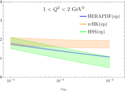
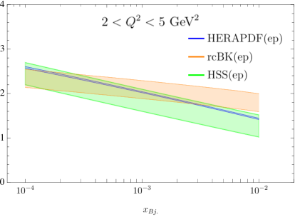
Figure 4: Partonic entropy corrected for charged hadrons only, $\ln\left(xg+x\Sigma\right)+\ln(2/3)$ versus Bjorken $x$, calculated for low $Q^{2}$ bins. The result demonstrates saturation of entropy at low $Q^{2}$ and low $x$.

 

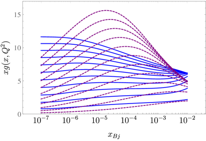
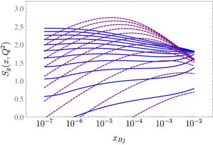
Figure 5: Gluon PDF (left) and entropy (right) from rcBK (blue continuous lines) and GBW (purple dotted lines) unintegrated gluon distributions, versus Bjorken $x$, as given by Eq. (19) and Eq. (1) (for gluons only) calculated for low $Q^{2}$ values. The result demonstrates saturation and decrease of entropy at low $Q^{2}$ and low $x$. The values are $Q^{2}=0.3$ GeV² (bottom of the plot) up to $2.3$ GeV² (top of the plot).

Within this model, the dipole unintegrated gluon density reads:

$${\cal F}(x,k^{2})=\frac{N_{c}S_{\perp}}{\alpha_{s}8\pi^{2}}\frac{k^{2}}{Q_{s}^{2}}e^{-k^{2}/Q_{s}^{2}}$$ (23)

where $Q_{s}=Q_{0}^{2}\left(\frac{x_{0}}{x}\right)^{\lambda}$. The integrated gluon distribution is then obtained as

$$xg(x,Q^{2}) =\frac{N_{c}S_{\perp}}{\alpha_{s}8\pi^{2}}\left[Q_{s}(x)^{2}\left(1-e^{Q^{2}/Q_{s}^{2}(x)}\right)-Q^{2}e^{Q^{2}/Q_{s}^{2}(x)}\right].$$ (24)

For large photon virtualities $Q^{2}\gg Q_{s}(x)^{2}$ this yields

$$\lim_{Q^{2}\gg Q_{s}^{2}}xg(x,Q^{2}) =\frac{N_{c}S_{\perp}}{\alpha_{s}8\pi^{2}}Q_{s}^{2},$$ (25)

i.e. the integrated gluon distribution is directly proportional to the saturation scale. In the limit of small photon virtualities one finds on the other hand:

$$\lim_{Q^{2}\ll Q_{s}^{2}}xg(x,Q^{2})=\frac{N_{c}}{\alpha_{s}16\pi^{2}}\frac{S_{\perp}Q^{4}}{Q_{s}^{2}(x)}\sim x^{\lambda},$$ (26)

i.e. the integrated gluon distribution turns into a falling function of $x$. In particular one has the formal limit $xg(x,Q^{2}=0)=0$. For entanglement entropy one finds, extrapolating the current framework to low $Q^{2}$,

$$\lim_{Q^{2}\ll Q_{s}^{2}}S(x,Q^{2})=\ln\left(\frac{S_{\perp}Q^{4}}{Q_{s}^{2}(x)}\right)+\ln\frac{N_{c}}{16\alpha_{s}\pi^{2}}.$$ (27)

Depending on the precise values of the transverse size $S_{\perp}$, this expression will for some value of $x$ turn eventually negative. Note however that the definition of probabilities Eq. (8) requires $xg(x)\geq B=e$, for the current setup, which prevents us from reaching negative values. On the other hand for $Q^{2}\gg Q_{s}(x)^{2}$ we have

$$\lim_{Q^{2}\gg Q_{s}^{2}}S(x,Q^{2})=\ln\left(S_{\perp}Q_{s}^{2}(x)\right)+\ln\frac{N_{c}}{8\alpha_{s}\pi^{2}}=\lambda\ln\frac{1}{x}+\text{const.},$$ (28)

i.e. we recover the original expression for partonic entropy obtained in [9] plus a certain constant contribution.

A numerical study of the GBW model compared to rcBK is provided in Fig. 5. In the figure we plot only the contributions due to gluons. Entropy is being evaluated at low values of $Q^{2}<1$ GeV² since the both gluon densities have been fitted for this region of phase space. Moreover there exist in principle data for this region of phase and a comparison to those data would be of high interest, once they are in available in a suitable form. From a formal point of view, the existence of a semi-hard saturation scale allows for the evaluation of the gluon density at such low scales. We however stress here that the entropy formula in this region is an extrapolation. As can be seen from the plot to the right, the integrated gluon distribution is no longer necessarily large at lowest values of $x$. The expansion of Eq. (9) for large $xg(x)$ is therefore not necessarily a good approximation. We therefore compare in Fig. 6 both the exact formula for entropy, derived within the 2 dimensional model, and its asymptotic expansion. The exact formula is not necessarily more accurate than the asymptotic expression, but the observed deviation indicates in which regions of phase space effects due to non-linear QCD dynamics might become relevant. In all of the the calculations we assume $B=e$ which is the choice which minimizes the contribution due to constant terms.

   

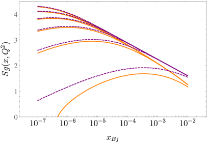
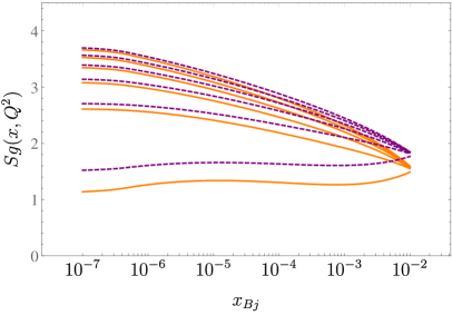
Figure 6: Left: GBW partonic entropies for increasing $Q^{2}$ from bottom to top with $Q^{2}=1$ GeV² the lowest and $Q^{2}=11$ GeV² the highest value with increments by $Q^{2}=2.5$ GeV², versus Bjorken $x$, as given by Eq. (18) (orange continuous) and Eq. (10) (purple dashed) assuming $B=e$. Right: the same as left but the integrated gluon obtained from the rcBK unintegrated gluon is used to determine entropy.

Note that the observation that for certain values of $Q^{2}$ the gluon PDF is a falling function of $x$ can be directly linked to the behavior of the dipole amplitude featuring saturation stemming from a solution to BK or JIMWLK [54, 55, 56, 57] evolution and which has been already observed for the solution of the BK equation in [58]. We interpret this as a mechanism of localization due to saturation of wee partons in longitudinal direction.

5 Conclusions

In this paper we continued the study of the proposal formulated in [9] to calculate for DIS reactions entanglement entropy from parton distribution functions. The purpose of this study has been twofold: on one hand we attempted to clarify some of the lose ends of this proposal such as the overall normalization, the relation between entanglement entropy and hadronic entropy of charged hadrons as well as a discussion on how to evaluate the number of partons for the determination of partonic entropy. On the other hand we provided a first exploration of the proposal towards low photon virtualities and very low $x$, where eventually non-linear QCD dynamics is expected to manifest itself.

To this end we provided a description of the data measured by the H1 collaboration through parton distribution functions subject to BFKL and BK evolutions equations as well as leading order HERA PDFs. As outlined in section 2, the description is at the moment mainly qualitative, due to various ambiguities in the theoretical description. In particular a precise phenomenology would require to work out an appropriate factorization of entanglement entropy into parton distribution functions and corresponding perturbative coefficients which would guarantee factorization scheme independence of the framework beyond leading order. While the frameworks used in this paper agree for moderate and large values of $Q^{2}$, we find differences between BFKL evolution and leading order PDFs on the one hand and BK evolution on the other hand, if we turn to smaller values of $Q^{2}$. In particular nonlinear dynamics, as encoded in the BK equation, suggests that entropy saturates or even decreases. On technical level we link this behavior to the feature of the BK gluon PDF which predicts a valence like gluon PDF i.e. a distribution falling as a function of $x$ at some low enough value of $x$. This behavior of entanglement entropy is expected since at very low values of $Q^{2}$ the photon virtuality is so low that the system can not be bi-partitioned and entanglement entropy needs to vanish. To provide a definite answer to those questions, a generalization of the framework discussed here is necessary; in particular to explain the observed decrease of entropy with $x$.

Appendix A Some details on the rcBK and HSS

The procedure of getting the HSS unintegrated gluon density relies on solving NLO BFKL equation with BLM prescription for scale choice, collinear improvements and fitting initial condition to HERA data [31, 32]. The rcBK is basically the LO BK equation formulated in the coordinate space and with running coupling constant included. The initial conditions are fitted [33] to HERA data [59].

• The unintegrated dipole gluon density from the BK is obtained via

  $${\cal F}(x,k^{2})=\frac{N_{c}k^{2}S_{\perp}}{8\pi^{2}\alpha_{s}}\int dr^{2}(1-N(r,x))J_{0}(r^{2}k^{2})$$ (29)

  where $N(r,x)$ is dipole amplitude obeying BK equation in the coordinate space. We use $S_{\perp}=16.4$ mb and $\alpha_{S}$ is kept constant. In order to assess normalization uncertainties due to the choice of this coupling constant, we vary it in the range [0.2-0.3]]. The BK equation reads [61]

  $$\frac{\partial N(r,Y)}{\partial Y}=\int\mathrm{d}{\vec{r_{1}}}\,K^{run}(\vec{r},\vec{r_{1}},\vec{r_{2}})(N(r_{1},Y)+N(r_{2},Y)-N(r,Y)-N(r_{1},Y)N(r_{2},Y))$$ (30)

  where, $Y=\ln(x_{0}/x)$ and $\vec{r_{2}}=\vec{r}-\vec{r_{1}}$. The kernel $K^{run}$ is given by

  $$K^{run}(\vec{r},\vec{r_{1}},\vec{r_{2}})=\frac{\alpha_{s}(r^{2})}{2\pi^{2}}N_{c}\left[\frac{r^{2}}{r_{1}^{2}r_{2}^{2}}+\frac{1}{r_{1}^{2}}\left(\frac{\alpha_{s}(r_{1}^{2})}{\alpha_{s}(r_{2}^{2})}-1\right)+\frac{1}{r_{2}^{2}}\left(\frac{\alpha_{s}(r_{2}^{2})}{\alpha_{s}(r_{1}^{2})}-1\right)\right],$$ (31)

  with

  $$\alpha_{s}(r^{2})=\frac{12\pi}{(11N_{c}-2N_{f})\ln\left(\frac{4C^{2}}{r^{2}\Lambda_{QCD}^{2}}\right)};$$ (32)

  the maximal allowed value for $\alpha_{s}$ is $\alpha_{s,max}=0.7$. The initial condition is given by McLerran-Venugopalan model [33, 63]

  $$N^{\mathrm{MV}}(r,Y=0)=1-\exp\left[-\frac{(r^{2}Q_{s0}^{2})^{\gamma}}{4}\ln\left(\frac{1}{r\Lambda_{QCD}}+\mathrm{e}\right)\right]$$ (33)

  The equation was solved by newly developed code using Runge-Kutta method and using the parameters in the fit [33] to HERA data [59]. The numerical values of the parameter read $Q_{s0}=0.165GeV$, $\gamma=1.135$, $C=2.52$, $\Lambda_{QCD}=0.241$, $N_{f}=3$, $S_{\perp}=16.4$ mb.

• The HSS gluon density follows from the BFKL evolution equation with the kernel obtained at NLL accurancy with collinear improvements [31, 32, 64]. The unintegrated gluon density reads

  $$\mathcal{F}\left(x,{\bm{k}}^{2},M\right) =\frac{1}{{\bm{k}}^{2}}\int\limits_{\frac{1}{2}-i\infty}^{\frac{1}{2}+i\infty}\frac{d\gamma}{2\pi i}\;\;\hat{g}\left(x,\frac{M^{2}}{Q_{0}^{2}},\gamma\right)\,\,\left(\frac{{\bm{k}}^{2}}{Q_{0}^{2}}\right)^{\gamma}$$ (34)

  where $M$ is a characteristic hard scale of the process which we identify with $Q$. $\hat{g}$ is an operator in $\gamma$ space,

  $$\hat{g}\left(x,\frac{M^{2}}{Q_{0}^{2}}\gamma\right) =\frac{\mathcal{C}\cdot\Gamma(\delta-\gamma)}{\pi\Gamma(\delta)}\;\cdot\;\left(\frac{1}{x}\right)^{\chi\left(\gamma\right)}\,\cdot$$

  $$\Bigg{\{}1+\frac{\bar{\alpha}_{s}^{2}\beta_{0}\chi_{0}\left(\gamma\right)}{8N_{c}}\log{\left(\frac{1}{x}\right)}\Bigg{[}-\psi\left(\delta-\gamma\right)+\log\frac{{M}^{2}}{Q_{0}^{2}}-\partial_{\gamma}\Bigg{]}\Bigg{\}}\;,$$ (35)

  where $\bar{\alpha}_{s}=\alpha_{s}N_{c}/\pi$ with $N_{c}$ the number of colors and $\chi(\gamma)$ is the next-to-leading logarithmic (NLL) BFKL kernel which includes a resummation of both collinear enhanced terms as well as a resummation of large terms proportional to the first coefficient of the QCD beta function. For the current study we set $M=\overline{M}=Q$ and $n_{f}=4$ with $\Lambda_{\text{QCD}}=0.21$ GeV. $Q_{0}=0.28$ GeV, and $\delta=6.5$. have been determined from a fit to the $F_{2}$ structure function in [31]. In this fit the overall running coupling constant has been evaluated at the renormalization scale $\mu^{2}=QQ_{0}$, with $Q$ the photon virtuality. For the construction of parton distribution function $\mu^{2}=Q^{2}$ is however a more natural choice. We therefore reevaluated the underlying fit and found that data on the proton structure $F_{2}$ [59] are equally well described, if we use $\mu^{2}=Q^{2}$ for the photon impact factor with a normalization $\mathcal{C}=4.31$. It is then this convention which we use in this study. In [35] the integrated quark distribution has been evaluated using $\mathcal{C}=4.31$, while the gluon has been evaluated with the normalization constant corresponding to the scale choice $\mu^{2}=QQ_{0}$. Since distributions arise from the same unintegrated gluon distribution, such a treatment is not consistent. This has been corrected in the present study, including a variation of the overall running coupling to indicate the normalization uncertainty of our result.

References

- [1] R. Horodecki, P. Horodecki, M. Horodecki and K. Horodecki, Rev. Mod. Phys. 81 (2009), 865-942 doi:10.1103/RevModPhys.81.865 [arXiv:quant-ph/0702225 [quant-ph]].
- [2] H. Casini and M. Huerta, [arXiv:2201.13310 [hep-th]].
- [3] M. Headrick, [arXiv:1907.08126 [hep-th]].
- [4] B. Kayser, J. Kopp, R. G. H. Roberston and P. Vogel, Phys. Rev. D 82 (2010), 093003 doi:10.1103/PhysRevD.82.093003 [arXiv:1006.2372 [hep-ph]].
- [5] M. Fabbrichesi, R. Floreanini and G. Panizzo, Phys. Rev. Lett. 127 (2021) no.16, 16 doi:10.1103/PhysRevLett.127.161801 [arXiv:2102.11883 [hep-ph]].
- [6] Y. Afik and J. R. M. de Nova, Eur. Phys. J. Plus 136 (2021) no.9, 907 doi:10.1140/epjp/s13360-021-01902-1 [arXiv:2003.02280 [quant-ph]].
- [7] W. Gong, G. Parida, Z. Tu and R. Venugopalan, [arXiv:2107.13007 [hep-ph]].
- [8] A. Kovner and M. Lublinsky, Phys. Rev. D 92 (2015) no.3, 034016 doi:10.1103/PhysRevD.92.034016 [arXiv:1506.05394 [hep-ph]].
- [9] D. E. Kharzeev and E. M. Levin, Phys. Rev. D 95 (2017) no.11, 114008 doi:10.1103/PhysRevD.95.114008 [arXiv:1702.03489 [hep-ph]].
- [10] C. Holzhey, F. Larsen and F. Wilczek, Nucl. Phys. B 424 (1994), 443-467 doi:10.1016/0550-3213(94)90402-2 [arXiv:hep-th/9403108 [hep-th]].
- [11] P. Calabrese and J. L. Cardy, J. Stat. Mech. 0406 (2004), P06002 doi:10.1088/1742-5468/2004/06/P06002 [arXiv:hep-th/0405152 [hep-th]].
- [12] K. Zhang, K. Hao, D. Kharzeev and V. Korepin, Phys. Rev. D 105 (2022) no.1, 014002 doi:10.1103/PhysRevD.105.014002 [arXiv:2110.04881 [quant-ph]].
- [13] Z. Tu, D. E. Kharzeev and T. Ullrich, Phys. Rev. Lett. 124 (2020) no.6, 062001 doi:10.1103/PhysRevLett.124.062001 [arXiv:1904.11974 [hep-ph]].
- [14] K. Kutak, Phys. Lett. B 705 (2011), 217-221 doi:10.1016/j.physletb.2011.09.113 [arXiv:1103.3654 [hep-ph]].
- [15] R. Peschanski, Phys. Rev. D 87 (2013) no.3, 034042 doi:10.1103/PhysRevD.87.034042 [arXiv:1211.6911 [hep-ph]].
- [16] A. Stoffers and I. Zahed, Phys. Rev. D 88 (2013) no.2, 025038 doi:10.1103/PhysRevD.88.025038 [arXiv:1211.3077 [nucl-th]].
- [17] A. Kovner, M. Lublinsky and M. Serino, Phys. Lett. B 792 (2019), 4-15 doi:10.1016/j.physletb.2018.10.043 [arXiv:1806.01089 [hep-ph]].
- [18] N. Armesto, F. Dominguez, A. Kovner, M. Lublinsky and V. Skokov, JHEP 05 (2019), 025 doi:10.1007/JHEP05(2019)025 [arXiv:1901.08080 [hep-ph]].
- [19] H. Duan, C. Akkaya, A. Kovner and V. V. Skokov, Phys. Rev. D 101 (2020) no.3, 036017 doi:10.1103/PhysRevD.101.036017 [arXiv:2001.01726 [hep-ph]].
- [20] G. Dvali and R. Venugopalan, [arXiv:2106.11989 [hep-th]].
- [21] Y. Liu, M. A. Nowak and I. Zahed, [arXiv:2205.06724 [hep-ph]].
- [22] Y. Liu, M. A. Nowak and I. Zahed, Phys. Rev. D 105 (2022) no.11, 114028 doi:10.1103/PhysRevD.105.114028 [arXiv:2203.00739 [hep-ph]].
- [23] Y. Liu, M. A. Nowak and I. Zahed, Phys. Rev. D 105 (2022) no.11, 114027 doi:10.1103/PhysRevD.105.114027 [arXiv:2202.02612 [hep-ph]].
- [24] A. Dumitru and E. Kolbusz, Phys. Rev. D 105 (2022), 074030 doi:10.1103/PhysRevD.105.074030 [arXiv:2202.01803 [hep-ph]].
- [25] G. S. Ramos and M. V. T. Machado, Phys. Rev. D 101 (2020) no.7, 074040 doi:10.1103/PhysRevD.101.074040 [arXiv:2003.05008 [hep-ph]].
- [26] D. E. Kharzeev, “Quantum information approach to high energy interactions,” [arXiv:2108.08792 [hep-ph]].
- [27] Y. Hagiwara, Y. Hatta, B. W. Xiao and F. Yuan, Phys. Rev. D 97 (2018) no.9, 094029 doi:10.1103/PhysRevD.97.094029 [arXiv:1801.00087 [hep-ph]].
- [28] D. Neill and W. J. Waalewijn, Phys. Rev. Lett. 123 (2019) no.14, 142001 doi:10.1103/PhysRevLett.123.142001 [arXiv:1811.01021 [hep-ph]].
- [29] G. S. Ramos and M. V. T. Machado, Phys. Rev. D 105 (2022) no.9, 094009 doi:10.1103/PhysRevD.105.094009 [arXiv:2203.10986 [hep-ph]].
- [30] H. Duan, A. Kovner and V. V. Skokov, Phys. Rev. D 105 (2022) no.5, 056009 doi:10.1103/PhysRevD.105.056009 [arXiv:2111.06475 [hep-ph]].
- [31] M. Hentschinski, A. Sabio Vera and C. Salas, Phys. Rev. Lett. 110, no.4, 041601 (2013) doi:10.1103/PhysRevLett.110.041601 [arXiv:1209.1353 [hep-ph]].
- [32] M. Hentschinski, A. Sabio Vera and C. Salas, Phys. Rev. D 87, no.7, 076005 (2013) doi:10.1103/PhysRevD.87.076005 [arXiv:1301.5283 [hep-ph]].
- [33] J. L. Albacete, N. Armesto, J. G. Milhano, P. Quiroga-Arias and C. A. Salgado, Eur. Phys. J. C 71 (2011), 1705 doi:10.1140/epjc/s10052-011-1705-3 [arXiv:1012.4408 [hep-ph]].
- [34] G. Beuf, H. Hänninen, T. Lappi and H. Mäntysaari, Phys. Rev. D 102 (2020), 074028 doi:10.1103/PhysRevD.102.074028 [arXiv:2007.01645 [hep-ph]].
- [35] M. Hentschinski and K. Kutak, Eur. Phys. J. C 82 (2022) no.2, 111 doi:10.1140/epjc/s10052-022-10056-y [arXiv:2110.06156 [hep-ph]].
- [36] D. E. Kharzeev and E. Levin, Phys. Rev. D 104 (2021) no.3, L031503 doi:10.1103/PhysRevD.104.L031503 [arXiv:2102.09773 [hep-ph]].
- [37] E. A. Kuraev, L. N. Lipatov and V. S. Fadin, Sov. Phys. JETP 44 (1976), 443-450
- [38] E. A. Kuraev, L. N. Lipatov and V. S. Fadin, Sov. Phys. JETP 45 (1977), 199-204
- [39] I. I. Balitsky and L. N. Lipatov, Sov. J. Nucl. Phys. 28 (1978), 822-829
- [40] V. Andreev et al. [H1], Eur. Phys. J. C 81 (2021) no.3, 212 doi:10.1140/epjc/s10052-021-08896-1 [arXiv:2011.01812 [hep-ex]].
- [41] J. Collins, Camb. Monogr. Part. Phys. Nucl. Phys. Cosmol. 32 (2011), 1-624 Cambridge University Press, 2013, ISBN 978-1-107-64525-7, 978-1-107-64525-7, 978-0-521-85533-4, 978-1-139-09782-6
- [42] H. Abramowicz et al. [H1 and ZEUS], Eur. Phys. J. C 75 (2015) no.12, 580 doi:10.1140/epjc/s10052-015-3710-4 [arXiv:1506.06042 [hep-ex]].
- [43] K. Kutak and J. Kwiecinski, Eur. Phys. J. C 29 (2003), 521 doi:10.1140/epjc/s2003-01236-y [arXiv:hep-ph/0303209 [hep-ph]].
- [44] K. Kutak and S. Sapeta, Phys. Rev. D 86 (2012), 094043 doi:10.1103/PhysRevD.86.094043 [arXiv:1205.5035 [hep-ph]].
- [45] B. Ducloué, E. Iancu, A. H. Mueller, G. Soyez and D. N. Triantafyllopoulos, JHEP 04 (2019), 081 doi:10.1007/JHEP04(2019)081 [arXiv:1902.06637 [hep-ph]].
- [46] Y. V. Kovchegov, Phys. Rev. D 60 (1999), 034008 doi:10.1103/PhysRevD.60.034008 [arXiv:hep-ph/9901281 [hep-ph]].
- [47] I. Balitsky, Nucl. Phys. B 463 (1996), 99-160 doi:10.1016/0550-3213(95)00638-9 [arXiv:hep-ph/9509348 [hep-ph]].
- [48] S. Catani and F. Hautmann, Nucl. Phys. B 427 (1994), 475-524 doi:10.1016/0550-3213(94)90636-X [arXiv:hep-ph/9405388 [hep-ph]].
- [49] D. B. Clark, E. Godat and F. I. Olness, Comput. Phys. Commun. 216 (2017), 126-137 doi:10.1016/j.cpc.2017.03.004 [arXiv:1605.08012 [hep-ph]].
- [50] A. Kovner, E. Levin and M. Lublinsky, JHEP 05 (2022), 019 doi:10.1007/JHEP05(2022)019 [arXiv:2201.01551 [hep-ph]].
- [51] F. Gelis, E. Iancu, J. Jalilian-Marian and R. Venugopalan, Ann. Rev. Nucl. Part. Sci. 60 (2010), 463-489 doi:10.1146/annurev.nucl.010909.083629 [arXiv:1002.0333 [hep-ph]].
- [52] L. V. Gribov, E. M. Levin and M. G. Ryskin, Phys. Rept. 100 (1983), 1-150 doi:10.1016/0370-1573(83)90022-4
- [53] K. J. Golec-Biernat and M. Wusthoff, Phys. Rev. D 59 (1998), 014017 doi:10.1103/PhysRevD.59.014017 [arXiv:hep-ph/9807513 [hep-ph]].
- [54] J. Jalilian-Marian, A. Kovner, A. Leonidov and H. Weigert, Phys. Rev. D 59 (1998), 014014 doi:10.1103/PhysRevD.59.014014 [arXiv:hep-ph/9706377 [hep-ph]].
- [55] J. Jalilian-Marian, A. Kovner, A. Leonidov and H. Weigert, Nucl. Phys. B 504 (1997), 415-431 doi:10.1016/S0550-3213(97)00440-9 [arXiv:hep-ph/9701284 [hep-ph]].
- [56] J. Jalilian-Marian, A. Kovner, L. D. McLerran and H. Weigert, Phys. Rev. D 55 (1997), 5414-5428 doi:10.1103/PhysRevD.55.5414 [arXiv:hep-ph/9606337 [hep-ph]].
- [57] E. Iancu, A. Leonidov and L. D. McLerran, Nucl. Phys. A 692 (2001), 583-645 doi:10.1016/S0375-9474(01)00642-X [arXiv:hep-ph/0011241 [hep-ph]].
- [58] K. Kutak, doi:10.3204/DESY-THESIS-2006-034 [arXiv:hep-ph/0703068 [hep-ph]].
- [59] F. D. Aaron et al. [H1 and ZEUS], JHEP 01 (2010), 109 doi:10.1007/JHEP01(2010)109 [arXiv:0911.0884 [hep-ex]].
- [60] H. Fujii, C. Marquet and K. Watanabe, JHEP 12 (2020), 181 doi:10.1007/JHEP12(2020)181 [arXiv:2006.16279 [hep-ph]].
- [61] I. Balitsky, Phys. Rev. D 75 (2007), 014001 doi:10.1103/PhysRevD.75.014001 [arXiv:hep-ph/0609105 [hep-ph]].
- [62] V. S. Fadin and L. N. Lipatov, Phys. Lett. B 429 (1998), 127-134 doi:10.1016/S0370-2693(98)00473-0 [arXiv:hep-ph/9802290 [hep-ph]].
- [63] L. D. McLerran and R. Venugopalan, Phys. Rev. D 49 (1994), 2233-2241 doi:10.1103/PhysRevD.49.2233 [arXiv:hep-ph/9309289 [hep-ph]].
- [64] I. Bautista, A. Fernandez Tellez and M. Hentschinski, Phys. Rev. D 94 (2016) no.5, 054002 doi:10.1103/PhysRevD.94.054002 [arXiv:1607.05203 [hep-ph]].