Unrolled algorithms for group synchronization

Abstract

The group synchronization problem involves estimating a collection of group elements from noisy measurements of their pairwise ratios. This task is a key component in many computational problems, including the molecular reconstruction problem in single-particle cryo-electron microscopy (cryo-EM). The standard methods to estimate the group elements are based on iteratively applying linear and non-linear operators, and are not necessarily optimal. Motivated by the structural similarity to deep neural networks, we adopt the concept of algorithm unrolling, where training data is used to optimize the algorithm. We design unrolled algorithms for several group synchronization instances, including synchronization over the group of 3-D rotations: the synchronization problem in cryo-EM. We also apply a similar approach to the multi-reference alignment problem. We show by numerical experiments that the unrolling strategy outperforms existing synchronization algorithms in a wide variety of scenarios.

I Introduction

Given a group $G$, the group synchronization problem entails estimating $N$ elements $g_{1},\ldots,g_{N}\in G$ from their noisy pairwise ratios $g_{ij}\approx g_{i}g_{j}^{-1}$. Since $g_{i}g_{j}^{-1}=(g_{i}g)(g_{j}g)^{-1}$ for any $g\in G$, the group elements can be estimated up to a right multiplication by some $g\in G$. A canonical example is the angular synchronization problem of estimating $N$ angles $\theta_{1},\dots,\theta_{N}\in\left[0,2\pi\right)$ from their noisy offsets $\theta_{ij}\approx(\theta_{i}-\theta_{j})\bmod 2\pi$; this problem corresponds to synchronization over the group of complex numbers on the unit circle $U(1)$ [44, 16, 6, 50].

Under the standard additive Gaussian noise model, the maximum likelihood estimator (MLE) of the angular synchronization problem can be formulated as the solution of a non-convex optimization problem on the manifold of product of circles:

$$\max_{z\in\mathbb{C}_{1}^{N}}{z^{*}Hz},$$ (I.1)

where $H_{ij}=e^{\iota\theta_{ij}}$ is the measurement matrix, $\iota=\sqrt{-1}$, and $\mathbb{C}_{1}^{N}:=\{z\in\mathbb{C}^{N}:|z_{1}|=...=|z_{N}|=1\}$. Singer [44] proposed to solve (I.1) by extracting the leading eigenvector of $H$ using the power method: given an initial estimate of the sought angles, the power method iteratively applies the matrix $H$ to the current estimate, and then normalizes its norm. In follow-up papers, Boumal [16] suggested an alternative normalization strategy, and Perry et al. [39] developed an algorithm which is inspired by the approximate message passing (AMP) framework. These strategies can be naturally extended to additional group synchronization setups. We describe all these methods in detail in Section II. For our purposes, it is important to note that the $t$-th iteration of all these methods follow the same structure:

$$z^{(t)}=f(H,z^{(t-1)},z^{(t-2)}),$$ (I.2)

for some non-linear function $f$. Specifically, at each iteration, the current estimate is acted upon by a linear operator, followed by a non-linear function. This structural resemblance to the blueprint of a neural network layer is the cornerstone of this work.

The group synchronization problem is an important component in a variety of scientific, engineering, and mathematical problems, including the structure from motion problem [37], sensor network localization [23], phase retrieval [33, 27, 13], ranking [22], community detection [2], and synchronization of the rigid motion group [41, 36, 18, 14], the dihedral group [12], and the permutation group [31]. In Section V we discuss how the proposed algorithm for synchronization over the group of 3-D rotations can be applied to the molecular reconstruction problem in single-particle cryo-electron microscopy (cryo-EM) [45, 43, 10].

Motivated by the fact that existing synchronization methods are not optimal, and the resemblance of the iteration (I.2) to the general structure of a modern neural network layer, we adopt the approach of algorithm unrolling [35], to develop an efficient, interpretable neural network that outperforms existing methods. The underlying idea of algorithm unrolling, first introduced in the seminal work of Gregor and LeCun [25], is to exploit existing iterative algorithms and optimize them using training data. Specifically, each iteration of the algorithm is represented as a layer of a network, and concatenating these layers forms a deep neural network. Passing through the network is analogous to executing the iterative algorithm for a fixed number of steps. The network can be trained using back-propagation, resulting in model parameters that are learned from training samples. Thus, the trained network can be naturally interpreted as an optimized algorithm. This is especially important since, while the past decade has witnessed the unprecedented success of deep learning techniques in numerous applications, most deep learning techniques are purely data-driven, and the underlying structures are hard to interpret. The unrolled networks are parameter efficient, require less training data, and less susceptible to overfitting. Moreover, the unrolled networks naturally inherit prior structures and domain knowledge, leading to better generalization. The algorithm unrolling approach has been adopted to various tasks in recent years, including compressive sensing [49], image processing [30, 20, 48, 21, 34], graph signal processing [19], biological imaging [42], to name but a few. We refer the readers to a recent survey on algorithm unrolling and references therein [35]. Figure 1 demonstrates the concept of algorithm unrolling for the synchronization problem over the group $\mathbb{Z}/2$; see Section II.

We also study the application of the unrolling approach to the multi-reference alignment (MRA) problem. MRA is the problem of estimating a signal from its multiple noisy copies, each acted upon by a random group element. The computational and statistical properties of the MRA problem have been analyzed thoroughly in recent years; see [7, 11, 9, 38, 3, 32, 17, 8, 5, 40, 1, 28]. Group synchronization is often used to solve the MRA problem in the high SNR regimes, by first estimating the pairwise ratios between the group elements from the noisy observations, and then estimating the group elements themselves as a synchronization problem. Given an accurate estimate of the random group elements, the MRA problem reduces to a linear inverse problem, which is much easier to solve. Importantly, in contrast to group synchronization, the goal in MRA is to estimate the underlying signal, while the group elements are nuisance variables whose estimation is merely an intermediate step.

The rest of the paper is organized as follows. In Section II we introduce three particular cases of group synchronization and two MRA models, and present existing methods to solve them. Section III introduces the proposed unrolled algorithms, and Section IV shows numerical results. Finally, Section V concludes the paper, and outlines how the proposed synchronization technique over SO(3) can be applied to the reconstruction problem in cryo-EM.

II Group synchronization, multi-reference alignment, and existing solutions

In this section, we introduce three group synchronization and two MRA models. We also elaborate on three different methods to estimate the group elements. These methods are the keystone of the unrolled algorithms described in the next section.

II-A $\mathbb{Z}/2$ synchronization

We begin with the simplest group synchronization problem over the group $\mathbb{Z}/2$. The goal is to estimate a signal $z\in\{\pm 1\}^{N}$ from the noisy measurement matrix:

$$H=\frac{\lambda}{N}zz^{T}+\frac{1}{\sqrt{N}}W,$$ (II.1)

where $W_{ij}=W_{ji}\sim\mathcal{N}(0,1)$, and $\lambda>0$ is a signal-to-noise ratio (SNR) parameter. The scaling is such that the signal and noise components of the observed data are of comparable magnitudes. The diagonal entries of $W$ follow the same distribution. We also assume that each entry of $z$ is drawn i.i.d. from a uniform distribution over $\pm 1$. We can only hope to estimate $z$ up to a sign, due to the symmetry of the problem.

The $\mathbb{Z}/2$ synchronization problem is associated with the maximum likelihood estimation problem:

$$\max_{z\in\mathbb{R}_{1}^{N}}{z^{T}Hz},$$ (II.2)

where $\mathbb{R}_{1}^{N}:=\{z\in\mathbb{R}^{N}:|z_{1}|=...=|z_{N}|=1\}$. This is a non-convex optimization problem. We now describe different existing iterative algorithms to solve (II.2). All algorithms are initialized with small random values in $[-1,1]$. Specifically, in our numerical experiments, the algorithms are initialized by $z^{(0)},z^{(-1)}\sim\mathcal{N}(0,10^{-2}I)$.

II-A1 Power method (PM)

In [44], Singer proposed a spectral approach (in the context of $U(1)$ synchronization) that relaxes (II.2) to

$$\max_{z\in\mathbb{R}^{N},\|z\|^{2}=N}{z^{T}Hz}=\max_{z\in\mathbb{R}^{N},\|z\|^{2}=N}{N\frac{z^{T}Hz}{\|z\|^{2}}}.$$ (II.3)

The expression in (II.3) is known as the Rayleigh quotient and is maximized by the leading eigenvector of $H$ that corresponds to the largest eigenvalue. This eigenvector can be computed using the power method, whose $(t+1)$-th iteration reads:

$$z^{(t+1)}=\frac{Hz^{(t)}}{\|Hz^{(t)}\|}.$$ (II.4)

After the last iteration $T$, the output is projected onto the $\mathbb{Z}/2$ group by $z(T)=\text{sign}(z(T))$, where $\text{sign}()$ is the sign function, acting separately on each entry of the vector.

II-A2 Projected power method (PPM)

The projected power method [16] suggests to replace the global normalization (II.4) by an entrywise projection onto the group. Specifically, the $(t+1)$-th iteration reads:

$$z^{(t+1)}=\text{sign}(Hz^{(t)}).$$ (II.5)

II-A3 Approximate message passing (AMP)

Perry et al. [39] proposed an algorithm which is inspired by the AMP framework. For the $\mathbb{Z}/2$ synchronization, its $(t+1)$-th iteration reads:

$$z^{(t+1)}=\tanh(c^{(t+1)}),$$ (II.6)

where

$$c^{(t+1)}=\lambda Hz^{(t)}-\lambda^{2}(1-\langle(z^{(t)})^{2}\rangle)z^{(t-1)},$$ (II.7)

and $\langle\cdot\rangle$ denotes averaging over the vector entries. The second term in (II.7) is called the Onsager correction term and is related to backtracking messages in the graphical model [39].

We underscore that all the methods mentioned above share a similar structure: the current estimate of the group elements is multiplied by the measurement matrix, followed by a non-linear function.

II-B $U(1)$ synchronization

Next, we consider the synchronization problem over the group $U(1)$ of complex numbers with unit modulus. The goal is to estimate $N$ elements $z\in\mathbb{C}_{1}^{N}$, given the measurement matrix

$$H=\frac{\lambda}{N}zz^{*}+\frac{1}{\sqrt{N}}W,$$ (II.8)

where $W$ is a Hermitian matrix whose entries are distributed independently (up to symmetry) according to the standard complex normal distribution $\mathcal{CN}(0,1)$, and $\lambda>0$ is an SNR parameter. The diagonal entries of $W$ are drawn from the same distribution. We assume that each entry of $z$ is drawn i.i.d. from a uniform distribution on the unit circle. Due to symmetry considerations, we can only hope to estimate $z$ up to a global element of $U(1)$. This synchronization problem is associated with the maximum likelihood estimation problem:

$$\max_{z\in\mathbb{C}_{1}^{N}}{z^{*}Hz}.$$ (II.9)

This is a smooth, non-convex optimization problem on the manifold of product of circles. We describe different existing iterative algorithms to maximize (II.9). All algorithms are initialized with small random values on the unit circle. In our experiments, the algorithms are initialized with $z^{(0)},z^{(-1)}\sim\mathcal{CN}(0,2\cdot 10^{-4}I)$.

II-B1 Power method (PM)

Using a relaxation similar to (II.3) with $z\in\mathbb{C}^{N}$ instead of $z\in\mathbb{R}^{N}$, we get power iterations as in (II.4).

II-B2 Projected power method (PPM)

Similarly to (II.5), the $(t+1)$-th iteration of the PPM reads:

$$z^{(t+1)}=\text{phase}(Hz^{(t)}),$$ (II.10)

where $\text{phase}(z)[i]=z[i]/|z[i]|$.

II-B3 Approximate message passing (AMP)

Following [39], for each $i=1,\ldots,N$, the $(t+1)$-th iteration of the AMP algorithm reads:

$$z^{(t+1)}[i]=f\left(|c^{(t+1)}[i]|\right)\frac{c^{(t+1)}[i]}{|c^{(t+1)}[i]|},$$ (II.11)

where $f(t)=I_{1}(2t)/I_{0}(2t)$, $I_{k}$ denotes the modified Bessel functions of the first kind of order $k$, and

$$c^{(t+1)}=\lambda Hz^{(t)}-\lambda^{2}(1-\langle|z^{(t)}|^{2}\rangle)z^{(t-1)}.$$ (II.12)

II-C $SO(3)$ synchronization

$SO(3)$ is the group of 3-D rotations. Each element of $SO(3)$ can be represented by a $3\times 3$ matrix $R_{i}$ that satisfies $\det(R_{i})=1$, and $R_{i}R_{i}^{T}=R_{i}^{T}R_{i}=I$, where $I$ is the identity matrix. The $SO(3)$ synchronization problem is to estimate the block matrix

$$R=[R_{1}^{T},\ldots,R_{N}^{T}]^{T}\in\mathbb{R}^{3N\times 3},$$ (II.13)

given the noisy pairwise ratios:

$$H=\frac{\lambda}{N}RR^{T}+\frac{1}{\sqrt{3N}}W,$$ (II.14)

where $W$ is a symmetric matrix whose entries are distributed independently (up to symmetry) as $\mathcal{N}(0,1)$, and $\lambda>0$ denotes the SNR parameter. The problem can be associated with the maximum likelihood estimation problem [45]:

$$\max_{R}{R^{T}HR},$$ (II.15)

where $R\in\mathbb{R}^{3N\times 3}$ is of the form (II.13), and each $3\times 3$ block $R_{i}$ is in $SO(3)$.

II-C1 Spectral method

Similarly to synchronization over $\mathbb{Z}/2$ and $U(1)$, we begin by computing the three leading eigenvectors of $H\in\mathbb{R}^{3N\times 3N}$, which we denote by $\hat{R}_{1},\hat{R}_{2},\hat{R}_{3}.$ This method is typically called the spectral method [45], and we omit the details of the power iterations for simplicity. Then, we form a matrix $\hat{R}=[\hat{R}_{1},\hat{R}_{2},\hat{R}_{3}]\in\mathbb{R}^{3N\times 3}$, and finally each $3\times 3$ block of $\hat{R}$ is projected onto the nearest orthogonal matrix. This projection, denoted by $\text{project}_{SO(3)}$, takes a $3\times 3$ matrix $M$, computes its SVD factorization $M=U\Sigma V^{T}$ and replaces the diagonal matrix $\Sigma$ by an identity matrix so that $\text{project}_{SO(3)}(M)=\pm UV^{T}$. The sign is chosen so that the determinant is one.

II-C2 Projected power method (PPM)

The $(t+1)$-th iteration of the PPM reads:

$$R^{(t+1)}=\text{project}_{SO(3)}(HR^{(t)}).$$ (II.16)

To initialize the algorithm, we draw $N$, $3\times 3$ matrices whose entries are drawn i.i.d. from $\mathcal{N}(0,1)$, and then project each matrix to the nearest orthogonal matrix as described above.

We did not implement the AMP algorithm for $SO(3)$ synchronization.

II-D Multi-reference alignment (MRA)

We consider two MRA setups. In both cases, assuming the SNR is not too low, we first estimate the pairwise ratios between the group elements from the observations. Then, we estimate the group elements using a synchronization algorithm, align the noisy observations, and average out the noise.

II-D1 MRA over $\mathbb{Z}/2$

We assume to acquire $N$ measurements of the form

$$y_{i}=s_{i}x+\frac{1}{\lambda}\varepsilon_{i},\quad i=1,\ldots,N,$$ (II.17)

where $x,\varepsilon_{i}\in\mathbb{R}^{L}$, $\varepsilon_{i}\sim\mathcal{N}(0,I)$ and $s_{i}\in\{-1,1\}$. Our goal is to estimate $x$, up to a sign, from $y_{1},\ldots,y_{N},$ when $s_{1},\ldots,s_{N},$ are unknown.

To estimate $x$, we first build the pairwise ratio matrix by

$$H_{ij}=\frac{\lambda}{N}y_{i}^{T}y_{j}\approx\lambda s_{i}s_{j},$$ (II.18)

and then estimate the group elements $\{s_{i}\}_{i=1}^{N}$ using one of the existing methods for $\mathbb{Z}/2$ synchronization described in Section II-A. Let $\hat{s}_{1},\ldots,\hat{s}_{N},$ be the estimated group elements. Then, the signal can be reconstructed by averaging

$$\hat{x}=\frac{1}{N}\sum_{i=1}^{N}\hat{s}_{i}y_{i}.$$ (II.19)

We emphasize that, in contrast to the synchronization problem, the error in (II.18) is not Gaussian anymore; in fact, the error is correlated:

$$H_{ij}= \frac{\lambda}{N}y_{i}^{T}y_{j}=\frac{\lambda}{N}s_{i}s_{j}\|x\|_{2}^{2}+w_{i,j},$$ (II.20)

where $w_{i,j}=\frac{1}{N}(x^{T}(s_{j}\varepsilon_{i}+s_{i}\varepsilon_{j})+\frac{1}{\lambda}\varepsilon_{i}^{T}\varepsilon_{j})$. Note that $\mathbb{E}[w_{i,j}w_{i,k}]=\frac{s_{j}s_{k}}{N^{2}}\mathbb{E}[(x^{T}\varepsilon_{i})^{2}]\neq 0$, where the expectation is taken with respect to the noise terms.

II-D2 MRA over the group $\mathbb{Z}/L$ of circular shifts

Now, we consider a set of measurements of the form

$$y_{i}=R_{s_{i}}x+\frac{1}{\lambda}\varepsilon_{i}\quad i=1,\ldots,N,$$ (II.21)

where $x\in\mathbb{R}^{L}$ is sought signal, $R_{s}$ is a circular shift operator, that is, $R_{s}(x)[i]=x[(i-s)\bmod L]$, $s\sim U[0,L-1]$, and $\varepsilon_{i}\sim\mathcal{N}(0,I)$. We wish to estimate $x$, up to a circular shift, from $y_{1},\ldots,y_{N}$, when $s_{1},\ldots,s_{N}$ are unknown.

To estimate the signal, we first estimate the pairwise ratio between the group elements (namely, the relative circular shift) by taking the maximum of the cross correlation between pairs of observations. This can be computed efficiently using the FFT algorithm by the relation

$$s_{ij}=\arg\max\mathcal{F}^{-1}(\mathcal{F}(y_{i})\circ\mathcal{F}^{*}(y_{j})),$$ (II.22)

where $\mathcal{F}$ stands for the Fourier transform and $\circ$ is an element-wise multiplication. Then, we construct the pairwise matrix:

$$H_{ij}=\frac{\lambda}{N}e^{\iota 2\pi\frac{s_{ij}}{L}},$$ (II.23)

and estimate the group elements using one of the existing methods for $U(1)$ synchronization described in II-B. We keep the normalization to be consistent with the scaling of the synchronization model when the pairwise ratios are given. Let $\hat{s}_{1},\ldots,\hat{s}_{N},$ be the estimates of the group elements. The signal can then be estimated by alignment and averaging.

$$\hat{x}=\frac{1}{N}\sum_{i=1}^{N}R_{-\hat{s}_{i}}y_{i}$$ (II.24)

Throughout this work, we assume that the SNR is high enough so that the group elements can be estimated to a reasonable accuracy. We mention that when the SNR is very low, the group elements cannot be estimated reliably, and thus the strategy described above will fail. Several methods were developed to estimate the signal in such low SNR environments without estimating the group elements, see, for instance, [11, 3, 38].

III Unrolled algorithms for group synchronization

Based on the structural similarity between the group synchronization algorithms described in Section II and deep neural networks, we adopt the concept of algorithm unrolling: mapping each iteration of an iterative algorithm into a learned network layer, and stacking the layers together to form a deep neural network. Each layer consists of multiplying the current estimate of group elements with the measurement matrix, $Hz^{(t)}$, as in the iteration formula, but replaces the explicit non-linear function by a learned non-linear function. Each layer has the flexibility to incorporate information from the $(t-1)$-th layer. Specifically, the $(t+1)$-th layer receives as an input the measurement matrix $H$ and the previous estimates $z^{(t)}$ and $z^{(t-1)}$, and is parameterized by a set of weights ${\theta}^{(t)}$:

$$z^{(t+1)}=\ell_{\theta^{(t)}}(z^{(t)},z^{(t-1)},H),$$ (III.1)

where $\ell$ denotes the architecture of the layer. The layers can either share weights or have different weights per layer. Figure 1 illustrates the concept of an unrolled algorithm for $\mathbb{Z}/2$ synchronization.

In order to train the network, we generate data according to the data generative model, including the relative measurement matrix and the ground truth group elements. The network is trained using stochastic gradient descent to minimize a loss function that measures an error metric (up to a group symmetry) over a batch of samples. Thus, given an initial estimate $z^{(0)}$, we get an estimator for the group elements of the form:

$$\hat{z}=F_{\Theta}(z^{(0)},H),$$ (III.2)

where $\Theta$ is the entire set of weights: $\Theta=[{\theta^{(0)}},...,{\theta^{(T-1)}}]$, and $F$ is the deep neural network function.

While we cannot provide theoretical guarantees, we conjecture that the unrolling algorithm outperforms existing algorithms for the following reasons:

1. Existing solutions are not necessarily optimal and the error guarantees are for asymptotic settings, whereas we examine the finite-dimensional setting.

2. The analysis of previous algorithms assumes that the errors of the relative group ratios are independent. However, usually the relative group ratios are estimated from the data (e.g., in cryo-EM), and thus this error model does not hold.

3. The starting point of this work was the resemblance of existing iterative synchronization algorithms to the blueprint of neural networks. We chose to use algorithm unrolling and not a generic neural network architecture to benefit from the advantages of algorithm unrolling: interpretable structure, which contains domain knowledge and require less training data.

In the following subsections, we elaborate on specific network architectures, including the loss functions, for the models introduced in Section II.

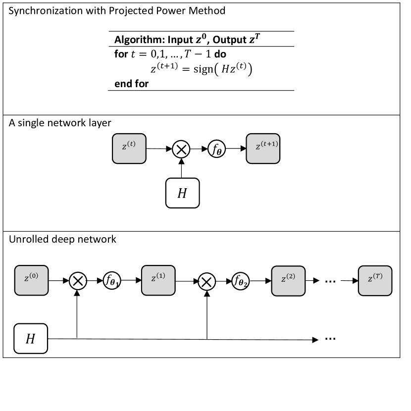
Figure 1: The concept of an unrolled algorithm for $\mathbb{Z}/2$ synchronization based on the projected power method. The upper panel shows the standard projected power method for $\mathbb{Z}/2$ synchronization with $T$ iterations; see Section II-A2. The middle panel illustrates a single iteration of the algorithm in the form of a single-layer network, where the sign operator is replaced by a general, learned non-linear function $f_{\theta}$. The bottom panel shows the concatenation of $T$ layers into an unrolled deep network. Each layer may have a separate set of parameters. The Onsager correction term that uses $z^{(t-1)}$ is omitted for simplicity.

III-A Architecture and loss function for $\mathbb{Z}/2$ synchronization

Following the AMP iterations in (II.6) and (II.7), the $(t+1)$-th layer receives as input the measurement matrix $H\in\mathbb{R}^{N\times N}$, and the previous layers’ estimates $z^{(t)},z^{(t-1)}\in\mathbb{R}^{N}$. The output $z^{(t+1)}\in\mathbb{R}^{N}$ can be described using the following equations:

$$c=\theta_{0}\lambda Hz^{(t)}-\lambda^{2}(1-\langle(\phi_{\boldsymbol{\theta}_{2}}(z^{(t)}))^{2}\rangle)z^{(t-1)},$$ (III.3)

and

$$z^{(t+1)}=f_{\boldsymbol{\theta}_{1}}\left(c\right),$$ (III.4)

where $f$ and $\phi$ are learned functions parameterized by a set of weights $\boldsymbol{\theta}_{1}$ and $\boldsymbol{\theta}_{2}$.

We denote by Dense(N) a linear layer with $N$ neurons, whose input is the previous layer’s output, BatchNorm() denotes a batch normalization layer, ReLU() is a relu layer, and tanh() is a hyperbolic tangent layer. The learned function has the following structure: Dense(32) $\to$ BatchNorm() $\to$ ReLU() $\to$ Dense(1) $\to$ BatchNorm() $\to$ tanh(), such that its outputs are in the range $[-1,1]$.

Given a batch of size $M$, with ground truth and predicted group elements $\{z_{m}\}_{m=1}^{M}$ and $\{\hat{z}_{m}\}_{m=1}^{M}$, respectively, we use the following loss function to optimize the weights:

$$\mathcal{L}(\Theta)=1-\frac{1}{NM}\sum_{m=1}^{M}{|z_{m}^{T}\hat{z}_{m}|},$$ (III.5)

where $\Theta=[{\boldsymbol{\theta}^{(0)}},...,{\boldsymbol{\theta}^{(T-1)}}]$ is the set of parameters of the network, and $\boldsymbol{\theta}^{(t)}=[\theta^{(t)}_{0},\boldsymbol{\theta}^{(t)}_{1},\boldsymbol{\theta}^{(t)}_{2}]$ is the set of parameters per layer. The loss function (III.5) measures the average alignment error, up to a sign, between the predicted and the ground truth group elements over $M$ samples. The absolute value function is required due to the sign symmetry.

III-B Architecture and loss function for $U(1)$ synchronization

Based on the AMP iterations (II.12) and (II.11), the $(t+1)$-th layer receives as input $H_{r},H_{i}\in\mathbb{R}^{N\times N}$, the real and imaginary parts of the measurement matrix, respectively, and $z^{(t)}_{r},z^{(t)}_{i},z^{(t-1)}_{r},z^{(t-1)}_{i}\in\mathbb{R}^{N}$: the real and imaginary parts of the estimates of the previous layers. The output $z^{(t+1)}_{r},z^{(t+1)}_{i}\in\mathbb{R}^{N}$ can be described using the following equations:

$$c_{r}=\theta_{0}\lambda(H_{r}z^{(t)}_{r}-H_{i}z^{(t)}_{i})-\lambda^{2}(1-\langle{z^{(t)}_{r}}^{2}+{z^{(t)}_{i}}^{2}\rangle)z^{(t-1)}_{r},$$

$$c_{i}=\theta_{0}\lambda(H_{r}z^{(t)}_{i}+H_{i}z^{(t)}_{r})-\lambda^{2}(1-\langle{z^{(t)}_{r}}^{2}+{z^{(t)}_{i}}^{2}\rangle)z^{(t-1)}_{i}$$ (III.6)

and

$$z^{(t+1)}_{r}[n]=\frac{c_{r}[j]}{\max\left(|c[j]|,\varepsilon\right)}f_{\boldsymbol{\theta}_{1}}\left(|c[j]|\right),$$

$$z^{(t+1)}_{i}[j]=\frac{c_{i}[j]}{\max\left(|c[j]|,\varepsilon\right)}f_{\boldsymbol{\theta}_{1}}\left(|c[j]|\right),$$ (III.7)

where $|c[j]|=\sqrt{{c_{r}[j]}^{2}+{c_{i}[j]}^{2}}$, and $\varepsilon=10^{-12}$ is a small constant that is introduced for numerical stability. The non-linear function $f$ is a learned function parameterized by a set of weights $\boldsymbol{\theta}_{1}$ with the following structure: Dense(256) $\to$ ReLU() $\to$ Dense(1) $\to$ tanh(), such that its outputs are within $[-1,1]$.

Let $\{z_{r_{m}}\}_{m=1}^{M},\{z_{i_{m}}\}_{m=1}^{M}$ and $\{\hat{z}_{r_{m}}\}_{m=1}^{M},\{\hat{z}_{i_{m}}\}_{m=1}^{M}$ be the real and imaginary parts of the ground truth and the predicted group elements, respectively, of a batch of size $M$. We use the following loss function to optimize the weights:

$$\begin{split}\mathcal{L}(\Theta)=1-\frac{1}{NM}\sum_{m=1}^{M}&\left[(z_{r_{m}}^{T}\hat{z}_{r_{m}}+z_{i_{m}}^{T}\hat{z}_{i_{m}})^{2}\right.\\ &\left.+(z_{r_{m}}^{T}\hat{z}_{i_{m}}-z_{i_{m}}^{T}\hat{z}_{r_{m}})^{2}\right]^{1/2},\end{split}$$ (III.8)

where $\Theta=[{\boldsymbol{\theta}^{(0)}},...,{\boldsymbol{\theta}^{(T-1)}}]$ is the set of network’s parameters, and $\boldsymbol{\theta}^{(t)}=[\theta^{(t)}_{0},\boldsymbol{\theta}^{(t)}_{1}]$. This loss function measures the alignment between the ground truth and predicted group elements, and it is invariant to a global phase shift (the symmetry of the problem).

III-C Architecture and loss function for $SO(3)$ synchronization

The projection operation in equation (II.16), which consists of SVD factorization, is non-differentiable and thus gradients cannot be back-propagated through it during the learning process. Therefore, in order to unroll the projected power method into a differentiable neural network, this projection operation should be replaced. To derive a differentiable projection operation, we start with an alternative method that expresses the nearest orthogonal matrix of a matrix $A$, denoted by $Q$, explicitly using the matrix square root: $Q=A(A^{T}A)^{-\frac{1}{2}}$. This method can be combined with the Babylonian method, and a first order approximation suggests the following iterations after setting $Q_{0}=A/\|A\|_{\text{F}}$ [15]:

$$N_{i}=Q_{i}^{T}Q_{i}$$ (III.9)

$$P_{i}=\frac{1}{2}Q_{i}N_{i}$$

$$Q_{i+1}=2Q_{i}+P_{i}N_{i}-3P_{i}.$$

Numerical experiments suggest that this recursion typically converges after 4 iterations. We thus use $Q_{4}$ as an estimation for the nearest orthogonal matrix of $A$, through which gradients can be backpropagated.

The unrolled synchronization algorithm for $SO(3)$ is composed of a stacked learned synchronization blocks, followed by a projection block as the last layer. Each learned synchronization block takes on the form:

$$R^{(t+1)}=f_{\boldsymbol{\theta}_{1}}(HR^{(t)})+\phi_{\boldsymbol{\theta}_{2}}(R^{(t-1)}).$$ (III.10)

The function implementation consists of the following layers: Reshape input $(M,3N,3)$ to $(M,N,9)$ $\to$ Dense(hidden neurons) $\to$ BatchNorm() $\to$ ReLU() $\to$ Dense(9) $\to$ BatchNorm() $\to$ tanh() $\to$ Reshape into $(M,3N,3)$, where $M$ is the batch size. The first layer reshapes the input such that each $3\times 3$ block is flattened into 9 elements, resulting in a shape of $(M,N,9)$. The following layers apply the same non-linear functions to each 9-element vector and reshape them back into the dimensions of the input. The function $f$ uses 32 hidden neurons and $\phi$ uses 9 hidden neurons. The function $\phi$ acts as the Onsager correction term and slightly improves the results.

The implementation of the projection block is as follows:

1. reshape input $(M,3N,3)$ to $(M,N,3,3)$;

2. normalize each $3\times 3$ matrix by its Frobenius norm and apply the four iterations of (III.9);

3. reshape the output of the last stage to $(M,3N,3)$.

Given a batch of samples of size $M$, with ground truth and predicted group elements $\{R_{m}\}_{m=1}^{M}$ and $\{\hat{R}_{m}\}_{m=1}^{M}$, respectively, we use the following loss function to optimize the weights:

$$\mathcal{L}(\Theta)=1-\frac{3}{NM}\sum_{m=1}^{M}{\|R_{m}^{T}\hat{R}_{m}\|_{\text{F}}^{2}},$$ (III.11)

where $\Theta=[{\boldsymbol{\theta}^{(0)}},...,{\boldsymbol{\theta}^{(T-1)}}]$ is the set of network’s parameters, and $\boldsymbol{\theta}^{(t)}=[\boldsymbol{\theta}^{(t)}_{1},\boldsymbol{\theta}^{(t)}_{2}]$. The suggested loss measures the alignment between the ground truth and the predicted group element matrices, and is invariant under a global rotation.

III-D Multi-reference alignment (MRA)

MRA models differ from group synchronization in two important aspects. First, the goal of the MRA problem is not to estimate the group elements, but the signal itself. Second, the pairwise ratios are not directly available, and are estimated from the observations. Therefore, the learning phase of MRA models is slightly different from group synchronization, as described below. We draw $M$ signals from some distribution. Then, for each signal, we generate $N$ noisy measurements according to the MRA statistical model, and estimate the pairwise ratio between the corresponding group elements. Given the pairwise ratio matrix, we solve a group synchronization problem and aim to estimate the signal itself, up to a group action. As we will see below, this process suggests different loss functions than the ones used for group synchronization.

III-D1 MRA over $\mathbb{Z}/2$

A direct application of the $\mathbb{Z}/2$ architecture described in Section III-A, when the pairwise ratios are estimated from the noisy measurements, only leads to a small improvement, as will be presented in Section IV. Therefore, we suggest to incorporate the measurements themselves in the loss function of the neural network.

Let $Y_{m}\in\mathbb{R}^{L\times N}$ be the measurement matrix of the $m$-th signal $x_{m}\in\mathbb{R}^{L}$, so that $Y_{m}[:,n]\in\mathbb{R}^{L}$ is the $n$-th observation of the $m$-th signal. We suggest the following reconstruction loss:

$$\mathcal{L}_{R}(\Theta)=\frac{1}{LM}\sum_{m=1}^{M}{\min_{s\in\{-1,1\}}\left\|x_{m}-\frac{s}{N}\sum_{n=1}^{N}{Y_{m}[:,n]\hat{z}_{m}[n]}\right\|^{2}},$$ (III.12)

where $\hat{z}_{m}\in\mathbb{R}^{N}$ is the predicted group elements output of the network described in Section III-A. The loss function depends on the parameters $\Theta$ through the group elements $\{\hat{z}_{m}[n]\}_{n,m=1}^{N,M}$. Note that the reconstruction loss is invariant to the inherent sign symmetry.

III-D2 MRA over the group $\mathbb{Z}/L$ of circular shifts

Similarly to the MRA model described above, when the relative shifts were estimated from the MRA measurements, only a minor improvement in signal estimation was achieved using the architecture of $U(1)$ synchronization from Section III-B. Thus, we aim to work with the measurements directly.

It is more convenient to express the loss function in Fourier domain, where a circular shift is mapped to a complex exponential. Let $\mathcal{X}_{m}\in\mathbb{C}^{L}$ be the Fourier transform of the $m$-th signal, and let $\mathcal{Y}_{m}\in\mathbb{C}^{L\times N}$ be the corresponding measurement matrix, where $\mathcal{{Y}}_{m}[:,n]$ is the Fourier transform of the $n$-th measurement of the $m$-th signal. Let $\mathcal{Y}_{r_{m}}$ and $\mathcal{Y}_{i_{m}}$ denote the real and imaginary parts of $\mathcal{Y}_{m}$, and let $\hat{z}_{m}\in U(1)$ be the estimated rotation using the synchronization algorithm described in Section III-B. Note that $\hat{z}_{m}$ lies on the unit circle, whereas the circular shifts are discrete. The real and imaginary parts of the aligned data matrix of the $m$-th sample can be written as:

$$\mathcal{\tilde{Y}}_{r_{m}}[k,n] =\cos\left(k\angle{\hat{z}_{m}}\right)\mathcal{Y}_{r_{m}}[k,n]-\sin\left(k\angle{\hat{z}_{m}}\right)\mathcal{Y}_{i_{m}}[k,n]$$

$$\mathcal{\tilde{Y}}_{i_{m}}[k,n] =\cos\left(k\angle{\hat{z}_{m}}^{T}\right)\mathcal{Y}_{i_{m}}[k,n]+\sin\left(k\angle{\hat{z}_{m}}^{T}\right)\mathcal{Y}_{r_{m}}[k,n],$$ (III.13)

for $k=0,...,L-1$. The signal is then estimated by averaging:

$$\hat{\mathcal{X}}_{m}=\frac{1}{N}\sum_{n=1}^{N}{\left(\mathcal{\tilde{Y}}_{r_{m}}[:,n]+\iota\mathcal{\tilde{Y}}_{i_{m}}[:,n]\right)}.$$ (III.14)

Therefore, we use the following loss function:

$$\mathcal{L}_{R}(\Theta)=c\sum_{m=1}^{M}{\min_{\phi\in\Phi_{P}}\sum_{k}\left(\mathcal{X}_{m}[k]-e^{jk\phi}\mathcal{\hat{X}}_{m}[k]\right)^{2},}$$ (III.15)

where $c=\frac{1}{L^{2}M}$ and $\Phi_{P}=\{\frac{2\pi}{LP},2\frac{2\pi}{LP},\ldots,2\pi\}$. In the numerical experiments below, we set $P=10$.

IV Numerical experiments

The following experiments examine the average error of the unrolled algorithms and the iterative algorithms described in Section II. In all experiments, we set $N=20$, and the number of test samples is equal to the number of training samples. The code to reproduce all experiments is publicly available at https://github.com/noamjanco/unrolling_synchronization.

IV-A $\mathbb{Z}/2$ synchronization

For a vector of ground truth group elements $z\in\{\pm 1\}^{N}$ and a prediction $\hat{z}$, the alignment error is defined as:

$$\text{error}(z,\hat{z})=1-\frac{|z^{T}\hat{z}|}{N}.$$ (IV.1)

We note that $\text{error}(z,\hat{z})=0$ for an ideal estimation, where $\hat{z}=\pm z$. In addition, the error is invariant to a global sign, i.e., $\text{error}(z,-\hat{z})=\text{error}(z,\hat{z})$.

Each observation of length $N=20$ was generated according to  (II.1), where each entry was drawn i.i.d. from a uniform distribution over $\pm 1$. The network was trained using a dataset of size $M=20000$, with $300$ epochs, and a learning rate of $10^{-3}$, using the Adam optimizer with batch size of $128$.

The alignment error as a function of depth is presented in Figure 2, for SNR values of $\lambda=1.2$, $\lambda=1.5$ and $\lambda=2$. We compared the performance of the unrolled algorithm against the alternative algorithms described in Section II-A, where the number of iterations is equal to the depth of the network. The results demonstrate that the unrolled synchronization network achieves better error performance, and the performance gap increases as the SNR decreases.

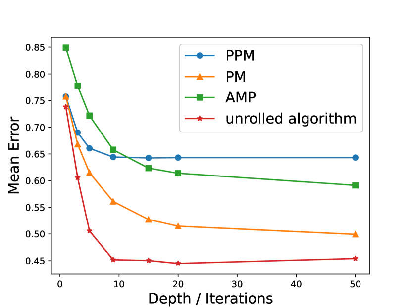
(a) $\lambda=1.2$

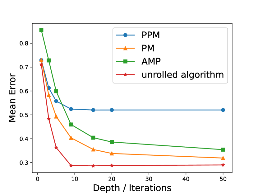
(b) $\lambda=1.5$

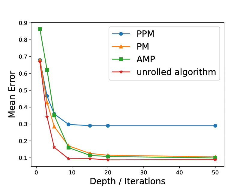
(c) $\lambda=2$

Figure 2: Alignment error (IV.1) as a function of depth for the $\mathbb{Z}/2$ synchronization problem with different $\lambda$ values. The unrolled algorithm is compared against the power method (PM), projected power method (PPM), and the AMP algorithm described in Section II-A. The unrolled synchronization network outperforms the alternative algorithms, and the gap increases as the SNR decreases.

Figure 3 shows the alignment error as a function of SNR, with a network of a fixed depth of 9, while the alternative algorithms used 100 iterations. We see that the neural network outperforms the alternative methods in terms of alignment error with much fewer iterations.

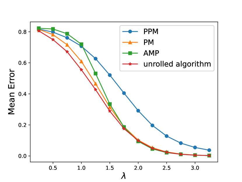
Figure 3: Alignment error (IV.1) as a function of the SNR for $\mathbb{Z}/2$ synchronization. The depth of the unrolled algorithm is fixed to 9, while the alternative algorithms ran for 100 iterations. Nevertheless, the unrolled algorithm clearly outperforms the iterative methods.

IV-B $U(1)$ synchronization

We define the error between the vector of the ground truth group elements $z\in\mathbb{C}_{1}^{N}$ and a prediction $\hat{z}\in\mathbb{C}_{1}^{N}$ by:

$$\text{error}(z,\hat{z})=1-\frac{|z^{*}\hat{z}|}{N}.$$ (IV.2)

We note that $\text{error}(z,\hat{z})=0$ when $\hat{z}=ze^{\iota\phi}$ for any $\phi\in[0,2\pi)$. Generally, the error is invariant to a global phase since $\text{error}(z,e^{\iota\phi}\hat{z})=\text{error}(z,\hat{z})$ for any $\phi\in[0,2\pi)$.

The network was trained using a data set of dimension $N=20$ and $M=20000$ samples generated according to the model in (II.8). We used the Adam optimizer with batch size of $128$, $300$ epochs, and a learning rate of $10^{-4}$. The results are presented in Figure 4 for $\lambda=1.2$, $\lambda=1.5$ and $\lambda=2$. As in the $\mathbb{Z}/2$ synchronization, the unrolled synchronization network outperforms the alternative algorithms, especially as the SNR decreases.

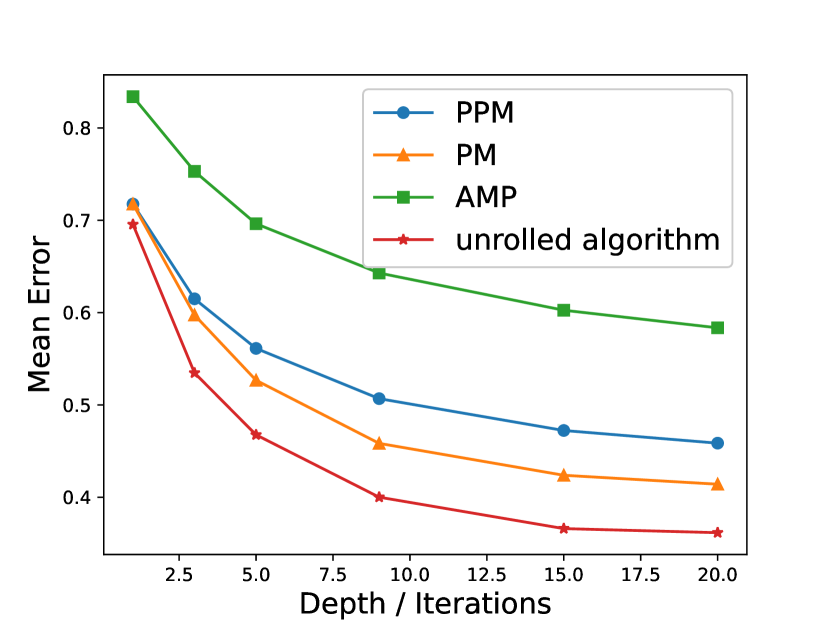
(a) $\lambda=1.2$

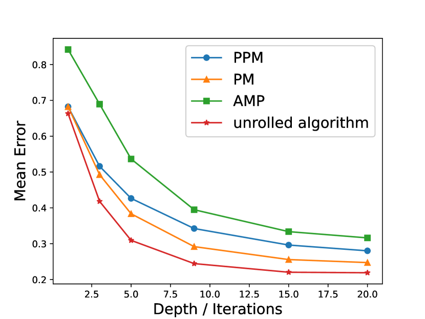
(b) $\lambda=1.5$

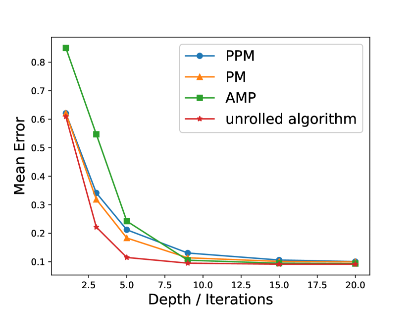
(c) $\lambda=2$

Figure 4: Alignment error (IV.2) as a function of depth for the $U(1)$ synchronization problem with different $\lambda$ values. The unrolled algorithm is compared against the power method (PM), projected power method (PPM), and the AMP algorithm described in Section II-B.

IV-C $SO(3)$ synchronization

For a ground truth matrix $R\in\mathbb{R}^{3N\times 3}$ (composed of $N,3\times 3$ rotation matrices) and a prediction $\hat{R}\in\mathbb{R}^{3N\times 3}$, the error is defined as:

$$\text{error}(R,\hat{R})=1-\frac{3}{N}\left\|R^{T}\hat{R}\right\|_{\text{F}}^{2}.$$ (IV.3)

This error metric is invariant to a right multiplication by an orthogonal matrix, and is equal to zero if $\hat{R}$ is equal to $R$ (up to a global rotation).

The network was trained using a dataset of dimension $N=20$ and $M=10000$ samples generated according to the model in (II.14). We used the Adam optimizer with batch size of $128$, $300$ epochs, and a learning rate of $10^{-2}$. The spectral method computed the first three eigenvectors of the measurement matrix using SVD factorization as described in II-C1. Therefore, its error is not a function of the number of iterations. The results are presented in Figure 5, demonstrating a substantial gap between the unrolled algorithm and the competitors.

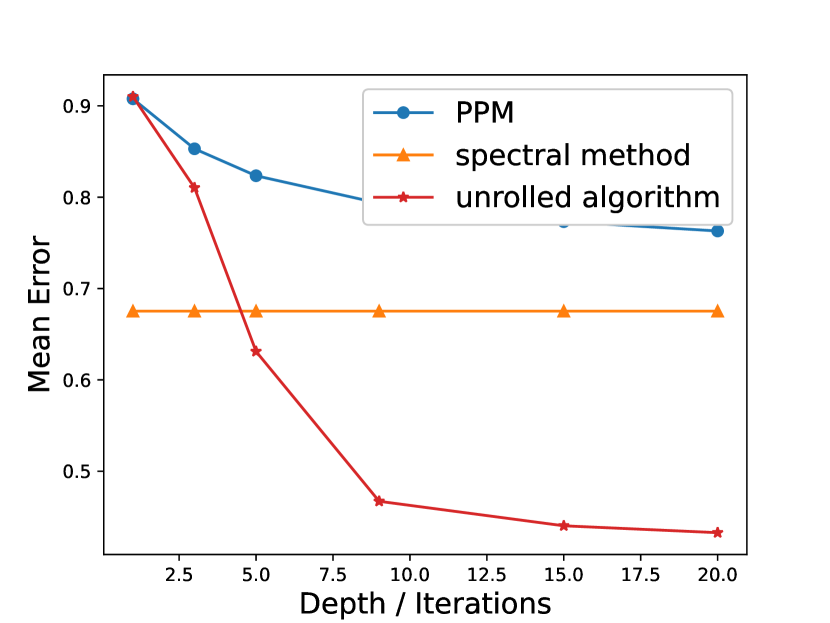
(a) $\lambda=1.2$

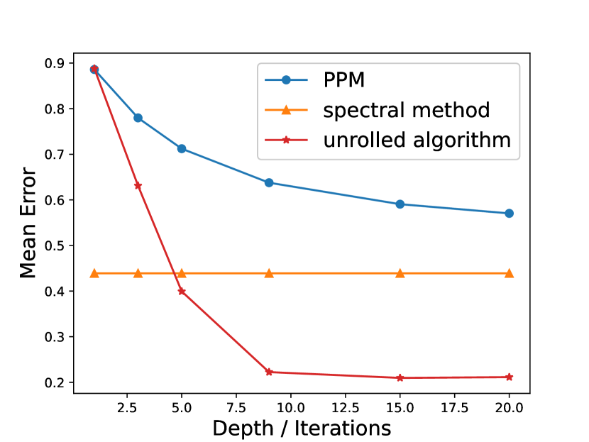
(b) $\lambda=1.5$

(c) $\lambda=2$

Figure 5: Alignment error (IV.3) as a function of depth for the $SO(3)$ synchronization problem with different $\lambda$ values. The unrolled algorithm is compared against the spectral method and the projected power method (PPM) as described in Section II-C. We note that the spectral method computes the eigenvectors using SVD factorization, and thus the error is not a function of the number of iterations.

Figure 6 shows the error as a function of the SNR, when the depth of the network was fixed to 9, while the projected power method ran for 100 iterations. Nevertheless, the unrolled algorithm clearly outperforms the other methods.

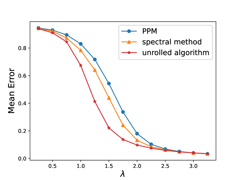
Figure 6: Alignment error (IV.3) as a function of the SNR for $SO(3)$ synchronization. The depth of the unrolled algorithm is fixed to 9, while the alternative algorithms ran for 100 iterations. Nevertheless, the unrolled algorithm clearly outperforms the iterative methods.

In addition, we measured the inference run-time of a batch of 10000 samples with $\lambda=1.5$, $N=20$ and $L=9$ layers, and compared it against PPM with 100 iterations and the spectral method. The results are summarized in Table I. The unrolled algorithm outperforms both methods in terms of alignment error and total run-time due to its low number of layers, with only a slight increase in run-time per layer.

Algorithm	Alignment Error	Total run-time [sec]	Single iteration run-time [sec]
Spectral method	0.439003	18.96	-
Projected power method	0.637658	37.52	0.375
Unrolled synchronization	0.221980	3.53	0.392

TABLE I: Run-time for SO(3) synchronization with a batch of 10000 samples, $\lambda=1.5$, $N=20$ and $L=9$ layers, compared against PPM with 100 iterations and the spectral method.

IV-D Multi-reference alignment over $\mathbb{Z}/2$

We generated measurements according to (II.17) with a signal length of 21, where each entry was drawn i.i.d. from $\mathcal{N}(0,1)$, and $N=20$. The relative ratios were estimated according to (II.18). In the first part, we evaluate the alignment error (IV.1) using the network described in III-A. In the next part, we evaluate the reconstruction error, defined as:

$$\text{error}(x,\hat{x})=\min_{s\in\{-1,1\}}\left\|x-s\hat{x}\right\|^{2},$$ (IV.4)

where $\hat{x}$ is the estimated signal, computed by aligning the measurements according to the estimated group elements and averaging, as described in (II.19). In this case, we used a modified loss function as described in III-D1.

IV-D1 With alignment loss (III.5)

The network was trained using a dataset of $M=10000$ samples, a batch size of $128$, with $300$ epochs, and a learning rate of $10^{-4}$, using the Adam optimizer. The average alignment error as a function of depth is presented in Figure 7, for $\lambda=0.2$ and $\lambda=0.3$. The experiment shows that the unrolled synchronization network usually achieves better error performance but the gap is insignificant.

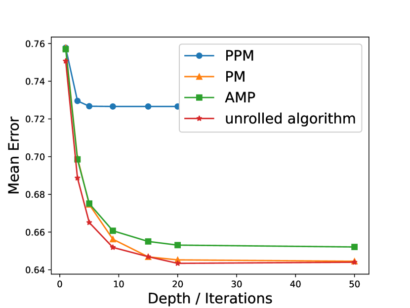
(a) $\lambda=0.2$

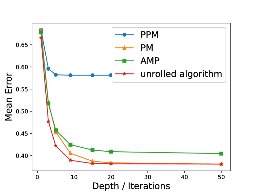
(b) $\lambda=0.3$

Figure 7: Alignment error (IV.1) as a function of depth for the multi-reference alignment over $\mathbb{Z}/2$ problem with different $\lambda$ values. The unrolled algorithm is compared against the power method (PM), projected power method (PPM), and the AMP algorithm described in Section II-D1.

IV-D2 With reconstruction loss (III.12)

The network was trained using a dataset of $M=10000$ samples, a batch size of $128$, with $300$ epochs, and a learning rate of $10^{-3}$, using the Adam optimizer. The average reconstruction error as a function of depth is presented in Figure 8 for $\lambda=0.4$ and $\lambda=0.8$. The experiment shows that the unrolled synchronization network achieves better reconstruction error performance per depth, and outperforms the existing methods for large number of iterations.

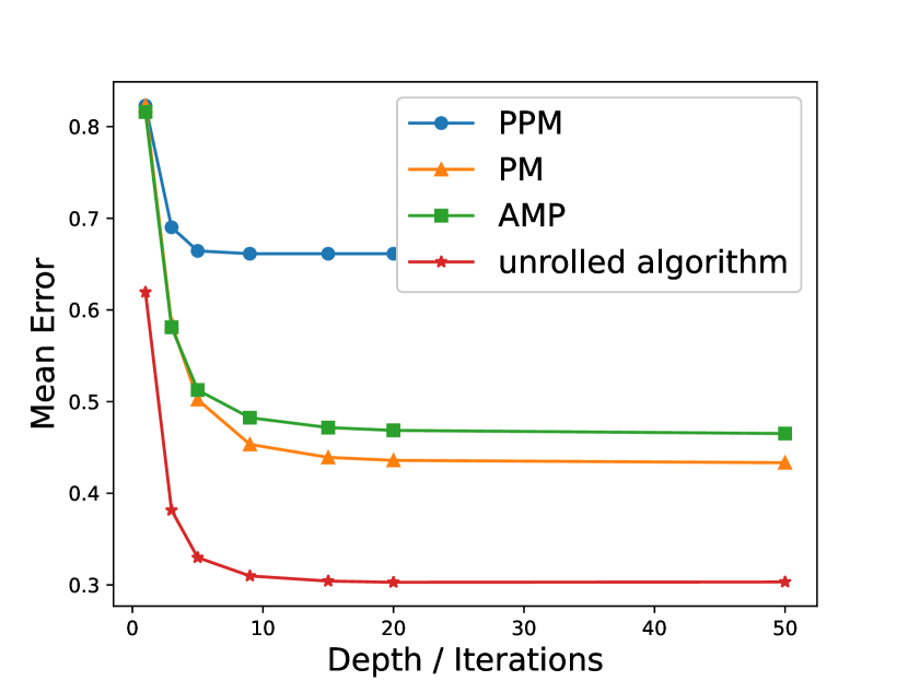
(a) $\lambda=0.4$

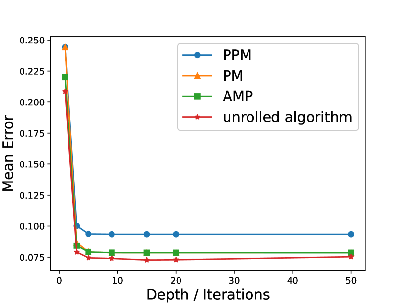
(b) $\lambda=0.8$

Figure 8: Reconstruction error (IV.4) as a function of depth for the multi-reference alignment over $\mathbb{Z}/2$ problem with different $\lambda$ values. The unrolled algorithm, trained using the reconstruction loss function described in Section III-D1, is compared against the power method (PM), projected power method (PPM), and the AMP algorithm described in Section II-D1.

IV-E Multi-reference alignment over the group $\mathbb{Z}/L$ of circular shifts

We generated measurements according to (II.21) with a signal of length 21, where each element was drawn i.i.d. from $\mathcal{N}(0,1)$, and $N=20$. The relative ratios were estimated according to (II.22) and (II.23). In the first part, we evaluate the alignment error (IV.2) using the network described in III-B. In the next part, we evaluate the signal reconstruction error, defined as:

$$\text{error}(\mathcal{X},\hat{\mathcal{X}})=\min_{\phi\in\{\frac{2\pi}{LP},2\frac{2\pi}{LP}...,2\pi\}}\|\mathcal{X}-e^{j\bar{k}\phi}\cdot\hat{\mathcal{X}}\|^{2},$$ (IV.5)

where $\bar{k}$ is the frequency vector at each entry, $\cdot$ is an entrywise product, and $\hat{\mathcal{X}}$ is the estimated signal in Fourier space, computed by aligning the measurements according to the estimated group elements and averaging, as described in (III-D2) and (III.14). In this case, we used a modified loss function as described in III-D2. We set $P=10$.

IV-E1 With alignment loss (III.8)

The network was trained using a dataset of $M=10000$ samples, a batch size of $128$, with $300$ epochs, and a learning rate of $10^{-4}$, using the Adam optimizer. The average alignment error as a function of depth is presented in Figure 9 for $\lambda=0.7$. The experiment shows that the error of the unrolled synchronization network improves with the depth of the network, but does not outperform the existing methods for large number of iterations.

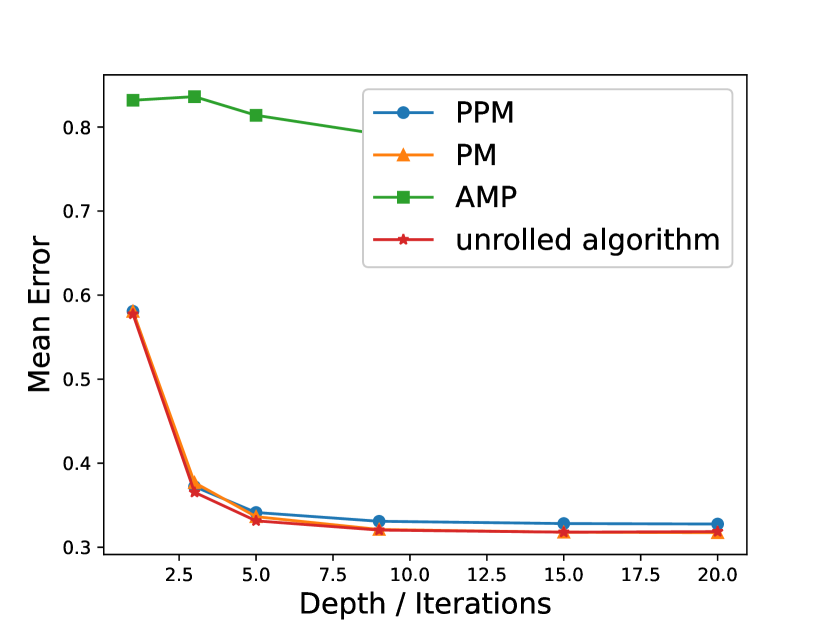
Figure 9: Alignment error (IV.1) as a function of depth for the multi-reference alignment over $\mathbb{Z}/L$ with $\lambda=0.7$. The unrolled algorithm is compared against the power method (PM), projected power method (PPM), and the AMP algorithm described in Section II-D2.

IV-E2 With reconstruction loss (III.15)

The network was trained using a dataset of $M=10000$ samples, a batch size of $128$, with $300$ epochs, and a learning rate of $10^{-1}$, using the Adam optimizer. The average alignment error as a function of depth is presented in Figure 10 for $\lambda=1$. The experiment shows that the unrolled synchronization network clearly outperforms the existing methods for large number of iterations.

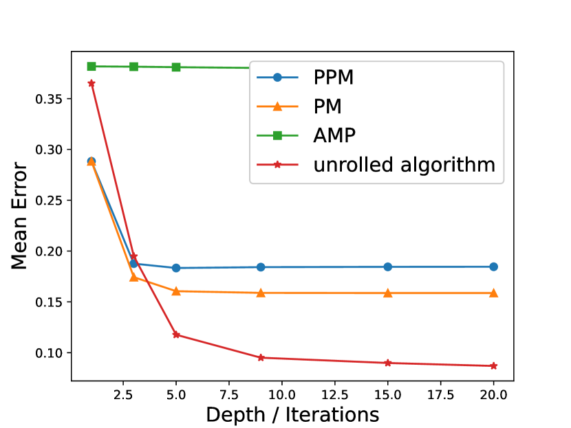
Figure 10: Reconstruction error (IV.5) as a function of depth for the multi-reference alignment over $\mathbb{Z}/L$ problem with $\lambda=1$. The unrolled algorithm, trained using the reconstruction loss function described in Section III-D2, is compared against the power method (PM), projected power method (PPM), and the AMP algorithm described in Section II-D2.

V Discussion

In this paper, we have presented a new computational framework for the group synchronization problem, based on unrolling existing synchronization algorithms, and optimize them using training data. We introduced unrolling strategies to a wide variety of group synchronization problems, trained using a differentiable invariant synchronization loss function that measures the alignment of the ground truth and the predicted group elements. We have shown that the designed algorithms outperform existing methods for group synchronization. For SO(3) synchronization, we suggested a differentiable feed-forward approximation for the projection operation which enables training the unrolled algorithm. For the MRA problem, the proposed algorithm incorporates signal prior into the unrolling synchronization algorithm, since the training data consists of relative rotations estimated from noisy measurements drawn according to the signal prior.

In the $\mathbb{Z}/2$ synchronization problem, we have demonstrated how the suggested method achieves lower alignment error in the low and moderate SNR regimes, with fewer iterations. In the high SNR regime the performance of all algorithms is comparable, but the unrolled algorithm still achieves a smaller error per iteration. We then conclude that the proposed method is beneficial for lower SNR regimes, and when running-time is a major concern. While existing methods such as AMP have asymptotic error guarantees, our experiments demonstrate that for a fixed and small number of samples the unrolled synchronization is favorable. We believe that the improved performance stems from our general strategy to optimize existing algorithms (such as AMP) using training data. Moreover, the unrolling synchronization can be readily applied to other noise models, beyond the Gaussian model.

An interesting question is to examine whether a similar technique can be designed for the non-unique games problem: a general optimization framework over groups that can be interpreted as a generalization of the group synchronization problem [8].

The recent interest in the group synchronization and MRA problems, and this paper in specific, is mainly motivated by the cryo-EM technology to reconstruct 3-D molecular structures [10]. In cryo-EM, each observation is a noisy tomographic projection of the molecular structure, taken from some unknown viewing direction. In particular, under some simplifying assumptions, the $i$-th cryo-EM observation is modeled as

$$I_{i}=PR_{\omega_{i}}\phi+\varepsilon_{i},$$ (V.1)

where $\phi:\mathbb{R}^{3}\to\mathbb{R}$ is the sought 3-D structure, $R_{\omega}$ is a 3-D rotation by $\omega\in\text{SO}(3)$, P is a fixed tomographic projection, and $\varepsilon$ is an additive noise. The goal is to estimate $\phi$, from $I_{1},\ldots,I_{N},$ while the rotations $R_{1},\ldots,R_{N}\in SO(3)$ are unknown.

One approach to solve the cryo-EM problem is to estimate the missing rotations from the observations and then recover the 3-D structure as a linear problem. This methodology is used to constitute ab initio models [24]. In [46, 47, 45, 43], it was shown that the pairwise relative rotations $\{R_{\omega_{i}}R_{\omega_{j}}^{-1}\}_{i,j=1}^{N}$ can be estimated from the observations based on the common lines property. Therefore, the cryo-EM reconstruction problem boils down to a synchronization problem over SO(3). Our ultimate goal is to apply our unrolled SO(3) algorithm to cryo-EM experimental data sets. To train the network, in addition to simulated data as in this paper, we intend to use experimental data of previously resolved structures available in public repositories [26], and structures resolved using computational tools such as AlphaFold [29].

Another possible future research thread is replacing the unrolling strategy with deep equilibrium (DEQ) to enable a forward model corresponding to an infinite number of layers [4]. Although DEQ models were developed for sequence modeling, it may fit the group synchronization problem: the input sequence is analog to the relative measurement matrix $H$ that is shared among the layers, and the hidden sequence is analog to the estimated group elements.

References

- [1] Asaf Abas, Tamir Bendory, and Nir Sharon. The generalized method of moments for multi-reference alignment. IEEE Transactions on Signal Processing, 70:1377–1388, 2022.
- [2] Emmanuel Abbe. Community detection and stochastic block models: recent developments. The Journal of Machine Learning Research, 18(1):6446–6531, 2017.
- [3] Emmanuel Abbe, Tamir Bendory, William Leeb, João M Pereira, Nir Sharon, and Amit Singer. Multireference alignment is easier with an aperiodic translation distribution. IEEE Transactions on Information Theory, 65(6):3565–3584, 2018.
- [4] Shaojie Bai, J. Zico Kolter, and Vladlen Koltun. Deep equilibrium models. 2019.
- [5] Afonso S Bandeira, Ben Blum-Smith, Joe Kileel, Amelia Perry, Jonathan Weed, and Alexander S Wein. Estimation under group actions: recovering orbits from invariants. arXiv preprint arXiv:1712.10163, 2017.
- [6] Afonso S Bandeira, Nicolas Boumal, and Amit Singer. Tightness of the maximum likelihood semidefinite relaxation for angular synchronization. Mathematical Programming, 163(1):145–167, 2017.
- [7] Afonso S Bandeira, Moses Charikar, Amit Singer, and Andy Zhu. Multireference alignment using semidefinite programming. In Proceedings of the 5th conference on Innovations in theoretical computer science, pages 459–470, 2014.
- [8] Afonso S Bandeira, Yutong Chen, Roy R Lederman, and Amit Singer. Non-unique games over compact groups and orientation estimation in cryo-EM. Inverse Problems, 36(6):064002, 2020.
- [9] Afonso S Bandeira, Jonathan Niles-Weed, and Philippe Rigollet. Optimal rates of estimation for multi-reference alignment. Mathematical Statistics and Learning, 2(1):25–75, 2020.
- [10] Tamir Bendory, Alberto Bartesaghi, and Amit Singer. Single-particle cryo-electron microscopy: Mathematical theory, computational challenges, and opportunities. IEEE Signal Processing Magazine, 37(2):58–76, 2020.
- [11] Tamir Bendory, Nicolas Boumal, Chao Ma, Zhizhen Zhao, and Amit Singer. Bispectrum inversion with application to multireference alignment. IEEE Transactions on Signal Processing, 66(4):1037–1050, 2017.
- [12] Tamir Bendory, Dan Edidin, William Leeb, and Nir Sharon. Dihedral multi-reference alignment. IEEE Transactions on Information Theory, 68(5):3489–3499, 2022.
- [13] Tamir Bendory, Yonina C Eldar, and Nicolas Boumal. Non-convex phase retrieval from STFT measurements. IEEE Transactions on Information Theory, 64(1):467–484, 2017.
- [14] Tamir Bendory, Ido Hadi, and Nir Sharon. Compactification of the rigid motions group in image processing. SIAM Journal on Imaging Sciences, 15(3):1041–1078, 2022.
- [15] Å. Björck and C. Bowie. An iterative algorithm for computing the best estimate of an orthogonal matrix. SIAM Journal on Numerical Analysis, 8(2):358–364, 1971.
- [16] Nicolas Boumal. Nonconvex phase synchronization. SIAM Journal on Optimization, 26(4):2355–2377, 2016.
- [17] Nicolas Boumal, Tamir Bendory, Roy R Lederman, and Amit Singer. Heterogeneous multireference alignment: A single pass approach. In 2018 52nd Annual Conference on Information Sciences and Systems (CISS), pages 1–6. IEEE, 2018.
- [18] Jesus Briales and Javier Gonzalez-Jimenez. Cartan-sync: Fast and global SE (d)-synchronization. IEEE Robotics and Automation Letters, 2(4):2127–2134, 2017.
- [19] Siheng Chen, Yonina C Eldar, and Lingxiao Zhao. Graph unrolling networks: Interpretable neural networks for graph signal denoising. IEEE Transactions on Signal Processing, 69:3699–3713, 2021.
- [20] Yunjin Chen and Thomas Pock. Trainable nonlinear reaction diffusion: A flexible framework for fast and effective image restoration. IEEE transactions on pattern analysis and machine intelligence, 39(6):1256–1272, 2016.
- [21] Il Yong Chun, Zhengyu Huang, Hongki Lim, and Jeff Fessler. Momentum-net: Fast and convergent iterative neural network for inverse problems. IEEE Transactions on Pattern Analysis and Machine Intelligence, pages 1–1, 2020.
- [22] Mihai Cucuringu. Sync-rank: Robust ranking, constrained ranking and rank aggregation via eigenvector and SDP synchronization. IEEE Transactions on Network Science and Engineering, 3(1):58–79, 2016.
- [23] Mihai Cucuringu, Yaron Lipman, and Amit Singer. Sensor network localization by eigenvector synchronization over the euclidean group. ACM Transactions on Sensor Networks (TOSN), 8(3):1–42, 2012.
- [24] Ido Greenberg and Yoel Shkolnisky. Common lines modeling for reference free ab-initio reconstruction in cryo-EM. Journal of structural biology, 200(2):106–117, 2017.
- [25] Karol Gregor and Yann LeCun. Learning fast approximations of sparse coding. In Proceedings of the 27th international conference on international conference on machine learning, pages 399–406, 2010.
- [26] Andrii Iudin, Paul K Korir, José Salavert-Torres, Gerard J Kleywegt, and Ardan Patwardhan. EMPIAR: a public archive for raw electron microscopy image data. Nature methods, 13(5):387–388, 2016.
- [27] Mark A Iwen, Aditya Viswanathan, and Yang Wang. Fast phase retrieval from local correlation measurements. SIAM Journal on Imaging Sciences, 9(4):1655–1688, 2016.
- [28] Noam Janco and Tamir Bendory. An accelerated expectation-maximization algorithm for multi-reference alignment. IEEE Transactions on Signal Processing, 70:3237–3248, 2022.
- [29] John Jumper, Richard Evans, Alexander Pritzel, Tim Green, Michael Figurnov, Olaf Ronneberger, Kathryn Tunyasuvunakool, Russ Bates, Augustin Žídek, Anna Potapenko, et al. Highly accurate protein structure prediction with AlphaFold. Nature, 596(7873):583–589, 2021.
- [30] Yuelong Li, Mohammad Tofighi, Vishal Monga, and Yonina C Eldar. An algorithm unrolling approach to deep image deblurring. In ICASSP 2019-2019 IEEE International Conference on Acoustics, Speech and Signal Processing (ICASSP), pages 7675–7679. IEEE, 2019.
- [31] Shuyang Ling. Near-optimal performance bounds for orthogonal and permutation group synchronization via spectral methods. Applied and Computational Harmonic Analysis, 60:20–52, 2022.
- [32] Chao Ma, Tamir Bendory, Nicolas Boumal, Fred Sigworth, and Amit Singer. Heterogeneous multireference alignment for images with application to 2D classification in single particle reconstruction. IEEE Transactions on Image Processing, 29:1699–1710, 2019.
- [33] Stefano Marchesini, Yu-Chao Tu, and Hau-tieng Wu. Alternating projection, ptychographic imaging and phase synchronization. Applied and Computational Harmonic Analysis, 41(3):815–851, 2016.
- [34] Abolfazl Mehranian and Andrew J. Reader. Model-based deep learning pet image reconstruction using forward–backward splitting expectation–maximization. IEEE Transactions on Radiation and Plasma Medical Sciences, 5(1):54–64, 2021.
- [35] Vishal Monga, Yuelong Li, and Yonina C Eldar. Algorithm unrolling: Interpretable, efficient deep learning for signal and image processing. IEEE Signal Processing Magazine, 38(2):18–44, 2021.
- [36] Onur Ozyesil, Nir Sharon, and Amit Singer. Synchronization over Cartan motion groups via contraction. SIAM Journal on Applied Algebra and Geometry, 2(2):207–241, 2018.
- [37] Onur Özyeşil, Vladislav Voroninski, Ronen Basri, and Amit Singer. A survey of structure from motion. Acta Numerica, 26:305–364, 2017.
- [38] Amelia Perry, Jonathan Weed, Afonso S Bandeira, Philippe Rigollet, and Amit Singer. The sample complexity of multireference alignment. SIAM Journal on Mathematics of Data Science, 1(3):497–517, 2019.
- [39] Amelia Perry, Alexander S Wein, Afonso S Bandeira, and Ankur Moitra. Message-passing algorithms for synchronization problems over compact groups. Communications on Pure and Applied Mathematics, 71(11):2275–2322, 2018.
- [40] Elad Romanov, Tamir Bendory, and Or Ordentlich. Multi-reference alignment in high dimensions: sample complexity and phase transition. SIAM Journal on Mathematics of Data Science, 3(2):494–523, 2021.
- [41] David M Rosen, Luca Carlone, Afonso S Bandeira, and John J Leonard. SE-Sync: A certifiably correct algorithm for synchronization over the special Euclidean group. The International Journal of Robotics Research, 38(2-3):95–125, 2019.
- [42] Yair Ben Sahel, John P Bryan, Brian Cleary, Samouil L Farhi, and Yonina C Eldar. Deep unrolled recovery in sparse biological imaging: Achieving fast, accurate results. IEEE Signal Processing Magazine, 39(2):45–57, 2022.
- [43] Yoel Shkolnisky and Amit Singer. Viewing direction estimation in cryo-EM using synchronization. SIAM journal on imaging sciences, 5(3):1088–1110, 2012.
- [44] Amit Singer. Angular synchronization by eigenvectors and semidefinite programming. Applied and computational harmonic analysis, 30(1):20–36, 2011.
- [45] Amit Singer and Yoel Shkolnisky. Three-dimensional structure determination from common lines in cryo-EM by eigenvectors and semidefinite programming. SIAM journal on imaging sciences, 4(2):543–572, 2011.
- [46] BK Vainshtein and AB Goncharov. Determination of the spatial orientation of arbitrarily arranged identical particles of unknown structure from their projections. In Soviet Physics Doklady, volume 31, page 278, 1986.
- [47] Marin Van Heel. Angular reconstitution: a posteriori assignment of projection directions for 3D reconstruction. Ultramicroscopy, 21(2):111–123, 1987.
- [48] Dufan Wu, Kyungsang Kim, and Quanzheng Li. Computationally efficient deep neural network for computed tomography image reconstruction. Med. Phys., 46(11):4763–4776, November 2019.
- [49] Yan Yang, Jian Sun, Huibin Li, and Zongben Xu. ADMM-CSNet: A deep learning approach for image compressive sensing. IEEE transactions on pattern analysis and machine intelligence, 42(3):521–538, 2018.
- [50] Yiqiao Zhong and Nicolas Boumal. Near-optimal bounds for phase synchronization. SIAM Journal on Optimization, 28(2):989–1016, 2018.