Bounding generalization error with input compression:
An empirical study with infinite-width networks

Abstract

Estimating the Generalization Error (GE) of Deep Neural Networks (DNNs) is an important task that often relies on availability of held-out data. The ability to better predict GE based on a single training set may yield overarching DNN design principles to reduce a reliance on trial-and-error, along with other performance assessment advantages. In search of a quantity relevant to GE, we investigate the Mutual Information (MI) between the input and final layer representations, using the infinite-width DNN limit to bound MI. An existing input compression-based GE bound is used to link MI and GE. To the best of our knowledge, this represents the first empirical study of this bound. In our attempt to empirically falsify the theoretical bound, we find that it is often tight for best-performing models. Furthermore, it detects randomization of training labels in many cases, reflects test-time perturbation robustness, and works well given only few training samples. These results are promising given that input compression is broadly applicable where MI can be estimated with confidence.

1 Introduction

Generalization Error (GE) is the central quantity for the performance assessment of Deep Neural Networks (DNNs), which we operationalize as the difference between the train-set accuracy and the test-set accuracy. Bounding a DNN’s GE based on a training set is a longstanding goal (Jiang et al., 2021) for various reasons: i) Labeled data is often scarce, making it at times impractical to set aside a representative test set. ii) The ability to predict generalization is expected to yield overarching design principles that may be used for Neural Architecture Search (NAS), reducing a reliance on trial-and-error. iii) Bounding the error rate is helpful for model comparison and essential for establishing performance guarantees for safety-critical applications. In contrast, the test accuracy is merely a single performance estimate based on an arbitrary and finite set of examples. Furthermore, the adversarial examples phenomenon has revealed the striking inability of DNNs to generalize in the presence of human-imperceptible perturbations (Szegedy et al., 2014; Biggio & Roli, 2018), highlighting the need for a more specific measure of robust generalization.

Various proxies for DNN complexity which are assumed to be relevant to GE—such as network depth, width, $\ell_{p}$-norm bounds (Neyshabur et al., 2015), or number of parameters—do not consistently predict generalization in practice (Zhang et al., 2021). In search of an effective measure to capture the GE across a range of tasks, we investigate the Mutual Information (MI) between the input and final layer representations, evaluated solely on the training set. In particular, we empirically study the Input Compression Bound (ICB) introduced by (Tishby, 2017; Shwartz-Ziv et al., 2019), linking MI and several GE metrics. An emphasis on input is an important distinction from many previously proposed GE bounds (e.g., Zhou et al. (2019)), which tend to be model-centric rather than data-centric.

We use infinite ensembles of infinite-width networks (Lee et al., 2019) for which MI is well defined. These models correspond to kernel regression and are simpler to analyze than finite-width DNNs, yet they exhibit double-descent and overfitting phenomena observed in deep learning (Belkin et al., 2019). For these reasons, Belkin et al. (2018) suggested that understanding kernel learning should be the first step taken towards understanding generalization in deep learning. To this end, we evaluate the ICB proposed by Tishby (2017); Shwartz-Ziv et al. (2019) with respect to three axes of performance:

1. First, we try to empirically falsify the bound by evaluating the GE of a variety of models, composed by drawing random metaparameters of the neural architecture and training procedure. We then compare the empirical GE to the theoretical GE bound given by ICB. We show that ICB contains the GE at the expected $95\%$ confidence level for three of five datasets, or all five for the best-performing models. In addition, we suggest the training-label randomization test (Zhang et al., 2017) as a means to determine when ICB may perform well a priori without relying on a test set.

2. Next, we analyze whether the ICB is sufficiently small for useful model comparisons. If a theoretical GE bound exceeds $100\%$ in practice, it is said to be vacuous. As we study binary classification tasks we additionally require that the bound be less than $50\%$ for models with non-trivial GE. We show that ICB is often sufficiently close to the empirical GE, and thus presents a non-vacuous bound, obtained from less than 2000 training samples.

3. Last, we assess the correlation between ICB and GE. Ranking GE is less consistent when several metaparameters vary, with ICB sometimes outperforming, and at times under-performing a simpler baseline. Increasing the Neural Tangent Kernel (NTK) diagonal regularization coefficient is most correlated with reducing ICB.

Beyond these three main desiderata for generalization bounds, we show advantages in reducing ICB even when the GE is small. Reducing ICB on natural training labels prevents models from fitting random labels, and conversely, ICB increases when models are trained on random versus natural training labels (Zhang et al., 2017; 2021). Finally, we show that ICB is predictive of test-time perturbation robustness (Goodfellow et al., 2015; Gilmer et al., 2019), without assuming access to a differentiable model.

2 Background

We make use of an information-theoretically motivated generalization bound, the ICB, to establish an overlooked link between MI and GE. The bound seems to have first appeared in a lecture series (see, e.g., Tishby (2017)), later in a pre-print (Shwartz-Ziv et al., 2019)[Thm. 1] and more recently in a thesis (Shwartz-Ziv, 2022)[Chapter 3]. Although an information-theoretic proof was provided, to the best of our knowledge the bound has not yet been studied empirically.

2.1 Mutual information in infinite-width networks

The MI between two random variables $X$ and $Z$ is defined as

$$I(X;Z)\equiv\sum_{x,z}p(x,z)\log\frac{p(x,z)}{p(x)p(z)}=\mathbb{E}_{p(x,z)}\left[\log\frac{p(z|x)}{p(z)}\right],$$ (1)

where we used Bayes’ rule to obtain the expression on the right and introduced $\mathbb{E}_{p(x,z)}[\cdot]$ to denote the average over $p(x,z)$. In our case, $X$ denotes the input and $Z$ the input representation, i.e., the output of any of the network’s layers. Since the marginal $p(z)$ is unknown, we use an unnormalized multi-sample “noise contrastive estimation” (InfoNCE) variational bound. The InfoNCE procedure was originally proposed for unsupervised representation learning (van den Oord et al., 2018), which also serves as a lower bound on MI (Poole et al., 2019). In van den Oord et al. (2018), the density ratio $p(z|x)/p(z)$ was learned by a neural network. Instead, following Shwartz-Ziv & Alemi (2020), we use infinite ensembles of infinitely-wide neural networks, which have a conditional Gaussian predictive distribution: $p(z|x)\sim\mathcal{N}\left(\mu(x,\tau),\Sigma(x,\tau)\right)$ with $\mu,\Sigma$ given by the NTK and Neural Network Gaussian Process (NNGP) kernel (Jacot et al., 2018). The predictive distribution also remains Gaussian following $\tau$ steps of Gradient Descent (GD) on the Mean-Squared Error (MSE) loss. The conditional Gaussian structure given by NTK may be supplied in the InfoNCE procedure, yielding MI bounds free from variational parameters. Specifically, we use the “leave one out” upper bound (Poole et al., 2019) on MI to conservatively bound MI:

$$I(X;Z)\leq\mathbb{E}\left[\frac{1}{N}\sum_{i=1}^{N}\log\frac{p(z_{i}|x_{i})}{\frac{1}{N-1}\sum_{j\neq i}p(z_{i}|x_{j})}\right]=I_{\text{UB}}.\$$ (2)

A lower bound on MI, $I_{\text{LB}}$, of a similar form as equation 2 is also available (equation 5, Appendix A.1), and we verified that both bounds yield similar results for the training regime in which we apply them (Fig. A5). Note that since we wish to evaluate a generalization bound, it is important that these MI bounds are computed on the training set only.

2.2 Input compression bound

Here, we provide an intuitive explanation of the ICB building on existing results and using information theory fundamentals (Cover & Thomas, 1991). A more formal derivation including a proof can be found in Shwartz-Ziv et al. (2019)[Appendix A]. We begin with the conventional GE bound developed in the PAC framework, which plays a central role in the early mathematical descriptions of machine learning. The abbreviation PAC stands for Probably Approximately Correct and provides a probabilistic formulation for the learning success. It is assumed that a model receives a sequence of examples $x$, each labeled with the value $f(x)$ of a particular target function, and has to select a hypothesis that approximates $f$ well from a certain class of possible functions. By relating the hypothesis-class cardinality $|\mathcal{H}|$, the confidence parameter $\delta$, and the number of training examples $N_{\text{trn}}$, one obtains the following bound on the GE:

$$\mathrm{GE}<\sqrt{\frac{\log(|\mathcal{H}|)+\log(1/\delta)}{2N_{\text{trn}}}}\,.$$ (3)

The key term in this bound is the hypothesis-class cardinality, which is essentially the expressive power of the chosen ansatz. For a finite $\mathcal{H}$, it is simply the number of possible functions in this class; when $\mathcal{H}$ is infinite, a discretization procedure is applied in order to obtain a finite set of functions. For neural networks, $|\mathcal{H}|$ is usually assumed to increase with the number of trainable parameters. The bound (3) states that generalization is only possible when the expressivity is outweighed by the size of the training set, reflecting the well-known bias-variance trade-off of statistical learning theory. Empirical evidence, however, demonstrates that this trade-off is qualitatively different in deep learning, where generalization tends to improve as the neural network size increases even when the size of the training set is held constant.

The key idea behind the ICB is to shift the focus from the hypothesis to the input space. For instance, consider binary classification where each of the $|\mathcal{X}|$ inputs belongs to one of two classes. The approach that leads to bound (3) reasons that there are $2^{|\mathcal{X}|}$ possible label assignments, only one of which is true, and hence a hypothesis space with $2^{|\mathcal{X}|}$ Boolean functions is required to guarantee that the correct labeling can be learned. The implicit assumptions made here are that all inputs are fully distinct and that all possible label assignments are equiprobable. These assumptions do not hold true in general, since classification fundamentally relies on similarity between inputs. However, the notion of similarity is data-specific and a priori unknown; thus, the uniformity assumption is required when deriving a general statement.

The approach behind ICB circumvents these difficulties altogether by applying information theory to the process of neural-network learning. First, note that solving a classification task involves finding a suitable partition of the input space by class membership. Neural networks perform classification by creating a representation $Z$ for each input $X$ and progressively coarsening it towards the class label, which is commonly represented as an indicator vector. The coarsening procedure is an inherent property of the neural-network function, which is implicitly contained in $Z$. By construction, the NN implements a partitioning of the input space, which is adjusted in the course of training to reflect the true class membership. In this sense, the cardinality of the hypothesis space reduces to $|\mathcal{H}|\approx 2^{|\mathcal{T}|}$, where $|\mathcal{T}|$ is the number of class-homogeneous clusters that the Neural Network (NN) distinguishes. To estimate $|\mathcal{T}|$, the notion of typicality is employed: Typical inputs have a Shannon entropy $H(X)$ that is roughly equal to the average entropy of the source distribution and consequently a probability close to $2^{-H(X)}$. Since the typical set has a probability of nearly $1$, we can estimate the size of the input space to be approximately equal to the size of the typical set, namely $2^{H(X)}$. Similarly, the average size of each partition is given by $2^{H(X|Z)}$. An estimate for the number of clusters can then be obtained by $|\mathcal{T}|\approx 2^{H(X)}/2^{H(X|Z)}=2^{I(X;Z)}$, yielding a hypothesis class cardinality $|\mathcal{H}|\approx 2^{2^{I(X;Z)}}$. With this, the final expression for the ICB is:

$$\mathrm{GE_{ICB}}<\sqrt{\frac{2^{I(X;Z)}+\log(1/\delta)}{2N_{\text{trn}}}}\,.$$ (4)

We only evaluate ICB when we can obtain a confident estimate of $I(X;Z)$. For this we require a tight sandwich bound on $I(X;Z)$ with $I_{\text{UB}}\approx I_{\text{LB}}$. We discard samples where $I_{\text{UB}}(X;Z)>\log(N_{\text{trn}})$, since $I_{\text{LB}}(X;Z)$ cannot exceed $\log(N_{\text{trn}})$. See Fig. A5 for typical $I_{\text{UB}},I_{\text{LB}}$ values during training and samples to discard. Note that the units for $I(X;Z)$ in ICB are bits.

3 Experiments

Our experiments are structured around three key questions: 1) Can we falsify ICB, e.g., by finding models with GE that exceeds the theoretical bound (§4.1), or by falsely predicting generalization when randomizing the training labels (§4.2)? 2) Is the ICB close enough to the empirical GE for useful model comparisons (§4.3)? 3) To what extent does ICB correlate with GE evaluated on standard and robust test sets (§4.4)? Here, we describe the two main experimental procedures, Exp. A (§3.1) and Exp. B (§3.2), in which we draw a population of models for comparison of GEs to the theoretical ICB.

We focus on binary classification like much of the generalization literature, which also enables us to more efficiently evaluate MI bounds by processing kernel matrices that scale by $N_{\text{trn}}^{2}$ rather than $(k\times N_{\text{trn}})^{2}$ for $k$-classes. Aside from this computational advantage, our methodology extends to the multi-class setting.

3.1 Evaluating generalization throughout training (Experiment A)

We conduct experiments with five standard benchmark datasets: MNIST (LeCun & Cortes, 1998), FashionMNIST (Xiao et al., 2017), SVHN (Netzer et al., 2011), CIFAR-10 (Krizhevsky, 2009), and EuroSAT (Helber et al., 2018; 2019). These datasets are intended to be representative of low to moderate complexity tasks and make it tractable to train thousands of models (Jiang* et al., 2019). Experiments with EuroSAT further demonstrate how the method scales to 64-by-64 pixel images. For each of the image datasets, we devise nine binary classification tasks corresponding to labels “$i$ versus $i+1$” for $i\in\{0,\dots,8\}$. Note that this sequential class ordering is an arbitrary choice.

We initialize a variety of models by sampling uniformly at random from the following metaparameters: the number of fully-connected layers, $L\sim\mathcal{U}(1,5)$, the diagonal regularization coefficient $\lambda\sim\mathcal{U}\{10^{0},10^{-1},10^{-2},10^{-3},10^{-4}\}$, the activation function $\phi(\cdot)\sim\mathcal{U}\{\texttt{ReLU}(\cdot),\texttt{Erf}(\cdot)\}$, and the number of training samples, $N_{\text{trn}}\sim\mathcal{U}(250,2000)$. Test sets have a constant size of $N_{\text{tst}}=2000$. We do not randomly sample a learning rate or mini-batch size, as the infinite-width networks are trained by full-batch GD, for which the training dynamics do not depend on the learning rate once below a critical stable value (Lee et al., 2019). A nominal learning rate of 1.0 was used in all cases and found to be sufficient. We use 100 different random seeds to draw metaparameters for each of the nine tasks, yielding 900 models for each dataset.

Each of these 900 models was evaluated at five different time steps throughout training at $t=\{10^{2},10^{3},10^{4},10^{5},10^{6}\}$ yielding 4500 tuples (ICB, GE) to analyze. The end points $t=10^{2}$ and $t=10^{6}$ were selected as most of the variation in GE was contained within this range. Training for less than $t=10^{2}$ steps typically resulted in a small GE, as both training and test accuracy were near random chance or increasing in lockstep. In terms of steady-state behaviour, GE was often stable beyond $t=10^{6}$. Furthermore, $t=10^{6}$ was found to be a critical time beyond which $I_{\text{UB}}(X;Z)$ sometimes exceeded its upper confidence limit of $\log(N_{\text{trn}})$, particularly for small $\lambda$ values where memorization (lack of compression) is possible.

3.2 Evaluating generalization at steady state (Experiment B)

Binary classification tasks were devised from the same source datasets as in § 3.1. Instead of considering only nine tasks, we enumerated all ${\binom{10}{2}}=45$ binary label combinations. For example for MNIST, the classification task of distinguishing digit “0” versus “1”, “0” versus “2”, and so forth. Here, we used a fixed $N_{\text{trn}}=1000$ for MNIST, FashionMNIST, and EuroSAT; and $N_{\text{trn}}=2000$ for SVHN and CIFAR-10. We perform a uniform random search over: the number of fully-connected layers, $L\sim\mathcal{U}(1,5)$, diagonal regularization coefficient, $\lambda\sim\mathcal{U}(0,2)$, and activation function, $\phi(\cdot)\sim\mathcal{U}\{\texttt{ReLU}(\cdot),\texttt{Erf}(\cdot)\}$. We use 100 different random seeds to draw metaparameters for each of the 45 tasks, yielding 4500 trials for each source dataset. Each of the trials was evaluated at $t=\infty$ yielding 4500 tuples (ICB, GE).

4 Results

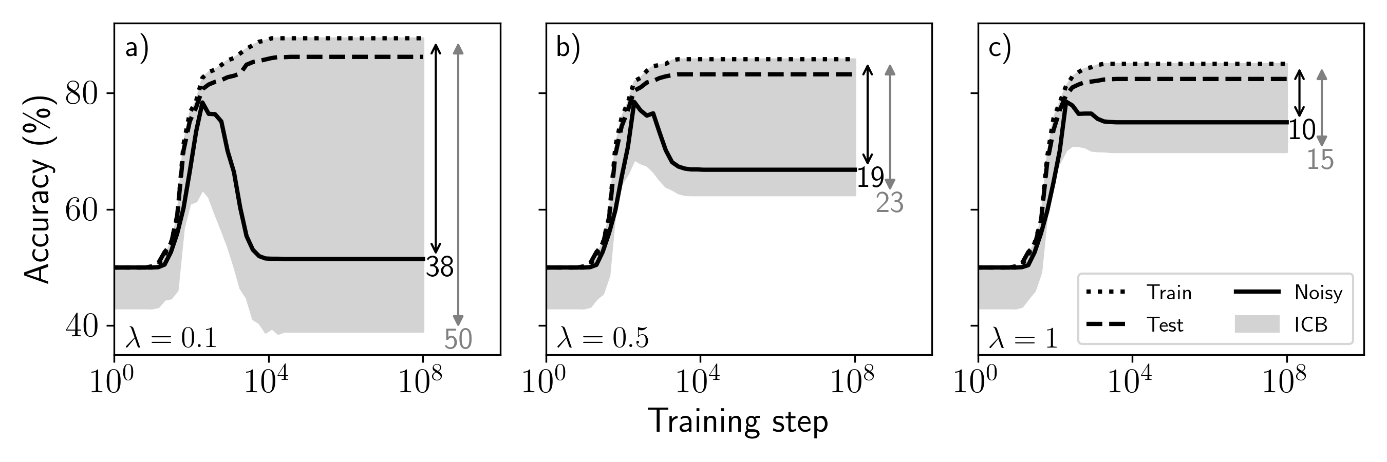
Figure 1: The ICB ( grey filled area) evaluated on the EuroSAT Pasture versus Sea-Lake binary classification task with 500 training samples and 2000 test samples at different regularization levels. At low regularization $\lambda=0.1$ (a), the ICB is vacuous with respect to standard generalization beyond $10^{4}$ training steps, but reflects the poor robust generalization for the “Noisy” test set with AWGN. Increasing the regularization to $\lambda=0.5$ (b) and $\lambda=1.0$ (c) reduces ICB and the AWGN GE. Arrows indicate the steady-state AWGN GE (black), and ICB ( grey) along with their respective values. See Fig. A5 for the corresponding upper and lower $I(X;Z)$ bounds for this experiment.

Illustrative example

Before presenting the main results, we examine ICB for a EuroSAT classification task using only $500$ training samples (Fig. 1). This is a challenging task, as tight MI and GE bounds are difficult to obtain for high-dimensional DNNs, particularly with few samples. For example, in (Dziugaite & Roy, 2017) $55000$ samples were used to obtain a $\approx 20\%$ GE bound for finite-width DNNs evaluated on MNIST.

We evaluate ICB throughout training from the first training step ($t=10^{0}$) until steady state when all accuracies stabilize ($t=10^{8}$). Shortly after model initialization ($t=10^{0}$ to $t=10^{1}$) the ICB is $<7\%$ (indicated by the height of the shaded region in Fig. 1) and the training and test accuracy are both at $50\%$ (GE $=0$). Here, ICB is non-vacuous, but also not necessarily interesting for this random-guessing phase. ICB increases as training is prolonged. At low regularization (Fig. 1 a), the ICB ultimately becomes vacuous (ICB $\approx 50\%$) around $10^{4}$ steps. However, although ICB is vacuous with respect to standard generalization in a), it reflects well the poor robust generalization when tested with AWGN (Gilmer et al., 2019). Increasing the regularization coefficient $\lambda$ reduces ICB from $50\%$ (a) to $23\%$ (b) and $15\%$ (c), and the robust GE from $38\%$ (a) to $19\%$ (b) and $10\%$ (c).

Both standard and robust GE are bounded at all times by ICB. The latter is, however, a coincidence, as the robust GE is subject to the arbitrary AWGN noise variance ($\sigma^{2}=\nicefrac{{1}}{{16}}$). The additive noise variance could be increased to increase the robust GE beyond the range bounded by ICB. More important than bounding the robust GE absolute percentage is that ICB captures the trend of robust generalization. Evaluating robustness effectively is error-prone and often assumes access to test data and a differentiable model (Athalye et al., 2018; Carlini et al., 2019). In contrast, we make no such assumptions here. The lack of robustness in Fig. 1 a) would have likely gone unnoticed by the practitioner. Either early stopping or increasing $\lambda$ reduce the ICB and robust GE as a potential solution—or a better trade-off between accuracy versus robustness (Tsipras et al., 2019). A caveat to this example is that only two metaparameters varied: the number of training steps $t$ and regularization $\lambda$. Next, we assess the ability of ICB to bound and rank GE for a broader range of metaparameters and datasets.

4.1 Bounding generalization error

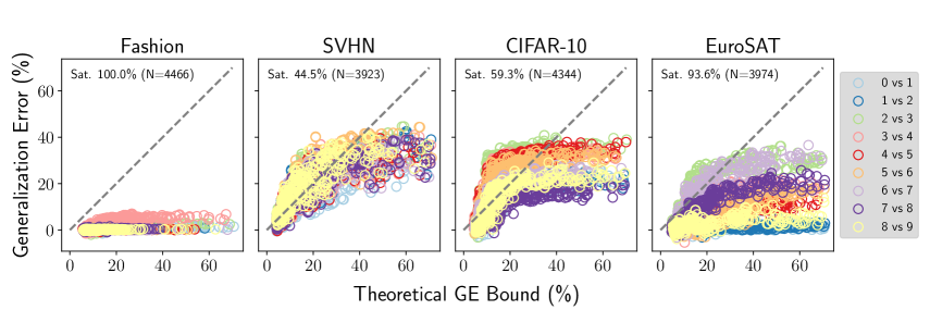
Figure 2: The ICB (“Theoretical GE Bound”) is plotted versus GE for FashionMNIST, SVHN, CIFAR, and EuroSAT datasets for Exp. A (§3.1). We refer to the percentage of models with GE $<$ ICB as the ICB satisfaction rate, which is annotated in the top left corner of each plot with format “Sat. % (N)”, where N denotes the number of valid experiments. Each binary classification task is assigned a unique colour to highlight inter-task differences in ICB satisfaction rate.

We refer to the percentage of tuples (ICB, GE) for which GE < ICB as the “ICB satisfaction rate”, or “Sat.” in plots. We expect $\approx 95\%$ of samples to satisfy this property as the bound is evaluated with $\delta=0.05$ or $95\%$ confidence. The overall ICB satisfaction rate with the respective number of valid experiments $N$ is listed in Table 1. Exp. B yielded greater $N$ than Exp. A primarily because it uses a different range for the regularization coefficient $\lambda$, resulting in larger $\lambda$ values. Since larger $\lambda$ is associated with more compression, Exp. B had fewer samples being discarded than in Exp. A due to $I_{\text{UB}}$ exceeding $\log(N_{\text{trn}})$. Otherwise, ICB satisfaction rates are similar, with SVHN performing slightly worse and CIFAR-10 slightly better for Exp. B versus Exp. A. These results also suggest that exploring nine binary classification tasks (Exp. A) serves as a useful approximation for the full set of all $45$ possible tasks (Exp. B). Next, we analyze how model performance influences the ICB satisfaction rate.

Table 1: Overall ICB satisfaction rate (Sat. %) with number of valid experiments $N$ in brackets. Results for Exp. A are also plotted in Figure 2; a more detailed breakdown of these results can be found in Table A6-10.

	MNIST	Fashion	SVHN	CIFAR	EuroSAT
Exp. A	$100\%~{}(2237)$	$100\%~{}(4466)$	$44.5\%~{}(3923)$	$59.3\%~{}(4344)$	$93.6\%~{}(3974)$
Exp. B	$100\%~{}(2250)$	$100\%~{}(4500)$	$27.0\%~{}(4500)$	$68.0\%~{}(4500)$	$95.0\%~{}(2221)$

When we restrict our scope to the best-performing models based on their test accuracy, the ICB satisfaction rate improves considerably. For example, models with test accuracy $\geq 80\%$ attain ICB satisfaction rates of $94\%~{}(N=682)$ for SVHN in Exp. B, and $99\%~{}(N=2812)$ for EuroSAT in Exp. A (Fig. A11(c)). For CIFAR-10 in Exp. B, we obtain $96\%~{}(N=591)$ by restricting to test accuracy $\geq 87\%$. The specific test accuracy thresholds were chosen to balance a trade-off between satisfying the ICB at $\approx 95\%$ and maximizing $N$. Although best-performing models are more likely to be deployed in practice, theoretical GE bounds generally prohibit access to a test set. Therefore, we next select models based on their training accuracy.

We refer to models that achieve $100\%$ accuracy on the training set as “overfitted”, consistent with prior use of this term by Belkin et al. (2018). Interestingly, restricting our analysis to overfitted models either improves or does not change ICB satisfaction rate for Exp. A. For MNIST, FashionMNIST, SVHN, and EuroSAT, overfitted models attain an ICB satisfaction rate of $100\%$ with $N=1970,1820,20,353$ respectively, while for CIFAR-10, the satisfaction rate remained below $95\%$, albeit it improved from $59.3\%~{}(N=4344)$ to $72.6\%~{}(N=876)$. Similar results were observed for Exp. B. Detailed plots for these results can be found in Figures A7, A8, A9, A10, A11 in the Appendix. The mostly excellent ICB satisfaction rates of the overfitted models are not due to trivially constant GE or ICB values; as can be seen in Figure 3, these models still have considerable variance w.r.t. both metrics despite their identical training accuracies.

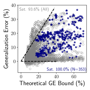
Figure 3: Theoretical GE bound (ICB) versus GE for EuroSAT (Exp. A). Overfitted models indicated by stars.

Inter-task differences were observed in terms of the ability of ICB to bound GE. For example for Exp. A, six of nine EuroSAT binary classification tasks always satisfied ICB ($N=2534)$, whereas two tasks in particular reduced the overall average. The satisfaction rate was only $68\%~{}(N=468)$ for the “2 vs. 3” task and $72\%~{}(N=475)$ for the “6 vs. 7” task (see Fig. A2 and Table A10 for detailed results). These tasks were unusual in that there was a strong inverse relationship between training error and GE, such that reducing the training error resulted in a steady increase in test error, with $\tau\approx-0.9$ for both tasks, compared to $\tau=-0.58$ for the “0 vs. 1” task. The negative correlation between training and test performance for the “2 vs. 3” task also resulted in a lower mean test accuracy ($70.2\pm 2.2\%~{}(N=467)$) compared to other tasks, e.g., “0 vs. 1” ($93.5\pm 5.3\%~{}(N=415)$), consistent with our previous observation that best-performing models generally satisfy ICB. We further investigated inter-task differences for EuroSAT Exp. B, for which all ${\binom{10}{2}}=45$ binary classification tasks were evaluated for 50 seeds each. For the two poorly performing tasks “2 vs. 3” and “6 vs. 7”, the ICB satisfaction rate was $78\%~{}(N=50)$ and $86\%~{}(N=50)$, respectively. For 34 of 45 tasks $(N=1913)$, ICB was satisfied for all seeds.

4.2 The randomization test

Zhang et al. (2017; 2021) proposed the “randomization test” after observing that DNNs easily fit random labels. They argue that useful generalization bounds ought to be able to distinguish models trained on natural versus randomized training labels, since generalization is by construction made impossible in the latter case. However, we cannot necessarily expect a theoretical GE bound to exactly hold for models trained on random labels, since the training and test sets are no longer drawn from the same distribution. We therefore pose the following questions: Q1: To what extent does the ICB correlate with the ability to fit random labels? Q2: Can ICB distinguish training sets with natural versus random labels? To address Q1, we aim to find metaparameters that reduce ICB and prevent models from fitting random training labels, while still permitting them to fit the natural training labels. This, however, introduces a potential for confounding if the metaparameter choice alone prevents the model from fitting random labels rather than ICB . For Q2, we hold all metaparameters constant and observe whether ICB changes for randomized training labels.

For simplicity, we consider a two-layer fully-connected ReLU network. We train the model to $t=\infty$ on the natural training set ($N_{\text{trn}}=1000$) with 20 different regularization values $\lambda$ in the range $10^{-4}\ \text{to}\ 10^{1}$. We measure Kendall’s $\tau$ ranking between the ICB evaluated on these models and their training accuracies when re-trained with random labels. We find that the ICB value obtained after training on natural labels is strongly correlated with the ability to fit random labels for all five datasets. Furthermore, competitive accuracy for natural training labels is preserved for three of five datasets in doing so (see Fig. 4).

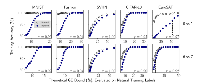
Figure 4: ICB often distinguishes between natural and randomized training sets. The accuracy w.r.t. the natural training labels (“Natural”) and randomized training labels (“Random”) is plotted versus the theoretical GE bound (ICB), which is evaluated on the natural training labels. Each data point in the plot corresponds to a unique regularization value $\lambda$, which in turn influences the ICB value: Small $\lambda$ leads to a large ICB value, while increasing $\lambda$ reduces the ICB and the ability to fit random labels, with the aim of preserving accuracy for natural training labels. The top row corresponds to the “0 vs. 1” task and bottom row the “6 vs. 7” task. Considerable separation between natural and random labels for MNIST, FashionMNIST, and EuroSAT is observed. Differences are harder to distinguish for SVHN and CIFAR-10, but still apparent. ICB is highly correlated with ability to fit random labels in all cases. The broken vertical line for EuroSAT indicates the ICB value for which there is at least a 10% difference in natural versus random training accuracy.

Table 2: ICB is larger when training to identical accuracy on random versus natural labels. Detailed results of the randomization test for EuroSAT are shown. The lower and upper MI bounds, $I_{\text{LB}}$ and $I_{\text{UB}}$, are included for comparison against $\log(N_{\text{trn}})\approx 6.91\ \text{nats}$. The columns $\text{ICB}_{\text{LB}}$ and $\text{ICB}_{\text{UB}}$ refer to whether $I_{\text{LB}}$ or $I_{\text{UB}}$ is taken as $I(X;Z)$ estimate, respectively. Columns “Train” and “Test” show the respective accuracy in $\%$. Both ICB values are larger for the random case when comparing rows with “Train”$=100.0$.

Natural Training Labels
$\lambda$	$I_{\text{LB}}$	$I_{\text{UB}}$	$\text{ICB}_{\text{LB}}$	$\text{ICB}_{\text{UB}}$	Train	Test	GE
$10^{-1}$	4.87	5.37	26.0	33.1	97.9	98.7	-0.8
$10^{-2}$	5.40	6.58	33.7	60.2	99.5	98.6	0.9
$10^{-3}$	5.78	7.40	40.5	90.4	100.0	97.5	2.5
Random Training Labels
$10^{-1}$	3.68	3.75	15.0	15.5	71.3	50.0	21.3
$10^{-2}$	5.28	5.67	31.7	38.5	89.7	50.0	39.7
$10^{-3}$	6.37	8.96	54.1	197.6	100.0	50.0	50.0

Surprisingly, $\text{ICB}_{\text{UB}}$ approximates the GE well even when the model is trained on random labels (Table 2). For $\lambda=0.1$, $\text{ICB}_{\text{UB}}=15.5\%$ compared to a GE of $21.3\%$. Next, for $\lambda=0.01$, $\text{ICB}_{\text{UB}}=38.5\%$ and GE is $39.7\%$. Last, for $\lambda=0.001$, $I_{\text{UB}}=8.96$, which is greater than $\log(N_{\text{train}})=6.91$ nats, therefore the corresponding $\text{ICB}_{\text{UB}}$ of $197.6\%$ should be discarded. In this case, substituting the “optimistic” lower estimate $\text{ICB}_{\text{LB}}=54.1\%\approx$ GE $=50\%$.

Intuitively, we expect $I(X;Z)$ to be smaller after training on natural labels, since training on random labels requires memorization of random data, i.e., the opposite of compression. However, note that to isolate the effect of the training label type on ICB, the training accuracy must also be controlled, as higher accuracy generally requires greater complexity and thus larger $I(X;Z)$. This intuition is consistent with our results, as both $I_{\text{LB}}$ and $I_{\text{UB}}$ increase monotonically with the training accuracy for both training label types (see Table 2).

Training with $\lambda=0.001$ allows models to perfectly fit both natural and randomized training sets (Table 2 column “Train” = $100\%$), which presents a suitable setting for evaluating whether ICB is sensitive to whether training labels are natural or random. Indeed, $I_{\text{LB}}$ is greater for random labels (6.37 vs. 5.78 nats), resulting in an increase of the optimistic theoretical GE bound, $\text{ICB}_{\text{LB}}$, from $40.5\%\ \text{to}\ 54.1\%$. The more pessimistic $\text{ICB}_{\text{UB}}$ increases even more dramatically from $90.4\%\ \text{to}\ 197.6\%$, which is beyond the valid range of GE ($0-100\%$).

The randomization test identifies tasks with low ICB satisfaction rate

Table 3: Ability of ICB to separate natural versus random training labels is a good predictor of ICB satisfaction rate by task. The row “$\text{ICB}_{\text{rand}}@X\%$” indicates the minimum ICB value for which a $X\%$ accuracy difference between natural and random labels is observed. The “Sat. (%)” column showing the ICB satisfaction rate is taken from §4.1, Exp. A. The column $\tau$ indicates the rank correlation between $\text{ICB}_{\text{rand}}@X\%$ and Sat. (%) over the nine tasks. Columns sorted by ascending order of $\text{ICB}_{\text{rand}}@X\%$.

	Task	2/3	6/7	3/4	7/8	4/5	5/6	0/1	1/2	8/9
EuroSAT	Sat. %	68	72	97	100	100	100	100	100	100	$\tau=0.76$
	$\text{ICB}_{\text{rand}}@10\%$	7.5	10.0	11.2	13.4	19.3	22.5	51.9	59.5	66.9
	Task	2/3	5/6	4/5	0/1	3/4	6/7	1/2	8/9	7/8
CIFAR-10	Sat. %	29	41	39	74	35	68	79	74	97	$\tau=0.65$
	$\text{ICB}_{\text{rand}}@5\%$	6.8	8.1	9.3	9.8	10.4	10.9	11.2	11.3	13.2

Recall from §4.1 that three binary classification tasks were responsible for reducing the ICB satisfaction rate below $100\%$ for EuroSAT: “2 vs. 3” (Sat. 68%), “6 vs. 7” (Sat. 72%), and “3 vs. 4” (Sat. 97%) for Exp. A. We observed that these were the same tasks for which ICB performed poorly on the randomization test. Specifically, we measured the minimum ICB value for which a $10\%$ or greater percentage difference was detected between the natural and random training-sets (see, e.g., the vertical broken line in Fig. 4). The “2 vs. 3” task required the smallest ICB ($7.5\%$) before the difference in label type became apparent. The “6 vs. 7” task had the next highest ICB of $10.0\%$, followed by “3 vs. 4” with $11.2\%$. The other six tasks—that have $100\%$ satisfaction rate—have strictly greater ICB (Table 3). Similar results are observed for CIFAR-10 using a smaller $5\%$ threshold as accuracies for natural and random labels were closer than for EuroSAT. The tasks with minimum (“2 vs. 3”) and maximum (“7 vs. 8”) satisfaction rate are the same tasks with the minimum and maximum $\text{ICB}_{\text{rand}}@5\%$. Therefore, the training-set based randomization test—which only required training a single model here—may be used to help identify when ICB performs well as a GE bound for a variety of models (e.g., the thousands of models that were considered in Exp. A). Our adaptation of the well-known randomization test complements the list of factors already identified in §4.1 as affecting ICB satisfaction rate.

4.3 Vacuous or non-vacuous?

Table 4: ICB is non-vacuous for best-performing models on five datasets. The GE (%) of a best-performing model is compared to ICB for each dataset. The column $N_{\text{trn}}$ indicates the number of training samples, which was a metaparameter for the first experiment (§3.1, Exp. A), and a constant for the second experiment (§3.2, Exp. B).

	Exp. A, $t=\{10^{2},\dots,10^{6}\}$					Exp. B, $t=\infty$
Dataset	Train	Test	GE	ICB	$N_{\text{trn}}$	Train	Test	GE	ICB	$N_{\text{trn}}$
MNIST	100.0	100.0	0.0	11.2	931	99.9	99.9	0.0	12.1	1000
Fashion	99.9	100.0	-0.1	7.2	1112	99.9	100.0	-0.1	8.1	1000
SVHN	98.8	74.2	24.6	28.0	1564	100.0	90.8	9.3	21.1	2000
CIFAR	94.8	89.2	5.6	7.6	1966	99.2	93.8	5.4	11.3	2000
EuroSAT	97.8	98.7	-0.9	25.6	1979	100.0	100.0	0.0	22.6	1000

Models with high test accuracy are the more likely to be deployed in practice. To evaluate whether ICB is non-vacuous and close enough to GE to aid model comparison, for each dataset we selected the model with the smallest ICB value among the top-three most accurate models. The ICB values are considerably less than $50\%$ in all cases, satisfying the basic definition of non-vacuous for a binary classification task (Table 4). For Exp. A, the smallest difference between ICB and GE occurred for the CIFAR dataset, with a GE of $5.6\%$ compared to an ICB value of $7.6\%$ for $1966$ training samples (Table 4, Exp. A). The greatest ICB value occurred for SVHN ($28.0\%$), however the GE was also large in this case ($24.6\%$).

For Exp. B, both ICB and GE decrease for SVHN (Table 4, Exp. B)) relative to Exp. A. For CIFAR, a similar GE of $\approx 5\%$ is attained as in Exp. A, but with a greater ICB by $3.7\%$. This may be due to the training accuracy increasing by $4.4\%$ from $94.8\%$ (Exp. A) to $99.2\%$ (Exp. B). In summary, not only is ICB non-vacuous, it is close enough to GE to perform model comparisons.

4.4 Relationship between theoretical bound and generalization error

Here, we evaluate the ability of ICB to rank GEs in terms of Kendall’s rank correlation coefficient, $\tau$. Our analysis of correlation between a complexity metric and empirical GE is inspired by a previous study and NeurIPS competition (Jiang* et al., 2019; Jiang et al., 2021). Figure A13 helps motivate the use of the ICB for ranking GE rather than using its constituent complexity metric $I(X;Z$), based on a subset of Exp. B metaparameters.

An issue with correlation analysis is that the training-set classification error or proxy loss can serve as a good predictor of GE, therefore Jiang* et al. (2019) train models to a fixed training loss to control for confounding effects. However, fixing the training loss limits the extent of metaparameter exploration. For example, a complexity metric or GE bound may rank GEs of overfitted models well, but perform poorly for early-stopping. To maintain a broad scope, we follow both Exp. A & B procedures and treat the train-set accuracy as a baseline for comparison against ICB, then evaluate overfitted models separately.

Table 5: Kendall’s $\tau$ ranking for three GE types: Clean, AWGN and FGSM for models that obtain zero training error. The number of models is indicated by the $N$ column. NB: The “–” entries for SVHN had $p>0.05$ when computing $\tau$ and were therefore discarded.

Dataset	$N$	Clean	AWGN	FGSM
MNIST	2329	0.27	0.30	0.29
Fashion	1820	0.39	0.42	0.41
SVHN	20	0.32	–	–
CIFAR	876	0.19	0.20	0.12
EuroSAT	353	0.33	0.38	0.29

Two perturbed test sets help measure correlations between ICB and robust GE; as perturbations we use AWGN (Gilmer et al., 2019) and FGSM (Goodfellow et al., 2015). These perturbations are appropriate for evaluating the robustness of infinite-width networks trained by GD, which behave as linear functions of their parameters (Lee et al., 2019). It can be shown that a classifier’s error rate for a test set corrupted by AWGN determines the distance to the decision boundary for linear models (Fawzi et al., 2016) and serves as a useful guide for DNNs (Gilmer et al., 2019). For AWGN, we use a Gaussian variance $\sigma^{2}=\nicefrac{{1}}{{16}}$ for EuroSAT and $\sigma^{2}=\nicefrac{{1}}{{4}}$ for the other datasets. For FGSM, we use a $\ell_{\infty}$-norm perturbation of size $4/255$ for inputs $x\in[-1,+1]$.

In terms of ranking (Clean, AWGN, FGSM) GEs by aggregating all nine tasks for Exp. A, ICB performs better than the training accuracy baseline for MNIST (Table A6) and FashionMNIST (Table A7); slightly worse than the baseline for SVHN (Table A8) and EuroSAT (Table A10); roughly on par with the baseline for CIFAR (Table A8). All overfitted models from the Exp. A procedure have a positive $\tau$-ranking between ICB and the three GE types for all datasets (Table 5). Thus, ICB outperforms the training accuracy baseline ($\tau=0$) here.

For Exp. B, there was considerable variance in $\tau$-rankings among the $45$ binary classification tasks for each dataset. Although the median ranking was positive for all datasets, the baseline achieves a higher median ranking than ICB for all three error types (Clean, AWGN, FGSM) (Fig. A12).

5 Discussion

Our results show that the ICB serves as a non-vacuous generalization bound, which we verified in the case of infinite-width networks. Furthermore, we performed a broader evaluation than is typically considered for theoretical GE bounds: i) We attempted to falsify ICB by evaluating it throughout training, rather than at a specific number of epochs or training loss value. ii) We varied the number of training samples and classification labels, compared to a static train/test split. iii) We considered robust GE in addition to standard GE. iv) Our experiments were performed on five datasets.

ICB was consistently satisfied at the expected $95\%$ rate for models with at least $70-80\%$ test accuracy, which is encouraging since accurate models are more likely to be deployed in practice. It is, however, more helpful to threshold by training accuracy to establish a regime in which ICB always works well, since one does not assume access to held-out data when evaluating generalization bounds. The relationship between training accuracy and the percentage of models satisfying ICB was unfortunately weaker, despite being nearly $100\%$ for overfitted models. Nonetheless, ICB was satisfied at a high rate of at least $92\%$ of the time for three of five datasets (MNIST, FashionMNIST, and EuroSAT) without excluding any models by accuracy, and the training label randomization test was sensitive to tasks where ICB wasn’t satisfied.

Compared to a simple training accuracy baseline, ICB performed well at ranking GE when the classification task was allowed to vary (e.g., grouping errors for 1 vs. 2 classification with those for a 2 vs. 3 task), or when the training accuracy was fixed at $100\%$. ICB, however, did not always outperform the training accuracy baseline for specific tasks and when GEs took a large range. However, a limited error ranking ability is not necessarily disqualifying for a generalization bound. It is unclear to what extent a generalization bound ought to be able to rank GEs, given that it is by definition merely an upper bound on the error. For example, GEs of $1\%$ and $29\%$ are both compatible with a bound of $30\%$, which would contribute to a poor ranking in terms of Kendall’s $\tau$. When varying one metaparameter at a time—in particular the diagonal regularization coefficient—a strong monotonic relationship is observed between ICB and robust errors AWGN and FGSM.

Relevance to deep learning

One should use caution before extrapolating our conclusions based on infinite-width networks to finite-width DNNs. The ability of infinite-width networks to approximate their finite-width counterparts is reduced with increasing training samples (Lee et al., 2019), regularization (Lee et al., 2020), and depth (Li et al., 2021). Nevertheless, the infinite-width framework has allowed us to demonstrate the practical relevance of the ICB for an exciting family of models as a first step. It has been argued that understanding generalization for shallow kernel learning models is essential to understanding generalization behaviour of deep networks. Kernel learning and deep learning share the ability to exactly fit their training sets yet still generalize well, a phenomenon that other bounds fail to explain (Belkin et al., 2018). We leave the study of ICB in the context of finite-width DNNs to future work, which may require alternative MI estimation techniques.

6 Related Work

Kernel-regression generalization error

Canatar et al. (2021b) derived an analytical expression for the generalization MSE of kernel regression models using a replica method from statistical mechanics. Their predictions show excellent agreement with the empirical GE of NTK models on MNIST and CIFAR datasets as a function of the training sample size. Furthermore, their method is sensitive to differences in difficulty between similar classification tasks, e.g., showing that MNIST “0 vs 1” digit classification is easier to learn than “8 vs 9”. Their method has also been extended to predict out-of-distribution generalization error (Canatar et al., 2021a).

An alternative method is the Leave-One-Out (LOO) error estimator (Lachenbruch, 1967). LOO is generally impractical for deep learning due to the computational effort required to train $n$ DNNs from scratch on $n$ different training sets. However, Bachmann et al. (2021) proposed a closed-form expression for the LOO estimator for a single kernel regression model trained once on the full training set. Their estimator shows excellent agreement with test MSE and accuracy for a five-layer ReLU NTK model trained on MNIST and CIFAR. While Bachmann et al. averaged results over five training sets of size $500-20000$, we only draw a single training set of $250-2000$ samples for each set of metaparameters. Our choice was made to reflect a practical “small data” scenario, where GE has to be bounded using a modest set of labeled data. As a result, however, our GE and ICB estimates have greater variance than those of Bachmann et al..

In this work, we used the infinite-width limit of neural networks for convenience and as a first step to assess the efficacy of ICB; we did not set out to find optimal generalization bounds for kernel regression. An advantage of ICB is that it only requires access to $I(X;Z)$—a black-box statistic applicable to a wide variety of models beyond kernel regression. Therefore, ICB may become increasingly relevant for deep learning using MI estimators with different assumptions, e.g., with distributional constraints on weight matrices (Gabrié et al., 2018) or log-Gaussian corrections for infinite depth-and-width limits (Li et al., 2021).

Generalization bounds for deep learning

Dziugaite & Roy (2017) develop a PAC-Bayes GE bound and evaluated it on a MNIST binary classification task (classes $\{0,\dots,4\}$ vs. $\{5,\dots,9\}$) using the complete training set ($N_{\text{train}}=55k$) and a ReLU fully-connected NN with 2-3 layers. Although their bound was non-vacuous ($\approx 20\%$), it was several times larger than the error estimated on held-out data ($<1\%$). A direct comparison with our work is difficult, as we did not use finite-width DNNs. We showed that the ICB yields a smaller ($\approx 10\%)$ bound from less than $2000$ samples for MNIST binary classification tasks. The PAC-Bayes bound was also evaluated at a single point during training at 20 epochs, whereas we evaluated ICB from initialization to convergence to check for violations and tightness of the bound.

Zhou et al. (2019) proposed a PAC-Bayes generalization bound based on the compressed size of a DNN after pruning and quantization. They obtain a GE bound of $46\%$ for MNIST and $96-98\%$ for ImageNet. The measure of compression used by Zhou et al. (2019) should not be confused with input compression in terms of MI in this study. The bounds of Dziugaite & Roy (2017) and Zhou et al. (2019) concern model complexity, whereas ICB is concerned with input data compression by the hidden layers. Both Dziugaite & Roy and Zhou et al. retrained models from scratch to optimize their bound for best results, whereas we did not modify any aspect of the standard gradient descent training procedure or NTK architecture to be more aligned with ICB.

Input compression and deep learning

Saxe et al. (2018) observed a lack of compression in ReLU networks and argued that compression must be unrelated to generalization in DNNs, since it is known that ReLU networks generalize well. However, their binning procedure based on (Paninski, 2003) involves metaparameters that influence entropy and MI estimation. Other works reported input compression in linear regression (Chechik et al., 2005) and finite-width ReLU DNNs using adaptive binning estimators (Chelombiev et al., 2019). We use MI bounds free from such metaparameters and observe input compression regardless of the nonlinearity type, consistent with Shwartz-Ziv & Alemi (2020).

The construction of invertible DNNs (Jacobsen et al., 2018) that generalize well has raised questions about a possible connection between compression and generalization of DNNs. However, to the best of our knowledge there have been few attempts to accurately measure information-theoretic compression in deterministic invertible networks. Although MI diverges for deterministic networks (Goldfeld et al., 2019), input compression may be observed in principle by substituting entropy for MI (Strouse & Schwab, 2016). This noise-free limit has also been studied in the context of information maximization (Bell & Sejnowski, 1995). We are excited about future work that may shed light on input compression phenomena and the challenging case of deep, deterministic, finite-width NNs.

7 Conclusion

We assessed the ICB along three axes of performance: tightness of the bound (e.g., vacuous or non-vacuous), percentage of trials satisfying the bound, and ranking generalization errors. Our empirical results show that input compression serves as a simple and effective generalization bound, complementing previous theoretical evidence. Additionally, ICB can help pinpoint interesting failures of robust generalization that go undetected by standard generalization metrics. An important consequence of the ICB with respect to NAS is that bigger is not necessarily better, at least in terms of the information complexity of infinite-width networks. Equally if not more important than the architecture are the metaparameters and duration of model training, all of which influence input compression. Consistent with Occam’s razor, less information complexity—or more input compression—yields more performant models, reducing the upper bound on generalization error. We conclude that input compression, which is data-centric, is a more effective complexity metric than model-centric proxies like the number of parameters or depth.

Acknowledgments

This research was developed with funding from the Defense Advanced Research Projects Agency (DARPA). The views, opinions and/or findings expressed are those of the author and should not be interpreted as representing the official views or policies of the Department of Defense or the U.S. Government. Graham W. Taylor and Angus Galloway also acknowledge support from CIFAR and the Canada Foundation for Innovation. Angus Galloway also acknowledges supervision by Medhat Moussa. Resources used in preparing this research were provided, in part, by the Province of Ontario, the Government of Canada through CIFAR, and companies sponsoring the Vector Institute: http://www.vectorinstitute.ai/#partners. Anna Golubeva is supported by the National Science Foundation under Cooperative Agreement PHY-2019786 (The NSF AI Institute for Artificial Intelligence and Fundamental Interactions, http://iaifi.org/). Mihai Nica is supported by an NSERC Discovery Grant.

Appendix A Appendix

A.1 Lower bound on MI

We may lower bound $I(X;Z)$ using a bound of similar form as equation 2 based on a batch of $N$ samples:

$$I(X;Z)\geq\mathbb{E}\left[\frac{1}{N}\sum_{i=1}^{N}\log\frac{p(z_{i}|x_{i})}{\frac{1}{N}\sum_{j}p(z_{i}|x_{j})}\right]=I_{\text{LB}}\,,$$ (5)

where the expectation is taken over $N$ independent samples from the joint distribution $\prod_{j}p(x_{j},z_{j})$. The main difference between this bound and equation 5 is the inclusion of $p(z_{i}|x_{i})$ in the denominator.

A.2 Illustrative example and filtering MI

We empirically verified that equation 5 and equation 2 yield similar results when $I_{\text{UB}}<\log(N_{\text{trn}})$ (Fig. A5).

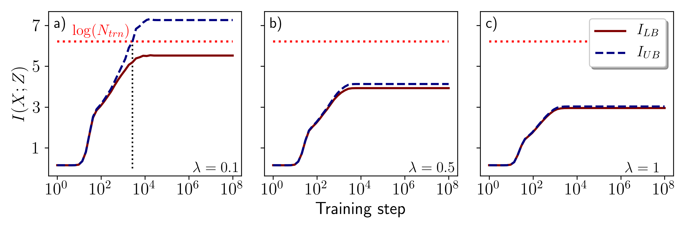
Figure 5: We plot $I(X;Z)$ upper (2) and lower (5) bounds corresponding to the illustrative EuroSAT example (Figure 1). Increasing the regularization to $\lambda=0.5$ in b) and $\lambda=1.0$ in c) reduces MI below $\log(N_{\text{trn}})$. Samples to the right of the vertical line in a) where $I_{UB}$ crosses $\log(N_{\text{trn}})$ are discarded for the main analyses. NB: We use natural units (“Nats” or “Shannons”) for $I(X;Z)$ here, but we convert to bits when evaluating the ICB.

A.3 Bounding generalization throughout training

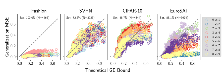
Figure 6: ICB is plotted versus GE for FashionMNIST, SVHN, CIFAR-10, and EuroSAT datasets. The ICB satisfaction rate is annotated in the top left corner of each plot with format “ICB % (N)”. Each binary classification task is assigned a unique colour to highlight inter-task differences in ICB satisfaction rate. See Figure 2 of §4.1 for the corresponding Figure with GE expressed in terms of classification error rather than MSE. NB: Results for MNIST omitted from Figure as they were similar to FashionMNIST.

Loss function

We considered GE in terms of MSE in addition to classification error (Fig. A6). This change results in no difference in the overall ICB Sat. for FashionMNIST, an improvement for SVHN from $44.5\%$ to $72.6\%$, and a small decrease for CIFAR-10 from to $59.3\%$ to $48.7\%$ as well as for EuroSAT from $93.6\%$ to $88.1\%$.

Activation function

Overall, ReLU networks satisfied ICB more frequently than Erf networks (Table A11).

The following caption applies to Tables A6-10.

Kendall’s $\tau$ ranking for three generalization error types: Clean, AWGN and FGSM by training accuracy “Train (baseline)” and ICB are presented. One hundred random seeds are used to draw different metaparameters uniform random for each task, for which models are evaluated five (5) times each during training resulting in a maximum of 500 samples per task. The number of valid samples out of 500, i.e., those with $I_{\text{UB}}(X;Z)\leq\log(N_{\text{train}})$ is indicated in the $N_{\text{valid}}$ column. ICB % indicates the percentage of samples that satisfy the ICB, i.e., Clean generalization error $\leq$ ICB. Entries in the “Row average” row are obtained by simply averaging across the nine (9) tasks. Kendall’s $\tau$ values for the “Overall” row may differ substantially from “Row average” as this corresponds to aggregating all raw data points and considering them as one task before calculating $\tau$. Bold is used to denote whether the baseline or ICB achieve a better ranking of generalization errors.

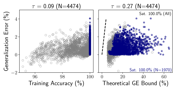
(a)

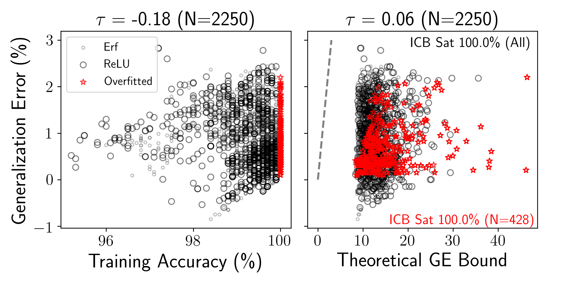
(b)

Figure 7: 7(a)) MNIST models evaluated throughout training, 7(b)) models evaluated at steady state $t=\infty$.

Table 6: Kendall’s $\tau$ ranking for MNIST. See complete caption in §A.3.

Details			Train (baseline)			ICB
Task	$N_{\text{valid}}$	ICB %	Clean	AWGN	FGSM	Clean	AWGN	FGSM
0 vs. 1	499	100%	0.36	0.37	0.35	0.10	0.09	0.10
1 vs. 2	498	100%	0.39	0.65	0.33	0.34	0.52	0.32
2 vs. 3	497	100%	0.42	0.57	0.46	0.42	0.55	0.46
3 vs. 4	500	100%	0.27	0.32	0.24	0.22	0.29	0.23
4 vs. 5	493	100%	0.19	0.31	0.14	0.19	0.32	0.17
5 vs. 6	497	100%	0.49	0.59	0.51	0.44	0.53	0.46
6 vs. 7	498	100%	0.29	0.27	0.23	0.17	0.23	0.17
7 vs. 8	498	100%	0.35	0.44	0.32	0.38	0.46	0.38
8 vs. 9	494	100%	0.42	0.56	0.44	0.38	0.52	0.42
Row average		100%	0.35	0.45	0.34	0.29	0.39	0.30
Overall			0.09	0.12	0.03	0.27	0.31	0.24

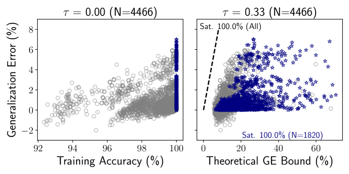
(a)

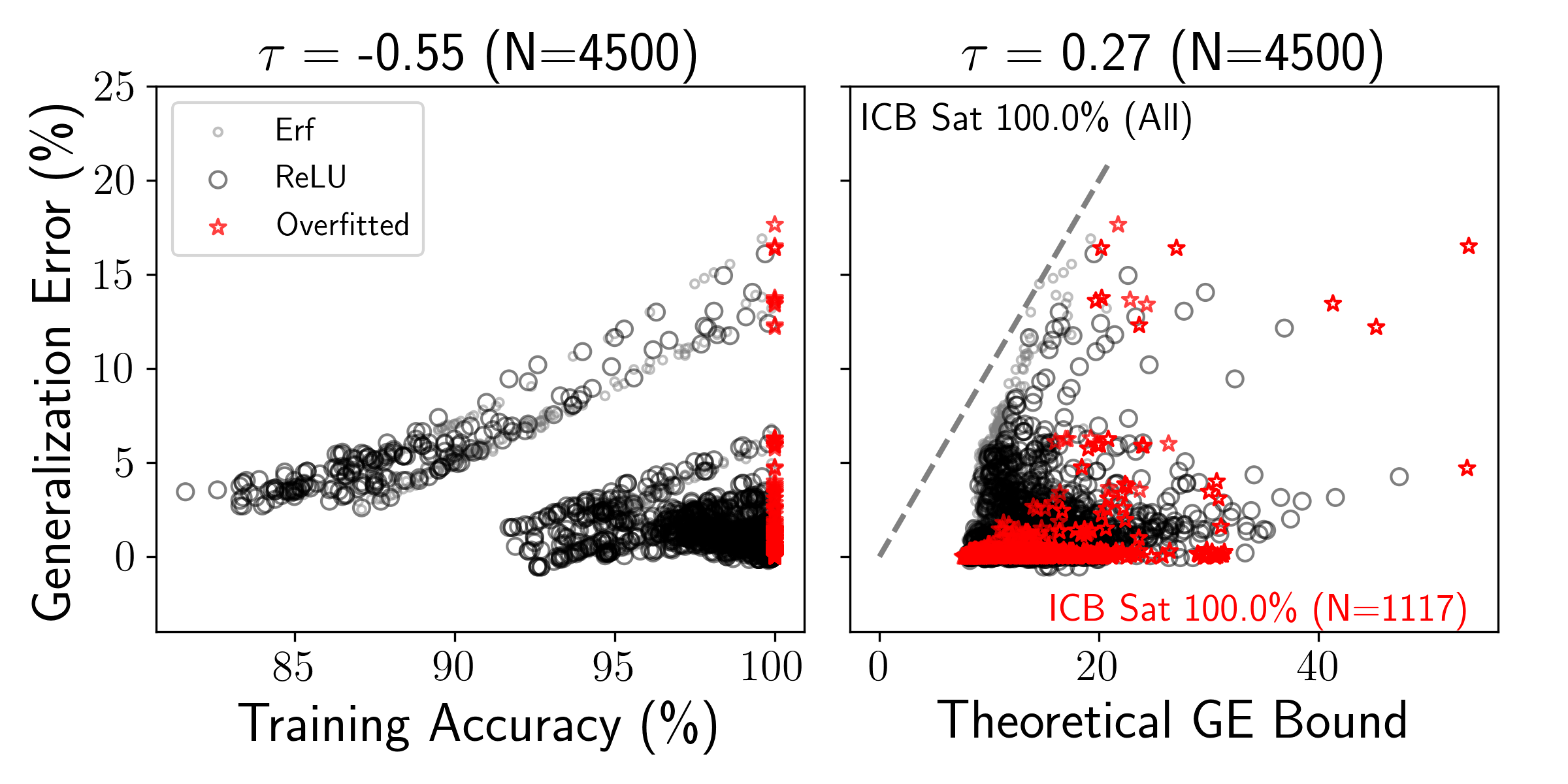
(b)

Figure 8: FashionMNIST models evaluated 8(a)) throughout training and 8(b)) at steady state $t=\infty$.

Table 7: Kendall’s $\tau$ ranking for FashionMNIST. See complete caption in §A.3.

Details			Train (baseline)			ICB
Task	$N_{\text{valid}}$	ICB %	Clean	AWGN	FGSM	Clean	AWGN	FGSM
0 vs. 1	250	100%	0.59	0.67	0.66	0.46	0.57	0.54
1 vs. 2	248	100%	0.48	0.59	0.55	0.42	0.50	0.46
2 vs. 3	247	100%	0.76	0.80	0.80	0.57	0.60	0.61
3 vs. 4	243	100%	0.78	0.82	0.84	0.67	0.66	0.66
4 vs. 5	250	100%	0.04	-0.02	-0.11	0.08	-0.02	0.00
5 vs. 6	249	100%	0.18	0.15	0.04	0.13	0.17	0.06
6 vs. 7	250	100%	0.35	0.26	0.23	0.17	0.16	0.12
7 vs. 8	250	100%	0.37	0.52	0.31	0.35	0.46	0.35
8 vs. 9	250	100%	0.40	0.29	0.38	0.20	0.11	0.20
Row average		100%	0.44	0.45	0.41	0.34	0.35	0.34
Overall			-0.02	-0.03	-0.09	0.33	0.33	0.31

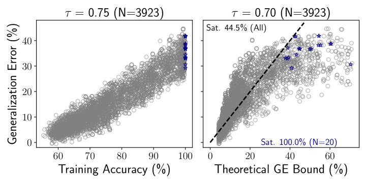
(a)

(b)

Figure 9: 9(a)) SVHN models evaluated throughout training, 9(b)) models evaluated at steady state $t=\infty$.

Table 8: Kendall’s $\tau$ ranking for SVHN. See complete caption in §A.3.

Details			Train (baseline)			ICB
Task	$N_{\text{valid}}$	ICB %	Clean	AWGN	FGSM	Clean	AWGN	FGSM
0 vs. 1	443	71%	0.75	0.85	0.80	0.70	0.74	0.63
1 vs. 2	432	33%	0.81	0.90	0.84	0.74	0.73	0.66
2 vs. 3	440	34%	0.82	0.89	0.83	0.74	0.73	0.64
3 vs. 4	438	44%	0.82	0.90	0.83	0.73	0.75	0.67
4 vs. 5	441	60%	0.81	0.90	0.83	0.76	0.75	0.65
5 vs. 6	442	25%	0.86	0.92	0.86	0.73	0.72	0.65
6 vs. 7	429	49%	0.79	0.90	0.83	0.72	0.71	0.63
7 vs. 8	440	48%	0.78	0.88	0.83	0.73	0.73	0.65
8 vs. 9	438	32%	0.84	0.91	0.82	0.74	0.73	0.63
Row average		44%	0.81	0.89	0.83	0.73	0.73	0.65
Overall			0.75	0.85	0.80	0.71	0.72	0.64

(a)

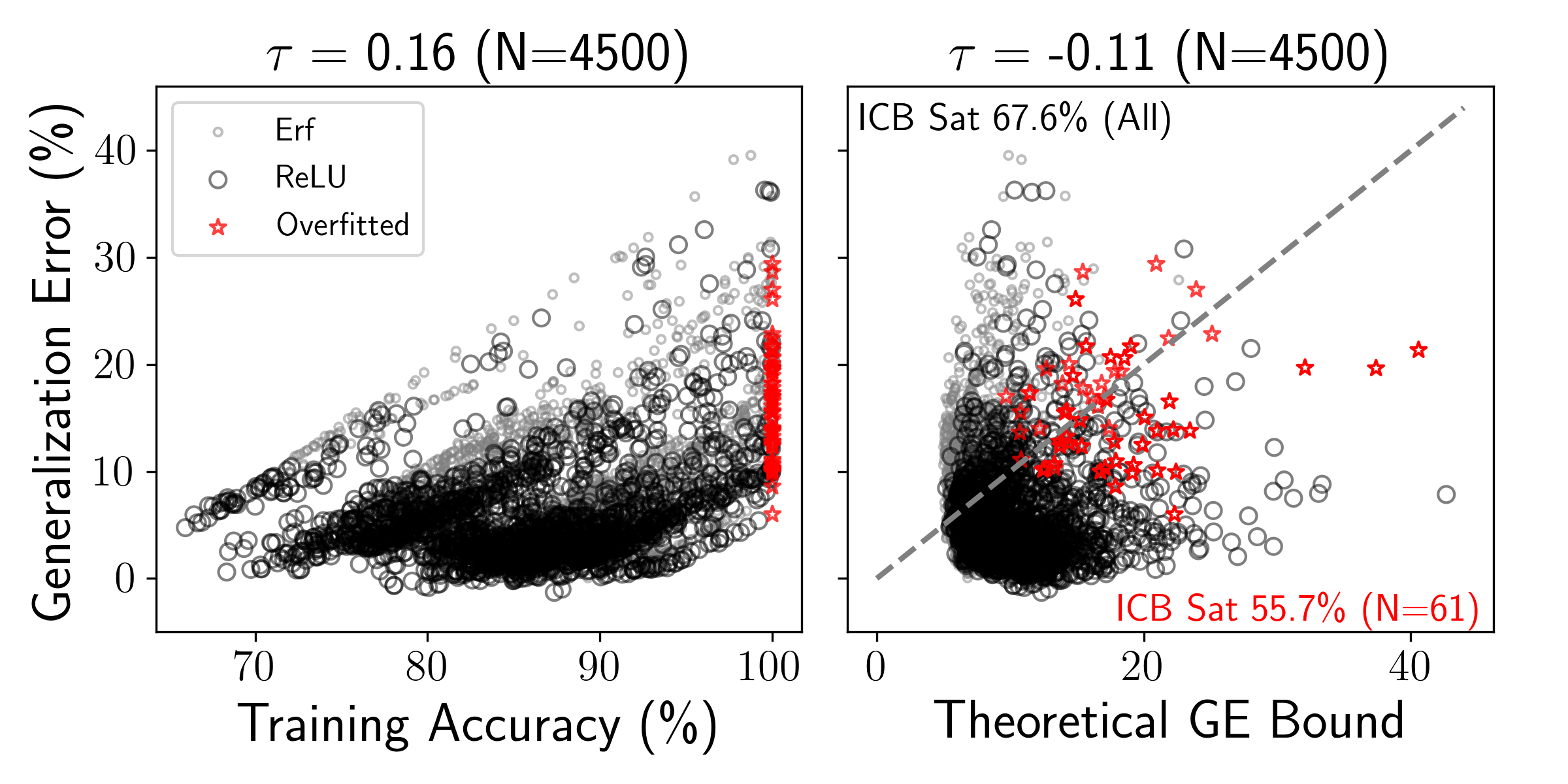
(b)

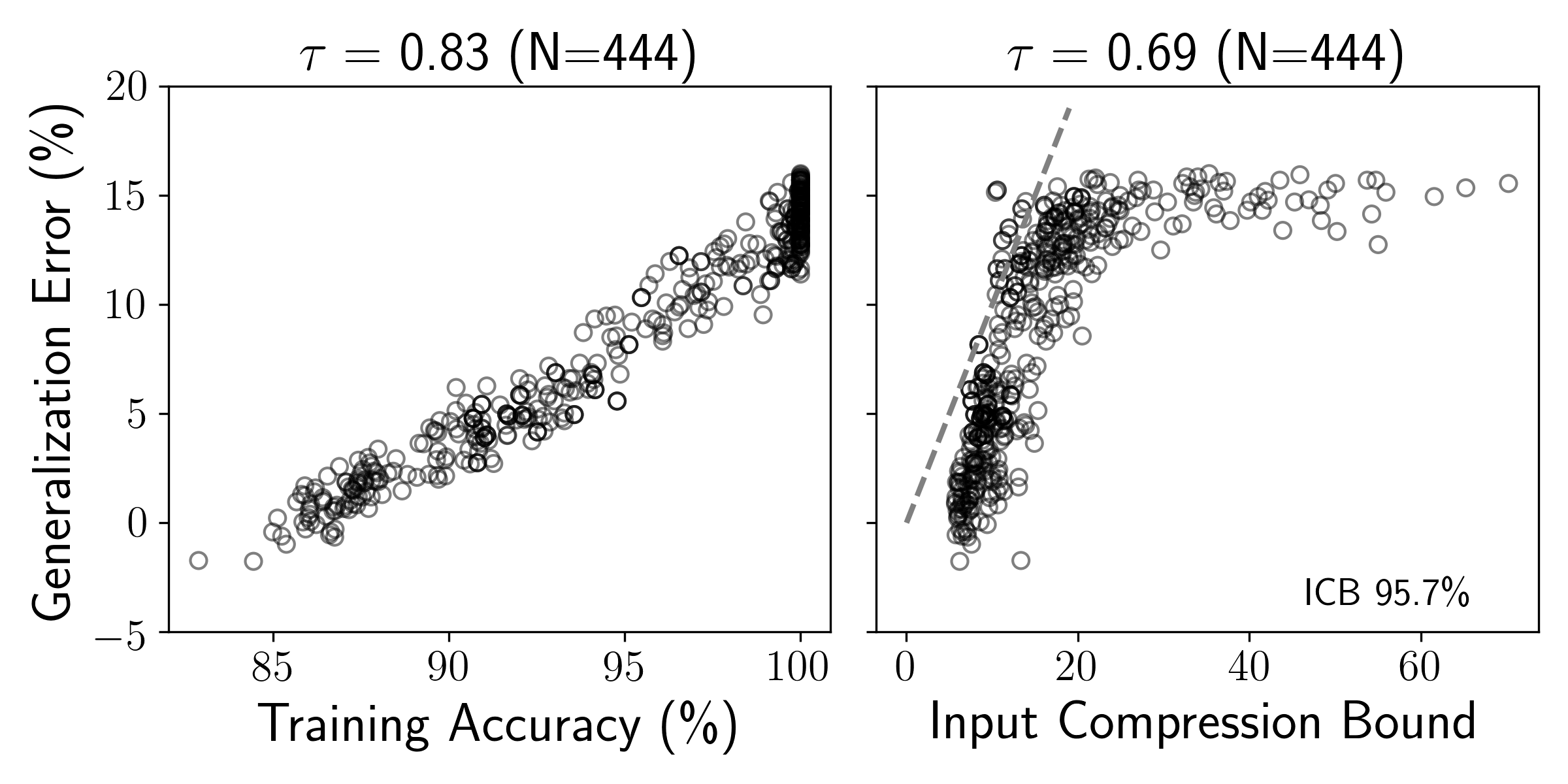
(c)

Figure 10: 10(a)) CIFAR models evaluated throughout training, 10(b)) models evaluated at steady state $t=\infty$, 10(c)) select models from 10(a)) with $\geq 84\%$ test accuracy.

Table 9: Kendall’s $\tau$ ranking for CIFAR-10. See complete caption in §A.3.

Details			Train (baseline)			ICB
Task	$N_{\text{valid}}$	ICB %	Clean	AWGN	FGSM	Clean	AWGN	FGSM
0 vs. 1	482	74%	0.85	0.88	0.87	0.72	0.73	0.69
1 vs. 2	489	79%	0.84	0.87	0.87	0.75	0.75	0.70
2 vs. 3	487	29%	0.88	0.90	0.86	0.77	0.76	0.68
3 vs. 4	480	35%	0.86	0.88	0.85	0.76	0.76	0.69
4 vs. 5	472	39%	0.89	0.90	0.87	0.76	0.75	0.68
5 vs. 6	481	41%	0.86	0.89	0.86	0.76	0.75	0.67
6 vs. 7	487	68%	0.82	0.85	0.84	0.78	0.77	0.70
7 vs. 8	488	97%	0.82	0.86	0.84	0.71	0.71	0.66
8 vs. 9	486	74%	0.85	0.88	0.87	0.75	0.74	0.71
Row average		59%	0.85	0.88	0.86	0.75	0.75	0.69
Overall			0.61	0.65	0.64	0.62	0.65	0.62

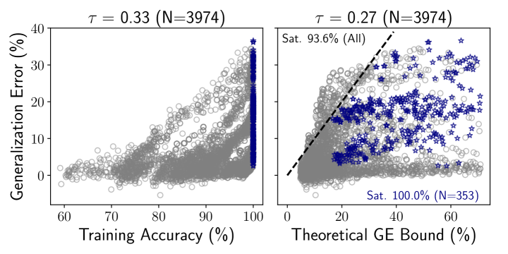
(a)

(b)

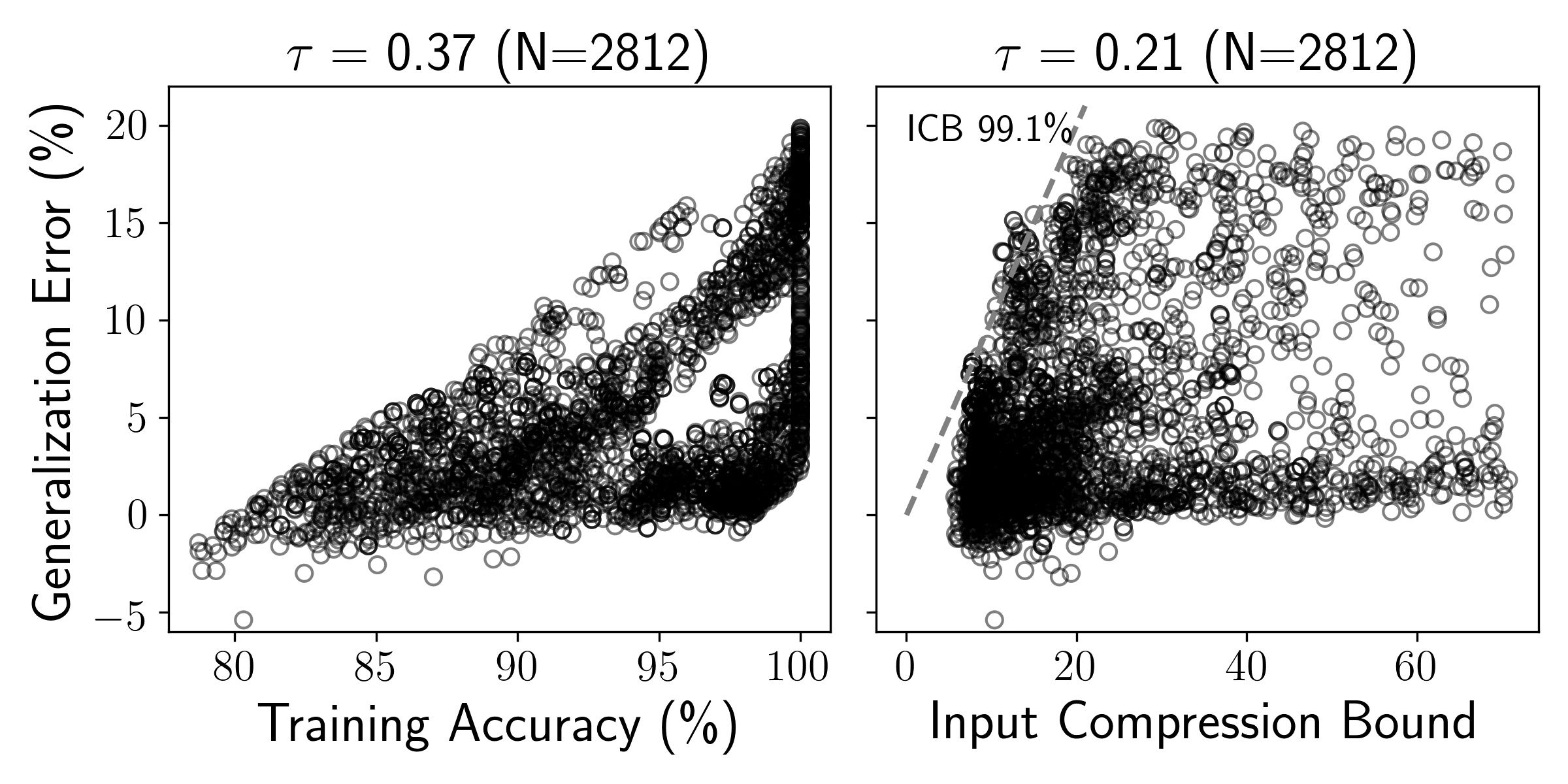
(c)

Figure 11: 11(a)) EuroSAT model evaluated throughout training, 11(b)) models evaluated at steady state $t=\infty$, 11(c)) select models from 11(a)) with $\geq 80\%$ test accuracy.

Table 10: Kendall’s $\tau$ ranking for EuroSAT. See complete caption in §A.3.

Details			Train (baseline)			ICB
Task	$N_{\text{valid}}$	ICB %	Clean	AWGN	FGSM	Clean	AWGN	FGSM
0 vs. 1	414	100%	0.26	0.40	0.37	0.25	0.43	0.38
1 vs. 2	389	100%	0.30	0.59	0.50	0.24	0.54	0.37
2 vs. 3	468	68%	0.86	0.91	0.76	0.77	0.78	0.60
3 vs. 4	490	97%	0.86	0.86	0.83	0.72	0.72	0.65
4 vs. 5	485	100%	0.62	0.61	0.77	0.70	0.70	0.68
5 vs. 6	444	100%	0.78	0.79	0.80	0.68	0.67	0.62
6 vs. 7	475	72%	0.89	0.88	0.80	0.74	0.74	0.62
7 vs. 8	467	100%	0.80	0.83	0.82	0.77	0.77	0.67
8 vs. 9	335	100%	0.47	0.74	0.63	0.40	0.61	0.51
Row average		93%	0.65	0.73	0.70	0.59	0.66	0.57
Overall			0.34	0.36	0.33	0.26	0.28	0.28

A.4 Bounding generalization at steady state

Results for bounding the generalization error at steady state are summarized in Table A11.

Table 11: Results for bounding generalization error across five (5) datasets with Input Compression Bound (ICB). For each dataset, all ${\binom{10}{2}}=45$ binary label combinations are evaluated for $S=25-50$ meta-parameter combinations drawn uniform random. The ICB % column indicates the percentage of $N_{\text{trials}}$ that satisfy the ICB, where $N_{\text{trials}}={\binom{10}{2}}\times S$. The mean and maximum Clean generalization error is indicated by “Mean Err” and “Max Err” respectively. The training set sample size is indicated by $N_{\text{train}}$. A test set with $N_{\text{test}}=2000$ is used in all cases except for EuroSAT ($N_{\text{test}}=1000$). Results are broken down by nonlinearity type as Erf resulted in ICB being satisfied less often.

					Error
Dataset	$N_{\text{train}}$	$N_{\text{trials}}$	Arch	ICB %	Mean Err	Max Err
MNIST	1000	1125	Erf	100.0	0.8	2.4
			ReLU	100.0	0.8	2.8
Fashion	1000	2250	Erf	99.9	1.3	16.5
			ReLU	100.0	1.4	17.7
SVHN	2000	2250	Erf	0.3	14.1	35.7
			ReLU	52.8	7.4	24.8
CIFAR-10	2000	2250	Erf	47.6	8.5	39.5
			ReLU	86.5	5.4	36.3
EuroSAT	1000	1125	Erf	90.0	2.1	22.9
			ReLU	99.5	5.1	43.0

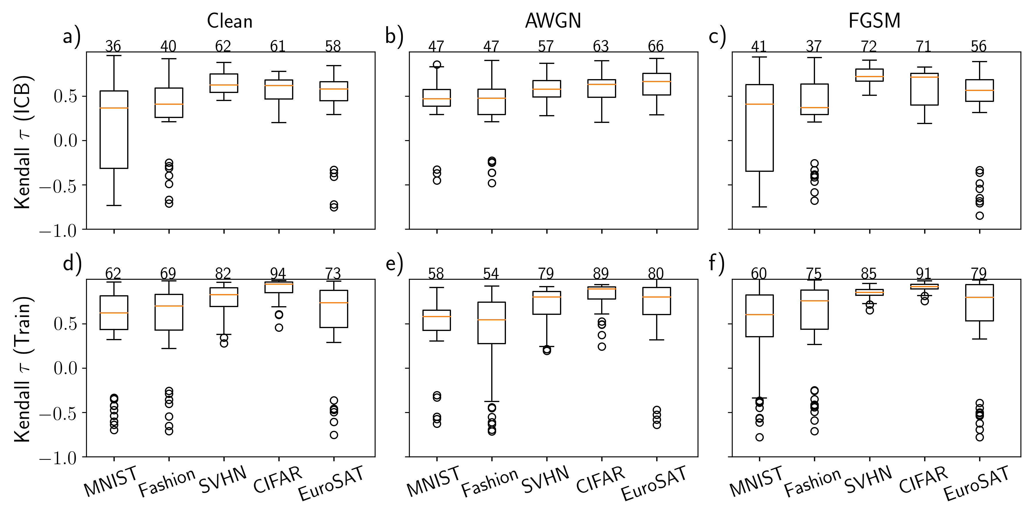
Figure 12: Boxplots show the Kendall $\tau$ ranking between: a,d) Clean, b,e) AWGN, and c,f) FGSM GEs and ICB (top row) compared to a training accuracy baseline (bottom row). We discard $\tau$ values with corresponding $p>0.05$. The median $\tau$ value is annotated above each box and multiplied by 100 for ease of interpretation.

A.5 Advantage of ICB versus MI

To gain further insight into ICB, we examine GEs for a specific CIFAR-10 binary classification task (classes 2 and 5) using three different training set sizes. Plotting GEs with respect to $I(X;Z)$ alone yields a poor overall ranking, whereas ICB effectively aligns trials with different training set sizes (Figure 13).

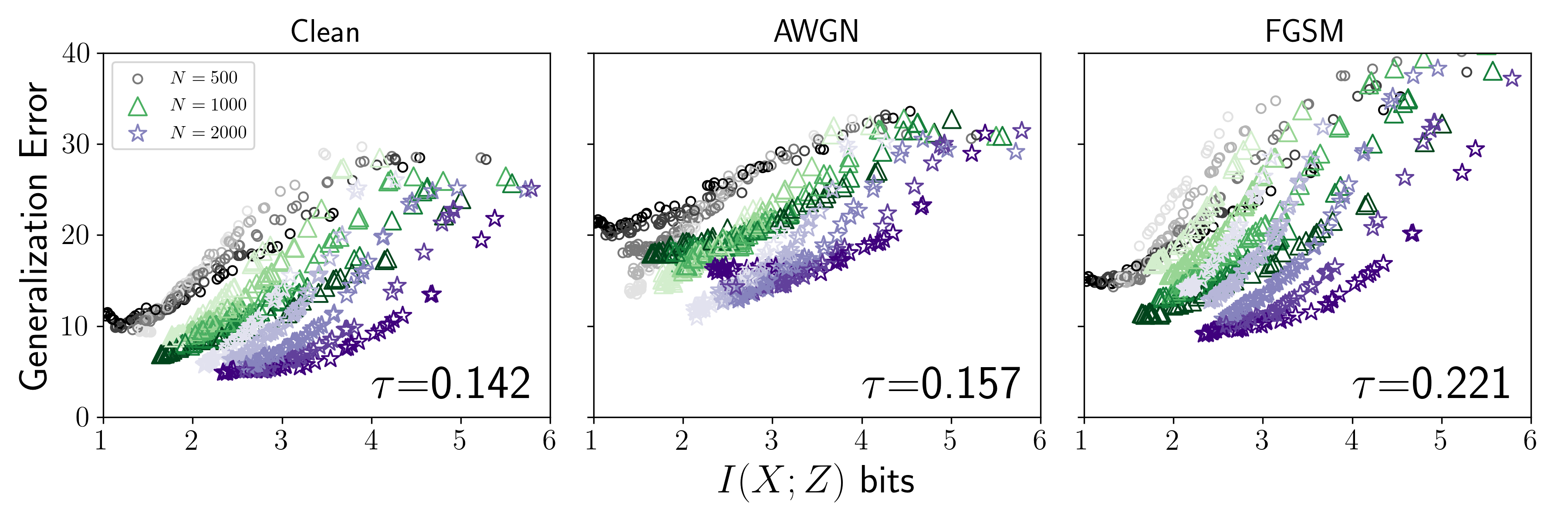
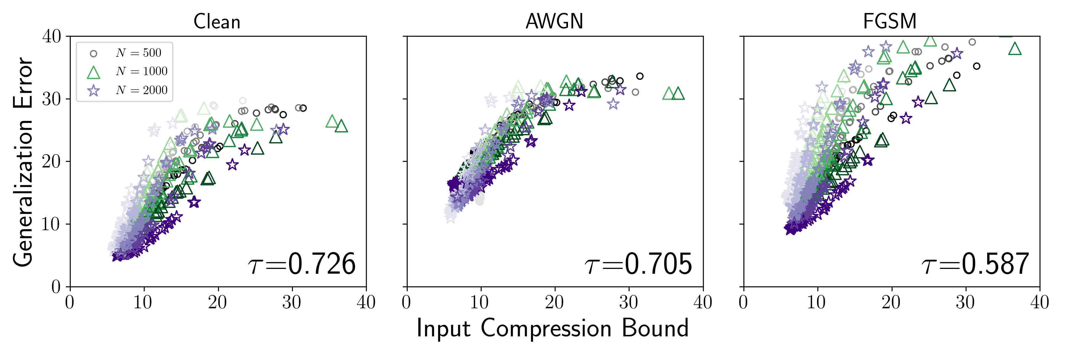
Figure 13: ICB (bottom) ranks GEs better than $I(X;Z)$ alone (top) for different training set sizes. Shown are 750 fully-connected NTK ReLU models trained ($t=\infty$) on a CIFAR-10 binary classification task (classes 2 and 5) using three different training set sizes of $N=\{500,1000,2000\}$ and a test set with $N=2000$. For each training set, 250 meta-parameter combinations are drawn from a uniform random distribution (see §3.2 for details). Model depth is indicated by the colour intensity for each series, where the darkest shade indicates the maximum depth of five (5) layers. Three GE types are evaluated: Clean (standard), AWGN (adversarial), and FGSM (adversarial) are plotted with respect to $I(X;Z)$ (top row) and ICB (bottom row). Plotting GE versus the ICB better aligns results for different sized training sets ($N$) compared to $I(X;Z)$, and yields a better ranking in terms of Kendall-$\tau$.

References

- Ardizzone et al. (2020) Lynton Ardizzone, Radek Mackowiak, Ullrich Köthe, and Carsten Rother. Exact Information Bottleneck with Invertible Neural Networks: Getting the Best of Discriminative and Generative Modeling. arXiv:2001.06448 [cs, stat], 2020.
- Athalye et al. (2018) Anish Athalye, Nicholas Carlini, and David Wagner. Obfuscated Gradients Give a False Sense of Security: Circumventing Defenses to Adversarial Examples. In International Conference on Machine Learning, pp. 274–283, 2018.
- Bachmann et al. (2021) Gregor Bachmann, Thomas Hofmann, and Aurelien Lucchi. Generalization Through the Lens of Leave-One-Out Error. 2021. doi: 10.48550/arXiv.2203.03443.
- Belkin et al. (2018) Mikhail Belkin, Siyuan Ma, and Soumik Mandal. To Understand Deep Learning We Need to Understand Kernel Learning. In Proceedings of the 35th International Conference on Machine Learning, pp. 541–549. PMLR, 2018.
- Belkin et al. (2019) Mikhail Belkin, Daniel Hsu, Siyuan Ma, and Soumik Mandal. Reconciling modern machine-learning practice and the classical bias–variance trade-off. Proceedings of the National Academy of Sciences, 116(32):15849–15854, 2019. doi: 10.1073/pnas.1903070116.
- Bell & Sejnowski (1995) Anthony J. Bell and Terrence J. Sejnowski. An information-maximization approach to blind separation and blind deconvolution. Neural Comput., 7(6):1129–1159, 1995.
- Biggio & Roli (2018) Battista Biggio and Fabio Roli. Wild patterns: Ten years after the rise of adversarial machine learning. In Proceedings of the 2018 ACM SIGSAC Conference on Computer and Communications Security, CCS ’18, pp. 2154–2156, New York, NY, USA, 2018. Association for Computing Machinery. ISBN 978-1-4503-5693-0. doi: 10.1145/3243734.3264418.
- Canatar et al. (2021a) Abdulkadir Canatar, Blake Bordelon, and Cengiz Pehlevan. Out-of-distribution generalization in kernel regression. Advances in neural information processing systems, 34:12600–12612, 2021a. doi: 10.48550/arXiv.2106.02261.
- Canatar et al. (2021b) Abdulkadir Canatar, Blake Bordelon, and Cengiz Pehlevan. Spectral Bias and Task-Model Alignment Explain Generalization in Kernel Regression and Infinitely Wide Neural Networks. Nature Communications, 12(1):2914, 2021b. ISSN 2041-1723. doi: 10.1038/s41467-021-23103-1.
- Carlini et al. (2019) Nicholas Carlini, Anish Athalye, Nicolas Papernot, Wieland Brendel, Jonas Rauber, Dimitris Tsipras, Ian Goodfellow, Aleksander Madry, and Alexey Kurakin. On evaluating adversarial robustness. arXiv preprint arXiv:1902.06705, 2019.
- Chechik et al. (2005) Gal Chechik, Amir Globerson, Naftali Tishby, and Yair Weiss. Information Bottleneck for Gaussian Variables. Journal of Machine Learning Research, 6(Jan):165–188, 2005.
- Chelombiev et al. (2019) Ivan Chelombiev, Conor Houghton, and Cian O’Donnell. Adaptive Estimators Show Information Compression in Deep Neural Networks. In International Conference on Learning Representations, 2019.
- Cover & Thomas (1991) Thomas M Cover and Joy A Thomas. Elements of Information Theory. John Wiley & Sons, Inc., New York, 1991.
- Dziugaite & Roy (2017) Gintare Karolina Dziugaite and Daniel M. Roy. Computing Nonvacuous Generalization Bounds for Deep (Stochastic) Neural Networks with Many More Parameters than Training Data. In Uncertainty in Artificial Intelligence (UAI), 2017.
- Fawzi et al. (2016) Alhussein Fawzi, Seyed-Mohsen Moosavi-Dezfooli, and Pascal Frossard. Robustness of classifiers: From adversarial to random noise. In Advances in Neural Information Processing Systems, volume 29. Curran Associates, Inc., 2016.
- Gabrié et al. (2018) Marylou Gabrié, Andre Manoel, Clément Luneau, jean barbier, Nicolas Macris, Florent Krzakala, and Lenka Zdeborová. Entropy and mutual information in models of deep neural networks. In Advances in Neural Information Processing Systems 31, pp. 1821–1831. Curran Associates, Inc., 2018.
- Gilmer et al. (2019) Justin Gilmer, Nicolas Ford, Nicholas Carlini, and Ekin Cubuk. Adversarial Examples Are a Natural Consequence of Test Error in Noise. In Proceedings of the 36th International Conference on Machine Learning, pp. 2280–2289. PMLR, 2019.
- Goldfeld et al. (2019) Ziv Goldfeld, Ewout Van Den Berg, Kristjan Greenewald, Igor Melnyk, Nam Nguyen, Brian Kingsbury, and Yury Polyanskiy. Estimating Information Flow in Deep Neural Networks. In Proceedings of the 36th International Conference on Machine Learning, volume 97 of Proceedings of Machine Learning Research, pp. 2299–2308. PMLR, 2019.
- Goodfellow et al. (2015) Ian. J. Goodfellow, Jonathon. Shlens, and Christian. Szegedy. Explaining and Harnessing Adversarial Examples. In International Conference on Learning Representations, 2015.
- Helber et al. (2018) Patrick Helber, Benjamin Bischke, Andreas Dengel, and Damian Borth. Introducing EuroSAT: A novel dataset and deep learning benchmark for land use and land cover classification. In IGARSS 2018-2018 IEEE International Geoscience and Remote Sensing Symposium, pp. 204–207, 2018.
- Helber et al. (2019) Patrick Helber, Benjamin Bischke, Andreas Dengel, and Damian Borth. Eurosat: A novel dataset and deep learning benchmark for land use and land cover classification. IEEE Journal of Selected Topics in Applied Earth Observations and Remote Sensing, 2019.
- Jacobsen et al. (2018) Jörn-Henrik Jacobsen, Arnold W. M. Smeulders, and Edouard Oyallon. I-RevNet: Deep Invertible Networks. In International Conference on Learning Representations, 2018.
- Jacot et al. (2018) Arthur Jacot, Franck Gabriel, and Clement Hongler. Neural tangent kernel: Convergence and generalization in neural networks. In Advances in Neural Information Processing Systems 31, pp. 8571–8580. Curran Associates, Inc., 2018.
- Jiang* et al. (2019) Yiding Jiang*, Behnam Neyshabur*, Hossein Mobahi, Dilip Krishnan, and Samy Bengio. Fantastic Generalization Measures and Where to Find Them. In International Conference on Learning Representations, 2019.
- Jiang et al. (2021) Yiding Jiang, Parth Natekar, Manik Sharma, Sumukh K. Aithal, Dhruva Kashyap, Natarajan Subramanyam, Carlos Lassance, Daniel M. Roy, Gintare Karolina Dziugaite, Suriya Gunasekar, Isabelle Guyon, Pierre Foret, Scott Yak, Hossein Mobahi, Behnam Neyshabur, and Samy Bengio. Methods and Analysis of The First Competition in Predicting Generalization of Deep Learning. In Proceedings of the NeurIPS 2020 Competition and Demonstration Track, pp. 170–190. PMLR, 2021.
- Krizhevsky (2009) Alex Krizhevsky. Learning multiple layers of features from tiny images. Technical report, 2009.
- Lachenbruch (1967) P. A. Lachenbruch. An almost unbiased method of obtaining confidence intervals for the probability of misclassification in discriminant analysis. Biometrics, 23(4):639–645, 1967. ISSN 0006-341X.
- LeCun & Cortes (1998) Yann LeCun and Corinna Cortes. The MNIST Database of Handwritten Digits. http://yann.lecun.com/exdb/mnist/, 1998.
- Lee et al. (2019) Jaehoon Lee, Lechao Xiao, Samuel Schoenholz, Yasaman Bahri, Roman Novak, Jascha Sohl-Dickstein, and Jeffrey Pennington. Wide neural networks of any depth evolve as linear models under gradient descent. In Advances in Neural Information Processing Systems 32, pp. 8570–8581. Curran Associates, Inc., 2019.
- Lee et al. (2020) Jaehoon Lee, Samuel Schoenholz, Jeffrey Pennington, Ben Adlam, Lechao Xiao, Roman Novak, and Jascha Sohl-Dickstein. Finite versus infinite neural networks: An empirical study. In Advances in Neural Information Processing Systems, volume 33, pp. 15156–15172. Curran Associates, Inc., 2020.
- Li et al. (2021) Mufan Bill Li, Mihai Nica, and Daniel M. Roy. The Future is Log-Gaussian: ResNets and Their Infinite-Depth-and-Width Limit at Initialization. In Advances in Neural Information Processing Systems, 2021.
- Netzer et al. (2011) Yuval Netzer, Tao Wang, Adam Coates, Alessandro Bissacco, Bo Wu, and Andrew Y Ng. Reading Digits in Natural Images with Unsupervised Feature Learning. In NIPS Workshop on Deep Learning and Unsupervised Feature Learning, 2011.
- Neyshabur et al. (2015) Behnam Neyshabur, Ryota Tomioka, and Nathan Srebro. Norm-Based Capacity Control in Neural Networks. In Proceedings of The 28th Conference on Learning Theory, 2015.
- Novak et al. (2020) Roman Novak, Lechao Xiao, Jiri Hron, Jaehoon Lee, Alexander A. Alemi, Jascha Sohl-Dickstein, and Samuel S. Schoenholz. Neural tangents: Fast and easy infinite neural networks in python. In International Conference on Learning Representations, 2020.
- Paninski (2003) Liam Paninski. Estimation of Entropy and Mutual Information. In Neural Computation, volume 15, pp. 1191–1253. 2003.
- Poole et al. (2019) Ben Poole, Sherjil Ozair, Aaron Van Den Oord, Alex Alemi, and George Tucker. On Variational Bounds of Mutual Information. In Proceedings of the 36th International Conference on Machine Learning, volume 97 of Proceedings of Machine Learning Research, pp. 5171–5180. PMLR, 2019.
- Saxe et al. (2018) Andrew Michael Saxe, Yamini Bansal, Joel Dapello, Madhu Advani, Artemy Kolchinsky, Brendan Daniel Tracey, and David Daniel Cox. On the Information Bottleneck Theory of Deep Learning. In International Conference on Learning Representations, 2018.
- Shwartz-Ziv (2022) Ravid Shwartz-Ziv. Information Flow in Deep Neural Networks. 2022. doi: 10.48550/arXiv.2202.06749.
- Shwartz-Ziv & Alemi (2020) Ravid Shwartz-Ziv and Alexander A Alemi. Information in infinite ensembles of infinitely-wide neural networks. In Proceedings of the 2nd Symposium on Advances in Approximate Bayesian Inference, volume 118 of Proceedings of Machine Learning Research, pp. 1–17. PMLR, 2020.
- Shwartz-Ziv et al. (2019) Ravid Shwartz-Ziv, Amichai Painsky, and Naftali Tishby. Representation Compression and Generalization in Deep Neural Networks. OpenReview, 2019.
- Strouse & Schwab (2016) D. J. Strouse and David J. Schwab. The deterministic information bottleneck. In Uncertainty in Artificial Intelligence (UAI), 2016.
- Szegedy et al. (2014) Christian Szegedy, Wojciech Zaremba, Ilya Sutskever, Joan Bruna, Dumitru Erhan, Ian Goodfellow, and Rob Fergus. Intriguing properties of neural networks. In International Conference on Learning Representations, 2014.
- Tishby (2017) Naftali Tishby. Information Theory of Deep Learning, 2017. URL https://youtu.be/bLqJHjXihK8?t=1051.
- Tsipras et al. (2019) Dimitris Tsipras, Shibani Santurkar, Logan Engstrom, Alexander Turner, and Aleksander Madry. Robustness May Be at Odds with Accuracy. In International Conference on Learning Representations, 2019.
- van den Oord et al. (2018) Aaron van den Oord, Yazhe Li, and Oriol Vinyals. Representation Learning with Contrastive Predictive Coding. 2018. doi: 10.48550/arXiv.1807.03748.
- Xiao et al. (2017) Han Xiao, Kashif Rasul, and Roland Vollgraf. Fashion-MNIST: A novel image dataset for benchmarking machine learning algorithms, 2017.
- Zhang et al. (2017) Chiyuan Zhang, Samy Bengio, Moritz Hardt, Benjamin Recht, and Oriol Vinyals. Understanding deep learning requires rethinking generalization. In International Conference on Learning Representations, 2017.
- Zhang et al. (2021) Chiyuan Zhang, Samy Bengio, Moritz Hardt, Benjamin Recht, and Oriol Vinyals. Understanding deep learning (still) requires rethinking generalization. Communications of the ACM, 64(3):107–115, 2021. ISSN 0001-0782. doi: 10.1145/3446776.
- Zhou et al. (2019) Wenda Zhou, Victor Veitch, Morgane Austern, Ryan P. Adams, and Peter Orbanz. Non-vacuous Generalization Bounds at the ImageNet Scale: A PAC-Bayesian Compression Approach. In International Conference on Learning Representations, 2019.