Riemannian Stochastic Gradient Method for Nested Composition Optimization

Abstract

This work considers optimization of composition of functions in a nested form over Riemannian manifolds where each function contains an expectation. This type of problems is gaining popularity in applications such as policy evaluation in reinforcement learning or model customization in meta-learning. The standard Riemannian stochastic gradient methods for non-compositional optimization cannot be directly applied as stochastic approximation of inner functions create bias in the gradients of the outer functions. For two-level composition optimization, we present a Riemannian Stochastic Composition Gradient Descent (R-SCGD) method that finds an approximate stationary point, with expected squared Riemannian gradient smaller than $\epsilon$, in $\mathcal{O}(\epsilon^{-2})$ calls to the stochastic gradient oracle of the outer function and stochastic function and gradient oracles of the inner function. Furthermore, we generalize the R-SCGD algorithms for problems with multi-level nested compositional structures, with the same complexity of $\mathcal{O}(\epsilon^{-2})$ for the first-order stochastic oracle. Finally, the performance of the R-SCGD method is numerically evaluated over a policy evaluation problem in reinforcement learning.

Keywords: Manifold optimization, Riemannian optimization, Stochastic compositional optimization.

1 Introduction

We consider optimizing nested stochastic compositional functions over Riemannian manifolds. The two-level compositional optimization problem has the form

$$\min_{\mathbf{x}\in\mathcal{M}}F(\mathbf{x})=\mathbb{E}_{\xi}[f_{\xi}(\mathbb{E}_{\phi}[g_{\phi}(\mathbf{x})])]$$ (1)

where $g_{\phi}:\mathcal{M}\to\mathcal{N}$ is a smooth map, $\mathcal{M}$ and $\mathcal{N}\subseteq\mathcal{E}$ are Riemannian manifolds, $\mathcal{E}$ is a Euclidean space, $f_{\xi}:\mathcal{E}\to\mathbb{R}$ is a continuously differentiable function, and $\xi$ and $\phi$ are independent random variables (Absil et al. 2009). With a slight abuse of notation, we denote $\mathbb{E}_{\xi}[f_{\xi}(\cdot)]$, $\mathbb{E}_{\phi}[g_{\phi}(\cdot)]$ by $f(\cdot)$ and $g(\cdot)$, respectively. We assume throughout the paper that there exists at least one global optimal solution $\mathbf{x}^{*}\in\mathcal{M}$ to problem (1). We do not require either the outer function $f_{\xi}$ or the inner function $g_{\phi}$ to be (geodesically) convex or monotone. As a result, the composition problem cannot be reformulated into a saddle point problem in general (Zhang and Lan 2020). The Riemannian stochastic gradient method (Bonnabel 2013) cannot be applied to solve (1) since the stochastic gradient $\nabla f_{\xi}$ evaluated at the stochastic function value $g_{\phi}$ does not result in an unbiased estimate of $\nabla f(g(x))$ which then results in a biased estimate of $\nabla F(\mathbf{x})$ (Robbins and Monro 1951). Hence, a special algorithmic setup is required to tackle this type of problem.

The stochastic compositional optimization finds applications in reinforcement learning for policy evaluation, meta-learning, stochastic minimax problems, dynamic programming and risk-averse problems (Ben-Tal and Nemirovski 2002, Bertsekas 2012, Goodfellow et al. 2016, Finn et al. 2017, Sutton and Barto 2018). The Riemannian manifold constraint arises due to 1) recent reformulation of some nonconvex problems as geodesically convex problems over manifolds (Zhang and Sra 2016, Vishnoi 2018), 2) significant computational or performance gains in introducing manifolds constraints in some applications, e.g., training deep neural networks by enforcing hidden-layer weight matrices to belong to Stiefel manifolds (Arjovsky et al. 2016, Wisdom et al. 2016, Bansal et al. 2018, Xie et al. 2017), 3) new optimization problems that intrinsically involve manifold constraints (Absil and Hosseini 2019, Hu et al. 2020, Hosseini and Sra 2020, Vandereycken 2013).

Below, we present a policy evaluation problem in reinforcement learning which has two-level nested compositional form over Riemannian manifolds as (1).

Motivating example.

In reinforcement learning, finding the value function of a given policy is often referred to as policy evaluation problem (Dann et al. 2014, Wang et al. 2017, Sutton and Barto 2018). Suppose there are $S$ states with the state variable $s\in\mathbb{R}^{d}$ and denote the policy of interest by $\pi$. Let $V^{\pi}\in\mathbb{R}^{S}$ denote the value function, where $V^{\pi}(s)$ represents the value of state $s$ under policy $\pi$. The Bellman equation that should be satisfied by the optimal policy is

$$V^{\pi}(s)=\mathbb{E}[r_{s,s^{\prime}}+\rho V^{\pi}(s^{\prime})|s],\ \ \forall s,s^{\prime}\in\{1,...,S\},$$ (2)

where $\rho<1$ is a discount factor, $r_{s,s^{\prime}}$ is the reward of transition from state $s$ to state $s^{\prime}$, and the expectation is taken over all possible future states $s^{\prime}$ conditioned on current state $s$ and the policy $\pi$. In the blackbox simulation environment, the transition and reward matrices are unknown, but can be sampled. Furthermore, large number of states $S$ makes solving the Bellman equation directly impractical. Therefore, we model the value function with Gaussian basis functions (see Bishop (2006)) and consider an iterative procedure to estimate the parameters. In particular, we assume that $V^{\pi}(s)\approx\sum_{i=1}^{D}w_{i}N(s;\mu_{i},\Sigma_{i})$, where $D\ll S$. We denote $\sum_{i=1}^{D}w_{i}N(s;\mu_{i},\Sigma_{i})$ by $\varphi(s;\Lambda)$, where $\Lambda\triangleq\{\{w_{i}\},\{\mu_{i}\},\{\Sigma_{i}\}\}_{i=1}^{D}$ is the set of all parameters.

The policy evaluation problem is formulated as

$$\min_{\Lambda}\sum_{s}[\varphi(s;\Lambda)-\sum_{s^{\prime}}\mathbb{E}[\hat{P}_{s,s^{\prime}}](\mathbb{E}[\hat{r}_{s,s^{\prime}}]+\rho\varphi(s^{\prime};\Lambda))]^{2}$$ (3)

where the optimization variables are on the product of the Euclidean spaces and the manifolds of positive definite matrices. Problem (3) is an instance of (1) with $f(\cdot)=\|\cdot\|^{2}$ and function $g$ defined as $g:\mathbb{R}^{D}\times\mathbb{R}^{D\times d}\times\mathcal{M}^{D}\longrightarrow\mathbb{R}^{S},\{\{w_{i}\},\{\mu_{i}\},\{\Sigma_{i}\}\}_{i=1}^{D}\longmapsto(g_{1},...,g_{S})$,

$$g_{s}\triangleq\varphi(s;\Lambda)-\sum_{s^{\prime}}\mathbb{E}[\hat{P}_{s,s^{\prime}}](\mathbb{E}[\hat{r}_{s,s^{\prime}}]+\rho\varphi(s^{\prime};\Lambda)).$$ (4)

1.1 Related work

This work stems from two different lines of research: 1. Manifold optimization, 2. Stochastic compositional optimization in Euclidean setting which are briefly reviewed below.

Manifold optimization.

The stochastic gradient descent (SGD) method over manifolds was first studied in Bonnabel (2013) which proved Riemannian SGD converges to a critical point of the problem. Under geodesic convexity, Zhang and Sra (2016) developed the first global complexity of first-order methods (in general) and established $\mathcal{O}(1/\epsilon^{2})$ complexity to attain an $\epsilon$-optimal solution, i.e., $f(x^{k})-f^{*}\leq\epsilon$, for Riemannian SGD. In the Euclidean setting, many variance reduction techniques have been proposed to improve the sample complexity of SGD (Roux et al. 2012, Johnson and Zhang 2013, Xiao and Zhang 2014, Defazio et al. 2014, Reddi et al. 2016, Allen-Zhu and Hazan 2016). As a generalization of Johnson and Zhang (2013), the Riemannian stochastic variance-reduced gradient descent (R-SVRG) method was developed in Zhang et al. (2016), establishing the linear rate for geodesically strongly convex functions. An extension of Riemannian SVRG with computationally more efficient retraction and vector transport was developed in Sato et al. (2019). In Tripuraneni et al. (2018), authors adapted the Polyak-Ruppert iterate averaging over Riemannian manifolds (Ruppert 1988, Polyak 1990) reaching $\mathcal{O}(1/k)$ rate. The Riemannian version of the stochastic recursive gradient method (Nguyen et al. 2017) was proposed in Kasai et al. (2018). Kasai et al. (2019) proposed the adaptive gradient method with the convergence rate of $\mathcal{O}(\log(k)/\sqrt{k})$.

Besides the stochastic gradient methods, numerous deterministic algorithms for Euclidean unconstrained optimization (Nocedal and Wright 2006, Ruszczynski 2011) have also been generalized to Riemannian settings (Absil et al. 2009, Udriste 2013, Boumal 2020) - see, for instance, gradient descent (Zhang and Sra 2016), the Nesterov’s accelerated method (Liu et al. 2017, Zhang and Sra 2018, Ahn and Sra 2020, Alimisis et al. 2020), proximal gradient method (Huang and Wei 2021), Frank-Wolfe method (Weber and Sra 2019), nonlinear conjugate gradient method (Smith 1994, Sato and Iwai 2015), BFGS (Ring and Wirth 2012), Newton’s method (Adler et al. 2002, Kasai et al. 2018), trust-region method (Absil et al. 2007) and cubic regularized method (Zhang and Zhang 2018, Agarwal et al. 2018, Zhang and Tajbakhsh 2020).

Stochastic compositional optimization.

The stochastic compositional optimization is closely related to the classical SGD and stochastic approximation (SA) methods (Robbins and Monro 1951, Kiefer and Wolfowitz 1952, Kushner and Yin 2003). When the outer function $f$ is linear, the problem reduces to the standard stochastic non-compositional setting which has been extensively studied. While the problem is indeed compositional with two expected-value functions, Ermoliev (1976) applied a simple two-timescale SA scheme, showing its convergence under basic assumptions.

The first nonasymptotic analysis for the stochastic compositional optimization appeared in Wang et al. (2017), which uses two sequences of stepsizes in two different timescales: a slower one $\alpha_{k}$ for updating the optimization variable $\mathbf{x}$ and a faster one $\beta_{k}$ for tracking the value of inner function. Their analysis requires $\alpha_{k}/\beta_{k}\to 0$ as $k\to\infty$. For problems with smooth and convex composition objective, their algorithm converge at a rate of $\mathcal{O}(k^{-2/7})$, and with the rate of $\mathcal{O}(k^{-4/5})$ in the strongly convex case, where $k$ represents the number of queries to the stochastic first-order oracles. The first finite-sample error bound is improved in Wang et al. (2016) to $\mathcal{O}(k^{-4/9})$ for convex and nonconvex settings. While most methods rely on the two-timescale stepsizes, the single timescale algorithm was recently developed in Ghadimi et al. (2020), achieving the sample complexity of $\mathcal{O}(1/\epsilon^{2})$ to find an $\epsilon$-approximate stationary point. Furthermore, Chen et al. (2021) proposed a single-loop loop algorithm, without any need for accuracy-dependent stepsize or increasing batch size, that can achieve the sample complexity of $\mathcal{O}(1/\epsilon^{2})$ as in Chen et al. (2021) (or classic SGD for non-compositional problems).

In addition to the general stochastic optimization, the special setting with finite-sum structure recently gained popularity. The variants of the algorithm in Wang et al. (2017) for finite-sum setting have been proposed in Lian et al. (2017), Blanchet et al. (2017), Devraj and Chen (2019), Lin et al. (2018), Xu and Xu (2021). Furthermore, the stochastic compositional problem with certain nonsmooth component was investigated in Huo et al. (2018), Zhang and Xiao (2019b, a). A key feature of these works is involving variance reduction techniques, which helps to achieve better performance for the finite-sum stochastic compositional problems. As these methods usually require increasing batch size, it is not possible to directly use them for general stochastic compositional problems.

1.2 Contributions

The main contributions of this paper are as follows: 1) The paper proposes algorithms to optimize stochastic compositional functions over Riemannian manifolds for both bi-level and multi-level settings. To our best knowledge, this is the first work opening the discussion for future works. The algorithms are motivated by the Riemannian extension of the ODE gradient flow presented in Chen et al. (2021) for the unconstrained Euclidean setting. 2) Under regular Riemannian Lipschitz continuity assumptions, the algorithm does not require embedding assumption of $\mathcal{M}$ in a vector space. Furthermore, it is independent of Riemannian operations, e.g., exponential map or parallel translate, over the manifolds resulting from the mappings of $\mathcal{M}$ by the inner function(s), e.g., by $g_{\phi}$ in (1). 3) We provide the sample complexity of the proposed algorithms obtaining $\mathcal{O}(1/\epsilon^{2})$ to obtain $\epsilon$-approximate stationary solution, i.e., $\|\text{grad}f(x)\|^{2}\leq\epsilon$, which is the same rate as Riemannian SGD for stochastic non-compositional problems (Hosseini and Sra 2020) or the algorithms in Chen et al. (2021) and Ghadimi et al. (2020) for Euclidean compositional problems. 4) We empirically verify the effectiveness of the proposed algorithm for two-level compositional problems in the policy evaluation problem discussed in section 1.

1.3 Preliminaries

A Riemannnian manifold $(\mathcal{M},g)$ is a real smooth manifold $\mathcal{M}$ equipped with a Riemannain metric $g$. The metric $g$ induces an inner product structure in each tangent space $T_{\mathbf{x}}\mathcal{M}$ associated with point $\mathbf{x}\in\mathcal{M}$. We denote the inner product of $\mathbf{u},\mathbf{v}\in T_{\mathbf{x}}\mathcal{M}$ as $\left\langle\mathbf{u},\mathbf{v}\right\rangle_{x}$, and the norm of $\mathbf{u}$ is defined as $\|\mathbf{u}\|=\sqrt{\left\langle\mathbf{u},\mathbf{u}\right\rangle_{x}}$. Given a smooth real-valued function $f$ on a Riemannian manifold $\mathcal{M}$, Riemannian gradient of $f$ at $\mathbf{x}$ is denoted by $\text{grad}f(\mathbf{x})$. We use $\nabla f$ to denote the gradient (or Jacobian) of a scalar (or vector) valued function $f$ in the Euclidean sense.

Definition 1.

Given manifolds $\mathcal{M}$ and $\mathcal{M}^{\prime}$, the differential of a smooth map $F:\mathcal{M}\to\mathcal{M}^{\prime}$ at $\mathbf{x}$ is a linear operator $DF(\mathbf{x}):\mathcal{T}_{\mathbf{x}}\mathcal{M}\to\mathcal{T}_{F(\mathbf{x})}\mathcal{M}^{\prime}$ defined by:

$$DF(\mathbf{x})[v]=[t\mapsto F(c(t))],$$ (5)

where $c$ is a smooth curve on $\mathcal{M}$ passing through $\mathbf{x}$ at $t=0$ such that $v=[c]$. In particular, when $\mathcal{M}^{\prime}$ is an embedded submanifold of a linear space $\mathcal{E}$, identifying the tangent spaces of $\mathcal{M}^{\prime}$ to subspaces of $\mathcal{E}$ and with $v=[c]$ a tangent vector at $\mathbf{x}\in\mathcal{M}$, we write

$$DF(\mathbf{x})[v]=(F\circ c)^{\prime}(0),$$ (6)

where $F\circ c$ is seen as a map into $\mathcal{E}$.

Definition 2 (Riemannian gradient).

Let $f:\mathcal{M}\rightarrow\mathbb{R}$ be a smooth function on a Riemannian manifold $\mathcal{M}$. The Riemannian gradient of $f$ is the vector field $\text{grad}f$ on $\mathcal{M}$ that $\forall\mathbf{x}\in\mathcal{M},\forall v\in T_{\mathbf{x}}\mathcal{M}$ satisfies

$$Df(\mathbf{x})[v]=\left\langle v,\text{grad}f(\mathbf{x})\right\rangle_{\mathbf{x}},$$ (7)

where $Df(\mathbf{x})$ is the differential of $f$ at $\mathbf{x}\in\mathcal{M}$.

Definition 3 (Adjoint of an operator).

Let $\mathcal{E}$ and $\mathcal{E}^{\prime}$ be two Euclidean spaces, with inner products $\left\langle\cdot,\cdot\right\rangle_{a}$ and $\left\langle\cdot,\cdot\right\rangle_{b}$ respectively. Let $\mathcal{A}:\mathcal{E}\mapsto\mathcal{E}^{\prime}$ be a linear operator. The adjoint of $\mathcal{A}$ is a linear operator $\mathcal{A}^{*}:\mathcal{E}^{\prime}\mapsto\mathcal{E}$ and we have

$$\forall\mathbf{u}\in\mathcal{E},\mathbf{v}\in\mathcal{E}^{\prime},\ \ \left\langle\mathcal{A}(\mathbf{u}),\mathbf{v}\right\rangle_{b}=\left\langle\mathbf{u},\mathcal{A}^{*}(\mathbf{v})\right\rangle_{a}.$$ (8)

2 Two-level Riemannian composition

We first characterize the Riemannian gradient of the composite function $F(\mathbf{x})$

$$DF(\mathbf{x})[v] =Df(g(\mathbf{x}))[Dg(\mathbf{x})[v]]$$

$$=\left\langle\text{Proj}_{g(\mathbf{x})}\nabla f(g(\mathbf{x})),Dg(\mathbf{x})[v]\right\rangle$$

$$=\left\langle(Dg(\mathbf{x}))^{*}(\text{Proj}_{g(\mathbf{x})}\nabla f(g(\mathbf{x}))),v\right\rangle_{\mathbf{x}}$$

where $\text{Proj}_{g(\mathbf{x})}$ is the orthogonal projection onto $T_{g(\mathbf{x})}\mathcal{N}$ follows from the embedding assumption of $\mathcal{N}$ in the Euclidean space. According to Definition 2, the Riemannian gradient of $F(\mathbf{x})$, denoted by $\text{grad}F(\mathbf{x})$, is $(Dg(\mathbf{x}))^{*}(\text{Proj}_{g(\mathbf{x})}\nabla f(g(\mathbf{x})))$.

Following the standard SGD methodology applied on manifold optimization (Robbins and Monro 1951, Bonnabel 2013, Zhang et al. 2016, Zhang and Sra 2016, Hosseini and Sra 2020), a promising update is

$$\mathbf{x}^{k+1}=\text{Exp}_{\mathbf{x}^{k}}(-\alpha(Dg_{\phi^{k}}(\mathbf{x}^{k}))^{*}(\text{Proj}_{g(\mathbf{x}^{k})}\nabla f_{\xi^{k}}(g(\mathbf{x}^{k})))),$$ (9)

where $\phi^{k}$ and $\xi^{k}$ are samples drawn at iteration $k$. Note that $Dg_{\phi^{k}}(\mathbf{x}^{k}))^{*}(\text{Proj}_{g(\mathbf{x}^{k})}\nabla f_{\xi^{k}}(g(\mathbf{x}^{k}))$ is an unbiased estimator of $\text{grad }F(\mathbf{x})$ but the exact evaluation of $g(\mathbf{x}^{k})$, i.e. $\mathbb{E}_{\phi}[g_{\phi}(\mathbf{x}^{k})]$, is generally not attainable. Furthermore, the stochastic gradient is not unbiased if one replaces $g(\mathbf{x}^{k})$ by its stochastic estimate $g_{\phi^{k}}(\mathbf{x}^{k})$. Therefore, the stochastic gradient method cannot be directly applied.

2.1 Algorithm development motivated by ODE analysis

Below, we provide the intuition behind our algorithmic design based on the ODE gradient flow which carefully extends the analysis in Chen et al. (2021) to the Riemannian setting.

Let $t$ be time in this subsection. Consider the following ODE

$$\dot{\mathbf{x}}(t)=-\alpha(Dg(\mathbf{x}))^{*}\text{Proj}_{g(\mathbf{x})}\nabla f(\mathbf{y}(t)),$$ (10)

for some $\alpha>0$. If we set $\mathbf{y}(t)=g(\boldsymbol{\mathbf{x}}(t))$, then we have

$$\frac{d}{dt}f(g(\boldsymbol{\mathbf{x}}(t)))=\left\langle(Dg(\mathbf{x}))^{*}\text{Proj}_{g(\mathbf{x})}\nabla f(g(\boldsymbol{\mathbf{x}}(t))),\dot{\boldsymbol{\mathbf{x}}}(t)\right\rangle_{\boldsymbol{\mathbf{x}}(t)}=-\frac{1}{\alpha}\|\dot{\boldsymbol{\mathbf{x}}}(t)\|^{2}_{\boldsymbol{\mathbf{x}}(t)}\leq 0.$$

In this case, (10) describes a gradient flow that monotonically decreases $f(g(\boldsymbol{\mathbf{x}}(t)))$. However, we can not evaluate $g(\boldsymbol{\mathbf{x}}(t))$ exactly. Instead, we can evaluate $\nabla f$ at $\mathbf{y}(t)\approx g(\boldsymbol{\mathbf{x}}(t))$, and the introduced inexactness results in $f(g(\boldsymbol{\mathbf{x}}(t)))$ loosing its monotonicity:

$$\frac{d}{dt}f(g(\boldsymbol{\mathbf{x}}(t))) =-\frac{1}{\alpha}\|\dot{\boldsymbol{\mathbf{x}}}(t)\|^{2}_{\boldsymbol{\mathbf{x}}(t)}+\left\langle(Dg(\mathbf{x}))^{*}\text{Proj}_{g(\mathbf{x})}(\nabla f(g(\boldsymbol{\mathbf{x}}(t)))-\nabla f(\mathbf{y}(t))),\dot{\boldsymbol{\mathbf{x}}}(t)\right\rangle_{\boldsymbol{\mathbf{x}}(t)}$$

$$=-\frac{1}{\alpha}\|\dot{\boldsymbol{\mathbf{x}}}(t)\|^{2}_{\boldsymbol{\mathbf{x}}(t)}+\left\langle\text{Proj}_{g(\mathbf{x})}(\nabla f(g(\boldsymbol{\mathbf{x}}(t)))-\nabla f(\mathbf{y}(t))),Dg(\mathbf{x})[\dot{\boldsymbol{\mathbf{x}}}(t)]\right\rangle_{g(\boldsymbol{\mathbf{x}}(t))}$$

$$\leq-\frac{1}{\alpha}\|\dot{\boldsymbol{\mathbf{x}}}(t)\|^{2}_{\boldsymbol{\mathbf{x}}(t)}+\|Dg(\mathbf{x})[\dot{\boldsymbol{\mathbf{x}}}(t)]\|_{g(\boldsymbol{\mathbf{x}}(t))}\|\text{Proj}_{g(\mathbf{x})}(\nabla f(g(\boldsymbol{\mathbf{x}}(t)))-\nabla f(\mathbf{y}(t)))\|_{g(\boldsymbol{\mathbf{x}}(t))}$$

$$\leq-\frac{1}{\alpha}\|\dot{\boldsymbol{\mathbf{x}}}(t)\|^{2}_{\boldsymbol{\mathbf{x}}(t)}+L_{f}C_{g}\|g(\mathbf{x}(t))-\mathbf{y}(t)\|\cdot\|\dot{\mathbf{x}}(t)\|_{\mathbf{x}(t)}$$

$$\leq-\frac{1}{2\alpha}\|\dot{\boldsymbol{\mathbf{x}}}(t)\|^{2}_{\boldsymbol{\mathbf{x}}(t)}+\frac{\alpha C_{g}^{2}L_{f}^{2}}{2}\|g(\boldsymbol{\mathbf{x}}(t))-\mathbf{y}(t))\|^{2}.$$

This motivates an energy function,

$$V(t)=f(g(\boldsymbol{\mathbf{x}}(t)))+\|g(\boldsymbol{\mathbf{x}}(t))-\mathbf{y}(t)\|^{2}.$$ (11)

We want $V(t)$ to monotonically decrease. By substitution, we have

$$\dot{V}(t) \leq-\frac{1}{2\alpha}\|\dot{\boldsymbol{\mathbf{x}}}(t)\|^{2}_{\boldsymbol{\mathbf{x}}(t)}+\frac{\alpha C_{g}^{2}L_{f}^{2}}{2}\|g(\boldsymbol{\mathbf{x}}(t))-\mathbf{y}(t))\|^{2}+2\left\langle\mathbf{y}(t)-g(\boldsymbol{\mathbf{x}}(t)),\dot{\mathbf{y}}(t)-Dg(\boldsymbol{\mathbf{x}}(t))[\dot{\boldsymbol{\mathbf{x}}}(t)]\right\rangle$$

$$=-\frac{1}{2\alpha}\|\dot{\boldsymbol{\mathbf{x}}}(t)\|^{2}_{\boldsymbol{\mathbf{x}}(t)}-(\beta-\frac{\alpha C_{g}^{2}L_{f}^{2}}{2})\|g(\boldsymbol{\mathbf{x}}(t))-\mathbf{y}(t)\|^{2}+2\langle\mathbf{y}(t)-g(\boldsymbol{\mathbf{x}}(t)),\dot{\mathbf{y}}(t)+\beta(\mathbf{y}(t)-g(\boldsymbol{\mathbf{x}}(t)))$$

$$-Dg(\boldsymbol{\mathbf{x}}(t))[\dot{\boldsymbol{\mathbf{x}}}(t)]\rangle,$$

where $\beta>0$ is a fixed constant. Following the maximum descent principle of $V(t)$, we are motivated to use the following dynamics

$$\dot{\mathbf{y}}(t)=-\beta(\mathbf{y}(t)-g(\boldsymbol{\mathbf{x}}(t)))+Dg(\boldsymbol{\mathbf{x}}(t))[\dot{\boldsymbol{\mathbf{x}}}(t)].$$ (12)

We approximate $Dg(\boldsymbol{\mathbf{x}}(t))[\dot{\boldsymbol{\mathbf{x}}}(t)]$ by the first-order Taylor expansion (Boumal 2020), i.e.,

$$Dg(\boldsymbol{\mathbf{x}}(t))[\dot{\boldsymbol{\mathbf{x}}}(t)]\approx\gamma_{k}(g(\mathbf{x}^{k})-g(\mathbf{x}^{k-1})),$$ (13)

where $k$ is the discrete iteration index, and $\gamma_{k}$ is the weight controlling the approximation.

With the insights gained from (10) and (12), we propose the following stochastic update, which serve as the main components in Algorithm 1.

$$\mathbf{y}^{k+1}= \mathbf{y}^{k}-\beta_{k}(\mathbf{y}^{k}-g_{\phi^{k}}(\mathbf{x}^{k}))+\gamma_{k}(g_{\phi^{k}}(\mathbf{x}^{k})-g_{\phi^{k}}(\mathbf{x}^{k-1})),$$ (14)

$$\mathbf{x}^{k+1}=\text{Exp}_{\mathbf{x}^{k}}(-\alpha(Dg_{\phi^{k}}(\mathbf{x}^{k}))^{*}\text{Proj}_{g_{\phi^{k}}(\mathbf{x}^{k})}\nabla f_{\xi^{k}}(\mathbf{y}^{k+1})).$$ (15)

Algorithm 1 R-SCGD for two-level problem

0:  $\mathbf{x}^{0}$, $\mathbf{y}^{0}$, constant sequences $\{\alpha_{k}\}$, $\{\beta_{k}\}$, $\{\gamma_{k}\}$

1:  for $k=0,...,K-1$ do

2:     Randomly sample $\phi^{k}$ and $\xi^{k}$

3:     Update inner function estimate $\mathbf{y}^{k+1}$ using

$$\mathbf{y}^{k+1}=\mathbf{y}^{k}-\beta_{k}(\mathbf{y}^{k}-g_{\phi^{k}}(\mathbf{x}^{k}))+\gamma_{k}(g_{\phi^{k}}(\mathbf{x}^{k})-g_{\phi^{k}}(\mathbf{x}^{k-1}))$$

4:     Update Riemannian gradient of the composition function as

$$\eta^{k+1}=(Dg_{\phi^{k}}(\mathbf{x}^{k}))^{*}\text{Proj}_{g_{\phi^{k}}(\mathbf{x}^{k})}\nabla f_{\xi^{k}}(\mathbf{y}^{k+1})$$

5:     Update $\mathbf{x}^{k+1}=\text{Exp}_{\mathbf{x}^{k}}(-\alpha_{k}\eta^{k+1})$

6:  end for

2.2 Iteration complexity of the two-level R-SCGD method

With the insights gained from the continuous-time Lyapunov function, our analysis in this section essentially builds on the following discrete-time Lyapunov function

$$\mathcal{V}^{k}:=F(\mathbf{x}^{k})-F(\mathbf{x}^{*})+\|g(\mathbf{x}^{k-1})-\mathbf{y}^{k}\|^{2},$$ (16)

where $\mathbf{x}^{*}$ is (one of) the optimal solution(s) of the problem (1).

Assumption 2.1.

Function $F(\mathbf{x}):\mathcal{M}\to\mathbb{R}$ is geodesically $L_{g}$-smooth, i.e., $\forall(\mathbf{x},\mathbf{s})\in\mathcal{T}$,

$$\|P^{-1}_{s}\text{grad }F(\text{Exp}_{\mathbf{x}}(s))-\text{grad }F(\mathbf{x})\|\leq L_{g}\|s\|,$$ (17)

where $\mathcal{T}\subseteq T\mathcal{M}$ is the domain of Exp and $P_{s}$ denotes parallel transport along $\gamma(t)=\text{Exp}_{\mathbf{x}}(ts)$ from $t=0$ to $t=1$.

Assumption 2.2.

Function $f_{\xi}:\mathcal{E}\to\mathbb{R}$ is $L_{f}$-smooth, i.e., for all $\mathbf{y},\mathbf{y}^{\prime}\in\mathcal{E}$,

$$\|\nabla f_{\xi}(\mathbf{y})-\nabla f_{\xi}(\mathbf{y}^{\prime})\|\leq L_{f}\|\mathbf{y}-\mathbf{y}^{\prime}\|.$$ (18)

Assumption 2.3.

Random sample oracle of function value $g_{\phi}(\mathbf{x})$ is an unbiased estimator of $g(\mathbf{x})$ and has bounded variance, i.e.,

$$\begin{split}\mathbb{E}[g_{\phi}(\mathbf{x})]=g(\mathbf{x}),\\ \mathbb{E}[\|g_{\phi}(\mathbf{x})-g(\mathbf{x})\|^{2}]\leq V_{g}^{2}.\end{split}$$ (19)

Assumption 2.4.

The chain rule holds in expectation, i.e.

$$\mathbb{E}[(Dg_{\phi}(\mathbf{x}))^{*}\text{Proj}_{g_{\phi}(\mathbf{x})}\nabla f_{\xi}(g(\mathbf{x}))]=(Dg(\mathbf{x}))^{*}\text{Proj}_{g(\mathbf{x})}\nabla f(g(\mathbf{x})).$$

Remark 2.1.

If the random sample oracle of derivatives (gradients) satisfies

$$\begin{split}\mathbb{E}[Dg_{\phi}(\mathbf{x})[\eta]]=Dg(\mathbf{x})[\eta],\\ \mathbb{E}[\nabla f_{\xi}(\mathbf{x})]=\nabla f(\mathbf{x}),\end{split}$$ (20)

and with the independence between $\phi$ and $\xi$, Assumption 2.4 holds. See lemma below.

Lemma 2.1.

If the random sample oracle for derivatives (gradients) satisfies

$$\mathbb{E}[Dg_{\phi}(\mathbf{x})[\eta]]=Dg(\mathbf{x})[\eta],\text{and }\mathbb{E}[\nabla f_{\xi}(\mathbf{x})]=\nabla f(\mathbf{x}),$$ (21)

and random variable $\phi$ is independent of $\xi$, then

$$\mathbb{E}[(Dg_{\phi}(\mathbf{x}))^{*}\text{Proj}_{g_{\phi}(\mathbf{x})}\nabla f_{\xi}(g(\mathbf{x}))]=(Dg(\mathbf{x}))^{*}\text{Proj}_{g(\mathbf{x})}\nabla f(g(\mathbf{x})).$$ (22)

Assumption 2.5.

The stochastic gradients of $f_{\xi}$ and $g_{\phi}$ are bounded in expectation, i.e.,

$$\begin{split}\mathbb{E}[\|Dg_{\phi}(\mathbf{x})[\cdot]\|^{2}_{op}]\leq C_{g}^{2},\\ \mathbb{E}[\|\nabla f_{\xi}(\mathbf{x})\|^{2}]\leq C_{f}^{2}.\end{split}$$ (23)

The Assumptions 2.1 and 2.2 require that the objective function and the outer function have lipshitz continuous gradients. The Assumptions 2.3-2.5 require the stochastic oracles satisfy certain unbiasedness and second-moment boundedness, which are typical assumptions for stochastic methods. When the manifold $\mathcal{M}$ in problem (1) degenerates to a linear space, then the presented assumptions are equivalent to the assumptions in stochastic compositional optimization in the Euclidean setting (Wang et al. (2017, 2016), Zhang and Xiao (2019b), Chen et al. (2021)).

Lemma 2.2.

Consider $\mathcal{F}^{k}$ as the collection of random variables, i.e., $\mathcal{F}^{k}:=\{\phi^{0},...,\phi^{k-1},\xi^{0},...,\xi^{k-1}\}.$ Suppose that the Assumptions 2.3 and 2.5 hold, and $\mathbf{y}^{k+1}$ is generated by running R-SCGD in Algorithm 1 conditioned on $\mathcal{F}^{k}$, then the mean square error of $\mathbf{y}^{k+1}$ satisfies

$$\mathbb{E}[\|\mathbf{y}^{k+1}-g(\mathbf{x}^{k})\|^{2}|\mathcal{F}^{k}]\leq(1-\beta_{k})\|\mathbf{y}^{k}-g(\mathbf{x}^{k-1})\|^{2}+2\beta_{k}^{2}V_{g}^{2}+B_{0}\alpha_{k}^{2}C_{g}^{4}C_{f}^{2},$$ (24)

where the constant is defined as $B_{0}:=2(1-\beta_{k})^{2}+2\gamma_{k}^{2}+\frac{(1-\beta_{k}-\gamma_{k})^{2}}{\beta_{k}}$.

Theorem 2.1 (Two-level R-SCGD).

Under the Assumption 2.1 to 2.5, if we choose the stepsizes as $\alpha_{k}=\frac{2\beta_{k}}{C_{g}^{2}L_{f}^{2}}=\frac{1}{\sqrt{K}}$ and $\gamma_{k}=1-t_{k}\beta_{k}$, such that $t:=\sup\{|t_{k}|\}$ is finite, the iterates $\{\mathbf{x}^{k}\}$ of SCSC in Algorithm 1 satisfy

$$\frac{\sum_{k=0}^{K-1}\mathbb{E}[\|\text{grad }F(\mathbf{x}^{k})\|^{2}]}{K}\leq\frac{2\mathcal{V}^{0}+2B_{1}}{\sqrt{K}}$$ (25)

where the constant is defined as $B_{1}:=\frac{L_{F}}{2}C_{g}^{2}C_{f}^{2}+C_{g}^{4}L_{f}^{4}V_{g}^{2}+[2+6(t+1)^{2}]C_{g}^{4}C_{f}^{2}$.

3 Multi-level Riemannian composition

In this section, we consider the following multi-level compositional problem

$$\min_{\mathbf{x}\in\mathcal{M}}F(\mathbf{x}) =f_{N}(f_{N-1}(...f_{1}(\mathbf{x})...)),\text{ where }\quad f_{n}(\cdot)=\mathbb{E}_{\theta_{n}}[f_{n}(\cdot\ ;\theta_{n})]$$ (26)

and $\mathbf{x}\in\mathcal{M}$ is the optimization variable lying on a smooth Riemannian manifold, function $f_{1}:\mathcal{M}\to\mathcal{N}\subseteq\mathbb{R}^{d_{2}}$, $f_{n}:\mathbb{R}^{d_{n}}\to\mathbb{R}^{d_{n+1}}$, $n=2,3,...,N$ with $d_{N+1}=1$, are smooth but possibly nonconvex functions, and $\theta_{1},...,\theta_{N}$ are independent random variables.

As a generalization to Algorithm 1, the Algorithm 2 is proposed to tackle the problem (26), where we use $\mathbf{y}_{1}$,…, $\mathbf{y}_{N-1}$ to track the function values $f_{1}$,…, $f_{N-1}$.

Algorithm 2 R-SCGD for multi-level problem

0:  $\mathbf{x}^{0}$, $\mathbf{y}^{0}$, constant sequences $\{\alpha_{k}\}$, $\{\beta_{k}\}$, $\{\gamma_{k}\}$

1:  for $k=0,...,K-1$ do

2:     Randomly sample $\theta^{k}_{1}$

3:     $\mathbf{y}_{1}^{k+1}=\mathbf{y}_{1}^{k}-\beta_{k}(\mathbf{y}_{1}^{k}-f_{1}(\mathbf{x}^{k};\theta_{1}^{k}))+\gamma_{k}(f_{1}(\mathbf{x}^{k};\theta_{1}^{k})-f_{1}(\mathbf{x}^{k-1};\theta_{1}^{k}))$

4:     for $n=2,...,N-1$ do

5:        Randomly sample $\theta^{k}_{n}$

6:        $\mathbf{y}^{k+1}_{n}=\mathbf{y}_{n}^{k}-\beta_{k}(\mathbf{y}^{k}_{n}-f_{n}(\mathbf{y}^{k+1}_{n-1};\theta^{k}_{n}))+\gamma_{k}(f_{n}(\mathbf{y}^{k+1}_{n-1};\theta^{k}_{n})-f_{n}(\mathbf{y}^{k}_{n-1};\theta^{k}_{n}))$

7:     end for

8:     Randomly sample $\theta^{k}_{N}$, and update Riemannian gradient of the composition as

$$\eta^{k+1}=(Df_{1}(\mathbf{x}^{k};\theta^{k}_{1}))^{*}\text{Proj}_{f_{1}(\mathbf{x}^{k};\theta^{k}_{1})}\nabla f_{2}(\mathbf{y}^{k+1}_{1};\theta^{k}_{2})\cdots\nabla f_{N}(\mathbf{y}^{k+1}_{N-1};\theta^{k}_{N})$$

9:     Update $\mathbf{x}^{k+1}=\text{Exp}_{\mathbf{x}^{k}}(-\alpha_{k}\eta^{k+1})$

10:  end for

3.1 Iteration complexity of the multi-level R-SCGD method

Similar to the analysis in Section 2.2 for the two-level R-SCGD, we will first quantify the error between the estimated function value $\mathbf{y}_{n}$ and exact function value $f_{n}(\mathbf{y}_{n-1})$, and then establish the complexity rate based on the generalized Lyapunov function

$$\mathcal{V}^{k}:=F(\mathbf{x}^{k})-F(\mathbf{x}^{*})+\sum_{n=1}^{N-1}\|\mathbf{y}_{n}^{k}-f_{n}(\mathbf{y}_{n-1}^{k})\|^{2}$$ (27)

where $\mathbf{x}^{*}$ is (one of) the optimal solution(s) of the problem (26) and we will use $\mathbf{y}_{0}^{k}$ and $\mathbf{x}^{k}$ interchangeably. Specifically, we enforce $\gamma^{k}=1-\beta^{k}$, which makes the presentation simpler.

The smoothness of the objective function is still needed. To analyze the multi-level R-SCGD algorithm, Assumptions 2.2-2.5 are revised as discussed below.

The smoothness of the objective function (Assumption 2.1) is needed to establish Theorem 3.1. Assumptions 2.2 to 2.5 are revised for the multi-level setting as follows.

Assumption 3.1.

For any $n$, function $f_{n}:\mathbb{R}^{d_{n}}\to\mathbb{R}^{d_{n+1}}$ is $L_{n}$-smooth, i.e., for all $\mathbf{y},\mathbf{y}^{\prime}\in\mathbb{R}^{d_{n}}$,

$$\|\nabla f(\mathbf{y};\theta_{n})-\nabla f(\mathbf{y}^{\prime};\theta_{n})\|\leq L_{n}\|\mathbf{y}-\mathbf{y}^{\prime}\|.$$ (28)

Assumption 3.2.

Random sample oracle of function value $\{f_{n}\}$ is an unbiased estimator and has bounded variance, i.e.,

$$\mathbb{E}[f_{n}(\mathbf{y}_{n-1};\theta_{n})]=f_{n}(\mathbf{y}_{n-1}),\text{and }\mathbb{E}[\|f_{n}(\mathbf{y}_{n-1};\theta_{n})-f_{n}(\mathbf{y}_{n-1})\|^{2}]\leq V_{n}^{2},\ \ n=1,...,N.$$ (29)

Assumption 3.3.

The chain rule holds in expectation, i.e.,

$$\mathbb{E}[(Df_{1}(\mathbf{x};\theta_{1}))^{*}\text{Proj}_{f_{1}(\mathbf{x};\theta_{1})}\nabla f_{2}(f^{(1)}(\mathbf{x});\theta_{2})\cdots\nabla f_{N}(f^{(N-1)}(\mathbf{x});\theta_{N})]$$ (30)

$$=(Df_{1}(\mathbf{x}))^{*}\text{Proj}_{f_{1}(\mathbf{x})}\nabla f_{2}(f^{(1)}(\mathbf{x}))\cdots\nabla f_{N}(f^{(N-1)}(\mathbf{x})),$$ (31)

where $f^{(n)}(\mathbf{x})$ is defined as $f^{(n)}(\mathbf{x}):=f_{n}\circ f_{n-1}\circ\cdots\circ f_{1}(\mathbf{x})$.

Remark 3.1.

Random sample oracles of derivatives (gradients) satisfy

$$\mathbb{E}[Df_{1}(\mathbf{x};\theta_{1})[\eta]]=Df_{1}(\mathbf{x})[\eta],\text{and }\mathbb{E}[\nabla f_{n}(\mathbf{y}_{n-1};\theta_{n})]=\nabla f_{n}(\mathbf{y}_{n-1}),\ \ n=2,...,N.$$ (32)

and with the independence between $\{\theta_{n},n=1,...,N\}$, the Assumption 3.3 holds. We omit the proof since it directly follows the proof in Lemma 2.1.

Assumption 3.4.

The stochastic gradients of $\{f_{n}\}$ are bounded in expectation, i.e.,

$$\mathbb{E}[\|Df_{1}(\mathbf{x};\theta_{1})[\cdot]\|^{2}_{op}]\leq C_{1}^{2},and\ \ \mathbb{E}[\|\nabla f_{n}(\mathbf{y}_{n-1};\theta_{n})\|^{2}]\leq C_{n}^{2},n=2,...,N.$$ (33)

Lemma 3.1.

Consider $\mathcal{F}^{k}$ as the collection of random variables, i.e. $\{\theta_{i}^{j}:1\leq i\leq N,0\leq j\leq k-1\}$. Suppose that the Assumptions 3.2 and  3.4 hold, and $\mathbf{y}^{k+1}$ is the sequence generated by Algorithm 2, then the mean square error of $\mathbf{y}_{n}^{k+1}$ satisfies

$$\begin{split}\mathbb{E}[\|\mathbf{y}^{k+1}_{n}-f_{n}(\mathbf{y}^{k+1}_{n-1})\|^{2}|\mathcal{F}^{k}]&\leq(1-\beta_{k})\|\mathbf{y}^{k}_{n}-f_{n}(\mathbf{y}^{k}_{n-1})\|^{2}+[2(1-\beta_{k})^{2}+\frac{(1-\beta_{k}-\gamma_{k})^{2}}{\beta_{k}}\\ &+2\gamma_{k}^{2}]C_{n}^{2}\|\mathbf{y}^{k}_{n-1}-\mathbf{y}^{k+1}_{n-1}\|^{2}+2\beta_{k}^{2}V_{n}^{2}.\end{split}$$ (34)

Theorem 3.1 (Multi-level R-SCGD).

Under the Assumption 2.1 and 6-9 (from the appendix), if we choose the stepsize $\alpha_{k}=\frac{2\beta_{k}}{\sum_{n=1}^{N-1}A_{n}^{2}}=\frac{1}{\sqrt{K}}$, the iterates $\mathbf{x}^{k}$ of the multi-level R-SCGD in Algorithm 2 satisfy

$$\frac{\sum_{k=0}^{K-1}\mathbb{E}[\|\text{grad }F(\mathbf{x}^{k})\|^{2}]}{K}=\mathcal{O}(\frac{1}{\sqrt{K}}),$$ (35)

where $A_{n}$ and the constant in $\mathcal{O}(\frac{1}{\sqrt{K}})$ are specified in the proof.

4 Numerical studies

In this section, we conduct numerical experiments over problem (3) to compare our algorithm with the straightforward implementing of Riemannian SGD method. Our code is written in MATLAB and uses the MANOPT package (Boumal et al. 2014). All the numerical studies are run on a laptop with 1.4 GHz Quad-Core Intel Core i5 CPU and 8 GB memory.

We first generate a $7\times 7$ grid over the state space, i.e., $d=2$. Next, we fix the number of basis function to five, randomly generate the true parameterc$\{w_{i}\}$, $\{\mu_{i}\}$, $\{\Sigma_{i}\}$ and generate the true value function. We assume $\Sigma_{i}$ is unique across the basis functions and we fix $\{w_{i}\}$ and $\{\mu_{i}\}$ to their true value and solely optimize (3) over $\Sigma\in$ symmetric positive definite manifold. Next, we find the “true” transition matrix $P$ and reward matrix $r$ based on the true parameters so that the Bellman equation holds. The true transition and reward matrices added with zero mean Gaussian noises, are inputs to the algorithms.

In Figure 1, we compare our method with the Riemannian SGD Bonnabel (2013), Zhang and Sra (2016). Since unbiased estimates of the gradient are not available in the compositional setting, we named the method “Biased SGD” .

The result shows better performance of the proposed R-SCGD compared to the biased Riemannian SGD over this compositional problem.

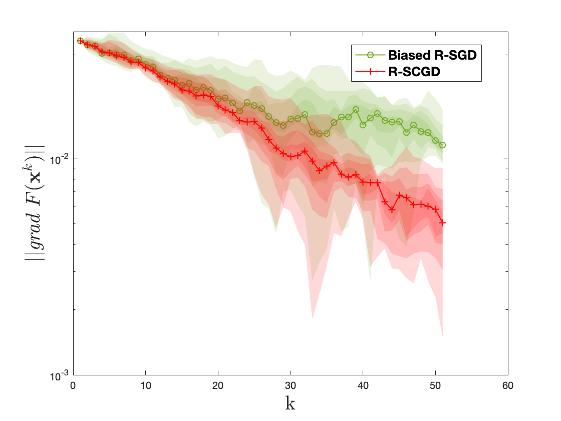
Figure 1: Comparison between the biased R-SGD and R-SCGD

5 Conclusion

We present the Riemannian stochastic compositional gradient method (R-SCGD) to solve composition of two or multiple functions involving expectations over Riemannian manifolds. The proposed algorithm which is motivated by the Riemannian gradient flow approximates the inner function(s) value(s) using a moving average corrected by first-order information and its parameter(s) is in the same timescale as the stepsize of the variable update. We established the sample complexity of $\mathcal{O}(1/\epsilon^{2})$ for the proposed algorithms to obtain $\epsilon$-approximate stationary solution, i.e., $\|\text{grad}f(x)\|^{2}\leq\epsilon$. We empirically studied the performance of the proposed algorithm over a policy approximation example in reinforcement learning.

Appendices

We provide the proofs related to the complexity analysis of the two-level and multi-level R-SCGD algorithms. The assumptions for the analysis of the multi-level R-SCGD algorithm, which are omitted from the body of the paper, are stated in Section B.

A Complexity analysis of the two-level R-SCGD

A.1 Proof of Lemma 2.1

Proof.

It suffices to show that

$$\left\langle\mathbb{E}[(Dg_{\phi}(\mathbf{x}))^{*}\text{Proj}_{g_{\phi}(\mathbf{x})}\nabla f_{\xi}(g(\mathbf{x}))],b_{i}\right\rangle_{\mathbf{x}}=\left\langle(Dg(\mathbf{x}))^{*}\text{Proj}_{g(\mathbf{x})}\nabla f(g(\mathbf{x})),b_{i}\right\rangle_{\mathbf{x}},$$ (36)

where $\left\langle\cdot,\cdot\right\rangle_{\mathbf{x}}$ is the inner product defined on the tangent plane of the manifold $\mathcal{M}$ at $\mathbf{x}$, i.e. $T_{\mathbf{x}}\mathcal{M}$, and $\{b_{i}\}$ is the basis of $T_{\mathbf{x}}\mathcal{M}$. We have

$$\left\langle\mathbb{E}[(Dg_{\phi}(\mathbf{x}))^{*}\text{Proj}_{g_{\phi}(\mathbf{x})}\nabla f_{\xi}(g(\mathbf{x}))],b_{i}\right\rangle_{\mathbf{x}}$$ (37)

$$\stackrel{{\scriptstyle\textnormal{(a)}}}{{\mathstrut{=}}}\mathbb{E}\left\langle\text{Proj}_{g_{\phi}(\mathbf{x})}\nabla f_{\xi}(g(\mathbf{x})),Dg_{\phi}(\mathbf{x})[b_{i}]\right\rangle_{g_{\phi}(\mathbf{x})}$$ (38)

$$\stackrel{{\scriptstyle\textnormal{(b)}}}{{\mathstrut{=}}}\mathbb{E}\left\langle\nabla f_{\xi}(g(\mathbf{x})),Dg_{\phi}(\mathbf{x})[b_{i}]\right\rangle$$ (39)

$$\stackrel{{\scriptstyle\textnormal{(c)}}}{{\mathstrut{=}}}\left\langle\nabla f(g(\mathbf{x})),Dg(\mathbf{x})[b_{i}]\right\rangle$$ (40)

$$\stackrel{{\scriptstyle\textnormal{(d)}}}{{\mathstrut{=}}}\left\langle(Dg(\mathbf{x}))^{*}\text{Proj}_{g(\mathbf{x})}\nabla f(g(\mathbf{x})),b_{i}\right\rangle_{\mathbf{x}}.$$ (41)

The equality (38) comes from the linearity of the inner product and the definition of adjoint operator (see Definition 3). For the equality (39), since we assume the manifold $\mathcal{N}$ is embedded in the Euclidean space $\mathcal{E}$, the inner product is the induced metric inherited from the Euclidean metric (Boumal 2020) and the orthogonal projection operator can be erased. The equality (40) follows from the independence between random variables $\xi$ and $\phi$. Finally, the last equality (41) follows from the definition of adjoint operator. ∎

A.2 Proof of Lemma 2.2

Proof.

Under the update rule

$$\mathbf{y}^{k+1}=\mathbf{y}^{k}-\beta_{k}(\mathbf{y}^{k}-g_{\phi^{k}}(\mathbf{x}^{k}))+\gamma_{k}(g_{\phi^{k}}(\mathbf{x}^{k})-g_{\phi^{k}}(\mathbf{x}^{k-1})),$$

we have

$$\mathbf{y}^{k+1}-g(\mathbf{x}^{k})=(1-\beta_{k})(\mathbf{y}^{k}-g(\mathbf{x}^{k-1}))+(1-\beta_{k})T_{1,k}+\beta_{k}T_{2,k}+\gamma_{k}T_{3,k},$$ (42)

where $T_{1,k}:=g(\mathbf{x}^{k-1})-g(\mathbf{x}^{k})$, $T_{2,k}:=g_{\phi^{k}}(\mathbf{x}^{k})-g(\mathbf{x}^{k})$, $T_{3,k}:=g_{\phi^{k}}(\mathbf{x}^{k})-g_{\phi^{k}}(\mathbf{x}^{k-1})$. Conditioned on $\mathcal{F}^{k}$, taking expectation over $\phi^{k}$, we have

$$\mathbb{E}[(1-\beta_{k})T_{1,k}+\beta_{k}T_{2,k}+\gamma_{k}T_{3,k}|\mathcal{F}^{k}]=(1-\beta_{k}-\gamma_{k})T_{1,k},$$ (43)

where we have used the condition $\mathbb{E}[g_{\phi}(\mathbf{x})]=g(\mathbf{x})$ in the Assumption 2.3.

Therefore, conditioned on $\mathcal{F}^{k}$, taking expectation on the both sides of (42), we have

$$\mathbb{E}[\|\mathbf{y}^{k+1}-g(\mathbf{x}^{k})\|^{2}|\mathcal{F}^{k}]$$

$$= \mathbb{E}[\|(1-\beta_{k})(\mathbf{y}^{k}-g(\mathbf{x}^{k-1}))\|^{2}|\mathcal{F}^{k}]+\mathbb{E}[\|(1-\beta_{k})T_{1,k}+\beta_{k}T_{2,k}+\gamma_{k}T_{3,k}\|^{2}|\mathcal{F}^{k}]$$

$$+2\mathbb{E}[\left\langle(1-\beta_{k})(\mathbf{y}^{k}-g(\mathbf{x}^{k-1})),(1-\beta_{k})T_{1,k}+\beta_{k}T_{2,k}+\gamma_{k}T_{3,k}\right\rangle|\mathcal{F}^{k}]$$

$$\leq (1-\beta_{k})^{2}\|\mathbf{y}^{k}-g(\mathbf{x}^{k-1})\|^{2}+2\mathbb{E}[\|(1-\beta_{k})T_{1,k}+\beta_{k}T_{2,k}\|^{2}|\mathcal{F}^{k}]+2\gamma_{k}^{2}\mathbb{E}[\|T_{3,k}\|^{2}|\mathcal{F}^{k}]$$

$$+2(1-\beta_{k})(1-\beta_{k}-\gamma_{k})\|\mathbf{y}^{k}-g(\mathbf{x}^{k-1})\|\cdot\|T_{1,k}\|$$

$$\stackrel{{\scriptstyle\textnormal{(e)}}}{{\mathstrut{\leq}}} (1-\beta_{k})^{2}\|\mathbf{y}^{k}-g(\mathbf{x}^{k-1})\|^{2}+2(1-\beta_{k})^{2}\|T_{1,k}\|^{2}+2\beta_{k}^{2}\mathbb{E}[\|T_{2,k}\|^{2}|\mathcal{F}^{k}]+2\gamma_{k}^{2}\mathbb{E}[|\|T_{3,k}\|^{2}|\mathcal{F}^{K}]$$

$$+(1-\beta_{k})^{2}\beta_{k}\|\mathbf{y}^{k}-g(\mathbf{x}^{k-1})\|^{2}+\frac{(1-\beta_{k}-\gamma_{k})^{2}}{\beta_{k}}\|T_{1,k}\|^{2}$$

$$\stackrel{{\scriptstyle\textnormal{(f)}}}{{\mathstrut{\leq}}} (1-\beta_{k})\|\mathbf{y}^{k}-g(\mathbf{x}^{k-1})\|^{2}+2\beta_{k}^{2}V_{g}^{2}+(2(1-\beta_{k})^{2}+2\gamma_{k}^{2}+\frac{(1-\beta_{k}-\gamma_{k})^{2}}{\beta_{k}})\alpha_{k}^{2}C_{g}^{4}C_{f}^{2}$$

where (A.2) is based on the Young’s inequality; (A.2) uses the updating rule of $\mathbf{y}^{k+1}$ (see the Algorithm 1) and Assumptions 2.3 and 2.5. ∎

A.3 Proof of Theorem 2.1

Proof.

Using the smoothness of $F(\mathbf{x}^{k})$ (see Assumption 2.1), we have

$$F(\mathbf{x}^{k+1})\leq F(\mathbf{x}^{k})-\alpha_{k}\left\langle\eta^{k+1},\text{grad }F(\mathbf{x}^{k})\right\rangle+\frac{\alpha_{k}^{2}L_{F}}{2}\|\eta^{k+1}\|^{2}$$ (44)

$$= F(\mathbf{x}^{k})-\alpha_{k}\|\text{grad }F(\mathbf{x}^{k})\|^{2}+\frac{\alpha_{k}^{2}L_{F}}{2}\|\eta^{k+1}\|^{2}$$ (45)

$$+ \alpha_{k}\left\langle\text{grad}F(\mathbf{x}^{k}),(Dg(\mathbf{x}^{k}))^{*}\text{Proj}_{g(\mathbf{x}^{k})}\nabla f(g(\mathbf{x}^{k}))-(Dg_{\phi^{k}}(\mathbf{x}^{k}))^{*}\text{Proj}_{g_{\phi^{k}}(\mathbf{x}^{k})}\nabla f_{\xi^{k}}(\mathbf{y}^{k+1})\right\rangle,$$ (46)

where the first inequality comes from the Proposition 10.47 in Boumal (2020).

Conditioned on $\mathcal{F}^{k}$, taking expectation over $\phi^{k}$ and $\xi^{k}$ on both sides, we have

$$\mathbb{E}[F(\mathbf{x}^{k+1})|\mathcal{F}^{k}]$$ (47)

$$\stackrel{{\scriptstyle\textnormal{(g)}}}{{\mathstrut{\leq}}} F(\mathbf{x}^{k})-\alpha_{k}\|\text{grad }F(\mathbf{x}^{k})\|^{2}+\frac{\alpha_{k}^{2}L_{F}}{2}\mathbb{E}[\|\eta^{k+1}\|^{2}|\mathcal{F}^{k}]$$ (48)

$$+ \alpha_{k}\mathbb{E}[\left\langle\text{grad}F(\mathbf{x}^{k}),(Dg_{\phi^{k}}(\mathbf{x}^{k}))^{*}\text{Proj}_{g_{\phi^{k}}(\mathbf{x}^{k})}(\nabla f_{\xi^{k}}(g(\mathbf{x}^{k}))-\nabla f_{\xi^{k}}(\mathbf{y}^{k+1}))\right\rangle|\mathcal{F}^{k}]$$ (49)

$$\stackrel{{\scriptstyle\textnormal{(h)}}}{{\mathstrut{\leq}}} F(\mathbf{x}^{k})-\alpha_{k}\|\text{grad }F(\mathbf{x}^{k})\|^{2}+\frac{\alpha_{k}^{2}L_{F}}{2}\mathbb{E}[\|\eta^{k+1}\|^{2}|\mathcal{F}^{k}]$$ (50)

$$+ \alpha_{k}\|\text{grad}F(\mathbf{x}^{k})\|\cdot\mathbb{E}[\|Dg(\mathbf{x}^{k})[\cdot]\|_{op}^{2}|\mathcal{F}^{k}]^{1/2}\cdot\mathbb{E}[\|\nabla f(g(\mathbf{x}^{k}))-\nabla f(\mathbf{y}^{k+1})\|^{2}|\mathcal{F}^{k}]^{1/2}$$ (51)

$$\stackrel{{\scriptstyle\textnormal{(i)}}}{{\mathstrut{\leq}}} F(\mathbf{x}^{k})-\alpha_{k}\|\text{grad }F(\mathbf{x}^{k})\|^{2}+\frac{L_{F}}{2}\alpha_{k}^{2}C_{g}^{2}C_{f}^{2}$$ (52)

$$+ \alpha_{k}C_{g}L_{f}\cdot\|\text{grad}F(\mathbf{x}^{k})\|\cdot\mathbb{E}[\|g(\mathbf{x}^{k})-\mathbf{y}^{k+1}\|^{2}|\mathcal{F}^{k}]^{1/2}$$ (53)

$$\stackrel{{\scriptstyle\textnormal{(j)}}}{{\mathstrut{\leq}}} F(\mathbf{x}^{k})-\alpha_{k}(1-\frac{\alpha_{k}}{4\beta_{k}}C_{g}^{2}L_{f}^{2})\|\text{grad }F(\mathbf{x}^{k})\|^{2}+\frac{L_{F}}{2}\alpha_{k}^{2}C_{g}^{2}C_{f}^{2}+\beta_{k}\mathbb{E}[\|g(\mathbf{x}^{k})-\mathbf{y}^{k+1}\|^{2}|\mathcal{F}^{k}].$$ (54)

The inequality (48) follows from Assumption 2.4; The inequality (50) uses the Cauchy-Schwartz inequality and nonexpansiveness property of the projection operator; The inequality (52) is based on Assumptions 2.2, 2.5 and the Jensen inequality; Finally, the inequality (54) uses the Young’s inequality. Based on the definition of the Lyapunov function in (16), it follows that

$$\mathbb{E}[\mathcal{V}^{k+1}|\mathcal{F}^{k}]-\mathcal{V}^{k} \leq-\alpha_{k}(1-\frac{\alpha_{k}}{4\beta_{k}}C_{g}^{2}L_{f}^{2})\|\text{grad }F(\mathbf{x}^{k})\|^{2}+\frac{L_{F}}{2}\alpha_{k}^{2}C_{g}^{2}C_{f}^{2}$$ (55)

$$+(1+\beta_{k})\mathbb{E}[\|g(\mathbf{x}^{k})-\mathbf{y}^{k+1}\|^{2}|\mathcal{F}^{k}]-\|g(\mathbf{x}^{k-1})-\mathbf{y}^{k}\|^{2}.$$ (56)

In the following, we enforce $\beta_{k}=\frac{\alpha_{k}C_{g}^{2}L^{2}_{f}}{2}$, and $\alpha_{k}$ sufficiently small such that $\beta_{k}\in(0,1)$. Combining the result in the Lemma 2.2, we have

$$\mathbb{E}[\mathcal{V}^{k+1}|\mathcal{F}^{k}]-\mathcal{V}^{k} \leq-\frac{\alpha_{k}}{2}\|\text{grad }F(\mathbf{x}^{k})\|^{2}+\frac{L_{F}}{2}\alpha_{k}^{2}C_{g}^{2}C_{f}^{2}-\beta_{k}^{2}\|g(\mathbf{x}^{k-1})-\mathbf{y}^{k}\|^{2}$$ (57)

$$+\frac{1+\beta_{k}}{2}\alpha_{k}^{2}C_{g}^{4}L_{f}^{4}V_{g}^{2}+[2+6(t+1)^{2}]\alpha_{k}^{2}C_{g}^{4}C_{f}^{2}$$ (58)

$$\leq-\frac{\alpha_{k}}{2}\|\text{grad }F(\mathbf{x}^{k})\|^{2}+\frac{L_{F}}{2}\alpha_{k}^{2}C_{g}^{2}C_{f}^{2}$$ (59)

$$\alpha_{k}^{2}C_{g}^{4}L_{f}^{4}V_{g}^{2}+[2+6(t+1)^{2}]\alpha_{k}^{2}C_{g}^{4}C_{f}^{2}$$ (60)

Defining $B:=\frac{L_{F}}{2}C_{g}^{2}C_{f}^{2}+C_{g}^{4}L_{f}^{4}V_{g}^{2}+[2+6(t+1)^{2}]C_{g}^{4}C_{f}^{2}$, and taking expectation over $\mathcal{F}^{k}$ on both sides of the above inequality, it follows that

$$\mathbb{E}[\mathcal{V}^{k+1}]\leq\mathbb{E}[\mathcal{V}^{k}]-\frac{\alpha_{k}}{2}\mathbb{E}[\|\text{grad }F(\mathbf{x}^{k})\|^{2}]+B\alpha_{k}^{2}.$$ (61)

By telescoping, we have

$$\mathbb{E}[\mathcal{V}^{K}]\leq\mathcal{V}^{0}-\frac{1}{2}\sum_{k=0}^{K-1}\alpha_{k}\mathbb{E}[\|\text{grad }F(\mathbf{x}^{k})\|^{2}]+B\sum_{k=0}^{K-1}\alpha_{k}^{2}.$$ (62)

. Using the fact that $\mathbb{E}[\mathcal{V}^{K}]\geq 0$ and rearranging the terms, we have

$$\frac{\sum_{k=0}^{K-1}\alpha_{k}\mathbb{E}[\|\text{grad }F(\mathbf{x}^{k})\|^{2}]}{\sum_{k=0}^{K-1}\alpha_{k}}\leq\frac{2\mathcal{V}^{0}+2B\sum_{k=0}^{K-1}\alpha_{k}^{2}}{\sum_{k=0}^{K-1}\alpha_{k}}.$$ (63)

Choosing the stepsize as $\alpha_{k}=\frac{1}{\sqrt{{K}}}$ leads

$$\frac{\sum_{k=0}^{K-1}\mathbb{E}[\|\text{grad }F(\mathbf{x}^{k})\|^{2}]}{K}\leq\frac{2\mathcal{V}^{0}+2B}{\sqrt{K}},$$ (64)

from which the proof is complete. ∎

B Complexity analysis of the multi-level R-SCGD

B.1 Proof of Lemma 3.1

Proof.

Let $\mathcal{F}^{k,n}$ denotes the $\sigma$-algebra generated by $\mathcal{F}^{k}\cup\{\theta^{k}_{i},1\leq i\leq n-1\}$. From the update scheme for $\mathbf{y}_{n}^{k+1}$ (similarly when $n=1$), we have

$$\mathbf{y}_{n}^{k+1}-f_{n}(\mathbf{y}^{k+1}_{n-1}) =(1-\beta_{k})(\mathbf{y}_{n}^{k}-f_{n}(\mathbf{y}^{k}_{n-1}))+(1-\beta_{k})(f_{n}(\mathbf{y}^{k}_{n-1})-f_{n}(\mathbf{y}^{k+1}_{n-1}))$$ (65)

$$+\beta_{k}(f_{n}(\mathbf{y}^{k+1}_{n-1};\theta^{k}_{n})-f_{n}(\mathbf{y}_{n-1}^{k+1}))+\gamma_{k}(f_{n}(\mathbf{y}^{k+1}_{n-1};\theta^{k}_{n})-f_{n}(\mathbf{y}_{n-1}^{k};\theta^{k}_{n}))$$ (66)

$$=(1-\beta_{k})(\mathbf{y}_{n}^{k}-f_{n}(\mathbf{y}_{n-1}^{k}))+(1-\beta_{k})T_{1}+\beta_{k}T_{2}+\gamma_{k}T_{3}$$ (67)

where $T_{1}:=f_{n}(\mathbf{y}^{k}_{n-1})-f_{n}(\mathbf{y}^{k+1}_{n-1})$, $T_{2}:=f_{n}(\mathbf{y}^{k+1}_{n-1};\theta^{k}_{n})-f_{n}(\mathbf{y}_{n-1}^{k+1})$ and $T_{3}:=f_{n}(\mathbf{y}^{k+1}_{n-1};\theta^{k}_{n})-f_{n}(\mathbf{y}_{n-1}^{k};\theta^{k}_{n})$.

Conditioned on $\mathcal{F}^{k,n}$, taking expectation over $\theta^{k}_{n}$, we have

$$\mathbb{E}[(1-\beta_{k})T_{1}+\beta_{2}T_{2}+\gamma_{k}T_{3}|\mathcal{F}^{k,n}]=(1-\beta_{k}-\gamma_{k})T_{1}.$$ (68)

where we have used Assumption 3.2.

Based on the (67), we have

$$\mathbb{E}[\|\mathbf{y}_{n}^{k+1}-f_{n}(\mathbf{y}_{n-1}^{k+1})\|^{2}|\mathcal{F}^{k,n}]$$

$$\stackrel{{\scriptstyle\textnormal{(k)}}}{{\mathstrut{=}}} (1-\beta_{k})^{2}\|\mathbf{y}^{k}_{n}-f_{n}(\mathbf{y}^{k}_{n-1})\|^{2}+\mathbb{E}[\|(1-\beta_{k})T_{1}+\beta_{k}T_{2}+\gamma_{k}T_{3}\|^{2}|\mathcal{F}^{k,n}]$$

$$+2(1-\beta_{k})(1-\beta_{k}-\gamma_{k})\|\mathbf{y}^{k}_{n}-f_{n}(\mathbf{y}^{k}_{n-1})\|\cdot\|T_{1}\|$$

$$\leq (1-\beta_{k})^{2}\|\mathbf{y}^{k}_{n}-f_{n}(\mathbf{y}^{k}_{n-1})\|^{2}+2\mathbb{E}[\|(1-\beta_{k})T_{1}+\beta_{k}T_{2}\|^{2}|\mathcal{F}^{k,n}]+2\gamma_{k}^{2}\mathbb{E}[\|T_{3}\|^{2}|\mathcal{F}^{k,n}]$$

$$+(1-\beta_{k})^{2}\beta_{k}\|\mathbf{y}^{k}_{n}-f_{n}(\mathbf{y}^{k}_{n-1})\|^{2}+\frac{(1-\beta_{k}-\gamma_{k})^{2}}{\beta_{k}}\|T_{1}\|^{2}$$

$$\stackrel{{\scriptstyle\textnormal{(l)}}}{{\mathstrut{\leq}}} (1-\beta_{k})\|\mathbf{y}^{k}_{n}-f_{n}(\mathbf{y}^{k}_{n-1})\|^{2}+[2(1-\beta_{k})^{2}+\frac{(1-\beta_{k}-\gamma_{k})^{2}}{\beta_{k}}]\|T_{1}\|^{2}++2\gamma_{k}^{2}\mathbb{E}[\|T_{3}\|^{2}|\mathcal{F}^{k,n}]$$

$$+ 2\beta_{k}^{2}\mathbb{E}[\|T_{2}\||\mathcal{F}^{k,n}]$$

$$\stackrel{{\scriptstyle\textnormal{(m)}}}{{\mathstrut{\leq}}} (1-\beta_{k})\|\mathbf{y}^{k}_{n}-f_{n}(\mathbf{y}^{k}_{n-1})\|^{2}+[2(1-\beta_{k})^{2}+\frac{(1-\beta_{k}-\gamma_{k})^{2}}{\beta_{k}}+2\gamma_{k}^{2}]C_{n}^{2}\|\mathbf{y}^{k}_{n-1}-\mathbf{y}^{k+1}_{n-1}\|^{2}+2\beta_{k}^{2}V_{n}^{2},$$

where (B.1) follows from the equality (68); (B.1) is based on the fact that

$$\mathbb{E}[\left\langle T_{1},T_{2}\right\rangle|\mathcal{F}^{k,n}]=\left\langle T_{1},\mathbb{E}[T_{2}|\mathcal{F}^{k,n}]\right\rangle=0\text{ and }(1-\beta_{k})^{2}(1+\beta_{k})\leq 1-\beta_{k};$$

and the last inequality (B.1) follows from Assumptions 3.2 and 3.4.

Due to the law of total expectation (see e.g. Billingsley (2008)),

$$\mathbb{E}[\|\mathbf{y}_{n}^{k+1}-f_{n}(\mathbf{y}_{n-1}^{k+1})\|^{2}|\mathcal{F}^{k}]$$

$$= \mathbb{E}[\mathbb{E}[\|\mathbf{y}_{n}^{k+1}-f_{n}(\mathbf{y}_{n-1}^{k+1})\|^{2}|\mathcal{F}^{k,n}]|\mathcal{F}^{k}]$$

$$\leq (1-\beta_{k})\|\mathbf{y}^{k}_{n}-f_{n}(\mathbf{y}^{k}_{n-1})\|^{2}+[2(1-\beta_{k})^{2}+\frac{(1-\beta_{k}-\gamma_{k})^{2}}{\beta_{k}}+2\gamma_{k}^{2}]C_{n}^{2}\|\mathbf{y}^{k}_{n-1}-\mathbf{y}^{k+1}_{n-1}\|^{2}+2\beta_{k}^{2}V_{n}^{2}.$$

∎

B.2 Proof of Theorem 3.1

Proof.

Using the smoothness of $F(\mathbf{x}^{k})$ (see Assumption 2.1), we have

$$F(\mathbf{x}^{k+1}) \leq F(\mathbf{x}^{k})-\alpha_{k}\left\langle\eta^{k+1},\text{grad }F(\mathbf{x}^{k})\right\rangle+\frac{\alpha_{k}^{2}L_{F}}{2}\|\eta^{k+1}\|^{2}$$

$$=F(\mathbf{x}^{k})-\alpha_{k}\|\text{grad }F(\mathbf{x}^{k})\|^{2}+\frac{\alpha_{k}^{2}L_{F}}{2}\|\eta^{k+1}\|^{2}+\alpha_{k}\left\langle\text{grad}F(\mathbf{x}^{k}),\text{grad}F(\mathbf{x}^{k})-\eta^{k+1}\right\rangle,$$

where the first inequality comes from the Proposition 10.47 in Boumal (2020). Conditioned on $\mathcal{F}^{k}$, taking expectation over $\theta_{1}^{k}$,…,$\theta_{N}^{k}$, we have

$$\mathbb{E}[F(\mathbf{x}^{k+1})|\mathcal{F}^{k}]$$

$$\leq F(\mathbf{x}^{k})-\alpha_{k}\|\text{grad}F(\mathbf{x}^{k})\|^{2}+\frac{\alpha_{k}^{2}L_{F}}{2}\mathbb{E}[\|\eta^{k+1}\|^{2}|\mathcal{F}^{k}]+\alpha_{k}\left\langle\text{grad}F(\mathbf{x}^{k}),\text{grad}F(\mathbf{x}^{k})-\mathbb{E}[\eta^{k+1}|\mathcal{F}^{k}]\right\rangle$$

$$\leq F(\mathbf{x}^{k})-\alpha_{k}\|\text{grad}F(\mathbf{x}^{k})\|^{2}+\frac{\alpha_{k}^{2}L_{F}}{2}\prod_{i=n}^{N}C_{n}^{2}+\alpha_{k}\|\text{grad}F(\mathbf{x}^{k})\|\cdot\|\text{grad}F(\mathbf{x}^{k})-\mathbb{E}[\eta^{k+1}|\mathcal{F}^{k}]\|$$

$$\stackrel{{\scriptstyle\textnormal{(a)}}}{{\mathstrut{\leq}}} F(\mathbf{x}^{k})-\alpha_{k}\|\text{grad}F(\mathbf{x}^{k})\|^{2}+\frac{\alpha_{k}^{2}L_{F}}{2}\prod_{n=1}^{N}C_{n}^{2}+\alpha_{k}\sum_{n=1}^{N-1}A_{n}\|\text{grad}F(\mathbf{x}^{k})\|\cdot\mathbb{E}[\|\mathbf{y}_{n}^{k+1}-f_{n}(\mathbf{y}^{k+1}_{n-1})\||\mathcal{F}^{k}]$$

$$\stackrel{{\scriptstyle\textnormal{(b)}}}{{\mathstrut{\leq}}} F(\mathbf{x}^{k})-\alpha_{k}(1-\frac{\alpha_{k}}{4\beta_{k}}\sum_{n=1}^{N-1}A_{n}^{2})\|\text{grad}F(\mathbf{x}^{k})\|^{2}+\beta_{k}\sum_{n=1}^{N-1}\mathbb{E}[\|\mathbf{y}_{n}^{k+1}-f_{n}(\mathbf{y}_{n-1}^{k+1})\|^{2}|\mathcal{F}^{k}]+\frac{\alpha_{k}^{2}L_{F}}{2}\prod_{n=1}^{N}C_{n}^{2},$$

where $A_{n}:=\sum_{m=n+1}^{N-1}C_{N}\cdots C_{m+1}C_{m-1}\cdots C_{1}L_{m}\cdots L_{n+1}$. Inequality (B.2) is based on Assumption 3.3 and follows exactly the proof in Chen et al. (2021); the inequality (B.2) follows from the Young’s inequality. Based on the definition of generalized Lyapunov function (27), we have

$$\mathbb{E}[\mathcal{V}^{k+1}|\mathcal{F}^{k}] -\mathcal{V}^{k}\leq\mathbb{E}[F(\mathbf{x}^{k+1})|\mathcal{F}^{k}]+\mathbb{E}[\sum_{n=1}^{N-1}\|\mathbf{y}_{n}^{k+1}-f_{n}(\mathbf{y}_{n-1}^{k+1})\|^{2}|\mathcal{F}^{k}]-F(\mathbf{x}^{k})-\sum_{n=1}^{N-1}\|\mathbf{y}_{n}^{k}-f_{n}(\mathbf{y}_{n-1}^{k})\|^{2}$$

$$\leq -\alpha_{k}(1-\frac{\alpha_{k}}{4\beta_{k}}\sum_{n=1}^{N-1}A_{n}^{2})\|\text{grad}F(\mathbf{x}^{k})\|^{2}+(\beta_{k}+1)\sum_{n=1}^{N-1}\mathbb{E}[\|\mathbf{y}_{n}^{k+1}-f_{n}(\mathbf{y}_{n-1}^{k+1})\|^{2}|\mathcal{F}^{k}]$$

$$+\frac{\alpha_{k}^{2}L_{F}}{2}\prod_{n=1}^{N}C_{n}^{2}-\sum_{n=1}^{N-1}\|\mathbf{y}_{n}^{k}-f_{n}(\mathbf{y}_{n-1}^{k})\|^{2}$$

$$=-\frac{\alpha_{k}}{2}\|\text{grad}F(\mathbf{x}^{k})\|^{2}+(2\beta_{k}+1)\sum_{n=1}^{N-1}\mathbb{E}[\|\mathbf{y}_{n}^{k+1}-f_{n}(\mathbf{y}_{n-1}^{k+1})\|^{2}|\mathcal{F}^{k}]+\frac{\alpha_{k}^{2}L_{F}}{2}\prod_{n=1}^{N}C_{n}^{2}$$

$$-\beta_{k}\sum_{n=1}^{N-1}\mathbb{E}[\|\mathbf{y}_{n}^{k+1}-f_{n}(\mathbf{y}_{n-1}^{k+1})\|^{2}|\mathcal{F}^{k}]-\sum_{n=1}^{N-1}\|\mathbf{y}_{n}^{k}-f_{n}(\mathbf{y}_{n-1}^{k})\|^{2},$$

where in the last equality we set

$$\beta_{k}:=\frac{\alpha_{k}}{2}\sum_{n=1}^{N-1}A_{n}^{2}.$$ (69)

Before we combine the above inequality with the result in Lemma 3.1, we consider the following quantities,

$$\begin{split}&(2\beta_{k}+1)(1-\beta_{k})\leq 1\text{ when }0\leq\beta_{k}\leq 1,\\ &[2(1-\beta_{k})^{2}+\frac{(1-\beta_{k}-\gamma_{k})^{2}}{\beta_{k}}+2\gamma_{k}^{2}](2\beta_{k}+1)\leq M_{1}:=2+3(t+1)(t+2),\end{split}$$ (70)

where we choose

$$\gamma_{k}=1-t_{k}\beta_{k}\text{ such that }t:=\sup\{|t_{k}|\}\text{ is finite}.$$ (71)

Using the quantities (70) and Lemma 3.1, we have

$$\begin{split}&\mathbb{E}[\mathcal{V}^{k+1}|\mathcal{F}^{k}]-\mathcal{V}^{k}\\ &\leq-\frac{\alpha_{k}}{2}\|\text{grad}F(\mathbf{x}^{k})\|^{2}+M_{1}\sum_{n=1}^{N-1}C_{n}^{2}\mathbb{E}[\|\mathbf{y}^{k}_{n-1}-\mathbf{y}^{k+1}_{n-1}\|^{2}|\mathcal{F}^{k}]+2\beta_{k}^{2}(2\beta_{k}+1)\sum_{n=1}^{N-1}V_{n}^{2}\\ &+\frac{\alpha_{k}^{2}L_{F}}{2}\prod_{n=1}^{N}C_{n}^{2}-\beta_{k}\sum_{n=1}^{N-1}\mathbb{E}[\|\mathbf{y}_{n}^{k+1}-f_{n}(\mathbf{y}_{n-1}^{k+1})\|^{2}|\mathcal{F}^{k}]\\ &=-\frac{\alpha_{k}}{2}\|\text{grad}F(\mathbf{x}^{k})\|^{2}+M_{1}C_{1}^{2}\alpha_{k}^{2}\mathbb{E}[\|\eta^{k}\|^{2}|\mathcal{F}^{k}]+2\beta_{k}^{2}(2\beta_{k}+1)\sum_{n=1}^{N-1}V_{n}^{2}+\frac{\alpha_{k}^{2}L_{F}}{2}\prod_{n=1}^{N}C_{n}^{2}\\ &+\sum_{n=2}^{N-1}(M_{1}C_{n}^{2}+\psi_{n})\mathbb{E}[\|\mathbf{y}_{n-1}^{k}-\mathbf{y}_{n-1}^{k+1}\|^{2}|\mathcal{F}^{k}]-\sum_{n=2}^{N-1}\psi_{n}\mathbb{E}[\|\mathbf{y}_{n-1}^{k}-\mathbf{y}_{n-1}^{k+1}\|^{2}|\mathcal{F}^{k}]\\ &-\beta_{k}\sum_{n=1}^{N-1}\mathbb{E}[\|\mathbf{y}_{n}^{k+1}-f_{n}(\mathbf{y}_{n-1}^{k+1})\|^{2}|\mathcal{F}^{k}].\end{split}$$ (72)

The parameters $\psi_{n}$ will be carefully chosen such that the last three terms are upper bounded by certain constants. Due to the updating rule for $\mathbf{y}_{n}^{k+1}$ in Algorithm 2, we have

$$(1-\beta_{k})(\mathbf{y}_{n-1}^{k+1}-\mathbf{y}_{n-1}^{k})=\beta_{k}(f_{n-1}(\mathbf{y}_{n-2}^{k+1};\theta_{n-1}^{k})-\mathbf{y}_{n-1}^{k+1})+\gamma_{k}(f_{n-1}(\mathbf{y}_{n-2}^{k+1};\theta_{n-1}^{k})-f_{n-1}(\mathbf{y}_{n-2}^{k};\theta_{n-1}^{k}))$$ (73)

Conditioned on $\mathcal{F}^{k}$, we have

$$\begin{split}&\mathbb{E}[\|\mathbf{y}_{n-1}^{k+1}-\mathbf{y}_{n-1}^{k}\|^{2}|\mathcal{F}^{k}]\\ &\leq 2(\frac{\beta_{k}}{1-\beta_{k}})^{2}\mathbb{E}[\|f_{n-1}(\mathbf{y}_{n-2}^{k+1};\theta_{n-1}^{k})-f_{n-1}(\mathbf{y}_{n-2}^{k+1})+f_{n-1}(\mathbf{y}_{n-2}^{k+1})-\mathbf{y}_{n-1}^{k+1}\|^{2}|\mathcal{F}^{k}]\\ &+2(\frac{\gamma_{k}}{1-\beta_{k}})^{2}\mathbb{E}[\|f_{n-1}(\mathbf{y}_{n-2}^{k+1};\theta_{n-1}^{k})-f_{n-1}(\mathbf{y}_{n-2}^{k};\theta_{n-1}^{k})\|^{2}|\mathcal{F}^{k}]\\ &\leq 2(\frac{\beta_{k}}{1-\beta_{k}})^{2}V_{n-1}^{2}+2(\frac{\beta_{k}}{1-\beta_{k}})^{2}\mathbb{E}[\|f_{n-1}(\mathbf{y}_{n-2}^{k+1})-\mathbf{y}_{n-1}^{k+1}\|^{2}|\mathcal{F}^{k}]\\ &+2(\frac{\gamma_{k}}{1-\beta_{k}})^{2}C_{n-1}^{2}\mathbb{E}[\|\mathbf{y}_{n-2}^{k+1}-\mathbf{y}_{n-2}^{k}\|^{2}|\mathcal{F}^{k}]\\ &\leq 2(\frac{\beta_{k}}{1-\beta_{k}})^{2}V_{n-1}^{2}+2(\frac{\beta_{k}}{1-\beta_{k}})^{2}\mathbb{E}[\|f_{n-1}(\mathbf{y}_{n-2}^{k+1})-\mathbf{y}_{n-1}^{k+1}\|^{2}|\mathcal{F}^{k}]\\ &+2t^{2}C_{n-1}^{2}\mathbb{E}[\|\mathbf{y}_{n-2}^{k+1}-\mathbf{y}_{n-2}^{k}\|^{2}|\mathcal{F}^{k}].\end{split}$$ (74)

Plugging (74) into (72), we have

$$\begin{split}\mathbb{E}[\mathcal{V}^{k+1}|\mathcal{F}^{k}]&-\mathcal{V}^{k}\leq-\frac{\alpha_{k}}{2}\|\text{grad}F(\mathbf{x}^{k})\|^{2}+M_{1}C_{1}^{2}\alpha_{k}^{2}\mathbb{E}[\|\eta^{k}\|^{2}|\mathcal{F}^{k}]+2\beta_{k}^{2}(2\beta_{k}+1)\sum_{n=1}^{N-1}V_{n}^{2}\\ &+\frac{\alpha_{k}^{2}L_{F}}{2}\prod_{n=1}^{N}C_{n}^{2}-\sum_{n=2}^{N-1}\psi_{n}\mathbb{E}[\|\mathbf{y}_{n-1}^{k}-\mathbf{y}_{n-1}^{k+1}\|^{2}|\mathcal{F}^{k}]-\beta_{k}\sum_{n=1}^{N-1}\mathbb{E}[\|\mathbf{y}_{n}^{k+1}-f_{n}(\mathbf{y}_{n-1}^{k+1})\|^{2}|\mathcal{F}^{k}]\\ &+2(\frac{\beta_{k}}{1-\beta_{k}})^{2}\sum_{n=2}^{N-1}(M_{1}C_{n}^{2}+\psi_{n})V_{n-1}^{2}\\ &+2(\frac{\beta_{k}}{1-\beta_{k}})^{2}\sum_{n=2}^{N-1}(M_{1}C_{n}^{2}+\psi_{n})\mathbb{E}[\|f_{n-1}(\mathbf{y}_{n-2}^{k+1})-\mathbf{y}_{n-1}^{k+1}\|^{2}|\mathcal{F}^{k}]\\ &+2t^{2}\sum_{n=2}^{N-1}(M_{1}C_{n}^{2}+\psi_{n})C_{n-1}^{2}\mathbb{E}[\|\mathbf{y}_{n-2}^{k+1}-\mathbf{y}_{n-2}^{k}\|^{2}|\mathcal{F}^{k}]\end{split}$$ (75)

Choosing parameters $\{\psi_{n}\}$ and $\{\beta_{k}\}$ such that

$$\begin{split}2t^{2}(M_{1}C_{n}^{2}+\psi_{n})C_{n-1}^{2}&\leq\psi_{n-1},\\ 2(\frac{\beta_{k}}{1-\beta_{k}})^{2}(M_{1}C_{n}^{2}+\psi_{n})&\leq\beta_{k},\\ \beta_{k}\leq 1/2,\end{split}$$ (76)

(for instance, (76) can be satisfied by choosing $\psi_{N-1}=0$, $\psi_{N-2}=2t^{2}M_{1}C_{N-1}^{2}C_{N-2}^{2}$, … and $\beta_{k}$ sufficiently small), we have

$$\begin{split}\mathbb{E}[\mathcal{V}^{k+1}|\mathcal{F}^{k}]&-\mathcal{V}^{k}\leq-\frac{\alpha_{k}}{2}\|\text{grad}F(\mathbf{x}^{k})\|^{2}+M_{1}C_{1}^{2}\alpha_{k}^{2}\mathbb{E}[\|\eta^{k}\|^{2}|\mathcal{F}^{k}]+2\beta_{k}^{2}(2\beta_{k}+1)\sum_{n=1}^{N-1}V_{n}^{2}\\ &+\frac{\alpha_{k}^{2}L_{F}}{2}\prod_{n=1}^{N}C_{n}^{2}+2(\frac{\beta_{k}}{1-\beta_{k}})^{2}\sum_{n=2}^{N-1}(M_{1}C_{n}^{2}+\psi_{n})V_{n-1}^{2}\\ &\leq-\frac{\alpha_{k}}{2}\|\text{grad}F(\mathbf{x}^{k})\|^{2}+M_{1}C_{1}^{2}\alpha_{k}^{2}\prod_{n=1}^{N}C_{n}^{2}+\frac{\alpha_{k}^{2}L_{F}}{2}\prod_{n=1}^{N}C_{n}^{2}+2\beta_{k}^{2}(2\beta_{k}+1)\sum_{n=1}^{N-1}V_{n}^{2}\\ &+2(\frac{\beta_{k}}{1-\beta_{k}})^{2}\sum_{n=2}^{N-1}(M_{1}C_{n}^{2}+\psi_{n})V_{n-1}^{2}\\ &\leq-\frac{\alpha_{k}}{2}\|\text{grad}F(\mathbf{x}^{k})\|^{2}+M_{2}\alpha_{k}^{2}+M_{3}\beta_{k}^{2},\end{split}$$ (77)

where $M_{2}:=M_{1}C_{1}^{2}\prod_{n=1}^{N}C_{n}^{2}+\frac{L_{F}}{2}\prod_{n=1}^{N}C_{n}^{2}$ and $M_{3}:=4\sum_{n=1}^{N-1}V_{n}^{2}+8\sum_{n=2}^{N-1}(M_{1}C_{n}^{2}+\psi_{n})V_{n-1}^{2}$. Choosing the stepsize $\alpha_{k}=1/\sqrt{K}$, we have

$$\frac{\sum_{k=0}^{K-1}\mathbb{E}[\|\text{grad}F(\mathbf{x}^{k})\|^{2}]}{K}\leq\frac{2\mathcal{V}^{0}+2(M_{2}+M_{3}(\sum_{n=1}^{N-1}A_{n}^{2})^{2}/4)}{\sqrt{K}},$$ (78)

given that the parameters are chosen as (69),(71),(76).

∎

References

- Absil et al. (2007) P-A Absil, Christopher G Baker, and Kyle A Gallivan. Trust-region methods on riemannian manifolds. Foundations of Computational Mathematics, 7(3):303–330, 2007.
- Absil et al. (2009) P-A Absil, Robert Mahony, and Rodolphe Sepulchre. Optimization algorithms on matrix manifolds. Princeton University Press, 2009.
- Absil and Hosseini (2019) Pierre-Antoine Absil and Seyedehsomayeh Hosseini. A collection of nonsmooth riemannian optimization problems. Nonsmooth Optimization and Its Applications, pages 1–15, 2019.
- Adler et al. (2002) Roy L Adler, Jean-Pierre Dedieu, Joseph Y Margulies, Marco Martens, and Mike Shub. Newton’s method on riemannian manifolds and a geometric model for the human spine. IMA Journal of Numerical Analysis, 22(3):359–390, 2002.
- Agarwal et al. (2018) Naman Agarwal, Nicolas Boumal, Brian Bullins, and Coralia Cartis. Adaptive regularization with cubics on manifolds. arXiv preprint arXiv:1806.00065, 2018.
- Ahn and Sra (2020) Kwangjun Ahn and Suvrit Sra. From nesterov?s estimate sequence to riemannian acceleration. In Conference on Learning Theory, pages 84–118. PMLR, 2020.
- Alimisis et al. (2020) Foivos Alimisis, Antonio Orvieto, Gary Bécigneul, and Aurelien Lucchi. A continuous-time perspective for modeling acceleration in riemannian optimization. In International Conference on Artificial Intelligence and Statistics, pages 1297–1307. PMLR, 2020.
- Allen-Zhu and Hazan (2016) Zeyuan Allen-Zhu and Elad Hazan. Variance reduction for faster non-convex optimization. In International conference on machine learning, pages 699–707. PMLR, 2016.
- Arjovsky et al. (2016) Martin Arjovsky, Amar Shah, and Yoshua Bengio. Unitary evolution recurrent neural networks. In International Conference on Machine Learning, pages 1120–1128, 2016.
- Bansal et al. (2018) Nitin Bansal, Xiaohan Chen, and Zhangyang Wang. Can we gain more from orthogonality regularizations in training deep cnns? arXiv preprint arXiv:1810.09102, 2018.
- Ben-Tal and Nemirovski (2002) Aharon Ben-Tal and Arkadi Nemirovski. Robust optimization–methodology and applications. Mathematical programming, 92(3):453–480, 2002.
- Bertsekas (2012) Dimitri Bertsekas. Dynamic programming and optimal control: Volume I, volume 1. Athena scientific, 2012.
- Billingsley (2008) Patrick Billingsley. Probability and measure. John Wiley & Sons, 2008.
- Bishop (2006) Christopher M Bishop. Pattern recognition and machine learning. springer, 2006.
- Blanchet et al. (2017) Jose Blanchet, Donald Goldfarb, Garud Iyengar, Fengpei Li, and Chaoxu Zhou. Unbiased simulation for optimizing stochastic function compositions. arXiv preprint arXiv:1711.07564, 2017.
- Bonnabel (2013) Silvere Bonnabel. Stochastic gradient descent on riemannian manifolds. IEEE Transactions on Automatic Control, 58(9):2217–2229, 2013.
- Boumal (2020) Nicolas Boumal. An introduction to optimization on smooth manifolds. Available online, Aug, 2020.
- Boumal et al. (2014) Nicolas Boumal, Bamdev Mishra, P-A Absil, and Rodolphe Sepulchre. Manopt, a matlab toolbox for optimization on manifolds. The Journal of Machine Learning Research, 15(1):1455–1459, 2014.
- Chen et al. (2021) Tianyi Chen, Yuejiao Sun, and Wotao Yin. Solving stochastic compositional optimization is nearly as easy as solving stochastic optimization. IEEE Transactions on Signal Processing, 2021.
- Dann et al. (2014) Christoph Dann, Gerhard Neumann, Jan Peters, et al. Policy evaluation with temporal differences: A survey and comparison. Journal of Machine Learning Research, 15:809–883, 2014.
- Defazio et al. (2014) Aaron Defazio, Francis Bach, and Simon Lacoste-Julien. Saga: A fast incremental gradient method with support for non-strongly convex composite objectives. In Advances in neural information processing systems, pages 1646–1654, 2014.
- Devraj and Chen (2019) Adithya M Devraj and Jianshu Chen. Stochastic variance reduced primal dual algorithms for empirical composition optimization. arXiv preprint arXiv:1907.09150, 2019.
- Ermoliev (1976) Yuri M Ermoliev. Methods of stochastic programming, 1976.
- Finn et al. (2017) Chelsea Finn, Pieter Abbeel, and Sergey Levine. Model-agnostic meta-learning for fast adaptation of deep networks. In International Conference on Machine Learning, pages 1126–1135. PMLR, 2017.
- Ghadimi et al. (2020) Saeed Ghadimi, Andrzej Ruszczynski, and Mengdi Wang. A single timescale stochastic approximation method for nested stochastic optimization. SIAM Journal on Optimization, 30(1):960–979, 2020.
- Goodfellow et al. (2016) Ian Goodfellow, Yoshua Bengio, and Aaron Courville. Deep learning. MIT press, 2016.
- Hosseini and Sra (2020) Reshad Hosseini and Suvrit Sra. An alternative to em for gaussian mixture models: batch and stochastic riemannian optimization. Mathematical Programming, 181(1):187–223, 2020.
- Hu et al. (2020) Jiang Hu, Xin Liu, Zai-Wen Wen, and Ya-Xiang Yuan. A brief introduction to manifold optimization. Journal of the Operations Research Society of China, 8(2):199–248, 2020.
- Huang and Wei (2021) Wen Huang and Ke Wei. Riemannian proximal gradient methods. Mathematical Programming, pages 1–43, 2021.
- Huo et al. (2018) Zhouyuan Huo, Bin Gu, Ji Liu, and Heng Huang. Accelerated method for stochastic composition optimization with nonsmooth regularization. In Thirty-Second AAAI Conference on Artificial Intelligence, 2018.
- Johnson and Zhang (2013) Rie Johnson and Tong Zhang. Accelerating stochastic gradient descent using predictive variance reduction. Advances in neural information processing systems, 26:315–323, 2013.
- Kasai et al. (2018) Hiroyuki Kasai, Hiroyuki Sato, and Bamdev Mishra. Riemannian stochastic quasi-newton algorithm with variance reduction and its convergence analysis. In International Conference on Artificial Intelligence and Statistics, pages 269–278. PMLR, 2018.
- Kasai et al. (2019) Hiroyuki Kasai, Pratik Jawanpuria, and Bamdev Mishra. Riemannian adaptive stochastic gradient algorithms on matrix manifolds. In International Conference on Machine Learning, pages 3262–3271. PMLR, 2019.
- Kiefer and Wolfowitz (1952) Jack Kiefer and Jacob Wolfowitz. Stochastic estimation of the maximum of a regression function. The Annals of Mathematical Statistics, pages 462–466, 1952.
- Kushner and Yin (2003) Harold Kushner and G George Yin. Stochastic approximation and recursive algorithms and applications, volume 35. Springer Science & Business Media, 2003.
- Lian et al. (2017) Xiangru Lian, Mengdi Wang, and Ji Liu. Finite-sum composition optimization via variance reduced gradient descent. In Artificial Intelligence and Statistics, pages 1159–1167. PMLR, 2017.
- Lin et al. (2018) Tianyi Lin, Chenyou Fan, Mengdi Wang, and Michael I Jordan. Improved oracle complexity for stochastic compositional variance reduced gradient. arXiv preprint arXiv:1806.00458, 2018.
- Liu et al. (2017) Yuanyuan Liu, Fanhua Shang, James Cheng, Hong Cheng, and Licheng Jiao. Accelerated first-order methods for geodesically convex optimization on riemannian manifolds. In NIPS, pages 4868–4877, 2017.
- Nguyen et al. (2017) Lam M Nguyen, Jie Liu, Katya Scheinberg, and Martin Takáč. Stochastic recursive gradient algorithm for nonconvex optimization. arXiv preprint arXiv:1705.07261, 2017.
- Nocedal and Wright (2006) Jorge Nocedal and Stephen Wright. Numerical optimization. Springer Science & Business Media, 2006.
- Polyak (1990) Boris Teodorovich Polyak. New method of stochastic approximation type. Automation and remote control, 51(7 pt 2):937–946, 1990.
- Reddi et al. (2016) Sashank J Reddi, Ahmed Hefny, Suvrit Sra, Barnabas Poczos, and Alex Smola. Stochastic variance reduction for nonconvex optimization. In International conference on machine learning, pages 314–323. PMLR, 2016.
- Ring and Wirth (2012) Wolfgang Ring and Benedikt Wirth. Optimization methods on riemannian manifolds and their application to shape space. SIAM Journal on Optimization, 22(2):596–627, 2012.
- Robbins and Monro (1951) Herbert Robbins and Sutton Monro. A stochastic approximation method. The annals of mathematical statistics, pages 400–407, 1951.
- Roux et al. (2012) Nicolas Le Roux, Mark Schmidt, and Francis Bach. A stochastic gradient method with an exponential convergence rate for finite training sets. arXiv preprint arXiv:1202.6258, 2012.
- Ruppert (1988) David Ruppert. Efficient estimations from a slowly convergent robbins-monro process. Technical report, Cornell University Operations Research and Industrial Engineering, 1988.
- Ruszczynski (2011) Andrzej Ruszczynski. Nonlinear optimization. Princeton university press, 2011.
- Sato and Iwai (2015) Hiroyuki Sato and Toshihiro Iwai. A new, globally convergent riemannian conjugate gradient method. Optimization, 64(4):1011–1031, 2015.
- Sato et al. (2019) Hiroyuki Sato, Hiroyuki Kasai, and Bamdev Mishra. Riemannian stochastic variance reduced gradient algorithm with retraction and vector transport. SIAM Journal on Optimization, 29(2):1444–1472, 2019.
- Smith (1994) Steven T Smith. Optimization techniques on riemannian manifolds. Fields institute communications, 3(3):113–135, 1994.
- Sutton and Barto (2018) Richard S Sutton and Andrew G Barto. Reinforcement learning: An introduction. MIT press, 2018.
- Tripuraneni et al. (2018) Nilesh Tripuraneni, Nicolas Flammarion, Francis Bach, and Michael I Jordan. Averaging stochastic gradient descent on riemannian manifolds. In Conference On Learning Theory, pages 650–687. PMLR, 2018.
- Udriste (2013) Constantin Udriste. Convex functions and optimization methods on Riemannian manifolds, volume 297. Springer Science & Business Media, 2013.
- Vandereycken (2013) Bart Vandereycken. Low-rank matrix completion by riemannian optimization. SIAM Journal on Optimization, 23(2):1214–1236, 2013.
- Vishnoi (2018) Nisheeth K Vishnoi. Geodesic convex optimization: Differentiation on manifolds, geodesics, and convexity. arXiv preprint arXiv:1806.06373, 2018.
- Wang et al. (2016) Mengdi Wang, Ji Liu, and Ethan Fang. Accelerating stochastic composition optimization. Advances in Neural Information Processing Systems, 29:1714–1722, 2016.
- Wang et al. (2017) Mengdi Wang, Ethan X Fang, and Han Liu. Stochastic compositional gradient descent: algorithms for minimizing compositions of expected-value functions. Mathematical Programming, 161(1-2):419–449, 2017.
- Weber and Sra (2019) Melanie Weber and Suvrit Sra. Projection-free nonconvex stochastic optimization on riemannian manifolds. arXiv preprint arXiv:1910.04194, 2019.
- Wisdom et al. (2016) Scott Wisdom, Thomas Powers, John Hershey, Jonathan Le Roux, and Les Atlas. Full-capacity unitary recurrent neural networks. In Advances in neural information processing systems, pages 4880–4888, 2016.
- Xiao and Zhang (2014) Lin Xiao and Tong Zhang. A proximal stochastic gradient method with progressive variance reduction. SIAM Journal on Optimization, 24(4):2057–2075, 2014.
- Xie et al. (2017) Di Xie, Jiang Xiong, and Shiliang Pu. All you need is beyond a good init: Exploring better solution for training extremely deep convolutional neural networks with orthonormality and modulation. In Proceedings of the IEEE Conference on Computer Vision and Pattern Recognition, pages 6176–6185, 2017.
- Xu and Xu (2021) Yibo Xu and Yangyang Xu. Katyusha acceleration for convex finite-sum compositional optimization. Informs Journal on Optimization, 2021.
- Zhang and Tajbakhsh (2020) Dewei Zhang and Sam Davanloo Tajbakhsh. Riemannian stochastic variance-reduced cubic regularized newton method. arXiv preprint arXiv:2010.03785, 2020.
- Zhang and Sra (2016) Hongyi Zhang and Suvrit Sra. First-order methods for geodesically convex optimization. In Conference on Learning Theory, pages 1617–1638. PMLR, 2016.
- Zhang and Sra (2018) Hongyi Zhang and Suvrit Sra. Towards riemannian accelerated gradient methods. arXiv preprint arXiv:1806.02812, 2018.
- Zhang et al. (2016) Hongyi Zhang, Sashank J Reddi, and Suvrit Sra. Riemannian svrg: Fast stochastic optimization on riemannian manifolds. Advances in Neural Information Processing Systems, 29:4592–4600, 2016.
- Zhang and Xiao (2019a) Junyu Zhang and Lin Xiao. A composite randomized incremental gradient method. In International Conference on Machine Learning, pages 7454–7462. PMLR, 2019a.
- Zhang and Xiao (2019b) Junyu Zhang and Lin Xiao. A stochastic composite gradient method with incremental variance reduction. Advances in Neural Information Processing Systems, 32:9078–9088, 2019b.
- Zhang and Zhang (2018) Junyu Zhang and Shuzhong Zhang. A cubic regularized newton’s method over riemannian manifolds. arXiv preprint arXiv:1805.05565, 2018.
- Zhang and Lan (2020) Zhe Zhang and Guanghui Lan. Optimal algorithms for convex nested stochastic composite optimization. arXiv preprint arXiv:2011.10076, 2020.