Global analysis of $\psi(2S)$ inclusive hadroproduction at next-to-leading order in nonrelativistic-QCD factorization

Abstract

Working in the nonrelativistic-QCD factorization framework at next-to-leading order in $\alpha_{s}$, we fit the relevant color octet (CO) long-distance matrix elements (LDMEs) of the $\psi(2S)$ meson, $\langle{\cal O}^{\psi(2S)}({{}^{1}S}_{0}^{[8]})\rangle$, $\langle{\cal O}^{\psi(2S)}({{}^{3}S}_{1}^{[8]})\rangle$, and $\langle{\cal O}^{\psi(2S)}({{}^{3}P}_{0}^{[8]})\rangle$, to 1001 data points of upolarized and polarized $\psi(2S)$ inclusive hadroproduction. We do four different fits, with filters on polarization and low to middle transverse momentum $p_{T}$. We find that a successful description of the data is only possible with a large low-$p_{T}$ cut. Our results are one order of magnitude more precise than previous determinations of these color octet long-distance matrix elements.

I Introduction

In the theoretical description of heavy-quarkonium production, there is an interplay between perturbative and nonperturbative physics. A rigorous framework that aims at describing this interplay is the conjectured factorization theorem of nonrelativistic QCD (NRQCD) Bodwin:1994jh . Here, quarkonium production is treated as a two-step process. In the first step, heavy quark-antiquark pairs in certain Fock states $n$, which may be color singlet (CS) or color octet (CO), are created at energy scales where perturbative calculations are feasible. In the second step, these intermediate states then evolve into the physical heavy quarkonia, mainly via soft-gluon radiation. This evolution is described by long-distance matrix elements (LDMEs) $\langle{\cal O}^{H}(n)\rangle$, nonperturbative vacuum expectation values of certain four-quark operators, specific for quarkonium $H$ and Fock state $n$. The LDMEs obey certain rules regarding their scaling with the heavy-quark relative velocity $v$ Lepage:1992tx . For charmonia, $v^{2}\approx 0.3$ serves as a reasonably small expansion parameter. In this work, we focus on the inclusive production of single $\psi(2S)$ mesons, both unpolarized and polarized. In contrast to the 1S $J/\psi$ meson and other lighter charmonia, the feed-down from higher charmonium states is negligible here, allowing for a cleaner comparison to experimental data, which is mostly prompt, i.e. including such feed-down contributions. At leading power in $v$, $\psi(2S)$ production only proceeds via the $n={{}^{3}S}_{1}^{[1]}$ CS state and, at next-to-leading power in $v$, the $n={{}^{1}}S_{0}^{[8]},{{}^{3}}S_{1}^{[8]},{{}^{3}}P_{J}^{[8]}$ CO states set in. The corresponding CO LDMEs have to be determined from fits to data, and the goodness of these fits serves as a phenomenological test of NRQCD factorization.

Fits of the $\psi(2S)$ CO LDMEs at next-to-leading order (NLO) in $\alpha_{s}$ have been done previously. The fits of Refs. Ma:2010yw ; Ma:2010jj ; Shao:2014yta only included CDF data Aaltonen:2009dm from Tevatron run II, with $\psi(2S)$ transverse momentum $p_{T}>5$ GeV (7 GeV, 11 GeV), resulting in 19 (15, 8) data points. Table 3 of Ref. Shao:2014yta actually features fit results for variable low-pT cut, ranging from 5 GeV to 15 GeV. The fit of Ref. Gong:2012ug used the same CDF data Aaltonen:2009dm plus the LHCb 2012 data Aaij:2012ag , with $p_{T}>7$ GeV, amounting to 20 data points. The more recent fit of Ref. Bodwin:2015iua , which incorporated resummed fragmentation function contributions in the calculation of the short-distance coefficients, included 34 data points from CDF Aaltonen:2009dm and CMS Chatrchyan:2011kc ; Khachatryan:2015rra . The very recent fit of Ref. Brambilla:2022rjd , which assumed a relation between CO LDMEs derived using potential NRQCD Brambilla:1999xf , used 84 data points from Refs. Chatrchyan:2011kc ; Khachatryan:2015rra ; ATLAS:2012lmu , 25 of which refer to the $\psi(2S)$ meson.

In this work, we extend these previous analyses to many more data sets, a larger $p_{T}$ range, and also polarization observables, comprising a total of 1001 data points. This allows us to reduce the errors in the LDMEs by one order of magnitude relative to the current state of the art.

This paper is organized as follows. We outline our procedure in Sec. II, list our input data in Sec. III, present our fit results in Sec. IV, and conclude with a summary in Sec. V.

II Method

The experimental data to be fitted to come, in bins of $p_{T}$, as unpolarized yield $d\sigma(ab\to\psi(2S)+X)/dp_{T}$, with $a$ and $b$ being the colliding hadrons, and polarization observables, $\lambda_{\theta}$, $\lambda_{\phi}$, and $\lambda_{\theta\phi}$, which appear as coefficients in the angular distribution of the $\psi(2S)\to\mu^{+}\mu^{-}$ decay used to identify the $\psi(2S)$ meson. Specifically, we have

$$\frac{d\Gamma}{d\cos\theta d\phi}\propto 1 +\lambda_{\theta}\cos^{2}\theta+\lambda_{\phi}\sin^{2}\theta\cos(2\phi)$$

$$+\lambda_{\theta\phi}\sin(2\theta)\cos\phi,$$ (1)

where $\theta$ and $\phi$ are the polar and azimuthal angles of the $\mu^{+}$ lepton, respectively, in the $\psi(2S)$ rest frame. The choice of coordinate axes is a matter of convention. The three-momenta of $a$ and $b$, ${\mathbf{p}}_{a}$ and ${\mathbf{p}}_{b}$, respectively, are generally taken to lie within the $xz$ plane, and the various coordinate frames then differ by the choice of $z$ axis. Specifically, the $z$ axis points along the direction of $-({\mathbf{p}}_{a}+{\mathbf{p}}_{b})$ in the helicity (HX) frame, ${\mathbf{p}}_{a}/|{\mathbf{p}}_{a}|-{\mathbf{p}}_{b}/|{\mathbf{p}}_{b}|$ in the Collins-Soper ($\mathcal{CS}$) frame, and ${\mathbf{p}}_{a}/|{\mathbf{p}}_{a}|+{\mathbf{p}}_{b}/|{\mathbf{p}}_{b}|$ in the perpendicular helicity (PX) frame. The observables $\lambda_{\theta}$, $\lambda_{\phi}$, and $\lambda_{\theta\phi}$ are related to the spin density matrix elements $d\sigma_{ij}$ via

$$\lambda_{\theta}=\frac{d\sigma_{11}-d\sigma_{00}}{d\sigma_{11}+d\sigma_{00}},\qquad\lambda_{\phi}=\frac{d\sigma_{1,-1}}{d\sigma_{11}+d\sigma_{00}},$$

$$\lambda_{\theta\phi}=\frac{\sqrt{2}\mathrm{Re}d\sigma_{10}}{d\sigma_{11}+d\sigma_{00}}.$$ (2)

The spin density matrix elements $d\sigma_{ij}$ emerge from the unpolarized production cross sections $d\sigma$ by undoing the polarization sum and taking the polarization vectors in the amplitude and its complex conjugated counterpart to be $\epsilon_{i}$ and $\epsilon_{j}$, respectively, in the respective reference frame. Therefore, $\lambda_{\theta}$, $\lambda_{\phi}$, and $\lambda_{\theta\phi}$ encode the polarization information of the production process.

By NRQCD factorization, the theoretical predictions for the unpolarized cross sections and spin density matrix elements are within NRQCD factorization given by

$$d\sigma_{(ij)}(ab\to\psi(2S)+X)$$

$$=\sum_{n}d\tilde{\sigma}_{(ij)}(ab\to c\overline{c}[n]+X)\langle{\cal O}^{\psi(2S)}(n)\rangle,$$ (3)

where $d\tilde{\sigma}_{(ij)}(ab\to c\overline{c}[n]+X)$ are the perturbative short-distance cross sections for the production of a charm-anticharm system in Fock state $n$. We include $n={{}^{3}}S_{1}^{[1]},{{}^{1}}S_{0}^{[8]},{{}^{3}}S_{1}^{[8]},{{}^{3}}P_{J}^{[8]}$, for which $\langle{\cal O}^{\psi(2S)}(n)\rangle$ are leading in $v$, as mentioned above. We calculate $d\tilde{\sigma}_{(ij)}(ab\to c\overline{c}[n]+X)$ to NLO in $\alpha_{s}$ using the techniques described in Refs. Butenschoen:2010rq ; Butenschoen:2012px ; Butenschoen:2019lef ; Butenschoen:2020mzi . For the CS LDME, we use the standard choice $\langle{\cal O}^{\psi(2S)}({{}^{3}}S_{1}^{[1]})\rangle=0.76$ GeV^-3, which was derived in Ref. Eichten:1995ch using the Buchmüller-Tye potential model Buchmuller:1980su . Noticing that $\langle{\cal O}^{\psi(2S)}({{}^{3}}P_{J}^{[8]})\rangle=(2J+1)\langle{\cal O}^{\psi(2S)}({{}^{3}}P_{0}^{[8]})\rangle$, this leaves three dimensionless fit parameters,

$$O_{1} =\langle{\cal O}^{\psi(2S)}({{}^{1}S}_{0}^{[8]})\rangle/\mathrm{GeV}^{3},$$

$$O_{2} =\langle{\cal O}^{\psi(2S)}({{}^{3}S}_{1}^{[8]})\rangle/\mathrm{GeV}^{3},$$

$$O_{3} =\langle{\cal O}^{\psi(2S)}({{}^{3}P}_{0}^{[8]})\rangle/\mathrm{GeV}^{5},$$ (4)

which we determine by minimizing

$$\chi^{2}= \sum_{i}\left(\frac{(d\sigma/dp_{T})_{i}^{\mathrm{data}}-(d\sigma/dp_{T})_{i}}{\Delta(d\sigma/dp_{T})_{i}^{\mathrm{data}}}\right)^{2}$$

$$+\sum_{i}\left(\frac{\lambda_{\theta,i}^{\mathrm{data}}-\lambda_{\theta}}{\Delta\lambda_{\theta,i}^{\mathrm{data}}}\right)^{2}+\sum_{i}\left(\frac{\lambda_{\phi,i}^{\mathrm{data}}-\lambda_{\phi}}{\Delta\lambda_{\phi,i}^{\mathrm{data}}}\right)^{2}$$

$$+\sum_{i}\left(\frac{\lambda_{\theta\phi,i}^{\mathrm{data}}-\lambda_{\theta\phi}}{\Delta\lambda_{\theta\phi,i}^{\mathrm{data}}}\right)^{2},$$ (5)

where $i$ runs over all experimental data points considered for the respective observable. As long as we include only data for $d\sigma/dp_{T}$, the fit has an analytic solution, since the theoretical predictions in the numerators depend linearly on $O_{1}$, $O_{2}$, and $O_{3}$. As soon as we also include data for $\lambda_{\theta}$, $\lambda_{\phi}$, and $\lambda_{\theta\phi}$, we have to resort to numerical methods.

Assuming the Gauss distribution relation,

$$P(O_{1},O_{2},O_{3})\propto e^{-\frac{1}{2}\chi^{2}(O_{1},O_{2},O_{3})},$$ (6)

between $\chi^{2}$ and the probability density $P(O_{1},O_{2},O_{3})$ of the $O_{i}$ parameters, the inverse of the covariance matrix, defined as

$$C_{ij}=\langle(O_{i}-\langle O_{i}\rangle)(O_{j}-\langle O_{j}\rangle)\rangle,$$ (7)

is given by

$$(C^{-1})_{ij}=\frac{1}{2}\,\frac{\partial^{2}\chi^{2}(O_{1},O_{2},O_{3})}{\partial O_{i}\partial O_{j}}.$$ (8)

Equation (7) implies that the fit errors in $O_{i}$ are given by $\Delta O_{i}=\sqrt{C_{ii}}$, and the values

$$V_{i}=\mathbf{v_{i}}\cdot(O_{1},O_{2},O_{3}),$$ (9)

with $\mathbf{v_{1}}$, $\mathbf{v_{2}}$, and $\mathbf{v_{3}}$ being the three normalized eigenvectors of the real, symmetric matrix $C$, form three uncorrelated linear combinations of $O_{1}$, $O_{2}$, and $O_{3}$, whose uncertainties are given by the square roots of the corresponding eigenvalues.

III Input

	Collab.	Year	Ref.	Collision	$\sqrt{s}$	(Pseudo-)rapidity	$p_{T}$ [GeV]	Pol. parameters	Pol. frames
Set 1	CDF	2009	Aaltonen:2009dm	$p\overline{p}$	1.96 TeV	$|y|<0.6$	25 bins (2–30)
Set 2	CDF	1997	Abe:1997jz	$p\overline{p}$	1.8 TeV	$|\eta|<0.6$	5 bins (5–20)
Set 3	CDF	1992	Abe:1992ww	$p\overline{p}$	1.8 TeV	$|\eta|<0.5$	4 bins (6–14)
Set 4	CMS	2012	Chatrchyan:2011kc	$pp$	7 TeV	3 bins ($|y|<2.4$)	7–9 bins (5.5–30)
Set 5	CMS	2015	Khachatryan:2015rra	$pp$	7 TeV	4 bins ($|y|<1.2$)	18 bins (10–75)
Set 6	CMS	2019	Sirunyan:2018pse	$pp$	5.02 TeV	4 bins ($|y|<0.9$)	2–3 bins (4–30)
Set 7	LHCb	2012	Aaij:2012ag	$pp$	7 TeV	$2<y<4.5$	11 bins (1–16)	(includes $\psi(2S)\to J/\psi\pi^{+}\pi^{-}$)
Set 8	ATLAS	2014	Aad:2014fpa	$pp$	7 TeV	3 bins ($|y|<2$)	10 bins (10–100)	(uses $\psi(2S)\to J/\psi\pi^{+}\pi^{-}$)
Set 9a	ATLAS	2016	Aad:2015duc	$pp$	7 TeV	8 bins ($|y|<2$)	21 bins (8–60)
Set 9b	ATLAS	2016	Aad:2015duc	$pp$	8 TeV	8 bins ($|y|<2$)	20–24 bins (8–110)
Set 10	ATLAS	2017	Aaboud:2016vzw	$pp$	8 TeV	$|y|<0.75$	5 bins (10–70)	(uses $\psi(2S)\to J/\psi\pi^{+}\pi^{-}$)
Set 11	ALICE	2017	Acharya:2017hjh	$pp$	13 TeV	$2.5<y<4$	11 bins (1–16)
Set 12	ALICE	2014	Acharya:2017hjh	$pp$	7 TeV	$2.5<y<4$	8 bins (1–12)
Set 13	ALICE	2016	Adam:2015rta	$pp$	8 TeV	$2.5<y<4$	8 bins (1–12)
Set 14	CMS	2018	Sirunyan:2017qdw	$pp$	13 TeV	4 bins ($|y|<1.2$)	9 bins (20–100)
Set 15a	LHCb	2020	Aaij:2019wfo	$pp$	7 TeV	5 bins ($2.0<y<4.5$)	11 bins (3.5–14)
Set 15b	LHCb	2020	Aaij:2019wfo	$pp$	13 TeV	5 bins ($2.0<y<4.5$)	14–17 bins (2–20)
Set 16	ATLAS	2018	Aaboud:2017cif	$pp$	5.02 TeV	3 bins ($|y|<2$)	5 bins (8–40)
Set P1	LHCb	2014	Aaij:2014qea	$pp$	7 TeV	5 bins ($2<y<4.5$)	5 bins (3.5–15)	$\lambda_{\theta}$, $\lambda_{\phi}$, $\lambda_{\theta\phi}$	HX, $\mathcal{CS}$
Set P2	CDF	2007	Abulencia:2007us	$p\overline{p}$	1.96 TeV	$|y|<0.6$	3 bins (5–30)	$\lambda_{\theta}$	HX
Set P3	CDF	2000	Affolder:2000nn	$p\overline{p}$	1.8 TeV	$|y|<0.6$	3 bins (5.5–20)	$\lambda_{\theta}$	HX
Set P4	CMS	2013	Chatrchyan:2013cla	$pp$	7 TeV	3 bins ($|y|<1.5$)	4 bins (14–50)	$\lambda_{\theta}$, $\lambda_{\phi}$, $\lambda_{\theta\phi}$	HX, $\mathcal{CS}$, PX

Table 1: Overview of the data included in our fits. See text.

We evaluate the short-distance cross sections using the following inputs. We take the on-shell mass of the charm quark to be $m_{c}=1.5$ GeV and, for definiteness, put $M_{\psi(2S)}=2m_{c}$ for the $\psi(2S)$ mass. We choose the renormalization and factorization scales to be $\mu_{r}=\mu_{f}=\sqrt{p_{T}^{2}+4m_{c}^{2}}$ and the NRQCD scale to be $\mu_{\Lambda}=m_{c}$. We adopt set CT14nlo_NF3 Dulat:2015mca of parton distribution functions (PDFs) from the LHAPDF Buckley:2014ana library, for fixed quark flavor number $n_{f}=3$, along with the corresponding implementation of $\alpha_{s}$ provided therein, which is the exact solution of the NLO renormalization group equation given by Eq. (9.3) in Ref. Zyla:2020zbs , truncated after the second term. Furthermore, we use the branching fraction values $\mathrm{Br}(\psi(2S)\to\mu^{+}\mu^{-})=0.0080$, $\mathrm{Br}(\psi(2S)\to J/\psi\pi^{+}\pi^{-})=0.347$, and $\mathrm{Br}(J/\psi\to\mu^{+}\mu^{-})=0.0596$ from Ref. Zyla:2020zbs .

For our fits, we take into account all experimental data of $\psi(2S)$ inclusive production that we are aware of, leaving aside heavy-ion collision data, due to the large uncertainties on (or even absence of) the pertinent nuclear PDFs; total cross section data, due to the inadequacy of a fixed-order perturbative treatment at low values of $p_{T}$; and data on the $\psi(2S)$ to $J/\psi$ ratio of production cross sections, like the ZEUS photoproduction data Chekanov:2002at . This leaves us with the proton-proton and proton-antiproton collision data listed in Table 1, totaling 1001 data points. Specifically, sets 1–16 Aaltonen:2009dm ; Aaij:2012ag ; Chatrchyan:2011kc ; Khachatryan:2015rra ; Abe:1997jz ; Abe:1992ww ; Sirunyan:2018pse ; Aad:2014fpa ; Aad:2015duc ; Aaboud:2016vzw ; Acharya:2017hjh ; Abelev:2014qha ; Adam:2015rta ; Sirunyan:2017qdw ; Aaij:2019wfo ; Aaboud:2017cif refer to $d\sigma/dp_{T}$ and sets P1–P4 Aaij:2014qea ; Abulencia:2007us ; Affolder:2000nn ; Chatrchyan:2013cla to $\lambda_{\theta}$, $\lambda_{\phi}$, and/or $\lambda_{\theta\phi}$ in the HX, $\mathcal{CS}$, and/or PX frames. The data was taken by the CDF Collaboration (sets 1–3, P2, and P3) in $p\bar{p}$ collisions at the Tevatron and by the ALICE (sets 11–13), ATLAS (sets 8–10 and 16), CMS (sets 4–6, 14, and P4), and LHCb (sets 7, 15a, 15b, and P1) Collaborations in $pp$ collisions at the LHC. The decay channel $\psi(2S)\to\mu^{+}\mu^{-}$ is generally used for detection, except in sets 8 Aad:2014fpa and 10 Aaboud:2016vzw , where $\psi(2S)\to J/\psi\pi^{+}\pi^{-}$ is used, and in set 7 Aaij:2012ag , where both channels are used. Note that the published data sets 7 and 11–13 each contain one further $p_{T}$ bin, namely $0<p_{T}<1$ GeV, which we exclude to avoid dealing with the infrared singularity at $p_{T}\to 0$, which is beyond the scope of our work. Sets 3 and 11–13 are contaminated by non-prompt contributions, containing $\psi(2S)$ mesons from $B$ meson decays. We correct for this by multiplying the cross section in each bin with the fraction of prompt production, which we extract from those bins in sets 2, 7, and 15b which come closest kinematically.

To investigate how the fit changes if we exclude polarized and/or low- and middle-$p_{T}$ production, we perform four separate fits to different subsets of the data in Table 1. Fit A comprises all 1001 data points, fit B is limited to the 737 data points of unpolarized $d\sigma/dp_{T}$ data, fit C is limited to the 816 data points with $p_{T}>7$ GeV, and fit D refers to the intersection of the data samples of fits B and C, amounting to 644 points. The specific choice of 7 GeV as the demarcation between the regions of middle and large $p_{T}$ values is, of course, somewhat arbitrary and mainly for the ease of comparison with earlier fits in Ref. Ma:2010yw ; Gong:2012ug .

IV Results

	Fit A	Fit B	Fit C	Fit D
Data fitted to	All data	All unpolarized data	All data	All unpolarized data
			with $p_{T}>7$ GeV	with $p_{T}>7$ GeV
Number of data points	1001	737	816	644
$O_{1}=\langle{\cal O}^{\psi(2S)}({{}^{1}S}_{0}^{[8]})\rangle/\mathrm{GeV}^{3}$	$0.000958\pm 0.000129$	$0.0100\pm 0.0003$	$0.00835\pm 0.00096$	$0.0119\pm 0.0020$
$O_{2}=\langle{\cal O}^{\psi(2S)}({{}^{3}S}_{1}^{[8]})\rangle/\mathrm{GeV}^{3}$	$0.00149\pm 0.00001$	$0.000537\pm 0.000029$	$0.00276\pm 0.00012$	$0.00225\pm 0.00025$
$O_{3}=\langle{\cal O}^{\psi(2S)}({{}^{3}P}_{0}^{[8]})\rangle/\mathrm{GeV}^{5}$	$-0.000583\pm 0.000056$	$-0.00489\pm 0.00012$	$0.00865\pm 0.00055$	$0.00612\pm 0.00119$
$\chi^{2}/$d.o.f.	14.3	12.7	2.7	2.5
Cov. matrix eigenvector $\bf v_{1}$	$(0.917,-0.096,-0.387)$	$(0.906,-0.096,-0.413)$	$(0.867,-0.104,-0.487)$	$(0.855,-0.107,-0.508)$
Cov. matrix eigenvector $\bf v_{2}$	$(0.394,0.072,0.916)$	$(0.419,0.061,0.906)$	$(0.497,0.125,0.859)$	$(0.518,0.121,0.846)$
Cov. matrix eigenvector $\bf v_{3}$	$(0.060,0.993,-0.103)$	$(0.062,0.993,-0.096)$	$(0.029,0.987,-0.160)$	$(0.029,0.987,-0.159)$
$V_{1}={\bf v_{1}}\cdot(O_{1},O_{2},O_{3})$	$0.000962\pm 0.000141$	$0.01103\pm 0.00030$	$0.00275\pm 0.00110$	$0.00680\pm 0.00234$
$V_{2}={\bf v_{2}}\cdot(O_{1},O_{2},O_{3})$	$-0.000050\pm 0.000013$	$-0.000200\pm 0.000014$	$0.01192\pm 0.00013$	$0.01161\pm 0.00014$
$V_{3}={\bf v_{3}}\cdot(O_{1},O_{2},O_{3})$	$0.001597\pm 0.000006$	$0.001619\pm 0.000006$	$0.001577\pm 0.000006$	$0.001593\pm 0.000006$
Rel. errors in $\{V_{1},V_{2},V_{3}\}$	$\{14.7\%,26.8\%,0.4\%\}$	$\{2.7\%,7.2\%,0.4\%\}$	$\{40.1\%,1.1\%,0.4\%\}$	$\{34.4\%,1.2\%,0.4\%\}$

Table 2: Details and results of our four $\psi(2S)$ CO LDME fits. See text.

We are now in the position to present and interpret our results. The results of our four fits are summarized in Table 2, which, besides the obtained values of $O_{i}$ ($i=1,2,3$) and $\chi^{2}/$d.o.f., also list the eigenvectors $\mathbf{v_{i}}$ of the covariance matrices $C$, the linear combinations $V_{i}$ in Eq. (9), and the relative errors in the latter. In each fit, the number of degrees of freedom (d.o.f.) is the number of data points minus three. Notice that only the experimental errors enter the evaluation of $\chi^{2}$/d.o.f. according to Eq. (5).

First, we observe that all the fit results for $O_{i}$ in Table 2 approximately obey the NRQCD velocity scaling rules Lepage:1992tx , a general requirement. Second, we find that the results of fits A and B and also their qualities in terms of $\chi^{2}$/d.o.f. do not differ much, and similarly for fits C and D. This implies that the polarization data has a limited effect on the fits. This is not surprising, given the relatively large experimental errors in the polarization data. Third, we find that $\chi^{2}$/d.o.f. is roughly reduced by a factor of 5 when passing from fits A and B to fits C and D. We thus recover the notion that a reasonably good description of the data of $\psi(2S)$ inclusive hadroproduction by fixed-order NRQCD can only be obtained by excluding the small-$p_{T}$ range with a cut of $p_{T}>7$ GeV or similar.

In Figs. 1–4, all the experimental data points of Table 1 are compared with our theoretical results evaluated using the $O_{i}$ values from fits A–D, respectively. Besides the default results, also error bands are indicated, which are determined by setting $\mu_{r}=\mu_{f}=\xi\sqrt{p_{T}^{2}+4m_{c}^{2}}$ and $\mu_{\Lambda}=\xi m_{c}$ and varying the joint parameter $\xi$ between 0.5 and 2. As in Refs. Butenschoen:2010rq ; Butenschoen:2012px ; Butenschoen:2019lef ; Butenschoen:2020mzi , we implement the $\mu_{\Lambda}$ dependences of the LDMEs using the perturbative rather than the exact solutions of their NLO renormalization group equations, which may be found, e.g., in Eqs. (68)–(71) of Ref. Butenschoen:2019lef .

Taking a closer look at Figs. 1–4, we can see where the individual fits yield good or bad descriptions of the data. Besides slightly undershooting the unpolarized data at 4 GeV${}\lesssim p_{T}\lesssim 15$ GeV and slightly overshooting it at $p_{T}\gtrsim 40$ GeV, fits A and B have problems describing the polarization observables. In particular, they imply a strong transverse polarization in the HX frame, with $\lambda_{\theta}\lesssim 1$, in contrast to the largely unpolarized data, with $\lambda_{\theta}\approx 0$. By contrast, fits C and D yield very good descriptions of the unpolarized data for $p_{T}>7$ GeV, while the data for $p_{T}<7$ GeV is not well described. Fits C and D imply a significant transverse polarization in the HX frame, too, but the tension with the data is much less pronounced than in fits A and B. Looking at the error bands in Figs. 1–4, we observe that the results of fits A and B are very stable with respect to scale variations, while the results of fits C and D are in many regions very sensitive to scale variations, not only for the polarization observables, but also for the $d\sigma/dp_{T}$ distributions, where the scale choice $\xi=1/2$ even yields negative values in the large-$p_{T}$ range.

In Figs. 5–8, which refer to fits A–D, respectively, we investigate the anatomy of the theoretical results for selected observables, namely, $d\sigma/dp_{T}$ of set 1 Aaltonen:2009dm (first columns) and $\lambda_{\theta}$ in the HX frame for the lowest rapidity bin, $2<y<2.5$, of set P1 Aaij:2019wfo . In fact, $\lambda_{\theta}$ in the HX frame is arguably the most interesting of all polarization variables because the data vs. theory tension has been found to be particularly prominent for it in the literature. To achieve linearity, we actually consider $d\sigma_{00}/dp_{T}$ (second columns) and $d\sigma_{11}/dp_{T}$ (third columns) in lieu of $\lambda_{\theta}$, which compete for the sign of $\lambda_{\theta}$ according to Eq. (2). For each observable, we break down the theoretical result into the CS contribution and the CO contributions proportional to $O_{i}$ (upper rows) or, alternatively, to $V_{i}$ (lower rows). Looking at the upper left frames of Figs. 5–8, we recover the well-known sign change of the ${{}^{3}P}_{0}^{[8]}$ contribution to $d\sigma/p_{T}$, at $p_{T}\approx 7$ GeV for CDF kinematic conditions Butenschoen:2010rq . Since the short-distance cross section $\sum_{J=0}^{2}(2J+1)d\tilde{\sigma}(ab\to c\overline{c}[{{}^{3}P}_{J}^{[8]}]+X)/dp_{T}$ starts out positive at small $p_{T}$ values, the ${{}^{3}P}_{0}^{[8]}$ contributions are negative (positive) there for fits A and B (C and D) with negative (positive) $O_{3}$ value. A similar feature is exhibited by $d\sigma_{11}/p_{T}$ in the upper right frames of Figs. 5–8, with sign flip at $p_{T}\approx 6$ GeV, but not for $d\sigma_{00}/p_{T}$ in the upper center frames. We emphasize that individual short-distance cross sections are entitled to be negative at NLO, and this is not surprising in view of the mixing of NRQCD operators under renormalization in the $\overline{\mathrm{MS}}$ scheme Bodwin:1994jh . The sign flips of the $O_{3}$ contributions manifest themselves in appropriate $V_{i}$ contributions, albeit at different $p_{T}$ values. From the upper rows of Figs. 5–8, we observe that the hierarchy patterns of the $O_{i}$ contributions strongly depend on the fits. The situation is quite different for the $V_{i}$ contributions in the lower rows of Figs. 5–8. In fact, the $V_{3}$ contributions dominate for fits A and B. As for fits C and D, the $V_{2}$ contributions dominate in the small-$p_{T}$ range and the $V_{3}$ contributions in the large-$p_{T}$ range. This is also reflected by the striking smallness of the relative errors in the respective $V_{i}$ values in Table 2 as compared to the residual $V_{i}$ values.

We may expect the results of our fit D to be compatible with those of the previous $\psi(2S)$ LDME fit in Refs. Ma:2010yw ; Ma:2010jj , which relies on the data of set 1 Aaltonen:2009dm with $p_{T}>7$ GeV. There, the two linear combinations

$$M_{0}= \langle{\cal O}^{\psi(2S)}({{}^{1}S}_{0}^{[8]})\rangle+\frac{3.9}{m_{c}^{2}}\langle{\cal O}^{\psi(2S)}({{}^{3}P}_{0}^{[8]})\rangle,$$ (10)

$$M_{1}= \langle{\cal O}^{\psi(2S)}({{}^{3}S}_{1}^{[8]})\rangle-\frac{0.56}{m_{c}^{2}}\langle{\cal O}^{\psi(2S)}({{}^{3}P}_{0}^{[8]})\rangle$$ (11)

were fitted. Written in the $O_{i}$ basis, the corresponding vectors $\mathbf{M_{0}}=(0.5,0,0.87)$ and $\mathbf{M_{1}}=(0,0.97,-0.24)$ are indeed very close to $\mathbf{v_{2}}$ and $\mathbf{v_{3}}$ of fit D. Also the fit results of Refs. Ma:2010yw ; Ma:2010jj , $M_{0}=(0.020\pm 0.006)$ GeV³ and $M_{1}=(0.0012\pm 0.0003)$ GeV³, are compatible with $V_{2}$ and $V_{3}$ of fit D. As for accuracy, $V_{2}$ ($V_{3}$) is determined by fit D 26 (67) times more precisely than $M_{0}$ ($M_{1}$) of Ref. Ma:2010yw and, while the third linear combination of $O_{i}$ could not be determined at all in Ref Ma:2010yw , $V_{1}$ is pinned down by fit D to about 34%.

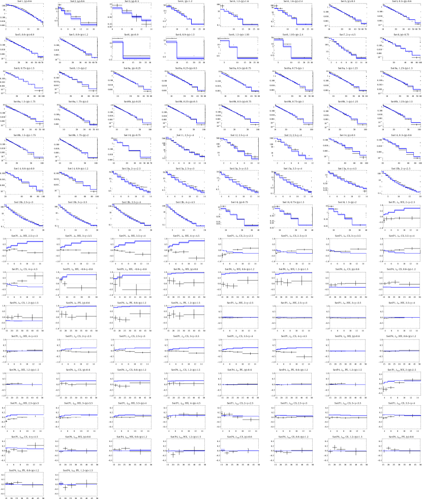
Figure 1: The theoretical results for $d\sigma(p\overset{\text{(}-\text{)}}{p}\to\psi(2S)+X)/dp_{T}$ [nb/GeV], $\lambda_{\theta}$, $\lambda_{\phi}$, and $\lambda_{\theta\phi}$ as functions of $p_{T}$ [GeV] evaluated using the results of fit A (blue) are compared to the data in Table 1 (black). All the shown data is fitted to. The errors bands indicate the scale uncertainties as described in the text.

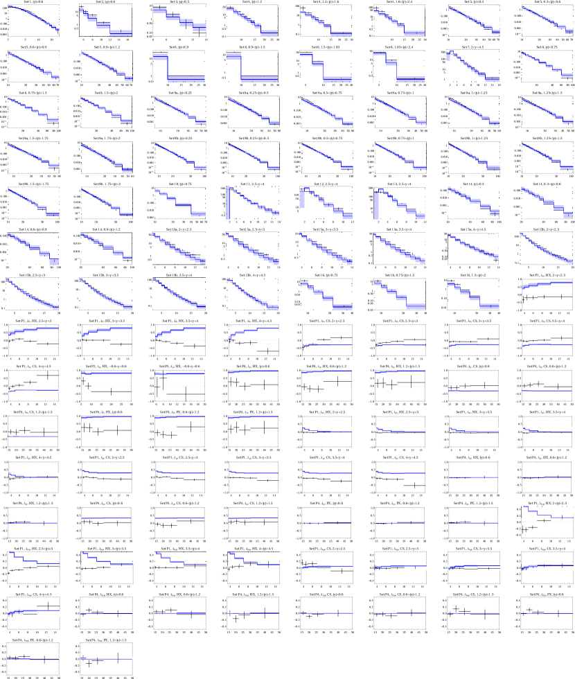
Figure 2: As in Fig. 1, but for fit B. Only the unpolarized data (sets 1–16) is fitted to.

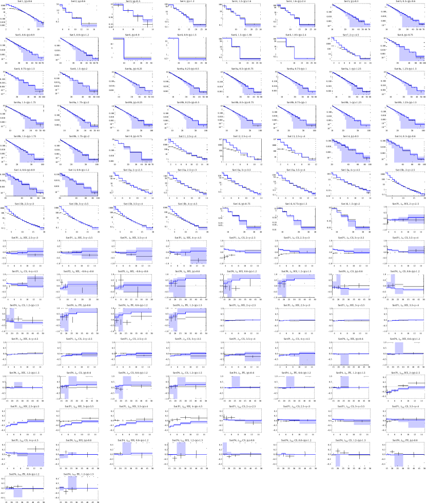
Figure 3: As in Fig. 1, but for fit C. Only the data with $p_{T}>7$ GeV is fitted to.

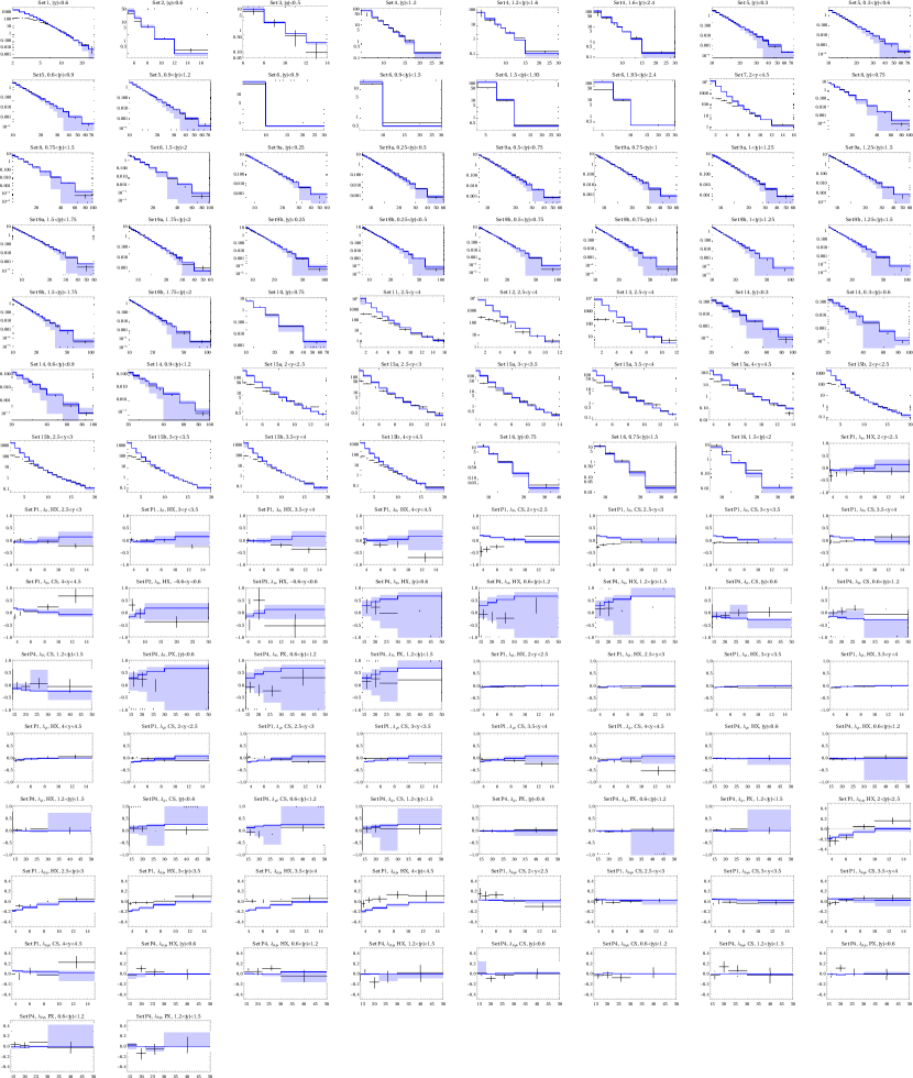
Figure 4: As in Fig. 1, but for fit D. Only the unpolarized data (sets 1–16) with $p_{T}>7$ GeV is fitted to.

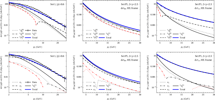
Figure 5: The theoretical results for $d\sigma/dp_{T}$ appropriate for set 1 Aaltonen:2009dm (left column), $d\sigma_{00}/dp_{T}$ (center column), and $d\sigma_{11}/dp_{T}$ (right column) in the HX frame appropriate for the first $y$ bin of set P1 Aaij:2014qea , evaluated using the results of fit A, are broken down to their CS contributions and their CO contributions proportional to $O_{i}$ in Eq. (4) (upper row) and $V_{i}$ in Eq. (9) (lower row). Red color indicates negative values. The data of set 1 are shown for comparison.

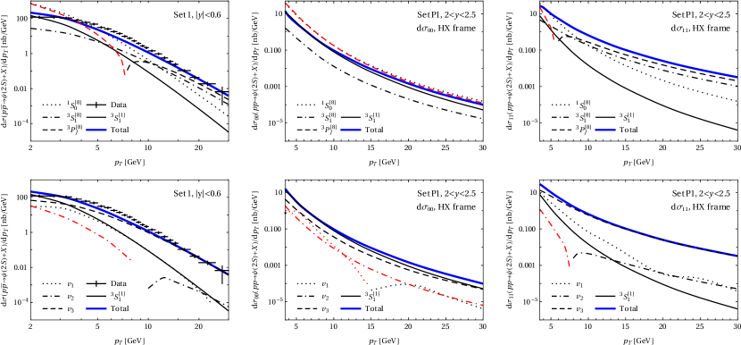
Figure 6: Same as in Fig. 5, but for fit B.

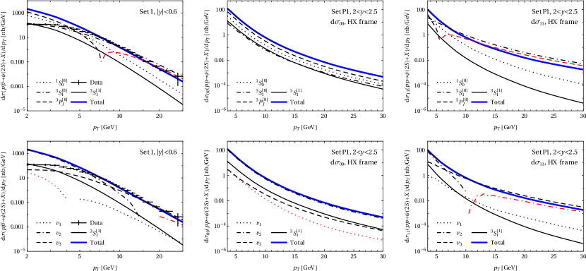
Figure 7: Same as in Fig. 5, but for fit C.

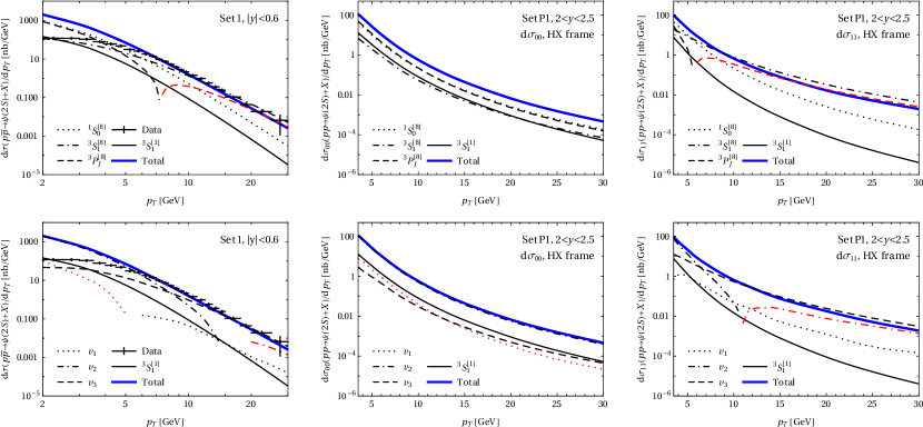
Figure 8: Same as in Fig. 5, but for fit D.

V Summary

To summarize, working at NLO in $\alpha_{s}$ within the NRQCD factorization framework Bodwin:1994jh , we have fitted the three CO LDMEs of the $\psi(2S)$ meson leading in $v$, $\langle{\cal O}^{\psi(2S)}({{}^{1}S}_{0}^{[8]})\rangle$, $\langle{\cal O}^{\psi(2S)}({{}^{3}S}_{1}^{[8]})\rangle$, and $\langle{\cal O}^{\psi(2S)}({{}^{3}P}_{0}^{[8]})\rangle$, to the world data of single $\psi(2S)$ inclusive hadroproduction, both unpolarized and polarized (see Table 1). We have independently applied two filters to the experimental data, excluding data with $p_{T}<7$ GeV and/or polarization, yielding four independent fits, labeled A–D. Our fit results are collected in Table 2. They are all compatible with the velocity scaling rules of NRQCD Lepage:1992tx . We find that the polarization data has limited effect on the fit results, while a consistent description of all data is infeasible without a large low-$p_{T}$ cut, such as $p_{T}>7$ GeV, which reduces $\chi^{2}/\mathrm{d.o.f.}$ by more than a factor of 5, down to 2.7 and 2.5, leading to reasonably good overall descriptions of the data. Thanks to the greatly enlarged data sample used, the results of our fits with $p_{T}>7$ GeV are one order of magnitude more precise than those of the previous fit in Refs. Ma:2010yw ; Ma:2010jj , which is otherwise similar to ours. This has even allowed us to pin down, with an uncertainty of about 40%, a third linear combination of LDMEs, which has so far been out of reach. However, the increased precision of the fits with $p_{T}>7$ GeV comes at the expense of reduced perturbative stability over wide kinematic ranges, manifesting itself as high sensitivity to scale variations.

At this point, one may ask how far NRQCD factorization is consolidated or challenged in view of the advanced precision of our global analysis of single $\psi(2S)$ inclusive hadroproduction. Unfortunately, the answer to this question is somewhat ambiguous. While fixed-order perturbation theory, as employed here, is expected to break down in the limit $p_{T}\to 0$ due the appearance of large soft-gluon logarithms requiring resummation, it is unclear why a small-$p_{T}$ cutoff as large as $p_{T}^{\mathrm{cutoff}}\approx 2M_{\psi(2S)}$ should be necessary to enable an acceptable global fit. In other words, one would expect smaller cutoff values, $p_{T}^{\mathrm{cutoff}}\lessapprox M_{\psi(2S)}$ say, to also allow for useful global fits, which they do not, as we have seen in fits A and B. On the other hand, more serious challenges for NRQCD factorization might have just not surfaced yet, given that, in want of data, we have been confined to just one inclusive production mode, namely single hadroproduction. This is very different for the $J/\psi$ meson, which has been observed in a variety of alternative inclusive production modes, including single photoproduction Butenschoen:2009zy ; Butenschoen:2011ks , hadroproduction in pairs He:2015qya ; He:2018hwb ; He:2019qqr or in association with a $W$ or $Z$ boson Butenschoen:2022wld . Furthermore, the LDMEs of the $J/\psi$ meson are related by heavy-quark spin symmetry to those of the $\eta_{c}$ meson, which has been observed in single inclusive hadroproduction Butenschoen:2014dra . It will be very interesting to also study such alternative inclusive production modes for the $\psi(2S)$ meson in the future, the more so as feed-down contributions, which complicate the $J/\psi$ case, are practically absent here.

- (1) G. T. Bodwin, E. Braaten, and G. P. Lepage, “Rigorous QCD analysis of inclusive annihilation and production of heavy quarkonium,” Phys. Rev. D 51, 1125–1171 (1995); [Erratum: Phys. Rev. D 55, 5853–5854 (1997)].
- (2) G. P. Lepage, L. Magnea, C. Nakhleh, U. Magnea, and K. Hornbostel, “Improved nonrelativistic QCD for heavy-quark physics,” Phys. Rev. D 46, 4052–4067 (1992).
- (3) Y.-Q. Ma, K. Wang, and K.-T. Chao, “ Production at the Tevatron and LHC at in Nonrelativistic QCD,” Phys. Rev. Lett. 106, 042002 (2011).
- (4) Y.-Q. Ma, K. Wang, and K.-T. Chao, “Complete next-to-leading order calculation of the and production at hadron colliders,” Phys. Rev. D 84, 114001 (2011).
- (5) H.-S. Shao, H. Han, Y.-Q. Ma, C. Meng, Y.-J. Zhang, and K.-T. Chao, “Yields and polarizations of prompt and production in hadronic collisions,” JHEP 05, 103 (2015).
- (6) T. Aaltonen et al. (CDF Collaboration), “Production of mesons in collisions at 1.96 TeV,” Phys. Rev. D 80, 031103(R) (2009).
- (7) B. Gong, L.-P. Wan, J.-X. Wang, and H.-F. Zhang, “Polarization for Prompt and Production at the Tevatron and LHC,” Phys. Rev. Lett. 110, 042002 (2013).
- (8) R. Aaij et al. (LHCb Collaboration), “Measurement of meson production in collisions at TeV,” Eur. Phys. J. C 72, 2100 (2012) [Erratum: Eur. Phys. J. C 80, 49 (2020)].
- (9) G. T. Bodwin, K.-T. Chao, H. S. Chung, U-R. Kim, J. Lee, and Y.-Q. Ma, “Fragmentation contributions to hadroproduction of prompt , , and states,” Phys. Rev. D 93, 034041 (2016).
- (10) S. Chatrchyan et al. (CMS Collaboration), “ and production in collisions at TeV,” JHEP 02, 011 (2012).
- (11) V. Khachatryan et al. (CMS Collaboration), “Measurement of and Prompt Double-Differential Cross Sections in Collisions at TeV,” Phys. Rev. Lett. 114, 191802 (2015).
- (12) N. Brambilla, H. S. Chung, A. Vairo, and X.-P. Wang, “Production and polarization of -wave quarkonia in potential nonrelativistic QCD,” Phys. Rev. D 105, L111503 (2022).
- (13) N. Brambilla, A. Pineda, J. Soto, and A. Vairo, “Potential NRQCD: an effective theory for heavy quarkonium,” Nucl. Phys. B 566, 275–310 (2000).
- (14) G. Aad et al. (ATLAS Collaboration), “Measurement of upsilon production in 7 TeV collisions at ATLAS,” Phys. Rev. D 87, 052004 (2013).
- (15) M. Butenschön and B. A. Kniehl, “Reconciling production at HERA, RHIC, Tevatron, and LHC with Nonrelativistic QCD Factorization at Next-to-Leading Order,” Phys. Rev. Lett. 106, 022003 (2011).
- (16) M. Butenschoen and B. A. Kniehl, “ Polarization at the Tevatron and the LHC: Nonrelativistic-QCD Factorization at the Crossroads,” Phys. Rev. Lett. 108, 172002 (2012).
- (17) M. Butenschoen and B. A. Kniehl, “Dipole subtraction at next-to-leading order in nonrelativistic-QCD factorization,” Nucl. Phys. B 950, 114843 (2020).
- (18) M. Butenschoen and B. A. Kniehl, “Dipole subtraction vs. phase space slicing in NLO NRQCD heavy-quarkonium production calculations,” Nucl. Phys. B 957, 115056 (2020).
- (19) E. J. Eichten and C. Quigg, “Quarkonium wave functions at the origin,” Phys. Rev. D 52, 1726–1728 (1995).
- (20) W. Buchmuller and S.-H. H. Tye, “Quarkonia and quantum chromodynamics,” Phys. Rev. D 24, 132–156 (1981).
- (21) S. Dulat, T.-J. Hou, J. Gao, M. Guzzi, J. Huston, P. Nadolsky, J. Pumplin, C. Schmidt, D. Stump, and C.-P. Yuan, “New parton distribution functions from a global analysis of quantum chromodynamics,” Phys. Rev. D 93, 033006 (2016).
- (22) A. Buckley, J. Ferrando, S. Lloyd, K. Nordström, B. Page, M. Rüfenacht, M. Schönherr, and G. Watt, “LHAPDF6: parton density access in the LHC precision era,” Eur. Phys. J. C 75, 132 (2015).
- (23) P. A. Zyla et al. (Particle Data Group), “Review of Particle Physics,” Prog. Theor. Exp. Phys. 2020, 083C01 (2020).
- (24) S. Chekanov et al. (ZEUS Collaboration), “Measurements of inelastic and photoproduction at HERA,” Eur. Phys. J. C 27, 173–188 (2003).
- (25) F. Abe et al. (CDF Collaboration), “ and Production in Collisions at TeV,” Phys. Rev. Lett. 79, 572–577 (1997).
- (26) F. Abe et al. (CDF Collaboration), “Inclusive , , and -Quark Production in Collisions at TeV,” Phys. Rev. Lett. 69, 3704–3708 (1992).
- (27) A. M. Sirunyan et al. (CMS Collaboration), “Measurement of prompt production cross sections in proton-lead and proton-proton collisions at TeV,” Phys. Lett. B 790, 509–532 (2019).
- (28) G. Aad et al. (ATLAS Collaboration), “Measurement of the production cross-section of in collisions at TeV at ATLAS,” JHEP 09, 079 (2014).
- (29) G. Aad et al. (ATLAS Collaboration), “Measurement of the differential cross-sections of prompt and non-prompt production of and in collisions at and 8 TeV with the ATLAS detector,” Eur. Phys. J. C 76, 283 (2016).
- (30) M. Aaboud et al. (ATLAS Collaboration), “Measurements of and production in collisions at TeV with the ATLAS detector,” JHEP 01, 117 (2017).
- (31) S. Acharya et al. (ALICE Collaboration), “Energy dependence of forward-rapidity and production in collisions at the LHC,” Eur. Phys. J. C 77, 392 (2017).
- (32) B. Abelev et al. (ALICE Collaboration), “Measurement of quarkonium production at forward rapidity in collisions at TeV,” Eur. Phys. J. C 74, 2974 (2014).
- (33) J. Adam et al. (ALICE Collaboration), “Inclusive quarkonium production at forward rapidity in collisions at TeV,” Eur. Phys. J. C 76, 184 (2016).
- (34) A. M. Sirunyan et al. (CMS Collaboration), “Measurement of quarkonium production cross sections in collisions at TeV,” Phys. Lett. B 780, 251–272 (2018).
- (35) R. Aaij et al. (LHCb Collaboration), “Measurement of production cross-sections in proton-proton collisions at and 13 TeV,” Eur. Phys. J. C 80, 185 (2020).
- (36) M. Aaboud et al. (ATLAS Collaboration), “Measurement of quarkonium production in proton–lead and proton–proton collisions at with the ATLAS detector,” Eur. Phys. J. C 78, 171 (2018).
- (37) R. Aaij et al. (LHCb Collaboration), “Measurement of polarisation in collisions at TeV,” Eur. Phys. J. C 74, 2872 (2014).
- (38) A. Abulencia et al. (CDF Collaboration), “Polarization of and Mesons Produced in Collisions at TeV,” Phys. Rev. Lett. 99, 132001 (2007).
- (39) T. Affolder et al. (CDF Collaboration), “Measurement of and Polarization in Collisions at TeV,” Phys. Rev. Lett. 85, 2886–2891 (2000).
- (40) S. Chatrchyan et al. (CMS Collaboration), “Measurement of the prompt and polarizations in collisions at TeV,” Phys. Lett. B 727, 381–402 (2013).
- (41) M. Butenschön and B. A. Kniehl, “Complete Next-to-Leading-Order Corrections to Photoproduction in Nonrelativistic Quantum Chromodynamics,” Phys. Rev. Lett. 104, 072001 (2010).
- (42) M. Butenschoen and B. A. Kniehl, “Probing Nonrelativistic QCD Factorization in Polarized Photoproduction at Next-to-Leading Order,” Phys. Rev. Lett. 107, 232001 (2011).
- (43) Z.-G. He and B. A. Kniehl, “Complete Nonrelativistic-QCD Prediction for Prompt Double Hadroproduction,” Phys. Rev. Lett. 115, 022002 (2015).
- (44) Z.-G. He, B. A. Kniehl, and X.-P. Wang, “Breakdown of Nonrelativistic QCD Factorization in Processes Involving Two Quarkonia and its Cure,” Phys. Rev. Lett. 121, 172001 (2018).
- (45) Z.-G. He, B. A. Kniehl, M. A. Nefedov, and V. A. Saleev, “Double Prompt Hadroproduction in the Parton Reggeization Approach with High-Energy Resummation,” Phys. Rev. Lett. 123, 162002 (2019).
- (46) M. Butenschoen and B. A. Kniehl, “New constraints on NRQCD long-distance matrix elements from plus production at the CERN LHC,” [arXiv:2207.09366 [hep-ph]].
- (47) M. Butenschoen, Z.-G. He, and B. A. Kniehl, “ Production at the LHC Challenges Nonrelativistic QCD Factorization,” Phys. Rev. Lett. 114, 092004 (2015).