Accommodating false positives within acoustic spatial capture-recapture, with variable source levels, noisy bearings and an inhomogeneous spatial density

Abstract

Passive acoustic monitoring is a promising method for surveying wildlife populations that are easier to detect acoustically than visually. When animal vocalisations can be uniquely identified on an array of sensors, the potential exists to estimate population density through acoustic spatial capture-recapture (ASCR). However, sound classification is imperfect, and in some situations a high proportion of sounds detected on just a single sensor (‘singletons’) are not from the target species. We present a case study of bowhead whale calls (Baleana mysticetus) collected in the Beaufort Sea in 2010 containing such false positives. We propose a novel extension of ASCR that is robust to false positives by truncating singletons and conditioning on calls being detected by at least two sensors. We allow for individual-level detection heterogeneity through modelling a variable sound source level, model inhomogeneous call spatial density, and include bearings with varying measurement error. We show via simulation that the method produces near-unbiased estimates when correctly specified. Ignoring source level variation resulted in a strong negative bias, while ignoring inhomogeneous density resulted in severe positive bias. The case study analysis indicated a band of higher call density approximately 30km from shore; 59.8% of singletons were estimated to have been false positives.

Supplementary materials accompanying this paper appear online.

Keywords— bioacoustics, bowhead whale, estimating animal abundance, passive acoustic density estimation, spatially explicit capture recapture, wildlife population assessment

1 Introduction

In recent decades, passive acoustic monitoring (PAM) has increasingly been used to study both terrestrial (Sugai et al., 2019) and marine animals, particularly cetaceans (Zimmer, 2011). Compared with more traditional visual survey methods, acoustic monitoring works day and night, is robust to variation in environmental conditions such as weather, and in some habitats has the potential to detect animals at greater distances, hence increasing the area surveyed (Marques et al., 2011). It has enabled studies of rare and elusive species such as the vaquita (Thomas et al., 2017) and several species of beaked whale (Hildebrand et al., 2015; Yack et al., 2013) which, despite being visually cryptic, produce frequent sounds that can be detected by PAM systems.

One important application of PAM is to estimate population density or abundance (Marques et al., 2013). In the situation where multiple acoustic sensors are deployed simultaneously with a spatial separation such that some vocalisations can be detected on multiple sensors then an appropriate statistical framework for estimating density is spatial capture-recapture (SCR; also known as spatially explicit capture-recapture) (e.g., Borchers et al., 2015; Stevenson et al., 2015). SCR is an extension of long-established capture-recapture (otherwise known as mark-recapture or mark-resight) methods where data on the detection (‘capture’) of individually-identified animals is supplemented by data on the spatial location of the survey effort and the detections (Borchers and Efford, 2008; Royle et al., 2009; Kidney et al., 2016). Recording not just whether but also where each animal was detected increases the accuracy of abundance and density estimates and potentially allows estimation of a spatially inhomogeneous animal density surface.

Acoustic spatial capture-recapture (ASCR) is a special case of SCR where the detections are of individual animal vocalisations or ‘cues’. Standard SCR relies on animals moving between detection locations and hence typically requires multiple capture occasions, while in ASCR the sound travels almost instantaneously from its source and hence can be detected on multiple sensors in a single occasion. Estimation is of cue spatial density; to convert to animal density an estimate of average cue production rate is required (Marques et al., 2013; Stevenson et al., 2021). As well as the location of detection, additional information is often available about the location of the vocalisation, e.g., the bearing, received sound level or time of arrival on multiple sensors. Borchers et al., (2015) showed that using this additional information further improved estimation accuracy.

PAM data can also present challenges that require accounting for to avoid bias in ASCR analysis. First, sound classification is imperfect, leading to false positive detections of sounds not originating from the target species. Second, vocalisation source level can vary considerably, causing heterogeneity in detectability. Third, there can be considerable measurement error in the additional information, particularly the bearings. Forth (in common with other SCR studies), spatial density of source locations can vary substantially.

The methods presented here are motivated by a case study that demonstrates all four of the above issues: estimation of call density of bowhead whales (Baleana mysticetus) migrating through the Beaufort Sea. Multiple arrays of acoustic sensors were deployed in the Beaufort Sea during the migration season and recorded millions of bowhead whale calls. Automated detection and classification methods were therefore used to process the data, yielding call detections, received sound levels and bearings, and linking calls across detectors. However, a high proportion of the detections made on only one sensor (‘singletons’) were thought to be false positives. Naively including these singletons in the analysis would lead to a positive bias in the estimated abundance of unknown but likely substantial magnitude. To avoid this, we excluded all singletons from the analysis and conditioned the ASCR likelihood to only include calls detected on multiple sensors (‘multiply-detected calls’). Truncating the data in this manner, rather than attempting to model the proportion of false positives, is a good strategy when data are plentiful (see Discussion). Conn et al., (2011) proposed a similar procedure in a mark-resight study as a way to differentiate between resident and transient bottlenose dolphin populations, assuming that transients were never detected more than once. To our knowledge, this is the first time this approach has been used in SCR.

Our case study features some additional complications that may commonly appear in real-world data but are not typically all dealt with. Call source level was thought to vary substantially and so we include source level as a random effect in our model. Exploratory analysis showed that, while most estimated bearings were accurate, some appeared to be very inaccurate. We therefore developed a two-part discrete mixture model for bearing error, extending the bearing error methods of Borchers et al., (2015). Finally, we allowed for an inhomogeneous density model to accommodate the spatial preference of the migrating whales (and thus their calls).

In Section 2 we describe the case study in more detail. We then present the extended ASCR model in Section 3. In Section 4 we evaluate the model performance via simulation, and show how ignoring some of the real-world issues can result in substantial bias. Section 5 gives results from a proof-of-concept application of the model to a single day of data. Finally, in Section 6, we discuss results, limitations and alternatives.

2 Case Study

Every year from August to October, the Bering–Chukchi–Beaufort (BCB) population of bowhead whales (Baleana mysticetus) migrates westwards through the Beaufort Sea to their wintering areas in the Bering Sea (Blackwell et al., 2007). They travel mainly over the continental shelf in waters less than 25 meters deep, approximately 10–75 km offshore (Greene et al., 2004). During this migration, bowhead whales are known to produce a wide variety of calls (Ljungblad et al., 1982). The purpose of these calls remains largely unknown, although they may be used for long-range communication (Thode et al., 2020) or to navigate through ice (George et al., 1989).

Between 2007 and 2014, up to 35 Directional Autonomous Seafloor Acoustic Recorders (DASARs; Greene et al., 2004) were deployed at several sites off the north coast of Alaska to monitor the calling behaviours of the migrating whales during seismic surveys. An automated detection and classification procedure was developed to handle the more than one million detected calls over the period 2007–2014 (Thode et al., 2012, 2020). This procedure could identify discrete sounds as bowhead whale calls, and subsequently link them with detections from other DASARs within the array if they were the same call (Thode et al., 2012).

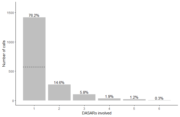
Figure 1: Counts of detected calls by number of DASARs (sensors) involved per call at site 5 on 31 August 2010. Detections were included if the received level was at least 96 dB. The high proportion of singletons (detections on a single DASAR; 1417) raised concerns about the validity of those calls. The dashed line shows the number of singletons (570) that were estimated to be valid using the methods developed in this paper.

Even though it was not the original purpose of the monitoring, the detection and linking of calls created detection histories for every detected call, making these data suitable for ASCR. ASCR theory assumes capture histories without errors, i.e., calls can be missed but not incorrectly positively identified or matched. Several data cleaning procedures were required to meet this assumption as far as possible. Sometimes, calls would be wrongly identified as other discrete sounds. Distant airgun signals were occasionally misidentified as bowhead whale calls; bearded seals (Erignathus barbatus) and walruses (Odobensu rosmarus divergens) could appear similar as well, but these were generally rare and much quieter (Thode et al., 2012). Moreover, if bowhead whale calls overlapped in time, they could be incorrectly matched as being the same call. Cheoo, (2019) showed that the number of detection histories that involved just one sensor (‘singletons’) in the automated data was not in line with expectations based on sound propagation theory (see Figure 1). It was therefore hypothesised that these singletons contain a high-degree of incorrectly classified calls (‘false positives’), mostly consisting of random fluctuations in the noise field or reverberations of whale calls, which were unlikely to be associated among multiple detectors. The solution we present here is to exclude singleton detection histories all together and modify the ASCR likelihood to be conditional on the capture histories involving at least two sensors. To ensure that the multiply-detected calls would contain no false positives, we cleaned the remaining data using a procedure described in Appendix A in Supplementary Materials.

In this study, we focus on the data from one specific day, 31 August 2010, from site 5, the most eastward site, as this site was one of the more intensely studied subsets of the data. Moreover, calls accumulated somewhat evenly across the day, resulting in a low expected rate of overlapping calls. For every call the following data were recorded: a detection history as well as bearings, received sound levels, and noise levels for every involved DASAR. The source level and origin of the call are unobserved, and hence treated as latent variables. Throughout this manuscript, all sound measurements are denoted on the decibel scale (RMS; dB re 1 $\mu$Pa). More details on the background, availability, and pre-processing of the data are presented in Appendix A in Supplementary Materials.

3 Model

In this section, we first introduce the full likelihood. Following that, we derive each element of the likelihood individually. Consider an acoustic survey of an array of $K$ sensors operating within a survey region $\mathcal{A}\subset\mathbb{R}^{2}$ over a period of time $T$. A total of $n$ unique animal calls are detected by at least two sensors. For any multiply-detected call $i\in{1,...,n}$, let $\omega_{ij}$ be 1 if the call was detected at sensor $j\in{1,...,K}$, and $0$ otherwise. We define the matrix containing all detection histories as $\bm{\Omega}=(\bm{\omega}_{1},...,\bm{\omega}_{n})^{\top}$, where the detection history for call $i$ is denoted $\bm{\omega}_{i}=(\omega_{i1},...,\omega_{iK})^{\top}$ and $\top$ denotes the transpose. For every call $i$ that was detected at sensor $j$, we also observe the bearing $y_{ij}$, measured in degrees clockwise relative to true north, and the received sound level $r_{ij}$. These data are contained in $\bm{Y}=(\bm{y}_{1},...,\bm{y}_{n})^{\top}$ and $\bm{R}=(\bm{r}_{1},...,\bm{r}_{n})^{\top}$, respectively. Latent variables are the spatial origins of calls, denoted by $\bm{X}=(\bm{x}_{1},...,\bm{x}_{n})^{\top}$ where $\bm{x}_{i}$ is a location in the Cartesian plane, and the source levels, denoted by $\bm{s}=(s_{1},...,s_{n})^{\top}$. The support for $s$ is denoted $\mathcal{S}$. Throughout this manuscript, we do not distinguish explicitly in notation between random variables and specific observations/realisations – this should be clear from the context.

The parameter vectors used in the model are (following previous literature as closely as possible): $\bm{\phi}$ for parameters associated with the spatial density of emitted calls, $\bm{\nu}$ for those associated with the source levels of calls, $\bm{\eta}$ for those associated with source sound propagation and received levels, $\bm{\theta}$ for those associated with detectability of calls, and $\bm{\gamma}$ for those associated with measurement error of the bearings. For notational convenience we define the joint parameter vector $\bm{\xi}=(\bm{\phi},\bm{\nu},\bm{\eta},\bm{\theta},\bm{\gamma})$. A list of model assumptions is presented in Section 3.10.

3.1 Likelihood Specification

The likelihood is formed from the joint distribution of all observed and latent variables introduced above. We denote this likelihood $\mathcal{L}_{f}(\bm{\xi})$ where the subscript $f$ stands for ‘full’ to distinguish it from the conditional likelihood $\mathcal{L}_{c}(\bm{\xi})$ which is conditional on the observed number of detections. Denoting both probability mass and density functions as $f(.)$, we define the full likelihood as

$$\mathcal{L}_{f}(\bm{\xi}) =f(n,\bm{\Omega},\bm{Y},\bm{R},\bm{X},\bm{s};\bm{\xi})$$ (1)

$$=f(n;\bm{\phi},\bm{\theta},\bm{\nu})\times f(\bm{\Omega},\bm{Y},\bm{R},\bm{X},\bm{s}|n;\bm{\xi})$$

$$=f(n;\bm{\phi},\bm{\theta},\bm{\nu})\times\mathcal{L}_{c}(\bm{\xi}).$$

As we do not observe the call locations and source levels, we marginalise over the unobserved $\bm{X}$ and $\bm{s}$ to obtain

$$\mathcal{L}_{c}(\bm{\xi})= \int_{\mathcal{S}}\int_{\mathcal{A}}f(\bm{\Omega},\bm{Y},\bm{R},\bm{X},\bm{s}|n;\bm{\xi})d\bm{X}d\bm{s}.$$ (2)

The double integral in Equation (2) is of dimension $3n$, making this likelihood intractable. We follow Stevenson et al., (2015) in assuming calls to be independent of each other in all respects, allowing us to specify Equation (2) as the product of $n$ 3-dimensional integrals:

$$\mathcal{L}_{c}(\bm{\xi})\equiv \prod_{i\in\{1:n\}}\int_{\mathcal{S}}\int_{\mathcal{A}}f(\bm{\omega}_{i},\bm{y}_{i},\bm{r}_{i},\bm{x}_{i},s_{i}|\omega_{i}^{*}\geq 2;\bm{\xi})d\bm{x}_{i}ds_{i}$$ (3)

$$= \prod_{i\in\{1:n\}}\int_{\mathcal{S}}\int_{\mathcal{A}}f(\bm{\omega}_{i}|\bm{x}_{i},\bm{s}_{i},\omega_{i}^{*}\geq 2;\bm{\theta})$$

$$\quad\quad\times f(\bm{y}_{i}|\bm{\omega}_{i},\bm{x}_{i};\bm{\gamma})\times f(\bm{r}_{i}|\bm{\omega}_{i},\bm{x}_{i},s_{i};\bm{\eta})$$

$$\quad\quad\times f(\bm{x}_{i}|s_{i},\omega_{i}^{*}\geq 2;\bm{\phi},\bm{\theta})$$

$$\quad\quad\times f(s_{i}|\omega_{i}^{*}\geq 2;\bm{\phi},\bm{\theta},\bm{\nu})d\bm{x}_{i}ds_{i}$$

where we assume independence between $\bm{y}_{i}$ and $\bm{r}_{i}$ given $\bm{x}_{i}$, and $\omega_{i}^{*}:=\sum_{j\in 1:k}w_{ij}$ denotes the total number of sensors involved in the detection of call $i$. The separation of the joint distribution inside the integrals in (3) follows from repeatedly applying Bayes’ formula. Note that conditioning the joint distribution on $n$ in (2) is equivalent to conditioning every marginal distribution on involving at least two sensors in (3); for the second and third element this conditioning is implicit in conditioning on detection history $\bm{\omega}_{i}$. If we were to assume a constant spatial density of calls, it would be sufficient to simply maximise $\mathcal{L}_{c}$, as the parameter estimates from the conditional MLE are identical to those obtained by maximising the full likelihood – a Horvitz Thompson-like estimator could then be used to derive the mean density (Borchers and Efford, 2008). In our case study, however, the spatial density of calls is known to be inhomogeneous, so the full likelihood is required.

In the following sections, we specify in further detail $f(n;\bm{\phi},\bm{\theta},\bm{\nu})$ and the five components in Equation (3). For readability we will hereforth omit the indexing of parameters in the probability functions.

3.2 Detection Probability, $p(\bm{x}_{i},s_{i})$

A fundamental part of ASCR is the concept of a detection probability, which is the probability that an emitted call is detected by a sensor – this is the way ASCR accommodates for missed calls, i.e., false negatives. The function that relates this probability to covariates is called the detection function, denoted $p(.)$. For ASCR it was proposed to be most appropriate to use a detection function based on the received (sound) level, also known as signal strength, which is primarily a function of source level and range (Efford et al., 2009; Stevenson et al., 2015). We propose a detection function for sensor $j$ where $g_{0}\in(0,1)$ denotes the detection probability when the true received level of a call surpasses threshold $t_{r}$, and zero probability else, as follows

$$p_{j}(\bm{x}_{i},s_{i})=g_{0}\times\left(1-\Phi\left(\frac{t_{r}-\mathbb{E}[r_{ij}|\bm{x}_{i},s_{i}])}{\sigma_{r}}\right)\right),$$ (4)

where $\Phi$ denotes the standard normal cumulative density function (cdf) and $\sigma_{r}$ denotes the measurement and propagation error on received level (see Section 3.4). The threshold $t_{r}$ should be set by the analyst, and in this study is roughly equal to the maximum level of ocean background noise. As there is error on the received levels, calls with an expected received level close to $t_{r}$ can have a detection probability between 0 and $g_{0}$.

3.3 Detected Calls, $f(n)$

To construct a probability function for the number of detected calls, we start with the distribution of emitted calls, which are assumed to occur independently of one another in space and time. Thus, let the number of emitted calls at point $\bm{x}$ in period $T$ be a realisation of a spatially-inhomogeneous Poisson point process with intensity $D(\bm{x})$. As we only observe multiply-detected calls, we take the product of this intensity and the probability of multiply detection, denoted by

$$p.(\bm{x}_{i},s_{i}) =\mathbb{P}(\omega^{*}\geq 2|\bm{x}_{i},s_{i})$$ (5)

$$=1-\mathbb{P}(\omega^{*}=0|\bm{x}_{i},s_{i})-\mathbb{P}(\omega^{*}=1|\bm{x}_{i},s_{i}),$$

where $\omega^{*}:=\sum_{j\in{1:k}}\omega_{j}$. Note that Equation (5) is the part of the method that deviates from conventional ASCR and allows us to exclude all singletons. We rewrite Equation (5) and marginalise over source level to get the filtered Poisson point process with spatially varying rate parameter $\int_{\mathcal{S}}D(\bm{x})p.(\bm{x},s)f(s)ds$. Lastly, we marginalise over $\bm{x}$ to get the distribution of the total number of multiply-detected calls over time $T$:

$$n\sim\text{Poisson}\left(\int_{\mathcal{A}}\int_{\mathcal{S}}D(\bm{x})p.(\bm{x},s)f(s)dsd\bm{x}\right).$$ (6)

The expected total number of emitted calls is then derived by integrating the density over the study area, such that $\mathbb{E}[N]=\int_{\mathcal{A}}D(\bm{x})d\bm{x}$.

3.4 Received Level, $f(\bm{r}_{i}|\bm{\omega}_{i},\bm{x}_{i},s_{i};\bm{\eta})$

Sound waves propagating through water lose strength through various mechanisms (Jensen et al., 2011), a process known as ‘transmission loss’. We approximate this process by allowing a single parameter $\beta_{r}$ to determine the acoustic transmission loss, such that

$$\mathbb{E}[r_{ij}|\bm{x}_{i},s_{i}]=s_{i}-\beta_{r}\log_{10}(d_{j}(\bm{x}_{i})),$$ (7)

where $d_{j}(\bm{x}_{i})$ returns the distance from sensor $j$ to location $\bm{x}_{i}$. Here, $\beta_{r}=20$ would reflect purely spherical spreading loss while $\beta_{r}=10$ would reflect cylindrical spreading loss; in reality the dominant process will be range- and depth-dependent, with other factors also playing a role (Jensen et al., 2011). To capture potential error in the propagation model and the measurement of received level, we follow Stevenson et al., (2015) and assume Gaussian error on the received levels, giving

$$r_{ij}|\bm{x}_{i},s_{i}\sim\mathcal{N}\left(\mathbb{E}[r_{ij}|\bm{x}_{i},s_{i}],\sigma_{r}^{2}\right)$$ (8)

where $\mathcal{N}\left(\mu,\sigma^{2}\right)$ denotes a normal distribution with mean $\mu$ and variance $\sigma^{2}$. Unlike Stevenson et al., (2015), we do not assume all calls above threshold $t_{r}$ to be detected with certainty. Instead, we allow for a single detection probability for calls with received levels above the threshold, since the signal processing used in our case study meant that other factors also determined detectability (see Section 3.2). As $r_{ij}$ is only recorded if sensor $j$ detected the call, we condition the indexing on the $j^{\text{th}}$ DASAR detecting the call. Assuming independence between the sensors, the third component of Equation (3) becomes

$$f(\bm{r}_{i}|\bm{\omega}_{i},\bm{x}_{i},s_{i};\bm{\eta})=$$ (9)

$$\quad\quad\prod_{j\in\{1:K|\omega_{ij}=1\}}\frac{1}{\sigma_{r}}\frac{\phi\left((r_{ij}-\mathbb{E}[r_{ij}|\bm{x}_{i},s_{i}])/\sigma_{r}\right)}{1-\Phi(({t_{r}-\mathbb{E}[r_{ij}|\bm{x}_{i},s_{i}]})/{\sigma_{r}})},$$

where $\phi$ denotes the standard normal probability density function (pdf). This is in effect a normal distribution truncated at $t_{r}$.

3.5 Bearings, $f(\bm{y}_{i}|\bm{\omega}_{i},\bm{x}_{i};\bm{\gamma})$

DASARs were designed to record the direction to discrete sounds; these recorded bearings contain measurement errors. Following Stevenson et al., (2015) and Borchers et al., (2015), we capture this error by assuming a Von Mises distribution with concentration parameter $\kappa$ on the bearings. Analogous to the received levels, we only record bearings at DASARs that detected a call. Assuming that the sensors are independent of each other, the second component of Equation (3) would therefore be

$$f(\bm{y}_{i}|\bm{\omega}_{i},\bm{x}_{i};\bm{\gamma})=$$ (10)

$$\quad\quad\sum_{j\in\{1:K|w_{ij}=1\}}\frac{\exp\{\kappa\cos(y_{ij}-\mathbb{E}[y_{ij}|\bm{x}_{i}])\}}{2\pi I_{0}(\kappa)},$$

with $I_{0}$ denoting the modified Bessel function of degree 0. Exploratory research found that, while most bearings appeared relatively accurate, a small proportion seemed highly inaccurate, and we hence apply a 2-part discrete mixture model on the bearings. In effect, we fit a Von Mises distribution with a lower accuracy (dispersion is $\kappa$) for some proportion of the bearings, $\psi_{\kappa}$, and a Von Mises distribution with higher accuracy (dispersion is $\kappa+\delta_{\kappa}$, where increment $\delta_{\kappa}$ is non-negative) to the remaining proportion of the bearings, $1-\psi_{\kappa}$. The second component of Equation (3) thus becomes

$$f(\bm{y}_{i}|\bm{\omega}_{i},\bm{x}_{i};\bm{\gamma})=$$ (11)

$$\quad\quad\sum_{j\in\{1:K|w_{ij}=1\}}\psi_{\kappa}\frac{\exp\{\kappa\cos(y_{ij}-\mathbb{E}[y_{ij}|\bm{x}_{i}])\}}{2\pi I_{0}(\kappa)}$$

$$\quad\quad\quad\quad\quad\times(1-\psi_{\kappa})\frac{\exp\{(\kappa+\delta_{\kappa})\cos(y_{ij}-\mathbb{E}[y_{ij}|\bm{x}_{i}])\}}{2\pi I_{0}(\kappa+\delta_{\kappa})}.$$

3.6 Call location given $s$ and at least two detections, $f(\bm{x}_{i}|s_{i},\omega^{*}_{i}\geq 2{\color[rgb]{0,0,0};\bm{\phi},\bm{\theta}})$

To evaluate the pdf of call locations, we assume independence between call locations and source levels, and use Bayes’ formula to obtain

$$f(\bm{x}_{i}|s_{i},\omega^{*}_{i}\geq 2{\color[rgb]{0,0,0};\bm{\phi},\bm{\theta}})= \frac{f(\omega^{*}_{i}\geq 2|\bm{x}_{i},s_{i})f(\bm{x}_{i}|s_{i})}{\int_{\mathcal{A}}f(\omega^{*}_{i}\geq 2|\bm{x},s_{i})f(\bm{x}|s_{i})d\bm{x}}$$ (12)

$$= \frac{p.(\bm{x}_{i},s_{i})f(\bm{x}_{i})}{\int_{\mathcal{A}}p.(\bm{x},s_{i})f(\bm{x})d\bm{x}}.$$

Although $f(\bm{x}_{i})$ is unknown, we do know that it is proportional to the emitted call density, such that $f(\bm{x}_{i})={D(\bm{x}_{i})}/{\int_{\mathcal{A}}D(\bm{x})d\bm{x}}$. Thus we can simplify Equation (12) as

$$f(\bm{x}_{i}|s_{i},\omega^{*}_{i}\geq 2{\color[rgb]{0,0,0};\bm{\phi},\bm{\theta}})= \frac{p.(\bm{x}_{i},s_{i}){D(\bm{x}_{i})}/{\int_{\mathcal{A}}D(\bm{x})d\bm{x}}}{\int_{\mathcal{A}}p.(\bm{x},s_{i}){D(\bm{x})}/{\int_{\mathcal{A}}D(\bm{q})d\bm{q}}d\bm{x}}$$ (13)

$$= \frac{p.(\bm{x}_{i},s_{i})D(\bm{x}_{i})}{\int_{\mathcal{A}}p.(\bm{x},s_{i})D(\bm{x})d\bm{x}}.$$

3.7 Source level given at least two detections, $f(s_{i}|\omega^{*}_{i}\geq 2{\color[rgb]{0,0,0};\bm{\phi},\bm{\theta},\bm{\nu}})$

Analogous to above, we assume independence between and among call locations and source levels, to derive

$$f(s_{i}|\omega^{*}_{i}\geq 2{\color[rgb]{0,0,0};\bm{\phi},\bm{\theta},\bm{\nu}})= \frac{f(\omega^{*}_{i}\geq 2|s_{i})f(s_{i})}{f(\omega^{*}_{i}\geq 2)}$$ (14)

$$= \frac{\int_{\mathcal{A}}p.(\bm{x},s_{i})D(\bm{x})d\bm{x}\times f(s_{i})}{\int_{\mathcal{A}}\int_{\mathcal{S}}p.(\bm{x},s)f(s)D(\bm{x})dsd\bm{x}}.$$

Note that a part of the numerator in Equation (14) cancels out against the denominator in Equation (13), and that the denominator of Equation (14) denotes the effective sampled area. Thode et al., (2020) estimated source levels using the estimated origin of the call, the received level on the sensor nearest the origin, and a transmission loss parameter $\beta_{r}$ of 15. Based on the observed distribution of these estimated source levels, we assume a normal distribution on $s_{i}$ truncated at 0, such that

$$s\sim\mathcal{N}_{0}^{\infty}(\mu_{s},\sigma_{s}^{2}).$$ (15)

3.8 Detection History, $f(\bm{\omega}_{i}|\bm{x}_{i},s_{i},\omega^{*}_{i}\geq 2;\bm{\theta})$

If we assume sensors to be independent, we can view the detection history of a call as a realisation of a binomial process with size $K$ and non-constant probability $p_{j}$ with $j=1,..,K$, where the order is relevant and hence the binomial coefficient is absent. This gives

$$f(\bm{\omega}_{i}|\bm{x}_{i},s_{i},\omega^{*}_{i}\geq 2;\bm{\theta})=\frac{\prod^{K}_{j=1}{p_{j}(\bm{x}_{i},s_{i})^{\omega_{ij}}(1-p_{j}(\bm{x}_{i},s_{i}))^{1-\omega_{ij}}}}{p.(\bm{x}_{i},s_{i})},$$ (16)

where $p.(\bm{x}_{i},s_{i})$ appears in the denominator to account for the conditioning on at least two sensors in every call detection history (see Equation (5)).

3.9 Variance Estimation

We do not use the Hessian matrix to extract standard errors, as these are only asymptotically normal. Instead, we estimate uncertainty using a non-parametric bootstrap, where we re-sample the calls with replacement (Borchers et al., 2002) and fit the model every time. Following that, we estimate the standard error by taking the standard deviation of all bootstrapped parameter estimates, and we take the 2.5% and 97.5% percentiles to estimate their 95% confidence intervals.

3.10 Assumptions

The method presented in this manuscript relies on several assumptions, as follows. 1) Call origins are a realisation of a Poisson point process, thus calls are spatially and temporally independent given this process. 2) Calls are omnidirectional and equally detectable given only the received level (i.e., no unmodelled heterogeneity). 3) Sensors are identical in performance and operate independently; 4) Calls are matched without error and identified correctly, but can be missed (i.e., no false positive, but false negatives are allowed). 5) The transmission loss model is correctly specified. 6) Uncertainty on bearings and received levels are independent. 7) Source level of a call is independent of space and time. These assumptions are discussed in more detail in Appendix B in Supplementary Materials.

3.11 Practical Implementation

We fitted the model using maximum likelihood estimation (MLE) in R 4.1.0 (R Core Team, 2021) with some components written in C++ and linked to R through the Rcpp library (Eddelbuettel, 2013). We standardised the covariates in the density model to improve the convergence. The estimates were found through optimisation with the function nlminb() (R Core Team, 2021). We used a spatial mesh with non-uniform grid spacing to reduce run-time, with increased grid spacing farther from the sensor array (see Appendix C in Supplementary Materials for details).

4 Simulation Study

We used simulations to evaluate the performance of the model under variable source levels (scenario 1) and fixed source levels (scenario 2). Both scenarios featured measurement error on bearings simulated from a two-part mixture model, and inhomogeneous call density specified as follows:

$$\log(D)=\beta_{0}+\beta_{1}d+\beta_{2}d^{2},$$ (17)

where $d$ denotes the (scaled) shortest distance to the coast. The parameter values used were chosen to match those from the case study data analysis and are given in Table 1.

For each scenario, we simulated 100 data sets and analysed each data set with 5 models: (a) the true model, i.e., that corresponding to the simulated scenario; (b) a model with incorrect assumption about source level, i.e., for scenario 1 the model assumed fixed source level and for scenario 2 the model assumed variable source level; (c) a simpler bearing model assuming a von Mises distribution on bearing error but no two-part mixture; (d) a model that omitted the bearing information altogether; and (e) a model assuming a homogeneous spatial density. We did not include a simulation scenario where we naively fit model to false positives, as the effect on the estimates is already known: it will induce a positive bias that will increase with increasing false positive rate.

For each scenario and model combination (1a-e and 2a-e) we evaluated performance by calculating the coefficient of variation (CV), relative error and relative bias in estimated total abundance. Further details are given in Appendix D in Supplementary Materials.

Parameters	Variable SL	Constant SL
$g_{0}$	0.6	0.6
$\beta_{r}$	18.0	14.5
$\sigma_{r}$	2.7	4.5
$\mu_{s}$	163.0	155.0
$\sigma_{s}$	5.0	-
$\kappa$	0.3	0.3
$\delta_{\kappa}$	36.7	34.7
$\psi_{\kappa}$	0.1	0.1
$\beta_{0}$	-12.0	-16.0
$\beta_{1}$	45.0	57.0
$\beta_{2}$	-53.0	-68.5

Table 1: The parameter values used for the simulation study. These were based on initial fits to the real data, in order to keep the simulations as realistic as possible.

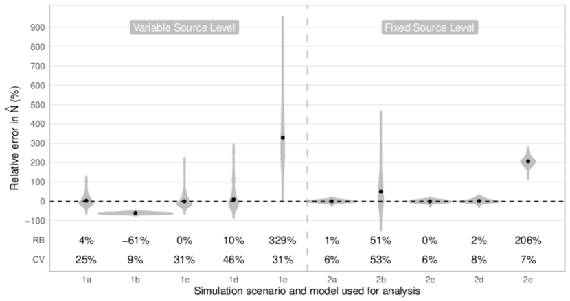
Figure 2: Relative error, relative bias and coefficient of variation for $\hat{N}$ from 100 simulations. The black dots correspond to the relative bias (RB; the mean relative error) and the grey shading shows the spread of relative error per scenario. The RB and coefficient of variation (CV) for every scenario and model combination is shown just above the x-axis. Simulation scenario 1 is variable sound source level and 2 is fixed sound source level. Analysis model (a) is the true model, (b) the incorrect source level model, (c) an incorrect simple bearing model, (d) a model with bearing data, and (e) an incorrect homogeneous spatial density model.

4.1 Results

Both correctly specified models (1a and 2a) gave near-unbiased results (Figure 2). Fitting a single source level model in the variable source level scenario (1b) introduced a strong negative bias with low variance; fitting a variable source level in the fixed source level scenario (2b) introduced a strong negative bias, although this bias could be explained by a flat likelihood surface and resulting sensitivity to starting values. Using an incorrect, simple bearing model (1c and 2c) did not induce bias but did increase variance. Ignoring the bearing information induced a small positive bias and greater variance in the variable source level scenario (1d) but had little effect on the fixed source level scenario (2d). Lastly, using an incorrectly specified constant spatial density model (1e and 2e) resulted in severe overestimation of abundance ($>300\%$ and $>200\%$ bias for variable and fixed source level scenarios, respectively).

5 Bowhead Whale Analysis

We used the proposed method to estimate bowhead whale call density and abundance at site 5 on 31 August 2010. We used data from a single day, and as we present our estimate as call density per day, we did not need to adjust for our study time ($T=1$). We set $t_{r}$ at 96 dB, as the observed background noise never surpassed this level. The true call density surface is unknown and therefore we fitted several candidate models, which we compared using Akaike’s information criterion (AIC; Akaike, (1998)). As the bowhead whales are thought to exhibit a spatial preference based on their distance from the coast and ocean depth during fall migration (Greene et al., 2004), we fitted a canditate set of 35 models containing combinations of distance and depth as linear, quadratic or smooth covariates – see Appendix E in Supplementary Materials for full details. Measures of uncertainty in abundance (standard error, CV, and quantile coefficient of dispersion (QCD)) were derived by bootstrapping the calls 999 times, refitting the AIC-best model each time. The QCD is a relative measure and insensitive to outliers, and is defined as $(Q_{3}-Q_{1})/(Q_{3}+Q_{1})$, where $Q_{1}$ and $Q_{3}$ are the first and third quartile, respectively. To further illustrate the potential benefits of modelling source level heterogeneity, we included point estimates of the best model equivalent with a fixed source level.

5.1 Results

The lowest AIC model included density modelled as a smooth function distance to coast and a quadratic relation with depth. We observe an increase in density, followed by a decrease, as we increase the distance from the coast (Figure 3, left panel). Moreover, density is higher just east of the sensor array, potentially due to some effect of ocean depth. Even though we observe increases in uncertainty in the southern regions and slightly in the north, overall QCD estimates are low (Figure 3, right panel). Total abundance of bowhead whale calls was estimated at 5741 in the study area, and the CVs of the parameter estimates varied considerably, ranging from 0.95% for $\hat{\mu}_{s}$ to 58.22% for $\widehat{\beta_{\text{s(depth).3}}}$ (Table 2).

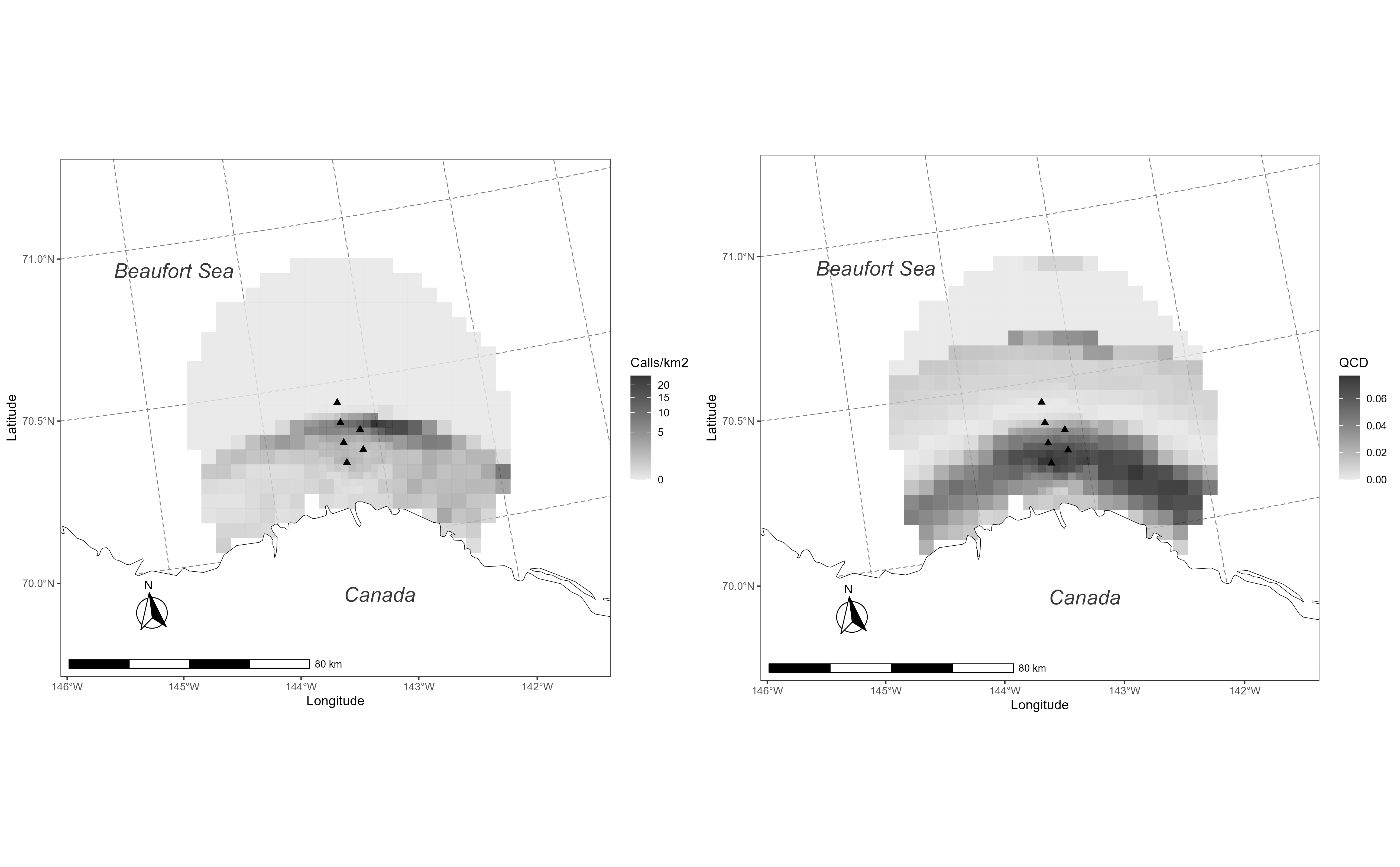
Figure 3: A map of the study site 5 from 31 August 2010 with the estimated density surface (left) and the associated empirical quartile coefficient of dispersion (QCD; right). Locations of the 6 DASARs are indicated with the triangles. The square grid cells within 10 km of the array each have an area of 6.25 km², and and area of 25 km² elsewhere. The density map corresponds to the model with the lowest AIC, which is model 33 in Appendix D in Supplementary Materials. The QCD is derived from 999 Monte Carlo simulations based on the same model, where the calls are re-sampled.

Quantity	Estimate	SE	CV (%)	Single SL
$N$	5741.39	576.01	10.55	1916.06
$g_{0}$	0.55	0.02	2.73	0.67
$\beta_{r}$	17.05	0.33	1.91	13.86
$\sigma_{r}$	2.75	0.11	4.06	4.64
$\mu_{s}$	158.46	1.50	0.95	151.04
$\sigma_{s}$	5.47	0.26	4.90	-
$\kappa$	0.77	0.17	21.95	0.62
$\delta_{\kappa}$	45.49	3.02	6.54	40.23
$\psi_{\kappa}$	0.12	0.01	10.75	0.09
$\beta_{\text{intercept}}$	-265.65	7.92	2.99	-146.81
$\beta_{\text{s(depth).1}}$	42.43	18.07	45.55	80.65
$\beta_{\text{s(depth).2}}$	302.26	6.72	2.23	8.25
$\beta_{\text{s(depth).3}}$	41.14	22.32	58.22	88.65
$\beta_{\text{s(depth).4}}$	-141.57	6.88	4.89	-8.78
$\beta_{\text{s(depth).5}}$	154.60	6.19	4.01	24.23
$\beta_{\text{s(d2c).1}}$	159.48	4.47	2.82	59.19
$\beta_{\text{s(d2c).2}}$	-449.58	15.55	3.47	-185.40
$\beta_{\text{s(d2c).3}}$	101.06	4.29	4.26	33.88
$\beta_{\text{s(d2c).4}}$	-109.30	5.10	4.69	5.14
$\beta_{\text{s(d2c).5}}$	-224.66	11.13	4.96	-142.24

Table 2: The point estimates and associated uncertainties. SE is standard error, CV stands for coefficient of variation, and Single SL are point estimates from the equivalent model without source level heterogeneity. $N$ is a derived quantity; $g_{0}$ through $\psi_{\kappa}$ are the observation parameters presented on the real scale; and the remainder are the density parameters presented on their log link scale.

6 Discussion

We have developed and tested a novel extension of acoustic spatial capture-recapture by conditioning on a minimum of two detections per individual call. Removing single detections may be necessary when the validity of these calls is challenged, and our simulation study shows that the method gives unbiased results in both variable and single source level scenarios. Even though this model applies to (marine) acoustic data, the extension proposed can be applied to all forms of SCR. Fitting a single source level model to variable source level data, thus ignoring heterogeneity in the detectability of the calls, resulted in severe underestimation of abundance. This represents a cautionary tale for other applications of SCR, both terrestrial and aquatic, when it is hypothesised that there is some random variable affecting individual detectability – it does not have to be something as tangible as a source level. Moreover, we confirmed results from Stevenson et al., (2015) on adding bearing information to a SCR model and found a further increase in precision when allowing for a mixture of ‘good’ and ‘bad’ bearings. Finally, we also confirm that incorrectly assuming a constant call density surface can lead to severe overestimates of the abundance.

The notion that density of bowhead whale(s) (calls) is highest 10–75 km from the coast (Greene et al., 2004) seems to be confirmed by the best model, which finds a density that is highest a bit away from the coast, but not too far. The high call spatial density in the northeastern part of the study area (Figure 3) was unexpected, but could have been a consequence of using only data from one day. This likely strongly violated the Poisson assumption about call spatial location, since whale location is spatially auto-correlated, especially on small time scales (Wursig et al., 1985). Alternatively, it has been hypothesised that the higher estimated density of calls in the east could be due to the directionality of the calls or the effect of water depth on sound propagation (Blackwell et al., 2012). In this study, the authors observed 2.1 times as many calls east of the array as west. Future research could explore whether a more gradual increasing/decreasing density slope is found if more days were included in the analysis, resulting in reduced autocorrelation among the call origins.

The model-based expected number of singletons was 570 whereas there were 1417 observed singletons, which is 149% more than expected and confirmed our suspicions regarding false positives (see Figure 1).

An alternative to truncating singletons would be to retain all data and try to model the occurrence of false positive detections. For example, one could assume that an unknown proportion of detections are false positives and include a parameter for this proportion in an analogous way to the $M_{t,\alpha}$ model presented by Yoshizaki, (2007). Detection at any detector $j$ could have three outcomes: no detection with probability $1-p_{j}$, false detection with probability $\alpha p_{j}$, and correct detection with probability $p_{j}$. Moreover, we would have to implement some modification of the $M_{b}$ model (Otis et al., 2019) to account for a change in $\alpha$ for the multiply-detected calls, which would likely involve an additional parameter. A benefit of this $M_{b,\alpha}$ model would be that it could allow for false positives in multiply-detected calls, however, it increases complexity and introduces hard-to-test assumptions on the false positive rate. Given that a large amount of acoustic data are potentially available (we used data from just one day), including poor-quality data seemed undesirable given the additional complexity and run time. Hence we consider the truncation approach developed here to be best for our application of ASCR.

The main model in our study conditions on at least two positive detections for every detection history, but can readily be extended to condition on a minimum of three or more involved sensors. This requires generalising Equation 5 to

$$p.(\bm{x},s)= \mathbb{P}(\omega^{*}\geq\omega^{*}_{\text{min}}|\bm{x},s)$$ (18)

$$= 1-\mathbb{P}(\omega^{*}=0|\bm{x},s)-\mathbb{P}(\omega^{*}=1|\bm{x},s)$$

$$\quad-...-\mathbb{P}(\omega^{*}=\omega^{*}_{\text{min}}-1|\bm{x},s),$$

where $\omega^{*}_{\text{min}}$ denotes the minimum number of sensors involved. Preliminary simulations showed no apparent bias, although depending on the situation, conditioning this way can rapidly reduce the amount of data available and hence decrease estimator precision. This is illustrated by the relative frequencies in Figure 1.

We estimated variance empirically by bootstrapping the calls. This assumes independence between the calls, which we know is violated as the calls are produced by whales and whales are spatially autocorrelated. Moreover, calls can potentially trigger responses from nearby whales, leading to temporal correlation between them (Thode et al., 2020). Some of the spatial and temporal dependence was eliminated by removing all detections with a received level below 96 dB, as this thinned the data, assuming independence between call characteristics and ocean noise. To create more accurate variance estimates, one could stratify the data by time and bootstrap these time chunks, thereby removing some of the autocorrelation. Even better, one could sample short time frames from several days and combine those to obtain the desired amount of data to analyse, in which case the analysed observations themselves could be assumed independent and likelihood-based variance estimates are acceptable (given a large enough data set). The length and frequency of these time chunks will be case specific, as this will depend on the calling behaviour of the studied species.

We estimated model parameters using MLE as opposed to in a Bayesian inferential framework, with MLE having coding simplicity and reduced run time as the main benefits. We did find that convergence was sometimes slowed due to flat likelihood surfaces as a consequence of the many sources of variation in our model. A benefit of using a Bayesian framework would be the possibility to include informative prior distributions based on previous research, especially on the latent variable source level, which would likely improve convergence and may improve precision of density and abundance estimates.

Our method derives a call abundance, which can be converted into an animal abundance by correcting this estimate for the call rate, similarly to Marques et al., (2013). Ideally, this call rate is estimated for the same population and alongside the collection of the data, but this is not always possible. Blackwell et al., (2021) estimated a call rate for the BCB population over a longer period of time. Naively dividing our estimate or total calls by their median call rate estimate of 31.2 calls/whale/day (interquartile range of 12-129.6 calls/whale/day) gives us $\widehat{N}_{\text{whales}}=5741.39/31.2\approx 184$ individuals. We present this number for illustration alone; for correct inference, one should properly account for the variance around call rate and call abundance estimates. Alternatively, there are methods that directly estimate animal density based on cues (for more information, see e.g., Fewster et al., (2016) and Stevenson et al., (2019)).

When background noise is highly variable, selecting a truncation level that ensures that noise (almost) never surpasses the received level might result in most data being discarded. When data are scarce, it may then be beneficial to use a detection function based on the signal-to-noise ratio (SNR). Here, detection probability is assumed to depend on the ratio of the received level to the background noise, and could increase either step-wise or gradually as a function of SNR. This way, no data will be lost due to truncation. However, using an SNR detection function requires a random sample of accurate noise measurements for an additional Monte Carlo integration in the likelihood, and noise measurements at all sensors for every cue with a detection history to be able to estimate the detection probabilities. A detailed description of the SNR likelihood is presented in Appendix F in Supplementary Materials.

A potential weakness of the model is the fact that we assume the same propagation loss model for the entire study area. For most of the study site this assumption is reasonable, as it concerns a shallow plateau with little variation in ocean depth. However, the ocean floor drops in the northern part of the study site, resulting in altered propagation conditions. It is assumed that the bowhead whales migrate mainly over the shallow plateau and hence depth-induced inhomogeneous propagation is not a practical issue in our case study. In general, however, it is something that should be considered when modelling sound propagation in variable (ocean) landscapes. Phillips, (2016) and Royle, (2018) presented ways in which it is possible explicitly to model variable sound attenuation. Such a model requires accurate and sometimes high resolution information on environmental variables that affect sound attenuation, such as ocean depth.

The model presented here extends the scope of SCR to provide reliable inference on spatial density and abundance from passive acoustic data. Removing single detections will also be of use in other SCR applications where single detections are unreliable – for example when association between detections is not perfect such that repeat detections of the same individual are sometimes incorrectly classified as single detections of a new individual. This can happen in situations where natural animal characteristics are used for identification, such as photo- and genetic-ID.

Declarations

Code and data availability The code to run the simulation, and the code and data used to fit the models, are publicly available at https://github.com/fpetersma/bowhead_whale_ASCR.

Conflict of interest The authors declare that they have no conflict of interest.

References

- Akaike, (1998) Akaike, H. (1998). Information theory and an extension of the maximum likelihood principle. In Selected papers of Hirotugu Akaike, pages 199–213. Springer.
- Blackwell et al., (2012) Blackwell, S. B., McDonald, T. L., Kim, K. H., Aerts, L. A. M., Richardson, W. J., Greene Jr., C. R., and Streever, B. (2012). Directionality of bowhead whale calls measured with multiple sensors. Marine Mammal Science, 28(1):200–212.
- Blackwell et al., (2007) Blackwell, S. B., Richardson, W., Greene, Jr., C., and Streever, B. (2007). Bowhead whale (Balaena mysticetus) migration and calling behaviour in the Alaskan Beaufort Sea, autumn 2001–04: an acoustic localization study. ARCTIC, 60(3):255–270.
- Blackwell et al., (2021) Blackwell, S. B., Thode, A. M., Conrad, A. S., Ferguson, M. C., Berchok, C. L., Stafford, K. M., Marques, T. A., and Kim, K. H. (2021). Estimating acoustic cue rates in bowhead whales, Balaena mysticetus, during their fall migration through the Alaskan Beaufort Sea. The Journal of the Acoustical Society of America, 149(5):3611–3625.
- Borchers et al., (2002) Borchers, D. L., Buckland, S. T., and Zucchini, W. (2002). Estimating Animal Abundance: Closed Populations. Springer London, London.
- Borchers and Efford, (2008) Borchers, D. L. and Efford, M. G. (2008). Spatially explicit maximum likelihood methods for capture-recapture studies. Biometrics, 64(2):377–385.
- Borchers et al., (2015) Borchers, D. L., Stevenson, B. C., Kidney, D., Thomas, L., and Marques, T. A. (2015). A unifying model for capture–recapture and distance sampling surveys of wildlife populations. Journal of the American Statistical Association, 110(509):195–204.
- Cheoo, (2019) Cheoo, G. V. (2019). Estimation of bowhead whale (Balaena mysticetus) population density using spatially explicit capture-recapture (SECR) methods. Master’s thesis, Universidade De Lisboa.
- Conn et al., (2011) Conn, P. B., Gorgone, A. M., Jugovich, A. R., Byrd, B. L., and Hansen, L. J. (2011). Accounting for transients when estimating abundance of bottlenose dolphins in Choctawhatchee Bay, Florida. Journal of Wildlife Management, 75(3):569–579.
- Eddelbuettel, (2013) Eddelbuettel, D. (2013). Seamless R and C++ Integration with Rcpp. Springer New York, New York, NY.
- Efford et al., (2009) Efford, M. G., Dawson, D. K., and Borchers, D. L. (2009). Population density estimated from locations of individuals on a passive detector array. Ecology, 90(10):2676–2682.
- Fewster et al., (2016) Fewster, R. M., Stevenson, B. C., and Borchers, D. L. (2016). Trace-contrast models for capture–recapture without capture histories. Statistical Science, 31(2):245–258.
- George et al., (1989) George, J. C., Clark, C., And, G. M. C., and Ellison, W. T. (1989). Observations on the ice-breaking and ice navigation behavior of migrating bowhead whales (Balaena mysticetus) near Point Barrow, Alaska, spring 1985. Arctic, 42(1):24–30.
- Greene et al., (2004) Greene, C. R., McLennan, M. W., Norman, R. G., McDonald, T. L., Jakubczak, R. S., and Richardson, W. J. (2004). Directional frequency and recording (DIFAR) sensors in seafloor recorders to locate calling bowhead whales during their fall migration. The Journal of the Acoustical Society of America, 116(2):799–813.
- Hildebrand et al., (2015) Hildebrand, J. A., Baumann-Pickering, S., Frasier, K. E., Trickey, J. S., Merkens, K. P., Wiggins, S. M., McDonald, M. A., Garrison, L. P., Harris, D., Marques, T. A., and Thomas, L. (2015). Passive acoustic monitoring of beaked whale densities in the Gulf of Mexico. Scientific Reports, 5(1):16343. Publisher: Nature Publishing Group.
- Jensen et al., (2011) Jensen, F. B., Kuperman, W. A., Porter, M. B., and Schmidt, H. (2011). Computational Ocean Acoustics. Springer New York, New York, NY.
- Kidney et al., (2016) Kidney, D., Rawson, B. M., Borchers, D. L., Stevenson, B. C., Marques, T. A., and Thomas, L. (2016). An efficient acoustic density estimation method with human detectors applied to gibbons in Cambodia. PLoS ONE, 11(5).
- Ljungblad et al., (1982) Ljungblad, D. K., Thompson, P. O., and Moore, S. E. (1982). Underwater sounds recorded from migrating bowhead whales, Balaena mysticetus, in 1979. The Journal of the Acoustical Society of America, 71(2):477–482.
- Marques et al., (2011) Marques, T., Munger, L., Thomas, L., Wiggins, S., and Hildebrand, J. (2011). Estimating North Pacific right whale Eubalaena japonica density using passive acoustic cue counting. Endangered Species Research, 13(3):163–172.
- Marques et al., (2013) Marques, T. A., Thomas, L., Martin, S. W., Mellinger, D. K., Ward, J. A., Moretti, D. J., Harris, D., and Tyack, P. L. (2013). Estimating animal population density using passive acoustics. Biological Reviews, 88(2):287–309.
- Otis et al., (2019) Otis, D. L., Burnham, K. P., White, G. C., and Anderson, D. R. (2019). Statistical Inference from Capture Data on Closed Animal Populations. Wildlife Monographs, (62):3–135.
- Phillips, (2016) Phillips, G. T. (2016). Passive Acoustics: A Multifaceted Tool for Marine Mammal Conservation. PhD thesis, Duke University.
- R Core Team, (2021) R Core Team (2021). R: A Language and Environment for Statistical Computing. R Foundation for Statistical Computing, Vienna, Austria.
- Royle, (2018) Royle, J. A. (2018). Modelling sound attenuation in heterogeneous environments for improved bioacoustic sampling of wildlife populations. Methods in Ecology and Evolution, 9(9):1939–1947.
- Royle et al., (2009) Royle, J. A., Nichols, J. D., Karanth, K. U., and Gopalaswamy, A. M. (2009). A hierarchical model for estimating density in camera-trap studies. Journal of Applied Ecology, 46(1):118–127. ISBN: 0021-8901.
- Stevenson et al., (2015) Stevenson, B. C., Borchers, D. L., Altwegg, R., Swift, R. J., Gillespie, D. M., and Measey, G. J. (2015). A general framework for animal density estimation from acoustic detections across a fixed microphone array. Methods in Ecology and Evolution, 6(1):38–48.
- Stevenson et al., (2019) Stevenson, B. C., Borchers, D. L., and Fewster, R. M. (2019). Cluster capture‐recapture to account for identification uncertainty on aerial surveys of animal populations. Biometrics, 75(1):326–336.
- Stevenson et al., (2021) Stevenson, B. C., Dam‐Bates, P., Young, C. K. Y., and Measey, J. (2021). A spatial capture–recapture model to estimate call rate and population density from passive acoustic surveys. Methods in Ecology and Evolution, 12(3):432–442.
- Sugai et al., (2019) Sugai, L. S. M., Silva, T. S. F., Ribeiro, J. W., and Llusia, D. (2019). Terrestrial passive acoustic monitoring: review and perspectives. BioScience, 69(1):15–25.
- Thode et al., (2020) Thode, A. M., Blackwell, S. B., Conrad, A. S., Kim, K. H., Marques, T., Thomas, L., Oedekoven, C. S., Harris, D., and Bröker, K. (2020). Roaring and repetition: How bowhead whales adjust their call density and source level (Lombard effect) in the presence of natural and seismic airgun survey noise. The Journal of the Acoustical Society of America, 147(3):2061–2080.
- Thode et al., (2012) Thode, A. M., Kim, K. H., Blackwell, S. B., Greene, C. R., Nations, C. S., McDonald, T. L., and Macrander, A. M. (2012). Automated detection and localization of bowhead whale sounds in the presence of seismic airgun surveys. The Journal of the Acoustical Society of America, 131(5):3726–3747.
- Thomas et al., (2017) Thomas, L., Jaramillo-Legorreta, A., Cardenas-Hinojosa, G., Nieto-Garcia, E., Rojas-Bracho, L., Ver Hoef, J. M., Moore, J., Taylor, B., Barlow, J., and Tregenza, N. (2017). Last call: passive acoustic monitoring shows continued rapid decline of critically endangered vaquita. The Journal of the Acoustical Society of America, 142(5):512–517.
- Wursig et al., (1985) Wursig, B., Dorset, E. M., Fraker, M. A., Payne, R. S., and Richardson, W. J. (1985). Behavior of bowhead whales, Balaena mysticetus, summering in the Beaufort Sea: a description. Fishery Bulletin, 83(3):357–377.
- Yack et al., (2013) Yack, T. M., Barlow, J., Calambokidis, J., Southall, B., and Coates, S. (2013). Passive acoustic monitoring using a towed hydrophone array results in identification of a previously unknown beaked whale habitat. The Journal of the Acoustical Society of America, 134(3):2589–2595.
- Yoshizaki, (2007) Yoshizaki, J. (2007). Use of Natural Tags in Closed Population Capture-Recapture Studies: Modeling Misidentification. PhD thesis, North Carolina State University.
- Zimmer, (2011) Zimmer, W. (2011). Passive Acoustic Monitoring of Cetaceans. Cambridge University Press, Cambridge.