Day-ahead Schedule Considering the Participation of Electric Vehicles in Primary Frequency Response

Abstract

The insertion of renewable sources in power systems may cause a decrease in the system’s equivalent inertia, which result in the instability of the power system. On the other hand, energy storage systems have proven to be an effective tool to increase the flexibility in the operation of energy systems, which may favor integrating renewable energy sources. In this way, plug-in electric vehicle (PEVs) batteries can be used as storages when such vehicles are parked and connected to the grid. In this work, the contribution of PEVs to primary frequency response is analyzed in systems dominated by renewable sources. A day-ahead scheduling model is developed considering PEVs groups can actively participate in electricity markets, supporting day-ahead reserve capacity and providing primary frequency response. The proposed model is implemented in the distribution system of the Federal University of Amapá.

Notation

The notation used in this paper is included below.

-A Indices/Set

$d/D$	Index/set of consumers
$D_{n}$	Set of consumers located in bus $n$
$g/G$	Index/set of generating units
$G^{C/R}$	Set of conventional/renewable generating units
$G_{n}$	Set of generating units located in bus $n$
$k/K$	Index/set of contingencies
$l/L$	Index/set of transmission line
$L_{n}^{O/F}$	Set of lines whose origin/destination bus is $n$
$n/N$	Index/set of buses
$N^{O/F}_{l}$	Set of origin/destination bus of line $l$
$t/T$	Index/set of time periods
$T_{v}$	Set of periods in which PEVs in group $v$ can be charged or discharged to the grid
$v/V$	Index/set of PEV groups

-B Variables

$c_{gt}^{SU/SD}$	Startup/shutdown cost of generator $g$ in period $t$
$c_{t}^{P}$	Operation cost in period $t$
$c_{t}^{SP}$	Spillage cost of renewable units in period $t$
$c_{t}^{SU/SD}$	Startup/shutdown cost in period $t$
$c_{t}^{UD}$	Unserved demand cost in in period $t$
$c_{t}^{UD,PR}$	Unserved demand cost in period $t$ after contingency $k$
$cc_{t}^{V}$	Frequency reserve schedule by PEVs group cost in period $t$
$cp_{t}^{V}$	Deployed energy cost in period $t$
$c_{t}^{\Delta f}$	Frequency deviation cost in period $t$
$c_{vnt}^{V,PR}$	Scheduled capacity that can be used for PFR by PEVs group $v$ in bus $n$ and period $t$
$e_{vnt}^{C/D}$	Energy charged/discharged by PEVs group $v$ in bus $n$ and period $t$
$e_{vntk}^{C/D,PR}$	Energy charged/discharged by PEVs group $v$ in PFR in bus $n$, period $t$ and after a contingency $k$
$e_{vntk}^{V}$	Energy stored by PEVs group $v$ in bus $n$, period $t$ and after a contingency $k$
$p_{dt}^{UD}$	Unserved demand of consumer $d$ in period $t$
$p_{dtk}^{UD,PR}$	Unserved demand of consumer $d$ in period $t$ after contingency $k$
$p_{gt}$	Power produced by unit $g$ in period $t$
$p_{lt}^{L}$	Power flow in line $l$ in period $t$
$p_{vntk}^{V,PR}$	Primary frequency response provided by PEVs in group $v$ in bus $n$, period $t$ and after a contingency $k$
$p_{vntk}^{V,PRC}$	Primary frequency response provided by PEVs in group $v$ in charging mode in bus $n$, period $t$ and after a contingency $k$
$p_{vntk}^{V,PRD}$	Primary frequency response provided by PEVs in group $v$ in discharging mode in bus $n$, period $t$ and after a contingency $k$
$p_{gtk}^{PR}$	Primary reserve output of generator unit $g$ in period t after contingency $k$
$s_{gt}$	Spillage of renewable unit $g$ in period $t$
$u_{gt}$	Binary variable that is equal to 1 if the unit $g$ is online, and 0 otherwise
$\Delta f_{tk}$	Frequency deviation in period $t$ after contingency $k$

-C Parameters

$A_{gt}$	Availability factor of renewable unit $g$ in period $t$, varying between 0 and 1
$C_{g}$	Production cost of generator $g$
$C_{g}^{SU/SD,F}$	Startup/shutdown cost factor of generator $g$
$Cc_{vnt}^{V,PR}$	PFR capacity cost offer of PEV group $v$ in bus $n$ and period $t$
$Cp_{vnt}^{V,PR}$	Deployed reserve cost offer of PEV group $v$ in bus $n$, period $t$ and after contingency $k$
$C^{P}$	Penalization cost of forced intermittent power spillage
$C^{UD}$	Penalization cost of unserved demand
$C^{\Delta F}$	Penalization cost of frequency deviation
$D^{PR}$	Maximum duration of primary frequency response in hours
$DR_{g}$	Frequency droop of generator unit $g$
$DR_{v}$	Frequency droop of PEV group $v$
$DT_{g}$	Minimum down time of unit $g$
$E_{max,v}^{V}$	Capacity of batteries of PEVs in group $v$
$E_{min,v}^{V}$	Minimum value of energy that must remain in the batteries of PEVs in group $v$ in each charging/discharging period
$E_{vn}^{VF}$	Minimum status of PEVs batteries in group $v$ and period $t$ at the end of charging period
$E_{vn}^{V0}$	Initial status of the batteries of PEVs in group $v$ and period $t$ at the beginning of the charging period
$N_{vn}^{V}$	Number of PEVs in group $v$
$P_{dt}^{D}$	Power demand of supplied to consumer $d$ in period $t$
$P_{max,g}$	Maximum power output of unit $g$
$P_{max,lt}^{L}$	Capacity of line $l$ in period $t$
$P_{max}^{V}$	Maximum power charging/discharging rate of PEVs
$P_{min,g}$	Minimum power output of unit $g$
$PR_{g}^{U/D}$	Ramp-up/down limit of unit $g$
$S_{gk}$	Availability parameter, equal to 1 if the unit $g$ is out after contingency $k$ and 0 otherwise
$TC_{g}$	Nº of periods that unit $g$ must be initially offline
$TG_{g}$	Nº of periods that unit $g$ must be initially online
$T_{v}^{0/F}$	Initial/final period which PEVs group $v$ can be charged or discharged
$UT_{g}$	Minimum up time of unit $g$
$X_{l}$	Reactance of line $l$
$\eta_{v}$	Efficiency of PEVs in group $v$

I Introduction

The presence of renewable energy sources (RES) in electrical power systems has increased due to environmental concerns. The emission of Greenhouse Gases is one of the biggest concerns of our society due to global warming [1, 2]. The electricity production sector is one of the main emitters of carbon dioxide ($CO_{2}$). For this reason, there is a great need for the increase of carbon-free sources in the electrical system to reduce the use of conventional fossil energy [3].

In this context, the Federal University of Amapá (UNIFAP) started in August 2020 the installation of a photovoltaic solar plant, as part of the project ”UNIFAP SOLAR: Implantação de Geração Distribuída Fotovoltaica no Campus Marco Zero do Equador”. This project aims to implement environmental sustainability programs at the university, as well as promote actions for the institutional community through the reduction and reuse of resources and energy [4]. The installation that has started foresees the installation of about 1.3 MWp in solar photovoltaic power plants at UNIFAP.

Despite the efforts to increase generation through renewable sources, it can be seen that the presence of renewable sources in isolated systems has occurred on a smaller scale than in interconnected systems [5]. One of the main reasons is that the intermittency of energy resources such as solar and wind generates energy quality problems. The insertion of renewable sources in the system causes a decrease in the system’s equivalent inertia, which may result in threads of instability.

In contrast, the use of energy storage systems has proven to be an effective tool to increase the flexibility of the energy system operation [6], facilitating the installation of renewable sources in isolated power systems. The Vehicle-to-Grid ($V2G$) capability of Plug-in Electric Vehicles (PEVs), allows vehicles to inject the energy stored in the batteries into the grid. As a consequence of this, PEVs can provide ancillary services to the electric power system when connected to the grid. To balance power consumption and production, PEVs can be used as both a load and a generating sources to maintain the system frequency at acceptable values by charging their batteries when there is too much generation in the grid and acting as generators by discharging the batteries when there is too much load in the system [7].

Despite the numerous advantages of renewable technologies, the production coming from these sources can be considered as non-dispatchable, variable, and uncertain. Traditional synchronous generators can provide inertia and primary frequency response (PFR) to power systems. However, renewable energy is connected to the grid by the power converters, which are unable to provide inertia to the system in a similar manner than synchronous generators [8]. In a context in which renewable units are supplying a great part of the demand, the determination of the day-ahead scheduling is more important and complex than in thermal-dominated power systems. The day-ahead schedule is a large-size mixed-integer linear programming (MILP), the determination of the day-ahead scheduling of a power system is a complex mathematical problem that is based on the formulation of the economic dispatch or unit commitment problems.

The insertion of renewable energy sources and electric vehicles in power systems has been extensively studied in recent years. In [9] the UC that simultaneously accounts for both primary and tertiary reserve constraints is formulated. In Reference [10] a mixed-integer linear formulation for the thermal UC problem is presented in order to reduce the computational burden of existing MILP approaches. A two-stage stochastic UC model with high renewable penetration is present in [11], the model proposed is applied in the power system of the Canary Islands and Crete.

Reference [12] studies the support of the battery energy storage system in the dynamic stability of an isolated power system with low grid inertia. The participation of electric vehicles providing frequency control is examined in [13]. In [14] the frequency-support parameters of energy storage systems are calculated for achieving stable frequency response from a power system with high penetration of renewable generators. An economic feasibility study of V2G frequency regulation is performed in [15], in consideration of battery wear. Reference [16] propose an algorithm that optimizes the charging/discharging of energy storage devices in order to minimize the total system day-ahead operating cost.

Reference [17] presents a study of electric vehicle utilization to support a small-scale energy management system, showing that the utilization is feasible and deployable. In Reference [18], the Dutch power system operation is analyzed when the penetration of EV and RES is expected to increase significantly due to the goals to reduce CO2 emissions. In [19] the participation of PEVs in a renewable-dominated power system based on the isolated power system of Lanzarote-Fuerteventura, Spain, is analyzed.

In this context, considering the need of introducing carbon-free technologies in the energy system, this work will assess the participation of PEVs in the day-ahead energy generation market and the provision of ancillary services in a predominantly renewable isolated system. In this work, the mathematical modeling is based on [5], with some simplifications for a less complex system. The microgrid to be used in this work corresponds to the electrical system of the Marco Zero Campus of the Federal University of Amapá. For the development of the analysis, it will consider that it is a system connected to the grid with isolated operation capacity, with about $40\%$ of the energy mix being renewable sources.

II Model

A linear programming formulation is used in this work, where the objective function to be minimized is the operating cost of an electrical power system. Among the restrictions to which the objective function is subject, stand out those constraints related to PEVs, renewable energy sources, load flow, frequency deviation, frequency regulation, and operation of the generating units.

II-A Problem Formulation

The formulation described in this work was based in [5]. The mathematical formulation of the proposed unit commitment problem is the following:

$$\begin{split}&\emph{Min}\hskip 5.69046pt\sum_{t\in T}\sum_{g\in G}(C_{g}\cdot p_{gt}+c_{gt}^{SU}+c_{gt}^{SD})+\sum_{t\in T}\sum_{d\in D}C^{UD}\cdot p_{dt}^{UD}\\ &+\sum_{t\in T}\sum_{g\in G^{R}}C^{P}\cdot s_{gt}+\sum_{d\in D}\sum_{t\in T}\sum_{k\in K}(C^{UD}\cdot p_{dtk}^{UD,PR}-C^{\Delta F}\cdot\Delta f_{tk})\\ &+\sum_{t\in T}\sum_{n\in N}\sum_{v\in V}(Cc_{vnt}^{V,PR}\cdot c_{vnt}^{V,PR}+\sum_{k\in K}Cp_{vnt}^{V,PR}\cdot p_{vntk}^{V,PR})\end{split}$$ (1)

Subject to:

$$\begin{split}&\sum_{g\in G_{n}}p_{gt}+\sum_{l\in L_{n}^{F}}p_{lt}^{L}-\sum_{l\in L_{n}^{O}}p_{lt}^{L}+\sum_{v\in V}(e_{vnt}^{D}-e_{vnt}^{C})\\ &=\sum_{d\in D_{n}}(p_{dt}^{D}-p_{dt}^{UD}),\hskip 8.5359pt\forall t\in T,\forall n\in N\end{split}$$ (2)

$$-P_{max,lt}^{L}\leq p_{lt}^{L}\leq P_{max,lt}^{L},\hskip 8.5359pt\forall l\in L,\forall t\in T$$ (3)

$$p_{lt}^{L}=\frac{1}{X_{l}}\cdot(\theta_{N^{O}_{lt}}-\theta_{N^{F}_{lt}}),\hskip 8.5359pt\forall l\in L,\forall t\in T$$ (4)

$$P_{min,g}\cdot u_{gt}\leq p_{gt}\leq P_{max,g}\cdot u_{gt},\hskip 8.5359pt\forall g\in G^{C},\forall t\in T$$ (5)

$$p_{gt}+s_{gt}=P_{max,g}\cdot A_{gt},\hskip 8.5359pt\forall g\in G^{R},\forall t\in T$$ (6)

$$p_{gt}-p_{gt-1}\leq PR_{g}^{U},\hskip 8.5359pt\forall g\in G^{C},\forall t\in T$$ (7)

$$p_{gt-1}-p_{gt}\leq PR_{g}^{D}\hskip 8.5359pt\forall g\in G^{C},\forall t\in T$$ (8)

$$c_{gt}^{SU}\geq C_{g}^{SU,F}(u_{gt}-u_{gt-1}),\hskip 8.5359pt\forall g\in G^{C},\forall t\in T$$ (9)

$$c_{gt}^{SD}\geq C_{g}^{SD,F}(u_{gt-1}-u_{gt}),\hskip 8.5359pt\forall g\in G^{C},\forall t\in T$$ (10)

$$c_{gt}^{SU}\geq 0,c_{gt}^{SD}\geq 0\hskip 8.5359pt\forall g\in G^{C},\forall t\in T$$ (11)

$$\sum_{t=1}^{TG_{g}}(1-u_{gt})=0,\hskip 8.5359pt\forall g\in G^{C}$$ (12)

$$\begin{split}&\sum_{\tau=t}^{t-UT_{g}-1}u_{g\tau}\geq UT_{g}(u_{gt}-u_{gt-1}),\\ \forall g&\in G^{C},\forall t=TG_{g}+1\cdots T-UT_{g}+1\end{split}$$ (13)

$$\begin{split}&\sum_{\tau=t}^{T}[u_{g\tau}-(u_{gt}-u_{gt-1})]\geq 0,\\ \forall&g\in G^{C},\forall t=T-UT_{g}+2\cdots T\end{split}$$ (14)

$$\sum_{t=1}^{TL_{g}}u_{gt}=0,\hskip 8.5359pt\forall g\in G^{C}$$ (15)

$$\begin{split}&\sum_{\tau=t}^{t+DT_{g}-1}(1-u_{g\tau})\geq DT_{g}(u_{gt-1}-u_{gt}),\\ &\forall g\in G^{C},\forall t=TL_{g}+1\cdots T-DT_{g}+1\end{split}$$ (16)

$$\sum_{\tau=t}^{T}[1-u_{g\tau}-(u_{gt-1}-u_{gt})]\geq 0,\hskip 8.5359pt\forall g\in G^{C},\forall t=T-DT_{g}+2\cdots T$$ (17)

$$0\leq p_{gtk}^{PR}\leq-\frac{1}{DR_{g}}\cdot\Delta f_{tk},\hskip 8.5359pt\forall g\in G^{C}\hskip 5.69046pt|\hskip 5.69046ptg\notin S_{gk},\forall t\in T,\forall k\in K$$ (18)

$$p_{gtk}^{PR}+p_{gt}\leq P_{max,g}\cdot u_{gt},\hskip 8.5359pt\forall g\in G^{C}\hskip 5.69046pt|\hskip 5.69046ptg\notin S_{gk},\forall t\in T,\forall k\in K$$ (19)

$$p_{gtk}^{PR}=0,\hskip 8.5359pt\forall g\in G^{R}\hskip 5.69046pt|\hskip 5.69046ptg\notin S_{gk},\forall t\in T,\forall k\in K$$ (20)

$$p_{gtk}^{PR}=-p_{gt},\hskip 8.5359pt\forall g\in G\hskip 5.69046pt|\hskip 5.69046ptg\in S_{gk},\forall t\in T,\forall k\in K$$ (21)

$$\sum_{d\in D}p_{dtk}^{UD,PR}+\sum_{g\in G}p_{gtk}^{PR}+\sum_{v\in V}\sum_{n\in N}p_{vntk}^{V,PR}=0,\hskip 8.5359pt\forall t\in T,\forall k\in K$$ (22)

$$e_{vntk}^{V}=N_{vn}^{V}\cdot E_{vn}^{V0},\hskip 8.5359pt\forall v\in V,\forall n\in N,t=T_{v}^{0}-1,\forall k\in K$$ (23)

$$e_{vntk}^{V}\geq N_{vn}^{V}\cdot E_{vn}^{VF},\hskip 8.5359pt\forall v\in V,\forall n\in N,t=T_{v}^{F},\forall k\in K$$ (24)

$$\begin{split}e_{vntk}^{V}=e_{vnkt-1}^{V}&+\eta_{v}(e_{vnt}^{C}-e_{vntk}^{C,PR})-\frac{1}{\eta_{v}}(e_{vnt}^{D}+e_{vntk}^{D,PR}),\\ \forall v&\in V,\forall n\in N,\forall t\in T_{v},\forall k\in K\end{split}$$ (25)

$$\begin{split}N_{vn}^{V}&\cdot E_{min,v}^{V}\leq e_{vntk}^{V}\leq N_{vn}^{V}\cdot E_{max,v}^{V},\\ &\forall v\in V,\forall n\in N,\forall t\in T_{v},\forall k\in K\end{split}$$ (26)

$$e_{vnt}^{C},e_{vnt}^{D}\leq N_{vn}^{V}\cdot P_{max,v}^{V},\hskip 8.5359pt\forall v\in V,\forall n\in N,\forall t\in T,\forall k\in K$$ (27)

$$e_{vntk}^{C,PR}=D^{PR}\cdot p_{vntk}^{V,PRC},\hskip 8.5359pt\forall v\in V,\forall n\in N,\forall t\in T_{v},\forall k\in K$$ (28)

$$D^{PR}\cdot p_{vntk}^{V,PRC}\leq e_{vnt}^{C},\hskip 8.5359pt\forall v\in V,\forall n\in N,\forall t\in T_{v},\forall k\in K$$ (29)

$$e_{vntk}^{D,PR}=D^{PR}\cdot p_{vntk}^{V,PRD},\hskip 8.5359pt\forall v\in V,\forall n\in N,\forall t\in T_{v},\forall k\in K$$ (30)

$$\begin{split}e_{vnt}^{D}&\leq N_{vn}^{V}\cdot P_{max}^{V}-D^{PR}\cdot p_{vntk}^{V,PRD},\\ \forall v&\in V,\forall n\in N,\forall t\in T_{v},\forall k\in K\end{split}$$ (31)

$$0\leq p_{vntk}^{V,PRC}\leq N_{vn}^{V}\cdot P_{max}^{V},\hskip 8.5359pt\forall v\in V,\forall n\in N,\forall t\in T_{v},\forall k\in K$$ (32)

$$0\leq p_{vntk}^{V,PRD}\leq N_{vn}^{V}\cdot P_{max}^{V},\hskip 8.5359pt\forall v\in V,\forall n\in N,\forall t\in T_{v},\forall k\in K$$ (33)

$$p_{vntk}^{V,PR}=p_{vntk}^{V,PRC}+p_{vntk}^{V,PRD},\hskip 8.5359pt\forall v\in V,\forall n\in N,\forall t\in T_{v},\forall k\in K$$ (34)

$$0\leq p_{vntk}^{V,PR}\leq-\frac{1}{DR_{v}}\cdot\Delta f_{tk},\hskip 8.5359pt\forall v\in V,\forall n\in N,\forall t\in T_{v},\forall k\in K$$ (35)

$$\begin{split}p_{vntk}^{V,PR}&,e_{vnt}^{C},e_{vnt}^{D},e_{vntk}^{C,PR},e_{vnt}^{D,PR}=0,\\ \forall v&\in V,\forall n\in N,\forall t\notin T_{v},\forall k\in K\end{split}$$ (36)

$$0\leq p_{vntk}^{V,PR}\leq c_{vnt}^{V,PR},\hskip 8.5359pt\forall v\in V,\forall n\in N,\forall t\in T,\forall k\in K$$ (37)

The objective function (1) represents the expected costs considering production, startup and shutdown costs ($C_{g}\cdot p_{gt}$, $c_{gt}^{SU}$ and $c_{gt}^{SD}$, respectively) and penalization for unserved energy ($C^{UD}\cdot p_{dt}^{UD}$), unserved primary reserve ($C^{UD}\cdot p_{dtk}^{UD,PR}$), frequency deviation ($C^{\Delta F}\cdot\Delta f_{tk}$), forced intermittent units spillage ($C^{P}\cdot s_{gt}$) and costs related to PEVs. Observe that the costs associated with frequency deviations and forced spillage are fictitious penalization costs intended to avoid frequency deviations and forced intermittent units spillage if possible.

Constraint (2) presents the energy balance in the pre-contingency state. Constraints (3) and (4) represent the power flow in line $l$. The power limits of the generating units are presented by constraints (5) and (6). Constraints (7) and (8) formulate the power ramps of generating units. Constraints (9)-(11) formulate startup and shutdown costs of generating units. Constraints (12)-(14) represent the minimum up time of unit $g$ and the minimum down time is formulated by constraints (15)-(17). The PFR is expressed by constraints (18)-(22). Constraints (23) and (24) represent the status of batteries of PEVs. The energy stored by PEVs in each period $t$ is formulated by constraints (25), (26) and (27). Finally, the participation of PEVs in PFR is expressed by constraints (28)-(37). Problem (1)-(37) is a MILP problem that can be solved by commercial solvers.

III Case Study

III-A System Description

The microgrid used in this work corresponds to the Marco Zero Campus electrical system of the Federal University of Amapá. UNIFAP can be modeled as a consumer unit served at a voltage of 13.8 kV, with a contracted demand of 1000 kW off-peak and 1400 kW at peak hours, and an average monthly consumption of 341.780 kWh in 2019 [20].

The microgrid comprises 64 buses, 63 lines, 32 consumer units, and 5 generators, where $G1$, $G2$ and $G3$ are conventional generators, and $G4$ and $G5$ are renewable energy sources. The technical characteristics of thermal and renewable generators are listed in Tables I and II, respectively. Six PEV charging points were considered, which are located at strategic points of the university campus. In this work, three models of electric vehicles were used. Each model characterizes a group of vehicles. Groups 1 and 2 represent the PEVs consisting on the academic community’s own transport, whereas Group 3 corresponds to the bus belonging to the university’s vehicle fleet. Table III provides the technical characteristics of PEVs.

TABLE I: Technical characteristics of dispatchable units

	$C_{g}$	$P_{max,g}$	$P_{min,g}$	$P0_{g}$	$C_{gt}^{SU,F}$	$C_{gt}^{SD,F}$	$PR_{g}^{U}$	$PR_{g}^{D}$
	(R$/$MWh$)	($MW$)	($MW$)	($MW$)	(R$)	(R$)	($MW$)	($MW$)
Unit 1	505.0	0.60	0.12	0.30	909.00	9.09	0.15	0.15
Unit 2	505.0	0.60	0.12	0.30	909.00	9.09	0.15	0.15
Unit 3	505.0	0.60	0.12	0.30	909.00	9.09	0.15	0.15

TABLE II: Technical characteristics of intermittent units

	$C_{g}$	$P_{max,g}$
	(R$/$MWh$)	($MW$)
Unit 4	0.000	0.554
Unit 5	0.000	0.720

TABLE III: Technical characteristics of PEVs

	$E_{max,v}^{V}$	$E_{min,v}^{V}$	$Cc_{v}^{V,PR}$	$Cp_{v}^{V,PR}$
	($MWh$)	($MWh$)	(R$/$MW$)	(R$/$MWh$)
Group 1	0.052	0.0052	50	300
Group 2	0.066	0.0066	50	300
Group 3	0.324	0.0324	50	300

The production costs of conventional generators included in Table I, $C_{g}$, were defined according to the ANEEL Tariff Ranking [21] and it was considered that there is no production cost for intermittent sources. The cost of unserved demand is set at R$10,000/$MWh$, aiming at a high penalty. The maximum allowed frequency deviation is considered 1 Hz.

The system demand in each period is shown in Figure 1. It is important to highlight that the time period $t=1$ corresponds to the time 12 am, $t=2$ at 1 am, $t=3$ at 2:00, and so on until $t=24$ corresponding to 11 pm.

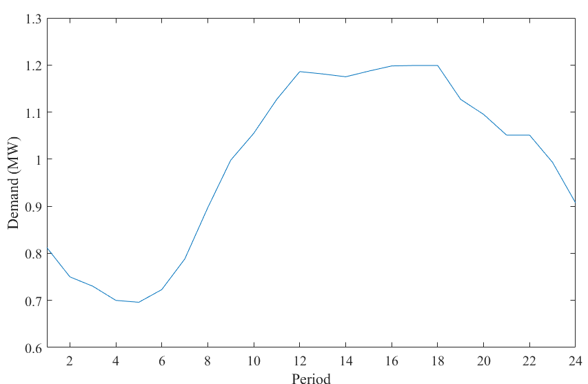
Figure 1: Energy demand in each period

The availability factor of renewable units is presented in Figure 2, this value will limit the generation of these energy sources, that is, only in period 14 (when the availability factor is equal to 1) will the sources be able to generate the equivalent of their generation capacity.

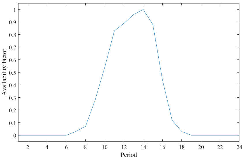
Figure 2: Availability factor of intermittent unit

III-B Results

The model proposed in Section II-A was tested on the system described in Section III-A. All simulations are performed with GAMS using a laptop with $2.4$GHz processors and $4$GB of RAM.

Three cases will be analyzed, these are:

• Case 1: Day-ahead scheduling without considering frequency reserve constraints;

• Case 2: Day-ahead scheduling with frequency reserve constraints. Only generation units participate in this service;

• Case 3: Day-ahead scheduling with frequency reserve constraints. Generation units and PEVs participate in this service;

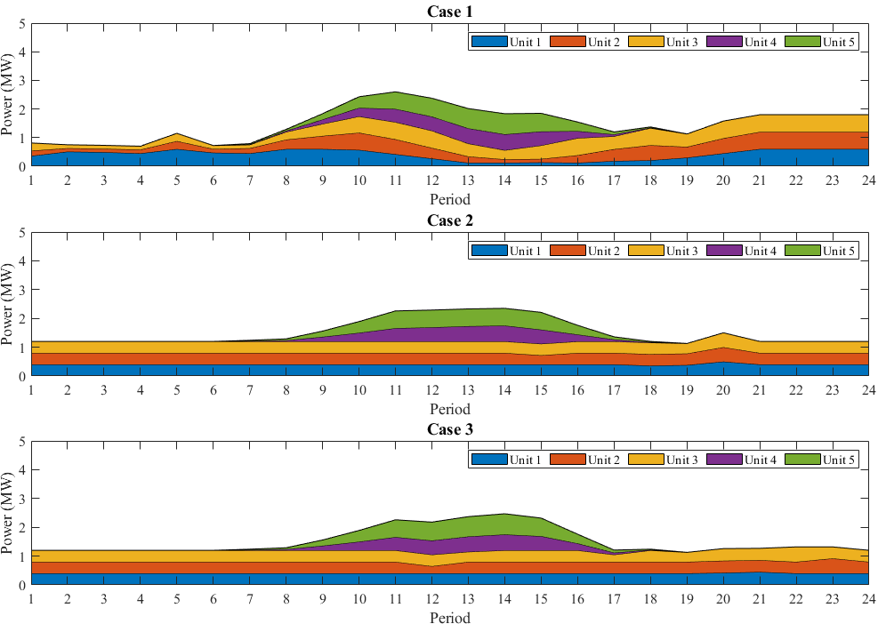
Figure 3: Power produced by units in each time period

Figure 3 shows the power produced by the generating units ($p_{gt}$) in the three considered cases. Please, observe that the first three units (Units $1$, $2$ and $3$) are conventional generating units, while the others (Units $4$ and $5$) are intermittent units. Note that when frequency regulation is not considered (Case 1), most of the energy produced in hours 1-7 is provided by Unit 1. Then, a failure of this unit may put at risk the operation of the system. However, if frequency regulation is considered, (Cases 2 and 3), the energy schedule considers the possibility of failures in the units and the demand in each hour is provided by several units. Observe that when units are operating at a low capacity level, and another unit fails, the low level unit cannot instantaneously increase to a high value of output power, due to ramp-up and ramp-down limits.

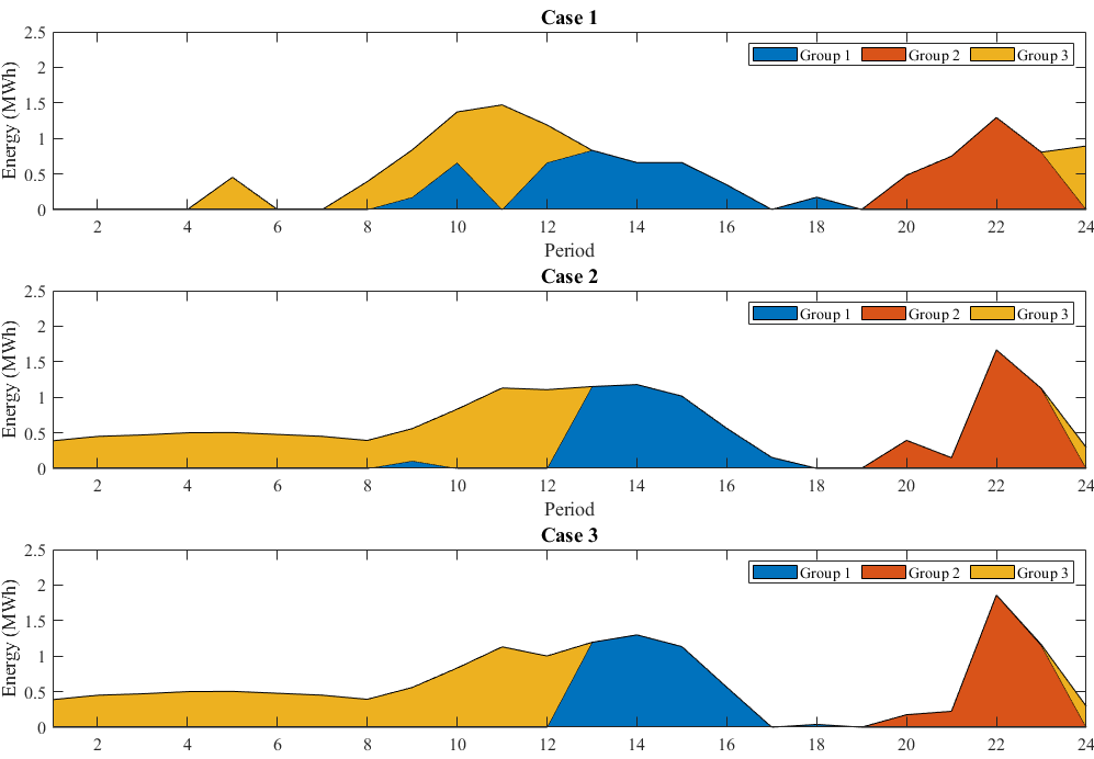
Figure 4: Energy charged by electric vehicles for each case

Figure 4 represents the energy charged ($e_{vnt}^{C}$) by electric vehicles before contingencies. It is noteworthy that when contingencies are not considered, the period in which electric vehicles are most charged is between $t=9$ and $t=16$, as it is a period with high availability of generation through renewable sources. When frequency reserve is considered, the system becomes more flexible, allowing electric vehicles to charge in other periods beyond the period in which renewable sources are available. Thus, these vehicles will provide frequency support in eventual failures of generating units.

Related to the discharged energy by PEVs, only around the instant $t=22$ do the vehicle’s discharge in all cases. Since it is a period during the night when the intermittent sources (Units $4$ and $5$) are no longer available for generation and still have relatively high demand, then PEVs can use stored energy to help meet demand.

Figure 5 shows the PFR provided by electric vehicles ($p_{vntk}^{V,PR}$). The contingency $k=1$ represents the failure of the Unit $1$, the contingency $k=2$ the Unit $2$ failure and so on.

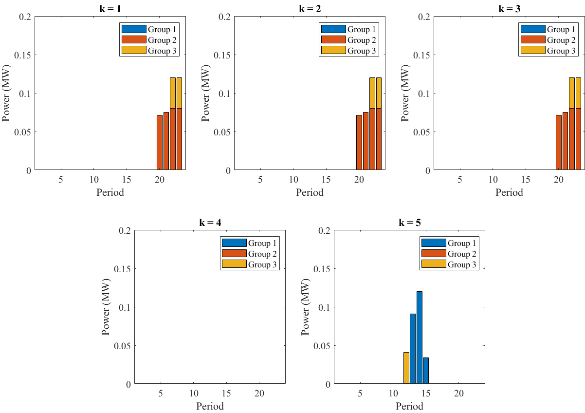
Figure 5: PFR provided by electric vehicles in case 3

It is important to note that for the first three contingencies, the vehicles provide support in frequency in the periods referring to the night period when there is no availability of intermittent sources. At $k=4$, the PEVs did not provide PFR as the generating units could provide what was needed. In the $k=5$ contingency, the vehicles provided PFR during the daytime period, as this is the contingency that represents the unit’s failure with the highest generation capacity (Unit 5). In addition, it is an intermittent unit that operates during the day.

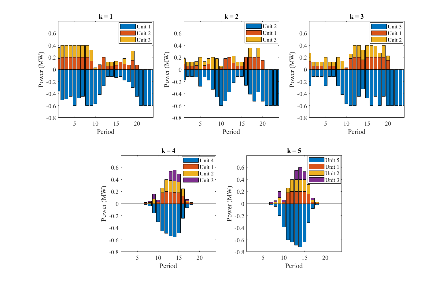
Figure 6: PFR provided by generating units in case 1

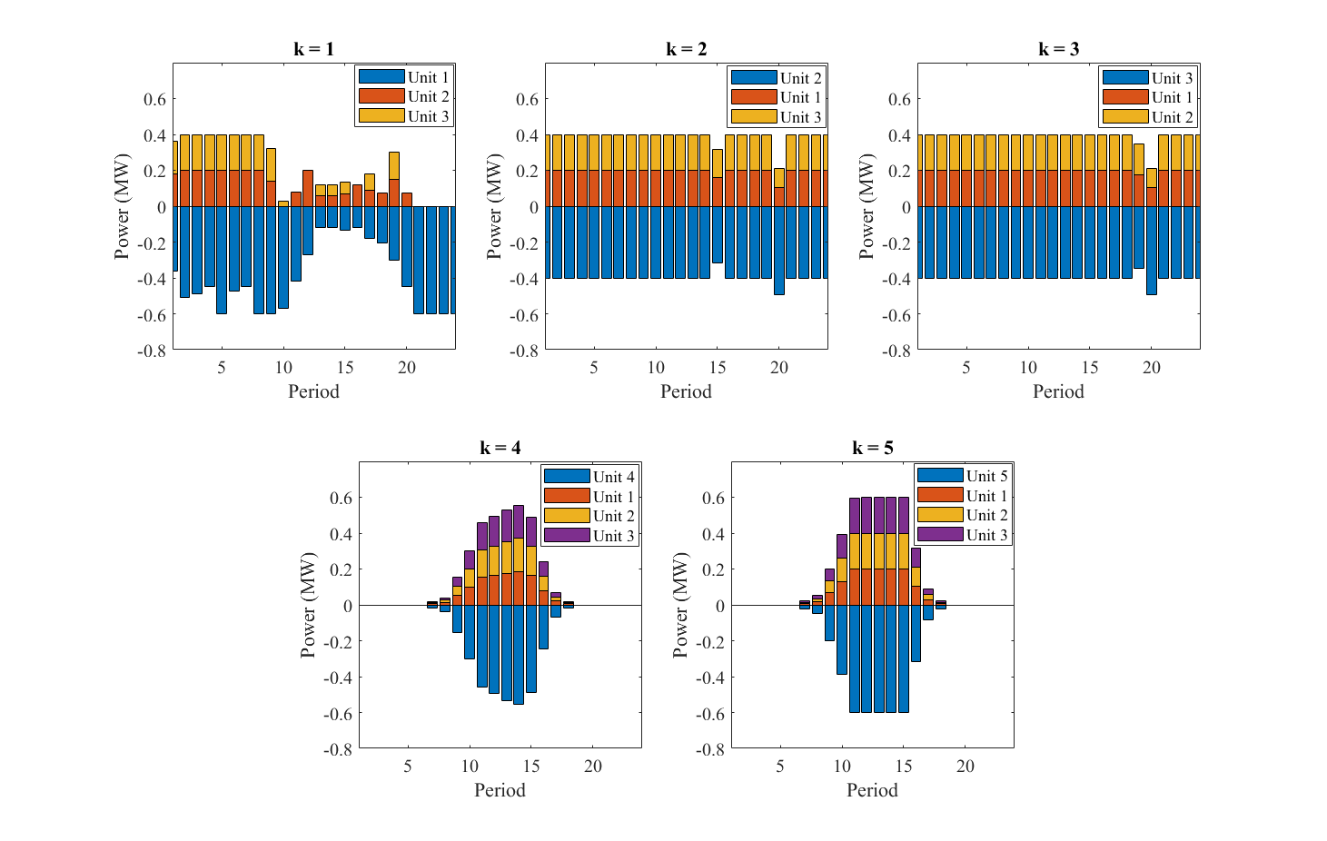
Figure 7: PFR provided by generating units in case 2

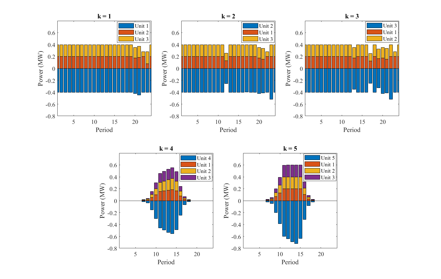
Figure 8: PFR provided by generating units in case 3

The Figures 6, 7 and 8, show the PFR provided by each generating unit ($p_{gtk}^{PR}$) in each of the 3 cases studied and after each of the contingencies. The negative values in Figures 6, 7 and 8 represent the power that the missing generator was providing before the contingency, and the positive values represent the PFR provided by the other generating units. Thus, it is ideal that there is symmetry concerning the positive and negative values, which would mean that the system can supply the power of the missing generator. Thus, note that the case with the best performance was case 3, where frequency regulation is considered, and electric vehicles participate in this service.

The frequency deviation ($\Delta f_{tk}$) is shown in Figure 9. The post-contingency states are shown on the horizontal axis, referring to each period for each contingency considered. This axis was reordered so that the frequency deviations are in ascending order, in order to obtain a better view of each case. Note that a greater frequency deviation was allowed to ensure that the unserved demand is as close to zero as possible. It is known that high-frequency variations can cause power quality problems, but as previously mentioned, a maximum frequency deviation of 1 Hz was considered. Note that Case 1 has a large number of post-contingency states with negligible frequency deviations. These post-contingency states correspond to contingencies of units with very small production.

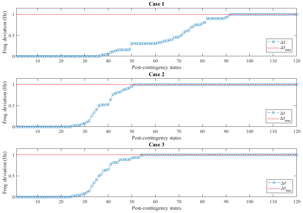
Figure 9: Frequency deviation in each period for each contingency considered for each analyzed case

Finally, post-contingency unserved demand ($p_{dtk}^{UD,PR}$) is shown in Figure 10. Note there is not unserved demand in Case 3. In Case 2, there is unserved demand only in period $t=20$ after a contingency of one of the conventional generating units ($k=1$, $k=2$ and $k=3$). Note that, in this period, the intermittent units are no longer available for generation and there is a need to charge Group 2 of electric vehicles. Finally, observe that Case 1 has a significantly higher unserved demand than the rest of cases.

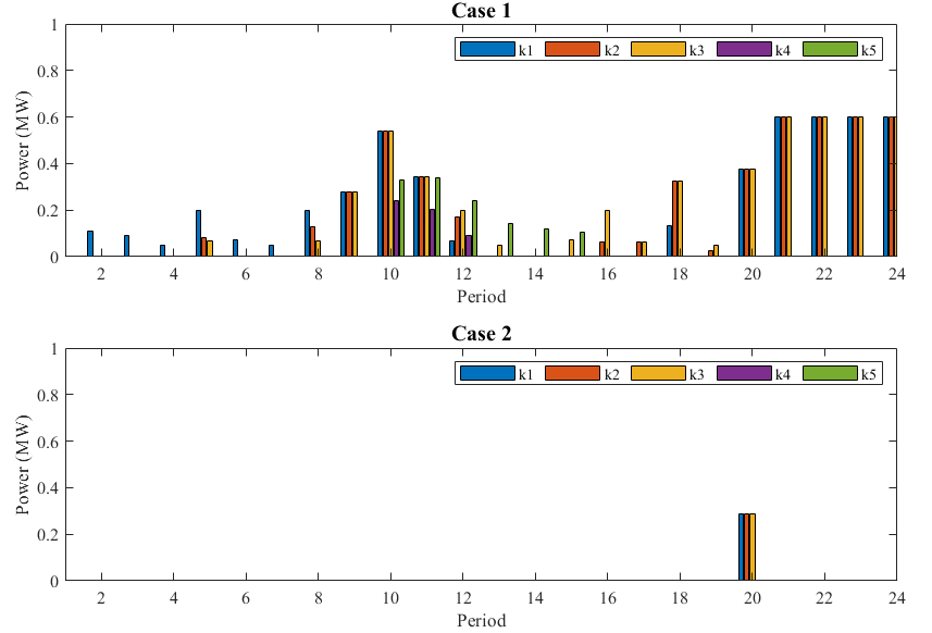
Figure 10: Unserved demand post-contingency

A presentation of the day-ahead schedule costs for each case studied is shown in Tabele IV, it is possible to observe that the largest portion of the costs in case 1 is due to unserved demand after the contingencies, and in the other cases, this value decreases considerably.

TABLE IV: Costs for each case studied (R$)

	$c_{t}^{P}$	$c_{t}^{UD,PR}$	$c_{t}^{\Delta f}$	$cc_{t}^{V}$	$cp_{t}^{V}$	Total
Case 1	14223.26	165684.05	5.41	0.00	0.00	179.91 M
Case 2	14591.18	8669.48	8.25	0.00	0.00	23.27 M
Case 3	14526.60	0.00	8.28	33.55	432.46	15.00 M

IV Conclusion

This work focused on analyzing the participation of PEVs in the day-ahead energy generating and reserve capacity scheduling, specifically, the participation of PEVs in the PFR of systems with high penetration of renewable energy sources. The proposed approach consists in a mathematical model that represents the day-ahead scheduling of a power system, which is formulated as a unit commitment problem.

The model was applied to a case study based on electrical system of the Marco Zero Campus of the Federal University of Amapá. The results obtained make it possible to verify the importance of planning the system’s operation considering the possibility of generating units failure concerning operating costs and system stability, thus making electrical power systems more flexible for the insertion of renewable sources. In addition, it was possible to estimate quantitatively the impact of the participation of PEVs in reducing the commitment of generating units that operate with a low capacity factor in the event of an unexpected generating units failure. It was possible to verify that there was a great improvement in the system operation when electric vehicles participated in different services in the system. This work also shows that in the scenario where there is a penalty for unserved demand at the Federal University of Amapá and where electric vehicles are available to provide ancillary services, the system’s operating cost reduces considerably when these PEVs participate in frequency support.

It is important to note that this work is considered a microgrid. In a large system, the contribution of electric vehicles in the system is expected to be more relevant.

References

- [1] United Nations (UN), “Paris agreement,” 2015. [Online]. Available: https://unfccc.int/sites/default/files/english_paris_agreement.pdf
- [2] ——, “The 2030 agenda for sustainable development,” 2015. [Online]. Available: https://sustainabledevelopment.un.org/content/documents/21252030%20Agenda%20for%20Sustainable%20Development%20web.pdf
- [3] International Renewable Energy Agency (IRENA). Climate change. [Online]. Available: https://www.irena.org/climatechange
- [4] Federal University of Amapá (UNIFAP). (2020) UNIFAP recebe painéis fotovoltaicos para produção de energia solar [UNIFAP receives photovoltaic panels for solar energy production]. [Online]. Available: http://www.unifap.br/unifap-recebe-paineis-fotovoltaicos-para-producao-de-energia-solar/
- [5] M. Carrión, R. Domínguez, M. Cañas-Carretón, and R. Zárate-Miñano, “Scheduling isolated power systems considering electric vehicles and primary frequency response,” Energy, vol. 168, pp. 1192–1207, 2019.
- [6] B. Dunn, H. Kamath, and J.-M. Tarascon, “Electrical energy storage for the grid: a battery of choices,” Science, vol. 334, no. 6058, pp. 928–935, 2011.
- [7] W. Kempton, V. Udo, K. Huber, K. Komara, S. Letendre, S. Baker, D. Brunner, and N. Pearre, “A test of vehicle-to-grid (v2g) for energy storage and frequency regulation in the pjm system,” Results from an Industry-University Research Partnership, vol. 32, pp. 1–32, 2008.
- [8] L. Fanglei, W. Fan, Y. Jiaming, X. Guoyi, and B. Tianshu, “Estimating maximum penetration level of renewable energy based on frequency stability constrains in power grid,” in 2020 5th Asia Conference on Power and Electrical Engineering (ACPEE), 2020, pp. 607–611.
- [9] J. Restrepo and F. Galiana, “Unit commitment with primary frequency regulation constraints,” IEEE Transactions on Power Systems, vol. 20, no. 4, pp. 1836–1842, 2005.
- [10] M. Carrión and J. M. Arroyo, “A computationally efficient mixed-integer linear formulation for the thermal unit commitment problem,” IEEE Transactions on power systems, vol. 21, no. 3, pp. 1371–1378, 2006.
- [11] M. Asensio and J. Contreras, “Stochastic unit commitment in isolated systems with renewable penetration under cvar assessment,” IEEE Transactions on Smart Grid, vol. 7, no. 3, pp. 1356–1367, 2015.
- [12] P. Mercier, R. Cherkaoui, and A. Oudalov, “Optimizing a battery energy storage system for frequency control application in an isolated power system,” IEEE Transactions on Power Systems, vol. 24, no. 3, pp. 1469–1477, 2009.
- [13] P. R. Almeida, J. P. Lopes, F. Soares, and L. Seca, “Electric vehicles participating in frequency control: Operating islanded systems with large penetration of renewable power sources,” in 2011 IEEE Trondheim PowerTech. IEEE, 2011, pp. 1–6.
- [14] Y. Yoo, S. Jung, and G. Jang, “Dynamic inertia response support by energy storage system with renewable energy integration substation,” Journal of Modern Power Systems and Clean Energy, vol. 8, no. 2, pp. 260–266, 2020.
- [15] S. Han and S. Han, “Economic feasibility of v2g frequency regulation in consideration of battery wear,” Energies, vol. 6, no. 2, pp. 748–765, 2013.
- [16] Y. Zhang, N. Rahbari-Asr, J. Duan, and M.-Y. Chow, “Day-ahead smart grid cooperative distributed energy scheduling with renewable and storage integration,” IEEE Transactions on Sustainable Energy, vol. 7, no. 4, pp. 1739–1748, 2016.
- [17] M. Aziz, “Electric vehicle utilization for ancillary grid services,” in AIP Conference Proceedings, vol. 1931, no. 1. AIP Publishing LLC, 2018, p. 030069.
- [18] S. Bellekom, R. Benders, S. Pelgröm, and H. Moll, “Electric cars and wind energy: Two problems, one solution? a study to combine wind energy and electric cars in 2020 in the netherlands,” Energy, vol. 45, no. 1, pp. 859–866, 2012.
- [19] M. Carrión and R. Zárate-Miñano, “Operation of renewable-dominated power systems with a significant penetration of plug-in electric vehicles,” Energy, vol. 90, pp. 827–835, 2015.
- [20] Plano Diretor Participativo UNIFAP. (2021) Diagnóstico energético [Energy diagnosis]. [Online]. Available: http://sites.unifap.br/planodiretor/
- [21] Agência Nacional de Energia Elétrica (ANEEL). (2021) Ranking das tarifas [Electricity tariffs ranking]. [Online]. Available: https://www.aneel.gov.br/ranking-das-tarifas