Implementation of a new weave-based search pipeline for continuous gravitational waves from known binary systems

Abstract

Scorpius X-1 (Sco X-1) has long been considered one of the most promising targets for detecting continuous gravitational waves with ground-based detectors. Observational searches for Sco X-1 have achieved substantial sensitivity improvements in recent years, to the point of starting to rule out emission at the torque-balance limit in the low-frequency range $\sim$40180\text{\,}\mathrm{H}\mathrm{z}$$. In order to further enhance the detection probability, however, there is still much ground to cover for the full range of plausible signal frequencies $\sim$201500\text{\,}\mathrm{H}\mathrm{z}$$, as well as a wider range of uncertainties in binary orbital parameters. Motivated by this challenge, we have developed BinaryWeave, a new search pipeline for continuous waves from a neutron star in a known binary system such as Sco X-1. This pipeline employs a semi-coherent StackSlide $\mathcal{F}$-statistic using efficient lattice-based metric template banks, which can cover wide ranges in frequency and unknown orbital parameters. We present a detailed timing model and extensive injection-and-recovery simulations that illustrate that the pipeline can achieve high detection sensitivities over a significant portion of the parameter space when assuming sufficiently large (but realistic) computing budgets. Our studies further underline the need for stricter constraints on the Sco X-1 orbital parameters from electromagnetic observations, in order to be able to push sensitivity below the torque-balance limit over the entire range of possible source parameters.

I Introduction

Since the first direct detection of gravitational waves from the coalescence of two stellar-mass black holes [1], we have observed more than 90 further gravitational-wave events [2, 3]. So far, all the observed signals originated from the coalescence of binary black-hole systems, binary neutron-star systems, and neutron-star-black-hole systems, each resulting in a short transient signal in the gravitational-wave detectors.

A different class of gravitational-wave signals, continuous gravitational waves (CWs) that are nearly monochromatic and long-lasting, is yet to be observed. Rapidly spinning neutron stars with some deviation from perfect axisymmetry are promising sources of such CWs in the current generation of ground-based detectors, namely Advanced-LIGO (aLIGO), Advanced-VIRGO, and KAGRA [4].

Different physical processes within a neutron star can produce CWs, resulting in different characteristics of the emitted signal. For example, a non-axisymmetric deformation (or “mountain”) on a spinning neutron star emits CWs at twice the spin-frequency, $f=2f_{\mathrm{rot}}$, while a freely precessing neutron star will additionally emit at $f\sim f_{\mathrm{rot}}$ [4]. Oscillation modes of the internal fluids in a neutron star can also produce CWs, for example, inertial r-mode oscillations emit at approximately $f\sim\frac{4}{3}f_{\mathrm{rot}}$ through the Chandrasekhar-Friedman-Schutz instability [5, 6, 4, 7].

Accreting neutron stars in galactic low-mass X-ray binary (LMXB) systems are potentially strong emitters of CWs [8, 9, 10, 11], as the accreting matter from the companion, channeled by the magnetic field of the neutron star, can result in a substantial degree of quadrupolar non-axisymmetry of the spinning neutron star [12, 13, 14].

The accreting matter also exerts a spin-up torque on the neutron star, increasing its spin frequency $f_{\mathrm{rot}}$. Interestingly, however, the observed distribution of neutron star spin frequencies shows a pronounced cut-off above $f_{\mathrm{rot}}\sim$700\text{\,}\mathrm{H}\mathrm{z}$$, well below the theoretical breakup limit of realistic neutron-star equations of state [15, 16]. Gravitational-wave emission is one of the conjectured braking mechanisms that could explain this surprising high-frequency cut-off in the spin distribution. According to the torque-balance scenario, the spin-down torque due to the emission of CWs would eventually counterbalance the accretion-induced spin-up torque. Thus, the larger the mass accretion rate, the stronger the expected gravitational-wave emission.

Sco X-1 is the brightest LMXB with one of the highest mass-accretion rates among the systems harboring a neutron star [17]. Moreover, it is relatively close to Earth, with a distance of only $\sim$ $2.8\text{\,}\mathrm{k}\mathrm{p}\mathrm{c}$ [18], making it one of the most promising sources of detectable CWs [19, 20].

Searching for CW signals in data from ground-based detectors is an active area of ongoing effort [e.g., see 4, 21, for recent overviews]. We typically classify these searches (in order of decreasing computational cost) into three main categories: all-sky searches for unknown sources over a wide range of source parameters; directed searches for sources with known sky-locations and some unknown intrinsic parameters; and targeted searches for known pulsars, where the phase evolution of the system is assumed to be known. Searches for Sco X-1 fall into the directed category, with a known sky position and unknown frequency, and substantial uncertainties on some of the binary orbital parameters.

Sco X-1 has long been considered one of the high-priority targets for CW searches, starting with [22], with further searches on initial LIGO data [23, 24, 25], and more recently on data from the Advanced LIGO detectors [26, 27, 28, 29]. Each successive search has improved constraints on the maximal strength of a putative CW signal from Sco X-1, with the latest constraints for the first time beating the above-mentioned torque-balance limit in a range of low spin frequencies $f_{\mathrm{rot}}\sim$2090\text{\,}\mathrm{H}\mathrm{z}$$ [29].

The past decade has seen the development and deployment of several pipelines for Sco X-1 searches [e.g., see 20, for an overview]. Different pipelines tend to achieve different sensitivity per computing cost and degrees of robustness against the model assumptions, such as the effect of stochastic accretion torque on the spin-frequency evolution, i.e., the so-called spin wandering [30]. Recent advances in search techniques include the adaptation of the Viterbi “hidden Markov Model” methods to searches for Sco X-1 [31, 32], and the cross-correlation CrossCorr pipeline [33, 24], which was recently improved by using resampling techniques [34] as well as efficient lattice-based template banks [35].

One of the open challenges for finding CWs from Sco X-1 stems from the fact that most of the observed neutron-star rotation rates in accreting LMXBs fall above $f_{\mathrm{rot}}\gtrsim$300\text{\,}\mathrm{H}\mathrm{z}$$ [15, 16]. Given that the mass accretion rate of Sco X-1 is one of the highest observed among all LMXBs, the neutron star would have experienced a large amount of accretion-induced spin-up torque and therefore have a high spin frequency $f_{\mathrm{rot}}$. Unfortunately, the computational cost of such a CW search grows as a substantial power of frequency $\propto f^{3-6}$, depending on the assumed parameter space [36]. Therefore, reaching or surpassing the torque-balance limit at higher spin frequencies becomes increasingly challenging.

Here we present BinaryWeave, a new directed Sco X-1 search pipeline that employs a semi-coherent $\mathcal{F}$-statistic StackSlide approach, as outlined and analyzed in Leaci and Prix [36]. This is achieved by extending the Weave framework [37], originally developed as an all-sky search for isolated neutron stars [38]. Using this framework enables us to use the fastest-available (resampling) $\mathcal{F}$-statistic algorithms and efficient lattice-based metric template banks for covering the parameter space and summing $\mathcal{F}$-statistics across segments. The tuneable segment lengths and template-bank mismatch parameters allow this pipeline to translate increases in computing budget (e.g., by using Einstein@Home [39] or a large computing cluster) into improved sensitivity [40].

BinaryWeave pipeline constructs a bank of large number of templates originating from different values of the intrinsic source parameters, e.g., spin frequency of the neutron star and orbital parameters of the binary system. Construction of a reliable and efficient template bank maximizes the detection of a weak signal above a predetermined threshold value. Often an increase in the number of templates increases the detection probability but, it also requires a higher amount of computational resources. Thus, our primary goal is to maximize the detection probability within the (varying) limitation in computing budgets. As discussed in detail in this paper (see IV and  V.3), the construction of a template bank is key to this idea.

There are two widely adopted general methodologies to construct template banks for GW searches, stochastic template banks, and geometric template banks. A geometric template bank uses algorithms to place individual templates geometrically to tile the target parameter space targeted for the search. The distance of any two adjacent templates in multi-dimensional parameter space is dictated by the maximum amount of affordable loss in signal-to-noise ratio which in turn is determined by the metric of the parameter space locally. Thus the knowledge of the parameter space metric is crucial in order to construct any geometric template bank for any search pipeline.

The main difficulty stemmed from the fact that the Sco X-1 metric changes over the parameter space [37], while the lattice-tiling Weave template-bank construction requires a strictly constant metric. We have solved this problem by developing a local approximation to the binary-orbital coordinates resulting in an “effective” constant parameter-space metric allowing for efficient lattice tiling while satisfying good coverage and mismatch properties.

We present and characterize the sensitivity and computational performance of BinaryWeave, which essentially realizes the predicted sensitivities in Leaci and Prix [36]. We discuss its applications for different astrophysical Sco X-1 scenarios, observation setups, and computing budgets. We discuss some aspects of electromagnetic observations that would help to substantially alleviate the computational challenges and improve the chances for a Sco X-1 CW detection.

This paper is organized as follows: in Sec. II we introduce the signal waveform parameters, detection statistic and template-bank construction. Section III describes the specifics of the implementation in BinaryWeave. In Sec. IV we present a detailed characterization of this new pipeline in terms of template-bank safety as well as computing-resource requirements. Section V presents the achievable sensitivities of this pipeline for different computational budgets, followed by summary and outlook in Sec. VI.

II Background

In this section we briefly introduce the concepts and notation required to understand the context of this paper (closely following [36]), namely the CW signal waveform and its parameters, the detection statistics used and the basics of metric template-bank construction.

II.1 Signal waveform and parameters

The time-dependent strain of a CW signal exerted on a gravitational-wave detector is $h(t;\mathcal{A},\lambda)$, where $t$ is the arrival time of a wavefront at the detector. The set of four amplitude parameters $\mathcal{A}$ consists of the overall amplitude $h_{0}$, the inclination angle $\cos\iota$, polarization angle $\psi$, and the initial phase $\phi_{0}$. The phase-evolution parameters $\lambda$ determine the waveform phase $\phi(t;\lambda)$ as a function of time at a given detector. The phase evolution at the detector is determined by the source-frame frequency evolution $f(\tau)$ (dependent on the intrinsic spin-evolution of the neutron star), and by the Rømer delay affecting the arrival-time $\tau(t)$ at the detector, due to the relative motion of detector and neutron star, and (if it is in a binary system) the star’s intrinsic motion around its companion star.

The neutron-star spin typically changes slowly and can therefore be represented by a Taylor-expansion around a reference time $t_{\mathrm{ref}}$, resulting in a source-frame phase model of the form

$$\phi^{\mathrm{src}}(\tau)=2\pi\left[f(\tau-t_{\mathrm{ref}})+\frac{1}{2}\dot{f}(\tau-t_{\mathrm{ref}})^{2}+\ldots\right],$$ (1)

with $f$ denoting the source-frame gravitational-wave frequency at $t_{\mathrm{ref}}$ and its higher-order derivatives, or “spindown parameters”, $f^{(k)}\equiv\left.df^{k}/d\tau^{k}\right|_{t_{\mathrm{ref}}}$.

The waveform arrival time $\tau(t)$ from the source frame $\tau$ to the detector frame $t$ is determined by the detector location and source sky-position (e.g., right ascension and declination), and by the orbital parameters describing the intrinsic neutron-star motion if it is in a binary system [41]. These consist at a minimum of the orbital projected semi-major axis $a_{\mathrm{p}}$, the period $P_{\mathrm{orb}}$ (or equivalently the mean orbital angular velocity $\Omega\equiv{2\pi}/{P_{\mathrm{orb}}}$), and a reference time of the orbit, such as the time of ascending node $t_{\mathrm{asc}}$. These parameters would fully describe the time delay in a circular orbit, while for eccentric orbits we additionally require the eccentricity $e$ and a rotation angle, such as the argument of periapsis $\omega$. For systems with small eccentricity a common reparametrization uses Laplace-Lagrange parameters $\kappa$ and $\eta$ instead, defined as

$$\kappa\equiv e\,\cos\omega,\quad\eta\equiv e\,\sin\omega.$$ (2)

In the small-eccentricity limit one can relate the time of periapsis $t_{\mathrm{p}}$ to the time of ascending node $t_{\mathrm{asc}}$ via

$$t_{\mathrm{p}}-t_{\mathrm{asc}}=\frac{\omega}{\Omega}.$$ (3)

Explicit expressions for the resulting phase model can be found in [42, 36].

II.2 Detection statistics

The gravitational-wave strain $x(t)$ observed in a detector in the presence of a signal and additive noise $n(t)$ can be written as $x(t)=n(t)+h(t;\mathcal{A},\lambda)$. The detection problem therefore corresponds to distinguishing the pure-noise hypothesis, i.e., $h(t)=0$, from the signal hypothesis with non-vanishing $h(t)$. The standard likelihood-ratio approach can be used to test different templates $h(t;\mathcal{A},\lambda)$ against the data, with a common simplification consisting in the analytic maximization over amplitude parameters, first shown in Jaranowski et al. [43], resulting in the $\mathcal{F}$-statistic. While this approach is not strictly optimal compared to Bayesian marginalization [44], it requires far less computing cost per template $\lambda$ and is therefore the current best choice for computationally-constrained wide parameter-space searches.

We denote the (coherent) statistic as $2{\mathcal{F}}(x;\lambda)$, which depends on the data $x$ and the phase-evolution parameters $\lambda$ of the waveform template for which the statistic is computed. In Gaussian noise this statistic follows a non-central $\chi^{2}$ distribution with four degrees of freedom and a non-centrality parameter ${\rho}^{2}(\mathcal{A}_{\mathrm{s}},\lambda_{\mathrm{s}};\lambda)$, where $\mathcal{A}_{\mathrm{s}}$ and $\lambda_{\mathrm{s}}$ are the (unknown) signal amplitude- and phase-evolution parameters, while $\lambda$ are the template phase-evolution parameters. The expectation value of the coherent ${\mathcal{F}}$-statistic is

$$E\left[2{\mathcal{F}}(x;\lambda)\right]=4+{\rho}^{2}(\mathcal{A}_{\mathrm{s}},\lambda_{\mathrm{s}};\lambda).$$ (4)

The noncentrality parameter ${\rho}^{2}$ characterizes the signal power in a given template, and in the coherent case its square-root ${\rho}$ is also known as the signal-to-noise ratio (SNR) for the coherent ${\mathcal{F}}$-statistic.

For wide parameter-space searches (such as for Sco X-1), some or all of the signal phase-evolution parameters $\lambda_{\mathrm{s}}$ are unknown, constrained only to fall in some astrophysically-informed parameter space $\lambda_{\mathrm{s}}\in\mathcal{P}$. The required number of templates to cover a parameter space $\mathcal{P}$ using a coherent statistic ${\mathcal{F}}$ grows rapidly as a function of the coherent integration time, which makes such searches effectively computationally impossible. Consequently, the best achievable sensitivity at a finite computational cost is typically achieved using semi-coherent statistics, as first shown in Brady et al. [45] and analyzed in more detail in [40].

The BinaryWeave pipeline as an extension of Weave [37] is based on the standard StackSlide [46] semicoherent approach using summed ${\mathcal{F}}$-statistic over shorter coherent segments. The total observation live-time $T_{\mathrm{obs}}$ is divided into $N$ shorter segments of duration $\Delta T$, i.e., in an ideal uninterrupted observation one would have $T_{\mathrm{obs}}=N\,\Delta T$. The semicoherent $\hat{\mathcal{F}}$-statistic is defined as the sum of the coherent per-segment ${\mathcal{F}}$-statistics over all $N$ segments, i.e.,

$$2\hat{\mathcal{F}}(x;\lambda)\equiv\sum^{N}_{\ell=1}2{\mathcal{F}}_{\ell}(x;\lambda).$$ (5)

This statistic follows a (non-central) $\chi^{2}$ distribution with $4N$ degrees of freedom and a noncentrality parameter (or signal power) given by

$$\hat{\rho}^{2}(x;\lambda)=\sum^{N}_{\ell=1}{\rho}^{2}_{\ell}(x;\lambda),$$ (6)

so the expectation value of $2\hat{\mathcal{F}}$ is

$$E\left[2\hat{\mathcal{F}}(x;\lambda)\right]=4N+\hat{\rho}^{2}(\mathcal{A}_{\mathrm{s}},\lambda_{\mathrm{s}};\lambda).$$ (7)

II.3 Template banks and parameter-space metrics

In order to systematically search a given parameter space $\mathcal{P}$, we need to populate it with a finite number of templates $\lambda_{\mathrm{t}}\in\mathcal{P}$. The set of all templates $\{\lambda_{\mathrm{t}}\}$ is referred to as the template bank, which is a discrete sampling of $\mathcal{P}$, i.e., $\{\lambda_{\mathrm{t}}\}\subset\mathcal{P}$. Due to this discretization of $\mathcal{P}$, a signal with parameters $\lambda_{\mathrm{s}}\in\mathcal{P}$ will not fall on an exact template, resulting in a loss of recovered signal power $\rho^{2}$ at a template $\lambda_{\mathrm{t}}$, which is quantified in terms of the mismatch $\mu_{0}$, defined as the relative loss of signal power

$$\mu_{0}(\mathcal{A}_{\mathrm{s}},\lambda_{\mathrm{s}};\lambda_{\mathrm{t}})\equiv\frac{{\rho}^{2}(\mathcal{A}_{\mathrm{s}},\lambda_{\mathrm{s}};\lambda_{\mathrm{s}})-{\rho}^{2}(\mathcal{A}_{\mathrm{s}},\lambda_{\mathrm{s}};\lambda_{\mathrm{t}})}{{\rho}^{2}(\mathcal{A}_{\mathrm{s}},\lambda_{\mathrm{s}};\lambda_{\mathrm{s}})},$$ (8)

which is a bounded function within $\mu_{0}\in[0,1]$.

Assuming a small offset $d\lambda\equiv\lambda_{\mathrm{t}}-\lambda_{\mathrm{s}}$ between signal and template and neglecting the dependence on the (unknown) signal amplitude parameters $\mathcal{A}_{\mathrm{s}}$ [47], one can define the parameter-space (phase-) metric $g_{ij}$ in terms of the truncated quadratic Taylor expansion:

$$\mu(\lambda_{\mathrm{s}};\lambda_{\mathrm{t}})=g_{ij}(\lambda_{\mathrm{s}})\,d\lambda^{i}d\lambda^{j}\,,$$ (9)

with implicit summation over the repeated indices $i,j=1,\ldots,n$, where $n$ is the number of template-bank dimensions.

The mismatch $\mu$ represents the squared distance corresponding to the parameter offsets $d\lambda$, and the metric $g_{ij}$ defines a distance measure on the parameter space. As a result, one can express the bulk number of templates $\mathcal{N}_{\mathcal{P}}$ in an $n$-dimensional lattice template bank covering the parameter space $\mathcal{P}$ with maximum mismatch $\mu_{\max{}}$ (corresponding to the squared covering radius of the lattice) [45, 48] as

$$\mathcal{N}_{\mathcal{P}}=\theta_{n}\,\mu_{\max{}}^{-n/2}\,\int_{\mathcal{P}}\sqrt{\det g(\lambda)}\,d^{n}\lambda,$$ (10)

in terms of the lattice-specific normalized thickness $\theta_{n}$; a thinner lattice will cover the same volume with fewer templates. This bulk template number ignores any extra padding typically required to fully cover the boundary $\partial\mathcal{P}$ of the parameter space $\mathcal{P}$, which tends to increase the total number of templates in practice [e.g., see 49, 37].

The metric allows for a simple estimate of the approximate scale of the template-bank resolution along single coordinates via

$$\delta\lambda^{i}=2\sqrt{\frac{\mu_{\max{}}}{g_{ii}}}\,,$$ (11)

which is obtained from Eq. (9) by assuming a single nonzero offset along one coordinate axis $\delta\lambda^{i}$. In a one-dimensional template-bank grid, the factor of two accounts for the fact that the maximum mismatch $\mu_{\max{}}$ would be attained at the mid-point between two lattice templates. The true higher-dimensional grid spacings will typically be larger than this estimate, however, due to potential nonzero cross-terms $g_{ij}$ that come into play when considering generic offsets, as well as using other lattice structures than a simple rectangular grid along coordinate axes.

A somewhat complementary grid-scale estimate can be obtained from considering the extents of the bounding box [36] around a metric ellipse of constant mismatch Eq. (9), namely

$$D\lambda^{i}=2\sqrt{\mu_{\max{}}\,(g^{-1})^{ii}}\,,$$ (12)

where $g^{-1}$ is the inverse matrix of the metric $g$. Contrary to Eq. (11), this fully takes into account parameter correlations, but will generally result in an overestimate of the actual lattice grid spacing [50, 47].

The coherent phase metric ${g}_{ij}(\lambda)$ at a parameter-space point $\lambda$ (ignoring the (unknown) signal amplitude parameters $\mathcal{A}_{\mathrm{s}}$) can be shown [45, 47] to be expressible directly in terms of derivatives of the signal phase $\phi(t;\lambda)$, namely

$${g}_{ij}(\lambda)=\left\langle{\partial_{i}\phi(\lambda)\,\partial_{j}\phi(\lambda)}\right\rangle-\left\langle{\partial_{i}\phi(\lambda)}\right\rangle\,\left\langle{\partial_{j}\phi(\lambda)}\right\rangle\,,$$ (13)

where $\partial_{i}\phi(\lambda)\equiv\partial\phi/\partial\lambda^{i}$ and $\left\langle{Q}\right\rangle$ denotes time averaging of a quantity $Q$ over the coherent duration $\Delta T$, i.e., $\left\langle{Q}\right\rangle\equiv({1}/{\Delta T})\int_{t0}^{t0+\Delta T}Q(t)\,dt$.

The corresponding semicoherent metric $\hat{g}_{ij}(\lambda)$ at a point $\lambda$ can then be obtained [51] as the average over segments, namely

$$\hat{g}_{ij}(\lambda)=\frac{1}{N}\sum_{\ell=1}^{N}{g}_{\ell,ij}(\lambda),$$ (14)

where ${g}_{\ell,ij}$ is the coherent metric of segment $\ell$.

II.4 Sco X-1 parameter-space metric

A number of rapidly spinning neutron stars in LMXB systems are found to be in (approximate) spin equilibrium [52, 53, 54]. According to the gravitational-wave torque-balance hypothesis, the total amount of accretion-induced spin-up torque would be counter-balanced by the braking torques due to the emission of CWs and electromagnetic radiation [9]. This keeps the system in approximate torque balance, with random fluctuations in spin frequency due the stochastic nature of the accretion flows, which is known as spin wandering [55, 30].

Similar to previous studies, and following [36], we therefore assume a constant intrinsic signal frequency $f$ with no long-term drifts, i.e., $f^{(k\geq 1)}=0$, and we tackle the spin-wandering effect by limiting the maximal segment length $\Delta T$ such that the frequency resolution is still too coarse for any spin wandering effect to move the signal by more than one frequency bin.

We can therefore use the following physical phase-evolution parameters describing the CW waveforms

$$\lambda=\{f,a_{\mathrm{p}},t_{\mathrm{asc}},\Omega,\kappa,\eta\},$$ (15)

and assuming the small-eccentricity limit for Sco X-1, i.e., $e\ll 1$, the approximate CW phase model [42, 36] can be written as

$$\frac{\phi(t;\lambda)}{2\pi}\approx f\Delta t-fa_{\mathrm{p}}\left[\sin\Psi+\frac{\kappa}{2}\sin 2\Psi-\frac{\eta}{2}\cos 2\Psi\right],$$ (16)

where $\Delta t\equiv t-t_{\mathrm{ref}}$ and the orbital phase $\Psi(t)$ is given by

$$\Psi(t)=\Omega\,(t-t_{\mathrm{asc}}).$$ (17)

From the explicit expression Eq. (16) of the phase one can obtain the phase derivatives $\partial_{i}\phi$ with respect to the parameter-space coordinates $\lambda^{i}$, and time-averaging yields the coherent metric components ${g}_{\ell,ij}$ for each segment $\ell$ according to Eq. 13. The semi-coherent metric $\hat{g}_{ij}$ is then obtained by averaging over segments following Eq. 14.

In the template-bank construction the metric will typically be computed numerically starting from the analytic expressions for the phase derivatives. However, it is important to also consider approximate analytic expressions for these metrics, in order to better understand their properties. As discussed in [42, 36], analytic approximations can be found in the two limiting cases: short segments where $\Delta T\ll P_{\mathrm{orb}}$, or long segments where $\Delta T\gg P_{\mathrm{orb}}$. Longer segments will result in better sensitivity but also higher computational cost. The results in [36] indicate that using a realistically large computational budget, semi-coherent $\hat{\mathcal{F}}$-statistic searches for Sco X-1 can afford segments substantially longer than $P_{\mathrm{orb}}\sim$19\text{\,}\mathrm{h}$$. Therefore we will only discuss the long-segment limit here, for which the nonzero elements in the analytic approximation to the semi-coherent metric are found [36] as

$$\hat{g}_{ff} =\pi^{2}\frac{\Delta T^{2}}{3}\,,$$ (18)

$$\hat{g}_{a_{\mathrm{p}}a_{\mathrm{p}}} =2\pi^{2}f^{2}\,,$$

$$\hat{g}_{\Omega\Omega} =2\pi^{2}(fa_{\mathrm{p}})^{2}\left(\frac{\Delta T^{2}}{12}+\overline{\Delta_{\mathrm{ma}}^{2}}\right)\,,$$

$$\hat{g}_{t_{\mathrm{asc}}t_{\mathrm{asc}}} =2\pi^{2}(fa_{\mathrm{p}}\Omega)^{2}\,,$$

$$\hat{g}_{\Omega t_{\mathrm{asc}}} =\hat{g}_{t_{\mathrm{asc}}\Omega}=-2\pi^{2}(fa_{\mathrm{p}})^{2}\,\Omega\,\overline{\Delta_{\mathrm{ma}}}\,,$$

$$\hat{g}_{\kappa\kappa} =\hat{g}_{\eta\eta}=\frac{\pi^{2}}{2}(fa_{\mathrm{p}})^{2}\,,$$

where $\Delta_{\mathrm{ma},\ell}\equiv t_{\mathrm{mid},\ell}-t_{\mathrm{asc}}$ is the time offset between the midpoint $t_{\mathrm{mid},\ell}$ of segment $\ell$ and the ascending node $t_{\mathrm{asc}}$, and where $\overline{Q}$ denotes averaging over segments, i.e., $\overline{Q}\equiv(1/N)\sum^{N}_{\ell=1}Q_{\ell}$. Note that the coherent per-segment metric ${g}_{\ell,ij}$ can simply be read-off these expressions as the special case $\ell=N=1$.

There are two important aspects to consider about this metric:

1. The metric components still depend on the search parameters $f,a_{\mathrm{p}},\Omega$ and $t_{\mathrm{asc}}$ and are therefore not constant over the parameter space. This is an obstacle to constructing a lattice template-bank, which will be dealt with in Sec. III.

2. There is little refinement of the semi-coherent metric compared to the per-segment coherent resolution, in fact most components do not depend on the number of segments (i.e., the total duration of data used for the searches) for a fixed duration of coherent segment $\Delta T$, except for $\hat{g}_{\Omega\Omega}$ (via $\overline{\Delta_{\mathrm{ma}}^{2}}$) and $\hat{g}_{\Omega t_{\mathrm{asc}}}$ (via $\overline{\Delta_{\mathrm{ma}}}$).

In order to simplify the expression, we can make use of the gauge freedom in $t_{\mathrm{asc}}$, which is only defined up to an integer multiple of the period $P_{\mathrm{orb}}$, i.e.,

$$t_{\mathrm{asc}}^{\prime}=t_{\mathrm{asc}}+n\,P_{\mathrm{orb}},\quad\text{for}\quad n\in\mathbb{Z},$$ (19)

describes the same physical orbit, as seen in Eqs. (16),(17). Given the long-segment assumption $\Delta T\gg P_{\mathrm{orb}}$, the total observation time will satisfy this even more strongly, i.e., $T_{\mathrm{obs}}\geq N\,\Delta T\gg P_{\mathrm{orb}}$. One can therefore chose a gauge $t_{\mathrm{asc}}\approx\overline{t_{\mathrm{mid}}}$ such that $\overline{\Delta_{\mathrm{ma}}}\approx 0$, removing the only nonzero off-diagonal component $g_{\Omega t_{\mathrm{asc}}}$. Further, assuming gapless segments one can show [36] that in this case

$$\hat{g}_{\Omega\Omega}=\frac{\pi^{2}}{6}(fa_{\mathrm{p}})^{2}\,(N\,\Delta T)^{2},$$ (20)

in other words, only the semi-coherent resolution in $\Omega$ increases with the number of segments, while all other parameters have the same metric resolution per segment and in the semi-coherent combination. This point will be further discussed in Sec. III on the details of the BinaryWeave implementation.

II.5 Lattice-tiling template banks

The template-bank construction in BinaryWeave is directly inherited from Weave, described in full detail in [49, 37], therefore we only provide a short overview here. The basic inputs to the lattice-tiling algorithm are the parameter-space coordinates $\{\lambda^{i}\}$, boundaries defining $\mathcal{P}$, and the corresponding template-bank metric, which must be constant over the search space. The code can use a coordinate-transformation to internal coordinates if the metric is expressed in different coordinates than the standard CW waveform parameters described in Sec. II.1. Based on these inputs, together with a maximum-mismatch parameter $\mu_{\max{}}$ and a choice of lattice type, the algorithm constructs a template-bank lattice with covering radius $\sqrt{\mu_{\max{}}}$ tiling the parameter space (and ensuring appropriate covering of the boundaries).

There are two main modes semi-coherent statistics can be computed over the set of segments: interpolating and non-interpolating. As mentioned in Sec. II.4, the semi-coherent template bank requires a finer resolution in $\Omega$ to compute $\hat{\mathcal{F}}$ than the per-segment template banks to compute ${\mathcal{F}}_{\ell}$ at given maximum-mismatch $\mu_{\max{}}$. This can be used to save computing power, by using coarser per-segment template banks together with a nearest-neighbor interpolation when picking per-segment ${\mathcal{F}}_{\ell}$ to sum in Eq. (5). The details and effects of such an interpolating StackSlide approach are discussed in [40]. The simpler, yet generally more computationally expensive, method consist in using the same semi-coherent fine grid over all segments, such that Eq. (5) can directly be computed without any interpolation.

The amount of computing-cost savings due to interpolation depends on the refinement factor between coherent and semi-coherent metrics, which in the case of the Sco X-1 metric is only linear in $N$ if including $\Omega$ in the template bank, and unity otherwise, as discussed in Sec. II.4. The expected sensitivity gains by using interpolation in this case would therefore be modest and partially reduced by the extra mismatch incurred due to interpolation itself [see 40]. Furthermore, it is more difficult to find optimal setup parameters for an interpolating setup, given there are two mismatch parameters $\{{\mu}_{\max{}},\hat{\mu}_{\max{}}\}$ to tune rather than a single $\mu_{\max{}}$, in addition to the number $N$ and length $\Delta T$ of the semi-coherent segments.

The $A_{n}^{*}$ lattice is a common choice [56, 49, 37, 57] as a close-to-optimal template-bank lattice to use, based on earlier arguments about optimal covering lattices [48, 58]. Recent work [59, 60] has clarified, however, that finding the template-bank lattice that maximizes the expected detection probability at fixed number of templates is an instance of the quantizer problem [58], not the covering problem. This changes somewhat the choice of current “record holder” lattice in each dimension, and reduces the relative advantage of $A_{n}^{*}$ over the hyper-cubic lattice, but even in this paradigm $A_{n}^{*}$ remains a close-to-optimal lattice and therefore continues to be a practically reasonable and sound choice.

II.6 Sco X-1 parameter space

Optical and X-ray observations tell us that Sco X-1 is an LMXB system [61]. Furthermore, X-ray spectral and timing characteristics indicate that the compact object in the Sco X-1 binary system is a neutron star [17]. Observations in optical and radio bands have constrained the three orbital parameters $a_{\mathrm{p}}$, $P_{\mathrm{orb}}$, and $t_{\mathrm{asc}}$ of Sco X-1 to different extents [18, 62, 63], namely $a_{\mathrm{p}}\in[1.45,3.25]\,$\mathrm{l}\mathrm{s}$$, $P_{\mathrm{orb}}\sim$68\,023.86048\pm 0.0432\text{\,}\mathrm{s}$$ and $t_{\mathrm{asc}}\sim$974\,416\,624\pm 50\text{\,}\mathrm{G}\mathrm{P}\mathrm{S}\,\mathrm{s}$$ (as used in a recent CW search [28]. while the spin frequency of the neutron star still remains practically unconstrained [64, 65] to date. We provide a table of various Sco X-1 parameter-space ranges considered in this and past studies (and searches) in Table. 1, which will be discussed in more detail in Sec. V.2.

The typical life-cycle of an LMXB along with one of the highest mass-accretion rate systems indicate that the neutron star in Sco X-1 is likely to receive a large amount of accretion-induced spin-up torque [55] and is plausibly spinning rapidly. Most of the accreting neutron stars in LMXB systems are observed to be spinning in the range of $\sim$300600\text{\,}\mathrm{H}\mathrm{z}$$, although a few of them have also been observed at lower spin frequencies [66, 15]. We explore the implications of different assumptions about the spin and orbital parameters of Sco X-1 for a wide-parameter search in subsection V.2.

III Flat metric approximation

As discussed in Sec. II.4, the long-segment binary parameter-space metric Eq. (18) in physical coordinates is not constant over $\{f,a_{\mathrm{p}},\Omega,t_{\mathrm{asc}}\}$, which prohibits its direct use for lattice tiling. This represents the main obstacle to applying the Weave framework to a directed binary search.

Regarding the frequency dependence, all metric components (except $g_{ff}$) scale as $f^{2}$, as the signal phase at the detector is $\phi(t)\sim 2\pi f\,\tau(t)$ and the metric (13) is quadratic in phase. This scaling is similar to the metric over the sky position parameters, and may be mitigated in the same way [e.g. 67]: a full search is typically broken into smaller workunits distributed over nodes of a cluster (or Einstein@Home), where each workunit would analyze a relatively narrow frequency band $\lesssim\mathcal{O}\left($1\text{\,}\mathrm{H}\mathrm{z}$\right)$. We can therefore deal with the frequency dependence by simply evaluating the metric at a fixed frequency within each narrow range, typically at the highest frequency to guarantee the given maximum-mismatch constraint over the search band, accepting small relative changes of the mismatch distribution over the frequency band.

A similar argument applies to $t_{\mathrm{asc}}$ in the long-segment regime: due to the gauge freedom Eq. (19), the maximal physical uncertainty for any system would be $\Delta t_{\mathrm{asc}}<P_{\mathrm{orb}}\ll\Delta T$, and can therefore be neglected in $g_{\Omega\Omega}$, as seen in Eq. (20), which is the only metric term that would be affected by this.

Given the narrow astrophysical uncertainties on $P_{\mathrm{orb}}$ for Sco X-1 (cf. Sec. II.6), this approach could also be used for $\Omega$, but it would be very specific to Sco X-1 and might not apply to other directed binary searches. Furthermore, ignoring the metric changes over the astrophysical range on $a_{\mathrm{p}}$ would not work well for Sco X-1, given the currently uncertainty spans more than a factor of two.

We observe that the metric Eq. (18) depends on $a_{\mathrm{p}}$ and $\Omega$ only via quadratic scaling of some components, i.e., the metric stretches or contracts along certain directions in parameter space. In order to absorb this scaling, we only need to assume that the metric change is negligible on the scale $\delta\lambda$ of a lattice cell, so we can resort to local rescaling via the following “pseudo” coordinate transformation of $\{\Omega,t_{\mathrm{asc}},\kappa,\eta\}$ into:

$$v_{\mathrm{p}} \equiv\underline{a_{\mathrm{p}}}\,\Omega,$$ (21)

$$d_{\mathrm{asc}} \equiv\underline{a_{\mathrm{p}}}\,\underline{\Omega}\,t_{\mathrm{asc}},$$

$$\kappa_{\mathrm{p}} \equiv\underline{a_{\mathrm{p}}}\,\kappa,$$

$$\eta_{\mathrm{p}} \equiv\underline{a_{\mathrm{p}}}\,\eta,$$

where $\underline{a_{\mathrm{p}}}$ and $\underline{\Omega}$ will be treated as constant scaling parameters in derivatives. Substituting the new coordinates in Eq. (16) results in the (orbital) phase model

$$\frac{\phi_{\mathrm{orb}}(t;\lambda)}{2\pi} =-fa_{\mathrm{p}}\left(\sin\Psi+\frac{\kappa_{\mathrm{p}}}{2\underline{a_{\mathrm{p}}}}\sin 2\Psi-\frac{\eta_{\mathrm{p}}}{2\underline{a_{\mathrm{p}}}}\cos 2\Psi\right),$$ (22)

$$\Psi(t) =\frac{v_{\mathrm{p}}}{\underline{a_{\mathrm{p}}}}\left(t-\frac{d_{\mathrm{asc}}}{\underline{a_{\mathrm{p}}}\,\underline{\Omega}}\right),$$

and the following approximate phase derivatives:

$$\partial_{v_{\mathrm{p}}}\phi =-2\pi f(t-t_{\mathrm{asc}})\,[\cos\Psi+\kappa\cos 2\Psi+\eta\sin 2\Psi]\,,$$ (23)

$$\partial_{d_{\mathrm{asc}}}\phi =2\pi f\,[\cos\Psi+\kappa\cos 2\Psi+\eta\sin 2\Psi]\,,$$

$$\partial_{\kappa_{\mathrm{p}}}\phi =-\pi f\sin 2\Psi\,,$$

$$\partial_{\eta_{\mathrm{p}}}\phi =\pi f\cos 2\Psi.$$

Applying the steps of Sec. II.3 this yields the following metric components (with $\hat{g}_{ff}$ and $\hat{g}_{a_{\mathrm{p}}a_{\mathrm{p}}}$ unchanged from Eq. (18)):

$$\hat{g}_{v_{\mathrm{p}}v_{\mathrm{p}}} =2\pi^{2}f^{2}\,\left(\frac{\Delta T^{2}}{12}+\overline{\Delta_{\mathrm{ma}}^{2}}\right)\,,$$ (24)

$$\hat{g}_{d_{\mathrm{asc}}d_{\mathrm{asc}}} =2\pi^{2}f^{2}\,,$$

$$\hat{g}_{v_{\mathrm{p}}d_{\mathrm{asc}}} =\hat{g}_{d_{\mathrm{asc}}v_{\mathrm{p}}}=-2\pi^{2}f^{2}\,\overline{\Delta_{\mathrm{ma}}}\,,$$

$$\hat{g}_{\kappa_{\mathrm{p}}\kappa_{\mathrm{p}}} =\hat{g}_{\eta_{\mathrm{p}}\eta_{\mathrm{p}}}=\frac{\pi^{2}}{2}f^{2}\,,$$

which are constant over $a_{\mathrm{p}}$ and $\Omega$ and are therefore suitable for lattice tiling within the Weave framework.

We are applying the coordinate transformation Eq. (21) globally over the search parameter space, but ignore the local changes in $a_{\mathrm{p}},\Omega$-scaling within each lattice cell. This should be a good approximation as long as cells are small compared to the effects of changing $a_{\mathrm{p}},\Omega$ over their respective length scales.

We have thoroughly tested the safety and effectiveness of this metric approximation for a Sco X-1 search, which is discussed in the next section.

IV Testing and characterization

The semi-coherent $\hat{\mathcal{F}}$-statistic in BinaryWeave is computed by the well-tested Weave framework [37] using the standard LALSuite [68] $\mathcal{F}$-statistic implementation. The behavior of this statistic implementation in recovering signals in noise is therefore already well understood and tested. Therefore, the only new elements requiring careful testing and characterization are the template-bank mismatch and the computing cost. For this reason, we have limited the mismatch characterization studies for the signal-only cases without introducing any kind of GW detector noises.

IV.1 Test setup and assumptions

The metric and template bank implemented in BinaryWeave can in principle handle eccentricity within the small-eccentricity approximation $e\ll 1$ of Eq. (16), which in [36] was seen to hold up to about $e\lesssim 0.1$. The orbital eccentricity of Sco X-1 is currently poorly constrained, but expected to be close to zero due to Roche-lobe overflow accretion [63]. In order to simplify this first proof-of-concept study of BinaryWeave, we are assuming negligible eccentricity here and focus on purely circular orbits. Therefore we consider a Sco X-1 search parameter space $\mathcal{P}$ that is (at most) four-dimensional (4D), with search parameters $\{f,a_{\mathrm{p}},P_{\mathrm{orb}},t_{\mathrm{asc}}\}$.

The orbital period $P_{\mathrm{orb}}$ for Sco X-1 is constrained to about $\Delta P_{\mathrm{orb}}\sim$0.04\text{\,}\mathrm{s}$$, compared to a period of $P_{\mathrm{orb}}\sim$19\text{\,}\mathrm{h}$$ (cf. Sec. II.6). The search resolution $\delta\Omega$ (and therefore also $\delta P_{\mathrm{orb}}$) in Eq. (11) is determined by the metric (in particular $\hat{g}_{\Omega\Omega}$ of Eq. (20)) and therefore depends on the search setup $\{N,\Delta T,\mu_{\max{}}\}$, the search frequency $f$, and semi-major axis $a_{\mathrm{p}}$. In particular, the resolution increases linearly with total search duration $T_{\mathrm{obs}}=N\,\Delta T$, and for longer-duration searches (e.g., $T_{\mathrm{obs}}\sim$6\text{\,}\mathrm{m}\mathrm{o}\mathrm{n}\mathrm{t}\mathrm{h}\mathrm{s}$$) will often fully resolve the parameter-space uncertainty in period, i.e., $\delta P_{\mathrm{orb}}<\Delta P_{\mathrm{orb}}$. However, for coarser search setups, or assuming future improved observational constraints, it can also be sufficient to place a single template at the mid-point of the uncertainty range, resulting in a three-dimensional (3D) search space $\mathcal{P}$ spanning only $\{f,a_{\mathrm{p}},t_{\mathrm{asc}}\}$. In the following we will therefore consider both possibilities of 3D and 4D template banks.

In this study we are exclusively using the non-interpolating StackSlide Weave mode, which is simpler and easier to optimize for, while expected to yield similar sensitivity for directed binary searches, as discussed in Sec. II.5. This means that the coherent segments and final semi-coherent statistic use the same template grid and there is only a single mismatch parameter $\hat{\mu}_{\max{}}={\mu}_{\max{}}$.

All subsequent simulations use $\mathcal{F}$-statistic input data split into short Fourier-transforms (SFT) [69] of baseline $T_{\mathrm{sft}}\leq$250\text{\,}\mathrm{s}$$, which is a safe SFT length over the Sco X-1 parameter space, e.g., see Eq.(C2) in [36]. Furthermore, all simulations assume data from two detectors, namely LIGO Hanford (H1) and LIGO Livingston (L1).

IV.2 Template-bank mismatch

In order to ensure the validity of the constructed lattice template banks using the approximately-flat metric constructed in Sec. III, we perform injection-recovery Monte-Carlo tests. These tests are typically performed without noise, i.e., searching a data stream only containing the injected signal waveform. This allows one to directly measure signal power without noise bias and to accurately calculate the mismatch, which is the main purpose of template bank tests. The signal parameters for the injections are drawn uniformly from the (wider) testing Sco X-1 parameter-space $\mathcal{P}_{0}$ specified in Table. 1, with randomly drawn amplitude parameters $\mathcal{A}$, and a search grid is constructed around the injection point (randomly shifted to avoid systematic alignment effects).

A good template bank should satisfy the maximal mismatch criterion [e.g. 48]: the measured mismatch $\mu_{0}(\lambda_{\mathrm{s}};\lambda_{\mathrm{t}})$ of Eq. (8) for any injected signal $\lambda_{\mathrm{s}}\in\mathcal{P}$ at its “closest” (i.e., highest signal power $\rho^{2}$) template $\lambda_{\mathrm{t}}$ should be less than the maximum mismatch $\mu_{\max{}}$ the template bank was constructed for, which can formally be written as

$$\max_{\lambda_{\mathrm{s}}\in\mathcal{P}}\min_{\lambda_{\mathrm{t}}}\,\mu_{0}(\lambda_{\mathrm{s}};\lambda_{\mathrm{t}})\leq\mu_{\max{}},$$ (25)

where the “minimax” formulation (constraining the nearest-template mismatch at the worst-case signal location) implies that the mismatch is constrained for all possible signal locations.

Furthermore, an efficient template bank should ideally place only a single template within $\mu_{\max{}}$ of any signal, to avoid (computationally wasteful) over-resolution and producing excessive candidates per signal that would require some form of clustering or follow-up (see also [38]).

We have performed a number of signal injection-recovery tests of the BinaryWeave template banks for various different search setups $\{N,\Delta T,\mu_{\max{}}\}$. Here we only present a few representative examples in order to illustrate the main features of these template banks: in Sec. IV.2.1 we illustrate the template grids for single-parameter (1D) and two-parameters (2D) searches, and in Sec. IV.2.2 we provide examples of the mismatch distribution for 3D searches (for a non-resolved period uncertainty $\Delta P_{\mathrm{orb}}$) and full 4D searches.

IV.2.1 Testing 1D and 2D lattice tilings

(a)                                                                  (b)

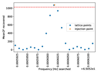
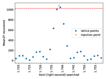
(c)                                                                  (d)

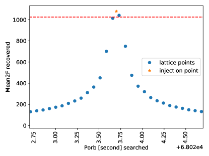
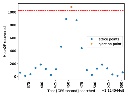
Figure 1: Illustration of 1D template-bank searches around a noiseless signal injection, with the respective three remaining search parameters fixed to the injected signal. The filled circles mark the placement of templates and their corresponding measured $\hat{\mathcal{F}}$-statistic values, while the star marks the signal injection point with its corresponding perfect-match $\hat{\mathcal{F}}$-statistic. The template bank was constructed for a maximum mismatch of $\mu_{\max{}}=0.05$, with $N=120$ segments of $\Delta T=$3\text{\,}\mathrm{d}$$. The horizontal dashed line denotes the $\hat{\mathcal{F}}$-value corresponding to the maximum-mismatch criterion Eq. (25) relative to the injected signal power.

In order to illustrate and visualize the lattice tiling, we first consider simple one- and two-dimensional lattice cases, which also serve as a basic sanity check for the template bank construction. The 1D searches are performed along all four coordinate axis in a neighborhood around the signal injection, with the three remaining parameters fixed to the injection values, with one example shown in Fig. 1.

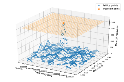
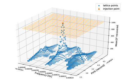
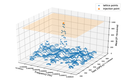
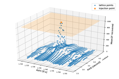
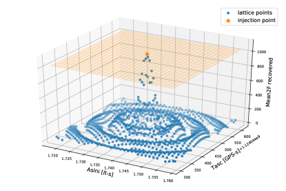
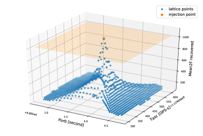
Figure 2: Illustration of 2D template-bank searches around a noiseless signal injection, with the respective two remaining search parameters fixed to the injected signal. The filled circles mark the placement of templates and their corresponding measured $\hat{\mathcal{F}}$-statistic values, while the star marks the signal injection point with its corresponding perfect-match $\hat{\mathcal{F}}$-statistic. The template bank was constructed for a maximum mismatch of $\mu_{\max{}}=0.05$, with $N=120$ segments of $\Delta T=$3\text{\,}\mathrm{d}$$. The horizontal mesh grid denotes the $\hat{\mathcal{F}}$-value corresponding to the maximum-mismatch criterion Eq. (25) relative to the injected signal power.

The 2D searches are performed along all six two-parameter combinations out of the four, with the remaining two parameters fixed to the injected signal location, with one example shown in Fig. 2.

These results illustrate the maximum-mismatch criterion of Eq. 25 being satisfied, as well as placing only one template in the “vicinity” $<\mu_{\max{}}$ of the signal as desired for an efficient template bank.

IV.2.2 Testing 3D and 4D lattice tilings

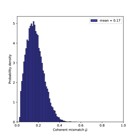
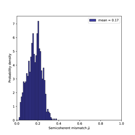
Figure 3: Distribution of coherent per-segment mismatches ${\mu}_{0}$ (left plot) and semi-coherent mismatches $\hat{\mu}_{0}$ (right plot), obtained from $1000$ simulated 3D searches over a small box in $f$, $a_{\mathrm{p}}$ and $t_{\mathrm{asc}}$ around the injected signals (with $P_{\mathrm{orb}}$ fixed at its injection value), with parameters drawn randomly from the test range $\mathcal{P}_{0}$ defined in Table. 1. The template bank was constructed for a maximum mismatch of $\mu_{\max{}}=0.5$, with $N=30$ segments of $\Delta T=$1\text{\,}\mathrm{d}$$.

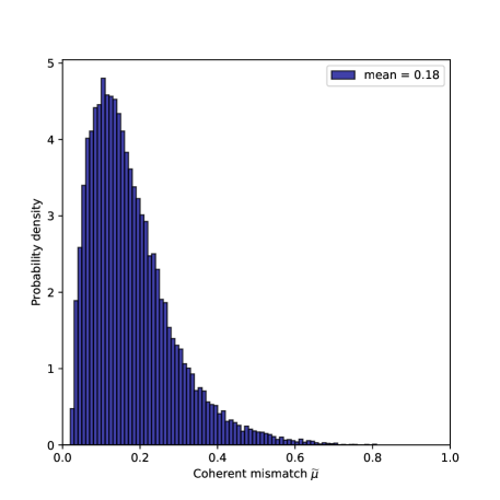
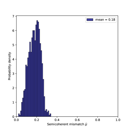
Figure 4: Distribution of coherent per-segment mismatches ${\mu}_{0}$ (left plot) and semi-coherent mismatches $\hat{\mu}_{0}$ (right plot), obtained from $1000$ simulated 4D searches over a small box in $f,a_{\mathrm{p}},t_{\mathrm{asc}}$ and $P_{\mathrm{orb}}$ around the injected signals, with parameters drawn randomly from the test range $\mathcal{P}_{0}$ defined in Table. 1. The template bank was constructed for a maximum mismatch of $\mu_{\max{}}=0.5$, with $N=30$ segments of $\Delta T=$1\text{\,}\mathrm{d}$$.

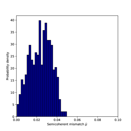
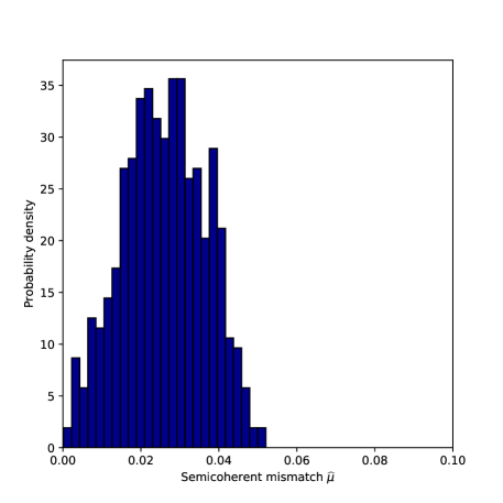
Figure 5: Distribution of semi-coherent mismatches $\hat{\mu}_{0}$ obtained from $500$ simulated 4D searches (left plot) over a small box in $f$, $a_{\mathrm{p}}$ and $t_{\mathrm{asc}}$ around the injected signals (with $P_{\mathrm{orb}}$ fixed at its injection value); and distribution of $500$ simulated 4D searches (right plot) over a small box in $f,a_{\mathrm{p}},t_{\mathrm{asc}}$ and $P_{\mathrm{orb}}$ around the injected signals, with parameters drawn randomly from the test range $\mathcal{P}_{0}$ defined in Table. 1. The template bank was constructed for a maximum mismatch of $\mu_{\max{}}=0.05$, with $N=120$ segments of $\Delta T=$3\text{\,}\mathrm{d}$$.

Search space $\mathcal{P}$	$f\,[$\mathrm{H}\mathrm{z}$]$	$a_{\mathrm{p}}\,[$\mathrm{l}\mathrm{s}$]$	$P_{\mathrm{orb}}\,[$\mathrm{s}$]$	$t_{\mathrm{asc}}\,[$\mathrm{G}\mathrm{P}\mathrm{S}\,\mathrm{s}$]$	Reference(s)/comment(s)
$\mathcal{P}_{0}$	10–700	0.3–3.5	68023.7 $\pm$ 0.2	1124044455.0 $\pm$ 1000	BinaryWeave test range
$\mathcal{P}_{1}$	20–500	1.26–1.62	68023.70496 $\pm$ 0.0432	897753994 $\pm$ 100	Leaci and Prix [36]
$\mathcal{P}_{2}$	60–650	1.45–3.25	68023.86048 $\pm$ 0.0432	974416624 $\pm$ 50	Abbott et al. [28]
$\mathcal{P}_{3}$	40–180	1.45–3.25	68023.86 $\pm$ 0.12	1178556229 $\pm$ 417	Zhang et al. [29]
$\mathcal{P}_{4}$	600–700
$\mathcal{P}_{5}$	1000–1100
$\mathcal{P}_{6}$	1400–1500	1.45–3.25	68023.70496 $\pm$ 0.0432	974416624 $\pm$ 100	different ranges in frequency
$\mathcal{P}_{7}$	20–250				with broad range in $a_{\mathrm{p}}$
$\mathcal{P}_{8}$	20–1000
$\mathcal{P}_{9}$	20–1500
$\mathcal{P}_{10}$	600–700
$\mathcal{P}_{11}$	1000–1100
$\mathcal{P}_{12}$	1400–1500	1.40–1.50	68023.70496 $\pm$ 0.0432	974416624 $\pm$ 100	different ranges in frequency
$\mathcal{P}_{13}$	20–500				with narrow range in $a_{\mathrm{p}}$
$\mathcal{P}_{14}$	20–1000
$\mathcal{P}_{15}$	20–1500
$\mathcal{P}_{16}$	600–700
$\mathcal{P}_{17}$	1000–1100
$\mathcal{P}_{18}$	1400–1500	1.44–1.45	68023.70496 $\pm$ 0.0432	974416624 $\pm$ 100	different ranges in frequency
$\mathcal{P}_{19}$	20–500				with well-constrained $a_{\mathrm{p}}$
$\mathcal{P}_{20}$	20–1000
$\mathcal{P}_{21}$	20–1500

Table 1: Different parameter space search regions considered for Sco X-1. $\mathcal{P}_{0}$ has been used in this study as a test range for various Monte-Carlo tests of BinaryWeave. $\mathcal{P}_{1-3}$ represent observational constraints considered in recent CW searches and studies. In addition, various combinations of parameter-ranges are considered, $\mathcal{P}_{4-21}$, in order to explore the impact of improved observation constraints and reduced search ranges.

Next we test the template-bank performance for the four possible combinations of three search parameters (3D searches) with the fourth one fixed to the signal injection parameter, as well as 4D searches over all four parameters $\{f,a_{\mathrm{p}},P_{\mathrm{orb}},t_{\mathrm{asc}}\}$. We perform several sets of simulations, using $\sim\mathcal{O}\left(100-1000\right)$ injections each, using varying search setups and maximum mismatch values $\mu_{\max{}}$, in order to obtain the resulting mismatch distribution of the template bank.

The injected signal parameters are randomly drawn from the test range $\mathcal{P}_{0}$ (cf. 1), namely $f\in[10,700]\,$\mathrm{H}\mathrm{z}$$ and binary parameter ranges wider than the Sco X-1 constraints, namely $a_{\mathrm{p}}\in[0.3-3.5]\,$\mathrm{l}\mathrm{s}$$, $P_{\mathrm{orb}}=$68\,023.7\pm 0.2\text{\,}\mathrm{s}$$ and $t_{\mathrm{asc}}=$1\,124\,044\,455.0\pm 1000\text{\,}\mathrm{G}\mathrm{P}\mathrm{S}\,\mathrm{s}$$.

Figure 3 shows an example for the mismatch distributions of coherent and semi-coherent mismatches obtained for a set of $1000$ injections and subsequent 3D searches in a small box around the injection in $f$, $a_{\mathrm{p}}$ and $t_{\mathrm{asc}}$, with $P_{\mathrm{orb}}$ fixed to the injected value. Figure 4 presents a corresponding example for the mismatch distributions obtained from $1000$ 4D box searches around the injected signals.

We see that the means of the coherent and semicoherent mismatch distributions are $\left\langle{{\mu}}\right\rangle\approx\left\langle{\hat{\mu}}\right\rangle\approx 0.17-0.18$, and the highest observed semicoherent mismatch in the 3D case is $\max{\hat{\mu}_{0}}\approx 0.4$, while in the 4D case it is $\max{\hat{\mu}_{0}}\approx 0.35$. This is smaller than the imposed maximum mismatch of $\mu_{\max{}}=0.5$, which is a common feature of the quadratic approximation Eq. (9) underlying the metric, namely the measured mismatch values $\mu_{0}$ tend to increasingly fall behind the predicted metric mismatch values with increasing mismatch [e.g., see 47, 56, 70]. Thus, in addition, we also test the metric mismatch implementations for small mismatch value $\mu_{\max{}}=0.05$ which is compareable to the realistic search setups relevant for Sco X-1 (discussed in details in Section V). We see a good agreement for both 3D and 4D template banks with such small $\mu_{\max{}}$ values as shown in Figure 5.

IV.3 Required computing resources

IV.3.1 Number of templates

As discussed in Sec. II.3, the bulk template count for a parameter space $\mathcal{P}$ (not counting any extra templates required for boundary padding of $\partial\mathcal{P}$) is given by Eq. 10.

Using the metric expressions in Eq. (14), this can be evaluated explicitly [36] and the bulk template count for 3D searches over $\{f,a_{\mathrm{p}},t_{\mathrm{asc}}\}$ is found as

$$\begin{split}\hat{\mathcal{N}}_{3\mathrm{D}}=\frac{\theta_{3}}{\mu_{\max{}}^{3/2}}\frac{\pi^{3}\Delta T}{\sqrt{27}}\,\Omega\,(f^{3}_{\max}-f^{3}_{\min})\,(a_{\mathrm{p}}^{2}{}_{,\max}-a_{\mathrm{p}}^{2}{}_{,\min})\\ \times(t_{\mathrm{asc}}{}_{,\max}-t_{\mathrm{asc}}{}_{,\min}),\end{split}$$ (26)

while for a 4D template bank over $\{f,a_{\mathrm{p}},P_{\mathrm{orb}},t_{\mathrm{asc}}\}$ one finds

$$\begin{split}\hat{\mathcal{N}}_{4\mathrm{D}}=\frac{\theta_{4}}{\mu_{\max{}}^{2}}\frac{\pi^{4}\gamma\Delta T^{2}}{36\sqrt{2}}(f_{\max}^{4}-f_{\min}^{4})(a_{\mathrm{p}}{}_{,\max}^{3}-a_{\mathrm{p}}{}_{,\min}^{3})\\ \times(\Omega_{\max}^{2}-\Omega_{\min}^{2})(t_{\mathrm{asc}}{}_{,\max}-t_{\mathrm{asc}}{}_{,\min}),\end{split}$$ (27)

where the coordinate ranges are $\lambda^{i}\in[\lambda^{i}_{\min},\lambda^{i}_{\max}]$, and $\gamma$ is the semi-coherent refinement factor associated with the $P_{\mathrm{orb}}$ (i.e., $\Omega$), given by

$$\gamma=\sqrt{1+12\frac{(\overline{\Delta}_{\mathrm{ma}}^{2}-\overline{\Delta_{\mathrm{ma}}^{2}})}{\Delta T^{2}}}.$$ (28)

The refinement factor evaluates to $\gamma=N$ in the case of segments without gaps. We can use these theoretical expressions to test against the actual number of templates generated by the BinaryWeave code, which includes boundary padding not accounted for in the above theoretical expressions.

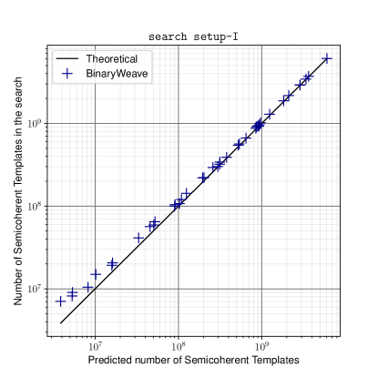
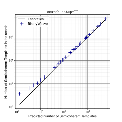
Figure 6: Number of semicoherent templates $\hat{\mathcal{N}}$ constructed by BinaryWeave versus with the theoretical bulk predictions of Eq. (27). Each point ‘$+$’ corresponds to a simulated 4D-box search around a randomly chosen parameter-space location in $\{f,a_{\mathrm{p}}\}\in\mathcal{P}_{0}$ (cf. Table 1 using either search setup-I (left plot) or search setup-II (right plot) defined in Table 2).

In the following we consider two example search setups (cf. Table 2), namely search setup-I with $N=180$ segments of duration $\Delta T=$1\text{\,}\mathrm{d}$$ and a maximum mismatch of $\mu_{\max{}}=0.031$, and search setup-II with $N=120$ segments of $\Delta T=$3\text{\,}\mathrm{d}$$ and maximum mismatch $\mu_{\max{}}=0.056$.

We generate a BinaryWeave template bank for a small box around a randomly-chosen point in $f$ and $a_{\mathrm{p}}$, drawn from the test range $\mathcal{P}_{0}$ of Table. 1. The box consist of $\mathcal{O}\left(${10}^{5}$\right)$ frequency bins and a metric bounding-box extent $D\lambda^{i}$ (cf. Eq. (12)) along each binary-orbital parameter dimension. This is repeated 40 times, in order to obtain a representative sampling over a wide range of search parameters, and the resulting BinaryWeave template counts are compared to the theoretical predictions of (27), shown in Fig. 6.

We see that there is generally good agreement in the template counts, with the real template counts exceeding the theoretical bulk predictions by factors up to $2-3$ at low template counts, with increasingly good agreement at higher template counts. The template counts exceeds only at the lowest frequency regime ($\leq 50$ Hz) by a factor of $\sim 2-3$, whereas agrees within $10\%$ at intermediate frequency ($\sim 200$ Hz) and $<5\%$ at higher frequency ($\sim 500$ Hz). This effect is expected from the extra padding required to fully cover the parameter-space boundaries $\partial\mathcal{P}$, which decreases in relative importance for increasing total template counts (i.e., boundary effects are less important for template spacings that are small compared to the parameter-space extents).

IV.3.2 Computing cost and memory usage

A detailed computing-cost (and memory) model exists for the semi-coherent Weave implementation [37] as well as for the underlying coherent $\mathcal{F}$-statistic implementation [71]. There are two different $\mathcal{F}$-statistic algorithms available, the resampling FFT algorithm (originally described in [43]), and the so-called demodulation algorithm introduced in [72, 69]. Because the resampling $\mathcal{F}$-statistic is substantially faster (i.e., $\mathcal{O}\left(100-1000\right)$) for large numbers of frequency bins (i.e., $\mathcal{O}\left(10^{5}\right)$) and SFTs, which is the relevant regime for the wide parameter-space search considered here, we will exclusively consider this algorithm for the following discussion of the Sco X-1 computing cost .

We performed the BinaryWeave tests and simulations on the LIGO Data Analysis System (LDAS) computing cluster at the LIGO Hanford Observatory, containing a combination of 2.4GHz Xeon E5-2630v3, 2.2GHz Xeon E5-2650v4, 3.5GHz Xeon E3-1240v5 and 3.0GHz Xeon Gold 6136 CPUs. We find the resulting semi-coherent timing coefficients measured on this hardware are essentially the same as given in Table. III of [37], while the effective (resampling-FFT) $\mathcal{F}$-statistic time per template and detector is observed to fall in the range $\tau_{\mathcal{F}}^{\mathrm{eff}}\approx(3.8-4.3)\times${10}^{-7}\text{\,}\mathrm{s}$$, consistent with the numbers obtained in [37].

We measure the CPU run-time per template $\mathcal{C}_{\mathrm{t}}$ and the maximum memory usage of BinaryWeave for the 80 box searches (two sets of 40 box searches each for setup-I and setup-II) described in the previous section (see Fig. 6). The maximum memory usage over all search boxes is found as $\sim$2.2\text{\,}\mathrm{G}\mathrm{B}$$, well below all-sky Weave numbers observed in [38], due to the fact that Sco X-1 has little refinement and we can use a non-interpolating search setup, substantially alleviating memory requirements.

The runtime per template $\mathcal{C}_{\mathrm{t}}$ is found to be relatively constant over the search parameter space and for the two search setups considered, namely $\mathcal{C}_{\mathrm{t}}(\texttt{search setup-I})\approx$0.12\pm 0.03\text{\,}\mathrm{ms}$$ and $\mathcal{C}_{\mathrm{t}}(\texttt{search setup-II})\approx$0.14\pm 0.03\text{\,}\mathrm{ms}$$. Here we only consider the non-interpolating StackSlide method, in which the coherent segments and the semi-coherent $\hat{\mathcal{F}}$-statistic share the same template grid and number of templates $\mathcal{N}$, i.e., ${\mathcal{N}}=\hat{\mathcal{N}}$. This implies that both the coherent and semi-coherent contributions to the total computing cost are proportional to $\mathcal{N}$. Therefore we can use a simplified effective model for the total computing cost $\mathcal{C}_{\mathcal{P}}$ over a search space $\mathcal{P}$ in the form

$$\mathcal{C}_{\mathcal{P}}=\mathcal{N}_{\mathcal{P}}\,\mathcal{C}_{\mathrm{t}},$$ (29)

where $\mathcal{N}_{\mathcal{P}}$ is the total number of templates covering the parameter space $\mathcal{P}$. Given the above timing measurements for the two setups, in the following we assume a (slightly conservative) effective CPU time per template of $\mathcal{C}_{\mathrm{t}}=$0.145\text{\,}\mathrm{m}\mathrm{s}$$. This simplified effective cost model is plotted against the measured BinaryWeave run times in Fig. 7.

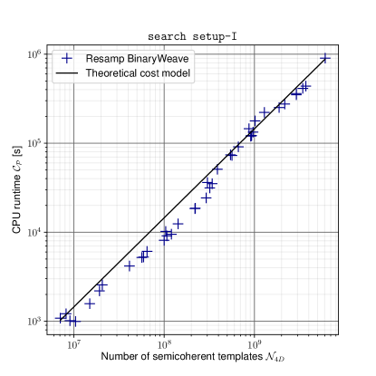
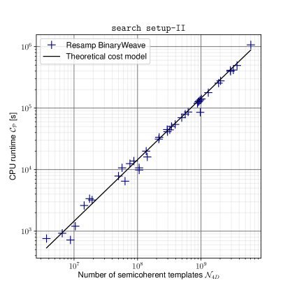
Figure 7: CPU run-time $\mathcal{C}_{\mathcal{P}}$ per search box as a function of the number of (semi-coherent) templates $\hat{\mathcal{N}}_{4\mathrm{D}}$ for that box, for search setup-I (left plot) and search setup-II (right plot), defined in Table. 2. The points ’$+$’ mark the measured BinaryWeave run times, while the solid line indicates the effective cost model prediction of Eq. (29), using an effective cost per template of $\mathcal{C}_{\mathrm{t}}=$0.145\text{\,}\mathrm{m}\mathrm{s}$$.

V Characterizing potential Sco X-1 searches

V.1 Sensitivity for different search setups

The sensitivity of a search is typically characterized by the weakest signal amplitude $h_{p_{\mathrm{fa}}}^{p_{\mathrm{det}}}$ detectable at a false-alarm probability $p_{\mathrm{fa}}$ with detection probability (or “confidence level”) $p_{\mathrm{det}}$. While this is astrophysically informative, for a given search method it is often more instructive [74] to use the sensitivity depth $0pt_{p_{\mathrm{fa}}}^{p_{\mathrm{det}}}$ instead, defined as

$$0pt_{p_{\mathrm{fa}}}^{p_{\mathrm{det}}}\equiv\frac{\sqrt{S_{\mathrm{n}}}}{h_{p_{\mathrm{fa}}}^{p_{\mathrm{det}}}},$$ (30)

which characterizes the sensitivity of a method independently of the noise floor (i.e., power spectral density) $S_{\mathrm{n}}$.

As discussed in [75, 74], the sensitivity of a semi-coherent StackSlide $\hat{\mathcal{F}}$-statistic search can be estimated quite accurately (to better than $\sim$10\text{\,}\mathrm{\char 37\relax}$$) given the total amount of data used, the number $N$ of semi-coherent segments and the mismatch distribution of the template bank. This algorithm is implemented in the OctApps [76] function SensitivityDepthStackSlide().

For each search setup listed in Table. 2 we obtain the mismatch distribution empirically by injection-recovery Monte-Carlo simulation (cf. Sec. IV.2.2), and use this to estimate the expected sensitivity depth for each setup. We use a canonical value of $p_{\mathrm{fa}}=${10}^{-10}$$ (as was done in [36]) for the single-template false-alarm probability, which represents a somewhat typical false-alarm scale for wide parameter-space searches. We quote the sensitivity depth for $p_{\mathrm{det}}=$90\text{\,}\mathrm{\char 37\relax}$,$95\text{\,}\mathrm{\char 37\relax}$$ and $99\text{\,}\mathrm{\char 37\relax}$. The former two are typical confidence-levels used for upper limits obtained in CW searches, while the last one might be interesting, for example, if one is interested in rejecting the torque-balance hypothesis or a specific emission mechanism in some parameter range at high confidence.

In Table 2, we summarize the sensitivity depths for a set of six different search setups. The sensitivity depths obtained from the empirical mismatch distributions corresponding to the well-studied setup-I and setup-II are presented in this table. In addition, we report the maximum achievable sensitivity depths for this BinaryWeave pipeline estimated from our simulated searches for four different setups that may be relevant for different cases of unknown spin wandering effect in Sco X-1.

Search setup	$T_{\mathrm{obs}}$	$\Delta T$	$N$	$\mu_{\max{}}$	$0pt_{p_{\mathrm{fa}}}^{90\%}$	$0pt_{p_{\mathrm{fa}}}^{95\%}$	$0pt_{p_{\mathrm{fa}}}^{99\%}$
	$[$\mathrm{m}\mathrm{o}\mathrm{n}\mathrm{t}\mathrm{h}\mathrm{s}$]$	$[$\mathrm{d}\mathrm{a}\mathrm{y}\mathrm{s}$]$			$[$\mathrm{1}\mathrm{/}\sqrt{\mathrm{Hz}}$]$	$[$\mathrm{1}\mathrm{/}\sqrt{\mathrm{Hz}}$]$	$[$\mathrm{1}\mathrm{/}\sqrt{\mathrm{Hz}}$]$
search setup-I	6	1	180	0.031	77	72	60
search setup-II	12	3	120	0.056	116	107	91
search setup-III	6	3	60	0.025	96	89	75
search setup-IV	12	1	360	0.025	93	86	73
search setup-V	6	10	18	0.025	120	111	94
search setup-VI	12	10	36	0.025	150	138	117

Table 2: Definition of example search setups with corresponding estimated sensitivity depth, discussed in Sec. V.1. The sensitivity estimates assume a (per-template) false-alarm probability of $p_{\mathrm{fa}}=${10}^{-10}$$ and detection confidences $p_{\mathrm{det}}=90\%,95\%,\text{and}\,99\%$, respectively, using the measured (4D) mismatch distributions obtained for each setup (cf. Sec. IV.2.2).

V.2 Computing cost for different search scenarios

	(I,3D)	(I,4D)	(II,3D)	(II,4D)
$\mathcal{P}_{1}$	3.18	23.51	3.93	43.23
$\mathcal{P}_{2}$	28.50	466.48	35.22	857.69
$\mathcal{P}_{3}$	5.00	63.40	6.17	116.57
$\mathcal{P}_{4}$	26.38	577.57	32.60	1061.95
$\mathcal{P}_{5}$	68.76	2425.79	84.96	4460.17
$\mathcal{P}_{6}$	131.09	6381.48	161.97	11733.30
$\mathcal{P}_{7}$	3.24	20.42	4.01	37.54
$\mathcal{P}_{8}$	207.74	5226.87	256.69	9610.37
$\mathcal{P}_{9}$	701.14	26461.02	866.33	48652.49
$\mathcal{P}_{10}$	0.90	11.65	1.12	21.42
$\mathcal{P}_{11}$	2.36	48.94	2.91	89.97
$\mathcal{P}_{12}$	4.49	128.73	5.55	236.70
$\mathcal{P}_{13}$	0.11	0.41	0.14	0.76
$\mathcal{P}_{14}$	7.12	105.44	8.80	193.87
$\mathcal{P}_{15}$	24.03	533.80	29.70	981.46
$\mathcal{P}_{16}$	0.09	1.16	0.11	2.13
$\mathcal{P}_{17}$	0.23	4.86	0.29	8.93
$\mathcal{P}_{18}$	0.45	12.78	0.55	23.50
$\mathcal{P}_{19}$	0.01	0.04	0.01	0.08
$\mathcal{P}_{20}$	0.71	10.47	0.88	19.25
$\mathcal{P}_{21}$	2.40	52.99	2.96	97.43

Table 3: Computing-cost estimates $\mathcal{C}_{\mathcal{P}}$ (in million core hours [Mh]) for different parameter spaces $\mathcal{P}_{n}$ defined in Table. 1. We consider two setups, search setup-I and search setup-II of Table 2, assuming either a 3D or 4D template-bank.

Here we present CPU computing cost in terms of core hours, and million core hours (Mh), referring to the mix of CPU hardware used in the present study, cf. Sec. IV.3.2. Another interesting unit used in [36] is Einstein@Home months (EM), which was defined as $12\,000$ (average) CPU cores running on Einstein@Home [39] for 30 days. If one assumes the (current) average Einstein@Home CPU to be roughly comparable to the one used here, one can convert $$1\text{\,}\mathrm{E}\mathrm{M}$\approx$8.6\text{\,}\mathrm{M}\mathrm{h}$$.

Let us first consider the example of the Sco X-1 parameter space $\mathcal{P}_{1}$ considered in Leaci and Prix [36] (cf. Table 1) with two different search setups (I and II) of Table. 2. For search setup-I with $180\times$1\text{\,}\mathrm{d}$$ segments and mismatch $\mu_{\max{}}=0.031$, the total number of (4D) templates given by Eq. (27) is $\mathcal{N}_{4\mathrm{D}}=$5.84\text{\times}{10}^{14}$$. Using the effective computing-cost model of Eq. (29) this results in a total CPU runtime of $\mathcal{C}_{\mathcal{P}_{1}}[\texttt{search setup-I}]\approx$8.46\text{\times}{10}^{10}\text{\,}\mathrm{s}$=$23.5\text{\,}\mathrm{M}\mathrm{h}$$. Using the above conversion factors, this would correspond to $2.7\text{\,}\mathrm{E}\mathrm{M}$. Similarly, for search setup-II with $120\times$3\text{\,}\mathrm{d}$$ segments and mismatch of $\mu_{\max{}}=0.056$, we obtain a template count of $\mathcal{N}_{4\mathrm{D}}=$1.07\text{\times}{10}^{15}$$ and a corresponding total CPU runtime of $\mathcal{C}_{\mathcal{P}_{1}}[\texttt{search setup-II}]\approx$1.56\text{\times}{10}^{11}\text{\,}\mathrm{s}$=$43.2\text{\,}\mathrm{M}\mathrm{h}$$, which we can also express as $5.0\text{\,}\mathrm{E}\mathrm{M}$.

Next we consider a number of additional parameter-space scenarios, listed in Table. 1. The constraints from optical and radio emission observations come from different sources in the literature [18, 62], with the most recent values given in [77, 63]. Future observations are likely to further alter and improve these constraints. For a fully-resolved period uncertainty, the total number of templates (and therefore computing cost) scales as $a_{\mathrm{p}}{}_{\max}^{3}$ for a wide parameter uncertainty in $a_{\mathrm{p}}$ (cf. Eq. (27)), but only as $a_{\mathrm{p}}{}_{\max}^{2}\,\Delta a_{\mathrm{p}}$ for narrow parameter uncertainty $\Delta a_{\mathrm{p}}$.

In order to quantify the effects of future improved constraints on $a_{\mathrm{p}}$, we consider three different scenarios: (i) $a_{\mathrm{p}}\in[1.45,3.25]\,$\mathrm{l}\mathrm{s}$$ (search spaces $\mathcal{P}_{4}-\mathcal{P}_{9}$), (ii) $a_{\mathrm{p}}\in[1.40,1.50]\,$\mathrm{l}\mathrm{s}$$ (search spaces $\mathcal{P}_{10}-\mathcal{P}_{15}$) and (iii) $a_{\mathrm{p}}\in[1.44,1.45]\,$\mathrm{l}\mathrm{s}$$ (search spaces $\mathcal{P}_{16}-\mathcal{P}_{21}$). Similarly we consider six different frequency search ranges, three “deep-search” ranges covering only $100\text{\,}\mathrm{H}\mathrm{z}$ at different frequencies ($600700\text{\,}\mathrm{H}\mathrm{z}$, $10001100\text{\,}\mathrm{H}\mathrm{z}$, and $14001500\text{\,}\mathrm{H}\mathrm{z}$), and three “broad-search” ranges within the LIGO/Virgo frequency band ($20500\text{\,}\mathrm{H}\mathrm{z}$, $201000\text{\,}\mathrm{H}\mathrm{z}$ and $201500\text{\,}\mathrm{H}\mathrm{z}$). Finally, we consider both a 3D (for an unresolved period uncertainty $\Delta P_{\mathrm{orb}}$) and 4D search for all cases considered.

The resulting computing cost estimates for all combinations of the two setups (I and II), 3D or 4D template bank, and different parameter spaces $\mathcal{P}_{1-21}$ are given in Table. 3. We note that while some required computing budgets may seem unrealistically large, a recent GPU port of the $\mathcal{F}$-statistic and Weave [73, 57] may yield speedups factors of tens to hundreds, making many more setups fall within reach of currently available computing resources.

V.3 Sensitivity versus computing cost

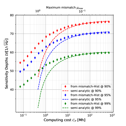
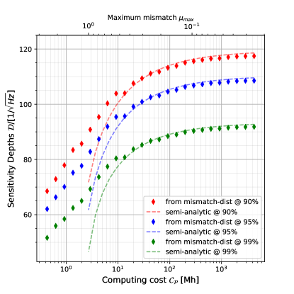
Figure 8: Sensitivity depth $0pt_{p_{\mathrm{fa}}}^{p_{\mathrm{det}}}$ as a function of (4D) computing cost $\mathcal{C}_{\mathcal{P}}$ for varying maximum mismatch $\mu_{\max{}}$ at fixed segments ($N,\Delta T$), assuming Sco X-1 parameter space $\mathcal{P}_{2}$ of Table 1. Sensitivity depth is estimated for a fixed (per-template) false-alarm of $p_{\mathrm{fa}}=${10}^{-10}$$ and different confidence levels of $p_{\mathrm{det}}=$90\text{\,}\mathrm{\char 37\relax}$$ (top), $p_{\mathrm{det}}=$95\text{\,}\mathrm{\char 37\relax}$$ (middle) and $p_{\mathrm{det}}=$99\text{\,}\mathrm{\char 37\relax}$$ (bottom). Segment setup is $N\times\Delta T=180\times$1\text{\,}\mathrm{d}$$ (left plot), and $120\times$3\text{\,}\mathrm{d}$$ (right plot), corresponding to search setup-I and search setup-II, respectively (cf. Table 2). The dashed lines correspond to the sensitivity estimate assuming a theoretical $A_{n}^{*}$ lattice mismatch-distribution, while the diamond markers correspond to using the measured BinaryWeave mismatch distributions. Computing cost is measured in million core hours (Mh).

In addition to considering various fixed search scenarios as in the previous two subsections, it is also instructive to study how the achievable sensitivity varies as a function of the invested computing cost. This would generally involve a (3- or 4-dimensional) optimization problem over all search-setup parameters (see [40, 36]) which is beyond the scope of this study, so we consider a simpler problem of varying the maximal template-bank mismatch $\mu_{\max{}}$. In a sense, this provides a lower limit on the achievable sensitivity at any given cost, as one could always improve sensitivity further by varying all three setup parameters $\{\mu_{\max{}},N,\Delta T\}$ at fixed cost.

The search space is chosen as $\mathcal{P}_{2}$, and we use again search setup-I (i.e., $180\times$1\text{\,}\mathrm{d}$$ segments) and search setup-II (i.e., $180\times$3\text{\,}\mathrm{d}$$) as baselines, but now we vary the maximal template-bank mismatch in the range $0.025\leq\mu_{\max{}}\leq 2.5$. For each mismatch, we can estimate the number of templates $\mathcal{N}_{4D}\propto\mu_{\max{}}^{-2}$ via Eq. (27), and obtain the corresponding computing cost $\mathcal{C}$ from the simplified cost model Eq. (29). We use the corresponding theoretical mismatch distribution for the $A_{n}^{*}$-lattice, as well as the measured distribution from a set of $100$ injection-recovery simulations using BinaryWeave, to estimate the expected sensitivity depth via SensitivityDepthStackSlide() from OctApps.

This allows us to plot sensitivity depth versus computing cost, parametrized along $\mu_{\max{}}$ at fixed segment setup $N\times\Delta T$, which is shown in Fig. 8. As expected, sensitivity improves as the invested computational cost increases and (equivalently) the maximum mismatch decreases; for $\mu_{\max{}}\lesssim 0.1$, however, further gains in sensitivity are minimal. We observe good agreement at small mismatches (i.e., large computing costs) between the theoretical estimates (using expected lattice mismatch distributions) and estimates using the measured mismatch distributions. The small loss of the measured versus expected sensitivity in this regime from (well known) additional intrinsic losses ($\sim\mathcal{O}\left($13\text{\,}\mathrm{\char 37\relax}$\right)$) of the high-performance $\mathcal{F}$-statistic implementation compared to the exact calculation. At higher mismatches $\mu_{\max{}}$, the measured mismatches tend to be smaller than the metric predictions, due to neglected higher-order terms in the metric approximation, as discussed previously in Sec. II.3 and Sec. IV.2.2. This explains the measured sensitivity decreasing more slowly compared to the theoretical estimates at higher mismatches (i.e., smaller computing cost).

VI Summary and outlook

In this paper, we presented the implementation and characterization of BinaryWeave, a new semi-coherent search pipeline for CWs from neutron stars in binary systems with known sky-position. This pipeline is based on the Weave framework [37], initially developed for all-sky searches of isolated sources, using the well established semi-coherent StackSlide $\hat{\mathcal{F}}$-statistic.

The Weave framework requires a constant metric over the search parameter space for lattice tiling, and in order to apply the non-constant binary metric of Leaci and Prix [36], we needed to develop a new internal coordinate system in which a constant approximation to the binary metric can be obtained. This is the basis for the BinaryWeave implementation. We performed extensive Monte-Carlo tests for the safety (in terms of mismatches) of the resulting template banks and their template counts versus theoretical model expectations. Furthermore, we obtained a simplified timing model for the non-interpolating StackSlide mode used here, which allows easy estimates for the required computing cost of a given search, based on the known analytic template-count models.

Putting these pieces together, we illustrate expected sensitivity depths for BinaryWeave assuming different search setups, and we estimate the corresponding required computing costs for a number of different Sco X-1 parameter-space regions of interest.

Two other primary pipelines, CrossCorr and Viterbi, are presently used for searching CW-signals from Sco X-1. Viterbi pipeline aims to track the stochastic phase evolution model due to spin-wandering effect of the neutron star in Sco X-1. It is thus more robust against this effect. The computational cost is also quite less compared to the most sensitive searches of BinaryWeave. However, the maximum achievable sensitivity depth for Viterbi is also less as compared to the most sensitive search of BinaryWeave provided the spin-wandering effect is not significantly large.

The sensitivity of CrossCorr pipeline is expected to be comparable to BinaryWeave. The computing cost for resampling CrossCorr is also expected to be comparable to BinaryWeave. However, BinaryWeave can be adopted to utalize different grid spacing for coherent and semi-coherent template banks that can reduce the computing cost for a search. This extra amount of computing resource can be reutilized to further increase the sensitivity depth of BinaryWeave by either decreasing the mismatch or increasing the segment lengths.

One of the primary goals of developing BinaryWeave is to perform searches for Sco X-1 that can beat the torque-balance limit over as wide a frequency range as possible, and are able to take advantage of any large available computing budget. Still, at the current level of electromagnetic constraints on the Sco X-1 parameters, reaching the torque-balance limit over the full frequency range remains computationally prohibitive. Future improvements in these constraints will be immensely impactful to increase the chances of detecting a CW signal from Sco X-1 (or other LMXBs), as illustrated in Sec. V.2.