Flow in Porous Media with Fractures of Varying Aperture

Abstract

We study single-phase flow in a fractured porous medium at a macroscopic scale that allows to model fractures individually. The flow is governed by Darcy’s law in both fractures and porous matrix. We derive a new mixed-dimensional model, where fractures are represented by $(n-1)$-dimensional interfaces between $n$-dimensional subdomains for $n\geq 2$. In particular, we suggest a generalization of the model in [22] by accounting for asymmetric fractures with spatially varying aperture. Thus, the new model is particularly convenient for the description of surface roughness or for modeling curvilinear or winding fractures. The wellposedness of the new model is proven under appropriate conditions. Further, we formulate a discontinuous Galerkin discretization of the new model and validate the model by performing two- and three-dimensional numerical experiments.

76S05, 35J20, 35J25, 65N30

1 Introduction

In many situations, the fluid flow in a porous medium is significantly influenced, if not dominated, by the presence of fractures. Fractures are characterized by an extreme geometry with a thin aperture but wide extent in the remaining directions of space. Hence, they form narrow heterogeneities that pose a challenge for classical continuum modeling. We assume that fractures are filled by another porous medium (e.g., debris) whose hydraulic properties may differ considerably from those of the surrounding porous matrix. Depending on the permeability inside a fracture, the fracture may serve as primary transport path for the overall flow in a porous medium or, conversely, may act as an almost impermeable barrier.

Fluid flow in fractured porous media is of essential relevance for a wide range of applications, such as geothermal energy, enhanced oil recovery, groundwater flow, nuclear waste disposal, and carbon sequestration. In the last decades, a diversity of mathematical models for fluid flow in fractured porous media has been developed. For a current review of modeling and discretization approaches, we refer to [6] and the literature therein. Besides, for a comparison of numerical methods and benchmark test cases for single-phase flow in fractured porous media, we refer to [7, 12, 15].

A common macroscopic modeling approach for flow in fractured porous media is to consider a reduced representation where fractures are described explicitly as $(n-1)$-dimensional interfaces between $n$-dimensional bulk domains [1, 3, 8, 13, 14, 16, 19, 20, 21, 22, 23]. In contrast to a full-dimensional representation of fractures, this avoids thin equi-dimensional subdomains which require highly resolved grids in numerical methods. Typically, these kinds of interface models are based on the idealized conception of a planar fracture geometry with constant aperture. However, in this case, the resulting reduced model cannot account for surface roughness and does not properly describe curvilinear or winding fractures. Thus, more generally, the geometry of a fracture may be described by spatially varying aperture functions, which is the approach that we follow here.

Specifically, we consider single-phase fluid flow in a fractured porous medium governed by Darcy’s law. We suggest a new mixed-dimensional model that accounts for asymmetric fractures with spatially varying aperture and, thereby, propose an extension and alternative derivation of the model in the seminal work in [22] that was derived for fractures with constant aperture. For the derivation of the new fracture-averaged model, we proceed from a domain-decomposed system for Darcy’s flow with full-dimensional fracture that closely resembles the initial model in [22]. However, as a central issue when dealing with a spatially varying fracture aperture, the normal vectors at the internal boundaries of the initial full-dimensional fracture depend on aperture gradients and are generally not aligned with the normal vector of the interfacial fracture in the desired reduced model. In contrast to the approach in [22], we address this problem by employing a weak formulation when averaging across the fracture and by approximating suitable curve integrals across the fracture to obtain internal boundary conditions.

Section 2 introduces an initial model problem with full-dimensional fracture in a weak formulation. In Section 3, we derive a new reduced model with interfacial fracture that accounts for a spatially varying aperture. The resulting reduced model is summarized and discussed in Section 4, where we also introduce four related model variants. Section 5 introduces a discontinuous Galerkin (DG) discretization of the new model. Numerical results are presented in Section 6.

2 Darcy Flow with Full-Dimensional Fracture

Let $\Omega\subset\mathbb{R}^{n}$ be a bounded Lipschitz domain that is occupied by an $n$-dimensional porous medium, where $n\in\mathbb{N}$ with $n\geq 2$. We suppose that the flow of a single-phase fluid in $\Omega$ is governed by Darcy’s law and mass conservation, i.e.,

(1a) $$-\nabla\cdot\mathopen{}\mathclose{{}\left(\mathbf{K}\nabla p}\right) =q\qquad \text{in }\Omega,$$

(1b) $$p =0\qquad \text{on }\partial\Omega.$$

In Eq. 1, $p\colon\Omega\rightarrow\mathbb{R}$ is the pressure and $q\in L^{2}(\Omega)$ denotes the source term. The permeability matrix is denoted by $\mathbf{K}\in L^{\infty}(\Omega;\mathbb{R}^{n\times n})$ and required to be symmetric and uniformly elliptic. The choice of homogeneous Dirichlet boundary conditions is only made for the sake of simplicity. A weak formulation of the Darcy system (1) is given by the following problem. Find $p\in H^{1}_{0}\mathopen{}\mathclose{{}\left(\Omega}\right)$ such that

(2) $$\int_{\Omega}\mathbf{K}\nabla p\cdot\nabla\varphi\,\mathrm{d}V =\int_{\Omega}q\varphi\,\mathrm{d}V\qquad\text{for all }\varphi\in H^{1}_{0}\mathopen{}\mathclose{{}\left(\Omega}\right).$$

We consider the case of a single fracture as an $n$-dimensional open subdomain $\Omega_{\mathrm{f}}\subset\Omega$ crossing the entire domain $\Omega$ such that $\Omega$ is cut into two disjoint connected subdomains $\Omega_{1}$ and $\Omega_{2}$, i.e., $\Omega\setminus\overline{\Omega}_{\mathrm{f}}=\Omega_{1}\>\dot{\cup}\>\Omega_{2}$. Moreover, we suppose that the fracture domain $\Omega_{\mathrm{f}}$ can be parameterized by a hyperplane $\Gamma$ and two functions $d_{1},d_{2}\in W^{1,\infty}(\Gamma)$ which describe the aperture of the fracture on the left and right side of $\Gamma$ such that

(3) $$\Omega_{\mathrm{f}}=\big{\{}{\bm{\gamma}}+\lambda{\bm{n}}\in\Omega\ \big{|}\ {\bm{\gamma}}\in\Gamma,\,\lambda\in\mathopen{}\mathclose{{}\left(-d_{1}\mathopen{}\mathclose{{}\left({\bm{\gamma}}}\right),d_{2}\mathopen{}\mathclose{{}\left({\bm{\gamma}}}\right)}\right)\big{\}}.$$

In Eq. 3, ${\bm{n}}$ denotes the unit normal of the hyperplane $\Gamma$ that points in the direction of $\Omega_{2}$. Further, we write $d:=d_{1}+d_{2}>0$ for the total aperture of the fracture. We only require the total aperture $d$ to be positive, not the functions $d_{1}$ and $d_{2}$, so that the hyperplane $\Gamma$ is not necessarily required to be fully immersed inside the fracture domain $\Omega_{\mathrm{f}}$. This allows the description of curvilinear or winding fractures in a natural way. Besides, w.l.o.g., the hyperplane $\Gamma$ is represented by $\Gamma=\mathopen{}\mathclose{{}\left\{{\bm{x}}\in\Omega\ \middle|\ {\bm{n}}\cdot{\bm{x}}=0}\right\}$. In addition, we denote by $\varrho_{i}:=\partial\Omega_{i}\cap\partial\Omega$ the exterior boundary of the overall domain $\Omega$ inside $\Omega_{i}$ for $i\in\mathopen{}\mathclose{{}\left\{1,2,\mathrm{f}}\right\}$ and by $\Gamma_{i}:=\partial\Omega_{i}\cap\partial{\Omega_{\mathrm{f}}}$ the interface between the bulk domain $\Omega_{i}$ and the fracture domain $\Omega_{\mathrm{f}}$ for $i\in\mathopen{}\mathclose{{}\left\{1,2}\right\}$.

Figure 1: Sketch of the geometry for the full-dimensional Darcy problem (5).

The specified geometric situation is sketched in Figure 1. We remark that, for the representation of the fracture in Eq. 3, it is required that the connecting lines between the interfaces $\Gamma_{1}$ and $\Gamma_{2}$ along ${\bm{n}}$ exist and are contained in the fracture domain $\Omega_{\mathrm{f}}$.

Next, for $i\in\mathopen{}\mathclose{{}\left\{1,2,\mathrm{f}}\right\}$ and functions $f\colon\Omega\rightarrow B$ and $\bar{f}\colon\partial\Omega\rightarrow B$ with arbitrary codomain $B$, we introduce the notation

(4) $$f_{i}:={\mathopen{}\mathclose{{}\left.\kern-1.2ptf\vphantom{\big{|}}}\right|_{\Omega_{i}}}\quad\text{and}\quad\bar{f}_{i}:={\mathopen{}\mathclose{{}\left.\kern-1.2pt\bar{f}\vphantom{\big{|}}}\right|_{\varrho_{i}}}.$$

Following a domain decomposition approach, this allows us to reformulate (1) as

(5a) $$-\nabla\cdot\mathopen{}\mathclose{{}\left(\mathbf{K}_{i}\nabla p_{i}}\right) =q_{i}\qquad \text{in }\Omega_{i},\quad i\in\mathopen{}\mathclose{{}\left\{1,2,\mathrm{f}}\right\},$$

(5b) $$p_{i} =0\qquad \text{on }\varrho_{i},\quad i\in\mathopen{}\mathclose{{}\left\{1,2,\mathrm{f}}\right\},$$

(5c) $$p_{i} =p_{\mathrm{f}}\qquad \text{on }\Gamma_{i},\quad i\in\mathopen{}\mathclose{{}\left\{1,2}\right\},$$

(5d) $$\mathbf{K}_{i}\nabla p_{i}\cdot{\bm{n}}_{i} =\mathbf{K}_{\mathrm{f}}\nabla p_{\mathrm{f}}\cdot{\bm{n}}_{i}\qquad \text{on }\Gamma_{i},\quad i\in\mathopen{}\mathclose{{}\left\{1,2}\right\}.$$

Here, for $i\in\mathopen{}\mathclose{{}\left\{1,2}\right\}$, we denote by ${\bm{n}}_{i}$ the unit normal to the interface $\Gamma_{i}$ that points into the bulk domain $\Omega_{i}$. The vectors ${\bm{n}}_{1}$ and ${\bm{n}}_{2}$ are given by

(6) $${\bm{n}}_{1}=\frac{-{\bm{n}}-\nabla d_{1}}{\sqrt{1+{\mathopen{}\mathclose{{}\left|\nabla d_{1}}\right|}^{2}}},\qquad{\bm{n}}_{2}=\frac{{\bm{n}}-\nabla d_{2}}{\sqrt{1+{\mathopen{}\mathclose{{}\left|\nabla d_{2}}\right|}^{2}}}.$$

Next, we set up a weak formulation for the domain-decomposed Darcy problem in Eq. 5. For $i\in\{1,2,\mathrm{f}\}$, we define the space $V_{i}$ by

(7) $$V_{i} :=\mathopen{}\mathclose{{}\left\{p_{i}\in H^{1}_{0,\varrho_{i}}(\Omega_{i})\ \middle|\ \mathbf{K}_{i}\nabla p_{i}\in H_{\mathrm{div}}(\Omega_{i})}\right\}.$$

Further, with $H_{\mathrm{div}}(\Omega_{i}):=\{{\bm{w}}\in L^{2}(\Omega_{i};\mathbb{R}^{n})\,|\,\nabla\cdot{\bm{w}}\in L^{2}(\Omega_{i})\}$ and $H^{1}_{0,\varrho_{i}}(\Omega_{i}):=\{f\in H^{1}(\Omega_{i})\,|\,f=0\text{ on }\varrho_{i}\}$ for $i\in\{1,2,\mathrm{f}\}$, we define the domain-decomposed spaces

(8) $$\begin{split}V_{\mathrm{dd}}&:=\big{\{}\mathopen{}\mathclose{{}\left(p_{1},p_{2},p_{\mathrm{f}}}\right)\in\bigtimes\nolimits_{i=1,2,\mathrm{f}}V_{i}\ \big{|}\ p_{i}=p_{\mathrm{f}}\text{ a.e. on }\Gamma_{i},\;i\in\mathopen{}\mathclose{{}\left\{1,2}\right\}\big{\}},\end{split}$$

(9) $$\Phi_{\mathrm{dd}} :=\bigtimes\nolimits_{i=1,2,\mathrm{f}}H^{1}_{0,\varrho_{i}}\mathopen{}\mathclose{{}\left(\Omega_{i}}\right).$$

Then, a weak formulation of the domain-decomposed Darcy problem (5) is given by the following problem. Find $p=\mathopen{}\mathclose{{}\left(p_{1},p_{2},p_{\mathrm{f}}}\right)\in V_{\mathrm{dd}}$ such that

(10) $$\mathcal{B}_{\mathrm{dd}}\mathopen{}\mathclose{{}\left(p,\varphi}\right) =\mathcal{L}_{\mathrm{dd}}\mathopen{}\mathclose{{}\left(\varphi}\right)\qquad\text{for all }\varphi=\mathopen{}\mathclose{{}\left(\varphi_{1},\varphi_{2},\varphi_{\mathrm{f}}}\right)\in\Phi_{\mathrm{dd}}.$$

In Eq. 10, given $p=\mathopen{}\mathclose{{}\left(p_{1},p_{2},p_{\mathrm{f}}}\right)\in V_{\mathrm{dd}}$ and $\varphi=\mathopen{}\mathclose{{}\left(\varphi_{1},\varphi_{2},\varphi_{\mathrm{f}}}\right)\in\Phi_{\mathrm{dd}}$, the bilinear form $\mathcal{B}_{\mathrm{dd}}\colon V_{\mathrm{dd}}\times\Phi_{\mathrm{dd}}\rightarrow\mathbb{R}$ and the linear form $\mathcal{L}_{\mathrm{dd}}\colon\Phi_{\mathrm{dd}}\rightarrow\mathbb{R}$ are defined by

(11a) $$\begin{split}\mathcal{B}_{\mathrm{dd}}\mathopen{}\mathclose{{}\left(p,\varphi}\right)&:=\smash{\sum_{i=1,2,\mathrm{f}}}\int_{\Omega_{i}}\mathbf{K}_{i}\nabla p_{i}\cdot\nabla\varphi_{i}\,\mathrm{d}V-\sum_{i=1,2}\int_{\Gamma_{i}}\big{[}\varphi_{\mathrm{f}}-\varphi_{i}\big{]}\mathbf{K}_{i}\nabla p_{i}\cdot{\bm{n}}_{i}\,\mathrm{d}\sigma,\end{split}$$

(11b) $$\mathcal{L}_{\mathrm{dd}}\mathopen{}\mathclose{{}\left(\varphi}\right) :=\sum_{i=1,2,\mathrm{f}}\int_{\Omega_{i}}q_{i}\varphi_{i}\,\mathrm{d}V.$$

Moreover, we state the following result, which is often used in the context of domain decomposition methods. For a proof, we refer to [17].

Theorem 2.1.

1. Let $p\in H_{0}^{1}(\Omega)$ be a weak solution of the single-domain Darcy problem (2). Then, $\mathopen{}\mathclose{{}\left(p_{1},p_{2},p_{\mathrm{f}}}\right)\in V_{\mathrm{dd}}$ is a weak solution of the domain-decomposed Darcy problem (10).

2. Conversely, let $\big{(}p^{(1)},p^{(2)},p^{(\mathrm{f})}\big{)}\in V_{\mathrm{dd}}$ be a weak solution of the domain-decomposed Darcy problem (10). Then, the function $p\in H^{1}_{0}\mathopen{}\mathclose{{}\left(\Omega}\right)$ defined by

   (12) $$p\mathopen{}\mathclose{{}\left({\bm{x}}}\right) :=\begin{cases}p^{(i)}\mathopen{}\mathclose{{}\left({\bm{x}}}\right)&\text{if }{\bm{x}}\in\Omega_{i},\enspace i\in\{1,2,\mathrm{f}\}\\ \end{cases}$$

   is a weak solution of the single-domain Darcy problem (2).

In particular, the problem (10) has a unique weak solution $\mathopen{}\mathclose{{}\left(p_{1},p_{2},p_{\mathrm{f}}}\right)\in V_{\mathrm{dd}}$.

3 Derivation of a Reduced Model

Proceeding from the weak domain-decomposed Darcy problem (10), we will derive a new reduced model in which the fracture cutting the domain $\Omega$ is solely described by the hyperplane $\Gamma$ between the two bulk subdomains $\Omega_{1}$ and $\Omega_{2}$. The new reduced model (56) is obtained by introducing fracture-averaged effective quantities, splitting integrals over $\Omega_{\mathrm{f}}$ into a surface integral over $\Gamma$ and a line integral in normal direction, and transforming integrals over the interfaces $\Gamma_{i}$ into integrals over $\Gamma$. In addition, two boundary conditions on $\Gamma$ are found by approximating curve integrals across the fracture domain $\Omega_{\mathrm{f}}$ using a quadrature rule and polynomial interpolation. Besides, the following result on the weak differentiation of parameter integrals will be useful.

Lemma 3.1 (Weak Leibniz Rule).

For $i\in\mathopen{}\mathclose{{}\left\{1,2}\right\}$, let $a_{i},b_{i}\in\mathbb{R}$ with $a_{i}<b_{i}$ and $I_{i}:=\mathopen{}\mathclose{{}\left(a_{i},b_{i}}\right)$. Further, let $f\in W^{1,p}\mathopen{}\mathclose{{}\left(I_{1}\times I_{2}}\right)$ and $\chi,\psi\in W^{1,\infty}\mathopen{}\mathclose{{}\left(I_{2}}\right)\cap W^{2,q}\mathopen{}\mathclose{{}\left(I_{2}}\right)$ such that $\chi\mathopen{}\mathclose{{}\left(I_{2}}\right),\psi\mathopen{}\mathclose{{}\left(I_{2}}\right)\subset I_{1}$ (except for null sets), where $p,q\in(1,\infty)$ with $\frac{1}{p}+\frac{1}{q}=1$. Then, the function $\smash{I_{2}\rightarrow\mathbb{R},\ y\mapsto\int_{\chi\mathopen{}\mathclose{{}\left(y}\right)}^{\psi\mathopen{}\mathclose{{}\left(y}\right)}\!f\mathopen{}\mathclose{{}\left(x,y}\right)\,\mathrm{d}x}$ belongs to $W^{1,1}\mathopen{}\mathclose{{}\left(I_{2}}\right)$ and the relation

(13a) $$\begin{split}&\frac{\mathrm{d}}{\mathrm{d}y}\int_{\chi\mathopen{}\mathclose{{}\left(y}\right)}^{\psi\mathopen{}\mathclose{{}\left(y}\right)}\!f\mathopen{}\mathclose{{}\left(x,y}\right)\,\mathrm{d}x=\int_{\chi\mathopen{}\mathclose{{}\left(y}\right)}^{\psi\mathopen{}\mathclose{{}\left(y}\right)}\!\frac{\partial}{\partial y}f\mathopen{}\mathclose{{}\left(x,y}\right)\,\mathrm{d}x\,+\,f\mathopen{}\mathclose{{}\left(\psi\mathopen{}\mathclose{{}\left(y}\right),y}\right)\psi^{\prime}\mathopen{}\mathclose{{}\left(y}\right)\,-\,f\mathopen{}\mathclose{{}\left(\chi\mathopen{}\mathclose{{}\left(y}\right),y}\right)\chi^{\prime}\mathopen{}\mathclose{{}\left(y}\right)\end{split}$$

holds in a weak sense, i.e., for every test function $$\phi\in\mathcal{C}^{\infty}_{\mathrm{c}}\mathopen{}\mathclose{{}\left(I_{2}}\right)$$, we have

(13b) $$\begin{split}&-\int_{a_{2}}^{b_{2}}\mathopen{}\mathclose{{}\left[\int_{\chi\mathopen{}\mathclose{{}\left(y}\right)}^{\psi\mathopen{}\mathclose{{}\left(y}\right)}\!f\mathopen{}\mathclose{{}\left(x,y}\right)\,\mathrm{d}x}\right]\phi^{\prime}\mathopen{}\mathclose{{}\left(y}\right)\,\mathrm{d}y=\int_{a_{2}}^{b_{2}}\mathopen{}\mathclose{{}\left[\int_{\chi\mathopen{}\mathclose{{}\left(y}\right)}^{\psi\mathopen{}\mathclose{{}\left(y}\right)}\!\frac{\partial}{\partial y}f\mathopen{}\mathclose{{}\left(x,y}\right)\,\mathrm{d}x}\right]\phi\mathopen{}\mathclose{{}\left(y}\right)\,\mathrm{d}y\\ &\hskip 110.96556pt+\int_{a_{2}}^{b_{2}}\Big{[}f\mathopen{}\mathclose{{}\left(\psi\mathopen{}\mathclose{{}\left(y}\right),y}\right)\psi^{\prime}\mathopen{}\mathclose{{}\left(y}\right)\,-\,f\mathopen{}\mathclose{{}\left(\chi\mathopen{}\mathclose{{}\left(y}\right),y}\right)\chi^{\prime}\mathopen{}\mathclose{{}\left(y}\right)\Big{]}\phi\mathopen{}\mathclose{{}\left(y}\right)\,\mathrm{d}y.\end{split}$$

Proof 3.2.

Approximating $f$, $\chi$, and $\psi$ by smooth functions, the result can be traced back to the classical Leibniz rule.

3.1 Geometrical Setting and Notations

We start by expanding the normal vector ${\bm{n}}$ of the hyperplane $\Gamma$ to an orthonormal basis $\mathcal{N}:=\mathopen{}\mathclose{{}\left({\bm{n}},{\bm{\tau}}_{1},\dots,{\bm{\tau}}_{n-1}}\right)$ of the space $\mathbb{R}^{n}$. Then, we can decompose the position vector ${\bm{x}}$ as

(14) $${\bm{x}}=\eta{\bm{n}}+\sum_{i=1}^{n-1}t_{i}{\bm{\tau}}_{i}=:\mathopen{}\mathclose{{}\left(\eta,t_{1},\dots,t_{n-1}}\right)_{\mathcal{N}}^{T}=\big{(}\eta,{\bm{t}}^{T}\big{)}^{\!T}_{\!\mathcal{N}}.$$

For a function $f\colon A\rightarrow B$ with $A\subset\Omega$, we introduce the notation

(15) $$f\mathopen{}\mathclose{{}\left({\bm{x}}}\right)=:f\mathopen{}\mathclose{{}\left(\eta,t_{1},\dots,t_{n-1}}\right)=f\mathopen{}\mathclose{{}\left(\eta,{\bm{t}}}\right).$$

If $f$ in Eq. 15 is a function with domain $A\subset\Gamma$, we usually omit the first argument and write $f\mathopen{}\mathclose{{}\left({\bm{x}}}\right)=f(0,{\bm{t}})=:f({\bm{t}})$. Besides, we write $D:=\smash{{\mathopen{}\mathclose{{}\left\|d}\right\|}_{L^{\infty}(\Gamma)}}$ for the maximum aperture of the fracture.

Next, we introduce the parameterizations ${\bm{\pi}}_{1}$, ${\bm{\pi}}_{2}$ of the interfaces $\Gamma_{1}$, $\Gamma_{2}$ given by

(16) $${\bm{\pi}}_{1}\mathopen{}\mathclose{{}\left({\bm{t}}}\right):=\big{(}\!-\!d_{1}({\bm{t}}),{\bm{t}}^{T}\big{)}^{\!T}_{\!\mathcal{N}},\qquad{\bm{\pi}}_{2}\mathopen{}\mathclose{{}\left({\bm{t}}}\right):=\big{(}d_{2}({\bm{t}}),{\bm{t}}^{T}\big{)}^{\!T}_{\!\mathcal{N}}.$$

In addition, for $i\in\mathopen{}\mathclose{{}\left\{1,2}\right\}$ and any function $f^{i}\colon A_{i}\rightarrow B_{i}$ with arbitrary codomain $B_{i}$, domain $A_{i}$ such that $\Gamma_{i}\subset\overline{A}_{i}$, and well-defined trace on $\Gamma_{i}$, we introduce the notation

(17a) $${\mathopen{}\mathclose{{}\left.\kern-1.2ptf^{1}\vphantom{\big{|}}}\right|_{\Gamma_{1}}}\mathopen{}\mathclose{{}\left({\bm{t}}}\right) ={\mathopen{}\mathclose{{}\left.\kern-1.2ptf^{1}\vphantom{\big{|}}}\right|_{\Gamma_{1}}}\mathopen{}\mathclose{{}\left(t_{1},\dots,t_{n-1}}\right):=f^{1}\mathopen{}\mathclose{{}\left(-d_{1}\mathopen{}\mathclose{{}\left({\bm{t}}}\right),{\bm{t}}}\right),$$

(17b) $${\mathopen{}\mathclose{{}\left.\kern-1.2ptf^{2}\vphantom{\big{|}}}\right|_{\Gamma_{2}}}\mathopen{}\mathclose{{}\left({\bm{t}}}\right) ={\mathopen{}\mathclose{{}\left.\kern-1.2ptf^{2}\vphantom{\big{|}}}\right|_{\Gamma_{2}}}\mathopen{}\mathclose{{}\left(t_{1},\dots,t_{n-1}}\right):=f^{2}\mathopen{}\mathclose{{}\left(d_{2}\mathopen{}\mathclose{{}\left({\bm{t}}}\right),{\bm{t}}}\right)$$

for the trace on the interfaces $\Gamma_{1}$ and $\Gamma_{2}$. Then, for $i\in\mathopen{}\mathclose{{}\left\{1,2}\right\}$, a surface integral on $\Gamma_{i}$ can be transformed into an integral on $\Gamma$ according to the relation

(18) $$\int_{\Gamma_{i}}f^{i}\,\mathrm{d}\sigma=\int_{\Gamma}\,{\mathopen{}\mathclose{{}\left.\kern-1.2ptf^{i}\vphantom{\big{|}}}\right|_{\Gamma_{i}}}\sqrt{1+{\mathopen{}\mathclose{{}\left|\nabla d_{i}}\right|}^{2}}\,\mathrm{d}\sigma.$$

Moreover, we introduce jump and average operators across $\Gamma$.

Definition 3.3 (Jump and average operators).

Let $f\colon A\rightarrow\mathbb{R}$, ${\bm{F}}\colon A\rightarrow\mathbb{R}^{n}$ be functions with domain $A\subset\Omega$ and a well-defined trace on the interfaces $\Gamma_{1}$ and $\Gamma_{2}$. Then, for $\smash{(0,{\bm{t}}^{T})_{\mathcal{N}}^{T}}\in\Gamma$, using the notation from Eq. 17, we denote by

(19a) $$\llbracket f\rrbracket\mathopen{}\mathclose{{}\left({\bm{t}}}\right) :={\mathopen{}\mathclose{{}\left.\kern-1.2ptf\vphantom{\big{|}}}\right|_{\Gamma_{2}}}\!\mathopen{}\mathclose{{}\left({\bm{t}}}\right)-{\mathopen{}\mathclose{{}\left.\kern-1.2ptf\vphantom{\big{|}}}\right|_{\Gamma_{1}}}\!\mathopen{}\mathclose{{}\left({\bm{t}}}\right),$$

(19b) $$\begin{split}\llbracket{\bm{F}}\rrbracket\mathopen{}\mathclose{{}\left({\bm{t}}}\right)&:={\mathopen{}\mathclose{{}\left.\kern-1.2pt{\bm{F}}\vphantom{\big{|}}}\right|_{\Gamma_{1}}}\!\mathopen{}\mathclose{{}\left({\bm{t}}}\right)\cdot\mathopen{}\mathclose{{}\left[{\bm{n}}+\nabla d_{1}\mathopen{}\mathclose{{}\left({\bm{t}}}\right)}\right]-{\mathopen{}\mathclose{{}\left.\kern-1.2pt{\bm{F}}\vphantom{\big{|}}}\right|_{\Gamma_{2}}}\!\mathopen{}\mathclose{{}\left({\bm{t}}}\right)\cdot\mathopen{}\mathclose{{}\left[{\bm{n}}-\nabla d_{2}\mathopen{}\mathclose{{}\left({\bm{t}}}\right)}\right]\end{split}$$

the jump operators of $f$ and ${\bm{F}}$ across $\Gamma$. In addition, we define by

(20a) $$\{\mskip-5.0mu\{f\}\mskip-5.0mu\}\mathopen{}\mathclose{{}\left({\bm{t}}}\right) :=\frac{1}{2}\mathopen{}\mathclose{{}\left({\mathopen{}\mathclose{{}\left.\kern-1.2ptf\vphantom{\big{|}}}\right|_{\Gamma_{1}}}\!\mathopen{}\mathclose{{}\left({\bm{t}}}\right)+{\mathopen{}\mathclose{{}\left.\kern-1.2ptf\vphantom{\big{|}}}\right|_{\Gamma_{2}}}\!\mathopen{}\mathclose{{}\left({\bm{t}}}\right)}\right),$$

(20b) $$\begin{split}\{\mskip-5.0mu\{{\bm{F}}\}\mskip-5.0mu\}\mathopen{}\mathclose{{}\left({\bm{t}}}\right)&:=\frac{1}{2}\mathopen{}\mathclose{{}\left({\mathopen{}\mathclose{{}\left.\kern-1.2pt{\bm{F}}\vphantom{\big{|}}}\right|_{\Gamma_{1}}}\!\mathopen{}\mathclose{{}\left({\bm{t}}}\right)\cdot\mathopen{}\mathclose{{}\left[{\bm{n}}+\nabla d_{1}\mathopen{}\mathclose{{}\left({\bm{t}}}\right)}\right]+{\mathopen{}\mathclose{{}\left.\kern-1.2pt{\bm{F}}\vphantom{\big{|}}}\right|_{\Gamma_{2}}}\!\mathopen{}\mathclose{{}\left({\bm{t}}}\right)\cdot\mathopen{}\mathclose{{}\left[{\bm{n}}-\nabla d_{2}\mathopen{}\mathclose{{}\left({\bm{t}}}\right)}\right]}\right)\end{split}$$

the average operators of $f$ and ${\bm{F}}$ across $\Gamma$.

We note that, for vector-valued functions, the jump and average operators in Definition 3.3 explicitly depend on the geometry of the fracture since they involve gradients of the aperture functions $d_{1}$ and $d_{2}$.

It is evident that a reduced model cannot capture all information from the full-dimensional model (10). In particular, inside the fracture domain $\Omega_{\mathrm{f}}$, we will restrict ourselves to a subspace of test functions

(21) $$\Phi_{\mathrm{f}}:=\mathopen{}\mathclose{{}\left\{\varphi_{\mathrm{f}}\in H^{1}_{0,\varrho_{\mathrm{f}}}\mathopen{}\mathclose{{}\left(\Omega_{\mathrm{f}}}\right)\ \middle|\ \partial_{\eta}\varphi_{\mathrm{f}}=0}\right\}\subsetneq H^{1}_{0,\varrho_{\mathrm{f}}}\mathopen{}\mathclose{{}\left(\Omega_{\mathrm{f}}}\right),$$

i.e., we will only consider test functions $\varphi_{\mathrm{f}}\in\Phi_{\mathrm{f}}$ that are invariant in perpendicular direction to $\Gamma$. Moreover, we introduce new reduced quantities on the interface $\Gamma$ that are obtained by averaging along straight lines perpendicular to $\Gamma$ in $\Omega_{\mathrm{f}}$. Specifically, for $\smash{(0,{\bm{t}}^{T})_{\mathcal{N}}^{T}\in\Gamma}$, we define the average pressure $p_{\Gamma}$ inside the fracture, the total source term $q_{\Gamma}$, and, for any test function $\varphi_{\mathrm{f}}\in\Phi_{\mathrm{f}}$, the averaged test function $\varphi_{\Gamma}$ by

(22a) $$p_{\Gamma}\mathopen{}\mathclose{{}\left({\bm{t}}}\right) :=\frac{1}{d\mathopen{}\mathclose{{}\left({\bm{t}}}\right)}\int_{-d_{1}\mathopen{}\mathclose{{}\left({\bm{t}}}\right)}^{d_{2}\mathopen{}\mathclose{{}\left({\bm{t}}}\right)}p_{\mathrm{f}}\mathopen{}\mathclose{{}\left(\eta,{\bm{t}}}\right)\,\mathrm{d}\eta,$$

(22b) $$q_{\Gamma}\mathopen{}\mathclose{{}\left({\bm{t}}}\right) :=\int_{-d_{1}\mathopen{}\mathclose{{}\left({\bm{t}}}\right)}^{d_{2}\mathopen{}\mathclose{{}\left({\bm{t}}}\right)}q_{\mathrm{f}}\mathopen{}\mathclose{{}\left(\eta,{\bm{t}}}\right)\,\mathrm{d}\eta,$$

(22c) $$\varphi_{\Gamma}\mathopen{}\mathclose{{}\left({\bm{t}}}\right) :=\frac{1}{d\mathopen{}\mathclose{{}\left({\bm{t}}}\right)}\smash{\int_{-d_{1}\mathopen{}\mathclose{{}\left({\bm{t}}}\right)}^{d_{2}\mathopen{}\mathclose{{}\left({\bm{t}}}\right)}}\varphi_{\mathrm{f}}\mathopen{}\mathclose{{}\left(\eta,{\bm{t}}}\right)\,\mathrm{d}\eta.$$

Then, due to the definition of the space $\Phi_{\mathrm{f}}$ in Eq. 21, we have $\varphi_{\Gamma}\mathopen{}\mathclose{{}\left({\bm{t}}}\right)=\varphi_{\mathrm{f}}\mathopen{}\mathclose{{}\left(\eta,{\bm{t}}}\right)$ for a.a. $\smash{(\eta,{\bm{t}}^{T})^{T}_{\mathcal{N}}}\in\Omega_{\mathrm{f}}$. Further, we define the effective permeability $\mathbf{K}_{\Gamma}$ of the fracture as the mean of $\mathbf{K}_{\mathrm{f}}$ in normal direction, i.e.,

(23a) $$\mathbf{K}_{\Gamma}\mathopen{}\mathclose{{}\left({\bm{t}}}\right):=\frac{1}{d\mathopen{}\mathclose{{}\left({\bm{t}}}\right)}\int_{-d_{1}\mathopen{}\mathclose{{}\left({\bm{t}}}\right)}^{d_{2}\mathopen{}\mathclose{{}\left({\bm{t}}}\right)}\mathbf{K}_{\mathrm{f}}\mathopen{}\mathclose{{}\left(\eta,{\bm{t}}}\right)\,\mathrm{d}\eta.$$

Then, for $$\smash{(\eta,{\bm{t}}^{T})_{\mathcal{N}}^{T}\in\Omega_{\mathrm{f}}}$$, we have

(23b) $$\mathbf{K}_{\mathrm{f}}\mathopen{}\mathclose{{}\left(\eta,{\bm{t}}}\right)=\mathbf{K}_{\Gamma}\mathopen{}\mathclose{{}\left({\bm{t}}}\right)+\mathcal{O}\mathopen{}\mathclose{{}\left(d\mathopen{}\mathclose{{}\left({\bm{t}}}\right)}\right)$$

if $$\mathbf{K}_{\mathrm{f}} \eta$$ is continuously differentiable with respect to .

We assume that $\mathbf{K}_{\Gamma}$ is block-diagonal with respect to the basis $\mathcal{N}$, i.e.,

(26) $$\mathbf{K}_{\Gamma}^{\mathcal{N}}=\mathopen{}\mathclose{{}\left[\begin{array}[]{c|c}K_{\Gamma,{\bm{n}}}&{\bm{0}}\\ \hline\cr{\bm{0}}&\mathbf{K}_{\Gamma,{\bm{t}}}\end{array}}\right],$$

where $K_{\Gamma,{\bm{n}}}\colon\Omega_{\mathrm{f}}\rightarrow\mathbb{R}$ and $\mathbf{K}_{\Gamma,{\bm{t}}}\colon\Omega_{\mathrm{f}}\rightarrow\mathbb{R}^{(n-1)\times(n-1)}$. Moreover, for any $\smash{(0,{\bm{t}}^{T})^{T}_{\mathcal{N}}}\in\Gamma$, we denote by ${{\bm{r}}_{\bm{t}}\colon\mathopen{}\mathclose{{}\left(-d_{1}\mathopen{}\mathclose{{}\left({\bm{t}}}\right),d_{2}\mathopen{}\mathclose{{}\left({\bm{t}}}\right)}\right)\rightarrow\mathbb{R}^{n}}$ a continuously differentiable path such that

(27a) $${\bm{r}}_{\bm{t}}\mathopen{}\mathclose{{}\left(-d_{1}\mathopen{}\mathclose{{}\left({\bm{t}}}\right)}\right) =\big{(}\!-\!d_{1}({\bm{t}}),\,{\bm{t}}^{T}\big{)}^{\!T}_{\!\mathcal{N}},\qquad {\bm{r}}_{\bm{t}}\mathopen{}\mathclose{{}\left(d_{2}\mathopen{}\mathclose{{}\left({\bm{t}}}\right)}\right) =\big{(}d_{2}({\bm{t}}),\,{\bm{t}}^{T}\big{)}^{\!T}_{\!\mathcal{N}},$$

(27b) $$\dot{{\bm{r}}}_{\bm{t}}\mathopen{}\mathclose{{}\left(-d_{1}\mathopen{}\mathclose{{}\left({\bm{t}}}\right)}\right) =-{\bm{n}}_{1}\mathopen{}\mathclose{{}\left({\bm{t}}}\right)\sqrt{1+{\mathopen{}\mathclose{{}\left|\nabla d_{1}\mathopen{}\mathclose{{}\left({\bm{t}}}\right)}\right|}^{2}},\qquad \dot{{\bm{r}}}_{\bm{t}}\mathopen{}\mathclose{{}\left(d_{2}\mathopen{}\mathclose{{}\left({\bm{t}}}\right)}\right) ={\bm{n}}_{2}\mathopen{}\mathclose{{}\left({\bm{t}}}\right)\sqrt{1+{\mathopen{}\mathclose{{}\left|\nabla d_{2}\mathopen{}\mathclose{{}\left({\bm{t}}}\right)}\right|}^{2}}.$$

Additionally, we assume that $\dot{{\bm{r}}}_{\bm{t}}\mathopen{}\mathclose{{}\left(s}\right)\!=\!\frac{\mathrm{d}}{\mathrm{d}s}{\bm{r}}_{\bm{t}}\mathopen{}\mathclose{{}\left(s}\right)$ is an eigenvector of the permeability $\mathbf{K}_{\mathrm{f}}\mathopen{}\mathclose{{}\left({\bm{r}}_{\bm{t}}\mathopen{}\mathclose{{}\left(s}\right)}\right)$ with eigenvalue $K_{\mathrm{f}}^{\perp}\mathopen{}\mathclose{{}\left({\bm{r}}_{\bm{t}}\mathopen{}\mathclose{{}\left(s}\right)}\right)$ for a.a. $s\in\mathopen{}\mathclose{{}\left(-d_{1}\mathopen{}\mathclose{{}\left({\bm{t}}}\right),d_{2}\mathopen{}\mathclose{{}\left({\bm{t}}}\right)}\right)$. Then, we can define the effective permeability $K_{\Gamma}^{\perp}$ in normal direction as the mean value

(28a) $$K_{\Gamma}^{\perp}\mathopen{}\mathclose{{}\left({\bm{t}}}\right):=\frac{1}{L\mathopen{}\mathclose{{}\left({\bm{r}}_{\bm{t}}}\right)}\int_{{\bm{r}}_{\bm{t}}}K_{\mathrm{f}}^{\perp}\,\mathrm{d}r,$$

where $$L\mathopen{}\mathclose{{}\left({\bm{r}}_{\bm{t}}}\right) {\bm{r}}_{\bm{t}} K_{\mathrm{f}}^{\perp}\circ{\bm{r}}_{\bm{t}}$$ denotes the arc length of the path . If is continuously differentiable, we have

(28b) $$K_{\mathrm{f}}^{\perp}\mathopen{}\mathclose{{}\left({\bm{r}}_{\bm{t}}\mathopen{}\mathclose{{}\left(s}\right)}\right)=K_{\Gamma}^{\perp}\mathopen{}\mathclose{{}\left({\bm{t}}}\right)+\mathcal{O}\mathopen{}\mathclose{{}\left(d\mathopen{}\mathclose{{}\left({\bm{t}}}\right)}\right)$$

for $$s\in\mathopen{}\mathclose{{}\left(-d_{1}\mathopen{}\mathclose{{}\left({\bm{t}}}\right),d_{2}\mathopen{}\mathclose{{}\left({\bm{t}}}\right)}\right)$$.

3.2 Averaging Across the Fracture

In the following, proceeding from the weak formulation (10) of the domain-decomposed Darcy problem (5), we derive a relation that governs the effective pressure $p_{\Gamma}$ inside the reduced fracture $\Gamma$.

Let $\varphi_{\mathrm{f}}\in\Phi_{\mathrm{f}}$. By splitting the integral over $\Omega_{\mathrm{f}}$ in Eq. 11b into an integral over $\Gamma$ and a line integral in normal direction, we obtain

(29) $$\int_{\Omega_{\mathrm{f}}}q_{\mathrm{f}}\varphi_{\mathrm{f}}\,\mathrm{d}V =\int_{\Gamma}\varphi_{\mathrm{f}}\int_{-d_{1}\mathopen{}\mathclose{{}\left({\bm{t}}}\right)}^{d_{2}\mathopen{}\mathclose{{}\left({\bm{t}}}\right)}q_{\mathrm{f}}\,\mathrm{d}\eta\mathrm{d}{\bm{t}}=\int_{\Gamma}q_{\Gamma}\varphi_{\Gamma}\,\mathrm{d}\sigma.$$

Likewise, splitting the integral over $\Omega_{\mathrm{f}}$ in Eq. 11a and using Eq. 23 results in

(30) $$\begin{split}&\int_{\Omega_{\mathrm{f}}}\mathbf{K}_{\mathrm{f}}\nabla p_{\mathrm{f}}\cdot\nabla\varphi_{\mathrm{f}}\,\mathrm{d}V=\int_{\Gamma}\nabla\varphi_{\mathrm{f}}\cdot\!\int_{-d_{1}\mathopen{}\mathclose{{}\left({\bm{t}}}\right)}^{d_{2}\mathopen{}\mathclose{{}\left({\bm{t}}}\right)}\mathbf{K}_{\mathrm{f}}\nabla p_{\mathrm{f}}\,\mathrm{d}\eta\mathrm{d}{\bm{t}}\\ &\hskip 64.01869pt=\int_{\Gamma}\mathbf{K}_{\Gamma}\nabla\varphi_{\mathrm{f}}\cdot\!\int_{-d_{1}\mathopen{}\mathclose{{}\left({\bm{t}}}\right)}^{d_{2}\mathopen{}\mathclose{{}\left({\bm{t}}}\right)}\nabla p_{\mathrm{f}}\,\mathrm{d}\eta\mathrm{d}{\bm{t}}\,+\,\mathcal{O}\mathopen{}\mathclose{{}\left(D}\right)\\ &\hskip 64.01869pt=\int_{\Gamma}\mathbf{K}_{\Gamma}\nabla\varphi_{\Gamma}\cdot\mathopen{}\mathclose{{}\left[\nabla\mathopen{}\mathclose{{}\left(dp_{\Gamma}}\right)-{\mathopen{}\mathclose{{}\left.\kern-1.2ptp_{1}\vphantom{\big{|}}}\right|_{\Gamma_{1}}}\!\nabla d_{1}-{\mathopen{}\mathclose{{}\left.\kern-1.2ptp_{2}\vphantom{\big{|}}}\right|_{\Gamma_{2}}}\!\nabla d_{2}}\right]\,\mathrm{d}\sigma\,+\,\mathcal{O}\mathopen{}\mathclose{{}\left(D}\right).\end{split}$$

Here, we have used Lemma 3.1 given the assumption that $d_{1},d_{2}\in W^{1,\infty}(\Gamma)\cap H^{2}(\Gamma)$. Besides, we have utilized the continuity condition for the pressure from the definition of the space $V_{\mathrm{dd}}$ in Eq. 8. We remark that the calculation in Eq. 30 is exact if the permeability $\mathbf{K}_{\mathrm{f}}$ is constant along ${\bm{n}}$, i.e., in perpendicular direction to $\Gamma$.

Further, by transforming the integrals over the interfaces $\Gamma_{i}$ in Eq. 10, $i\in\mathopen{}\mathclose{{}\left\{1,2}\right\}$, into integrals over $\Gamma$ according to Eq. 18, one finds

(31) $$\begin{split}\sum_{i=1,2}\int_{\Gamma_{i}}\!\big{[}\varphi_{\mathrm{f}}-\varphi_{i}\big{]}\mathbf{K}_{i}\nabla p_{i}\cdot{\bm{n}}_{i}\,\mathrm{d}\sigma=\!\sum_{i=1,2}\int_{\Gamma}\mathopen{}\mathclose{{}\left[\varphi_{\Gamma}-{\mathopen{}\mathclose{{}\left.\kern-1.2pt\varphi_{i}\vphantom{\big{|}}}\right|_{\Gamma_{i}}}}\right]{\mathopen{}\mathclose{{}\left.\kern-1.2pt\mathopen{}\mathclose{{}\left(\mathbf{K}_{i}\nabla p_{i}}\right)\vphantom{\big{|}}}\right|_{\Gamma_{i}}}\!\cdot{\bm{n}}_{i}\sqrt{1+{\mathopen{}\mathclose{{}\left|\nabla d_{i}}\right|}^{2}}\,\mathrm{d}\sigma.\end{split}$$

Thus, in summary, the weak formulation of the reduced model up until now reads as follows. Find $p=\mathopen{}\mathclose{{}\left(p_{1},p_{2},p_{\Gamma}}\right)$ such that

(32) $$\begin{split}&\sum_{i=1,2}\int_{\Omega_{i}}\mathbf{K}_{i}\nabla p_{i}\cdot\nabla\varphi_{i}\,\mathrm{d}V+\int_{\Gamma}\mathbf{K}_{\Gamma}\nabla\varphi_{\Gamma}\cdot\Big{[}\nabla\mathopen{}\mathclose{{}\left(dp_{\Gamma}}\right)-\sum_{i=1,2}{\mathopen{}\mathclose{{}\left.\kern-1.2ptp_{i}\vphantom{\big{|}}}\right|_{\Gamma_{i}}}\nabla d_{i}\Big{]}\,\mathrm{d}\sigma\\ &-\smash{\sum_{i=1,2}}\int_{\Gamma}\mathopen{}\mathclose{{}\left[\varphi_{\Gamma}-{\mathopen{}\mathclose{{}\left.\kern-1.2pt\varphi_{i}\vphantom{\big{|}}}\right|_{\Gamma_{i}}}}\right]{\mathopen{}\mathclose{{}\left.\kern-1.2pt\mathopen{}\mathclose{{}\left(\mathbf{K}_{i}\nabla p_{i}}\right)\vphantom{\big{|}}}\right|_{\Gamma_{i}}}\!\cdot{\bm{n}}_{i}\sqrt{1+{\mathopen{}\mathclose{{}\left|\nabla d_{i}}\right|}^{2}}\,\mathrm{d}\sigma\\ &\hskip 190.63338pt=\sum_{i=1,2}\int_{\Omega_{i}}q_{i}\varphi_{i}\,\mathrm{d}V+\int_{\Gamma}q_{\Gamma}\varphi_{\Gamma}\,\mathrm{d}\sigma\end{split}$$

holds for all test functions $\varphi=\mathopen{}\mathclose{{}\left(\varphi_{1},\varphi_{2},\varphi_{\Gamma}}\right)$.

Moreover, the weak problem in Eq. 32 corresponds to the following strong formulation. Find $p=\mathopen{}\mathclose{{}\left(p_{1},p_{2},p_{\Gamma}}\right)$ such that

(33a) $$-\nabla\cdot\mathopen{}\mathclose{{}\left(\mathbf{K}_{i}\nabla p_{i}}\right) =q_{i}\qquad \text{in }\Omega_{i},\quad i\in\mathopen{}\mathclose{{}\left\{1,2}\right\},$$

(33b) $$-\nabla\cdot\Big{[}\mathbf{K}_{\Gamma}\Big{(}\nabla\mathopen{}\mathclose{{}\left(dp_{\Gamma}}\right)-\!\smash{\sum_{i=1,2}}{\mathopen{}\mathclose{{}\left.\kern-1.2ptp_{i}\vphantom{\big{|}}}\right|_{\Gamma_{i}}}\!\nabla d_{i}\Big{)}\Big{]} =q_{\Gamma}-\llbracket\mathbf{K}\nabla p\rrbracket\enspace\quad \text{in }\Gamma,$$

(33c) $$p_{i} =0\qquad \text{on }\varrho_{i},\quad i\in\mathopen{}\mathclose{{}\left\{1,2}\right\},$$

(33d) $$p_{\Gamma} =0\qquad \text{on }\partial\Gamma.$$

We observe that the system in Eq. 33 is decoupled. Given a solution $(p_{1},p_{2})$ of the bulk problem (33a), (33c), which, so far, is independent of $p_{\Gamma}$, the effective pressure $p_{\Gamma}$ inside the fracture is obtained from the solution of the problem (33b), (33d). However, in order to obtain a wellposed problem, we will have to supplement the bulk problem (33a), (33c) by two additional boundary conditions at the fracture $\Gamma$. In general, these conditions will rely on the effective pressure $p_{\Gamma}$ inside the fracture, which is why we refer to them as coupling conditions.

3.3 Coupling Conditions

3.3.1 First Coupling Condition

For the derivation of a first coupling condition, we fixate $\smash{(0,{\bm{t}}^{T})^{T}_{\mathcal{N}}}\in\Gamma$ and consider the line integral of $\mathbf{K}_{\mathrm{f}}\nabla p_{\mathrm{f}}$ along the curve ${\bm{r}}_{\bm{t}}$ specified in Eq. 27. Then, applying the trapezoidal rule yields

(34) $$\int_{{\bm{r}}_{\bm{t}}}\mathbf{K}_{\mathrm{f}}\nabla p_{\mathrm{f}}\cdot\mathrm{d}{\bm{r}}=d\mathopen{}\mathclose{{}\left({\bm{t}}}\right)\{\mskip-5.0mu\{\mathbf{K}\nabla p\}\mskip-5.0mu\}\mathopen{}\mathclose{{}\left({\bm{t}}}\right)+\mathcal{O}\mathopen{}\mathclose{{}\left(D^{3}}\right),$$

where we have used the continuity condition (5d). The approximation error in Eq. 34 holds true if $\mathbf{K}_{\mathrm{f}}\mathopen{}\mathclose{{}\left({\bm{r}}_{\bm{t}}(\cdot)}\right)\nabla p_{\mathrm{f}}\mathopen{}\mathclose{{}\left({\bm{r}}_{\bm{t}}(\cdot)}\right)\cdot\dot{{\bm{r}}}_{\bm{t}}(\cdot)$ is two times continuously differentiable.

Further, using that by assumption $\dot{{\bm{r}}}_{\bm{t}}$ is an eigenvector of $\mathbf{K}_{\mathrm{f}}$, we obtain

(35) $$\begin{split}\int_{{\bm{r}}_{\bm{t}}}\mathbf{K}_{\mathrm{f}}\nabla p_{\mathrm{f}}\cdot\mathrm{d}{\bm{r}}&=\int_{-d_{1}\mathopen{}\mathclose{{}\left({\bm{t}}}\right)}^{d_{2}\mathopen{}\mathclose{{}\left({\bm{t}}}\right)}\mathbf{K}_{\mathrm{f}}\mathopen{}\mathclose{{}\left({\bm{r}}_{\bm{t}}\mathopen{}\mathclose{{}\left(s}\right)}\right)\nabla p_{\mathrm{f}}\mathopen{}\mathclose{{}\left({\bm{r}}_{\bm{t}}\mathopen{}\mathclose{{}\left(s}\right)}\right)\cdot\dot{{\bm{r}}}_{\bm{t}}\mathopen{}\mathclose{{}\left(s}\right)\,\mathrm{d}s\\ &=K_{\Gamma}^{\perp}\mathopen{}\mathclose{{}\left({\bm{t}}}\right)\int_{{\bm{r}}_{\bm{t}}}\nabla p_{\mathrm{f}}\cdot\mathrm{d}{\bm{r}}\,+\,\mathcal{O}\mathopen{}\mathclose{{}\left(D}\right)=K_{\Gamma}^{\perp}\mathopen{}\mathclose{{}\left({\bm{t}}}\right)\llbracket p\rrbracket\mathopen{}\mathclose{{}\left({\bm{t}}}\right)\,+\,\mathcal{O}\mathopen{}\mathclose{{}\left(D}\right),\end{split}$$

where we have used Eq. 28 and the pressure continuity from Eq. 8. The calculation in Eq. 35 is exact if the eigenvalue $\smash{K_{\mathrm{f}}^{\perp}}$ is constant along the curve ${\bm{r}}_{\bm{t}}$.

Now, combining Eqs. 34 and 35 suggests the coupling condition

(36) $$\{\mskip-5.0mu\{\mathbf{K}\nabla p\}\mskip-5.0mu\} =\frac{K_{\Gamma}^{\perp}}{d}\llbracket p\rrbracket.$$

We remark that, by Definition 3.3, the coupling condition (36) depends on the gradients of the aperture functions $d_{1}$ and $d_{2}$.

3.3.2 Second Coupling Condition

For the derivation of a second coupling condition along $\Gamma$, we fixate $\smash{(0,{\bm{t}}^{T})^{T}_{\mathcal{N}}}\in\Gamma$ and consider the definition of the mean pressure $p_{\Gamma}$ in Eq. 22a.

Let $\psi_{1},\psi_{2}\in\mathcal{C}^{\infty}_{\mathrm{c}}\mathopen{}\mathclose{{}\left(\mathbb{R}}\right)$ with $0\leq\psi_{i}\leq 1$ for $i\in\mathopen{}\mathclose{{}\left\{1,2}\right\}$, $\psi_{1}\mathopen{}\mathclose{{}\left(-d_{1}\mathopen{}\mathclose{{}\left({\bm{t}}}\right)}\right)=\psi_{2}\mathopen{}\mathclose{{}\left(d_{2}\mathopen{}\mathclose{{}\left({\bm{t}}}\right)}\right)=1$, and $\mathrm{supp}\mathopen{}\mathclose{{}\left(\psi_{1}}\right)\subset B_{1}\mathopen{}\mathclose{{}\left(-d_{1}\mathopen{}\mathclose{{}\left({\bm{t}}}\right)}\right)$, $\mathrm{supp}\mathopen{}\mathclose{{}\left(\psi_{2}}\right)\subset B_{1}\mathopen{}\mathclose{{}\left(d_{2}\mathopen{}\mathclose{{}\left({\bm{t}}}\right)}\right)$. Here, $B_{r}\mathopen{}\mathclose{{}\left(z}\right)$ denotes the interval $B_{r}\mathopen{}\mathclose{{}\left(z}\right):=\mathopen{}\mathclose{{}\left(z-r,z+r}\right)$. Further, for $\varepsilon>0$, we define the functions $\psi_{1}^{\varepsilon},\psi_{2}^{\varepsilon}\in\mathcal{C}_{\mathrm{c}}^{\infty}\mathopen{}\mathclose{{}\left(\mathbb{R}}\right)$ by

(37) $$\psi_{1}^{\varepsilon}\mathopen{}\mathclose{{}\left(s}\right):=\psi_{1}\mathopen{}\mathclose{{}\left(\frac{s+d_{1}({\bm{t}})}{\varepsilon}-d_{1}({\bm{t}})}\right),\quad\enspace\psi_{2}^{\varepsilon}\mathopen{}\mathclose{{}\left(s}\right):=\psi_{2}\mathopen{}\mathclose{{}\left(\frac{s-d_{2}({\bm{t}})}{\varepsilon}+d_{2}({\bm{t}})}\right)$$

such that $\mathrm{supp}\mathopen{}\mathclose{{}\left(\psi_{1}^{\varepsilon}}\right)\subset B_{\varepsilon}\mathopen{}\mathclose{{}\left(-d_{1}\mathopen{}\mathclose{{}\left({\bm{t}}}\right)}\right)$ and $\mathrm{supp}\mathopen{}\mathclose{{}\left(\psi_{2}^{\varepsilon}}\right)\subset B_{\varepsilon}\mathopen{}\mathclose{{}\left(d_{2}\mathopen{}\mathclose{{}\left({\bm{t}}}\right)}\right)$. In addition, for $\varepsilon>0$, let $\Psi_{1}^{\varepsilon}$ and $\Psi_{2}^{\varepsilon}$ be antiderivatives of $\psi_{1}^{\varepsilon}$ and $\psi_{2}^{\varepsilon}$ such that $\Psi_{1}^{\varepsilon}\mathopen{}\mathclose{{}\left(s}\right)\rightarrow 0$ for $s\rightarrow\infty$ and $\Psi_{2}^{\varepsilon}\mathopen{}\mathclose{{}\left(s}\right)\rightarrow 0$ for $s\rightarrow-\infty$. Then, for $s\in\mathopen{}\mathclose{{}\left(-d_{1}\mathopen{}\mathclose{{}\left({\bm{t}}}\right),d_{2}\mathopen{}\mathclose{{}\left({\bm{t}}}\right)}\right)$, we define the curve ${\bm{c}}_{\bm{t}}^{\varepsilon}\colon(-d_{1}\mathopen{}\mathclose{{}\left({\bm{t}}}\right),d_{2}\mathopen{}\mathclose{{}\left({\bm{t}}}\right))\rightarrow\mathbb{R}^{n}$ by

(38) $${\bm{c}}_{\bm{t}}^{\varepsilon}\mathopen{}\mathclose{{}\left(s}\right):=\big{(}s,{\bm{t}}^{T}\big{)}^{\!T}_{\!\mathcal{N}}+\Psi_{1}^{\varepsilon}\mathopen{}\mathclose{{}\left(s}\right)\nabla d_{1}\mathopen{}\mathclose{{}\left({\bm{t}}}\right)-\Psi_{2}^{\varepsilon}\mathopen{}\mathclose{{}\left(s}\right)\nabla d_{2}\mathopen{}\mathclose{{}\left({\bm{t}}}\right).$$

We remark that, since $\Psi_{1}^{\varepsilon}$ and $\Psi_{2}^{\varepsilon}$ vanish as $\varepsilon\rightarrow 0$, the curve ${\bm{c}}_{\bm{t}}^{\varepsilon}$ lies inside the fracture domain $\Omega_{\mathrm{f}}$ if $\varepsilon>0$ is sufficiently small. Besides, one can observe that

(39) $$\dot{{\bm{c}}}_{\bm{t}}^{\varepsilon}\mathopen{}\mathclose{{}\left(s}\right)={\bm{n}}+\psi_{1}^{\varepsilon}\mathopen{}\mathclose{{}\left(s}\right)\nabla d_{1}\mathopen{}\mathclose{{}\left({\bm{t}}}\right)-\psi_{2}^{\varepsilon}\mathopen{}\mathclose{{}\left(s}\right)\nabla d_{2}\mathopen{}\mathclose{{}\left({\bm{t}}}\right)$$

for $s\in\mathopen{}\mathclose{{}\left(-d_{1}\mathopen{}\mathclose{{}\left({\bm{t}}}\right),d_{2}\mathopen{}\mathclose{{}\left({\bm{t}}}\right)}\right)$. Consequently, if $\varepsilon>0$ is sufficiently small, we have

(40) $$\dot{{\bm{c}}}_{\bm{t}}^{\varepsilon}\mathopen{}\mathclose{{}\left(-d_{1}\mathopen{}\mathclose{{}\left({\bm{t}}}\right)}\right) =-{\bm{n}}_{1}\smash{\sqrt{1+{\mathopen{}\mathclose{{}\left|\nabla d_{1}\mathopen{}\mathclose{{}\left({\bm{t}}}\right)}\right|}^{2}}},\qquad\dot{{\bm{c}}}_{\bm{t}}^{\varepsilon}\mathopen{}\mathclose{{}\left(d_{2}\mathopen{}\mathclose{{}\left({\bm{t}}}\right)}\right)={\bm{n}}_{2}{\sqrt{1+{\mathopen{}\mathclose{{}\left|\nabla d_{2}\mathopen{}\mathclose{{}\left({\bm{t}}}\right)}\right|}^{2}}}.$$

Further, assuming that $p_{\mathrm{f}}$ is bounded in $\smash{\overline{\Omega}_{\mathrm{f}}}$, we have for a.a. $\smash{(0,{\bm{t}}^{T})^{T}_{\mathcal{N}}\in\Gamma}$ that

(41) $$\frac{1}{d\mathopen{}\mathclose{{}\left({\bm{t}}}\right)}\int_{{\bm{c}}_{\bm{t}}^{\varepsilon}}p_{\mathrm{f}}\,\mathrm{d}r\rightarrow p_{\Gamma}\mathopen{}\mathclose{{}\left({\bm{t}}}\right)\qquad\text{for }\varepsilon\rightarrow 0.$$

Next, we approximate the pressure $p_{\mathrm{f}}$ in $\Omega_{\mathrm{f}}$ along the curve ${\bm{c}}_{\bm{t}}^{\varepsilon}$ by means of the third-order Hermite interpolation polynomial $\pi_{\bm{t}}^{\varepsilon}$ defined by the following conditions.

(42a) $$\pi_{\bm{t}}^{\varepsilon}\mathopen{}\mathclose{{}\left(-d_{1}\mathopen{}\mathclose{{}\left({\bm{t}}}\right)}\right) ={\mathopen{}\mathclose{{}\left.\kern-1.2ptp_{1}\vphantom{\big{|}}}\right|_{\Gamma_{1}}}\!\mathopen{}\mathclose{{}\left({\bm{t}}}\right),$$

(42b) $$\pi_{\bm{t}}^{\varepsilon}\mathopen{}\mathclose{{}\left(d_{2}\mathopen{}\mathclose{{}\left({\bm{t}}}\right)}\right) ={\mathopen{}\mathclose{{}\left.\kern-1.2ptp_{2}\vphantom{\big{|}}}\right|_{\Gamma_{2}}}\!\mathopen{}\mathclose{{}\left({\bm{t}}}\right),$$

(42c) $$\dot{\pi}_{\bm{t}}^{\varepsilon}\mathopen{}\mathclose{{}\left(-d_{1}\mathopen{}\mathclose{{}\left({\bm{t}}}\right)}\right) ={\mathopen{}\mathclose{{}\left.\kern-1.2pt\nabla p_{\mathrm{f}}\mathopen{}\mathclose{{}\left({\bm{c}}_{\bm{t}}^{\varepsilon}\mathopen{}\mathclose{{}\left(s}\right)}\right)\cdot\dot{{\bm{c}}}_{\bm{t}}^{\varepsilon}\mathopen{}\mathclose{{}\left(s}\right)\vphantom{\big{|}}}\right|_{s=-d_{1}\mathopen{}\mathclose{{}\left({\bm{t}}}\right)}},$$

(42d) $$\dot{\pi}_{\bm{t}}^{\varepsilon}\mathopen{}\mathclose{{}\left(d_{2}\mathopen{}\mathclose{{}\left({\bm{t}}}\right)}\right) ={\mathopen{}\mathclose{{}\left.\kern-1.2pt\nabla p_{\mathrm{f}}\mathopen{}\mathclose{{}\left({\bm{c}}_{\bm{t}}^{\varepsilon}\mathopen{}\mathclose{{}\left(s}\right)}\right)\cdot\dot{{\bm{c}}}_{\bm{t}}^{\varepsilon}\mathopen{}\mathclose{{}\left(s}\right)\vphantom{\big{|}}}\right|_{s=d_{2}\mathopen{}\mathclose{{}\left({\bm{t}}}\right)}}.$$

Assuming that $\smash{{\mathopen{}\mathclose{{}\left.\kern-1.2ptK_{\mathrm{f}}^{\perp}\vphantom{\big{|}}}\right|_{\Gamma_{i}}}}$ and $\smash{{\mathopen{}\mathclose{{}\left.\kern-1.2pt\mathopen{}\mathclose{{}\left[\mathbf{K}_{i}\nabla p_{i}}\right]\vphantom{\big{|}}}\right|_{\Gamma_{i}}}}$ are continuous for $i\in\mathopen{}\mathclose{{}\left\{1,2}\right\}$, we have

(43a) $${\mathopen{}\mathclose{{}\left.\kern-1.2pt\smash{K_{\mathrm{f}}^{\perp}}\vphantom{\big{|}}}\right|_{\Gamma_{i}}}\!\mathopen{}\mathclose{{}\left({\bm{t}}+\Delta{\bm{t}}}\right) ={\mathopen{}\mathclose{{}\left.\kern-1.2pt\smash{K_{\mathrm{f}}^{\perp}}\vphantom{\big{|}}}\right|_{\Gamma_{i}}}\!\mathopen{}\mathclose{{}\left({\bm{t}}}\right)+{\scriptstyle\mathcal{O}}\big{(}{\mathopen{}\mathclose{{}\left|\Delta{\bm{t}}}\right|}^{0}\big{)},$$

(43b) $${\mathopen{}\mathclose{{}\left.\kern-1.2pt\mathopen{}\mathclose{{}\left[\mathbf{K}_{i}\nabla p_{i}}\right]\vphantom{\big{|}}}\right|_{\Gamma_{i}}}\!\mathopen{}\mathclose{{}\left({\bm{t}}+\Delta{\bm{t}}}\right) ={\mathopen{}\mathclose{{}\left.\kern-1.2pt\mathopen{}\mathclose{{}\left[\mathbf{K}_{i}\nabla p_{i}}\right]\vphantom{\big{|}}}\right|_{\Gamma_{i}}}\!\mathopen{}\mathclose{{}\left({\bm{t}}}\right)+{\scriptstyle\mathcal{O}}\big{(}{\mathopen{}\mathclose{{}\left|\Delta{\bm{t}}}\right|}^{0}\big{)}$$

for $\smash{(0,{\bm{t}}^{T})^{T}_{\mathcal{N}},\,(0,{\bm{t}}^{T}\!+\Delta{\bm{t}}^{T})^{T}_{\mathcal{N}}\in\Gamma}$ with $\Delta{\bm{t}}\in\mathbb{R}^{n-1}$. Thus, using Eq. 28 and Eq. 43, we can express the interpolation conditions (42c) and (42d) as

(44a) $$\dot{\pi}_{\bm{t}}^{\varepsilon}\mathopen{}\mathclose{{}\left(-d_{1}\mathopen{}\mathclose{{}\left({\bm{t}}}\right)}\right) =-\frac{{\mathopen{}\mathclose{{}\left.\kern-1.2pt\mathopen{}\mathclose{{}\left[\mathbf{K}_{1}\nabla p_{1}}\right]\vphantom{\big{|}}}\right|_{\Gamma_{1}}}\!\mathopen{}\mathclose{{}\left({\bm{t}}}\right)}{K_{\Gamma}^{\perp}\mathopen{}\mathclose{{}\left({\bm{t}}}\right)}\cdot{\bm{n}}_{1}\mathopen{}\mathclose{{}\left({\bm{t}}}\right)\sqrt{1+{\mathopen{}\mathclose{{}\left|\nabla d_{1}\mathopen{}\mathclose{{}\left({\bm{t}}}\right)}\right|}^{2}}+\mathcal{O}\mathopen{}\mathclose{{}\left(D}\right)+{\scriptstyle\mathcal{O}}\mathopen{}\mathclose{{}\left(\varepsilon^{0}}\right),$$

(44b) $$\dot{\pi}_{\bm{t}}^{\varepsilon}\mathopen{}\mathclose{{}\left(d_{2}\mathopen{}\mathclose{{}\left({\bm{t}}}\right)}\right) =\frac{{\mathopen{}\mathclose{{}\left.\kern-1.2pt\mathopen{}\mathclose{{}\left[\mathbf{K}_{2}\nabla p_{2}}\right]\vphantom{\big{|}}}\right|_{\Gamma_{2}}}\!\mathopen{}\mathclose{{}\left({\bm{t}}}\right)}{K_{\Gamma}^{\perp}\mathopen{}\mathclose{{}\left({\bm{t}}}\right)}\cdot{\bm{n}}_{2}\mathopen{}\mathclose{{}\left({\bm{t}}}\right)\sqrt{1+{\mathopen{}\mathclose{{}\left|\nabla d_{2}\mathopen{}\mathclose{{}\left({\bm{t}}}\right)}\right|}^{2}}+\mathcal{O}\mathopen{}\mathclose{{}\left(D}\right)+{\scriptstyle\mathcal{O}}\mathopen{}\mathclose{{}\left(\varepsilon^{0}}\right)$$

if $\varepsilon>0$ is sufficiently small. Further, for $s\in\mathopen{}\mathclose{{}\left(-d_{1}\mathopen{}\mathclose{{}\left({\bm{t}}}\right),d_{2}\mathopen{}\mathclose{{}\left({\bm{t}}}\right)}\right)$, one has

(45) $$\pi_{\bm{t}}^{\varepsilon}\mathopen{}\mathclose{{}\left(s}\right):=\sum_{i=0}^{3}\alpha_{{\bm{t}},i}^{\varepsilon}s^{i}=p_{\mathrm{f}}\mathopen{}\mathclose{{}\left({\bm{c}}_{\bm{t}}^{\varepsilon}\mathopen{}\mathclose{{}\left(s}\right)}\right)+\mathcal{O}\big{(}D^{4}\big{)}$$

if $p_{\mathrm{f}}$ is four times continuously differentiable along ${\bm{c}}_{\bm{t}}^{\varepsilon}$. Since the polynomial $\pi_{\bm{t}}^{\varepsilon}$ is uniquely defined by the conditions in Eq. 42, we can determine explicit expressions for the coefficients $\alpha_{{\bm{t}},i}^{\varepsilon}$, $i\in\{0,\dots,3\}$. Specifically, we obtain

(46a) $$\alpha_{{\bm{t}},3}^{\varepsilon} =\mathcal{O}\big{(}d\mathopen{}\mathclose{{}\left({\bm{t}}}\right)^{-1}\big{)}+{\scriptstyle\mathcal{O}}\mathopen{}\mathclose{{}\left(\varepsilon^{0}}\right),$$

(46b) $$\alpha_{{\bm{t}},2}^{\varepsilon} =-\frac{1}{2K_{\Gamma}^{\perp}\mathopen{}\mathclose{{}\left({\bm{t}}}\right)d\mathopen{}\mathclose{{}\left({\bm{t}}}\right)}\llbracket\mathbf{K}\nabla p\rrbracket\mathopen{}\mathclose{{}\left({\bm{t}}}\right)+\mathcal{O}\big{(}d\mathopen{}\mathclose{{}\left({\bm{t}}}\right)^{0}\big{)}+{\scriptstyle\mathcal{O}}\mathopen{}\mathclose{{}\left(\varepsilon^{0}}\right),$$

(46c) $$\alpha_{{\bm{t}},1}^{\varepsilon} =\frac{1}{d\mathopen{}\mathclose{{}\left({\bm{t}}}\right)}\llbracket p\rrbracket\mathopen{}\mathclose{{}\left({\bm{t}}}\right)-\big{[}d_{2}\mathopen{}\mathclose{{}\left({\bm{t}}}\right)-d_{1}\mathopen{}\mathclose{{}\left({\bm{t}}}\right)\big{]}\alpha_{{\bm{t}},2}+\mathcal{O}\big{(}d\mathopen{}\mathclose{{}\left({\bm{t}}\big{)}}\right)+{\scriptstyle\mathcal{O}}\mathopen{}\mathclose{{}\left(\varepsilon^{0}}\right),$$

(46d) $$\begin{split}\alpha_{{\bm{t}},0}^{\varepsilon}&=\{\mskip-5.0mu\{p\}\mskip-5.0mu\}\mathopen{}\mathclose{{}\left({\bm{t}}}\right)-d_{1}\mathopen{}\mathclose{{}\left({\bm{t}}}\right)d_{2}\mathopen{}\mathclose{{}\left({\bm{t}}}\right)\alpha_{{\bm{t}},2}-\frac{d_{2}\mathopen{}\mathclose{{}\left({\bm{t}}}\right)-d_{1}\mathopen{}\mathclose{{}\left({\bm{t}}}\right)}{2K_{\Gamma}^{\perp}\mathopen{}\mathclose{{}\left({\bm{t}}}\right)}\{\mskip-5.0mu\{\mathbf{K}\nabla p\}\mskip-5.0mu\}\mathopen{}\mathclose{{}\left({\bm{t}}}\right)\\ &\quad\;+\mathcal{O}\big{(}d\mathopen{}\mathclose{{}\left({\bm{t}}}\right)^{2}\big{)}+{\scriptstyle\mathcal{O}}\mathopen{}\mathclose{{}\left(\varepsilon^{0}}\right),\end{split}$$

where we have utilized the first coupling condition (36) as well as Eq. 44.

As a result, we can approximate the mean pressure $p_{\Gamma}$ by

(47a) $$p_{\Gamma}\mathopen{}\mathclose{{}\left({\bm{t}}}\right) =\lim_{\varepsilon\rightarrow 0}\frac{1}{d\mathopen{}\mathclose{{}\left({\bm{t}}}\right)}\int_{{\bm{c}}_{\bm{t}}^{\varepsilon}}p_{\mathrm{f}}\,\mathrm{d}r=\lim_{\varepsilon\rightarrow 0}\frac{1}{d\mathopen{}\mathclose{{}\left({\bm{t}}}\right)}\int_{-d_{1}\mathopen{}\mathclose{{}\left({\bm{t}}}\right)}^{d_{2}\mathopen{}\mathclose{{}\left({\bm{t}}}\right)}\!\pi_{\bm{t}}^{\varepsilon}\mathopen{}\mathclose{{}\left(s}\right)\,\mathrm{d}s+\mathcal{O}\mathopen{}\mathclose{{}\left(D^{4}}\right).$$

Besides, with Simpson’s rule, we have

(47b) $$\begin{split}&\frac{1}{d\mathopen{}\mathclose{{}\left({\bm{t}}}\right)}\int_{-d_{1}\mathopen{}\mathclose{{}\left({\bm{t}}}\right)}^{d_{2}\mathopen{}\mathclose{{}\left({\bm{t}}}\right)}\pi_{\bm{t}}^{\varepsilon}\mathopen{}\mathclose{{}\left(s}\right)\,\mathrm{d}s=\frac{1}{6}\mathopen{}\mathclose{{}\left[\pi_{\bm{t}}^{\varepsilon}\mathopen{}\mathclose{{}\left(-d_{1}\mathopen{}\mathclose{{}\left({\bm{t}}}\right)}\right)+4\pi_{\bm{t}}^{\varepsilon}\mathopen{}\mathclose{{}\left(\frac{d_{2}\mathopen{}\mathclose{{}\left({\bm{t}}}\right)-d_{1}\mathopen{}\mathclose{{}\left({\bm{t}}}\right)}{2}}\right)+\pi_{\bm{t}}^{\varepsilon}\mathopen{}\mathclose{{}\left(d_{2}\mathopen{}\mathclose{{}\left({\bm{t}}}\right)}\right)}\right].\end{split}$$

Now, substituting the explicit form (45) of the polynomial $\pi_{\bm{t}}^{\varepsilon}$ with coefficients (46) into Eq. 47 suggests the coupling condition

(48) $$\llbracket\mathbf{K}\nabla p\rrbracket=\frac{12K_{\Gamma}^{\perp}}{d}\big{(}p_{\Gamma}-\{\mskip-5.0mu\{p\}\mskip-5.0mu\}\big{)}.$$

We remark that, for a symmetric fracture with constant aperture, i.e., $d_{1}=d_{2}=d/2\equiv\mathrm{const}.$, the coupling conditions (36) and (48) coincide with the coupling conditions formulated in [22] for $\xi=\frac{2}{3}$. In fact, the general form of the coupling conditions in [22] is given by

(49) $$\{\mskip-5.0mu\{\mathbf{K}\nabla p\}\mskip-5.0mu\} =\frac{K_{\Gamma}^{\perp}}{d}\llbracket p\rrbracket,\quad\enspace\llbracket\mathbf{K}\nabla p\rrbracket=\frac{4K_{\Gamma}^{\perp}}{\mathopen{}\mathclose{{}\left(2\xi-1}\right)d}\big{(}p_{\Gamma}-\{\mskip-5.0mu\{p\}\mskip-5.0mu\}\big{)}\qquad\Big{(}\xi>\frac{1}{2}\Big{)}.$$

The second coupling condition in Eq. 49 arises in [22] after a motivation of the cases $\xi=\smash{\frac{1}{2}}$, $\xi=\smash{\frac{3}{4}}$ and $\xi=1$, inter alia, by approximating the pressure and velocity inside or at the fracture by means of mean values or differential quotients. For $\xi=\frac{3}{4}$ and $\xi=1$, this motivation does not immediately transfer to our situation with a fracture of varying aperture due to different normal vectors on the interfaces $\Gamma_{1}$, $\Gamma_{2}$, and $\Gamma$. Besides, the case $\xi=\frac{1}{2}$, where $p_{\Gamma}=\{\mskip-5.0mu\{p\}\mskip-5.0mu\}$ is assumed, was found to be unstable [22]. We recover the analogy to the model in [22] by also writing the coupling condition in Eq. 48 with a general coupling parameter $\xi>\smash{\frac{1}{2}}$ and, for convenience, we introduce the abbreviation

(50) $$\beta_{\Gamma}:=\frac{4K_{\Gamma}^{\perp}}{\mathopen{}\mathclose{{}\left(2\xi-1}\right)d}.$$

However, the derivation above renders the case $\xi=\smash{\frac{2}{3}}$ as an optimal choice in the sense that the unique lowest-order interpolation polynomial satisfying the conditions in Eq. 42 has been taken.

Now, by rearranging Eqs. 36 and 48 and with $\beta_{\Gamma}$ as defined in Eq. 50, we find that the coupling conditions can also be written as

(51a) $${\mathopen{}\mathclose{{}\left.\kern-1.2pt\mathbf{K}_{1}\nabla p_{1}\vphantom{\big{|}}}\right|_{\Gamma_{1}}}\!\cdot{\bm{n}}_{1}\sqrt{1+{\mathopen{}\mathclose{{}\left|\nabla d_{1}}\right|}^{2}} =\frac{\beta_{\Gamma}}{2}\big{(}\{\mskip-5.0mu\{p\}\mskip-5.0mu\}-p_{\Gamma}\big{)}-\frac{K_{\Gamma}^{\perp}}{d}\llbracket p\rrbracket,$$

(51b) $${\mathopen{}\mathclose{{}\left.\kern-1.2pt\mathbf{K}_{2}\nabla p_{2}\vphantom{\big{|}}}\right|_{\Gamma_{2}}}\!\cdot{\bm{n}}_{2}\sqrt{1+{\mathopen{}\mathclose{{}\left|\nabla d_{2}}\right|}^{2}} =\frac{\beta_{\Gamma}}{2}\big{(}\{\mskip-5.0mu\{p\}\mskip-5.0mu\}-p_{\Gamma}\big{)}+\frac{K_{\Gamma}^{\perp}}{d}\llbracket p\rrbracket.$$

Then, the coupling conditions as given in Eq. 51 can be substituted directly into Eq. 31. This results in the relation

(52) $$\begin{split}&-\sum_{i=1,2}\int_{\Gamma_{i}}\big{[}\varphi_{\mathrm{f}}-\varphi_{i}\big{]}\mathbf{K}_{i}\nabla p_{i}\cdot{\bm{n}}_{i}\,\mathrm{d}\sigma\\ &\hskip 85.35826pt=\int_{\Gamma}\frac{K_{\Gamma}^{\perp}}{d}\llbracket p\rrbracket\llbracket\varphi\rrbracket\,\mathrm{d}\sigma+\int_{\Gamma}\beta_{\Gamma}\big{(}p_{\Gamma}-\{\mskip-5.0mu\{p\}\mskip-5.0mu\}\big{)}\big{(}\varphi_{\Gamma}-\{\mskip-5.0mu\{\varphi\}\mskip-5.0mu\}\big{)}\,\mathrm{d}\sigma.\end{split}$$

Concluding the model derivation, we can now substitute the relation in Eq. 52 into Eq. 32. The resulting reduced model is summarized in Section 4 below.

4 Darcy Flow with Interfacial Fracture

In this section, we summarize the new reduced model derived in Section 3 and discuss its wellposedness. Besides, the new model motivates the definition of different model variants with a simplified, less accurate description of the varying fracture aperture. These model variants are introduced in Section 4.1. The geometry of the reduced problem is sketched in Figure 2.

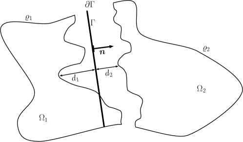
Figure 2: Sketch of the geometry for the reduced Darcy problem (56).

For $i\in\mathopen{}\mathclose{{}\left\{1,2}\right\}$, let $q_{i}\in L^{2}\mathopen{}\mathclose{{}\left(\Omega_{i}}\right)$, $q_{\Gamma}\in L^{2}\mathopen{}\mathclose{{}\left(\Gamma}\right)$, and $d_{1},d_{2}\in W^{1,\infty}\mathopen{}\mathclose{{}\left(\Gamma}\right)$ with $d:=d_{1}+d_{2}>d_{\mathrm{min}}$ for a constant $d_{\mathrm{min}}>0$. Besides, let $\mathbf{K}_{i}\in L^{\infty}\mathopen{}\mathclose{{}\left(\Omega_{i};\mathbb{R}^{n\times n}}\right)$ for $i\in\mathopen{}\mathclose{{}\left\{1,2}\right\}$ and $\mathbf{K}_{\Gamma}\in L^{\infty}\mathopen{}\mathclose{{}\left(\Gamma;\mathbb{R}^{n\times n}}\right)$ as well as $\smash{K_{\Gamma}^{\perp}\in L^{\infty}\mathopen{}\mathclose{{}\left(\Gamma}\right)}$. In addition, let $\mathbf{K}_{1}$, $\mathbf{K}_{2}$, and $\mathbf{K}_{\Gamma}$ be symmetric and uniformly elliptic, i.e., there exist constants $\kappa_{\mathrm{max}}^{\mathrm{b}}\geq\kappa_{\mathrm{min}}^{\mathrm{b}}>0$ and $\kappa_{\mathrm{max}}^{\Gamma}\geq\kappa_{\mathrm{min}}^{\Gamma}>0$ such that

(53a) $$\kappa_{\mathrm{min}}^{\mathrm{b}}{\mathopen{}\mathclose{{}\left|{\bm{z}}}\right|}_{2}^{2} \leq\mathbf{K}_{i}\mathopen{}\mathclose{{}\left({\bm{x}}_{i}}\right){\bm{z}}\cdot{\bm{z}}\leq\kappa_{\mathrm{max}}^{\mathrm{b}}{\mathopen{}\mathclose{{}\left|{\bm{z}}}\right|}_{2}^{2},$$

(53b) $$\kappa_{\mathrm{min}}^{\Gamma}{\mathopen{}\mathclose{{}\left|{\bm{z}}}\right|}_{2}^{2} \leq\,\mathbf{K}_{\Gamma}\mathopen{}\mathclose{{}\left({\bm{t}}}\right){\bm{z}}\cdot{\bm{z}}\,\leq\kappa_{\mathrm{max}}^{\Gamma}{\mathopen{}\mathclose{{}\left|{\bm{z}}}\right|}_{2}^{2}$$

for all $${\bm{z}}\in\mathbb{R}^{n}$$. Besides, we require that

(53c) $$\kappa_{\mathrm{min}}^{\Gamma} \leq K_{\Gamma}^{\perp}\mathopen{}\mathclose{{}\left({\bm{t}}}\right)\leq\kappa_{\mathrm{max}}^{\Gamma}.$$

The conditions in Eq. 53 are supposed to hold for almost every ${\bm{x}}_{i}\in\Omega_{i}$, $i\in\mathopen{}\mathclose{{}\left\{1,2}\right\}$, and $\smash{(0,{\bm{t}}^{T})^{T}_{\mathcal{N}}}\in\Gamma$. Moreover, let $\xi>\frac{1}{2}$ and $\beta_{\Gamma}\in L^{\infty}(\Gamma)$ be defined as in Eq. 50.

Further, we define the solution and test function spaces

(54) $$\Phi_{\mathrm{b}} :=\bigtimes\nolimits_{i=1,2}H^{1}_{0,\varrho_{i}}\mathopen{}\mathclose{{}\left(\Omega_{i}}\right),\quad\enspace\Phi_{\Gamma}:=H^{1}_{0}\mathopen{}\mathclose{{}\left(\Gamma}\right),\quad\enspace\Phi:=\Phi_{\mathrm{b}}\times\Phi_{\Gamma}.$$

The space $\Phi$ is equipped with the norm ${\mathopen{}\mathclose{{}\left\|\cdot}\right\|}_{\Phi}$ defined by

(55) $${\mathopen{}\mathclose{{}\left\|\varphi}\right\|}_{\Phi}^{2}:={\mathopen{}\mathclose{{}\left\|\varphi_{\mathrm{b}}}\right\|}_{\Phi_{\mathrm{b}}}^{2}+{\mathopen{}\mathclose{{}\left\|\varphi_{\Gamma}}\right\|}_{\Phi_{\Gamma}}^{2}:=\mathopen{}\mathclose{{}\left({\mathopen{}\mathclose{{}\left\|\varphi_{1}}\right\|}^{2}_{H^{1}\mathopen{}\mathclose{{}\left(\Omega_{1}}\right)}+{\mathopen{}\mathclose{{}\left\|\varphi_{2}}\right\|}^{2}_{H^{1}\mathopen{}\mathclose{{}\left(\Omega_{2}}\right)}}\right)+{\mathopen{}\mathclose{{}\left\|\varphi_{\Gamma}}\right\|}^{2}_{H^{1}\mathopen{}\mathclose{{}\left(\Gamma}\right)}$$

for $\varphi=\mathopen{}\mathclose{{}\left(\varphi_{\mathrm{b}},\varphi_{\Gamma}}\right)\in\Phi$ with $\varphi_{\mathrm{b}}=\mathopen{}\mathclose{{}\left(\varphi_{1},\varphi_{2}}\right)\in\Phi_{\mathrm{b}}$. Then, a weak formulation of the reduced interface model derived in Section 3 is given by the following problem. Find $p=\mathopen{}\mathclose{{}\left(p_{\mathrm{b}},p_{\Gamma}}\right)\in\Phi$ such that

(56) $$\mathcal{A}\mathopen{}\mathclose{{}\left(p,\varphi}\right) =\mathcal{R}\mathopen{}\mathclose{{}\left(\varphi}\right)\qquad\text{for all }\varphi=\mathopen{}\mathclose{{}\left(\varphi_{\mathrm{b}},\varphi_{\Gamma}}\right)\in\Phi.$$

Here, for $p=\mathopen{}\mathclose{{}\left(p_{\mathrm{b}},p_{\Gamma}}\right),\varphi=\mathopen{}\mathclose{{}\left(\varphi_{\mathrm{b}},\varphi_{\Gamma}}\right)\in\Phi$ with $p_{\mathrm{b}}=\mathopen{}\mathclose{{}\left(p_{1},p_{2}}\right),\varphi_{\mathrm{b}}=\mathopen{}\mathclose{{}\left(\varphi_{1},\varphi_{2}}\right)\in\Phi_{\mathrm{b}}$, the bilinear form $\mathcal{A}\colon\Phi\times\Phi\rightarrow\mathbb{R}$ and the linear form $\mathcal{R}\colon\Phi\rightarrow\mathbb{R}$ are defined by

(57a) $$\mathcal{A}\mathopen{}\mathclose{{}\left(p,\varphi}\right) :=\mathcal{A}_{\mathrm{b}}\mathopen{}\mathclose{{}\left(p_{\mathrm{b}},\varphi_{\mathrm{b}}}\right)+\mathcal{A}_{\Gamma}\mathopen{}\mathclose{{}\left(p,\varphi_{\Gamma}}\right)+\mathcal{I}\mathopen{}\mathclose{{}\left(p,\varphi}\right),$$

(57b) $$\mathcal{R}\mathopen{}\mathclose{{}\left(\varphi}\right) :=\mathcal{R}_{\mathrm{b}}\mathopen{}\mathclose{{}\left(\varphi_{\mathrm{b}}}\right)+\mathcal{R}_{\Gamma}\mathopen{}\mathclose{{}\left(\varphi_{\Gamma}}\right).$$

Specifically, the bilinear forms $\mathcal{A}_{\mathrm{b}}\colon\Phi_{\mathrm{b}}\times\Phi_{\mathrm{b}}\rightarrow\mathbb{R}$, $\mathcal{A}_{\Gamma}\colon\Phi\times\Phi_{\Gamma}\rightarrow\mathbb{R}$, and $\mathcal{I}\colon\Phi\times\Phi\rightarrow\mathbb{R}$, which in this order represent the flow in the bulk domain, the effective flow inside the fracture, and the interfacial coupling between them, as well as the corresponding linear forms $\mathcal{R}_{\mathrm{b}}\colon\Phi_{\mathrm{b}}\rightarrow\mathbb{R}$ and $\mathcal{R}_{\Gamma}\colon\Phi_{\Gamma}\rightarrow\mathbb{R}$, are given by

(58a) $$\mathcal{A}_{\mathrm{b}}\mathopen{}\mathclose{{}\left(p_{\mathrm{b}},\varphi_{\mathrm{b}}}\right) :=\sum_{i=1,2}\int_{\Omega_{i}}\mathbf{K}_{i}\nabla p_{i}\cdot\nabla\varphi_{i}\,\mathrm{d}V,$$

(58b) $$\mathcal{A}_{\Gamma}\mathopen{}\mathclose{{}\left(p,\varphi_{\Gamma}}\right) :=\!\int_{\Gamma}\mathbf{K}_{\Gamma}\nabla\varphi_{\Gamma}\cdot\!\mathopen{}\mathclose{{}\left[\nabla\mathopen{}\mathclose{{}\left(dp_{\Gamma}}\right)-{\mathopen{}\mathclose{{}\left.\kern-1.2ptp_{1}\vphantom{\big{|}}}\right|_{\Gamma_{1}}}\!\nabla d_{1}-{\mathopen{}\mathclose{{}\left.\kern-1.2ptp_{2}\vphantom{\big{|}}}\right|_{\Gamma_{2}}}\!\nabla d_{2}}\right]\,\mathrm{d}\sigma,$$

(58c) $$\begin{split}\mathcal{I}\mathopen{}\mathclose{{}\left(p,\varphi}\right)&:=\int_{\Gamma}\frac{K_{\Gamma}^{\perp}}{d}\llbracket p_{\mathrm{b}}\rrbracket\llbracket\varphi_{\mathrm{b}}\rrbracket\,\mathrm{d}\sigma+\int_{\Gamma}\beta_{\Gamma}\big{(}p_{\Gamma}-\{\mskip-5.0mu\{p_{\mathrm{b}}\}\mskip-5.0mu\}\big{)}\big{(}\varphi_{\Gamma}-\{\mskip-5.0mu\{\varphi_{\mathrm{b}}\}\mskip-5.0mu\}\big{)}\,\mathrm{d}\sigma,\end{split}$$

(58d) $$\mathcal{R}_{\mathrm{b}}\mathopen{}\mathclose{{}\left(\varphi_{\mathrm{b}}}\right) :=\sum_{i=1,2}\int_{\Omega_{i}}q_{i}\varphi_{i}\,\mathrm{d}V,$$

(58e) $$\mathcal{R}_{\Gamma}\mathopen{}\mathclose{{}\left(\varphi_{\Gamma}}\right) :=\int_{\Gamma}q_{\Gamma}\varphi_{\Gamma}\,\mathrm{d}\sigma.$$

The wellposedness of the weak problem (56) is guaranteed by the following result.

Theorem 4.1.

Given the condition

(59) $$\mathopen{}\mathclose{{}\left[\frac{\kappa_{\mathrm{max}}^{\Gamma}}{\kappa_{\mathrm{min}}^{\Gamma}}}\right]^{2}\frac{D}{d_{\mathrm{min}}}\bigg{[}(2\xi-1){\mathopen{}\mathclose{{}\left\|\nabla d}\right\|}_{L^{\infty}\mathopen{}\mathclose{{}\left(\Gamma;\,\mathbb{R}^{n}}\right)}^{2}+{\mathopen{}\mathclose{{}\left\|\nabla d_{1}-\nabla d_{2}}\right\|}_{L^{\infty}\mathopen{}\mathclose{{}\left(\Gamma;\,\mathbb{R}^{n}}\right)}^{2}\bigg{]}<16,$$

the reduced Darcy problem (56) has a unique solution $\mathopen{}\mathclose{{}\left(p_{\mathrm{b}},p_{\Gamma}}\right)\in\Phi$.

We remark that the condition in Eq. 59 appears reasonable as it prohibits large permeability fluctuations within the fracture and rules out fractures that are geometrically extreme in terms of steep aperture gradients and large aperture fluctuations.

Proof 4.2.

The proof is based on the Lax-Milgram theorem. It is easy to see that the bilinear form $\mathcal{A}$ from Eq. 57a is continuous with respect to the norm in Eq. 55. In the following, we will show that $\mathcal{A}$ is coercive under the condition in Eq. 59.

Using (53a) and Poincaré’s inequality, it is evident that the bilinear form $\mathcal{A}_{\mathrm{b}}$ is coercive on $\Phi_{\mathrm{b}}$. Further, concerning the bilinear form $\mathcal{A}_{\Gamma}$, a simple calculation yields

(60) $$\begin{split}&\big{[}\varphi_{\Gamma}-{\mathopen{}\mathclose{{}\left.\kern-1.2pt\varphi_{1}\vphantom{\big{|}}}\right|_{\Gamma_{1}}}\big{]}\nabla d_{1}+\big{[}\varphi_{\Gamma}-{\mathopen{}\mathclose{{}\left.\kern-1.2pt\varphi_{2}\vphantom{\big{|}}}\right|_{\Gamma_{2}}}\big{]}\nabla d_{2}\\ &\hskip 99.58464pt=\big{(}\varphi_{\Gamma}-\{\mskip-5.0mu\{\varphi_{\mathrm{b}}\}\mskip-5.0mu\}\big{)}\nabla d+\frac{1}{2}\llbracket\varphi_{\mathrm{b}}\rrbracket\big{(}\nabla d_{1}-\nabla d_{2}\big{)}.\end{split}$$

Thus, using the condition (53) and Hölder’s inequality, we have

(61) $$\begin{split}\mathcal{A}_{\Gamma}\mathopen{}\mathclose{{}\left(\varphi,\varphi_{\Gamma}}\right)&=\int_{\Gamma}d\mathbf{K}_{\Gamma}\nabla\varphi_{\Gamma}\cdot\nabla\varphi_{\Gamma}\,\mathrm{d}\sigma+\smash{\sum_{i=1,2}}\smash{\int_{\Gamma}}\big{[}\varphi_{\Gamma}-{\mathopen{}\mathclose{{}\left.\kern-1.2pt\varphi_{i}\vphantom{\big{|}}}\right|_{\Gamma_{i}}}\big{]}\mathbf{K}_{\Gamma}\nabla\varphi_{\Gamma}\cdot\nabla d_{i}\,\mathrm{d}\sigma\\[6.0pt] &\geq\kappa_{\mathrm{min}}^{\Gamma}d_{\mathrm{min}}{\mathopen{}\mathclose{{}\left\|\nabla\varphi_{\Gamma}}\right\|}_{L^{2}\mathopen{}\mathclose{{}\left(\Gamma;\,\mathbb{R}^{n}}\right)}^{2}\\ &\quad-\kappa_{\mathrm{max}}^{\Gamma}{\mathopen{}\mathclose{{}\left\|\nabla d}\right\|}_{L^{\infty}\mathopen{}\mathclose{{}\left(\Gamma;\,\mathbb{R}^{n}}\right)}{\mathopen{}\mathclose{{}\left\|\varphi_{\Gamma}-\{\mskip-5.0mu\{\varphi_{\mathrm{b}}\}\mskip-5.0mu\}}\right\|}_{L^{2}\mathopen{}\mathclose{{}\left(\Gamma}\right)}{\mathopen{}\mathclose{{}\left\|\nabla\varphi_{\Gamma}}\right\|}_{L^{2}\mathopen{}\mathclose{{}\left(\Gamma;\,\mathbb{R}^{n}}\right)}\\ &\quad-\frac{\kappa_{\mathrm{max}}^{\Gamma}}{2}{\mathopen{}\mathclose{{}\left\|\nabla d_{1}-\nabla d_{2}}\right\|}_{L^{\infty}\mathopen{}\mathclose{{}\left(\Gamma;\,\mathbb{R}^{n}}\right)}{\mathopen{}\mathclose{{}\left\|\llbracket\varphi_{\mathrm{b}}\rrbracket}\right\|}_{L^{2}\mathopen{}\mathclose{{}\left(\Gamma}\right)}{\mathopen{}\mathclose{{}\left\|\nabla\varphi_{\Gamma}}\right\|}_{L^{2}\mathopen{}\mathclose{{}\left(\Gamma;\,\mathbb{R}^{n}}\right)}.\end{split}$$

By Young’s inequality, for any $\delta,\varepsilon>0$, it holds

$${\mathopen{}\mathclose{{}\left\|\varphi_{\Gamma}-\{\mskip-5.0mu\{\varphi_{\mathrm{b}}\}\mskip-5.0mu\}}\right\|}_{L^{2}\mathopen{}\mathclose{{}\left(\Gamma}\right)}{\mathopen{}\mathclose{{}\left\|\nabla\varphi_{\Gamma}}\right\|}_{L^{2}\mathopen{}\mathclose{{}\left(\Gamma;\,\mathbb{R}^{n}}\right)} \leq\varepsilon{\mathopen{}\mathclose{{}\left\|\varphi_{\Gamma}-\{\mskip-5.0mu\{\varphi_{\mathrm{b}}\}\mskip-5.0mu\}}\right\|}^{2}_{L^{2}\mathopen{}\mathclose{{}\left(\Gamma}\right)}+\frac{1}{4\varepsilon}{\mathopen{}\mathclose{{}\left\|\nabla\varphi_{\Gamma}}\right\|}_{L^{2}\mathopen{}\mathclose{{}\left(\Gamma;\,\mathbb{R}^{n}}\right)}^{2},$$

(62) $${\mathopen{}\mathclose{{}\left\|\llbracket\varphi_{\mathrm{b}}\rrbracket}\right\|}_{L^{2}\mathopen{}\mathclose{{}\left(\Gamma}\right)}{\mathopen{}\mathclose{{}\left\|\nabla\varphi_{\Gamma}}\right\|}_{L^{2}\mathopen{}\mathclose{{}\left(\Gamma;\,\mathbb{R}^{n}}\right)} \leq\delta{\mathopen{}\mathclose{{}\left\|\llbracket\varphi_{\mathrm{b}}\rrbracket}\right\|}_{L^{2}\mathopen{}\mathclose{{}\left(\Gamma}\right)}^{2}+\frac{1}{4\delta}{\mathopen{}\mathclose{{}\left\|\nabla\varphi_{\Gamma}}\right\|}_{L^{2}\mathopen{}\mathclose{{}\left(\Gamma;\,\mathbb{R}^{n}}\right)}^{2}.$$

Besides, with Eq. 53, we have

(63) $$\mathcal{I}\mathopen{}\mathclose{{}\left(\varphi,\varphi}\right)\overset{\eqref{eq:lambda_ineq}}{\geq}\frac{\kappa_{\mathrm{min}}^{\Gamma}}{D}{\mathopen{}\mathclose{{}\left\|\llbracket\varphi_{\mathrm{b}}\rrbracket}\right\|}_{L^{2}\mathopen{}\mathclose{{}\left(\Gamma}\right)}^{2}+\frac{4}{2\xi-1}\frac{\kappa_{\mathrm{min}}^{\Gamma}}{D}{\mathopen{}\mathclose{{}\left\|\varphi_{\Gamma}-\{\mskip-5.0mu\{\varphi_{\mathrm{b}}\}\mskip-5.0mu\}}\right\|}_{L^{2}\mathopen{}\mathclose{{}\left(\Gamma}\right)}^{2}$$

for the bilinear form $\mathcal{I}$. As a consequence, we obtain

(64) $$\begin{split}&\mathcal{B}_{\Gamma}\mathopen{}\mathclose{{}\left(\varphi,\varphi_{\Gamma}}\right)+\mathcal{I}\mathopen{}\mathclose{{}\left(\varphi,\varphi}\right)\\ &\hskip 64.01869pt\geq{\mathopen{}\mathclose{{}\left\|\nabla\varphi_{\Gamma}}\right\|}^{2}_{L^{2}\mathopen{}\mathclose{{}\left(\Gamma;\,\mathbb{R}^{n}}\right)}T_{1}+{\mathopen{}\mathclose{{}\left\|\llbracket\varphi_{\mathrm{b}}\rrbracket}\right\|}_{L^{2}\mathopen{}\mathclose{{}\left(\Gamma}\right)}^{2}T_{2}+{\mathopen{}\mathclose{{}\left\|\varphi_{\Gamma}-\{\mskip-5.0mu\{\varphi_{\mathrm{b}}\}\mskip-5.0mu\}}\right\|}_{L^{2}\mathopen{}\mathclose{{}\left(\Gamma}\right)}^{2}T_{3}\end{split}$$

with $T_{1}$, $T_{2}$, and $T_{3}$ defined by

(65a) $$T_{1} :=\kappa_{\mathrm{min}}^{\Gamma}d_{\mathrm{min}}-\frac{\kappa_{\mathrm{max}}^{\Gamma}}{4\varepsilon}{\mathopen{}\mathclose{{}\left\|\nabla d}\right\|}_{L^{\infty}\mathopen{}\mathclose{{}\left(\Gamma;\,\mathbb{R}^{n}}\right)}-\frac{\kappa_{\mathrm{max}}^{\Gamma}}{8\delta}{\mathopen{}\mathclose{{}\left\|\nabla d_{1}-\nabla d_{2}}\right\|}_{L^{\infty}\mathopen{}\mathclose{{}\left(\Gamma;\,\mathbb{R}^{n}}\right)},$$

(65b) $$T_{2} :=\frac{\kappa_{\mathrm{min}}^{\Gamma}}{D}-\frac{\delta\kappa_{\mathrm{max}}^{\Gamma}}{2}{\mathopen{}\mathclose{{}\left\|\nabla d_{1}-\nabla d_{2}}\right\|}_{L^{\infty}\mathopen{}\mathclose{{}\left(\Gamma;\,\mathbb{R}^{n}}\right)},$$

(65c) $$T_{3} :=\frac{4}{2\xi-1}\frac{\kappa_{\mathrm{min}}^{\Gamma}}{D}-\varepsilon\kappa_{\mathrm{max}}^{\Gamma}{\mathopen{}\mathclose{{}\left\|\nabla d}\right\|}_{L^{\infty}\mathopen{}\mathclose{{}\left(\Gamma;\,\mathbb{R}^{n}}\right)}.$$

Now, w.l.o.g., we assume ${\mathopen{}\mathclose{{}\left\|\nabla d}\right\|}_{L^{\infty}\mathopen{}\mathclose{{}\left(\Gamma;\,\mathbb{R}^{n}}\right)},{\mathopen{}\mathclose{{}\left\|\nabla d_{1}-\nabla d_{2}}\right\|}_{L^{\infty}\mathopen{}\mathclose{{}\left(\Gamma;\,\mathbb{R}^{n}}\right)}\not=0$. Moreover, we choose $\delta,\varepsilon>0$ such that $T_{2}=0$ and $T_{3}=0$, i.e.,

(66) $$\delta =\frac{2\kappa_{\mathrm{min}}^{\Gamma}}{D\kappa_{\mathrm{max}}^{\Gamma}{\mathopen{}\mathclose{{}\left\|\nabla d_{1}-\nabla d_{2}}\right\|}_{L^{\infty}\mathopen{}\mathclose{{}\left(\Gamma;\,\mathbb{R}^{n}}\right)}},\quad\enspace\varepsilon=\frac{4}{2\xi-1}\frac{\kappa_{\mathrm{min}}^{\Gamma}}{D\kappa_{\mathrm{max}}^{\Gamma}{\mathopen{}\mathclose{{}\left\|\nabla d}\right\|}_{L^{\infty}\mathopen{}\mathclose{{}\left(\Gamma;\,\mathbb{R}^{n}}\right)}}.$$

Then, the condition in Eq. 59 guarantees $T_{1}>0$. Thus, by using Poincaré’s inequality, we obtain the coercivity of the overall bilinear form $\mathcal{A}$.

In case of a classical solution, a corresponding strong formulation of the weak system Eq. 56 is, for $i\in\{1,2\}$, given by

(67a) $$-\nabla\cdot\mathopen{}\mathclose{{}\left(\mathbf{K}_{i}\nabla p_{i}}\right) =q_{i}\quad\enspace \text{in }\Omega_{i},$$

(67b) $$-\nabla\cdot\Big{[}\mathbf{K}_{\Gamma}\Big{(}\nabla\mathopen{}\mathclose{{}\left(dp_{\Gamma}}\right)-{\mathopen{}\mathclose{{}\left.\kern-1.2ptp_{1}\vphantom{\big{|}}}\right|_{\Gamma_{1}}}\!\nabla d_{1}-{\mathopen{}\mathclose{{}\left.\kern-1.2ptp_{2}\vphantom{\big{|}}}\right|_{\Gamma_{2}}}\!\nabla d_{2}\Big{)}\Big{]} =q_{\Gamma}-\llbracket\mathbf{K}\nabla p\rrbracket\quad\enspace \text{in }\Gamma,$$

(67c) $$\{\mskip-5.0mu\{\mathbf{K}\nabla p\}\mskip-5.0mu\} =\frac{K_{\Gamma}^{\perp}}{d}\llbracket p\rrbracket\quad\enspace \text{on }\Gamma,$$

(67d) $$\llbracket\mathbf{K}\nabla p\rrbracket =\beta_{\Gamma}\big{(}p_{\Gamma}-\{\mskip-5.0mu\{p\}\mskip-5.0mu\}\big{)}\quad \text{on }\Gamma,$$

(67e) $$p_{i} =0\quad\enspace \text{on }\varrho_{i},$$

(67f) $$p_{\Gamma} =0\qquad \text{on }\partial\Gamma.$$

Here, we observe that the quantity

(68) $${\bm{u}}_{\Gamma}:=-\mathbf{K}_{\Gamma}\Big{(}\nabla\mathopen{}\mathclose{{}\left(dp_{\Gamma}}\right)-{\mathopen{}\mathclose{{}\left.\kern-1.2ptp_{1}\vphantom{\big{|}}}\right|_{\Gamma_{1}}}\!\nabla d_{1}-{\mathopen{}\mathclose{{}\left.\kern-1.2ptp_{2}\vphantom{\big{|}}}\right|_{\Gamma_{2}}}\!\nabla d_{2}\Big{)}$$

in Eq. 67b takes the role of the effective velocity inside the reduced fracture $\Gamma$. Further, for a symmetric fracture with constant aperture, i.e., $d_{1}=d_{2}=d/2\equiv\mathrm{const}.$, the model in Eq. 67 coincides with the model proposed in [22]. Therefore, the new model Eq. 67 can be viewed as an extension of the model in [22] for general asymmetric fractures with spatially varying aperture.

4.1 Model Variants

According to the derivation of the reduced model (67) in Section 3, there should be a gap between the bulk domains $\Omega_{1}$ and $\Omega_{2}$ on either side of the fracture as illustrated in Figure 2. However, for numerical calculations in practice, the bulk domains $\Omega_{1}$ and $\Omega_{2}$ are usually rectified such that the interface $\Gamma$ is part of their boundary, i.e., $\partial\Omega_{1}^{\mathrm{rct.}}\cap\partial\Omega_{2}^{\mathrm{rct.}}=\overline{\Gamma}$. The corresponding reduced model with simplified bulk geometry is obtained from the model in Eq. 67 by replacing the bulk domains $\Omega_{1}$ and $\Omega_{2}$ with the domains

(69a) $$\Omega_{1}^{\mathrm{rct.}}=\big{\{}{\bm{\gamma}}+\lambda{\bm{n}}\in\Omega\ \big{|}\ {\bm{\gamma}}\in\Gamma,\,\lambda<0\big{\}},$$

(69b) $$\Omega_{2}^{\mathrm{rct.}}=\big{\{}{\bm{\gamma}}+\lambda{\bm{n}}\in\Omega\ \big{|}\ {\bm{\gamma}}\in\Gamma,\,\lambda>0\big{\}}.$$

This kind of bulk rectification requires one to neglect the terms containing aperture gradients $\nabla d_{1}$, $\nabla d_{2}$ in the coupling conditions (67c) and (67d). The geometrical difference between the full-dimensional model in Eq. 5, the reduced model in Eq. 67, and the corresponding reduced model with bulk rectification is illustrated in Figure 3.

Figure 3: Bulk domains (a) in the full-dimensional model (5), (b) in the reduced model (67) without rectification, (c) in the reduced model (67) with rectification.

In contrast to the model in [22], the new model Eq. 67 contains aperture gradients $\nabla d_{1}$, $\nabla d_{2}$ in the effective flow equation (67b) and in the coupling conditions (67c) and (67d). In order to study the effect of the aperture gradients as well as the effect of a rectified bulk geometry as discussed above, we define simplified variants of the reduced model (67). On the one hand, we can neglect the aperture gradients $\nabla d_{1}$, $\nabla d_{2}$ in Eq. 67b, i.e., Eq. 67b is replaced by the equation

(70) $$-\nabla\cdot\big{[}\mathbf{K}_{\Gamma}\nabla\mathopen{}\mathclose{{}\left(dp_{\Gamma}}\right)\big{]} =q_{\Gamma}-\llbracket\mathbf{K}\nabla p\rrbracket\quad\enspace \text{in }\Gamma.$$

On the other hand, the aperture gradients $\nabla d_{1}$, $\nabla d_{2}$ could be neglected in the coupling conditions (67c) and (67d), which corresponds to a rectification of the bulk domains $\Omega_{1}$ and $\Omega_{2}$. This suggests to define the following model variants.
     Model I: The new model (67) without change.      Model I-R: The model (67) with the bulk domains $\Omega_{1}$ and $\Omega_{2}$ replaced by the rectified domains $\Omega_{1}^{\mathrm{rct.}}$ and $\Omega_{2}^{\mathrm{rct.}}$ from Eq. 69. Terms containing $\nabla d_{1}$, $\nabla d_{2}$ are neglected in Eqs. 67c and 67d but not in Eq. 67b.      Model II: The model (67) with unchanged bulk domains. Terms containing $\nabla d_{1}$, $\nabla d_{2}$ are neglected in Eq. 67b but not in Eq. 67c and (67d).      Model II-R: The model (67) with the bulk domains $\Omega_{1}$ and $\Omega_{2}$ replaced by the rectified domains $\Omega_{1}^{\mathrm{rct.}}$ and $\Omega_{2}^{\mathrm{rct.}}$ from Eq. 69. Terms containing $\nabla d_{1}$, $\nabla d_{2}$ are neglected completely.
Model II-R is basically the model proposed in [22] with the only difference that the aperture $d$ in Eq. 70 can still be a function that is not necessarily constant as assumed in [22]. In particular, in model II-R, there is no information about the aperture gradients $\nabla d_{1}$, $\nabla d_{2}$ and the bulk geometry at the fracture. In contrast, the new model I includes all this information. The models I-R and II are intermediate models.

5 Discontinuous Galerkin Discretization

In this section, following [4], we formulate three discontinuous Galerkin (DG) discretizations, one for the full-dimensional model (5), one for the reduced models II and II-R, and one for the reduced models I and I-R from Section 4, where, in this order, each discretization extends the previous one. The choice of a DG scheme as discretization for the reduced fracture models comes naturally as it can easily deal with discontinuities across the fracture and suits the formulation of the coupling conditions (67c) and (67d) in terms of jump and average operators. For simplicity, we assume that $\Omega$ is a polytopial domain. Besides, we consider inhomogeneous Dirichlet boundary conditions for all discretizations.

5.1 Meshes and Notations

Let $\mathcal{I}$ be the index family of bulk domains, i.e., $\mathcal{I}=\{1,2,\mathrm{f}\}$ in the full-dimensional case and $\mathcal{I}=\{1,2\}$ for the reduced models. Further, for $i\in\mathcal{I}$, let $\mathcal{T}_{h,i}$ be a polytopial mesh of the bulk domain $\Omega_{i}$ of closed elements $T_{h,i}\in\mathcal{T}_{h,i}$ with disjoint interiors. Besides, we write $\mathcal{T}_{h}:=\bigcup_{i\in\mathcal{I}}\mathcal{T}_{h,i}$ for the overall bulk mesh, which may be non-conforming. Moreover, we denote by $\mathcal{F}_{h}$ the facet grid induced by $\mathcal{T}_{h}$ which contains all one-codimensional intersections between grid elements $T\in\mathcal{T}_{h}$ with neighboring grid elements or the domain boundary $\partial\Omega$. For the reduced models, we denote by $\mathcal{F}^{\Gamma}_{h}$ a one-codimensional polytopial mesh of the interface $\Gamma$ induced by the bulk grids $\mathcal{T}_{h,1}$ and $\mathcal{T}_{h,2}$. Specifically, for the reduced models I-R and II-R, i.e., in case of a reduced model with rectified bulk domains as defined in Eq. 69, the fracture mesh $\mathcal{F}^{\Gamma}_{h}$ is part of the facet grid $\mathcal{F}_{h}$ and given by

(71a) $$\mathcal{F}^{\Gamma}_{h}:=\mathopen{}\mathclose{{}\left\{F\in\mathcal{F}_{h}\ \middle|\ F\subset\overline{\Gamma}}\right\}.$$

In the other case, for the reduced models I and II without bulk rectification, the fracture mesh $$\mathcal{F}_{h}^{\Gamma}$$ can be defined by

(71b) $$\mathcal{F}^{\Gamma}_{h}:=\Big{\{}\mathscr{P}_{\Gamma}(F_{1})\cap\mathscr{P}_{\Gamma}(F_{2})\ \Big{|}\ F_{i}=\partial T_{i}\cap\overline{\Gamma}_{i}\not=\emptyset,\ T_{i}\in\mathcal{T}_{h,i}\ \text{ for }i\in\{1,2\}\Big{\}}.$$

In Eq. 71b, $\mathscr{P}_{\Gamma}$ denotes the orthogonal projection onto the hyperplane $\Gamma$ given by

(72) $$\mathscr{P}_{\Gamma}\colon\Omega\rightarrow\Omega,\enspace\big{(}\eta,{\bm{t}}^{T}\big{)}^{\!T}_{\!\mathcal{N}}\mapsto\big{(}0,{\bm{t}}^{T}\big{)}^{\!T}_{\!\mathcal{N}}.$$

Regarding the facet grid $\mathcal{F}_{h}$, we distinguish between the set of facets $\mathcal{F}_{h}^{\partial}$ on the domain boundary $\partial\Omega$ and the set of facets $\mathcal{F}_{h}^{\circ}$ in the interior of $\Omega$ excluding the interface grid $\mathcal{F}^{\Gamma}_{h}$, i.e., we can write $\mathcal{F}_{h}$ as the disjoint union $\mathcal{F}_{h}=\mathcal{F}_{h}^{\circ}\;\dot{\cup}\;\mathcal{F}_{h}^{\partial}\;\dot{\cup}\;\mathopen{}\mathclose{{}\left(\mathcal{F}^{\Gamma}_{h}\cap\mathcal{F}_{h}}\right)$. In addition, for the reduced models, we denote by $\mathcal{E}_{h}^{\Gamma}$ the set of edges of the interface grid $\mathcal{F}^{\Gamma}_{h}$, i.e., the set of two-codimensional intersections between elements $F\in\mathcal{F}^{\Gamma}_{h}$ or the boundary $\partial\Gamma$. More specifically, we distinguish between the set of edges $\mathcal{E}^{\circ}_{h}$ in the interior of the interface $\Gamma$ and the set of edges $\mathcal{E}^{\partial}_{h}$ at the boundary $\partial\Gamma$ such that $\mathcal{E}^{\Gamma}_{h}=\mathcal{E}^{\circ}_{h}\;\dot{\cup}\;\mathcal{E}^{\partial}_{h}$.

For $A\subset\mathbb{R}^{n}$, let $\mathcal{P}_{k}(A)$ denote the space of polynomials on $A$ whose degrees do not exceed $k\in\mathbb{N}_{0}$. Then, we define the finite-dimensional function spaces

(73a) $$\Phi^{\mathrm{b}}_{h} :=\big{\{}\varphi_{h}\in L^{2}(\Omega)\ \big{|}\ {\mathopen{}\mathclose{{}\left.\kern-1.2pt\varphi_{h}\vphantom{\big{|}}}\right|_{T}}\in\mathcal{P}_{k_{T}}(T)\ \text{for all}\ T\in\mathcal{T}_{h}\big{\}},$$

(73b) $$\Phi^{\Gamma}_{h} :=\big{\{}\varphi^{\Gamma}_{h}\in L^{2}(\Gamma)\ \big{|}\ {\mathopen{}\mathclose{{}\left.\kern-1.2pt\varphi^{\Gamma}_{h}\vphantom{\big{|}}}\right|_{F}}\in\mathcal{P}_{k_{F}}(F)\ \text{for all}\ F\in\mathcal{F}_{h}^{\Gamma}\big{\}},$$

(73c) $$\Phi_{h} :=\Phi_{h}^{\mathrm{b}}\times\Phi_{h}^{\Gamma}$$

with individual polynomial degrees $k_{T}\in\mathbb{N}$ and $k_{F}\in\mathbb{N}$ for each bulk element $T\in\mathcal{T}_{h}$ and interface element $F\in\mathcal{F}_{h}^{\Gamma}$. Further, we introduce jump and average operators for DG discretizations. Although we use the same notation, we note that the following definition is different from Definition 3.3.

Definition 5.1 (Jump and average operators for DG schemes).

Let $\mathcal{M}_{h}=\mathcal{T}_{h}$ and $\mathcal{S}_{h}^{\circ}=\mathcal{F}_{h}^{\circ}$, or $\mathcal{M}_{h}=\mathcal{F}_{h}^{\Gamma}$ and $\mathcal{S}_{h}^{\circ}=\mathcal{E}_{h}^{\circ}$. Further, we define the function spaces

(74) $$\Sigma(\mathcal{M}_{h}):=\prod_{M\in\mathcal{M}_{h}}\!L^{2}(\partial M),\qquad L^{2}(\mathcal{S}_{h}^{\circ}):=\prod_{S\in\mathcal{S}_{h}^{\circ}}L^{2}(S).$$

In general, functions in $\Sigma(\mathcal{M}_{h})$ will be double-valued on facets $S\in\mathcal{S}_{h}^{\circ}$. For a function $\varphi_{h}\in\Sigma(\mathcal{M}_{h})$, we denote the component of $\varphi_{h}$ associated with the mesh element $M\in\mathcal{M}_{h}$ by $\varphi_{h}^{M}$. Besides, for a mesh element $M\in\mathcal{M}_{h}$, we write ${\bm{n}}_{M}$ for the outer unit normal on $\partial M$. We can now define the jump and average operators

(75a) $$\llbracket\,\cdot\,\rrbracket \colon\Sigma(\mathcal{M}_{h})\rightarrow\mathopen{}\mathclose{{}\left[L^{2}(\mathcal{S}_{h}^{\circ})}\right]^{n}, \qquad\ \;\llbracket\,\cdot\,\rrbracket \colon\big{[}\Sigma(\mathcal{M}_{h})\big{]}^{n}\rightarrow L^{2}(\mathcal{S}_{h}^{\circ}),$$

(75b) $$\{\mskip-5.0mu\{\,\cdot\,\}\mskip-5.0mu\} \colon\Sigma(\mathcal{M}_{h})\rightarrow L^{2}(\mathcal{S}_{h}^{\circ}), \qquad\{\mskip-5.0mu\{\,\cdot\,\}\mskip-5.0mu\} \colon\big{[}\Sigma(\mathcal{M}_{h})\big{]}^{n}\rightarrow\mathopen{}\mathclose{{}\left[L^{2}(\mathcal{S}_{h}^{\circ})}\right]^{n}.$$

Let $\varphi_{h}\in\Sigma(\mathcal{M}_{h})$ and ${\bm{\zeta}}_{h}\in\big{[}\Sigma(\mathcal{M}_{h})\big{]}^{n}$. For an internal facet $S\in\mathcal{S}_{h}^{\circ}$ with adjacent mesh elements $M_{1}\not=M_{2}\in\mathcal{M}_{h}$, we define

(76a) $${\mathopen{}\mathclose{{}\left.\kern-1.2pt\llbracket\varphi_{h}\rrbracket\vphantom{\big{|}}}\right|_{S}} :=\varphi_{h}^{M_{1}}{\bm{n}}_{M_{1}}+\varphi_{h}^{M_{2}}{\bm{n}}_{M_{2}},\qquad \enspace{\mathopen{}\mathclose{{}\left.\kern-1.2pt\llbracket{\bm{\zeta}}_{h}\rrbracket\vphantom{\big{|}}}\right|_{S}} :={\bm{\zeta}}_{h}^{M_{1}}\cdot{\bm{n}}_{M_{1}}+{\bm{\zeta}}_{h}^{M_{2}}\cdot{\bm{n}}_{M_{2}},$$

(76b) $${\mathopen{}\mathclose{{}\left.\kern-1.2pt\{\mskip-5.0mu\{\varphi_{h}\}\mskip-5.0mu\}\vphantom{\big{|}}}\right|_{S}} :=\frac{1}{2}\mathopen{}\mathclose{{}\left(\varphi_{h}^{M_{1}}+\varphi_{h}^{M_{2}}}\right),\qquad {\mathopen{}\mathclose{{}\left.\kern-1.2pt\{\mskip-5.0mu\{{\bm{\zeta}}_{h}\}\mskip-5.0mu\}\vphantom{\big{|}}}\right|_{S}} :=\frac{1}{2}\mathopen{}\mathclose{{}\left({\bm{\zeta}}_{h}^{M_{1}}+{\bm{\zeta}}_{h}^{M_{2}}}\right).$$

5.2 Discrete Model with Full-Dimensional Fracture

Let $g\in H^{1/2}(\partial\Omega)$ denote the given pressure on the boundary $\partial\Omega$ for the Dirichlet condition in Eq. 5b. Then, in order to obtain a DG discretization of the full-dimensional model (5), we define the bilinear form $\mathcal{A}_{h}^{\mathrm{b}}\colon\Phi_{h}^{\mathrm{b}}\times\Phi_{h}^{\mathrm{b}}\rightarrow\mathbb{R}$ associated with bulk flow and the corresponding linear form $\mathcal{R}_{h}^{\mathrm{b}}\colon\Phi^{\mathrm{b}}_{h}\rightarrow\mathbb{R}$ by

(77a) $$\begin{split}\mathcal{A}_{h}^{\mathrm{b}}(p_{h}^{\mathrm{b}},\varphi_{h}^{\mathrm{b}})&=\sum_{T_{\in}\mathcal{T}_{h}}\int_{T}\mathbf{K}\nabla p_{h}^{\mathrm{b}}\cdot\nabla\varphi_{h}^{\mathrm{b}}\,\mathrm{d}V+\sum_{F\in\mathcal{F}_{h}^{\circ}}\int_{F}\mu_{F}\llbracket p_{h}^{\mathrm{b}}\rrbracket\cdot\llbracket\varphi_{h}^{\mathrm{b}}\rrbracket\,\mathrm{d}\sigma\\ &\quad-\sum_{F\in\mathcal{F}_{h}^{\circ}}\int_{F}\Big{[}\llbracket\varphi_{h}^{\mathrm{b}}\rrbracket\cdot\{\mskip-5.0mu\{\mathbf{K}\nabla p_{h}^{\mathrm{b}}\}\mskip-5.0mu\}+\llbracket p_{h}^{\mathrm{b}}\rrbracket\cdot\{\mskip-5.0mu\{\mathbf{K}\nabla\varphi_{h}^{\mathrm{b}}\}\mskip-5.0mu\}\Big{]}\,\mathrm{d}\sigma\\ &\quad+\sum_{F\in\mathcal{F}_{h}^{\partial}}\int_{F}\mu_{F}^{\mathrm{b}}p_{h}^{\mathrm{b}}\varphi_{h}^{\mathrm{b}}\,\mathrm{d}\sigma-\!\sum_{F\in\mathcal{F}_{h}^{\partial}}\int_{F}\big{[}p_{h}^{\mathrm{b}}\mathbf{K}\nabla\varphi_{h}^{\mathrm{b}}+\varphi_{h}^{\mathrm{b}}\mathbf{K}\nabla p_{h}^{\mathrm{b}}\big{]}\!\cdot\mathrm{d}{\bm{\sigma}},\end{split}$$

(77b) $$\begin{split}\mathcal{R}^{\mathrm{b}}_{h}(\varphi_{h}^{\mathrm{b}})&=\sum_{T\in\mathcal{T}_{h}}\int_{T}q\varphi_{h}^{\mathrm{b}}\,\mathrm{d}V+\sum_{F\in\mathcal{F}_{h}^{\partial}}\bigg{[}\int_{F}\mu_{F}^{\mathrm{b}}g\varphi_{h}^{\mathrm{b}}\,\mathrm{d}\sigma-\int_{F}g\mathbf{K}\nabla\varphi_{h}^{\mathrm{b}}\cdot\mathrm{d}{\bm{\sigma}}\bigg{]}.\end{split}$$

In Eq. 77, $\mu_{F}^{\mathrm{b}}$ is a penalty parameter which we define facet-wise, for $F\in\mathcal{F}_{h}\setminus\mathcal{F}_{h}^{\Gamma}$, by

(78) $$\mu_{F}^{\mathrm{b}}:=\begin{cases}\mu_{0}^{\mathrm{b}}\frac{(k_{T}+1)(k_{T}+n)}{h_{T}},&\text{if }F\in\mathcal{F}_{h}^{\partial},\,F\subset\partial T,\,T\in\mathcal{T}_{h},\\ \mu_{0}^{\mathrm{b}}\!\max\limits_{T=T_{1},T_{2}}\!\mathopen{}\mathclose{{}\left\{\!\frac{(k_{T}+1)(k_{T}+n)}{h_{T}}\!}\right\},&\text{if }F\in\mathcal{F}_{h}^{\circ},\,F\subset\partial T_{1}\cap\partial T_{2},\,T_{1}\not=T_{2}\in\mathcal{T}_{h}.\end{cases}$$

In Eq. 78, $\mu_{0}^{\mathrm{b}}>0$ is a sufficiently large constant and $h_{T}$ denotes the maximum edge length of a grid element $T\in\mathcal{T}_{h}$.

A DG discretization of the full-dimensional system (5) is now given by the following problem. Find $p_{h}^{\mathrm{b}}\in\Phi_{h}^{\mathrm{b}}$ such that

(79) $$\mathcal{A}_{h}^{\mathrm{b}}(p_{h}^{\mathrm{b}},\varphi_{h}^{\mathrm{b}})=\mathcal{R}_{h}^{\mathrm{b}}(\varphi_{h}^{\mathrm{b}})\qquad\text{for all }\varphi_{h}^{\mathrm{b}}\in\Phi_{h}^{\mathrm{b}}.$$

5.3 Discrete Model with Interfacial Fracture

Let $g_{\Gamma}\in H^{1/2}(\Gamma)$ and $g=(g_{1},g_{2})\in H^{1/2}(\varrho_{1})\times H^{1/2}(\varrho_{2})$ denote the given pressure functions on the external boundaries for the Dirichlet conditions (67e) and (67f). We continue to extend the DG discretization in Eq. 79 to a discretization of the reduced interface models I, I-R, II, and II-R from Section 4. Here, the models I and I-R and the models II and II-R can be treated together, respectively, since they only differ in their bulk geometry with otherwise identical weak formulation.

We define the bilinear forms $\mathcal{A}_{h}^{\Gamma_{1}}\colon\Phi_{h}^{\Gamma}\times\Phi_{h}^{\Gamma}\rightarrow\mathbb{R}$, $\mathcal{A}_{h}^{\Gamma_{2}}\colon\Phi_{h}^{\mathrm{b}}\times\Phi_{h}^{\Gamma}$, and $\mathcal{I}_{h}\colon\Phi_{h}\times\Phi_{h}\rightarrow\mathbb{R}$, as well as the linear form $\mathcal{R}_{h}^{\Gamma}\colon\Phi_{h}^{\Gamma}\rightarrow\mathbb{R}$, by

(80a) $$\begin{split}\mathcal{A}^{\Gamma_{1}}_{h}(p_{h}^{\Gamma},\varphi_{h}^{\Gamma})&=\sum_{F\in F_{h}^{\Gamma}}\int_{F}\mathbf{K}_{\Gamma}\nabla(dp_{h}^{\Gamma})\cdot\nabla\varphi_{h}^{\Gamma}\,\mathrm{d}\sigma+\sum_{E\in\mathcal{E}^{\circ}_{h}}\int_{E}\mu^{\Gamma}_{E}\llbracket p_{h}^{\Gamma}\rrbracket\cdot\llbracket\varphi_{h}^{\Gamma}\rrbracket\,\mathrm{d}r\\ &\quad-\sum_{E\in\mathcal{E}^{\circ}_{h}}\int_{E}\Big{[}\llbracket\varphi_{h}^{\Gamma}\rrbracket\cdot\{\mskip-5.0mu\{\mathbf{K}_{\Gamma}\nabla(dp_{h}^{\Gamma})\}\mskip-5.0mu\}+\llbracket dp_{h}^{\Gamma}\rrbracket\cdot\{\mskip-5.0mu\{\mathbf{K}_{\Gamma}\nabla\varphi_{h}^{\Gamma}\}\mskip-5.0mu\}\Big{]}\,\mathrm{d}r\\ &\mkern-16.0mu+\sum_{E\in\mathcal{E}_{h}^{\partial}}\bigg{[}\int_{E}\mu^{\Gamma}_{E}p_{h}^{\Gamma}\varphi_{h}^{\Gamma}\,\mathrm{d}r-\int_{E}\Big{[}\varphi_{h}^{\Gamma}\mathbf{K}_{\Gamma}\nabla(dp_{h}^{\Gamma})-dp_{h}^{\Gamma}\mathbf{K}_{\Gamma}\nabla\varphi_{h}^{\Gamma}\Big{]}\cdot\mathrm{d}{\bm{r}}\bigg{]},\end{split}$$

(80b) $$\begin{split}\mathcal{A}^{\Gamma_{2}}_{h}(p_{h}^{\mathrm{b}},\varphi_{h}^{\Gamma})&=-\!\sum_{F\in F_{h}^{\Gamma}}\int_{F}\Big{[}p_{h}^{(1)}\nabla d_{1}+p_{h}^{(2)}\nabla d_{2}\Big{]}\!\cdot\mathbf{K}_{\Gamma}\nabla\varphi_{h}^{\Gamma}\,\mathrm{d}\sigma\\ &\mkern-48.0mu+\!\sum_{E\in\mathcal{E}_{h}^{\circ}}\int_{E}\{\mskip-5.0mu\{p_{h}^{\mathrm{b}}\}\mskip-5.0mu\}\llbracket\varphi_{h}^{\Gamma}\rrbracket\cdot\mathbf{K}_{\Gamma}\nabla d\,\mathrm{d}r+\!\sum_{E\in\mathcal{E}^{\partial}_{h}}\int_{E}\varphi_{h}^{\Gamma}\big{[}p_{h}^{(1)}\nabla d_{1}+p_{h}^{(2)}\nabla d_{2}\big{]}\!\cdot\mathrm{d}{\bm{r}},\end{split}$$

(80c) $$\begin{split}\mathcal{I}_{h}(p_{h},\varphi_{h})&=\sum_{F\in\mathcal{F}_{h}^{\Gamma}}\int_{F}\frac{K_{\Gamma}^{\perp}}{d}\llbracket p_{h}^{\mathrm{b}}\rrbracket\cdot\llbracket\varphi_{h}^{\mathrm{b}}\rrbracket\,\mathrm{d}\sigma\\ &\qquad+\sum_{F\in\mathcal{F}_{h}^{\Gamma}}\int_{F}\beta_{\Gamma}\big{(}p^{\Gamma}_{h}-\{\mskip-5.0mu\{p^{\mathrm{b}}_{h}\}\mskip-5.0mu\}\big{)}\big{(}\varphi^{\Gamma}_{h}-\{\mskip-5.0mu\{\varphi^{\mathrm{b}}_{h}\}\mskip-5.0mu\}\big{)}\,\mathrm{d}\sigma,\end{split}$$

(80d) $$\mathcal{R}^{\Gamma}_{h}(\varphi_{h})= \!\sum_{F\in F_{h}^{\Gamma}}\!\int_{F}q_{\Gamma}\varphi^{\Gamma}_{h}\,\mathrm{d}\sigma+\!\sum_{E\in\mathcal{E}_{h}^{\partial}}\!\bigg{[}\!\int_{E}\mu_{\Gamma}g_{\Gamma}\varphi_{h}^{\Gamma}\,\mathrm{d}r-\!\int_{E}dg_{\Gamma}\mathbf{K}_{\Gamma}\nabla\varphi_{h}^{\Gamma}\cdot\mathrm{d}{\bm{r}}\bigg{]},$$

where $p_{h}=(p_{h}^{\mathrm{b}},p_{h}^{\Gamma}),\varphi_{h}=(\varphi_{h}^{\mathrm{b}},\varphi_{h}^{\Gamma})\in\Phi_{h}$ with $p_{h}^{\mathrm{b}}=\smash{\big{(}p_{h}^{(1)},p_{h}^{(2)}\big{)}}\in\Phi_{h}^{\mathrm{b}}$. For the reduced models I and II without bulk rectification, the evaluation of bulk functions in $\smash{\Phi_{h}^{\mathrm{b}}}$ on the interface $\Gamma$ in the Eqs. 80b and 80c is to be understood in the sense of restrictions to the interfaces $\Gamma_{1}$ and $\Gamma_{2}$ as defined in Eq. 17. Besides, in Eq. 80a, $\smash{\mu^{\Gamma}_{E}}$ is a penalty parameter on the interface $\Gamma$ that is defined in analogy to Eq. 78.

A DG discretization of the the reduced interface models II and II-R is now given by the following problem. Find $p_{h}=(p_{h}^{\mathrm{b}},p_{h}^{\Gamma})\in\Phi_{h}$ such that

(81) $$\mathcal{A}^{\mathrm{b}}_{h}(p_{h}^{\mathrm{b}},\varphi_{h}^{\mathrm{b}})+\mathcal{A}^{\Gamma_{1}}_{h}(p_{h}^{\Gamma},\varphi_{h}^{\Gamma})+\mathcal{I}_{h}(p_{h},\varphi_{h})=\mathcal{R}^{\mathrm{b}}_{h}(\varphi_{h}^{\mathrm{b}})+\mathcal{R}^{\Gamma}_{h}(\varphi_{h}^{\Gamma})$$

holds for all $\varphi_{h}=(\varphi_{h}^{\mathrm{b}},\varphi_{h}^{\Gamma})\in\Phi_{h}$.

Finally, a DG discretization of the reduced models I and I-R extending the discretization in Eq. 81 can be formulated as follows. Find $p_{h}=(p_{h}^{\mathrm{b}},p_{h}^{\Gamma})\in\Phi_{h}$ so that

(82) $$\mathcal{A}^{\mathrm{b}}_{h}(p_{h}^{\mathrm{b}},\varphi_{h}^{\mathrm{b}})+\mathcal{A}^{\Gamma_{1}}_{h}(p_{h}^{\Gamma},\varphi_{h}^{\Gamma})+\mathcal{A}^{\Gamma_{2}}_{h}(p_{h}^{\mathrm{b}},\varphi_{h}^{\Gamma})+\mathcal{I}_{h}(p_{h},\varphi_{h})=\mathcal{R}^{\mathrm{b}}_{h}(\varphi_{h}^{\mathrm{b}})+\mathcal{R}^{\Gamma}_{h}(\varphi_{h}^{\Gamma})$$

holds for all $\varphi_{h}=(\varphi_{h}^{\mathrm{b}},\varphi_{h}^{\Gamma})\in\Phi_{h}$.

6 Numerical Results

We present numerical results to validate the new reduced interface model (67) and explore its capabilities. In particular, we investigate how the use of a simplified bulk geometry and the negligence of aperture gradients $\nabla d_{1}$, $\nabla d_{2}$ affects the accuracy of the reduced model Eq. 67. For this, numerical solutions of the reduced models I, I-R, II, and II-R from Section 4.1 are compared with a numerical reference solution of the full-dimensional model (5). Specifically, for the full-dimensional reference solution, the average pressure $p_{\Gamma}^{\mathrm{ref}}$ across the fracture is computed according to Eq. 22a. Then, the different reduced models are assessed in terms of their solution for the effective pressure $p_{\Gamma}$ inside the fracture and its deviation from the averaged reference solution $p_{\Gamma}^{\mathrm{ref}}$, particularly, by calculating the discrete $L^{2}$-error over the interface $\Gamma$.

All subsequent test problems are performed on the computational domain $\Omega=(0,1)^{n}\subset\mathbb{R}^{n}$ with $n=2$ or $n=3$ and feature a single fracture with sinusoidal aperture that is represented by the interface $\Gamma=\{{\bm{x}}\in\Omega\ |\ x_{1}=\tfrac{1}{2}\}$ in the reduced model (67) and its variants. For the reduced models, the coupling parameter $\xi$ is chosen as $\xi=\frac{2}{3}$ as suggested by the derivation in Section 3. Further, all test problems feature a vanishing source term $q\equiv 0$ so that the flow is determined only by the choice of boundary conditions. In addition, the bulk permeability is defined as $\mathbf{K}_{1}=\mathbf{K}_{2}\equiv\mathbf{I}$, where $\mathbf{I}\in\mathbb{R}^{n\times n}$ denotes the identity matrix. The fracture permeability $\mathbf{K}_{\mathrm{f}}$ differs depending on the test case.

The results in this section were obtained from an implementation of the DG schemes (79), (81), and (82) in DUNE [5]. The program code is openly available (see [18] and corresponding repository). Specifically, the implementation relies on DUNE-MMesh [9], a grid module tailored for applications with interfaces. In particular, DUNE-MMesh is a useful tool for mixed-dimensional models, such as the DG schemes (81) and (82), as it allows to export a predefined set of facets from the bulk grid as separate interface grid and provides coupled solution strategies to simultaneously solve bulk and interface schemes. Further, the implementation depends on DUNE-FEM [11], a discretization module providing the capabilities to implement efficient solvers for a wide range of partial differential equations, which we access through its Python interface, where, using the Unified Form Language (UFL) [2], the description of models is close to their variational formulation.

6.1 Flow Perpendicular to a Fracture with Constant Total Aperture

6.1.1 Two-Dimensional Test Problem

For the first test problem, we consider a fracture with a serpentine geometry in the two-dimensional domain $\Omega=(0,1)^{2}$. Nonetheless, the fracture is chosen such that it exhibits a constant total aperture $d$. Specifically, we define the aperture functions $d_{1}$ and $d_{2}$ by

(83) $$d_{1}(x_{2}) =d_{0}+\tfrac{1}{2}d_{0}\sin(8\pi x_{2}),\qquad d_{2}(x_{2})=d_{0}-\tfrac{1}{2}d_{0}\sin(8\pi x_{2}),$$

where $d_{0}>0$ is a free parameter. Then, the total aperture is constant and given by $d(x_{2})=2d_{0}$. Further, on the whole boundary $\partial\Omega$, we impose Dirichlet conditions and require the pressure $p$ to be equal to $g({\bm{x}})=1-x_{1}$. Thus, the flow direction will be from left to right, perpendicular to the fracture. Besides, for the full-dimensional model (5), the permeability inside the fracture is defined by $\mathbf{K}_{\mathrm{f}}=\tfrac{1}{2}\mathbf{I}$. As a consequence, the effective fracture permeabilities in the reduced model (67) and its variants are given by $\mathbf{K}_{\Gamma}=\tfrac{1}{2}\mathbf{I}$ and $K_{\Gamma}^{\perp}=\frac{1}{2}$. In particular, the fracture is less permeable than the bulk domains $\Omega_{1}$ and $\Omega_{2}$. The fracture geometry and the resulting full-dimensional solution are illustrated in Figure 4 for the case of $d_{0}=10^{-1}$.

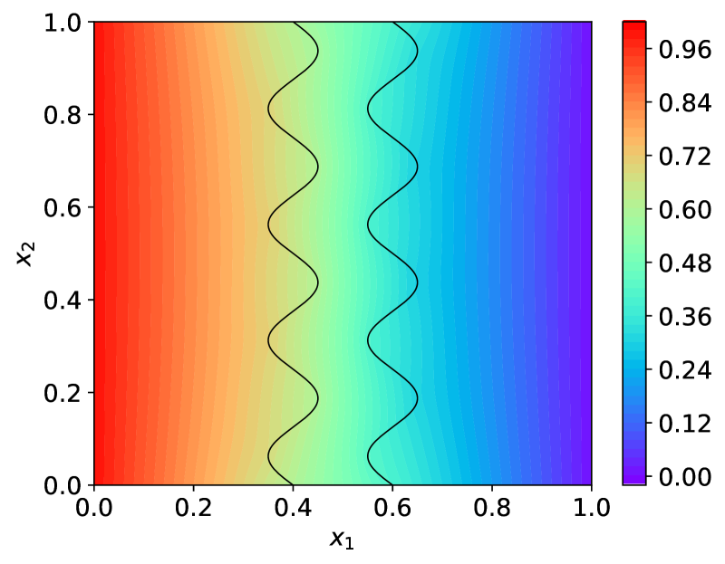
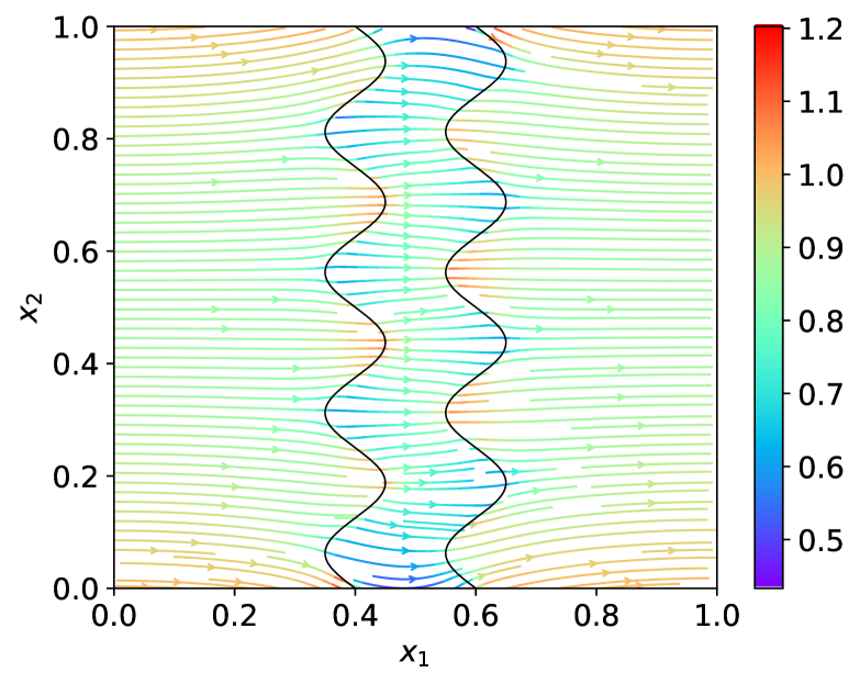
Figure 4: Full-dimensional numerical reference solution (Section 6.1.1) for the pressure $p$ (left) and the velocity $-\mathbf{K}\nabla p$ (right) for the case of $d_{0}=10^{-1}$.

Figure 5 shows the DG solutions for the effective pressure $p_{\Gamma}$ in the reduced models I, I-R, II, and II-R in comparison to the full-dimensional reference solution $p_{\Gamma}^{\mathrm{ref}}$. On the one hand, the effective pressure $p_{\Gamma}=p_{\Gamma}(x_{2})$ is plotted for a fixed valued of $d_{0}=10^{-1}$, where one can see a clear difference between the solutions of the various reduced models. As expected, model I performs best, while model II-R performs worst. On the other hand, Figure 5 also displays the $L^{2}$-error $\smash{{\mathopen{}\mathclose{{}\left\|p_{\Gamma}-p_{\Gamma}^{\mathrm{ref}}}\right\|}_{L^{2}(\Gamma)}}$ as function of the aperture parameter $d_{0}$, where, again, the solution of model I sticks out as the most accurate. In Figure 5, the $L^{2}$-errors of the reduced models I-R and II-R show a similar behavior. In particular, their convergence towards the reference solution $p_{\Gamma}^{\mathrm{ref}}$ for a decreasing aperture is considerably slower than the convergence for the models I and II. Thus, in this test problem, it is primarily the rectification of the bulk domains $\Omega_{1}$ and $\Omega_{2}$ that negatively affects the model error and rate of convergence with respect to a decreasing aperture. However, comparing the solutions of model I and model II, there is also an undeniable effect on the accuracy of the solution in connection with the inclusion of aperture gradients $\nabla d_{1}$, $\nabla d_{2}$ in Eq. 67b. For small apertures, the error of model I seems to stagnate. This is attributed to numerical errors in the computation of the full-dimensional reference solution $p_{\Gamma}^{\mathrm{ref}}$ and discussed in greater detail in Section 6.2.

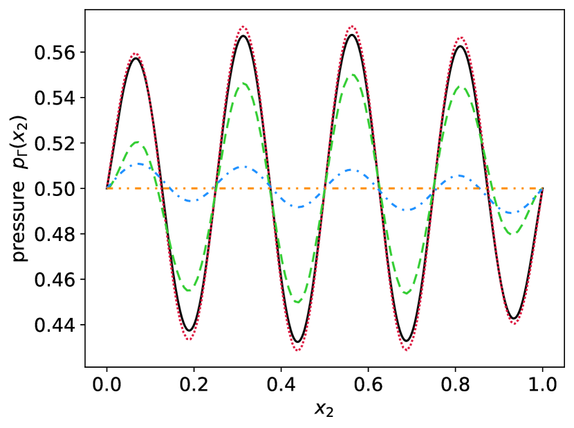
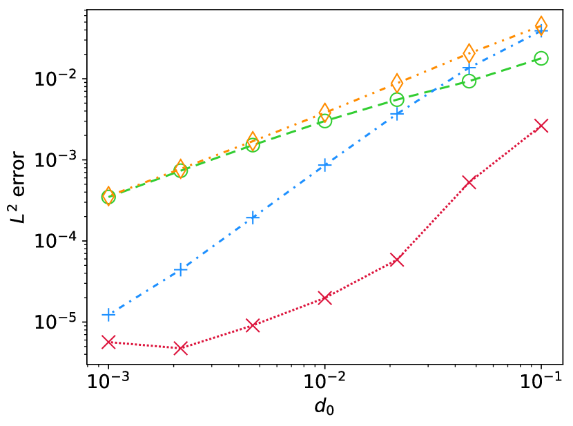
Figure 5: Numerical solutions (Section 6.1.1) for the effective pressure $p_{\Gamma}$ for the reduced model (67) and its variants in comparison to the numerical reference solution $\smash{p_{\Gamma}^{\mathrm{ref}}}$ for $d_{0}=10^{-1}$ (left) and $L^{2}$-error $\|p_{\Gamma}-p_{\Gamma}^{\mathrm{ref}}\|_{L^{2}(\Gamma)}$ as function of $d_{0}$ (right).

6.1.2 Three-Dimensional Test Problem

Next, we extend the test problem from Section 6.1.1 to the three-dimensional case. For this, we define the aperture functions $d_{1}$ and $d_{2}$ by

(84a) $$d_{1}(x_{2},x_{3}) =d_{0}+\tfrac{1}{2}d_{0}\big{(}\sin(8\pi x_{2})+\sin(8\pi x_{3})\big{)},$$

(84b) $$d_{2}(x_{2},x_{3}) =d_{0}-\tfrac{1}{2}d_{0}\big{(}\sin(8\pi x_{2})+\sin(8\pi x_{3})\big{)},$$

with a parameter $d_{0}>0$ so that the total aperture $d(x_{2},x_{3})=2d_{0}$ is constant. The resulting geometry is illustrated in Figure 7. The permeability and boundary conditions are defined as in Section 6.1.1.

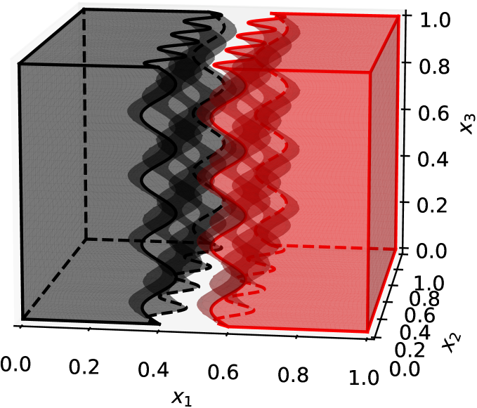
Figure 6: Bulk domains $\Omega_{1}$ (black) and $\Omega_{2}$ (red) (Section 6.1.2) for $d_{0}=10^{-1}$.

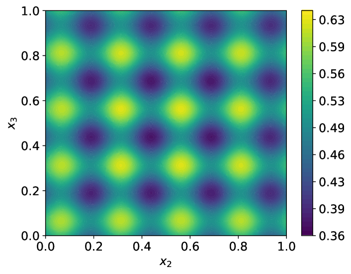
Figure 7: Numerical reference solution $p_{\Gamma}^{\mathrm{ref}}$ (Section 6.1.2) for $d_{0}=10^{-1}$.

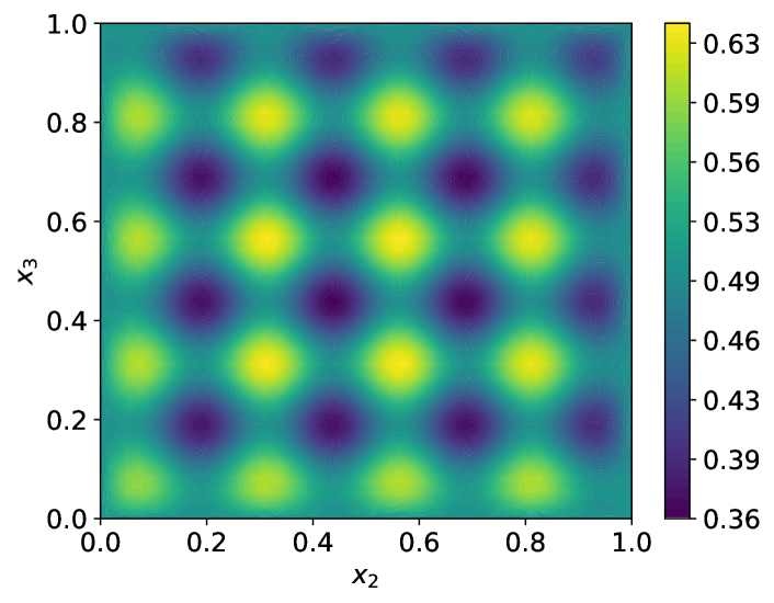
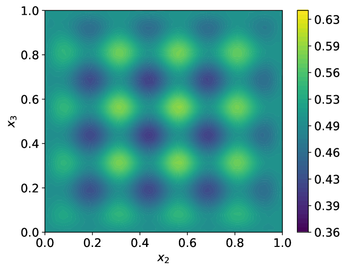
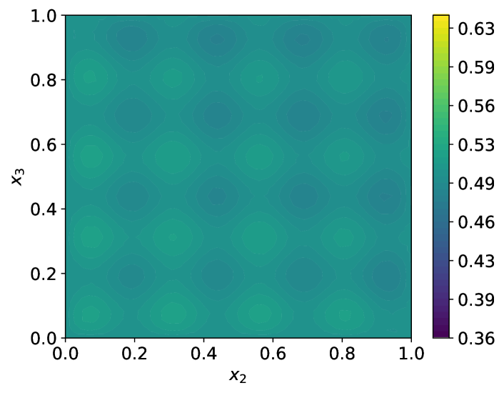
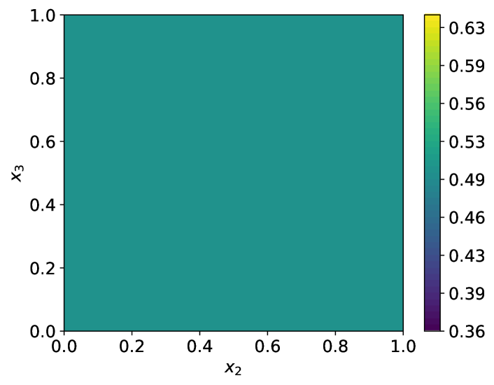
Figure 8: Numerical solutions (Section 6.1.2) for the effective pressure $p_{\Gamma}$ inside the fracture for the reduced model (67) and its variants for $d_{0}=10^{-1}$: model I (top left), model I-R (top right), model II (bottom left), and model II-R (bottom right).

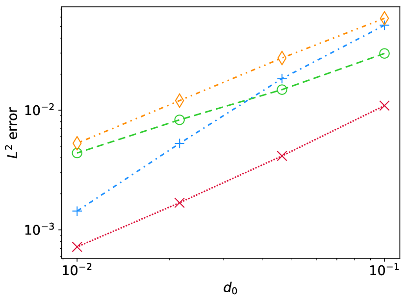
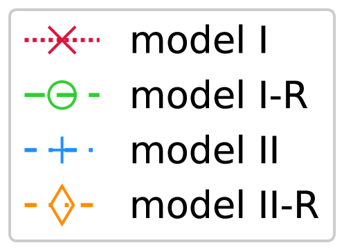
Figure 9: $L^{2}$-error $\smash{\|p_{\Gamma}-p_{\Gamma}^{\mathrm{ref}}\|_{L^{2}(\Gamma)}}$ as function of $d_{0}$ (Section 6.1.2).

Figure 7 displays the numerical reference solution for the averaged pressure $p_{\Gamma}^{\mathrm{ref}}$ for $d_{0}=10^{-1}$. Besides, the DG solutions for the effective pressure $p_{\Gamma}$ in the reduced model (67) and its variants are shown in Figure 8. Here, in comparison with the reference solution in Figure 7, a behavior analogous to the two-dimensional case in Figure 5 becomes apparent. The solution of model I matches well with the reference solution, whereas the solutions of the models I-R and II reproduce the sine-like pattern of the reference solution at a too low amplitude and the solution of model II-R is virtually constant. This is also reflected by the $L^{2}$-error $\smash{{\mathopen{}\mathclose{{}\left\|p_{\Gamma}-p_{\Gamma}^{\mathrm{ref}}}\right\|}_{L^{2}(\Gamma)}}$, which is displayed in Figure 9 as function of the aperture parameter $d_{0}$. The $L^{2}$-error shows the same trends for a declining aperture as observed in the two-dimensional case.

6.2 Flow Perpendicular to an Axisymmetric Fracture

For this next test problem, we again consider a sinusoidal fracture in the two-dimensional domain $\Omega=(0,1)^{2}$, however, this time with a non-constant total aperture $d$. More particularly, the aperture functions $d_{1}$ and $d_{2}$ are defined by

(85) $$d_{1}(x_{2}) =d_{0}+\tfrac{1}{2}d_{0}\sin(8\pi x_{2}),\qquad d_{2}(x_{2})=d_{0}+\tfrac{1}{2}d_{0}\sin(8\pi x_{2})$$

with a free parameter $d_{0}>0$. Thus, the interface $\Gamma$ is the center line of an axisymmetric fracture and the total aperture $d$ ranges between $d_{0}$ and $3d_{0}$. In addition, the permeability $\mathbf{K}_{\mathrm{f}}$ inside the fracture and the given pressure $g$ at the external boundary $\partial\Omega$ are defined as in Section 6.1.1. The fracture geometry and full-dimensional solution from the DG scheme (79) are shown in Figure 10 for the case of $d_{0}=10^{-1}$.

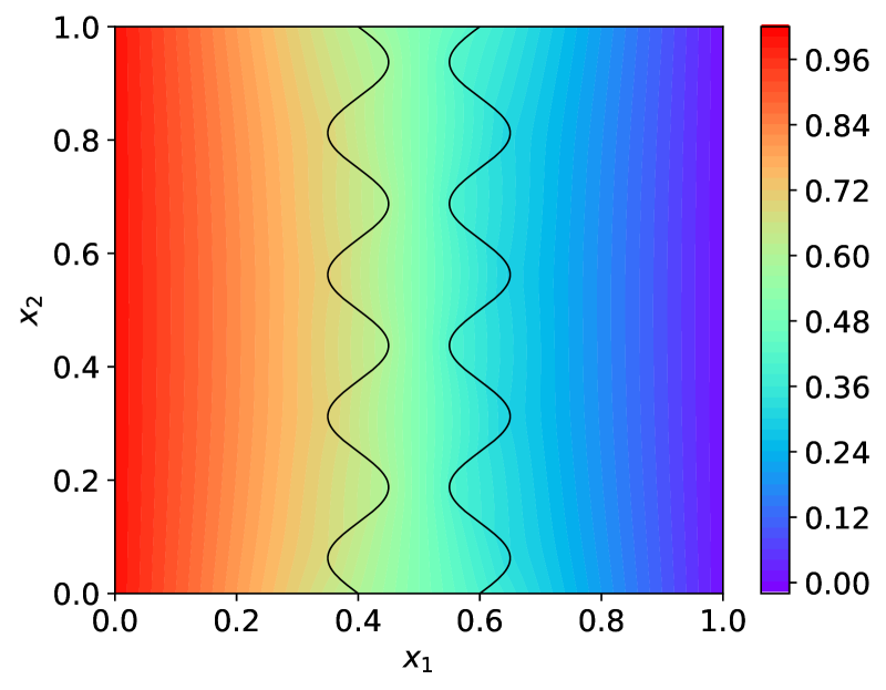
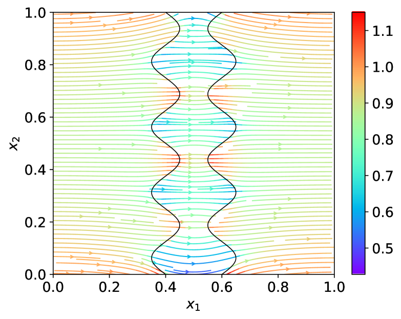
Figure 10: Full-dimensional numerical reference solution (Section 6.2) for the pressure $p$ (left) and the velocity $-\mathbf{K}\nabla p$ (right) for the case of $d_{0}=10^{-1}$.

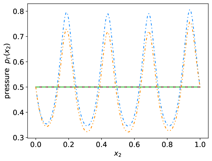
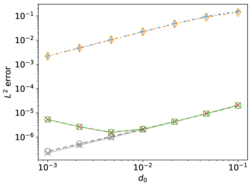
Figure 11: Numerical solutions (Section 6.2) for the effective pressure $p_{\Gamma}$ for the reduced model (67) and its variants in comparison to the numerical reference solution $\smash{p_{\Gamma}^{\mathrm{ref}}}$ for $d_{0}=10^{-1}$ (left) and $L^{2}$-error $\|p_{\Gamma}-p_{\Gamma}^{\mathrm{ref}}\|_{L^{2}(\Gamma)}$ as function of $d_{0}$ (right) with respect to the numerical reference solution $\smash{p_{\Gamma}^{\mathrm{ref}}}$ (in color) and the presumably exact reference solution $p_{\Gamma}^{\mathrm{ref}}\equiv\smash{\frac{1}{2}}$ (gray).

A comparison between the numerical solution $p_{\Gamma}$ of the different reduced models and the averaged full-dimensional reference solution $p_{\Gamma}^{\mathrm{ref}}$ inside the fracture can be found in Figure 11. Here, it occurs that the solutions of the models I and I-R and the solutions of the models II and II-R respectively show a very similar behavior. While the solutions of model II and II-R slowly display convergence towards the reference solution with declining aperture parameter $d_{0}$, there is already a remarkable agreement between the solutions of model I and I-R and the reference solution. As compared to the solutions of model II and II-R, the solutions of model I and I-R are more accurate by several orders of magnitude. Thus, in contrast to the test problem in Section 6.1.1, the artificial rectification of the bulk domains $\Omega_{1}$ and $\Omega_{2}$ is virtually without effect, while the inclusion of aperture gradients $\nabla d_{1}$, $\nabla d_{2}$ in Eq. 67b seems all the more significant in order to obtain accurate solutions. This is probably due to the symmetry of the problem and cannot be expected in general.

Further, it is noticeable in Figure 11 that, for the models I and I-R, the $L^{2}$-error with respect to the numerical reference solution $p_{\Gamma}^{\mathrm{ref}}$ suffers a stop of convergence at small values of the aperture parameter $d_{0}$. Inspecting the numerical reference solution $p_{\Gamma}^{\mathrm{ref}}$ for small apertures, one observes an unphysical oscillatory behavior, which might be associated with the integration of the full-dimensional reference solution according to Eq. 22a. In particular, these spurious oscillations display amplitudes in the range of $10^{-5}$ to $10^{-6}$ and hence can fully explain the total $L^{2}$-error and stop of convergence in Figure 11. Furthermore, the symmetry of the test problem in this section suggests that the effective pressure inside the fracture exactly equals $p_{\Gamma}^{\mathrm{ref}}\equiv\frac{1}{2}$. Thus, we can consider the $L^{2}$-error with respect to this presumably exact solution, which is also shown in Figure 11. Remarkably, in this case, one observes unimpeded convergence with the decline of the aperture parameter $d_{0}$. This confirms that we are dealing with a numerical error in the computation of the reference solution and not with a systematic model error.

6.3 Tangential Flow through an Axisymmetric Fracture

In this test problem, we consider an axisymmetric sinusoidal fracture as in Section 6.2 with the aperture functions $d_{1}$ and $d_{2}$ defined by Eq. 85. Besides, we define the permeability inside the fracture by $\mathbf{K}_{\mathrm{f}}=2\mathbf{I}$ for the full-dimensional model (5), which results in the effective permeabilities $\mathbf{K}_{\Gamma}=2\mathbf{I}$ and $K_{\Gamma}^{\perp}=2$ for the reduced model (67) and its variants. In particular, the fracture permeability is larger than the bulk permeability. The pressure $p$ at the boundary $\partial\Omega$ is given by the function $g({\bm{x}})=4x_{1}(1-x_{1})(1-x_{2})$. This results in an inflow at bottom of the domain with the fracture as the preferential flow path. Figure 12 illustrates the fracture geometry and the resulting solution from the DG scheme (79) for $d_{0}=10^{-1}$.

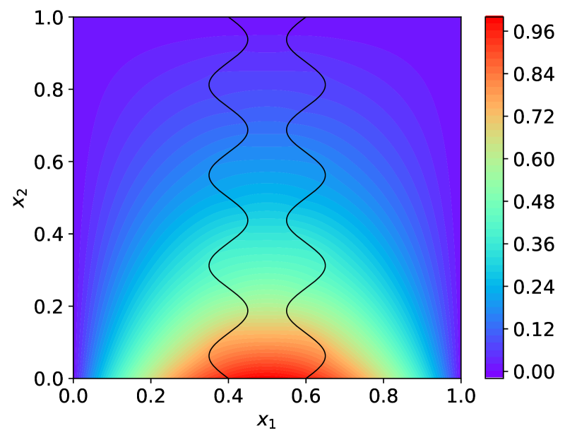
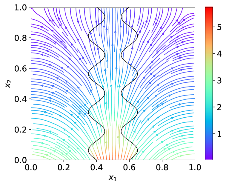
Figure 12: Full-dimensional numerical reference solution (Section 6.3) for the pressure $p$ (left) and the velocity $-\mathbf{K}\nabla p$ (right) for the case of $d_{0}=10^{-1}$.

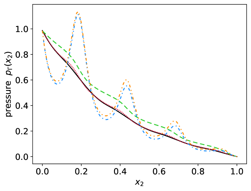
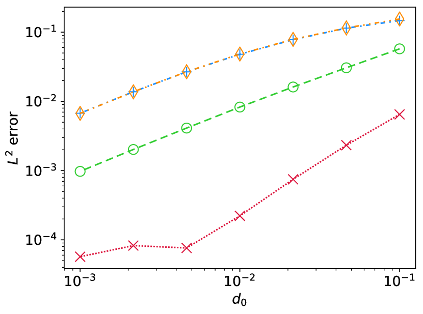
Figure 13: Numerical solutions (Section 6.3) for the effective pressure $p_{\Gamma}$ for the reduced model (67) and its variants in comparison to the numerical reference solution $\smash{p_{\Gamma}^{\mathrm{ref}}}$ for $d_{0}=10^{-1}$ (left) and $L^{2}$-error $\|p_{\Gamma}-p_{\Gamma}^{\mathrm{ref}}\|_{L^{2}(\Gamma)}$ as function of $d_{0}$ (right).

Figure 13 shows the DG solutions $p_{\Gamma}$ of the different reduced models in comparison with the numerical reference solution $p_{\Gamma}^{\mathrm{ref}}$. In particular, it can be seen that the models II and II-R display a similar behavior and are the least accurate, while model I shows the best match with the reference solution. Further, in Figure 13, the $L^{2}$-error $\|p_{\Gamma}-p_{\Gamma}^{\mathrm{ref}}\|_{L^{2}(\Gamma)}$ displays a convergence with the decline of the aperture parameter $d_{0}$ for all variants of the reduced model (67), where the solution of model I converges faster than the solutions of the other models. However, for model I, the convergence stagnates at small apertures, which is associated with numerical errors in the computation of the reference solution $p_{\Gamma}^{\mathrm{ref}}$ as discussed in Section 6.2. Notably, for the test problem in this section, one finds by comparing the solution of model I with the solutions of model I-R and model II in Figure 13 that both the artificial rectification of the bulk domains $\Omega_{1}$ and $\Omega_{2}$ and the negligence of aperture gradients in Eq. 67b significantly impair the accuracy of the solution.

7 Conclusion

In this work, we have derived a new model for single-phase flow in fractured porous media, where fractures are represented as lower-dimensional interfaces. The model accounts for asymmetric fractures with spatially varying aperture and can be viewed as a generalization of a previous model by Martin et al. [22]. The new model allows to study rough-surfaced, possibly curvilinear and winding real-world fracture geometries, while avoiding thin equi-dimensional fracture domains that require highly resolved grids in numerical methods. In various numerical experiments, we have found a remarkable agreement between the solution of the new interface model and the reference profile. Moreover, it has been observed that neglecting any of the terms in the model associated with a varying fracture aperture can substantially impair the accuracy of the solution.

As a future perspective, it is planned to apply the new model to real-world fracture geometries. Future extensions to related interface systems include two-phase flow systems (cf. [10]) and heterogeneous flow systems with different flow models for bulk and fracture domains, e.g., a free-flow regime inside the fracture.

References

- [1] E. Ahmed, J. Jaffré, and J. E. Roberts, A reduced fracture model for two-phase flow with different rock types, Math. Comput. Simul., 137 (2017), pp. 49–70.
- [2] M. S. Alnæs, A. Logg, K. B. Ølgaard, M. E. Rognes, and G. N. Wells, Unified form language: A domain-specific language for weak formulations of partial differential equations, ACM Trans. Math. Softw., 40 (2014), 9, pp. 1–37.
- [3] P. Angot, F. Boyer, and F. Hubert, Asymptotic and numerical modelling of flows in fractured porous media, ESAIM: Math. Model. Numer. Anal., 43 (2009), p. 239–275.
- [4] P. F. Antonietti, C. Facciolà, A. Russo, and M. Verani, Discontinuous Galerkin approximation of flows in fractured porous media on polytopic grids, SIAM J. Sci. Comput., 41 (2019), pp. A109–A138.
- [5] P. Bastian et al., The DUNE framework: Basic concepts and recent developments, Comput. Math. Appl., 81 (2021), pp. 75–112.
- [6] I. Berre, F. Doster, and E. Keilegavlen, Flow in fractured porous media: A review of conceptual models and discretization approaches, Transp. Porous Med., 130 (2019), pp. 215–236.
- [7] I. Berre et al., Verification benchmarks for single-phase flow in three-dimensional fractured porous media, Adv. Water Resour., 147 (2021), 103759.
- [8] W. M. Boon, J. M. Nordbotten, and I. Yotov, Robust discretization of flow in fractured porous media, SIAM J. Numer. Anal., 56 (2018), pp. 2203–2233.
- [9] S. Burbulla, A. Dedner, M. Hörl, and C. Rohde, Dune-MMesh: The Dune grid module for moving interfaces, J. Open Source Softw., 7 (2022), 3959.
- [10] S. Burbulla and C. Rohde, A finite-volume moving-mesh method for two-phase flow in dynamically fracturing porous media, J. Comput. Phys., 458 (2022), 111031.
- [11] A. Dedner, R. Klöfkorn, M. Nolte, and M. Ohlberger, A generic interface for parallel and adaptive discretization schemes: abstraction principles and the DUNE-FEM module, Comput., 90 (2010), pp. 165–196.
- [12] B. Flemisch et al., Benchmarks for single-phase flow in fractured porous media, Adv. Water Resour., 111 (2018), p. 239–258.
- [13] L. Formaggia, A. Fumagalli, A. Scotti, and P. Ruffo, A reduced model for Darcy´s problem in networks of fractures, ESAIM: M2AN, 48 (2014), pp. 1089–1116.
- [14] N. Frih, J. E. Roberts, and A. Saada, Modeling fractures as interfaces: a model for Forchheimer fractures, Comput. Geosci., 12 (2008), pp. 91–104.
- [15] A. Fumagalli, E. Keilegavlen, and S. Scialò, Conforming, non-conforming and non-matching discretization couplings in discrete fracture network simulations, J. Comput. Phys., 376 (2019), pp. 694–712.
- [16] A. Fumagalli and A. Scotti, A mathematical model for thermal single-phase flow and reactive transport in fractured porous media, J. Comput. Phys., 434 (2021), 110205.
- [17] M. Hörl, Flow in porous media with fractures of varying aperture, master’s thesis, University of Stuttgart, 2022.
- [18] M. Hörl, S. Burbulla, and C. Rohde, The mmdgpy Python Package: Source Code and Replication Data for “Flow in Porous Media with Fractures of Varying Aperture”, 2022, https://doi.org/10.18419/darus-3012.
- [19] J. Jaffré, M. Mnejja, and J. Roberts, A discrete fracture model for two-phase flow with matrix-fracture interaction, Procedia Comput. Sci., 4 (2011), pp. 967–973.
- [20] K. Kumar, F. List, I. S. Pop, and F. A. Radu, Formal upscaling and numerical validation of unsaturated flow models in fractured porous media, J. Comput. Phys., 407 (2020), 109138.
- [21] M. Lesinigo, C. D’Angelo, and A. Quarteroni, A multiscale Darcy–Brinkman model for fluid flow in fractured porous media, Numer. Math., 117 (2011), pp. 717–752.
- [22] V. Martin, J. Jaffré, and J. E. Roberts, Modeling fractures and barriers as interfaces for flow in porous media, SIAM J. Sci. Comput., 26 (2005), pp. 1667–1691.
- [23] N. Schwenck, B. Flemisch, R. Helmig, and B. I. Wohlmuth, Dimensionally reduced flow models in fractured porous media: crossings and boundaries, Comput. Geosci., 19 (2015), pp. 1219–1230.