Expert Elicitation and Data Noise Learning for Material Flow Analysis using Bayesian Inference

Abstract

Bayesian inference allows the transparent communication of uncertainty in material flow analyses (MFAs), and a systematic update of uncertainty as new data become available. However, the method is undermined by the difficultly of defining proper priors for the MFA parameters and quantifying the noise in the collected data. We start to address these issues by first deriving and implementing an expert elicitation procedure suitable for generating MFA parameter priors. Second, we propose to learn the data noise concurrent with the parametric uncertainty. These methods are demonstrated using a case study on the 2012 U.S. steel flow. Eight experts are interviewed to elicit distributions on steel flow uncertainty from raw materials to intermediate goods. The experts’ distributions are combined and weighted according to the expertise demonstrated in response to seeding questions. These aggregated distributions form our model parameters’ prior. A sensible, weakly-informative prior is also adopted for learning the data noise. Bayesian inference is then performed to update the parametric and data noise uncertainty given MFA data collected from the United States Geological Survey (USGS) and the World Steel Association (WSA).The results show a reduction in MFA parametric uncertainty when incorporating the collected data. Only a modest reduction in data noise uncertainty was observed; however, greater reductions were achieved when using data from multiple years in the inference. These methods generate transparent MFA and data noise uncertainties learned from data rather than pre-assumed data noise levels, providing a more robust basis for decision-making that affects the system.

Keywords: Prior elicitation and aggregation, Data noise, Bayesian inference, Bayes factor

1 Introduction

Material flow analysis (MFA) is a foundational tool of industrial ecology research [1] and characterizes how a given material is transported and transformed through a supply chain. MFAs are key to identifying potential resource efficiency improvements (e.g., increased recycling), and to evaluating the upstream and downstream system impacts of local interventions; e.g., the potential to reduce greenhouse gas (GHG) emissions released during material production by improving downstream manufacturing process yields [2]. MFAs have been used to help set environmental policies and goals by national governments (e.g., justifying Japan’s reduce, reuse, and recycling laws), local governments (e.g., remedial action taken against toxic releases into New York City harbor), and companies (e.g., Toyota’s corporate MFA was used to set company goals for emissions and recycling) [3]. The proliferation of MFA, however, is hindered by at least two major challenges. First is the long timeline for creating and updating detailed MFAs, currently taking months or even years. Second is the lack of uncertainty quantification (UQ) in most MFA results—a lack of UQ limits insight into the impacts, risks and unintended consequences of system interventions. It is increasingly accepted that UQ must be included in MFA results if they are to meaningful support informed decision- and policy-making [3, 4]. Bayesian methods help address these challenges of UQ and laboriousness in MFA, as explained below.

1.1 Previous work on Bayesian inference in MFA

Bayesian inference is a probabilistic approach to achieve data reconciliation that adjusts MFA variable estimates by combining prior knowledge with collected material flow data [5, 6, 7, 8]. The prior information is typically a combination of fact-based knowledge with subjective impressions based on experience [9]. The prior belief about an MFA variable, such as the mass flow between two processes in a factory, is expressed as a probability density function (PDF); e.g., a Gaussian PDF could be used to represent a prior belief that a mass flow is expected to be 10 $t$ with a variance of 1 $t^{2}$. MFA data are subsequently collected and the “noise” in the collected data—e.g., due to the error in a mass sensor reading—is also expressed as PDFs. In Bayesian inference, the collected MFA data are combined with the priors to generate an updated posterior belief, represented as updated conditional PDFs.

Bayesian inference presents several advantages over other forms of MFA data reconciliation such as least squares optimization [10, 11]. First, it allows a rigorous quantification of uncertainty via the probability and statistics formalism, and allows flexible probability distributions able to capture high-order non-Gaussian and correlation effects. For example, the prior knowledge of an MFA variable might be best represented as a uniform rather than normal distribution if nothing is known other than the upper and lower bounds on the variable. Second, it is particularly suited for handling sparse, noisy, and incomplete data, and can incorporate multiple data streams simultaneously. Third, the Bayesian framework provides a natural entryway to inject domain knowledge, such as by using historical data or opinions from subject matter experts to form the prior distribution of the MFA variables [12]. Bayesian inference can also be “chained” together, to perform sequential learning that iteratively assimilates new data as they become available. Even when little data is available, the Bayesian approach can provide a practitioner with an MFA with associated uncertainties.

Bayesian inference was first used in MFA in 2010 by Gottschalk et al. [13] to study nano-TiO₂ mass flows. They formed uniform and triangular prior distributions centered on values of historical data and performed Bayesian inference using a Metropolis sampling algorithm with simulated instead of measured data. In 2018, Lupton and Allwood [14] introduced additional MFA prior forms (e.g., Dirichlet priors) and conducted a case study on deriving the global steel flow. Their case study highlights some of the challenges of applying Bayesian inference to MFA:

• Assigning proper and rigorously justified prior distributions. Lupton and Allwood’s steel flow analysis [14] used previous results from Cullen et al. [15] as the basis of their priors. However, historical data may not be always available and even when it is (and still deemed relevant) it remains unclear how to form a probability distribution that properly reflects the uncertainty. Assuming a prior variance without justification can introduce bias to the posterior results. Alternatively, non-informative or weakly-informative priors may be used; e.g., assigning a wide uniform PDF for a mass flow between 0 Mt and 200 Mt. However, they will likely require more MFA data to be collected in order to decrease uncertainty to desirable levels.

• Assigning noise to collected MFA data. MFA relevant data are typically published without accompanying uncertainty information; e.g., no error bars are given for the commodity mass flow data reported by the U.N. Comtrade Database [16] or from trade associations such as the World Steel Association [17].

  How then to model the data noise? Assumptions can be made; e.g., Lupton and Allwood [14] assume the data noise in their collected data follows a Gaussian distribution with a standard deviation equal to 10% of the observed value. Such assumptions can introduce bias into the final posterior MFA results and provide a false sense of confidence if the assumed noise over-estimates the data quality. Elsewhere, there are qualitative methods to categorize data into uncertainty levels based on features such as the perceived data source quality and specificity [18], and semi-quantitative approaches such as using a pedigree matrix or confidence score [19, 11] which translates an uncertainty level into a probability distribution or numerical value. The strict quantitative identification of MFA data uncertainty has been lacking so far [20]; however, the Bayesian framework can also facilitate the learning of data noise.

1.2 Scope and structure of this article

This paper explores how to: (a) Form informative prior distributions for MFA variables by eliciting information from industrial experts, and (b) Learn the data noise from collected data by incorporating data noise as random variables for inference. In Sec. 2, we first introduce the MFA problem mathematically using the conservation of mass principle (Sec. 2.1) and then formulate Bayesian inference for learning MFA model parameters and the collected data noise (Sec. 2.2). The two crucial components needed for solving a Bayesian inference problem—the likelihood and prior—are then presented in Sec. 2.3 and 2.4 respectively. In particular, Sec. 2.4 reviews existing methods for expert elicitation and discusses their use for the MFA framework. In Sec. 3, we apply these methods to derive the U.S. steel flow for 2012. Finally, in Sec. 4 we discuss the lessons learned from the case study.

2 Formulation

2.1 A Mathematical Representation of MFA

An MFA can be represented via a directed graph as shown in Fig. 1. The nodes of the graph (indexed by $1,2,\ldots,n_{p}$) represent different processes, products or locations. Each directed edge connecting two nodes represents the mass flow of material from one process to another.

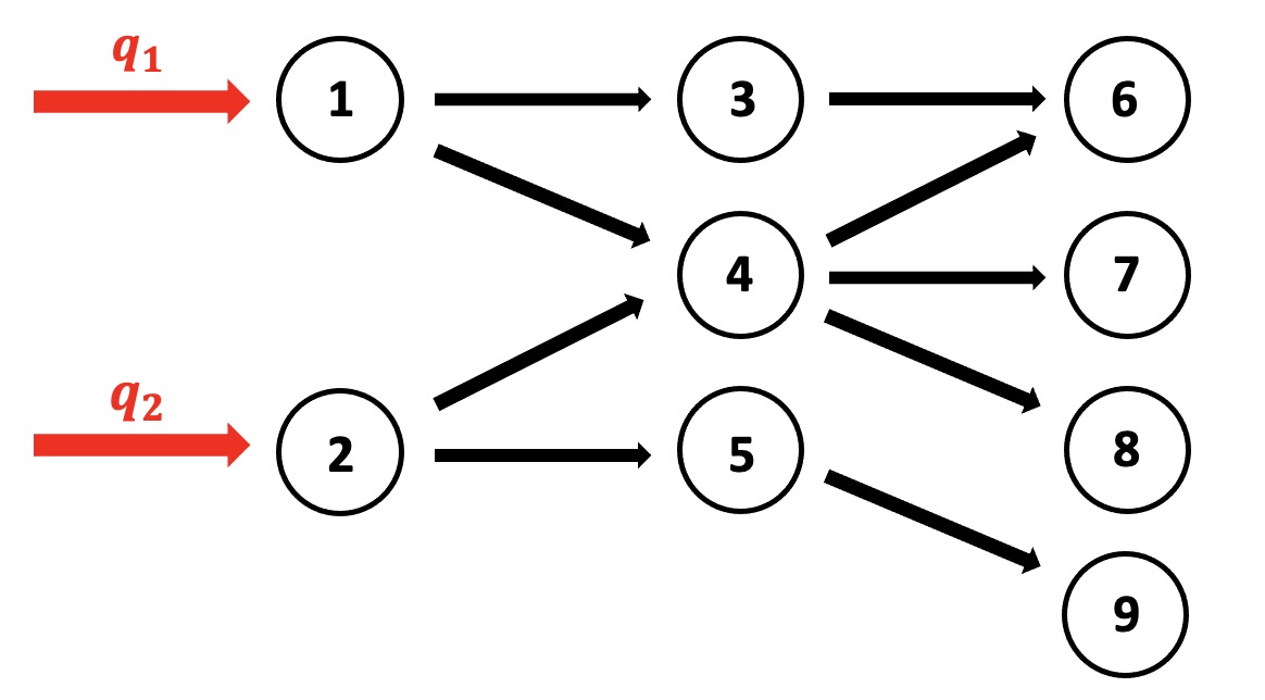
Figure 1: A graphical representation of an MFA network structure

At the core of MFA is the conservation of mass, which requires the total input flow of material mass for each node to equal its total output flow. We denote the total input (equivalently, total output) flow for node $i$ by $z_{i}$. The flow along an edge out of node $i$ (e.g., to node $j$) is then equal to $\phi_{ij}z_{i}$, where $\phi_{ij}\in[0,1]$ is the allocation fraction of node $i$’s total outflow going into node $j$ ($\phi_{ij}=0$ if there is no flow from node $i$ to node $j$). Hence,

$$\sum_{i=1}^{n_{p}}\phi_{ij}z_{i}=z_{j}.$$ (1)

Furthermore, for each node, its output allocation fractions need to sum to unity:

$$\sum_{j=1}^{n_{p}}\phi_{ij}=1.$$ (2)

We recommend working with the allocation fractions ($\phi_{ij}$) as model parameters instead of working directly with the mass flow values for each edge. The allocation fractions offer a convenient method of expressing and allowing the mass balance relationships for the entire MFA to be assembled into a linear system as proposed by Gottschalk et al. [21]. For instance, the mass balance equations for the simple MFA shown in Fig. 1 can be expressed as:

$$\underbrace{\begin{bmatrix}1&0&0&0&0&0&0&0&0\\ 0&1&0&0&0&0&0&0&0\\ -\phi_{13}&0&1&0&0&0&0&0&0\\ -\phi_{14}&-\phi_{24}&0&1&0&0&0&0&0\\ 0&-\phi_{25}&0&0&1&0&0&0&0\\ 0&0&-\phi_{36}&-\phi_{46}&0&1&0&0&0\\ 0&0&0&-\phi_{47}&0&0&1&0&0\\ 0&0&0&-\phi_{48}&0&0&0&1&0\\ 0&0&0&0&-\phi_{59}&0&0&0&1\\ \end{bmatrix}}_{\mathbb{I}-\Phi^{T}}\underbrace{\begin{bmatrix}z_{1}\\ z_{2}\\ z_{3}\\ z_{4}\\ z_{5}\\ z_{6}\\ z_{7}\\ z_{8}\\ z_{9}\\ \end{bmatrix}}_{z}=\underbrace{\begin{bmatrix}q_{1}\\ q_{2}\\ 0\\ 0\\ 0\\ 0\\ 0\\ 0\\ 0\\ \end{bmatrix}}_{q}$$ (3)

where $\mathbb{I}$ is the $n_{p}\times n_{p}$ identity matrix, $\Phi\in\mathbb{R}^{n_{p}\times n_{p}}$ is the adjacency matrix where entries are the allocation fractions $\phi_{ij}$, $z\in\mathbb{R}^{n_{p}}$ depicts all the nodal mass flows, and $q\in\mathbb{R}^{n_{p}}$ represents the external inflows to the network. The material inflows ($q_{i}$) originate from outside the network. For example, a material inflow to the U.S. aluminum material flow network could be imports of aluminum billet.

For a scenario with given $\Phi$ and $q$, we can compute the model prediction for all nodal mass flows via:

$$z=(\mathbb{I}-\Phi^{T})^{-1}q.$$ (4)

Subsequently, from the values of $\{z,\Phi,q\}$, other common MFA quantities of interest (QoIs) can be predicted, such as mass flows for each edge ($\phi_{ij}z_{i}$), and sums, products and ratios of mass flows. We express these QoIs as a function, $G(\phi,q)$, where $\phi$ denotes a flattened vector containing all $\phi_{ij}$’s.

2.2 Bayesian Parameter Inference

Given an MFA model, the set of all unknown MFA parameters $\theta\in\mathbb{R}^{n_{\theta}}$ and the collected MFA data $y\in\mathbb{R}^{n_{y}}$ are treated as random variables and associated with a joint PDF $p(\theta,y)$. Here, we use $\theta$ to denote all MFA model parameters we are interested to learn, which may encompass $\phi$ and $q$ as well as other parameters; $y$ is the flattened set of collected and noisy MFA data records that correspond to the model prediction QoIs $G(\phi,q)$. Bayes’ rule then directly follows from the axioms of probability, stating:

$$p(\theta|y)=\frac{p(\theta,y)}{p(y)}=\frac{p(y|\theta)p(\theta)}{p(y)},$$ (5)

where $p(\theta)$ is the prior PDF representing the initial belief in the MFA parameters $\theta$ before having collected any MFA data; $p(y|\theta)$ is the likelihood PDF (see Sec. 2.3); $p(\theta|y)$ is the posterior PDF representing the updated belief in the MFA parameters $\theta$ after having collected the MFA data $y$; and $p(y)$ is the model evidence (marginal likelihood) and acts as a normalizing constant for the posterior PDF. Performing Bayesian parameter inference entails computing or characterizing the posterior $p(\theta|y)$ while accessing the likelihood and prior.

2.3 Modeling the Likelihood $p(y|\theta)$

The likelihood computes the probability of having collected MFA data $y$ if the model parameters had the value equal to $\theta$; that is, it provides a probabilistic measure on the mismatch between observation $y$ and model prediction $G(\phi,q)$. There are many ways in which the collected data $y$ may relate to $G(\phi,q)$. For example, the discrepancy may be viewed as an additive noise:

$$y_{k}=G_{k}(\phi,q)+\epsilon_{k},$$ (6)

where $k$ indicates the $k$th data component. Equation 6 is appropriate for MFA data where the error is insensitive to the scale of the measurement; e.g., in the case of a mass sensor which has a sensitivity of $\pm$ 10 grams across its measurement range. However, oftentimes the data error increases with the scale of the measurement and can be modeled as a relative noise in the form:

$$y_{k}=G_{k}(\phi,q)(1+\epsilon_{k}).$$ (7)

In either case, modeling the noise $\epsilon_{k}$ as a Gaussian centered around zero is a sensible assumption. For its standard deviation $\sigma_{k}$, we do not presume its magnitude and will instead learn these values from the data. In the absence of information to the contrary, the noise associated with different pieces of data can be modeled as independent. Therefore, if adopting the relative error form in Eqn. 7 and with the unknown model parameters $\theta=\{q,\phi,\sigma\}$, the likelihood PDF is:

$$p(y|\theta)=p_{\epsilon}\left(\frac{y}{G(\phi,q)}-1\right)=\prod_{k=1}^{n_{y}}\frac{1}{\sqrt{2\pi}\sigma_{k}}\exp\left\{-\frac{\left(\frac{y_{k}}{G_{k}(\phi,q)}-1\right)^{2}}{2\sigma_{k}^{2}}\right\}.$$ (8)

2.4 Expert Prior Elicitation for MFA

The goal of expert prior elicitation is to extract pertinent knowledge for $\theta$ from subject matter experts in a form that can used as a proper Bayesian prior PDF. There are two main challenges in expert prior elicitation. An expert does not typically have a preexisting quantification of her belief in the form of a PDF [22]. Therefore, the first challenge is how to elicit and synthesize a single expert’s knowledge into a “quantified belief prior” [22]. Next, when there are multiple experts available, it is desirable to utilize all their opinions to have the prior capture the full diversity of background knowledge. However, Bayesian inference requires a single PDF for a parameter as the prior rather than multiple distributions from several experts. The second challenge is, therefore, how to combine and weight the beliefs of multiple experts into a single prior for each MFA variable of interest.

Expert prior elicitation has been widely applied in medicine to design clinical trials [23], assess the effect of specific treatments for rare disorders [24], and inform health-care decision-making [25]. Prior elicitation has also been used in environmental assessments to forecast future wind energy costs [26] and regional climate change [27]. There has been some preliminary work on expert elicitation in MFA: Montangero and Belevi [28] use expert elicitation to describe the uncertainty regarding the flow of nitrogen and phosphorus in a septic tank. In their work, multiple experts provide uncertainty information as quantiles and their opinions are combined using equal weights. Elsewhere, Mathieux and Brissaud [29] conduct expert elicitation to understand where aluminum is being used in commercial vehicles. In their work, experts are brought together to determine collectively a single distribution for each estimate. In this work, we examine methods for eliciting, weighting, and aggregating multiple experts’ beliefs under the Bayesian framework.

2.4.1 Eliciting a Prior from an Expert

Prior elicitation is typically performed using surveys conducted either remotely (e.g., by mail or online), in-person, or via a hybrid format where the expert is assisted by telephone or video conference [30]. While the variable of interest $\theta$ can be multivariate (e.g., a joint distribution on all the allocation fractions leaving a node), eliciting multi-dimensional PDFs directly is very challenging; therefore, multivariate elicitation typically involves eliciting and then combining univariate marginal distributions [31, 32]. The common methods to elicit univariate PDFs are either a Variable Interval Method or a Fixed Interval Method [32, 33]. In a Variable Interval Method, the expert provides estimates of the quantiles; e.g., estimate $a$ and $b$ such that $\mathbb{P}(\theta\leq a)=0.25$, $\mathbb{P}(a<\theta\leq b)=0.5$ and $\mathbb{P}(b>\theta)=0.25$ [34, 35]. In Fixed Interval Methods, the expert estimates the probability of $\theta$ within given fixed intervals (e.g., estimate $\mathbb{P}(a<\theta\leq b)$ for some given ${a}$ and $b$) [36]. While it is unclear which set of methods yield more accurate representations of the expert’s true belief (Abbas’ findings contradicting those of Murphy and Winkler [37, 34]) it does appear that participants find the Fixed Interval Method easier to complete [37]. Given that many MFA industry experts might be unfamiliar with statistical concepts such as quantiles, we recommend using the Fixed Interval Method for MFA prior elicitation where possible; e.g., for eliciting allocation fractions ($\phi$) which are bounded within $[0,1]$. Elsewhere, when eliciting external inflows ($q$) or data noise parameters ($\sigma_{k}$), there is no upper bound a priori so that it is appropriate to either ask the expert to specify an upper bound before defining the intervals used in the Fixed Interval Method or else use a Variable Interval Method (see SI Section 1).

2.4.2 Prior Aggregation from Multiple Experts

The typical methods for combining multiple experts’ knowledge into a single proper prior PDF are behavioral aggregation and mathematical aggregation [32].

Behavioral Aggregation:

Experts collaborate to define agreed upon priors [32]. Thus, very ‘informed’ experts have the chance to share their knowledge. However, it can be difficult to find a common time when all the experts are available and there are potential issues with strong personalities dominating the decision-making [32], the risk of overconfidence in the group [38], some experts concealing their true views [39, 40], group polarisation [39, 40], and individuals with unique information being ineffective at sharing [41]. Therefore, methods such as the Delphi method [42, 43] and its variants [44, 45] have been proposed where direct interaction between the experts is restricted to prompt the experts to explain their views rather than relying on reputation or personality [32]; e.g., experts may share their views anonymously, adjust their views based on the received information, and iterate until convergence on a distribution.

Mathematical Aggregation:

A distribution is elicited from each of the $n_{e}$ experts independently, yielding $n_{e}$ PDFs $\{p_{1}(\theta),\ldots,p_{n_{e}}(\theta)\}$. An aggregated PDF $p(\theta)$ is then calculated using either linear or logarithmic pooling [32, 46, 47]:

$$\mathrm{(linear)\hskip 20.00003pt}p(\theta)=\sum_{\ell=1}^{n_{e}}w_{\ell}p_{\ell}(\theta),\hskip 60.00009pt\mathrm{(logarithmic)\hskip 20.00003pt}p(\theta)=\frac{1}{Z}\prod_{\ell=1}^{n_{e}}p_{\ell}(\theta)^{w_{\ell}},$$ (9)

where $w_{\ell}$ is the weight associated with expert ${\ell}$, and $Z$ is a normalization constant. In logarithmic pooling, the resulting prior $p(\theta)=0$ whenever any of the experts believe $p_{{\ell}}(\theta)=0$. In contrast, the prior generated by linear pooling includes any value considered plausible by any of the experts and is therefore more conservative in terms of not ruling out experts’ beliefs (see Fig. 2). While equal weights could be assigned to all experts such that $w_{\ell}=1/n_{e}$, it is often desirable to allocate greater weighting to more informed experts, typically using either Social Network Weighting or methods requiring questions on seeding variables, also referred to as seeding questions from hereon. Social Network Weighting assigns weights based on each expert’s number of citations [48] or a consensus among the experts on whose opinion should receive the most weight [49]. Such methods have been criticized for often excluding experts with predominately industry rather than academic experience and for resulting in prior PDFs with low accuracy [48, 49, 50]. Seeding questions assess each expert’s expertise by comparing the experts’ responses to collected seeding variable observations. One seeding variable example for a steel MFA study might be on the fraction of U.S. pig iron consumed in Indiana within a certain time period. The experts’ responses are compared to the observations from a credible source (e.g., USGS). Typically, Cooke’s method [51] is used to convert expert seeding question responses to expert weights where, for expert ${\ell}$, the weight $w_{\ell}\propto C_{\ell}K_{\ell}$ with $C_{\ell}$ being the calibration score and $K_{\ell}$ the information score. The calibration score measures the accuracy of the expert’s responses, and the information score penalizes experts weakly informative responses that approach the uniform distribution. The Kullback-Leibler (KL) divergence is used in calculating both scores. The KL divergence is a measure of how two PDFs differ. It is non-symmetric and non-negative with a KL divergence being zero between two identical distributions, and a larger KL divergence implying a greater difference between two distributions [52]. For discrete variable $X$ taking values in $\{1,2,...,m\}$, and two probability mass functions $P(x)=p_{x}$ and $Q(x)=q_{x}$, the KL divergence from $Q$ to $P$ is given as:

$$\centering D_{\mathrm{KL}}(P||Q)=\sum_{i=1}^{m}p_{i}\ln\left(\frac{p_{i}}{q_{i}}\right).\@add@centering$$ (10)

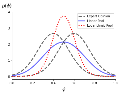
Figure 2: Linear versus logarithmic pooling of two equal weight elicited priors for an allocation fraction ($\phi$). In general, the logrithmic pool result is more “concentrated” than the linear pool result [32].

Each expert’s information score $K_{\ell}$ is calculated as the KL divergence from the expert’s elicited distribution to the uniform distribution, averaged across all the seeding questions (see Fig. 3a). In order to calculate an expert’s calibration score $C_{\ell}$, each response to the seeding questions from expert ${\ell}$ is split into inter-quantile intervals. Typically, four inter-quantile intervals (3 degrees of freedom) are adopted with a corresponding probability vector $Q=\{0.05,0.45,0.45,0.05\}$. Each seeding variable observation is then compared to the inter-quantile intervals derived from the expert’s response; e.g., the USGS records that 34.9% of U.S. pig iron was consumed in Indiana from 2002–2016, falling into the 50–95% interval of the response from expert $\ell$ shown in Fig. 3b. Then, let $P_{\ell}=\{p_{1},p_{2},p_{3},p_{4}\}$ denote the fraction of all $n$ seeding variable observations that fall into each of the four intervals elicited from expert ${\ell}$. Cooke [51] states that for a well-informed “ideal” expert (i.e. where seeding variable observations appear as independently drawn from a distribution consistent with the expert’s quantiles) then $P_{\ell}$ tends to $Q$, and $D_{\mathrm{KL}}(P||Q)$ tends to zero. Cooke defines the calibration score $C_{\ell}$ as the probability that a random variable following a Chi-square distribution (with 3 degrees of freedom if using four inter-quantile intervals) is greater than the likelihood ratio statistic ($2\times n\times D_{\mathrm{KL}}(P||Q)$), see Fig. 3b; therefore, if expert ${\ell}$’s knowledge differs from the seeding variable observations to a large extent, the associated KL divergence would be high and $C_{\ell}$ becomes small. While not discussed previously, we believe that Cooke’s method of calculating $C_{\ell}$ is only appropriate when there is uncertainty in the seeding variable observation (see SI Section 2.4 for a detailed discussion). Eggstaff et al. state that there is no definitive minimum number of seeding questions; however, regardless of the number of questions, Cooke’s method significantly outperforms equally weighting the experts’ judgments [53].

Once the expert weights are computed, they can then be used to carry out the mathematical aggregation in Eqn. 9 to complete the prior construction.

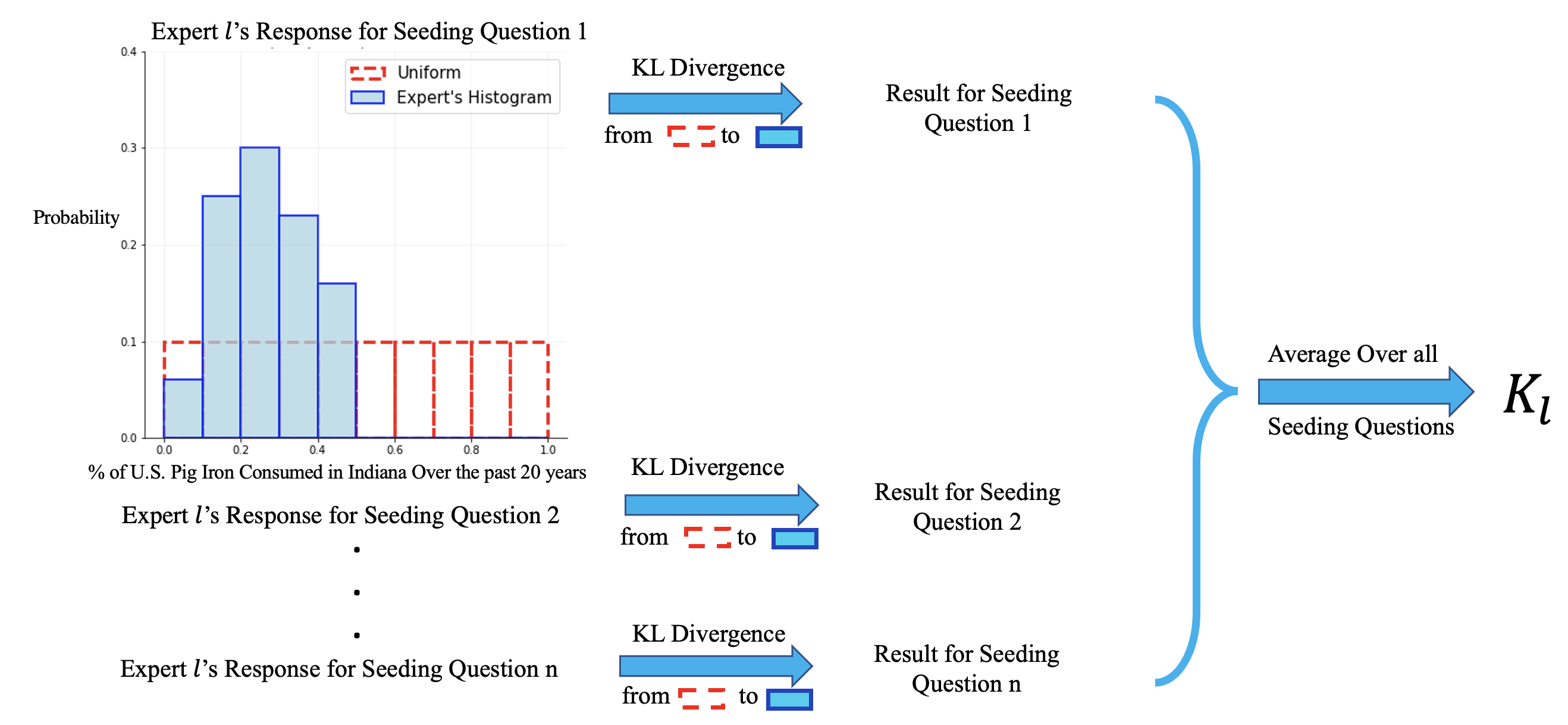
(a) Calculating the information score for an expert.

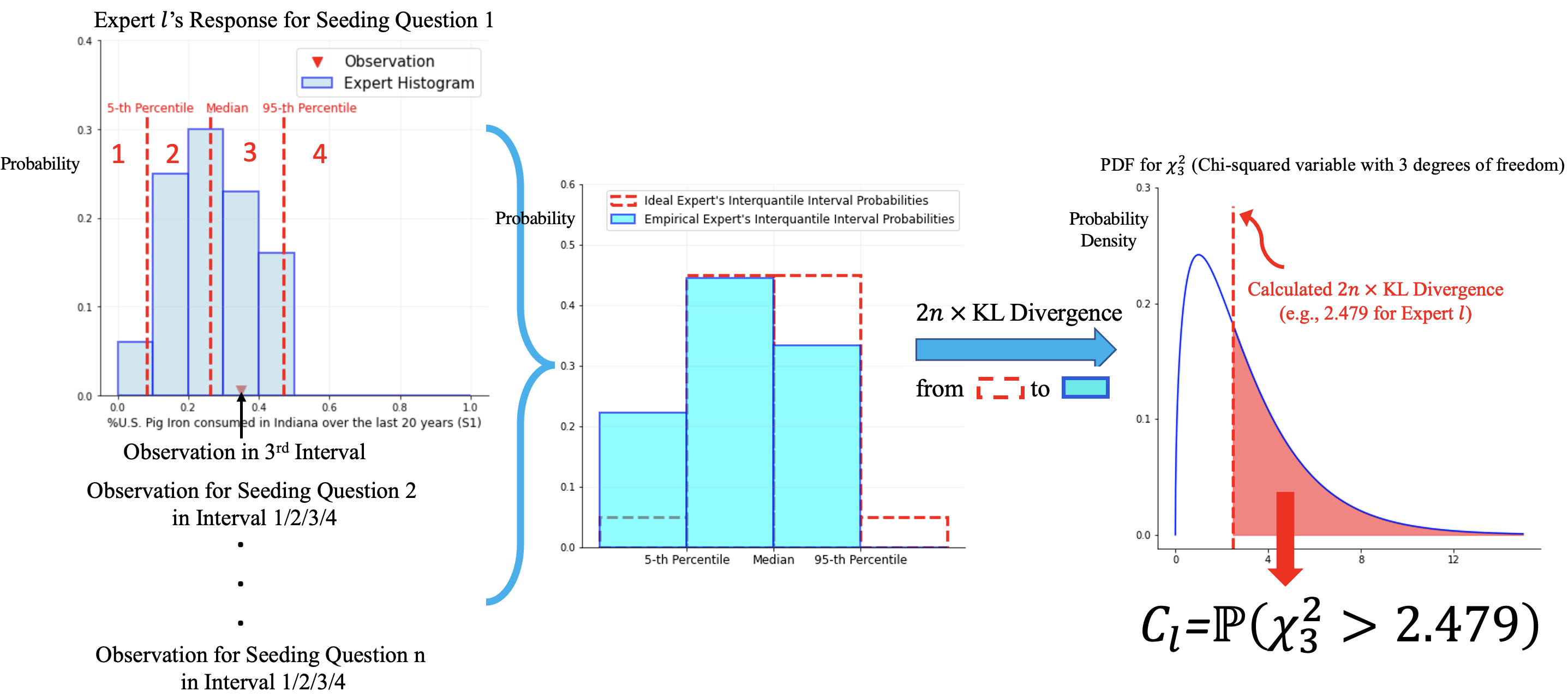
(b) Calculating the calibration score for an expert.

Figure 3: (a) Each expert’s information score $K_{\ell}$ is calculated as the KL divergence from the expert’s elicited histogram to the uniform distribution averaged across all seeding question responses. (b) Each expert’s calibration score $C_{\ell}$ is calculated by first counting the number (fraction) of actual observations of the seeding questions in each inter-quantile interval across all seeding question responses from an expert, then computing the KL divergence from the ideal expert’s inter-quantile interval probabilities to the empirical expert’s inter-quantile interval probabilities, and lastly obtaining the likelihood ratio statistic with the corresponding $p$-value (i.e. $\mathbb{P}(\chi_{3}^{2}>2.479)$ in the above example) being the calibration score.

2.5 Distributions for Modeling the MFA Priors

The next step is fitting the histograms elicited from the MFA experts to a family of parameterized PDFs. The distribution and corresponding hyper-parameters are typically fitted and selected via a least squares procedure [54, 55].

2.5.1 Distributions for Allocation Fraction Priors

Lupton and Allwood [14] proposed using a Dirichlet distribution as the prior for the allocation fractions $\{\phi_{S,d_{1}},...,\phi_{S,d_{S}}\}$ from source node $S$, ensuring that all the allocation fractions remain in $[0,1]$ and sum to unity. The Dirichlet PDF for $\phi_{S,d_{1}},...,\phi_{S,d_{S}}$ given hyper-parameters $\alpha_{D}=\{\alpha_{d_{1}},...,\alpha_{d_{S}}\}$ is

$$p(\phi_{S,d_{1}},...,\phi_{S,d_{S}}|\alpha_{D})=\frac{\Gamma\left(\sum_{i=d_{1}}^{d_{S}}\alpha_{i}\right)}{\prod_{j=d_{1}}^{d_{S}}\Gamma(\alpha_{j})}\prod_{k=d_{1}}^{d_{S}}\phi_{S,k}^{\alpha_{k}-1}$$ (11)

and for each $\phi_{S,i}$, its marginal PDF follows a Beta distribution characterized by

$$p(\phi_{S,i}|\alpha_{D})=\frac{\Gamma\left(\sum_{j=d_{1}}^{d_{S}}\alpha_{j}\right)}{\Gamma(\alpha_{i})\Gamma\left(\sum_{k\neq i}\alpha_{k}\right)}\phi_{S,i}^{\alpha_{i}-1}(1-\phi_{S,i})^{(\sum_{l\neq i}\alpha_{l})-1}.$$ (12)

Another benefit of using a Dirichlet distribution is that eliciting each marginal distribution on $\phi_{S,i}$ (Eqn. 12) from an expert is sufficient to fully construct the Dirichlet joint distribution (Eqn. 11) [32]. After eliciting each marginal histogram of $\phi_{S,i}$ from the experts, we fit for the optimal Dirichlet hyper-parameters $\alpha_{D}^{\ast}$ by minimizing the squared differences between the probability of each Beta marginal that corresponds to the Dirichlet joint distribution and the marginal weighted histograms with $n_{b}$ intervals from the experts, summed across all $d_{S}$ allocation fractions emanating from a source node $S$ [56]:

$$\alpha_{\mathcal{D}}^{\ast}=\operatornamewithlimits{argmin}_{\alpha_{\mathcal{D}}}\sum_{d_{s}=d_{1}}^{d_{S}}\sum_{i=1}^{n_{b}}\left[F(\theta_{d_{s},i+1}|\alpha_{\mathcal{D}})-F(\theta_{d_{s},i}|\alpha_{\mathcal{D}})-\mathbb{P}(\theta_{d_{s},i})\right]^{2},$$ (13)

where $F$ is the Beta CDF.

Other methods exist that may also be used to model the allocation fraction priors [14, 57]. For example, softmax transformations offer extra flexibility compared to using Dirichlet priors; e.g., they can incorporate a strong belief that $\phi_{S,d_{1}}=\phi_{S,d_{2}}$ while the relationship between other allocation fractions is unknown. However, the increased complexity of the procedure complicates the elicitation process because, for example, the CDF in Eqn. 13 cannot be evaluated in a closed-form.

2.5.2 Distributions for Data Noise Parameter Priors $\sigma_{k}$

Since $\sigma_{k}$ is the standard deviation of Gaussian distributed $\epsilon_{k}$, the prior must take positive support; i.e., $p(\sigma_{k}<0)=0$. A common choice of prior for the standard deviation of a Gaussian distribution is the Inverse-Gamma distribution, which enables an analytical evaluation of the posterior when the measured data is linear in the parameters of interest [58]. However, the Inverse-Gamma and other commonly used positive support distributions such as the Log-Normal distribution place negligible probability of $\sigma$ at regions close to zero, greatly reducing the possibility that the MFA data is of high quality. We believe that generally in MFA there should be a moderate probability that the collected data is clean and high quality. Consequently, other prior distributions that place non-negligible probability at regions close to zero should be considered. Such distributions include the half-Cauchy distribution, uniform distribution, and truncated normal distribution.

2.5.3 Distributions for Mass Inflow Priors $q$

The mass inflows $q$ to the network must be positive. Therefore, uniform and truncated normal distributions can be used. When there is little information about $q$, the upper bound can be set to a large value for both distributions. Alternatively, both the half-Cauchy and truncated normal distribution can be used without an upper bound, and set such that the shape of $p(q)$ is close to being flat.

2.6 Posterior Sampling

Once the prior and likelihood are established, the Bayesian inference problem can be solved as stated in Eqn. 5, updating our knowledge about our model parameters through the posterior distribution. Attempting to compute the posterior PDF would entail evaluating the denominator (model evidence) in Bayes’ rule: $p(y)=\int p(y|\theta)p(\theta)\,d\theta$, a task that is generally intractable to perform even numerically except for very low (e.g., $<3$) dimensions of $\theta$. Instead of computing the PDF, a major alternative strategy is to generate samples of $\theta$ from the posterior distribution. To that end, Markov Chain Monte Carlo (MCMC) algorithms [59, 60, 61, 62] have become the predominant methods for computational Bayes in moderate $\theta$ dimensions (e.g., up to $\sim 100$), which iterates a Markov chain to generate samples that are consistent with the targeted posterior distribution. The more scalable MCMC methods include Hamiltonian Monte Carlo (HMC) based samplers such as the No-U-Turn (NUTs) algorithm, which explore the parameter space efficiently leveraging the posterior gradient and Hamiltonian energy principles [63]. However, HMC suffers from divergence in its time integration step when encountering neighborhoods of high posterior curvature [63, 64]; this difficulty was indeed observed in our study when incorporating the data noise parameters $\sigma$ into the Bayesian inference. Therefore, we opt to use sequential Monte Carlo (SMC) [65] to sample the posterior, which is based on the idea of iteratively re-weighing the samples using on a tempered likelihood $[p(y|\theta)]^{\beta}$ at each stage where $\beta$ is a tempering parameter that gradually increases from 0 to 1. We describe the SMC algorithm in SI Section 4.

3 Case Study on the U.S. Steel Flow

The advances in the Bayesian inference approach to MFA discussed above are tested by mapping the U.S. annual flow of steel, where we take the MFA network structure from Zhu et al.’s [11] analysis of U.S. steel flows in 2014. The case study demonstrates rigorous prior development based on expert elicitation and inference of the MFA collected data noise as well as the MFA flow parameters. All the data and code used in this case study are available online (see the SI).

In this case study, the parameters requiring prior formulation are the allocation fractions ($\phi$), the external inputs ($q$), and the data noise standard deviation ($\sigma$) associated with data noise ($\epsilon$).

3.1 Constructing Priors for Allocation Fractions ($\phi$) and Input Flows ($q$)

Since the elicitation of informative priors for all MFA variables of interest can be time prohibitive, we only elicit expert priors for the upstream allocation fractions ($\phi$) and external inputs ($q$), while using weakly informative priors elsewhere. Experts on U.S. steel flows were identified by conducting a literature search on steel flows and recycling and by contacting U.S. steel companies (e.g., U.S. Steel and Nucor). All the experts had more than 5 years of working or research experience in the steel industry. Eight experts agreed to an emailed request to take part in the study (see Table 2 in the SI).

For prior construction, the experts independently completed surveys online that contained a total of 32 questions: 23 elicitation questions for allocation fractions associated with import, export, production and consumption of ferrous raw materials, and an extra 9 seeding questions whose actual observations are taken from USGS.

At least one author was present online to answer any questions during survey completion. It took the experts between 25 and 80 minutes each to complete the survey. The Fixed Interval Method was used to elicit the parameters. For allocation fractions $\phi$, the support $[0,1]$ for $\phi$ was divided into 10 equal-width intervals and Dirichlet hyperparameters were fit to the elicited experts’ histograms as described in Sec. 2.4. For the external inputs, the expert first specifies the lower and upper bound, with the interval then divided into 10 equal-width intervals. Figure 4 shows an illustrative example of a survey question for eliciting an allocation fraction. An expert could enter the probability value for each interval in the box or else drag the bar across for the given interval until the summation of the bars is 1, otherwise the expert cannot continue to the next question.

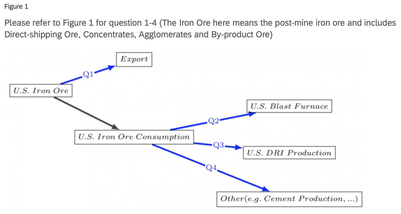
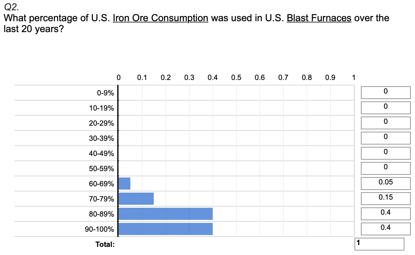
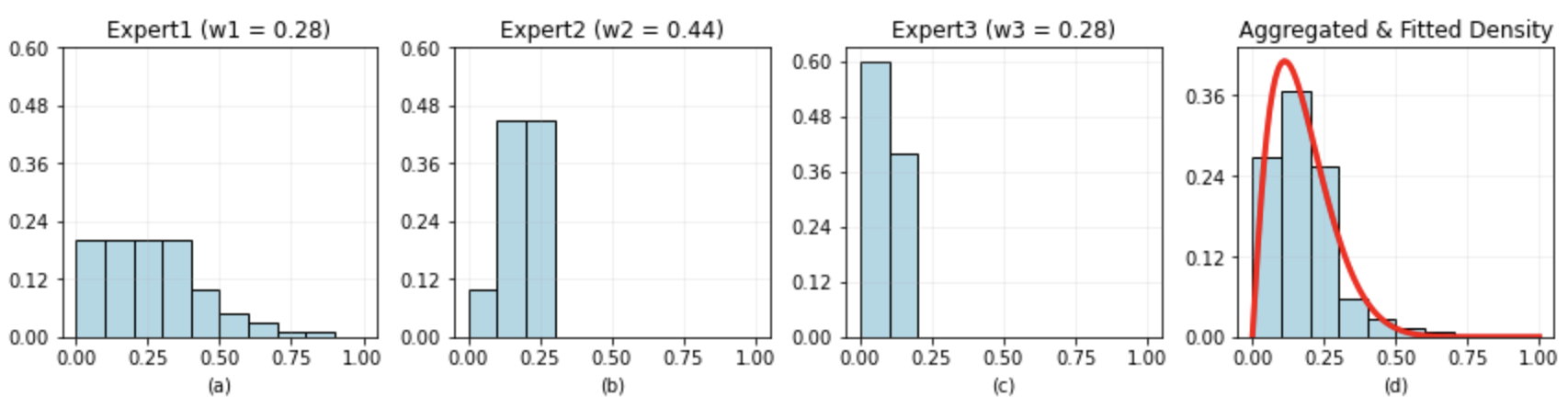
Figure 4: Prior elicitation required steel industry experts to complete an online Qualtrics Survey. The images above show an example question and expert response. The images below show an example calculation of an aggregated prior for the fraction of U.S. Iron Ore that is exported. Only 3 expert responses are shown for the sake of concision. Their weights have been normalized accordingly to sum to unity.

Linear pooling was used to aggregate the responses from the multiple experts into a single proper prior PDF for each MFA variable. First, weights were assigned to each of the experts based on their responses to 9 seeding questions using Cooke’s method. A wide range of expert weighting values were obtained with the most informed expert having a weight of 0.299 and the least informed expert having a weight of less than 0.001. Figure 4 shows how the response of multiple steel experts are combined to form a single aggregated prior PDF for an MFA variable.

3.2 Collecting MFA Data Records and Constructing the Prior for Data Noise Standard Deviation ($\sigma$)

After construction of the allocation fraction and external inflow priors, U.S. steel flow MFA data were collected. We focus here on 2012 data although any year from the previous 20 years could also have been chosen. The steel flow data were collected from the United States Geological Survey (USGS) [66, 67, 68], World Steel Association (WSA) [17] and Zhu et al. [11]. A complete record of all the collected MFA data is provided in SI Section 5.

The collected MFA data are published without accompanying uncertainty information while data error is inevitable. Subsequently, the noise for each piece of collected data is modeled as an independent relative error (see Eqn. 7) that follows a Gaussian distribution with zero mean and a standard deviation $\sigma$. Expert elicitation could be used to derive an informed prior for $\sigma$; e.g., experts could be interviewed on the likely accuracy of USGS and WSA data. In this study, however, the prior on $\sigma$ is instead modeled as only weakly informative using a normal distribution truncated below zero and above 0.5 with hyperparameters set such that $\mathbb{P}(\sigma\leq 0.1)$ and $\mathbb{P}(\sigma\leq 0.3)$ are approximately 0.5 and 0.95 respectively, maintaining a reasonable probability that the data can be of high quality.

3.3 Case Study Results: U.S. Steel flow in 2012

The Bayesian inference is implemented using SMC in PyMC3 with the code adapted from Lupton and Allwood [14]. It takes approximately 17 hours to generate 10,000 samples using an Intel(R) CoreTM i7-11800H CPU, 2.30 GHz. The prior and posterior results are shown in Fig. 5 and 6 respectively. The width of each line is proportional to the mean of the flow and the color indicates the uncertainty level, with a smaller relative uncertainty displayed in darker blue colors.

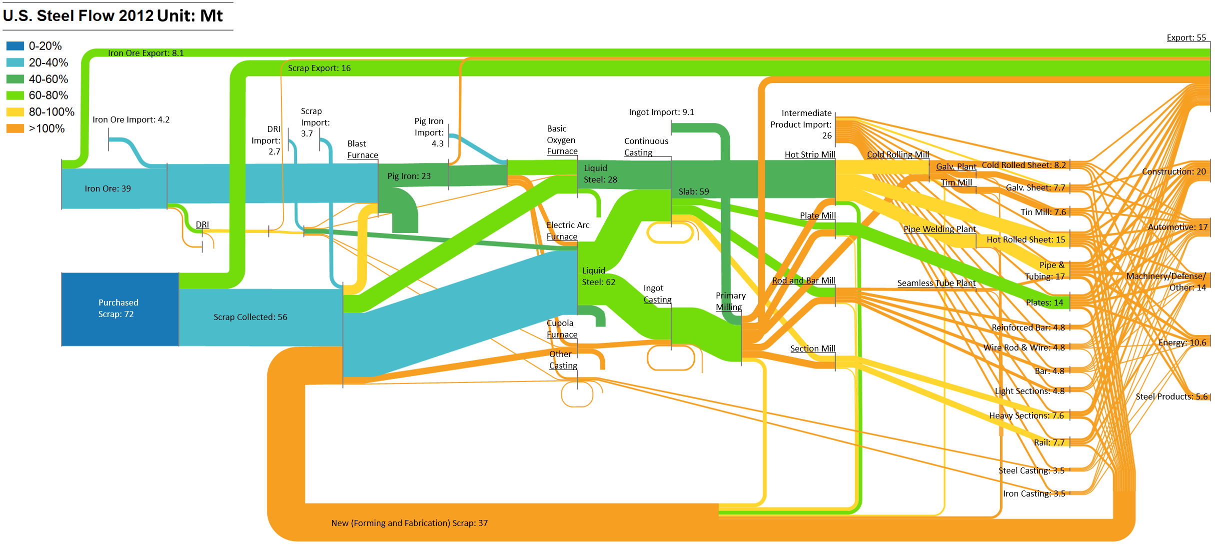
Figure 5: The prior for the U.S. Steel flow in 2012. All numbers on the flows refer to the mean of the prior mass flow in units of million metric tons (Mt). The uncertainty percentages refer to the flow standard deviation as a percentage of the flow mean. All mass flows refer to steel except for the iron ore flows that include the non-iron mass (e.g., oxygen and gangue).

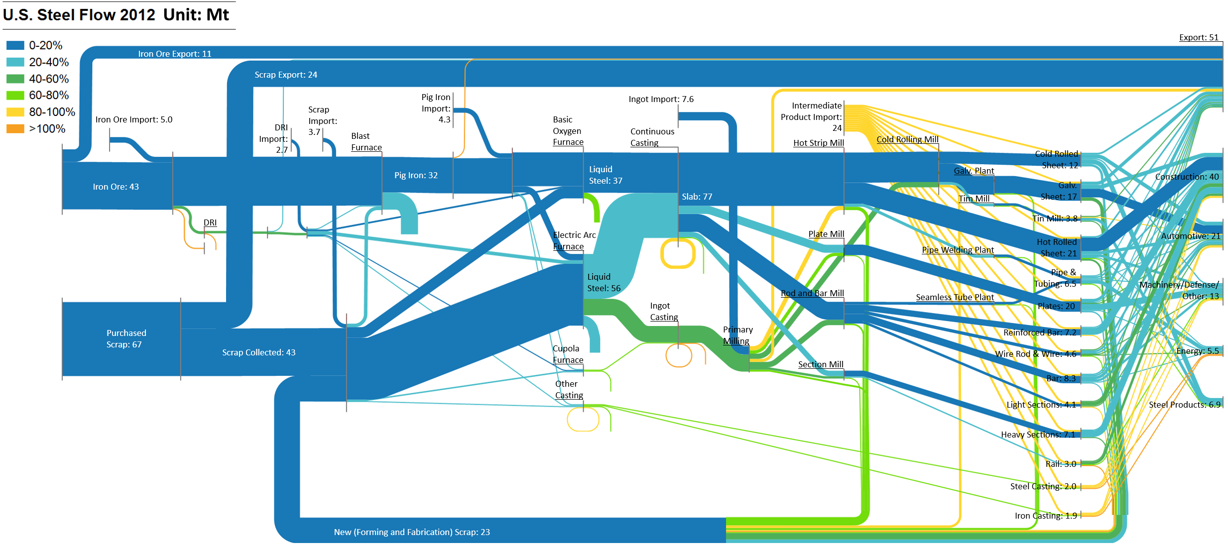
Figure 6: The posterior for the U.S. Steel flow in 2012. All numbers on the flows refer to the mean of the prior mass flow in units of million metric tons (Mt). The uncertainty percentages refer to the flow standard deviation as a percentage of the flow mean. All mass flows refer to steel except for the iron ore flows that include the non-iron mass (e.g., oxygen and gangue).

Figure 7 shows the prior and posterior distributions for $\phi$ and $\sigma$ associated with three prominent upstream flows. There is a significant uncertainty reduction for all $\phi$ shown in Fig. 7 (a)–(c). For example, despite a relatively flat prior for the fraction of (solid or liquid) pig iron consumed in the Basic Oxygen Furnace (BOF), even with only 1 year of data the posterior is able to reflect that pig iron is mainly consumed in the BOF. Figure 7 (d)–(f) presents the prior and posterior for $\sigma$. The posterior distribution for $\sigma$ on “Iron Ore $\rightarrow$ BF” is more concentrated than the prior, indicating that the data noise can be learned from data. However, in comparison to $\phi$, there is a lower uncertainty reduction in $\sigma$. In an effort to enhance data noise learning, we explored the use of multiple years of data to prompt a greater reduction in uncertainty.

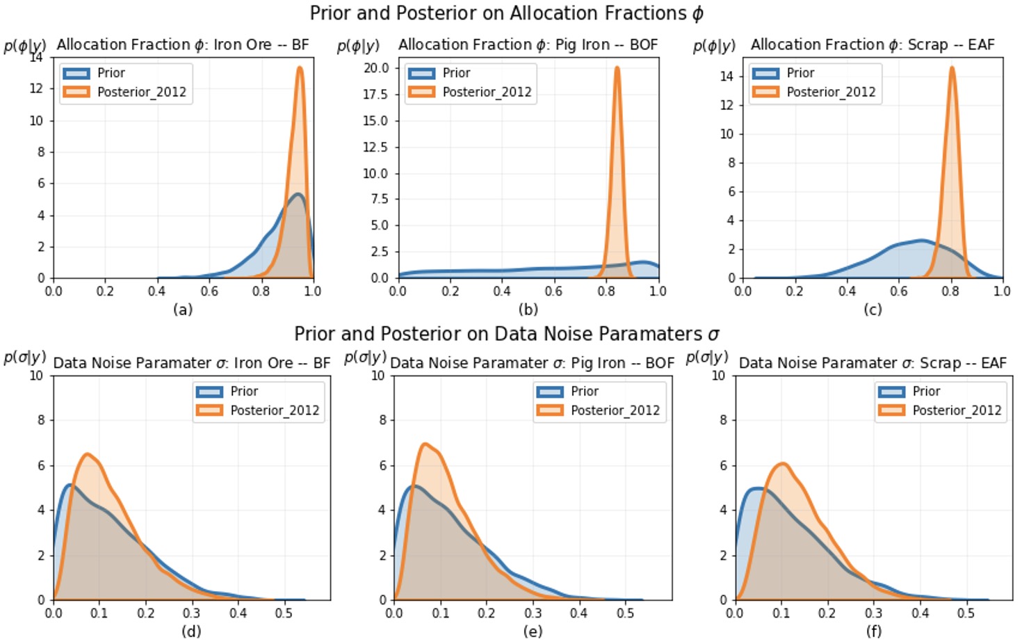
Figure 7: Examples of prior and posterior on Allocation Fractions ($\phi$) and Data Noise Parameters ($\sigma$) for Annual U.S. Steel Flow (2012).

3.4 Enhanced learning using data collected from multiple years

One interpretation of the modest residual uncertainty for $\sigma$ shown in Fig. 7 is that there is still a low amount of information from data for inference if using data only from 2012. However, some of the $\phi$ are very likely to be similar across years. In addition, the measurement noise $\epsilon$ in different years is also possibly a realization from a similar distribution. If the allocation fractions $\phi$ and data noise parameter $\sigma$ on regularly reported MFA data (e.g., the USGS data record on “Iron ore $\rightarrow$ BF”) can be verified to be similar across a multi-year time period, then there is the potential to leverage multiple years’ worth of MFA data to enhance the learning of the data noise. Therefore, we used Bayes factor analysis (see SI Section 3) to check and justify modeling the allocation fractions and data noise parameters as constant across five years worth of USGS and WSA data (2012–2016), allowing the inference to be rerun using these additional years’ data.

Figure 8 shows the posteriors on $\phi$ and $\sigma$ when utilizing one years (2012) versus five years worth (2012–2016) of data. Figure 8 shows a reduction in $\sigma$ uncertainty when leveraging these extra data. For “Iron ore $\rightarrow$ BF”, utilizing 2012–2016 data reduces both the uncertainty on $\sigma$ and its mean value. On the other hand, the posterior on “Pig Iron $\rightarrow$ BOF” shows a reduced uncertainty for $\sigma$ but an increase in its mean. This could be because the data noise is indeed low in the “Iron ore $\rightarrow$ BF” data and high in the “Pig Iron $\rightarrow$ BOF” data. However, readers should note that the data noise calculated here reflects not only the collected MFA data quality but also any inadequacy in the modeling; e.g., from the MFA network structure used to the assumption of constant data noise errors across the five years.

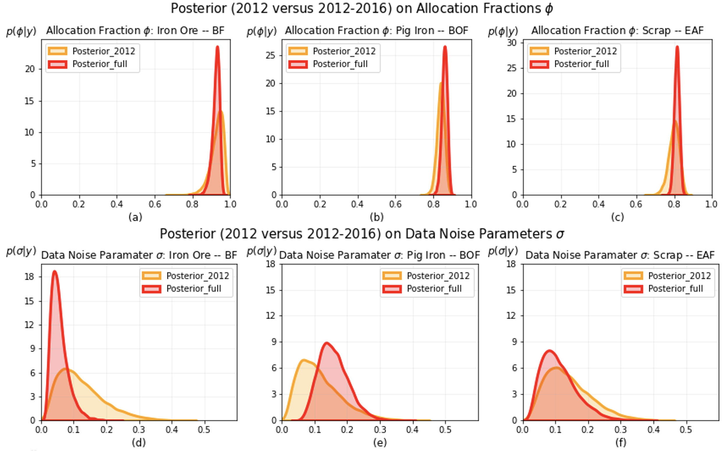
Figure 8: Examples of posteriors on Allocation Fractions ($\phi$) and Data Noise Parameters ($\sigma$) using data only from 2012 versus full data from 2012–2016.

4 Discussion and Conclusions

This paper has introduced, adapted, and demonstrated the use of expert elicitation techniques to define proper prior distributions for Bayesian inference in MFA, and illustrated how the noise level in collected MFA data may itself be learned from data. Below, we discuss the lessons learned from the case study on U.S. steel flows, limitations of these approaches, and future work to advance the Bayesian approach in MFA.

4.1 Using Expert Elicitation in MFA

Expert elicitation allows the use of informed priors in MFA and will result in a quick reduction in parametric uncertainties when combined with collected data. In cases where no or negligible MFA data can be collected, expert elicitation provides a statistically robust method of estimating material flows. Expert elicitation may also reveal model-form mistakes in the MFA structure that were not apparent beforehand.

A potential drawback is the time needed to find experts, develop well-posed elicitation questions, and process the responses. For the case study, the authors were concerned that each interview might take more than one hour and that there would be significant confusion regarding our request to answer questions with histograms and PDFs rather than point values. However, most interviews were completed within 30 minutes and the authors only received approximately one survey clarification question per expert. Even experts who were unaccustomed to PDFs were comfortable completing the questions after reviewing the example question and solution we posted at the start of the survey. There was one case where the sum of upper bound elicited allocation fractions from a single source node was less than unity. While this does not prevent hyper-parameter fitting to a Dirichlet PDF it does suggest that either the expert made a mistake or that the expert thought that the model structure was incorrect, believing that there should be another destination node from that source node. A more sophisticated elicitation procedure could ask experts to evaluate the probability of candidate MFA model structures in addition to MFA parametric values. Overall, the Fixed Interval Method used in the case study was found to be an effective and quick method of eliciting allocation fraction and external inflow priors.

In the case study, a single weight was assigned to each expert. A potential problem is that the expert might not be uniformly informed across the domain of interest; e.g., an expert might be an authority on steel recycling but relatively uninformed on primary steelmaking. In the case study, it was possibly a case of non-uniform expertise that affected the derivation of the aggregated prior for the allocation fraction from (liquid and solid) pig iron to the BOF. The expert who received the highest weighting gave an apparently erroneous answer to the elicitation question on “Pig Iron $\rightarrow$ BOF”, responding that less than 50% of the iron flows into the BOF. The high weighting given to this expert meant that the aggregated prior for Pig Iron to BOF was relatively uninformed (flat) despite the other seven experts responding that the majority of pig iron flows into the BOF (see Fig. 7). One option to avoid such problems would be to assign multiple weights to each expert corresponding to different areas of expertise; however, that would require the development and asking of more seeding questions tailored to those different areas of expertise.

A source of confusion for one of the experts was whether the survey was asking for uncertainty on a given variable (e.g., $\theta=\frac{\text{Amount of Iron Ore Exported}}{\text{Amount of Iron Ore Produced}}$) or its variability over space and time; e.g., the histogram of the $\frac{\text{Amount of Iron Ore Exported }}{\text{Amount of Iron Ore Produced}}$ for each month in a year or across regions. The survey was eliciting the former and we found it useful to clarify that we were seeking uncertainty rather than variability by demonstrating a “toy” example and also using equations to define the variable of interest.

4.2 Learning the MFA Variables and Data Noise Parameters

The uncertainty reduction in the U.S. steel mass flows between the prior and posterior is shown by the increase in dark blue colors between Fig. 5 and 6. The ability to quantify and reduce these uncertainties in a principled manner using Bayesian inference is appealing as it can lead to more informed decision- and policy-making. For example, the benefits of deploying a new, more energy efficient mill technology can be calculated with greater confidence for the cold rolling mill (calculated to have processed an expected 32.3 Mt in 2012 with a standard deviation of 3.27 Mt) compared to the primary mill (calculated to have processed a smaller expected value of 23.1 Mt in 2012 but with a larger standard deviation of 8.69 Mt).

A new MFA approach explored in this article has been to incorporate data noise parameters as random variables. The allocation fractions and the data noise parameters are then learned simultaneously with collected MFA data. Intuitively it is harder to achieve great uncertainty reductions using this method because the same amount of data is used to provide information on more parameters, even though it is a more honest representation if we do not know the true data noise. To combat this, we used Bayes factor analysis to verify the existence of time-invariant data noise parameters, allowing us to incorporate multiple years worth of data for greater uncertainty reductions.

As observed elsewhere [14], a potential drawback of the Bayesian approach to MFA is the computational cost of the Monte Carlo-based algorithms. Modeling the data noise parameters as random variables significantly increased the stochastic dimension of the problem and in turn computational cost, from 3 hours/run if the data noise parameters are prescribed as constants, to 17 hours/run when the data noise parameters are modeled as random variables. Therefore, there is a trade-off between the amount of bias and the computational cost. However, the computational speed can be increased by, for example, using multi-core processors to run algorithms that can be parallelized or applying approximate Bayesian techniques such as variational inference [69].

4.3 Future Work

The Bayesian approach to MFA provides a mathematically principled procedure to incorporate expert knowledge alongside sparse, noisy, and often incomplete data records: a data-informed model learning approach. We plan to investigate how this model-and-data relationship can be leveraged to create intelligent data acquisition strategies for seeking out the most informative data that can tell us what the MFA structure should look like, and what its parameters values are. These remain important challenges in MFA and can be approached by combining the use of Bayesian inference for uncertainty quantification early in the MFA exercise with the principles of Bayesian experimental design [70, 71].

5 Acknowledgements

The authors would like to thank all the steel experts interviewed for this study. This material is based upon work supported by the National Science Foundation under Grant No. #2040013.

6 Supporting Information

The Supporting Information (SI) includes data and literature reviews helpful to understanding the main article as well as links to elicitation surveys and Python Scripts that allow other MFA practitioners to use expert elicitation and data noise learning techniques.

References

- [1] Paul Brunner and Helmut Rechberger. Handbook of Material Flow Analysis: For Environmental, Resource, and Waste Engineers. CRC Press, Boca Raton, FL, 2016. doi:10.1201/9781315313450.
- [2] J.M. Cullen and D.R Cooper. Material flows and uncertainty. Annual Review of Materials Research, 2022. doi:https://doi.org/10.1146/annurev-matsci-070218-125903.
- [3] Thomas E. Graedel. Material Flow Analysis from Origin to Evolution. Environmental Science & Technology, 53(21):12188–12196, 2019. doi:10.1021/acs.est.9b03413.
- [4] Oliver Schwab and Helmut Rechberger. Information Content, Complexity, and Uncertainty in Material Flow Analysis. Journal of Industrial Ecology, 22(2):263–274, 2018. doi:10.1111/jiec.12572.
- [5] E. T. Jaynes. Probability Theory: The Logic of Science. Cambridge University Press, 2003. doi:10.1017/CBO9780511790423.
- [6] Introduction to Probability. Athena Scientific Optimization and Computation Series.
- [7] James O. Berger. Statistical Decision Theory and Bayesian Analysis. Springer Series in Statistics. Springer New York, New York, NY, 1985. doi:10.1007/978-1-4757-4286-2.
- [8] Udo Von Toussaint. Bayesian inference in physics. Reviews of Modern Physics, 83:943–999, 2011. doi:10.1103/RevModPhys.83.943.
- [9] Lemuel A. Moyé. Bayesians in clinical trials: Asleep at the switch. Statistics in Medicine, 27(4):469–482, 2008. doi:10.1002/sim.2928.
- [10] Grant M. Kopec, Julian M. Allwood, Jonathan M. Cullen, and Daniel Ralph. A General Nonlinear Least Squares Data Reconciliation and Estimation Method for Material Flow Analysis. Journal of Industrial Ecology, 20(5):1038–1049, 2016. doi:10.1111/jiec.12344.
- [11] Yongxian Zhu, Kyle Syndergaard, and Daniel R. Cooper. Mapping the Annual Flow of Steel in the United States. Environmental Science & Technology, 53(19):11260–11268, 2019. doi:10.1021/acs.est.9b01016.
- [12] D. Wang and J. A. Romagnoli. A Framework for Robust Data Reconciliation Based on a Generalized Objective Function. Industrial & Engineering Chemistry Research, 42(13):3075–3084, 2003. doi:10.1021/ie0206655.
- [13] Fadri Gottschalk, Roland W. Scholz, and Bernd Nowack. Probabilistic material flow modeling for assessing the environmental exposure to compounds: Methodology and an application to engineered nano-TiO2 particles. Environmental Modelling & Software, 25(3):320–332, 2010. doi:10.1016/j.envsoft.2009.08.011.
- [14] Richard C. Lupton and Julian M. Allwood. Incremental Material Flow Analysis with Bayesian Inference. Journal of Industrial Ecology, 22(6):1352–1364, 2018. doi:10.1111/jiec.12698.
- [15] Jonathan M. Cullen, Julian M. Allwood, and Margarita D. Bambach. Mapping the Global Flow of Steel: From Steelmaking to End-Use Goods. Environmental Science & Technology, 46(24):13048–13055, 2012. doi:10.1021/es302433p.
- [16] United Nations Comtrade Database. International trade statistics yearbook, 2012. https://comtrade.un.org/pb/downloads/2012/VolI2012.pdf.
- [17] World Steel. Steel statistical yearbook, 2012. https://worldsteel.org/wp-content/uploads/Steel-Statistical-Yearbook-2012.pdf.
- [18] Marie Bonnin, Catherine Azzaro-Pantel, Luc Pibouleau, Serge Domenech, and Jacques Villeneuve. Development and validation of a dynamic material flow analysis model for French copper cycle. Chemical Engineering Research and Design, 91(8):1390–1402, 2013.
- [19] Shannon M. Lloyd and Robert Ries. Characterizing, Propagating, and Analyzing Uncertainty in Life-Cycle Assessment: A Survey of Quantitative Approaches. Journal of Industrial Ecology, 11(1):161–179, 2007. doi:10.1162/jiec.2007.1136.
- [20] Do Nga, Trinh Anh Duc, and Nishida Kei. Modification of uncertainty analysis in adapted material flow analysis: Case study of nitrogen flows in the Day-Nhue River Basin, Vietnam. Resources, Conservation and Recycling, 88, 2014. doi:10.1016/j.resconrec.2014.04.006.
- [21] Fadri Gottschalk, Tobias Sonderer, Roland W. Scholz, and Bernd Nowack. Possibilities and limitations of modeling environmental exposure to engineered nanomaterials by probabilistic material flow analysis. Environmental Toxicology and Chemistry, 29(5):1036–1048, 2010. doi:10.1002/etc.135.
- [22] Robert L. Winkler. The Assessment of Prior Distributions in Bayesian Analysis. Journal of the American Statistical Association, 62(319):776–800, 1967. doi:10.1080/01621459.1967.10500894.
- [23] Danila Azzolina, Paola Berchialla, Dario Gregori, and Ileana Baldi. Prior Elicitation for Use in Clinical Trial Design and Analysis: A Literature Review. International Journal of Environmental Research and Public Health, 18(4), 2021. doi:10.3390/ijerph18041833.
- [24] A. V. Ramanan, L. V. Hampson, H Lythgoe, A. P. Jones, B Hardwick, H Hind, B Jacobs, D Vasileiou, I Wadsworth, N Ambrose, J Davidson, P. J. Ferguson, T Herlin, A Kavirayani, O. G. Killeen, S Compeyrot-Lacassagne, R. M. Laxer, M Roderick, J. F. Swart, C. M. Hedrich, and M. W. Beresford. Defining consensus opinion to develop randomised controlled trials in rare diseases using Bayesian design: An example of a proposed trial of adalimumab versus pamidronate for children with CNO/CRMO. PLOS ONE, 14:1–16, 2019. doi:10.1371/journal.pone.0215739.
- [25] Laura Bojke, Marta Soares, Karl Claxton, Abigail Colson, Aimée Fox, Christopher Jackson, Dina Jankovic, Alec Morton, Linda Sharples, and Andrea Taylor. Developing a reference protocol for structured expert elicitation in health-care decision-making: a mixed-methods study. Health Technology Assessment, 25:1–124, 2021. doi:10.3310/hta25370.
- [26] Ryan Wiser, Karen Jenni, Joachim Seel, Erin Baker, Maureen Hand, Eric Lantz, and Aaron Smith. Expert elicitation survey on future wind energy costs. Nature Energy, 1:16135, 2016. doi:10.1038/nenergy.2016.135.
- [27] Suraje Dessai, Ajay Bhave, Cathryn Birch, Declan Conway, Luis Garcia-Carreras, John Paul Gosling, Neha Mittal, and David Stainforth. Building narratives to characterise uncertainty in regional climate change through expert elicitation. Environmental Research Letters, 13(7):074005, 2018. doi:10.1088/1748-9326/aabcdd.
- [28] Agnes Montangero and Hasan Belevi. Assessing nutrient flows in septic tanks by eliciting expert judgement: A promising method in the context of developing countries. Water Research, 41(5):1052–1064, 2007. doi:10.1016/j.watres.2006.10.036.
- [29] Fabrice Mathieux and Daniel Brissaud. End-of-life product-specific material flow analysis. Application to aluminum coming from end-of-life commercial vehicles in Europe. Resources, Conservation and Recycling, 55(2):92–105, 2010. doi:10.1016/j.resconrec.2010.07.006.
- [30] Sindhu R. Johnson, George Tomlinson, Gillian A. Hawker, John T. Granton, and Brian M. Feldman. Methods to elicit beliefs for Bayesian priors: a systematic review. Journal of clinical epidemiology, 63 4:355–69, 2010.
- [31] Alireza Daneshkhah and Jeremy E. Oakley. Eliciting Multivariate Probability Distributions. In Klaus Böcker, editor, Rethinking Risk Measurement and Reporting, pages 179–204. Risk Books, London, United Kingdom, 2010. doi:10.4135/9788132114062.n2.
- [32] Anthony O’Hagan, Caitlin E. Buck, Alireza Daneshkhah, J. Richard Eiser, Paul H. Garthwaite, David J. Jenkinson, Jeremy E. Oakley, and Tim Rakow. Uncertain Judgements: Eliciting Experts’ Probabilities. John Wiley & Sons, Ltd, Chichester, UK, 2006. doi:10.1002/0470033312.
- [33] Jeremy E. Oakley. Eliciting Univariate Probability Distributions. In Klaus Böcker, editor, Rethinking Risk Measurement and Reporting, pages 155–178. Risk Books, London, United Kingdom, 2010. doi:10.1590/1806-9126-RBEF-2021-0424.
- [34] Allan H. Murphy and Robert L. Winkler. Credible Interval Temperature Forecasting: Some Experimental Results. Monthly Weather Review, 102(11):784–794, 1974. doi:10.1175/1520-0493(1974)102<0784:CITFSE>2.0.CO;2.
- [35] Paul H Garthwaite, Joseph B Kadane, and Anthony O’Hagan. Statistical methods for eliciting probability distributions. Journal of the American Statistical Association, 100(470):680–701, 2005. doi:10.1198/016214505000000105.
- [36] Anthony O’Hagan. Eliciting expert beliefs in substantial practical applications. The Statistician, 47:21–35, 1998.
- [37] Ali Abbas, David Budescu, Hsiu-Ting Yu, and Ryan Haggerty. A comparison of two probability encoding methods: Fixed probability vs. fixed variable values. Decision Analysis, 5:190–202, 2008. doi:10.1287/deca.1080.0126.
- [38] Daniel Gigone and Reid Hastie. The common knowledge effect: Information sharing and group judgment. Journal of Personality and Social Psychology, 65:959–974, 1993.
- [39] S Plous. The psychology of judgment and decision making. Mcgraw-Hill Book Company, 1993.
- [40] Janet A Sniezek. Groups under uncertainty: An examination of confidence in group decision making. Organizational Behavior and Human Decision Processes, 52(1):124–155, 1992. doi:10.1016/0749-5978(92)90048-C.
- [41] Garold Stasser and William Titus. Pooling of unshared information in group decision making: Biased information sampling during discussion. Journal of Personality and Social Psychology, 48:1467–1478, 1985.
- [42] Harold Linstone and Murray Turoff. The Delphi Method: Techniques and Applications. Murray Turoff and Harold A. Linstone, 2002.
- [43] Gene Rowe and George Wright. The Delphi technique as a forecasting tool: issues and analysis. International Journal of Forecasting, 15(4):353–375, 1999. doi:10.1016/S0169-2070(99)00018-7.
- [44] Morris H. Degroot. Reaching a Consensus. Journal of the American Statistical Association, 69(345):118–121, 1974. doi:10.1080/01621459.1974.10480137.
- [45] Andre Delbecq, Andrew Ven, and David Gustafson. Group Techniques for Program Planning: A Guide to Nominal Group and Delphi Processes. Green Briar Press, Middleton, WI, 1986.
- [46] Christian Genest and James V Zidek. Combining probability distributions: A critique and an annotated bibliography. Statistical Science, 1(1):114–135, 1986.
- [47] Robert T. Clemen and Robert L. Winkler. Combining probability distributions from experts in risk analysis. Risk Analysis, 19(2):187–203, 1999. doi:10.1111/j.1539-6924.1999.tb00399.x.
- [48] Roger M. Cooke, Susie ElSaadany, and Xinzheng Huang. On the performance of social network and likelihood-based expert weighting schemes. Reliability Engineering & System Safety, 93(5):745–756, 2008. doi:10.1016/j.ress.2007.03.017.
- [49] Willy Aspinall and Roger Cooke. Quantifying Scientific Uncertainty from Expert Judgement Elicitation. Risk and Uncertainty Assessment for Natural Hazards, pages 64–99, 2011. doi:10.1017/CBO9781139047562.005.
- [50] Abigail R Colson and Roger M Cooke. Expert Elicitation: Using the Classical Model to Validate Experts’ Judgments. Review of Environmental Economics and Policy, 12(1):113–132, 2018.
- [51] Roger M. Cooke. Experts in Uncertainty: Opinion and Subjective Probability in Science. Oxford, England: Oxford University Press, 1991.
- [52] Solomon Kullback. Information theory and statistics. Courier Corporation, 1997.
- [53] Justin Eggstaff, Thomas Mazzuchi, and Shahram Sarkani. The effect of the number of seed variables on the performance of Cooke’s classical model. Reliability Engineering & System Safety, 121:72–82, 01 2014. doi:10.1016/j.ress.2013.07.015.
- [54] Marissa McBride, Stephen Garnett, Judit Szabo, Allan Burbidge, Stuart Butchart, Les Christidis, Guy Dutson, Hugh Ford, Richard Loyn, David Watson, and Mark Burgman. Structured elicitation of expert judgments for threatened species assessment: A case study on a continental scale using email. Methods in Ecology and Evolution, 3:906–920, 2012. doi:10.1111/j.2041-210X.2012.00221.x.
- [55] R Core Team. R: A Language and Environment for Statistical Computing. R Foundation for Statistical Computing, Vienna, Austria, 2017. URL: https://www.R-project.org/.
- [56] Rita Zapata-Vázquez, Anthony O’Hagan, and Leonardo Bastos. Eliciting expert judgements about a set of proportions. Journal of Applied Statistics, 41, 2014. doi:10.1080/02664763.2014.898131.
- [57] Andrew Gelman, Frederic Bois, and Jiming Jiang. Physiological Pharmacokinetic Analysis Using Population Modeling and Informative Prior Distributions. Journal of the American Statistical Association, 91(436):1400–1412, 1996. doi:10.1080/01621459.1996.10476708.
- [58] Andrew Gelman. Prior distributions for variance parameters in hierarchical models (comment on article by Browne and Draper). Bayesian Analysis, 1(3):515–534, 2006. doi:10.1214/06-BA117A.
- [59] W. R. Gilks, S. Richardson, and D. J. Spiegelhalter. Markov Chain Monte Carlo in Practice. Chapman & Hall, New York, NY, 1996.
- [60] Christophe Andrieu, Nando de Freitas, Arnaud Doucet, and Michael I. Jordan. An Introduction to MCMC for Machine Learning. Machine Learning, 50:5–43, 2003. doi:10.1023/A:1020281327116.
- [61] Christian P. Robert and George Casella. Monte Carlo Statistical Methods. Springer New York, New York, NY, 2004. doi:10.1007/978-1-4757-4145-2.
- [62] Steve Brooks, Andrew Gelman, Galin Jones, and Xiao-Li Meng, editors. Handbook of Markov Chain Monte Carlo. Chapman & Hall/CRC, 2011. doi:10.1201/b10905.
- [63] Michael Betancourt. A Conceptual Introduction to Hamiltonian Monte Carlo, 2018. arXiv:1701.02434.
- [64] Samuel Livingstone, Michael Betancourt, Simon Byrne, and Mark Girolami. On the Geometric Ergodicity of Hamiltonian Monte Carlo, 2018. arXiv:1601.08057.
- [65] Arnaud Doucet, Nando de Freitas, and Neil Gordon. An introduction to sequential Monte Carlo methods. In Sequential Monte Carlo methods in practice, pages 3–14. Springer, 2001.
- [66] United States Geological Survey. Iron ore, 2012. https://s3-us-west-2.amazonaws.com/prd-wret/assets/palladium/production/mineral-pubs/iron-ore/myb1-2012-feore.pdf.
- [67] United States Geological Survey. Iron and steel, 2012. https://s3-us-west-2.amazonaws.com/prd-wret/assets/palladium/production/mineral-pubs/iron-steel/myb1-2012-feste.pdf.
- [68] United States Geological Survey. Iron and steel scrap, 2012. https://s3-us-west-2.amazonaws.com/prd-wret/assets/palladium/production/mineral-pubs/iron-steel-scrap/myb1-2012-fescr.pdf.
- [69] David M. Blei, Alp Kucukelbir, and Jon D. McAuliffe. Variational Inference: A Review for Statisticians. Journal of the American Statistical Association, 112(518):859–877, 2017. doi:10.1080/01621459.2017.1285773.
- [70] Kathryn Chaloner and Isabella Verdinelli. Bayesian Experimental Design: A Review. Statistical Science, 10(3):273–304, 1995. doi:10.1214/ss/1177009939.
- [71] Peter Müller. Simulation Based Optimal Design. Handbook of Statistics, 25:509–518, 2005. doi:10.1016/S0169-7161(05)25017-4.