Eyring-Kramers exit rates for the overdamped Langevin dynamics: the case with saddle points on the boundary

Abstract

Let $(X_{t})_{t\geq 0}$ be the stochastic process solution to the overdamped Langevin dynamics

$$dX_{t}=-\nabla f(X_{t})\,dt+\sqrt{h}\,dB_{t}$$

and let $\Omega\subset\mathbb{R}^{d}$ be the basin of attraction of a local minimum of $f:\mathbb{R}^{d}\to\mathbb{R}$. Up to a small perturbation of $\Omega$ to make it smooth, we prove that the exit rates of $(X_{t})_{t\geq 0}$ from $\Omega$ through each of the saddle points of $f$ on $\partial\Omega$ can be parametrized by the celebrated Eyring-Kramers laws, in the limit $h\to 0$. This result provides firm mathematical grounds to jump Markov models which are used to model the evolution of molecular systems, as well as to some numerical methods which use these underlying jump Markov models to efficiently sample metastable trajectories of the overdamped Langevin dynamics.

Keywords: Overdamped Langevin, Eyring-Kramers law, the exit problem, semi-classical analysis.

Motivation and statements of the main results

An informal presentation of the results

Let us first present in this section the motivation for this work, namely the modelling and the efficient simulation of metastable stochastic dynamics which are used in molecular dynamics, as well as an informal statement of the main results.

Overdamped Langevin dynamics and metastable exit. Let us consider a potential energy function

$$f:\mathbb{R}^{d}\to\mathbb{R},$$

which is assumed to be smooth and with non-degenerate critical points. A prototypical dynamics to describe the evolution of a molecular system in the energy landscape $f$ at a fixed temperature is the overdamped Langevin dynamics:

$$dX_{t}=-\nabla f(X_{t})\,dt+\sqrt{h}\,dB_{t},$$ (1)

where $(X_{t})_{t\geq 0}$ gives the positions of the atoms as a function of time, $h>0$ is (proportional to) the temperature, and $(B_{t})_{t\geq 0}$ is a $d$-dimensional standard Brownian motion. Let us consider $\Omega\subset\mathbb{R}^{d}$ a basin of attraction of a local minimum of $f$. In many cases of interest, the process spends a lot of time within $\Omega$ before leaving it, typically because the temperature $h$ is small compared to the energy barriers which have to be overcome to leave $\Omega$: this phenomenon is called metastability, and an exit which occurs after a long relaxation time within $\Omega$ is called a metastable exit (this will be formalized below using the notion of quasi-stationary distribution). We are interested in the so-called exit problem [33] which consists in precisely describing the exit event from $\Omega$ in such a situation, namely the law of the couple of random variables $(\tau,X_{\tau})$ where

$$\tau=\inf\{t\geq 0,\,X_{t}\notin\Omega\}$$ (2)

is the first exit time from $\Omega$, and $X_{\tau}$ is thus the first exit point. More precisely, we will show that for a metastable exit, in the limit $h\to 0$, the law of $(\tau,X_{\tau})$ can be approximated using a simple jump Markov model with exit rates from $\Omega$ parametrized by the celebrated Eyring-Kramers laws, a model which is sometimes called kinetic Monte Carlo in the physics literature [89]. These exit rates are associated with the local minima of $f$ on $\partial\Omega$, which are saddle points of $f$ (namely critical points of $f$ of index $1$) since $\Omega$ is a basin of attraction. These points are on the most probable exit pathways from $\Omega$.

Before providing more details on this kinetic Monte Carlo model in the next paragraph, let us emphasize that this question is both important in terms of modelling, and in terms of numerical simulation of (1). In terms of modelling, it gives a rigorous framework to prove that a coarse-grained version of the overdamped Langevin dynamics is indeed the kinetic Monte Carlo dynamics (a.k.a. Markov State Model) parametrized by Eyring-Kramers laws. Actually, if the states form a partition of $\mathbb{R}^{d}$ (which is indeed the case, up to a null set, if one defines the states as the basin of attractions of the local minima of $f$) and if all the exits are assumed to be metastable, one can even use a kinetic Monte Carlo model not only to sample the exit from a metastable state, but to actually describe the full evolution of the system, see for example [13, 77, 78, 89, 90, 74]. In tems of numerical simulations, metastability implies that the direct numerical simulation of (1) is prohibitive, because a lot of computational time is wasted in metastable states: using the simpler underlying kinetic Monte Carlo model, one can then accelerate the sampling of the exit event when the process $(X_{t})_{t\geq 0}$ remains trapped in a metastable state. This is the cornerstone of the so-called accelerated dynamics algorithms such as temperature accelerated dynamics [81] or hyperdynamics [88, 86], see [25] for more details. These algorithms are widely used in practice with applications in material science, see for instance [2, 71, 82, 32]. In this context, the states are very often defined as basins of attractions of local minima of $f$: this is indeed numerically convenient since a simple steepest decent algorithm can be used to identify in which state the system is.

Kinetic Monte Carlo and Eyring Kramers law. Let us recall that $\Omega$ is a basin of attraction of a local minimum of $f$. Thus, $f$ contains a unique critical point in $\Omega$, which is also the global minimum of $f$ in $\Omega$, denoted by $x_{0}$. Moreover, the local minima of $f$ on $\partial\Omega$ are saddle points of $f$, that we denote by $\{z_{1},\ldots,z_{n}\}\subset\partial\Omega$. The kinetic Monte Carlo algorithm models the exit event from $\Omega$ through a couple of random variables $(\tau_{\mathsf{kMC}},\mathsf{Y}_{\mathsf{kMC}})$, where $\tau_{\mathsf{kMC}}$ is the exit time and $\mathsf{Y}_{\mathsf{kMC}}\in\{z_{1},\ldots,z_{n}\}$ is equal to $z_{i}$ if the process exits $\Omega$ through a neighborhood of $z_{i}$ in $\partial\Omega$. The law of $(\tau_{\mathsf{kMC}},\mathsf{Y}_{\mathsf{kMC}})$ requires a collection of rates $(\mathsf{k}_{z})_{z\in\{z_{1},\ldots,z_{n}\}}$ associated with the saddle points, and is defined by the following three properties: (i) the time $\tau_{\mathsf{kMC}}$ is exponentially distributed with parameter $\sum_{z\in\{z_{1},\ldots,z_{n}\}}\mathsf{k}_{z}$

$$\tau_{\mathsf{kMC}}\sim\mathcal{E}\Big{(}\sum_{z\in\{z_{1},\ldots,z_{n}\}}\mathsf{k}_{z}\Big{)};$$ (3)

(ii) $\tau_{\mathsf{kMC}}$ is independent of $\mathsf{Y}_{\mathsf{kMC}}$ ; and (iii) for all $z\in\{z_{1},\ldots z_{n}\}$,

$$\mathbb{P}[\mathsf{Y}_{\mathsf{kMC}}=z]=\frac{\mathsf{k}_{z}}{\sum_{z\in\{z_{1},\ldots,z_{n}\}}\mathsf{k}_{z}}.$$ (4)

Moreover, in the setting of the so-called harmonic transition state theory, the rates are defined using the famous Eyring-Kramers formula [37, 89]: for any $z\in\{z_{1},\ldots,z_{n}\}$,

$$\mathsf{k}_{z}=\mathsf{P}_{z}\,e^{-\frac{2}{h}(f(z)-f(x_{0}))},$$ (5)

where, we recall, $x_{0}\in\Omega$ is the global minimum of $f$ in $\Omega$ and the prefactor $\mathsf{P}_{z}$ is

$$\mathsf{P}_{z}=\frac{|\mu_{z}|}{\pi}\frac{\sqrt{{\rm det\,Hess}\,f(x_{0})}}{\sqrt{|{\rm det\,Hess}\,f(z)|}},$$ (6)

where $\mu_{z}$ is the negative eigenvalue of $\operatorname{Hess}f(z)$.

Remark 1.

The Eyring-Kramers formulas are sometimes defined with a prefactor which is the half of the right-hand-side in (6). This depends whether one considers exit rates (as in this work) or transition rates (as for example in the works [9, 10] where eigenvalues of the infinitesimal generator of the process $(X_{t})_{t\geq 0}$ are identified with transition rates). The transition rates are half of the exit rates since once the process reaches a saddle point $z$, it has a probability $1/2$ to immediately come back to $\Omega$, and a probability $1/2$ to actually transition to the neighbooring state (see e.g. [61, Remark 8] for further discussions).

The objective of this work is to show that, for a metastable exit, in the limit $h\to 0$, the law of $(\tau_{\mathsf{kMC}},\mathsf{Y}_{\mathsf{kMC}})$ indeed approximates the law of $(\tau,X_{\tau})$, in a sense that will be made precise in the next paragraph. We will use the quasi-stationary distribution approach to metastability, which appears to be very useful to study the exit problem [55, 26, 6].

The quasi-stationary distribution approach to metastability. As explained above, we will study metastable exits, namely exits which occur after the stochastic process $(X_{t})_{t\geq 0}$ solution to (1) relaxes within $\Omega$. The notion of quasi-stationary distribution gives a way to formalize mathematically this idea. Let us recall standard facts on the existence and uniqueness of a quasi-stationary distribution for a diffusion process (see for example [14, 17] for more details).

Definition 2.

Let us denote by $\mathcal{P}(\Omega)$ the set of probability measures supported in $\Omega$. A quasi-stationary distribution in $\Omega\subset\mathbb{R}^{d}$ for a Markov process $(X_{t})_{t\geq 0}$ with values in $\mathbb{R}^{d}$ is a probability measure $\mu\in\mathcal{P}(\Omega)$ such that:

$$\forall t\geq 0,\forall\text{ measurable }A\subset\Omega,\quad\mu(A)=\frac{\mathbb{P}_{\mu}\left[X_{t}\in A,t<\tau\right]}{\mathbb{P}_{\mu}\left[t<\tau\right]},$$

where $\tau=\inf\{t>0,\,X_{t}\not\in\Omega\}$, and the subscript $\mu$ in $\mathbb{P}_{\mu}$ indicates that $X_{0}\sim\mu$.

It is well-known (see for example [55, 15]) that for a smooth potential $f$ and a bounded smooth domain $\Omega$, the process $(X_{t})_{t\geq 0}$ soution to (1) admits a unique quasi-stationary distribution on $\Omega$, denoted by $\nu_{h}$ in the following. Moroever, the previously cited works also show the following exponential convergence result: $\exists c>0,\forall\mu\in\mathcal{P}(\Omega),\exists C(\mu)>0,\exists t(\mu)>0$,

$$\forall t\geq t(\mu),\forall\text{ measurable }A\subset\Omega,\quad\big{|}\mathbb{P}_{\mu}\big{[}X_{t}\in A\big{|}t<\tau\big{]}-\nu_{h}(A)\big{|}\leq C(\mu)e^{-ct}.$$ (7)

Therefore, if the process $(X_{t})_{t\geq 0}$ remains trapped in $\Omega$ for a long-time, then $X_{t}$ is approximately distributed according to the quasi-stationary distribution $\nu_{h}$, which can thus be seen as a local equillibrium within $\Omega$. A metastable exit is then an exit which occurs after this local equilibrium has been reached, namely (using the Markov property) an exit for the process $(X_{t})_{t\geq 0}$ with initial condition $X_{0}\sim\nu_{h}$.

If $X_{0}\sim\nu_{h}$, the exit event satisfies the two fundamental properties (see for example [55, Proposition 2.4]):

$$\tau\sim\mathcal{E}(\lambda_{h})\text{ and }\tau\text{ is independent of }X_{\tau}.$$ (8)

With these two properties, one can use a kinetic Monte Carlo model to exactly sample the exit event. Indeed, assume again for simplicity that $\Omega$ is the basin of attraction of a local minimum of $f$, and let us denote by $\mathsf{W}_{+}^{z}\subset\partial\Omega$ the stable manifold of the saddle point $z\in\{z_{1},\dots,z_{n}\}$ (see (13) below for a precise definition). Up to a null set, the sets $(W_{+}^{z})_{z\in\{z_{1},\ldots,z_{n}\}}$ form a partition of the boundary $\partial\Omega$ of the basin of attraction. Let us now introduce the rates: for any $z\in\{z_{1},\ldots,z_{n}\}$,

$$\mathsf{k}_{z}^{o\ell}:=\frac{\mathbb{P}_{\nu_{h}}\big{[}X_{\tau}\in W^{+}_{z}\big{]}}{\mathbb{E}_{\nu_{h}}\big{[}\tau\big{]}}.$$ (9)

where the superscript $o\ell$ indicates that we consider the overdamped Langevin dynamics (1). Then the kinetic Monte Carlo model parametrized with these rates generate an exit event $(\tau_{\mathsf{kMC}},\mathsf{Y}_{\mathsf{kMC}})$ which is exactly consistent with the exit event $(\tau,X_{\tau})$ of the original dynamics (1). Indeed, using (3)–(4) and (8), one has: (i) $\tau_{\mathsf{kMC}}$ has the same law as $\tau$, (ii) $\tau_{\mathsf{kMC}}$ and $\mathsf{Y}_{\mathsf{kMC}}$ are independent, which is also the case for $\tau$ and $X_{\tau}$, and finally (iii) $\mathbb{P}(Y_{\mathsf{kMC}}=z)=\mathbb{P}(X_{\tau}\in W^{+}_{z})$. The mathematical question, which is the focus of this work, is now to prove that the rates $\mathsf{k}_{z}^{o\ell}$ can indeed be accurately approximated by the Eyring-Kramers formulas (5).

As already mentioned above (see footnote 1 and Remark 5 below), we will need to assume that $\Omega$ is smooth and bounded. The smoothness assumption may require to slightly modify the basin of attraction in the neighborhoods of the boundaries of $W^{+}_{z}$ where $\partial\Omega$ is not necessarily smooth (these are anyway typically high energy points which are thus visited with an exponentially small probability when $h\to 0$). Therefore, we will not consider exactly $\mathsf{k}_{z}^{o\ell}$ but the following rates: for any $z\in\{z_{1},\ldots,z_{n}\}$,

$$\mathsf{k}_{z}^{o\ell}(\Sigma_{z}):=\frac{\mathbb{P}_{\nu_{h}}\big{[}X_{\tau}\in\Sigma_{z}\big{]}}{\mathbb{E}_{\nu_{h}}\big{[}\tau\big{]}},$$ (10)

where $\Sigma_{z}$ is an open neighborhood of $z$ in $\partial\Omega$ which is positively stable for the gradient dynamics $\dot{x}=-\nabla f(x)$ and can be chosen arbitrarily large in $\partial\Omega\cap W^{+}_{z}$. We will prove that, under some geometric assumptions, these rates can indeed be accurately approximated by the Eyring-Kramers formulas in the small temperature regime $h\to 0$, see Corollary 8 below. This requires sharp estimates of the probabilities that $(X_{t})_{t\geq 0}$ exits $\Omega$ through the neighborhoods $\Sigma_{z}$ of the saddle points $z\in\{z_{1},\ldots,z_{n}\}$. These precise approximations of the exit rates are used in particular in the temperature accelerated dynamics algorithm [81] to extrapolate exit events observed at high temperature to low temperature (see Remark 9 for a discussion underlying the similarities between our mathematical analysis and this algorithm). Let us now leave this informal presentation and present the precise setting and the main mathematical results of this work.

Mathematical setting and statements of the main results

Notation and definition

In the following, $\Omega$ is a smooth bounded domain of $\mathbb{R}^{d}$. The function $f:\overline{\Omega}\to\mathbb{R}$ is assumed to be a $\mathcal{C}^{\infty}$ function, i.e. it is the restriction to $\overline{\Omega}$ of a smooth function defined on $\mathbb{R}^{d}$. We still denote by $f$ a smooth extension of $f:\overline{\Omega}\to\mathbb{R}$ to $\mathbb{R}^{d}$. Since the quantities of interest in this work only depends on the values of $f$ in the bounded set $\overline{\Omega}$, we assume throughout this work without loss of generality that the extension of $f$ is such that:

$$\sup_{x\in\mathbb{R}^{d}}|\nabla f(x)|+\sup_{x\in\mathbb{R}^{d}}|\text{Hess }f(x)|<+\infty,$$ (11)

where $\operatorname{Hess}f(x)$ denotes the Hessian matrix of $f$ at $x\in\mathbb{R}^{d}$.

Basic notation. The open ball of radius $r>0$ centred at $x\in\mathbb{R}^{d}$ is denoted by $\mathsf{B}(x,r)$. The unit outward normal to $\Omega$ at $z\in\partial\Omega$ is denoted by $\mathsf{n}_{\Omega}(z)$. The normal derivative on $\partial\Omega$ of a smooth function $f:\overline{\Omega}\to\mathbb{R}$ is denoted by $\partial_{\mathsf{n}_{\Omega}}f$. Its tangental gradient on $\partial\Omega$ is denoted by $\nabla_{\mathbf{T}}f$. We will simply write $\{f<a\}$ for the set $\{x\in\overline{\Omega},f(x)<a\}$.

Index of a critical point. A point $x\in\overline{\Omega}$ is a critical point of $f$ if $|\nabla f(x)|=0$. The critical point $x$ is non-degenerate if furthermore $\operatorname{Hess}f(x)$ is invertible. The function $f$ is a Morse function if all its critical points in $\overline{\Omega}$ are non degenerate. The non-degenerate critical point $x$ is of index $p\in\{0,\ldots,d\}$ if $\operatorname{Hess}f(x)$ admits $p$ negative eigenvalues. A saddle point is a non degenerate critical point with index 1. Notice that the index of a critical point on $\partial\Omega$ does not depend on the extension of $f$ outside $\overline{\Omega}$.

Stable and unstable manifolds. Let $x\in\mathbb{R}^{d}$ and denote by $\varphi_{x}(t)$ the maximal solution to the ordinary differential equation (which is defined for all $t\in\mathbb{R}$ by (11)):

$$\frac{d}{dt}\varphi_{x}(t)=-\nabla f(\varphi_{x}(t))\text{ with }\varphi_{x}(0)=x.$$ (12)

When $z\in\mathbb{R}^{d}$ is a saddle point of $f$, we denote by $\mathsf{W}_{+}^{z}$ and $\mathsf{W}_{-}^{z}$ respectively the stable and unstable manifolds of $z$ for the dynamics (12), i.e.

$$\mathsf{W}_{\pm}^{z}=\Big{\{}x\in\mathbb{R}^{d},\,\lim_{t\to\pm\infty}\varphi_{x}(t)=z\Big{\}}.$$ (13)

Let us recall the stable manifold theorem (see [50, Corollary 6.4.1]).

Theorem (Stable Manifold Theorem).

Let $f:\mathbb{R}^{d}\to\mathbb{R}$ satisfying (11), and let $z$ be a saddle point of $f$. Then, $\mathsf{W}_{+}^{z}$ and $\mathsf{W}_{-}^{z}$ are $\mathcal{C}^{\infty}$ embedded manifolds, with dimensions $d-1$ and $1$ respectively. Moreover, the tangent spaces of $\mathsf{W}_{+}^{z}$ and $\mathsf{W}_{-}^{z}$ at point $z$ satisfy

$$T_{z}\mathsf{W}_{+}^{z}={\rm Span}(\mathsf{e}_{1}\ldots,\mathsf{e}_{d-1})\text{ and }T_{z}\mathsf{W}_{-}^{z}={\rm Span}(\mathsf{e}_{d}),$$

where $(\mathsf{e}_{1},\ldots,\mathsf{e}_{d-1})$ is a basis of eigenvectors associated with the $d-1$ positive eigenvalues of $\operatorname{Hess}f(z)$ and $\mathsf{e}_{d}$ is an eigenvector associated with the negative eigenvalue of $\operatorname{Hess}f(z)$.

Agmon distance. Let us introduce the Agmon distance on $\overline{\Omega}$ which will be used to state our main results below.

Definition 3.

Let $f:\overline{\Omega}\to\mathbb{R}$ be a $\mathcal{C}^{\infty}$ function. The Agmon pseudo-distance between two points $x\in\overline{\Omega}$ and $y\in\overline{\Omega}$ is defined by:

$$\mathsf{d}_{a}\left(x,y\right)=\inf_{\gamma\in\mathcal{C}^{1}(x,y)}\int_{0}^{1}|\nabla f|(\gamma(t))\left|\gamma^{\prime}(t)\right|dt,$$

where $\mathcal{C}^{1}\left(x,y\right)$ is the set of curve $\gamma:[0,1]\to\overline{\Omega}$ which are $\mathcal{C}^{1}$ with $\gamma(0)=x$, $\gamma(1)=y$.

Since $f$ has a finite number of critical points in $\overline{\Omega}$ (which is indeed the case if $f$ is a Morse function on $\overline{\Omega}$), $\mathsf{d}_{a}$ is a distance since for all $x,y\in\overline{\Omega}$, $\mathsf{d}_{a}(x,y)=0$ if and only if $x=y$.

Assumptions

Let us now gather in the following assumption all the geometric requirements on $\Omega$ and $f$.

Assumption ($\Omega$-$f$).

The set $\Omega$ is a $\mathcal{C}^{\infty}$ bounded domain of $\mathbb{R}^{d}$. The functions $f:\overline{\Omega}\to\mathbb{R}$ and $f|_{\partial\Omega}$ are $\mathcal{C}^{\infty}$ Morse functions. Moreover:

1. The domain $\Omega$ is positively stable for (12): $\forall x\in\Omega,\,\forall t\geq 0,\,\varphi_{x}(t)\in\Omega$. Moreover, there exists $x_{0}\in\Omega$ such that for all $x\in\Omega$, $\lim_{t\to+\infty}\varphi_{x}(t)=x_{0}$.

2. For any critical point $z\in\partial\Omega$ of $f$, there exists an open subset $\Gamma_{z}$ of $\partial\Omega$ containing $z$ and satisfying the following:

   • If $z$ is a saddle point of $f$, then

     $$\overline{\Gamma_{z}}\subset\mathsf{W}_{+}^{z},$$ (14)

     and $\Gamma_{z}$ is positively stable for the dynamics (12): $\forall x\in\Gamma_{z},\forall t\geq 0,\,\varphi_{x}(t)\in\Gamma_{z}$.

   • If $z$ is not a saddle point of $f$, then $\partial_{\mathsf{n}_{\Omega}}f=0$ on $\Gamma_{z}$.

3. All the local minima of $f|_{\partial\Omega}$ are saddle points of $f$.

Assumption ($\Omega$-$f$) has simple consequences that will be used many times in the following (the proofs are standard, and provided in Section A.1 for completeness).

Lemma 4.

The following holds:

1. Assume that item 1 in ($\Omega$-$f$) is satisfied. Then $\partial_{\mathsf{n}_{\Omega}}f\geq 0$ on $\partial\Omega$ and $x_{0}$ is the only critical point of the function $f$ in $\Omega$. There is no local minimum of $f$ on $\partial\Omega$. Furthermore, $f(x_{0})=\min_{\overline{\Omega}}f<\min_{\partial\Omega}f$, $\{f<\min_{\partial\Omega}f\}$ is connected and $\partial\{f<\min_{\partial\Omega}f\}\cap\partial\Omega=\operatorname*{arg\,min}_{\partial\Omega}f$.

2. Assume that ($\Omega$-$f$) is satisfied. For all $z\in\partial\Omega$ such that $|\nabla f|(z)=0$, $\mathsf{n}_{\Omega}(z)$ is an eigenvector of $\operatorname{Hess}f(z)$ associated with a negative eigenvalue.

Other simple consequences of Assumption ($\Omega$-$f$) are the following. If $z\neq x$ are saddle points of $f$, then $\Gamma_{z}\cap\Gamma_{x}=\emptyset$. For $z$ a saddle point of $f$, the existence of a set $\Gamma_{z}$ whose closure is arbitrarily large in $\mathsf{W}_{+}^{z}$ and which is positively stable for the dynamics (12) is ensured by [26, Proposition 80], and $\Omega$ can then be defined such that $\Gamma_{z}\subset\partial\Omega$, see Remark 5. If $z$ is a saddle point of $f$ one can check that $\partial_{\mathsf{n}_{\Omega}}f=0\text{ on }\Gamma_{z}$ (since $\overline{\Gamma_{z}}\subset\mathsf{W}_{+}^{z}\cap\partial\Omega$). Finally, all the saddle points of $f$ in $\overline{\Omega}$ necessarily belong to $\partial\Omega$, and coincide with the local minima of $f$ on $\partial\Omega$.

Remark 5.

Let $\mathcal{A}(x_{0})$ be the basin of attraction of $x_{0}$ for the dynamics (12). As explained in the introduction, practitioners typically use as a definition of a bounded metastable domain the whole basin of attraction $\mathcal{A}(x_{0})$, which indeed naturally satisfies all the Assumptions ($\Omega$-$f$), except in some cases the smoothness assumption ($\Omega$ is indeed assumed to be $\mathcal{C}^{\infty}$ in ($\Omega$-$f$)). More precisley, $\partial\mathcal{A}(x_{0})$ is smooth on $\mathsf{W}_{+}^{z}$ for all $z\in\{z_{1},\ldots,z_{n}\}$, $\partial\mathcal{A}(x_{0})=\cup_{z\in\{z_{1},\ldots,z_{n}\}}\overline{\mathsf{W}_{+}^{z}}$ (see [67, Theorem B.13]), but singularities may occur on the boundaries of $\mathsf{W}_{+}^{z}$. In such a case, a domain $\Omega\subset\mathcal{A}(x_{0})$ satisfying ($\Omega$-$f$) can typically be obtained from $\mathcal{A}(x_{0})$ by slightly modifying it in neighborhoods of the points of the boundary $\partial\mathcal{A}(x_{0})$ where $\partial\mathcal{A}(x_{0})$ is not smooth, see for example Figure 1 for a schematic illustration in dimension 2. This modification typically only concerns high energy points, which are anyway visited with an exponentially small probability by the dynamics (1) in the regime $h\to 0$.

Figure 1: The basin of attraction $\mathcal{A}(0)=(-1,1)^{2}$ (for the dynamics (12)) of the local minimum $0\in\mathbb{R}^{2}$ of the Morse function $f(x,y)=-\cos(\pi x)-\cos(\pi y)$. There are 8 critical points on $\partial\mathcal{A}(0)$: four saddle points ($z_{1},z_{2},z_{3},z_{4}$) and four local maxima ($m_{1},m_{2},m_{3},m_{4}$). Each edge of the square $(-1,1)^{2}$ is the stable manifold of the saddle point it contains. In thick lines, a domain $\Omega$ satisfying ($\Omega$-$f$). In dashed lines, the level sets of $f$.

Definition 6.

When ($\Omega$-$f$) holds, the saddle points of $f$ in $\overline{\Omega}$ are denoted by $\{z_{1},\ldots,z_{n}\}\subset\partial\Omega$ and ordered such that

$$\min_{\partial\Omega}f=f(z_{1})=\ldots=f(z_{n_{0}})<f(z_{n_{0}+1})\leq\ldots\leq f(z_{n}).$$ (15)

The cardinal of $\arg\min f|_{\partial\Omega}$ is thus $n_{0}\in\{1,\ldots,n\}$. For all $k\in\left\{1,\ldots,n\right\}$, $\mu_{z_{k}}$ is the negative eigenvalue of ${\rm Hess}f(z_{k})$. For all $k\in\left\{1,\ldots,n\right\}$, we denote by $\Sigma_{z_{k}}\subset\partial\Omega$ an open set such that

$$z_{k}\in\Sigma_{z_{k}}\ \text{ and }\ \overline{\Sigma_{z_{k}}}\subset\Gamma_{z_{k}}.$$ (16)

A schematic representation of $\Omega$, $x_{0}$, $\{z_{1},\ldots,z_{n}\}$, and $\{\Sigma_{z_{1}},\ldots,\Sigma_{z_{n}}\}$ is given in Figure 2 when $n=4$.

From probability to partial differential equations

In order to give sharp asymptotic estimates of the rates (10) when $h\to 0$, we will rewrite the law of the random variable $(\tau,X_{\tau})$ using the first eigenvalue and eigenvector of the infinitesimal generator of the process (1) with homogeneous Dirichlet boundary conditions on $\Omega$. The small temperature regime then consists in analyzing the semi-classical limit of this eigenstate.

Let us denote by

$$\mathsf{L}_{f,h}^{(0)}=-\frac{h}{2}\Delta+\nabla f\cdot\nabla$$ (17)

the opposite of the infinitesimal generator of the process (1). Let $H^{1}_{0}(\Omega,e^{-\frac{2}{h}f}dx)$ be the set of functions $g\in H^{1}(\Omega,e^{-\frac{2}{h}f}dx)$ such that $g=0$ on $\partial\Omega$. The operator $\mathsf{L}_{f,h}^{(0)}$ on $L^{2}(\Omega,e^{-\frac{2}{h}f}dx)$ with domain

$$H^{2}(\Omega,e^{-\frac{2}{h}f}dx)\cap H^{1}_{0}(\Omega,e^{-\frac{2}{h}f}dx)=\big{\{}w\in H^{2}(\Omega,e^{-\frac{2}{h}f}dx),\,w=0\text{ on }\partial\Omega\big{\}}.$$

is denoted by $\mathsf{L}^{\mathsf{Di},(0)}_{f,h}(\Omega)$. The superscripts $\mathsf{Di}$ and $(0)$ respectively indicate that the operator is supplemented with Dirichlet boundary conditions, and acts on functions, namely $0$-forms (operators on $1$-forms will be also considered, see Section 2.5). The operator $\mathsf{L}^{\mathsf{Di},(0)}_{f,h}(\Omega)$ is the Friedrichs extension (see for instance [40, Section 4.3]) on $L^{2}(\Omega,e^{-\frac{2}{h}f}dx)$ of the closed quadratic form

$$\psi\in H^{1}_{0}(\Omega,e^{-\frac{2}{h}f}dx)\mapsto\frac{h}{2}\int_{\Omega}|\nabla\psi|^{2}\,e^{-\frac{2}{h}f}.$$ (18)

The operator $\mathsf{L}^{\mathsf{Di},(0)}_{f,h}(\Omega)$ is thus a positive self-adjoint operator on $L^{2}(\Omega,e^{-\frac{2}{h}f}dx)$. In addition, it has a compact resolvent (from the compact injection $H^{1}_{0}(\Omega,e^{-\frac{2}{h}f}dx)\subset L^{2}(\Omega,e^{-\frac{2}{h}f}dx)$). Then, by standard results on elliptic operators, its smallest eigenvalue $\lambda_{h}$ is simple and any associated eigenfunction $u_{h}$ is $\mathcal{C}^{\infty}$ on $\overline{\Omega}$ and has a sign on $\Omega$ (see for instance [30, Sections 6.3 and 6.5]). Without loss of generality, let us assume that:

$$u_{h}>0\text{ on }\Omega\ \text{ and }\int_{\Omega}u_{h}^{2}\ e^{-\frac{2}{h}f}=1.$$ (19)

Then, by the Hopf Lemma (see for instance [30, Section 6.4.2]), one has $\partial_{\mathsf{n}_{\Omega}}u_{h}>0$ on $\partial\Omega$.

Let us now go back to the probabilistic setting introduced in Section (1.1) and rewrite the rate (10) in terms of $(\lambda_{h},u_{h})$ (see for example [55] for proofs of these results). The unique quasi-stationary distribution $\nu_{h}$ of the process $(X_{t})_{t\geq 0}$ in $\Omega$ can be written in terms of $u_{h}$ as follows:

$$\nu_{h}(dx)=\frac{u_{h}(x)e^{-\frac{2}{h}f(x)}}{\int_{\Omega}u_{h}(y)e^{-\frac{2}{h}f(y)}dy}\,dx.$$ (20)

Moreover, if $X_{0}\sim\nu_{h}$ the parameter of the exponential random variable $\tau$ is $\lambda_{h}$ (in particular $\mathbb{E}_{\nu_{h}}(\tau)=\lambda_{h}^{-1}$), and the law of $X_{\tau}$ can be written in terms of $(\lambda_{h},u_{h})$ as follows: for any bounded measurable test function $\varphi:\partial\Omega\to\mathbb{R}$,

$$\mathbb{E}[\varphi(X_{\tau})]=-\frac{h}{2\lambda_{h}}\frac{\int_{\partial\Omega}\varphi(x)\partial_{\mathsf{n}_{\Omega}}u_{h}(x)e^{-\frac{2}{h}f(x)}\sigma(dx)}{\int_{\Omega}u_{h}(y)e^{-\frac{2}{h}f(y)}dy}$$ (21)

where $\sigma$ is the Lebesgue measure on $\partial\Omega$. Using these properties, the rate (10) can thus be written in terms of $u_{h}$: for all $z\in\{z_{1},\ldots,z_{n}\}$,

$$\mathsf{k}_{z}^{o\ell}(\Sigma_{z})=-\frac{h}{2}\frac{\int_{\Sigma_{z}}\partial_{\mathsf{n}_{\Omega}}u_{h}e^{-\frac{2}{h}f}d\sigma}{\int_{\Omega}u_{h}e^{-\frac{2}{h}f}}.$$ (22)

Proving that the transition rates (10) are accurately approximated by the Eyring-Kramers laws (5) in the limit $h\to 0$ thus requires in particular to get precise estimates of $\partial_{\mathsf{n}_{\Omega}}u_{h}$ on each $\Sigma_{z}$.

Main results

We are now in position to precisely state our main results. Theorem 1 and Proposition 7 give precise asymptotic estimates on $(\lambda_{h},u_{h})$ in the limit $h\to 0$.

Theorem 1.

Let us assume that the assumption ($\Omega$-$f$) is satisfied. Then, for all $k\in\left\{1,\ldots,n_{0}\right\}$ it holds in the limit $h\to 0$

$$\int_{\Sigma_{z_{k}}}\partial_{\mathsf{n}_{\Omega}}u_{h}\,e^{-\frac{2}{h}f}d\sigma=\frac{2|\mu_{z_{k}}|\big{(}{\rm det\ Hess}f(x_{0})\big{)}^{\frac{1}{4}}}{\pi^{\frac{3d}{4}}\big{|}{\rm det\,Hess}f(z_{k})\big{|}^{\frac{1}{2}}}\,h^{\frac{d}{4}-1}\,e^{-\frac{1}{h}(2f(z_{1})-f(x_{0}))}\big{(}1+O({\sqrt{h}})\big{)},$$ (23)

where $u_{h}$ is the principal eigenfunction of $\mathsf{L}^{\mathsf{Di},(0)}_{f,h}(\Omega)$ with the normalization (19). In addition, there exits $c>0$ such that, when $h\to 0$

$$\int_{\partial\Omega\setminus\cup_{k=1}^{n_{0}}\Sigma_{z_{k}}}\partial_{\mathsf{n}_{\Omega}}u_{h}\,e^{-\frac{2}{h}f}d\sigma=O\big{(}e^{-\frac{1}{h}(2f(z_{1})-f(x_{0})+c)}\big{)}.$$ (24)

Moreover, assume that:

$$\forall k\in\left\{1,\ldots,n\right\},\ \inf_{z\in\partial\Omega\setminus\Gamma_{z_{k}}}\mathsf{d}_{a}(z,z_{k})>\max[f(z_{n})-f(z_{k}),f(z_{k})-f(z_{1})],$$ (25)

and

$$f(z_{1})-f(x_{0})>f(z_{n})-f(z_{1}).$$ (26)

Then, for all $k\in\left\{n_{0}+1,\ldots,n\right\}$, it holds in the limit $h\to 0$:

$$\int_{\Sigma_{z_{k}}}\partial_{\mathsf{n}_{\Omega}}u_{h}\,e^{-\frac{2}{h}f}d\sigma=\frac{2|\mu_{z_{k}}|\big{(}{\rm det\ Hess}f(x_{0})\big{)}^{\frac{1}{4}}}{\pi^{\frac{3d}{4}}\big{|}{\rm det\,Hess}f(z_{k})\big{|}^{\frac{1}{2}}}\,h^{\frac{d}{4}-1}\,e^{-\frac{1}{h}(2f(z_{k})-f(x_{0}))}\big{(}1+O({\sqrt{h}})\big{)}.$$ (27)

Proposition 7.

Let us assume that the assumption ($\Omega$-$f$) is satisfied.

$$\int_{\Omega}u_{h}\,e^{-\frac{2}{h}f}=(\pi h)^{\frac{d}{4}}\big{(}{\rm det\,Hess}f(x_{0})\big{)}^{-\frac{1}{4}}\,e^{-\frac{1}{h}\min_{\overline{\Omega}}f}(1+O(h)).$$ (28)

Moreover, it holds in the limit $h\to 0$:

$$\lambda_{h}=\sum\limits_{\ell=1}^{n_{0}}\frac{|\mu_{z_{\ell}}|\big{(}{\rm det\ Hess}f(x_{0})\big{)}^{\frac{1}{2}}}{\pi\big{|}{\rm det\,Hess}f(z_{\ell})\big{|}^{\frac{1}{2}}}e^{-\frac{2}{h}(f(z_{1})-f(x_{0}))}(1+O(\sqrt{h})).$$ (29)

Using the expression (21) for the law of the exit point $X_{\tau}$, Theorem 1 and Proposition 7 yield the following sharp estimate of this law:

Theorem 2.

Let us assume that the assumption ($\Omega$-$f$) is satisfied. Then, for all $k\in\left\{1,\ldots,n_{0}\right\}$, it holds in the limit $h\to 0$:

$$\mathbb{P}_{\nu_{h}}[X_{\tau}\in\Sigma_{z_{k}}]=\frac{|\mu_{z_{k}}|}{\sqrt{|{\rm det\,Hess}f(z_{k})|}}\left(\sum_{\ell=1}^{n_{0}}\frac{|\mu_{z_{\ell}}|}{\sqrt{|{\rm det\,Hess}f(z_{\ell})|}}\right)^{-1}+O({\sqrt{h}}),$$ (30)

In addition, there exists $c>0$ such that in the limit $h\to 0$:

$$\mathbb{P}_{\nu_{h}}[X_{\tau}\in\partial\Omega\setminus\cup_{k=1}^{n_{0}}\Sigma_{z_{k}}]\leq e^{-\frac{c}{h}}.$$ (31)

Finally, if (25) and (26) are satisfied, it holds for all $k\in\left\{n_{0}+1,\ldots,n\right\}$, in the limit $h\to 0$:

$$\mathbb{P}_{\nu_{h}}[X_{\tau}\in\Sigma_{z_{k}}]=\frac{|\mu_{z_{k}}|}{\sqrt{|{\rm det\,Hess}f(z_{k})|}}\left(\sum_{\ell=1}^{n_{0}}\frac{|\mu_{z_{\ell}}|}{\sqrt{|{\rm det\,Hess}f(z_{\ell})|}}\right)^{-1}\,e^{-\frac{2}{h}(f(z_{k})-f(z_{1}))}\big{(}1+O({\sqrt{h}})\big{)}.$$ (32)

As a corollary of Theorem 2 and Proposition 7, one immediately gets the following sharp estimates of the exit rates defined in (10):

Corollary 8.

Let us assume that the assumption ($\Omega$-$f$) is satisfied. Then, for all $k\in\left\{1,\ldots,n_{0}\right\}$, it holds in the limit $h\to 0$:

$$\mathsf{k}_{z_{k}}^{o\ell}(\Sigma_{k})=\frac{|\mu_{z_{k}}|}{\pi}\frac{\sqrt{{\rm det\,Hess}\,f(x_{0})}}{\sqrt{|{\rm det\,Hess}\,f(z_{k})|}}\,e^{-\frac{2}{h}(f(z_{1})-f(x_{0}))}\big{(}1+O({\sqrt{h}})\big{)}.$$ (33)

In addition, if (25) and (26) are satisfied, it holds for all $k\in\left\{n_{0}+1,\ldots,n\right\}$, in the limit $h\to 0$:

$$\mathsf{k}_{z_{k}}^{o\ell}(\Sigma_{k})=\frac{|\mu_{z_{k}}|}{\pi}\frac{\sqrt{{\rm det\,Hess}\,f(x_{0})}}{\sqrt{|{\rm det\,Hess}\,f(z_{k})|}}\,e^{-\frac{2}{h}(f(z_{k})-f(x_{0}))}\big{(}1+O({\sqrt{h}})\big{)}.$$ (34)

As discussed in Section 1.1, Corollary 8 thus justifies the approximation of metastable exits of the overdamped Langevin dynamics (1) by a kinetic Monte Carlo model parametrized with the Eyring-Kramers formulas.

We will also show that Theorem 2 extends to deterministic initial conditions $x\in\Omega$ as follows (the subscript $x$ in $\mathbb{P}_{x}$ indicates that $X_{0}=x$).

Theorem 3.

Let us assume that the assumption ($\Omega$-$f$) is satisfied. Let $\mathsf{K}$ be a compact subset of $\Omega$. Then, for all $k\in\left\{1,\ldots,n_{0}\right\}$, it holds in the limit $h\to 0$:

$$\mathbb{P}_{x}[X_{\tau}\in\Sigma_{z_{k}}]=\frac{|\mu_{z_{k}}|}{\sqrt{|{\rm det\,Hess}f(z_{k})|}}\left(\sum_{\ell=1}^{n_{0}}\frac{|\mu_{z_{\ell}}|}{\sqrt{|{\rm det\,Hess}f(z_{\ell})|}}\right)^{-1}+O({\sqrt{h}}),$$ (35)

uniformly in $x\in\mathsf{K}$. In addition, there exists $c>0$ such that in the limit $h\to 0$:

$$\sup_{x\in\mathsf{K}}\mathbb{P}_{x}[X_{\tau}\in\partial\Omega\setminus\cup_{k=1}^{n_{0}}\Sigma_{z_{k}}]\leq e^{-\frac{c}{h}}.$$ (36)

Let us assume that (25) and (26) are satisfied. Assume in addition there exists $\ell_{0}\in\{n_{0}+1,\ldots,n\}$ such that

$$2(f(z_{\ell_{0}})-f(z_{1}))<f(z_{1})-f(x_{0}).$$ (37)

Let $k_{0}\in\{n_{0}+1,\ldots,\ell_{0}\}$ and $\alpha_{*}\in\mathbb{R}$ be such that $f(x_{0})<\alpha_{*}<2f(z_{1})-f(z_{k_{0}})$ (notice that necessarily $\alpha_{*}<f(z_{1})=\min_{\partial\Omega}f$). Then, it holds for $k\in\{n_{0}+1,\ldots,k_{0}\}$ in the limit $h\to 0$:

$$\mathbb{P}_{x}[X_{\tau}\in\Sigma_{z_{k}}]=\frac{|\mu_{z_{k}}|}{\sqrt{|{\rm det\,Hess}f(z_{k})|}}\left(\sum_{\ell=1}^{n_{0}}\frac{|\mu_{z_{\ell}}|}{\sqrt{|{\rm det\,Hess}f(z_{\ell})|}}\right)^{-1}\,e^{-\frac{2}{h}(f(z_{k})-f(z_{1}))}\big{(}1+O({\sqrt{h}})\big{)},$$ (38)

uniformly in $x\in\,{\{f\leq\alpha_{*}\}}$.

Before precisely discussing related results in the literature, let us provide some preliminary comments on the statements presented in this section. First, Equations (30)–(31) and (35)–(36) show that the most probable places of exit from $\Omega$ as $h\to 0$ are $\{z_{1},\ldots,z_{n_{0}}\}$, and they provide the relative probabilities of exiting through (neighborhoods of) these points. Moreover, Equations (31) and (38) give precise asymptotic estimate of the probability to leave through higher energy saddle points. All these results can be seen as generalizations of those previously obtained in [26] and of some results in [27], where it is assumed that $\partial_{\mathsf{n}_{\Omega}}f>0$ on $\partial\Omega$. In this case, the local minima of $f$ on $\partial\Omega$ play the role of saddle points, and different prefactors than (6) appear in the asymptotic rates, for example. Let us finally emphasize that, as will become clear from the proofs, all the error terms $O({\sqrt{h}})$ follow from the Laplace’s method applied to integrals on $\mathbb{R}_{-}^{d}$ and are optimal (see also [58, Remarks 25 and 39] for more details).

Figure 2: Example of a domain $\Omega$ with $n=4$ saddle points $\{z_{1},\ldots,z_{4}\}$.

A short review on mathematical approaches to metastability

In this section, we succinctly present two aspects of metastability which have received attention from the mathematical community: the exit problem (which is the focus of this work) and the spectral analysis of the infinitesimal generator.

On the exit problem. Even though the exit problem from a basin of attraction of a local minimum of $f$ is a very natural question, this setting has not been considered up to now in the literature, at least to the best of our knowledge. This is essentially because of the mathematical difficulties induced by the presence of critical points of $f$ on the boundary. Let us recall the main results which have been obtained.

Let us first mention that early inspiring formal computations were conducted by Z. Schuss and co-workers [65, 72, 66]. In terms of rigorous proofs, two techniques have then been developed, based on large deviations or the analysis of partial differential equations associated to the stochastic process.

From a probabilistic viewpoint, the exit problem has been studied a lot using large deviation techiques, pioneered by M.I Friedlin and A.D. Wentzell [33]. Typically, results are only obtained on $h$-log limits of the mean exit time $\tau$ and of the law of the exit location $X_{\tau}$, under the assumption that $f$ does not have critical point on $\partial\Omega$, see also the developments by M.V. Day and M. Sugiura [20, 19, 22, 21, 84, 83]). A noteworthy exception is the work [23] by M.V. Day where large deviations principles are given for some conormally reflected processes with attractors on the boundary.

Techniques based on parabolic or elliptic partial diffferential equations associated with the stochastic process have also been developed in particular by S. Kamin [51, 52], H. Ishii and P.E. Souganidis [47, 48], B. Perthame [75], and more recently D. Borisov and D. Sultanov [7]. In particular, these articles study the concentration of the law of $X_{\tau}$ on the global minima of $f$ on $\partial\Omega$ in the limit $h\to 0$. In these works, it is again assumed that $f$ does not have critical points on the boundary. Let us mention [64] for early results on the $h$-log limits of the smallest eigenvalues of and [73] for sharp asymptotic equivalents on the mean exit time $\mathbb{E}[\tau]$ when $f$ has critical points on $\partial\Omega$.

Notice that $h$-log limits cannot be used to compute the relative probabilities of exits through the lowest saddle points $\{z_{1},\ldots,z_{n_{0}}\}$. Moreover, Equations (35) and (36) extend the results of [33, Theorem 2.1] and [52, 51, 75, 21, 22, 62] to the case when $f$ has critical points on $\partial\Omega$. Let us however acknowledge that even if the techniques mentioned above seem inherently limited to $h$-log limits, some of them are robust enough to apply to non reversible elliptic processes, or quasilinear parabolic equations (see [33, 20, 19, 22, 21, 47, 48]), whereas we only consider reversible dynamics here.

Spectral problem and the Eyring-Kramers laws. The focus of the present work is on the exit problem (exit time, and first exit points), and we prove that Eyring-Kramers laws precisely describe the exit rates from a basin of attraction of the potential energy function. In the mathematical literature, Eyring-Kramers laws have also been obtained in a different context, namely when studying the smallest eigenvalues of the infinitesimal generator (seen as an operator on $\mathbb{R}^{d}$) of the overdamped Langevin process, see the defintion (17) of $\mathsf{L}_{f,h}^{(0)}$. Two variational techniques have been used, based either on tools from potential theory or from spectral theory (see [3] for a nice review).

Let us first mention that sharp lower and upper bounds on the small eigenvalues were obtained in the pioneering works [69, 46]. Then, A. Bovier and collaborators developed in [9, 10] a potential theoretic approach [8] to obtain precise equivalents of the $n_{p}$ smallest eigenvalues of $\mathsf{L}_{f,h}^{(0)}$, $n_{p}$ being the number of local minima of $f$ in $\mathbb{R}^{d}$. It is also proven that the non-zero eigenvalues coincide with the inverses of mean transition times to go from one local minimum of $f$ to any of the other local minima with smaller energies. This potential theoretic approach have then been further developed by N. Beglund and co-workers [5, 4], and by C. Landim and I. Seo [53, 60], in particular to non-reversible diffusions.

Using tools developed to analyze the semi-classical limit of the Schrödinger operator, similar results on the low-lying spectrum have been derived by B. Helffer, M. Klein and F. Nier in [41]. See also the recent works [57, 68, 76, 59] for generalizations, and [45] for asymptotic equivalents of the smallest eigenvalues of the kinetic Langevin operator. Let us mention the nice work [67] where it s proven that Poincaré and Logarithmic-Sobolev inequalities constants asymptotically satisfy an Eyring-Kramers law in the limit $h\to 0$.

Let us finally emphasize that the two problems we have discussed up to now in this section (the exit problem, and the low-lying spectrum of $\mathsf{L}_{f,h}^{(0)}$ in $\mathbb{R}^{d}$) are different in nature. In particular, the exit problem requires to precisely study the law of the first exit point in order to estimate all the the exit rates.

Strategy of the proofs and mathematical novelties

Strategy of the proofs and organization of the article. Let us provide a concise presentation of the strategy of the proofs, together with an outline of this work. In view of Theorem 1 and (22), one needs precise asymptotic estimates of of $\nabla u_{h}\cdot\mathsf{n}_{\Omega}$ on $\partial\Omega$, as $h\to 0$. Recall that $u_{h}$ is the principal eigenfunction of $\mathsf{L}^{\mathsf{Di},(0)}_{f,h}(\Omega)$: $\mathsf{L}^{\mathsf{Di},(0)}_{f,h}(\Omega)\,u_{h}=\lambda_{h}u_{h}$. The cornerstone of the proof of Theorem 1 is that $\nabla u_{h}$ also satisfies an eigenvalue problem (with the same exponentially small eigenvalue $\lambda_{h}$), obtained by differentiating the previous equation:

$$\left\{\begin{aligned} \mathsf{L}^{(1)}_{f,h}\nabla u_{h}&=\lambda_{h}\nabla u_{h}\text{ in $\Omega$,}\\ \nabla_{\mathbf{T}}u_{h}&=0\text{ on $\partial\Omega$,}\\ \Big{(}-\frac{h}{2}{\rm div}+\nabla f\cdot\Big{)}\nabla u_{h}&=0\text{ on $\partial\Omega$,}\\ \end{aligned}\right.$$ (39)

where $\mathsf{L}^{(1)}_{f,h}=-\frac{h}{2}\Delta+\nabla f\cdot\nabla+{\rm Hess}\,f$ is an operator acting on vector fields, i.e. $1$-forms. In the following, the operator $\mathsf{L}^{(1)}_{f,h}$ with tangential Dirichlet boundary conditions, as introduced in (39), is denoted by $\mathsf{L}^{\mathsf{Di},(1)}_{f,h}(\Omega)$. For $q\in\{0,1\}$, let us denote, by $\pi_{h}^{(q)}$ the orthogonal projector of $\mathsf{L}^{\mathsf{Di},(q)}_{f,h}(\Omega)$ on the eigenspace associated with the eigenvalues of $\mathsf{L}^{\mathsf{Di},(q)}_{f,h}(\Omega)$ smaller than a constant $\mathsf{c}_{0}$ independent of $h$. From (39), it holds, in the limit $h\to 0$,

$$\nabla u_{h}\in{\rm Ran}\,\pi_{h}^{(1)}.$$ (40)

The first step of the analysis thus consists in studying the spectrum of the operators $\mathsf{L}^{\mathsf{Di},(q)}_{f,h}(\Omega)$, $q\in\{0,1\}$. This is done in Section 2 in a rather general setting (in particular without assuming that all the local minima of $f$ on the boundary are necessary saddle points of $f$), since this study has its own interest. We will prove in particular (see Theorem 4 and Corollary 25) that for some $\mathsf{c}_{0}$, and for all $h$ sufficiently small,

$${\rm Ran}\,\pi_{h}^{(0)}={\rm Span}\,u_{h}\text{ and}\ {\rm dim}\,{\rm Ran}\,\pi_{h}^{(1)}=n.$$ (41)

Then, in order to study the asymptotic behaviour of $u_{h}$ and $\nabla u_{h}$ when $h\to 0$, we construct in Section 3 a suitable orthonormal basis of ${\rm Ran}\,\pi_{h}^{(1)}$ using so-called quasi-modes $\{\mathsf{f}_{1}^{(1)},\ldots,\mathsf{f}_{n}^{(1)}\}$ (see in particular Propositions 26 and 27). These quasi-modes $\{\mathsf{f}_{1}^{(1)},\ldots,\mathsf{f}_{n}^{(1)}\}$ are built such that for each $k\in\{1,\ldots,n\}$, $\mathsf{f}_{k}^{(1)}$ is essentially the principal eigenform of the operator $\mathsf{L}^{(1)}_{f,h}$ defined on a domain $\Omega_{k}^{\textsc{M}}\subset\Omega$, with mixed Dirichlet-Neumann boundary conditions (the superscript M refers to the fact that mixed Dirichlet-Neumann boundary conditions will be considered on $\partial\Omega_{k}^{\textsc{M}}$). The only critical points of $f$ in $\overline{\Omega_{k}^{\textsc{M}}}$ are $x_{0}$ and $z_{k}$, so that $\mathsf{f}_{k}^{(1)}$ gather information on the exit through $z_{k}$. In particular, we define $\{\mathsf{f}_{1}^{(1)},\ldots,\mathsf{f}_{n}^{(1)}\}$ such that for all $k\in\{1,\ldots,n\}$:

$$\int_{\Sigma_{z_{k}}}\partial_{\mathsf{n}_{\Omega}}u_{h}\ e^{-\frac{2}{h}f}d\sigma\sim\int_{\Sigma_{z_{k}}}\mathsf{f}_{k}^{(1)}\cdot\mathsf{n}_{\Omega}\ e^{-\frac{2}{h}f}d\sigma,\ \text{ as $h\to 0$,}$$ (42)

and such that $\int_{\Sigma_{z_{k}}}\mathsf{f}_{k}^{(1)}\cdot\mathsf{n}_{\Omega}\ e^{-\frac{2}{h}f}d\sigma$ has the expected asymptotic equivalent leading to Theorem 1. More precisely, we construct $\Omega_{k}^{\textsc{M}}$ in a way that allows us to compute the asymptotic equivalent of the principal eigenvalue $\lambda(\mathsf{\Omega}_{k}^{\textsc{M}})$ of the operator $\mathsf{L}^{(1)}_{f,h}$ defined with mixed Dirichlet-Neumann boundary conditions on $\Omega_{k}^{\textsc{M}}$, with techniques recently used in [58]. We then show that the asymptotic equivalent of $\lambda(\mathsf{\Omega}_{k}^{\textsc{M}})$ provides the required asymptotic equivalent of the right-hand side in (42), for each $k\in\{1,\ldots,n\}$. This method to estimate $\int_{\Sigma_{z_{k}}}\partial_{\mathsf{n}_{\Omega}}u_{h}\ e^{-\frac{2}{h}f}d\sigma$ is probably the main difference with the approach used previously in [26].

Finally, Section 4 builds on the two previous sections to prove the main results stated in Section 1.2.4: Section 4.1 is devoted to the proofs of Theorem 1, Proposition 7, Theorem 2, and Corollary 8; Section 4.2 contains the proof of Theorem 3.

The appendix gathers various technical results and additional comments.

Remark 9.

Interestingly enough, in the Temperature Accelerated Dynamics algorithm [81, 1, 25], the numerical method consists in sampling successive exits through the saddle points $(z_{k})_{1\leq k\leq n}$ at high temperature by imposing reflecting boundary conditions on the already visited transition pathways, and then to infer the exit event that would have been observed at low temperature using the Eyring-Kramers laws (see Corollary 8). Imposing reflecting boundary conditions on the dynamics is equivalent to introducing Neumann boundary conditions on the infinitesimal generator, and the sampled exits are thus very much related to the principal eigenforms $(\mathsf{f}_{k}^{(1)})_{1\leq k\leq n}$ that we use as quasi-modes. For example, in the procedure outlined above, the exit through $z_{k}$ is exponentially distributed with parameter $\lambda(\mathsf{\Omega}_{k}^{\textsc{M}})$ (in the regime $h\to 0$).

Mathematical novelties. Let us finally emphasize the main mathematical novelties and difficulties of the present work, which is the first to precisely analyze the exit problem from a domain $\Omega$ when the local minima of $f$ on $\partial\Omega$ are saddle points of $f$. We actually studied a similar problem in [26], but under the less natural assumption that $\partial_{\mathsf{n}_{\Omega}}f>0$ on $\partial\Omega$. The presence of critical points of $f$ on $\partial\Omega$ implies substantial difficulties from a mathematical viewpoint. First, to prove ${\rm dim}\,{\rm Ran}\,\pi_{h}^{(1)}=n$, we extend the analysis of [42] (see Remark 12 for more details), which is of independent interest. This is the purpose of Section 2 on the Witten complex, see more precisely Theorem 4. Second, we develop a new approach to compute the asymptotic equivalents as $h\to 0$ of the right-hand side of (42) without relying on WKB approximations which were used for example in [26]. Though WKB approximations are very powerful and central tools on which rely many works in semi-classical analysis (see for instance [44, 39, 28, 41, 42]), the fact that both $z_{k}\in\partial\Omega_{k}^{\textsc{M}}$ and $z_{k}$ is a critical point of $f$ prevent us from using previously constructed WKB approximations for Witten Laplacians [44, 42] (this is explained in more details in Section A.2). Third, the proof of Theorem 3 uses other arguments than the one made to prove [26, Corollary 16] especially because the results of [29] (based on techniques from the large deviation theory) do not hold when $f$ has critical points on $\partial\Omega$ (see the discussion after Corollary 47).

Number of small eigenvalues of the Witten Laplacian

In all this section, the following general setting is assumed:

Assumption ($\mathsf{M}$-$f$).

Let $\overline{\mathsf{M}}$ be a $\mathcal{C}^{\infty}$ oriented compact and connected Riemannian manifold of dimension $d$, with boundary $\partial\mathsf{M}$ and interior $\mathsf{M}$. The metric tensor on $\overline{\mathsf{M}}$ is denoted by $\mathbf{g}_{\mathsf{M}}$. Let $f:\overline{\mathsf{M}}\to\mathbb{R}$ be a $\mathcal{C}^{\infty}$ function. The functions $f:\overline{\mathsf{M}}\to\mathbb{R}$ and $f|_{\partial\mathsf{M}}$ are assumed to be Morse functions. Finally, for all $x\in\partial\mathsf{M}$ such that $|\nabla f(x)|=0$, there exists a neighborhood $\mathsf{V}_{x}^{\partial\mathsf{M}}$ of $x$ in $\partial\mathsf{M}$ such that:

$$\forall y\in\mathsf{V}_{x}^{\partial\mathsf{M}},\ \partial_{\mathsf{n}_{\mathsf{M}}}f(y)=0.$$

Notice that ($\mathsf{M}$-$f$) implies that $f$ and $f|_{\partial\mathsf{M}}$ have a finite number of critical points. Since the normal derivative $\partial_{\mathsf{n}_{\mathsf{M}}}f$ is zero around critical points on $\partial\mathsf{M}$, $\partial\mathsf{M}$ is said to be characteristic (for the function $f$) in these regions. Let us recall that this condition is in particular natural when $\mathsf{M}\subset\mathbb{R}^{d}$ is the basin of attraction of a local minimum of $f$.

The objective of this section is to relate the number of critical points of index $p$ of $f$, to the number of small eigenvalues of the Witten Laplacian acting on $p$-forms with tangential Dirichlet boundary conditions on $\partial\mathsf{M}$, see Theorem 4 below. This result is standard for manifolds without boundary [91, 44, 80, 45], and has been proven in [42, Theorem 3.2.3] for manifolds with boundaries but when $f$ does not have critical points on $\partial\mathsf{M}$ (see also [54, 56]). This section is organized as follows. The Witten Lapacian is introduced in Section 2.1. The main result is stated in Section 2.2 and proved in Section 2.4, after the study of model problems on the half space $\mathbb{R}^{d}_{-}$ in Section 2.3. Finally, consequences of these results to the particular problem of interest in this work are detailed in Section 2.5, with in particular the proof of (41).

Witten Laplacian with tangential Dirichlet boundary conditions

Notation for Sobolev spaces

Let us introduce standard notation for Sobolev spaces on manifolds with boundaries (see [79] for details). For $q\in\{0,\ldots,d\}$, one denotes by $\Lambda^{q}\mathcal{C}^{\infty}(\overline{\mathsf{M}})$ (respectively $\Lambda^{q}\mathcal{C}^{\infty}_{c}(\mathsf{M})$) the space of $\mathcal{C}^{\infty}$ $q$-forms on $\overline{\mathsf{M}}$ (respectively on $\mathsf{M}$ and with compact support in $\mathsf{M}$). Moreover, the set $\Lambda^{q}\mathcal{C}^{\infty}_{T}(\overline{\mathsf{M}})$ is the set of $\mathcal{C}^{\infty}$ $q$-forms $v$ such that $\mathbf{t}v=0$ on $\partial\mathsf{M}$, where $\mathbf{t}$ denotes the tangential trace on forms. For $q\in\{0,\ldots,d\}$, $\Lambda^{q}L^{2}(\mathsf{M},\mathbf{g}_{\mathsf{M}})$ is the completion of the space $\Lambda^{q}\mathcal{C}^{\infty}(\overline{\mathsf{M}})$ for the norm

$$w\in\Lambda^{q}\mathcal{C}^{\infty}(\overline{\mathsf{M}})\mapsto\left(\int_{\mathsf{M}}|w|^{2}\right)^{1/2}.$$

For $m\geq 0$, one denotes by $\Lambda^{q}H^{m}(\mathsf{M},\mathbf{g}_{\mathsf{M}})$ the Sobolev spaces of $q$-forms with regularity index $m$: $v\in\Lambda^{q}H^{m}(\mathsf{M},\mathbf{g}_{\mathsf{M}})$ if and only if for all multi-index $\alpha$ with $|\alpha|\leq m$, the $\alpha$ derivative of $v$ is in $\Lambda^{q}L^{2}(\mathsf{M},\mathbf{g}_{\mathsf{M}})$. Let us recall for a multi-index $\alpha=(\alpha_{1},\ldots,\alpha_{d})\in\mathbb{N}^{d}$, $|\alpha|=\sum_{i=1}^{d}\alpha_{i}$ and $\partial^{\alpha}v=\,^{t}(\partial_{x_{1}}^{\alpha_{1}}v,\ldots,\partial_{x_{d}}^{\alpha_{d}}v)$. We will denote by $\|.\|_{H^{m}(\mathsf{M},\mathbf{g}_{\mathsf{M}})}$ the norm on the space $\Lambda^{q}H^{m}(\mathsf{M})$. Moreover $\langle\cdot,\cdot\rangle_{L^{2}(\mathsf{M},\mathbf{g}_{\mathsf{M}})}$ denotes the scalar product in $\Lambda^{q}L^{2}(\mathsf{M},\mathbf{g}_{\mathsf{M}})$. For $q\in\{0,\ldots,d\}$ and $m>\frac{1}{2}$, the set $\Lambda^{q}H^{m}_{\mathbf{T}}(\mathsf{M},\mathbf{g}_{\mathsf{M}})$ is defined by

$$\Lambda^{q}H^{m}_{\mathbf{T}}(\mathsf{M},\mathbf{g}_{\mathsf{M}}):=\left\{v\in\Lambda^{q}H^{m}(\mathsf{M},\mathbf{g}_{\mathsf{M}})\,|\,\mathbf{t}v=0\ {\rm on}\ \partial\mathsf{M}\right\}.$$

We will always explicitely indicate the dependency on the metric $\mathbf{g}_{\mathsf{M}}$ in the notation of the Witten Laplacians or associated quadratic forms, but often omit it in the notation of the Sobolev spaces and associated norms, to ease the notation.

Tangential Dirichlet boundary conditions

In this section, we introduce the tangential Dirichlet Witten Laplacian and recall some of its properties. For $q\in\{0,\dots,d\}$, one defines the so-called distorted exterior derivative à la Witten $\mathsf{d}_{f,h}^{(q)}:\Lambda^{q}\mathcal{C}^{\infty}(\mathsf{M})\to\Lambda^{q+1}\mathcal{C}^{\infty}(\mathsf{M})$ and its formal adjoint $\mathsf{d}_{f,h}^{(q)}\,{}^{*}:\Lambda^{q+1}\mathcal{C}^{\infty}(\mathsf{M})\to\Lambda^{q}\mathcal{C}^{\infty}(\mathsf{M})$ by

$$\mathsf{d}_{f,h}^{(q)}:=e^{-\frac{1}{h}f}\,h\,\mathsf{d}^{(q)}\,e^{\frac{1}{h}f}\,\text{ and }\mathsf{d}_{f,h}^{(q)}\,{}^{*}:=e^{\frac{1}{h}f}\,h\,\mathsf{d}^{(q)}\,{}^{*}\,e^{-\frac{1}{h}f},$$

where $\mathsf{d}^{(q)}$ is the differential operator on $\mathsf{M}$ and $\mathsf{d}^{(q)}\,{}^{*}$ is the co-differential operator on the manifold $\mathsf{M}$ equipped with the metric tensor $\mathbf{g}_{\mathsf{M}}$. We may drop the superscript $(q)$ when the index of the form is explicit from the context. The Witten Laplacian, firstly introduced in [91], is then defined similarly as the Hodge Laplacian $\Delta^{(q)}_{\mathbf{H}}(\mathsf{M},\mathbf{g}_{\mathsf{M}}):=(\mathsf{d}+\mathsf{d}^{*})^{2}:\Lambda^{q}\mathcal{C}^{\infty}(\mathsf{M})\to\Lambda^{q}\mathcal{C}^{\infty}(\mathsf{M})$ by

$$\Delta_{f,h}^{(q)}(\mathsf{M},\mathbf{g}_{\mathsf{M}}):=(\mathsf{d}_{f,h}+\mathsf{d}_{f,h}^{*})^{2}=\mathsf{d}_{f,h}\mathsf{d}^{*}_{f,h}+\mathsf{d}^{*}_{f,h}\mathsf{d}_{f,h}\ :\ \Lambda^{q}\mathcal{C}^{\infty}(\mathsf{M})\to\Lambda^{q}\mathcal{C}^{\infty}(\mathsf{M}).$$

Equivalently, one has

$$\Delta_{f,h}^{(q)}(\mathsf{M},\mathbf{g}_{\mathsf{M}})=h^{2}\Delta_{\mathbf{H}}^{(q)}(\mathsf{M},\mathbf{g}_{\mathsf{M}})+|\nabla f|_{\mathbf{g}_{\mathsf{M}}}^{2}+h(\mathcal{L}_{\nabla f}+\mathcal{L}_{\nabla f}^{*}),$$ (43)

where $\mathcal{L}_{\nabla f}$ is the Lie derivative associated with the vector field ${\nabla f}$. Here and in the following $|.|_{\mathbf{g}_{\mathsf{M}}}$ stands for the norm in the tangent space associated with the metric tensor $\mathbf{g}_{\mathsf{M}}$. Let us now introduce the Dirichlet realization of $\Delta_{f,h}^{(q)}(\mathsf{M},\mathbf{g}_{\mathsf{M}})$ on $\Lambda^{q}L^{2}(\mathsf{M})$, following [42, Section 2.4].

Proposition 10.

Let us assume that ($\mathsf{M}$-$f$) is satisfied. Let $q\in\{0,\ldots,d\}$ and $h>0$. The Friedrichs extension of the quadratic form

$$Q_{f,h}^{\mathsf{Di},(q)}(\mathsf{M},\mathbf{g}_{\mathsf{M}}):w\in\Lambda^{q}H^{1}_{\mathbf{T}}(\mathsf{M})\mapsto\|\mathsf{d}_{f,h}w\|_{L^{2}(\mathsf{M})}^{2}+\|\mathsf{d}_{f,h}^{*}w\|_{L^{2}(\mathsf{M})}^{2}$$

on $\Lambda^{q}L^{2}(\mathsf{M})$ is denoted by $\Delta_{f,h}^{\mathsf{Di},(q)}(\mathsf{M},\mathbf{g}_{\mathsf{M}})$. Its domain is

$$\mathcal{D}\big{(}\Delta_{f,h}^{\mathsf{Di},(q)}(\mathsf{M},\mathbf{g}_{\mathsf{M}})\big{)}=\big{\{}w\in\Lambda^{q}H^{1}_{\mathbf{T}}(\mathsf{M})\cap\Lambda^{q}H^{2}(\mathsf{M}),\ \mathbf{t}d^{*}_{f,h}w=0\text{ on }\partial\mathsf{M}\big{\}}.$$

Moreover, $\Delta^{\mathsf{Di},(q)}_{f,h}(\mathsf{M},\mathbf{g}_{\mathsf{M}})$ is a self-adjoint operator, with compact resolvent. Finally it holds, for all Borel set $E\subset\mathbb{R}$ and $u\in\Lambda^{q}H^{1}_{\mathbf{T}}(\mathsf{M})$,

$$\pi_{E}\big{(}\Delta_{f,h}^{\mathsf{Di},(q+1)}(\mathsf{M},\mathbf{g}_{\mathsf{M}})\big{)}\,\mathsf{d}_{f,h}u=\mathsf{d}_{f,h}\,\pi_{E}\big{(}\Delta_{f,h}^{\mathsf{Di},(q)}(\mathsf{M},\mathbf{g}_{\mathsf{M}})\big{)}\,u$$ (44)

and

$$\pi_{E}\big{(}\Delta_{f,h}^{\mathsf{Di},(q-1)}(\mathsf{M},\mathbf{g}_{\mathsf{M}})\big{)}\,\mathsf{d}_{f,h}^{*}u=\mathsf{d}_{f,h}^{*}\,\pi_{E}\big{(}\Delta_{f,h}^{\mathsf{Di},(q)}(\mathsf{M},\mathbf{g}_{\mathsf{M}})\big{)}\,u.$$ (45)

Here and in the following, for a Borel set $E\subset\mathbb{R}$ and $\mathsf{T}$ a non negative self-adjoint operator on a Hilbert Space, $\pi_{E}(\mathsf{T})$ denotes the spectral projector associated with $\mathsf{T}$ and $E$. The following standard lemma will be used several times throughout this work.

Lemma 11.

Let $(\mathsf{T},D\left(\mathsf{T}\right))$ be a non negative self-adjoint operator on a Hilbert Space $\left(\mathcal{H},\|\cdot\|\right)$ with associated quadratic form $q_{\mathsf{T}}(x)=(x,\mathsf{T}x)$ whose domain is $Q\left(\mathsf{T}\right)$. It then holds:

$$\forall b>0,\,\forall u\in Q\left(\mathsf{T}\right),\quad\left\|\pi_{[b,+\infty)}(\mathsf{T})\,u\right\|^{2}\leq\frac{q_{\mathsf{T}}(u)}{b}.$$

Generally speaking, a $\mathcal{H}$-normalized element $u\in D\left(\mathsf{T}\right)$ such that $\|\pi_{[b,+\infty)}(\mathsf{T})\,u\|$ is small is called a quasi-mode for the spectrum in $[0,b]$ of $\mathsf{T}$.

The objective of this section is to count the number of eigenvalues smaller than $ch$ (for some $c>0$) of $\Delta_{f,h}^{\mathsf{Di},(q)}(\mathsf{M},\mathbf{g}_{\mathsf{M}})$, namely to identify the dimension of the range of $\pi_{[0,\mathsf{c}h]}\big{(}\Delta_{f,h}^{\mathsf{Di},(q)}(\mathsf{M},\mathbf{g}_{\mathsf{M}})\big{)}$, for $h$ sufficiently small.

Number of small eigenvalues of $\Delta_{f,h}^{\mathsf{Di},(q)}(\mathsf{M},\mathbf{g}_{\mathsf{M}})$

Before stating the main result of Section 2, let us introduce a few more notation. Let us assume that ($\mathsf{M}$-$f$) holds. Let $z\in\partial\mathsf{M}$ be a critical point of $f$ (i.e. $|\nabla f(z)|=0$). Then, $z$ is a critical point of $f|_{\partial\mathsf{M}}$ and the unit outward normal $\mathsf{n}_{\mathsf{M}}(z)$ to $\mathsf{M}$ at $z$ (see item 2 in Lemma 4) is an eigenvector with the associated eigenvalue:

$$\mu_{z}=\,^{t}\mathsf{n}_{\mathsf{M}}(z)\text{ Hess }f(z)\,\mathsf{n}_{\mathsf{M}}(z).$$ (46)

Let us now introduce the set of so-called generalized critical points of $f$ for the operator $\Delta_{f,h}^{\mathsf{Di}}(\mathsf{M},\mathbf{g}_{\mathsf{M}})$, which can be seen intuitively as critical points for the function $f$ extended by $-\infty$ outside $\overline{\mathsf{M}}$. For $q\in\{0,\ldots,d\}$, the standard critical points with index $q$ in $\mathsf{M}$ are:

$$\mathsf{U}_{q}^{\mathsf{M}}=\big{\{}x\in\mathsf{M},\,x\text{ is a critical point of }f\text{ of index }q\big{\}}$$

with cardinal $\mathsf{m}_{q}^{\mathsf{M}}={\rm Card}\big{(}\mathsf{U}_{q}^{\mathsf{M}}\big{)}$. Two additional sets of generalized critical points with index $q$ on $\partial\mathsf{M}$ should be considered. First, let us introduce

$$\mathsf{U}_{q}^{\partial\mathsf{M},1}=\big{\{}z\in\partial\mathsf{M},\,z\text{ is a critical point of }f|_{\partial\mathsf{M}}\text{ of index }q-1\,\text{ and }\,\partial_{\mathsf{n}_{\mathsf{M}}}f(z)>0\big{\}},$$ (47)

with cardinal $\mathsf{m}_{q}^{\partial\mathsf{M},1}={\rm Card}\big{(}\mathsf{U}_{q}^{\partial\mathsf{M},1}\big{)}$, and with the convention that $\mathsf{U}_{0}^{\partial\mathsf{M},1}=\emptyset$ for $q=0$. Second, one defines,

$$\mathsf{U}_{q}^{\partial\mathsf{M},2}=\big{\{}z\in\partial\mathsf{M},\,|\nabla f(z)|=0,\,z\text{ is a critical point of }f|_{\partial\mathsf{M}}\text{ of index }q-1\text{ and }\mu_{z}<0\big{\}},$$ (48)

with cardinal $\mathsf{m}_{q}^{\partial\mathsf{M},2}={\rm Card}\big{(}\mathsf{U}_{q}^{\partial\mathsf{M},2}\big{)}$, and with again the convention that $\mathsf{U}_{0}^{\partial\mathsf{M},2}=\emptyset$ for $q=0$. Finally, one defines the total number of generalized critical points with index $q$:

$$\mathsf{m}_{q}=\mathsf{m}_{q}^{\mathsf{M}}+\mathsf{m}_{q}^{\partial\mathsf{M},1}+\mathsf{m}_{q}^{\partial\mathsf{M},2}.$$ (49)

Let us now state the main result of this section.

Theorem 4.

Let us assume that ($\mathsf{M}$-$f$) holds. Then, for all $q\in\{0,\ldots,d\}$, there exists $\mathsf{c}>0$ and $h_{0}>0$ such that for all $h\in(0,h_{0})$:

$${\rm dim\;}{\rm Ran}\,\pi_{[0,\mathsf{c}h]}\big{(}\Delta_{f,h}^{\mathsf{Di},(q)}(\mathsf{M},\mathbf{g}_{\mathsf{M}})\big{)}=\mathsf{m}_{q}\ \text{ where $\mathsf{m}_{q}$ is defined by~{}\eqref{numb-generalize}}.$$

Let us mention that this result is proved in [58] for $q=0$ under a weaker assumption than ($\mathsf{M}$-$f$).

The proof of Theorem 4, inspired from [42, Section 3] and [18], consists in finding where the $L^{2}(\mathsf{M},\mathbf{g}_{\mathsf{M}})$-norms of eigenforms associated with eigenvalues of order $o(h)$ concentrate in $\overline{\mathsf{M}}$, and in determining a finite dimensional linear space close to them. We first study in Section 2.3 model problems on $\mathbb{R}^{d}_{-}$ where

$$\mathbb{R}^{d}_{-}=\{x=(x^{\prime},x_{d}),\ \ x^{\prime}=(x_{1},\ldots,x_{d-1})\in\mathbb{R}^{d-1},\,x_{d}\in\mathbb{R},\,x_{d}<0\},$$

before providing the proof of Theorem 4 in Section 2.4.

Remark 12.

Let us mention that the main difference with [42, Chapter 3] is that we cannot use a block-diagonalization of the metric $\mathbf{g}_{\mathsf{M}}$ and of the function $f$ near the critical points in $\partial\mathsf{M}$, which would lead to an exact tensorization into a Witten Laplacian in a variable $x^{\prime}\in\partial\mathsf{M}$ and a Witten Laplacian in a variable $x_{d}\in\mathbb{R}_{-}$. We actually only decompose the metric $\mathbf{g}_{\mathsf{M}}$ in a local system of coordinates near the critical point, constructed with the geodesic distance to the boundary. Then, using the fact that $\partial_{\mathsf{n}_{\mathsf{M}}}f=0$ near critical points on $\partial\mathsf{M}$, it appears that a local asymptotic expansion of $f$ in these coordinates is precise enough to count the number of small eigenvalues.

Remark 13.

A simple consequence of the above results is the following finite dimensional Dirichlet complex strutures for Witten Laplacians on bounded domains under the assumption ($\mathsf{M}$-$f$):

$$\{0\}\longrightarrow{\rm Ran}\,\pi_{[0,ch]}(\Delta^{\mathsf{Di},(0)}_{f,h}(\mathsf{M},\mathbf{g}_{\mathsf{M}}))\xrightarrow{\mathsf{d}_{f,h}}\,\cdots\,\xrightarrow{\mathsf{d}_{f,h}}{\rm Ran}\,\pi_{[0,ch]}(\Delta^{\mathsf{Di},(d)}_{f,h}(\mathsf{M},\mathbf{g}_{\mathsf{M}}))\xrightarrow{\mathsf{d}_{f,h}}\{0\},$$

$$\{0\}\xleftarrow{\mathsf{d}_{f,h}^{*}}{\rm Ran}\,\pi_{[0,ch]}(\Delta^{\mathsf{Di},(0)}_{f,h}(\mathsf{M},\mathbf{g}_{\mathsf{M}}))\xleftarrow{\mathsf{d}_{f,h}^{*}}\cdots\xleftarrow{\mathsf{d}_{f,h}^{*}}{\rm Ran}\,\pi_{[0,ch]}(\Delta^{\mathsf{Di},(d)}_{f,h}(\mathsf{M},\mathbf{g}_{\mathsf{M}}))\longleftarrow\ \{0\},$$

which, combined with Theorem 4, yields strong Morse inequalities. This generalizes standard results for the Witten Laplacians in the full domain [44, 18, 91] or on bounded domain without critical points on the boundary [42, 56] (see also [54, 16]).

Number of small eigenvalues of Witten Laplacians in $\mathbb{R}^{d}_{-}$

The goal of this section is to count the number of small eigenvalues of $\Delta_{f,h}^{\mathsf{Di},(q)}(\mathbb{R}^{d}_{-},\mathbf{g})$ in a simple geometric setting (in particular $f$ has a single critical point, located at $0$). The main result (Proposition 16) is stated in Section 2.3.1. The proof is done in three steps: we first recall well-known results for Witten Laplacians in $\mathbb{R}^{d-1}$ in Section 2.3.2; then we prove Proposition 16 in a simplified setting in Sections 2.3.3 and 2.3.4; and we finally conclude with the proof of Proposition 16 in Section 2.3.5.

Witten Laplacian in $\mathbb{R}^{d}_{-}$ with tangential Dirichlet boundary conditions

Let us first introduce the tangential Dirichlet Witten Laplacian $\Delta_{f,h}^{(q)}(\mathbb{R}^{d}_{-},\mathbf{g})$ in $\mathbb{R}^{d}_{-}$, under two sets of assumptions.

Assumption (Metric-$\mathbb{R}^{d}_{-}$).

The space $\overline{\mathbb{R}^{d}_{-}}$ is endowed with a metric tensor $\mathbf{g}$ satisfying the following:

1. $\mathbf{g}$ writes, for some $\mathcal{C}^{\infty}$ function $\mathbf{G}$ on $\overline{\mathbb{R}^{d}_{-}}$,

   $$\mathbf{g}(x)={\mathbf{G}}(x^{\prime},x_{d})dx^{\prime 2}+dx_{d}^{2}\,,$$ (50)

   with ${\mathbf{G}}(0,0)$ the identity matrix.

2. ${\mathbf{G}}$ and all its derivatives are bounded over $\overline{\mathbb{R}^{d}_{-}}$.

3. ${\mathbf{G}}$ is uniformly elliptic over $\overline{\mathbb{R}^{d}_{-}}$.

To ease the notation, we will not indicate explicitely the metric ${\mathbf{G}}$ in the functional spaces nor in the associated norm: we will simply write $\Lambda^{q}H^{k}(\mathbb{R}^{d}_{-})$ (resp. $\Lambda^{q}H^{1}_{\mathbf{T}}(\mathbb{R}^{d}_{-})$) for $\Lambda^{q}H^{k}(\mathbb{R}^{d}_{-},\mathbf{g})$ (resp. $\Lambda^{q}H^{1}_{\mathbf{T}}(\mathbb{R}^{d}_{-},\mathbf{g})$), and denote by $\|.\|_{H^{k}(\mathbb{R}^{d}_{-})}$ the associated norm.

Notice that under (Metric-$\mathbb{R}^{d}_{-}$), the norm on $(\mathbb{R}^{d}_{-},\mathbf{g})$ is uniformly equivalent to the norm on $(\mathbb{R}^{d}_{-},\mathsf{I}_{d}\,dx^{2})$ (where $\mathsf{I}_{d}$ is the identity matrix of size $d$), which is simply denoted by $|x|$: $|x|^{2}=\sum_{i=1}^{d}x_{i}^{2}$. Moreover, for all $q\in\{0,\ldots,d\}$ and $k\geq 0$, the norm on $\Lambda^{q}H^{k}(\mathbb{R}^{d}_{-},\mathbf{g})$ is equivalent to the norm on $\Lambda^{q}H^{k}(\mathbb{R}^{d}_{-},\mathsf{I}_{d}dx^{2})$, and $\Lambda^{q}H^{1}_{\mathbf{T}}(\mathbb{R}^{d}_{-},\mathbf{g})=\Lambda^{q}H^{1}_{\mathbf{T}}(\mathbb{R}^{d}_{-},\mathsf{I}_{d}\,dx^{2}).$

Assumption (Potential-$\mathbb{R}^{d}_{-}$).

The function $f:\overline{\mathbb{R}^{d}_{-}}\to\mathbb{R}$ satisfies:

1. $f$ is a $\mathcal{C}^{\infty}$ function such that for all multi-index $\alpha\in\mathbb{N}^{d}$ with $|\alpha|\geq 1$, $\sup_{\overline{\mathbb{R}^{d}_{-}}}|\partial_{x}^{\alpha}f|<+\infty$.

2. The point $0$ is the only critical point of $f$ in $\overline{\mathbb{R}^{d}_{-}}$ and is a non degenerate critical point of $f$ (this condition is independent of the metric tensor on $\mathbb{R}^{d}_{-}$). Moreover, there exist $R>0$ and $c>0$ such that:

   $$\forall x\in\mathbb{R}^{d}_{-},\,|x|\geq R\Longrightarrow|\nabla f|(x)\geq c.$$ (51)

3. It holds:

   $$\forall x^{\prime}\in\mathbb{R}^{d-1},\ \partial_{\mathsf{n}_{\mathbb{R}^{d}_{-}}}f(x^{\prime},0)=0.$$ (52)

Notice that thanks to (50), for any $\phi\in\Lambda^{0}\mathcal{C}^{1}(\overline{\mathbb{R}^{d}_{-}})$, one has:

$$\forall x^{\prime}\in\mathbb{R}^{d-1},\ \partial_{\mathsf{n}_{\mathbb{R}_{-}^{d}}}\phi(x^{\prime},0)=\partial_{x_{d}}\phi(x^{\prime},0).$$ (53)

Moreover, under the above assumptions, up to an orthogonal transformation on $x^{\prime}$ (which preserves the fact that $\mathbf{G}(0,0)$ is the identity matrix), one can assume that the Hessian matrix of $f|_{\partial\mathbb{R}^{d}_{-}}$ at $0\in\mathbb{R}^{d-1}$ is diagonal. As a consequence, there exists a neighborhood $\mathsf{V}_{0}$ of $0$ in $\overline{\mathbb{R}^{d}_{-}}$ and $(\mu_{1},\ldots,\mu_{d})\in(\mathbb{R}^{*})^{d}$ such that:

$$\forall x=(x_{1},\ldots,x_{d})\in\mathsf{V}_{0},\ \,f(x)=f(0)+\sum_{i=1}^{d}\frac{\mu_{i}}{2}x_{i}^{2}+O(|x|^{3})$$ (54)

where $(\mu_{1},\ldots,\mu_{d})$ are the eigenvalues of $\operatorname{Hess}f(0)$. More precisely, $\mu_{d}=\partial_{x_{d},x_{d}}f(0)$, and $(\mu_{1},\ldots,\mu_{d-1})$ are the eigenvalues of $\operatorname{Hess}f|_{\partial\mathbb{R}^{d}_{-}}(0)$.

We will need the following standard results on the operator $\Delta_{f,h}^{\mathsf{Di},(q)}(\mathbb{R}^{d}_{-},\mathbf{g})$.

Proposition 14.

Let us assume that (Metric-$\mathbb{R}^{d}_{-}$) and item $(i)$ in (Potential-$\mathbb{R}^{d}_{-}$) are satisfied. Let $q\in\{0,\ldots,d\}$ and $h>0$ be fixed. The Friedrichs extension of the quadratic form

$$Q_{f,h}^{\mathsf{Di},(q)}(\mathbb{R}^{d}_{-},\mathbf{g}):w\in\Lambda^{q}H^{1}_{\mathbf{T}}(\mathbb{R}^{d}_{-})\mapsto\|\mathsf{d}_{f,h}w\|_{L^{2}(\mathbb{R}^{d}_{-})}^{2}+\|\mathsf{d}_{f,h}^{*}w\|_{L^{2}(\mathbb{R}^{d}_{-})}^{2}.$$ (55)

on $\Lambda^{q}L^{2}(\mathbb{R}^{d}_{-})$ is denoted by $\Delta_{f,h}^{\mathsf{Di},(q)}(\mathbb{R}^{d}_{-},\mathbf{g})$. It is a self-adjoint operator with domain

$$\mathcal{D}\big{(}\Delta_{f,h}^{\mathsf{Di},(q)}(\mathbb{R}^{d}_{-},\mathbf{g})\big{)}=\big{\{}w\in\Lambda^{q}H^{1}_{\mathbf{T}}(\mathbb{R}^{d}_{-})\cap\Lambda^{q}H^{2}(\mathbb{R}^{d}_{-}),\ \mathbf{t}\mathsf{d}_{f,h}^{*}w=0\text{ on }\partial\mathbb{R}^{d}_{-}\big{\}}.$$

Moreover, it holds, for all Borel set $E\subset\mathbb{R}$ and $u\in\Lambda^{q}H^{1}_{\mathbf{T}}(\mathbb{R}^{d}_{-})$,

$$\pi_{E}\big{(}\Delta_{f,h}^{\mathsf{Di},(q+1)}(\mathbb{R}^{d}_{-},\mathbf{g})\big{)}\,\mathsf{d}_{f,h}u=\mathsf{d}_{f,h}\,\pi_{E}\big{(}\Delta_{f,h}^{\mathsf{Di},(q)}(\mathbb{R}^{d}_{-},\mathbf{g})\big{)}\,u$$ (56)

and

$$\pi_{E}\big{(}\Delta_{f,h}^{\mathsf{Di},(q-1)}(\mathbb{R}^{d}_{-},\mathbf{g})\big{)}\,\mathsf{d}_{f,h}^{*}u=\mathsf{d}_{f,h}^{*}\,\pi_{E}\big{(}\Delta_{f,h}^{\mathsf{Di},(q)}(\mathbb{R}^{d}_{-},\mathbf{g})\big{)}\,u.$$ (57)

The following Green formula will be used many times in the sequel (it can be proven as in the compact case [42, Lemma 2.3.2] by density of $\Lambda^{q}\mathcal{C}^{\infty}_{c}(\mathbb{R}^{d}_{-})$ in $\Lambda^{q}H^{1}(\mathbb{R}^{d}_{-})$).

Lemma 15.

Let $q\in\{0,\ldots,d\}$. Let us assume that (Metric-$\mathbb{R}^{d}_{-}$) is satisfied. Then, for all $w\in\Lambda^{q}H^{1}_{\mathbf{T}}(\mathbb{R}^{d}_{-})$, it holds:

$$\|\mathsf{d}_{f,h}w\|_{L^{2}(\mathbb{R}^{d}_{-})}^{2}+\|\mathsf{d}_{f,h}^{*}w\|_{L^{2}(\mathbb{R}^{d}_{-})}^{2} =h^{2}\|\mathsf{d}\,w\|_{L^{2}(\mathbb{R}^{d}_{-})}^{2}+h^{2}\|\mathsf{d}^{*}\,w\|_{L^{2}(\mathbb{R}^{d}_{-})}^{2}$$

$$\quad+\big{\langle}w,\big{(}|\nabla f|_{\mathbf{g}}^{2}+h(\mathcal{L}_{\nabla f}+\mathcal{L}_{\nabla f}^{*})\big{)}\,w\big{\rangle}_{L^{2}(\mathbb{R}^{d}_{-})}$$

$$\quad-h\int_{\partial\mathbb{R}^{d}_{-}}\langle w,w\rangle_{T_{(x^{\prime},0)}\partial\mathbb{R}^{d}_{-}}\partial_{\mathsf{n}_{\mathbb{R}^{d}_{-}}}f(x^{\prime},0)\lambda(dx^{\prime})$$

where $\lambda(dx^{\prime})$ is of course the volume form on $\partial\mathbb{R}^{d}_{-}$ induced by the metric tensor $\mathbf{g}$.

Let us now state the main result of this section (recall the definition (54) of $\mu_{d}$).

Proposition 16.

Let us assume that (Metric-$\mathbb{R}^{d}_{-}$) and (Potential-$\mathbb{R}^{d}_{-}$) hold. Let $q\in\{0,\ldots,d\}$. Then, there exist $C>0$, $c>0$, and $h_{0}>0$ such that for all $h\in(0,h_{0})$, the following holds:

1. If $q=0$, then:

   $$\forall w\in\Lambda^{0}H^{1}_{\mathbf{T}}(\mathbb{R}^{d}_{-}),\ \,Q_{f,h}^{\mathsf{Di},(0)}(\mathbb{R}^{d}_{-},\mathbf{g})(w)\geq Ch\,\|w\|_{L^{2}(\mathbb{R}^{d}_{-})}^{2}.$$ (58)

   Let $q\in\{1,\ldots,d\}$. If the index of $0$ as a critical point of $f|_{\partial\mathbb{R}^{d}_{-}}$ is not $q-1$ or if $\mu_{d}>0$, then:

   $$\forall w\in\Lambda^{q}H^{1}_{\mathbf{T}}(\mathbb{R}^{d}_{-}),\ \,Q_{f,h}^{\mathsf{Di},(q)}(\mathbb{R}^{d}_{-},\mathbf{g})(w)\geq Ch\,\|w\|_{L^{2}(\mathbb{R}^{d}_{-})}^{2}.$$ (59)

   If the index of $0$ as a critical point of $f|_{\partial\mathbb{R}^{d}_{-}}$ is $q-1$ and $\mu_{d}<0$, then:

   $${\rm Ran}\,\pi_{[0,ch]}\big{(}\Delta_{f,h}^{\mathsf{Di},(q)}(\mathbb{R}_{-}^{d},\mathbf{g})\big{)}={\rm Ker\;}\Delta_{f,h}^{\mathsf{Di},(q)}(\mathbb{R}_{-}^{d},\mathbf{g})\text{ has dimension }1.$$ (60)

2. Assume that the index of $0$ as a critical point of $f|_{\partial\mathbb{R}^{d}_{-}}$ is $q-1$ and $\mu_{d}<0$. Let $\chi:\overline{\mathbb{R}^{d}_{-}}\to[0,1]$ be a $\mathcal{C}^{\infty}$ function supported in a neighborhood of $0$ which equals $1$ in a neighborhood of $0$. Let $\Psi_{h}\in{\rm Ker\;}\Delta_{f,h}^{\mathsf{Di},(q)}(\mathbb{R}_{-}^{d},\mathbf{g})$ such that $\|\Psi_{h}\|_{L^{2}(\mathbb{R}^{d}_{-})}=1$. Then, in the limit $h\to 0$, it holds:

   $$\ \|\chi\Psi_{h}\|_{L^{2}(\mathbb{R}^{d}_{-})}=1+O(h^{2})\ \text{ and }\ Q_{f,h}^{\mathsf{Di},(q)}(\mathbb{R}^{d}_{-},\mathbf{g})(\chi\Psi_{h})=O(h^{2}).$$ (61)

The next Lemma shows that is it enough to prove (58)–(59) in Proposition 16 for forms $w$ supported in a ball $\mathsf{B}(0,h^{2/5})$.

Lemma 17.

Let us assume that (Metric-$\mathbb{R}^{d}_{-}$) and (Potential-$\mathbb{R}^{d}_{-}$) are satisfied. Let us assume that there exist $C>0$ and $h_{0}>0$ such that for all $h\in(0,h_{0})$ and for all $v\in\Lambda^{q}H^{1}_{\mathbf{T}}(\mathbb{R}^{d}_{-})$ supported in $\mathsf{B}(0,h^{2/5})$,

$$Q_{f,h}^{\mathsf{Di},(q)}(\mathbb{R}^{d}_{-},\mathbf{g})(v)\geq Ch\,\|v\|_{L^{2}(\mathbb{R}^{d}_{-})}^{2}.$$ (62)

Then, there exist $c>0$ and $h_{0}>0$ such that for all $h\in(0,h_{0})$ and for all $w\in\Lambda^{q}H^{1}_{\mathbf{T}}(\mathbb{R}^{d}_{-})$,

$$Q_{f,h}^{\mathsf{Di},(q)}(\mathbb{R}^{d}_{-},\mathbf{g})(w)\geq Ch\|w\|_{L^{2}(\mathbb{R}_{-}^{d})}^{2}.$$

Proof.

Let us consider a partition of unity $(\chi_{1},\chi_{2})$ such that $\chi_{1}\in\mathcal{C}_{c}^{\infty}(\overline{\mathbb{R}_{-}^{d}})$, $\chi_{1}=1$ on $\mathsf{B}(0,1/2)$, supp$\chi_{1}\subset\mathsf{B}(0,1)$ and $\chi_{1}^{2}+\chi_{2}^{2}=1$. The IMS formula [18, 42] yields: for all $w\in\Lambda^{q}H_{\mathbf{T}}^{1}(\mathbb{R}^{d}_{-})$,

$$Q_{f,h}^{\mathsf{Di},(q)}(\mathbb{R}^{d}_{-},\mathbf{g})(w) =\sum_{k=1}^{2}Q_{f,h}^{\mathsf{Di},(q)}(\mathbb{R}^{d}_{-},\mathbf{g})(\chi_{k}(h^{-2/5}.)w)-h^{2}\,\big{\|}\nabla\big{[}\chi_{k}(h^{-2/5}.)\big{]}w\big{\|}_{L^{2}(\mathbb{R}_{-}^{d})}^{2}.$$ (63)

Using Lemma 15, $\partial_{\mathsf{n}_{\mathbb{R}^{d}_{-}}}f=0$ on $\partial\mathbb{R}^{d}_{-}$ (see (52)) and $\mathbf{t}(\chi_{k}(h^{-2/5}.)w)(x^{\prime},0)=0$, one has:

$$Q_{f,h}^{\mathsf{Di},(q)}(\mathbb{R}^{d}_{-},\mathbf{g})(\chi_{2}(h^{-2/5}.)w) =h^{2}\big{\|}\mathsf{d}\big{(}\chi_{2}(h^{-2/5}.)w\big{)}\big{\|}_{L^{2}(\mathbb{R}^{d}_{-})}^{2}+h^{2}\big{\|}\mathsf{d}^{*}\big{(}\chi_{2}(h^{-2/5}.)w\big{)}\big{\|}_{L^{2}(\mathbb{R}^{d}_{-})}^{2}$$

$$\quad+\big{\langle}\chi_{2}(h^{-2/5}.)w,\Big{(}|\nabla f|^{2}-h\big{(}\mathcal{L}_{\nabla f}+\mathcal{L}_{\nabla f}^{*}\big{)}\Big{)}\chi_{2}(h^{-2/5}.)w\big{\rangle}_{L^{2}(\mathbb{R}^{d}_{-})}.$$

Moreover, using (Metric-$\mathbb{R}^{d}_{-}$) and item $(ii)$ in (Potential-$\mathbb{R}^{d}_{-}$), there exists $C>0$ such that,

$$\forall x\in\mathbb{R}^{d}_{-}\setminus\mathsf{B}(0,h^{2/5}/2),\ |\nabla f(x)|^{2}_{{\mathbf{g}}}\geq Ch^{\frac{4}{5}},$$ (64)

for some $C>0$ independent of $h$. Thus, using the fact that $\mathcal{L}_{\nabla f}+\mathcal{L}_{\nabla f}^{*}$ is a $0$th order operator and ${\rm supp}\,\chi_{2}(h^{-2/5}.)\subset\mathbb{R}^{d}\setminus\mathsf{B}(0,h^{2/5}/2)$, one obtains that there exist $c>0$ and $h_{0}>0$ such that for all $h\in(0,h_{0})$:

$$Q_{f,h}^{\mathsf{Di},(q)}(\mathbb{R}^{d}_{-},\mathbf{g})(\chi_{2}(h^{-2/5}.)w)\geq Ch^{4/5}\|\chi_{2}(h^{-2/5}.)w\|_{L^{2}(\mathbb{R}_{-}^{d})}^{2}.$$ (65)

This implies that there exist $c>0$ and $C>0$ such that

$$Q_{f,h}^{\mathsf{Di},(q)}(\mathbb{R}^{d}_{-},\mathbf{g})(w) \geq Q_{f,h}^{\mathsf{Di},(q)}(\mathbb{R}^{d}_{-},\mathbf{g})(\chi_{1}(h^{-2/5}.)w)+Ch^{4/5}\|\chi_{2}(h^{-2/5}.)w\|_{L^{2}(\mathbb{R}_{-}^{d})}^{2}$$

$$\quad-Ch^{6/5}\|w\|_{L^{2}(\mathbb{R}_{-}^{d})}^{2}.$$

If (62) holds, one obtains (taking $v=\chi_{1}(h^{-2/5}.)w$ in (62)) for all $h$ small enough:

$$Q_{f,h}^{\mathsf{Di},(q)}(\mathbb{R}^{d}_{-},\mathbf{g})(w) \geq C\Big{(}h\|\chi_{1}(h^{-2/5}.)w\|_{L^{2}(\mathbb{R}_{-}^{d})}^{2}\!\!+h^{4/5}\|\chi_{2}(h^{-2/5}.)w\|_{L^{2}(\mathbb{R}_{-}^{d})}^{2}\!\!-h^{6/5}\|w\|_{L^{2}(\mathbb{R}_{-}^{d})}^{2}\Big{)}.$$

Thus, $Q_{f,h}^{\mathsf{Di},(q)}(\mathbb{R}^{d}_{-},\mathbf{g})(w)\geq Ch\|w\|_{L^{2}(\mathbb{R}_{-}^{d})}^{2}$. This ends the proof of Lemma 17.    

The proof of Proposition 16 will be done in Section 16, after considering successively model problems on $\mathbb{R}^{d-1}$, and on $\mathbb{R}^{d}_{-}$ in a simplified setting.

Witten Laplacian in $\mathbb{R}^{d-1}$

Let us first recall standard results on the number of eigenvalues of order $o(h)$ for the Witten Laplacian on $\mathbb{R}^{d-1}$ associated with a function $f_{+}:\mathbb{R}^{d-1}\to\mathbb{R}$ which has only one critical point in $\mathbb{R}^{d-1}$. Let us introduce the two sets of assumptions used to state this result.

Assumption (Metric-$\mathbb{R}^{d-1}$).

The space ${\mathbb{R}^{d-1}}$ is endowed with a $\mathcal{C}^{\infty}$ metric tensor denoted by $x^{\prime}\in\mathbb{R}^{d-1}\mapsto\tilde{\mathbf{G}}(x^{\prime})\,dx^{\prime 2}$. In addition,

1. $\tilde{\mathbf{G}}$ and all its derivatives are bounded over ${\mathbb{R}^{d-1}}$.

2. $\tilde{\mathbf{G}}$ is uniformly elliptic over ${\mathbb{R}^{d-1}}$, i.e. $\tilde{\mathbf{G}}\geq c$ over $\mathbb{R}^{d-1}$, for some $c>0$.

Again, we will not indicate explicitely the metric $\tilde{\mathbf{G}}$ in the functional spaces nor in the associated norm: we will simply write $\Lambda^{q}H^{k}(\mathbb{R}^{d-1})$ for $\Lambda^{q}H^{k}(\mathbb{R}^{d-1},\tilde{\mathbf{G}}\,dx^{\prime 2})$ and denote $\|\cdot\|_{H^{k}(\mathbb{R}^{d-1})}$ the associated norm.

Notice that, as above, under (Metric-$\mathbb{R}^{d-1}$), the norm on $(\mathbb{R}^{d-1},\tilde{\mathbf{G}}\,dx^{\prime 2})$ is uniformly equivalent to the norm on $(\mathbb{R}^{d-1},\mathsf{I}_{d-1}\,dx^{\prime 2})$, the latter being simply denoted $|x^{\prime}|$: $|x^{\prime}|^{2}=\sum_{i=1}^{d-1}x_{i}^{2}$. In addition, for all $q\in\{0,\ldots,d-1\}$ and $k\geq 0$, the norm on $\Lambda^{q}H^{k}(\mathbb{R}^{d-1},\tilde{\mathbf{G}}\,dx^{\prime 2})$ is equivalent to the norm on $\Lambda^{q}H^{k}(\mathbb{R}^{d-1},\mathsf{I}_{d-1}\,dx^{\prime 2})$.

Assumption (Potential-$\mathbb{R}^{d-1}$).

The function $f_{+}:{\mathbb{R}^{d-1}}\to\mathbb{R}$ satisfies:

1. $f_{+}$ is a $\mathcal{C}^{\infty}$ function such that for all multi-index $\beta\in\mathbb{N}^{d-1}$ with $|\beta|\geq 1$, $\sup_{\mathbb{R}^{d-1}}|\partial_{x}^{\beta}f_{+}|<+\infty$.

2. The point $0$ is the only critical point of $f_{+}$ in ${\mathbb{R}^{d-1}}$ and is a non degenerate critical point, with an index denoted by $p\in\{0,\ldots,d-1\}$ (the non-degeneracy and the index do not depend on the metric tensor on $\mathbb{R}^{d-1}$). Moreover, there exist $R>0$ and $c>0$ such that:

   $$\forall x^{\prime}\in\mathbb{R}^{d-1},\,|x^{\prime}|\geq R\Longrightarrow|\nabla f_{+}(x^{\prime})|\geq c.$$

Under these assumptions, the following result holds (see [42, Propositions 3.3.2 and 3.3.3] and[41, Proposition 2.2] for proofs of very similar results).

Proposition 18.

Let $d\geq 2$ and assume that (Metric-$\mathbb{R}^{d-1}$) and (Potential-$\mathbb{R}^{d-1}$) hold. Let $q\in\{0,\ldots,d-1\}$ and $h>0$. The Friedrichs extension of the quadratic form

$$Q_{f_{+},h}^{(q)}(\mathbb{R}^{d-1},\tilde{\mathbf{G}}\,dx^{\prime 2}):w\in\mathcal{D}\big{(}\Delta_{f_{+},h}^{(q)}(\mathbb{R}^{d-1},\tilde{\mathbf{G}}\,dx^{\prime 2})\big{)}\mapsto\|\mathsf{d}_{f,h}w\|_{L^{2}(\mathbb{R}^{d-1})}^{2}+\|\mathsf{d}_{f,h}^{*}w\|_{L^{2}(\mathbb{R}^{d-1})}^{2}$$

on $\Lambda^{q}L^{2}(\mathbb{R}^{d-1})$ is denoted by $\Delta_{f_{+},h}^{(q)}(\mathbb{R}^{d-1},\tilde{\mathbf{G}}dx^{\prime 2})$. It is a self-adjoint operator with domain

$$\mathcal{D}\big{(}\Delta_{f_{+},h}^{(q)}(\mathbb{R}^{d-1},\tilde{\mathbf{G}}dx^{\prime 2})\big{)}=\Lambda^{q}H^{2}(\mathbb{R}^{d-1}).$$

Moreover, there exist $C>0$, $c>0$ and $h_{0}>0$ such that for all $h\in(0,h_{0})$:

• $\inf\sigma_{\text{ess}}\big{(}\Delta_{f_{+},h}^{(q)}(\mathbb{R}^{d-1},\tilde{\mathbf{G}}\,dx^{\prime 2})\big{)}\geq C$.

• When $p\neq q$, ${\rm dim\;}{\rm Ran}\,\pi_{[0,ch]}\big{(}\Delta_{f_{+},h}^{(q)}(\mathbb{R}^{d-1},\tilde{\mathbf{G}}\,dx^{\prime 2})\big{)}=0.$
  When $p=q$, ${\rm Ran}\,\pi_{[0,ch]}\big{(}\Delta_{f_{+},h}^{(q)}(\mathbb{R}^{d-1},\tilde{\mathbf{G}}\,dx^{\prime 2})\big{)}={\rm Ker\;}\Delta_{f_{+},h}^{(q)}(\mathbb{R}^{d-1},\tilde{\mathbf{G}}\,dx^{\prime 2})$ has dimension $1$.

A simplified model in $\mathbb{R}^{d}_{-}$

We will first prove item $(i)$ of Proposition 16 in the special case when $\mathbf{G}(x^{\prime},x_{d})$ in item $(i)$ of (Metric-$\mathbb{R}^{d}_{-}$) is independent of the variable $x_{d}$.

Proposition 19.

Assume that (Metric-$\mathbb{R}^{d}_{-}$) and (Potential-$\mathbb{R}^{d}_{-}$) are satisfied. Assume in addition that $\mathbf{G}$ is independent of $x_{d}$:

$$\forall(x^{\prime},x_{d})\in\overline{ \mathbb{R}^{d}_{-}},\,\mathbf{G}(x^{\prime},x_{d})=\tilde{\mathbf{G}}(x^{\prime}).$$ (66)

for some $\mathcal{C}^{\infty}$ function $\tilde{\mathbf{G}}$ defined on $\mathbb{R}^{d-1}$. Then, item (i) in Proposition 16 is satisfied.

Before providing the proof of this proposition in Section 2.3.4, let us conclude this section with a few preliminary results. Notice first that when (Metric-$\mathbb{R}^{d}_{-}$) and (66), are satisfied, $\tilde{\mathbf{G}}(x^{\prime})dx^{\prime 2}$ satisfies (Metric-$\mathbb{R}^{d-1}$). Moreover, we will need the following decomposition of the function $f$.

Definition 20.

Assume that (Potential-$\mathbb{R}^{d}_{-}$) is satisfied, and recall the expansion (54) of $f$ around $0$. Let us define $f_{+}$ and $f_{-}$ by:

$$\forall x=(x^{\prime},x_{d})\in\mathsf{V}_{0},\,f_{+}(x^{\prime})=\sum_{i=1}^{d-1}\frac{\mu_{i}}{2}\,x_{i}^{2}\ \text{ and }\ f_{-}(x_{d})=-\frac{\mu_{d}}{2}x_{d}^{2}.$$ (67)

Let us then extend the function $f_{+}$ (resp. $f_{-}$) to a $C^{\infty}$ function over ${\mathbb{R}^{d-1}}$ (resp. $\overline{\mathbb{R}_{-}}$) such that:

1. All the derivatives of $f_{+}$ (resp. $f_{-}$) of order at least $1$ are bounded over ${\mathbb{R}^{d-1}}$ (resp. $\overline{\mathbb{R}_{-}}$) .

2. The point $0$ is the only critical point of $f_{+}$ (resp. $f_{-}$) on ${\mathbb{R}^{d-1}}$ (resp. $\overline{\mathbb{R}_{-}}$), and for some $c>0$, $|\nabla f_{+}|\geq c$ (resp. $|\nabla f_{-}|\geq c$) outside a compact set of ${\mathbb{R}^{d-1}}$ (resp. of $\overline{\mathbb{R}_{-}}$) .

In other words, $f_{+}$ satisfies (Potential-$\mathbb{R}^{d-1}$), and $f_{-}$ satisfies (Potential-$\mathbb{R}^{d}_{-}$) for $d=1$.

It is easy to check that, when $\mu_{d}<0$, $f_{-}$ satisfies

$$\forall h>0,\ e^{-\frac{2}{h}f_{-}}\in\Lambda^{0}H^{2}(\mathbb{R}_{-}).$$ (68)

The following result is the key point to prove Proposition 19. It allows us to separate the variables $x^{\prime}$ and $x_{d}$ in the Witten Laplacian $\Delta_{f,h}^{\mathsf{Di},(q)}(\mathbb{R}^{d}_{-},\mathbf{g})$, up to remainder terms of order $h^{6/5}$.

Lemma 21.

Assume that (Metric-$\mathbb{R}^{d}_{-}$),(Potential-$\mathbb{R}^{d}_{-}$) and (66) are satisfied. Let u consider the functions $f_{+}$ and $f_{-}$ as introduced in Definition 20. Let $q\in\{0,\ldots,d\}$ and $w\in\mathcal{D}(\Delta^{\mathsf{Di},(q)}_{f,h}(\mathbb{R}_{-}^{d},\mathbf{g}))$. Write $w=\mathsf{a}\wedge dx_{d}+\mathsf{b}$ where

$$\mathsf{b}=\sum\limits_{\begin{subarray}{c}\mathsf{J}=\{j_{1},\ldots,j_{q}\},\\ \,j_{1}<\ldots<j_{q},\,d\notin\mathsf{J}\end{subarray}}\mathsf{b}_{\mathsf{J}}\,dx_{\mathsf{J}}\ \text{ and }\ \mathsf{a}=\sum\limits_{\begin{subarray}{c}\mathsf{I}=\{i_{1},\ldots,i_{q-1}\},\\ \,i_{1}<\ldots<i_{q-1},\,d\notin\mathsf{I}\end{subarray}}\mathsf{a}_{\mathsf{I}}\,dx_{\mathsf{I}}.$$

It then holds, for some $\mathsf{c}_{1}>0$ and $\mathsf{c}_{2}>0$ independent of $h>0$ and of $w$,

$$Q^{\mathsf{Di},(q)}_{f,h}(\mathbb{R}_{-}^{d},\mathbf{g})(w) \geq\mathsf{c}_{1}\sum\limits_{\mathsf{I}}\int_{x^{\prime}\in\mathbb{R}^{d-1}}Q^{\mathsf{Di},(1)}_{-f_{-},h}(\mathbb{R}_{-},dx_{d}^{2})\big{(}\mathsf{a}_{\mathsf{I}}(x^{\prime},.)dx_{d}\big{)}\mu(dx^{\prime})$$

$$\quad+\mathsf{c}_{1}\sum\limits_{\mathsf{J}}\int_{x^{\prime}\in\mathbb{R}^{d-1}}Q^{\mathsf{Di},(0)}_{-f_{-},h}(\mathbb{R}_{-},dx_{d}^{2})\big{(}\mathsf{b}_{\mathsf{J}}(x^{\prime},.)\big{)}\mu(dx^{\prime})$$

$$\quad+\int_{x_{d}\in\mathbb{R}_{-}}Q^{(q-1)}_{f_{+},h}(\mathbb{R}^{d-1},\tilde{\mathbf{G}}dx^{\prime 2})\big{(}\mathsf{a}(.,x_{d})\big{)}dx_{d}$$

$$\quad+\int_{x_{d}\in\mathbb{R}_{-}}Q^{(q)}_{f_{+},h}(\mathbb{R}^{d-1},\tilde{\mathbf{G}}dx^{\prime 2})\big{(}\mathsf{b}(.,x_{d})\big{)}dx_{d}-\mathsf{e}(h,w)$$

where $|\mathsf{e}(h,w)|\leq\mathsf{c}_{2}h^{6/5}\,\|w\|_{L^{2}(\mathbb{R}^{d}_{-})}^{2}$ if supp $w\subset\mathsf{B}(0,h^{2/5})$. The measure $\mu(dx^{\prime})$ is the measure $\sqrt{{\rm det}\ \tilde{\mathbf{G}}(x^{\prime})}\,dx^{\prime}$, where $dx^{\prime}$ is the Lebesgue measure on $\mathbb{R}^{d-1}$, and the measure $dx_{d}$ is the Lebesgue measure on $\mathbb{R}_{-}$.

Proof.

One has from (54) and (67), in a neighborhood $\mathsf{V}_{0}$ of $0$ in $\overline{\mathbb{R}^{d}_{-}}$,

$$\forall x=(x^{\prime},x_{d})\in\mathsf{V}_{0},\ \,f(x)=f(0)+f_{+}(x^{\prime})-f_{-}(x_{d})+O(|x|^{3})$$ (69)

and (using (66)),

$$|\nabla f(x)|_{{\mathbf{g}}}^{2}=|\nabla_{x^{\prime}}f_{+}(x^{\prime})|_{\tilde{\mathbf{G}}dx^{\prime 2}}^{2}+|\partial_{x_{d}}f_{-}(x_{d})|^{2}+O(|x|^{3}).$$ (70)

Moreover, one has:

$$\mathcal{L}_{\nabla f(x)}+\mathcal{L}_{\nabla f(x)}^{*}=\mathcal{L}_{\nabla(f_{+}(x)-f_{-}(x))}+\mathcal{L}_{\nabla(f_{+}(x)-f_{-}(x))}^{*}+O(|x|).$$ (71)

Let $w\in\mathcal{D}\big{(}\Delta_{f,h}^{\mathsf{Di},(q)}(\mathbb{R}_{-}^{d},\mathbf{g})\big{)}$. One has

$$Q_{f,h}^{\mathsf{Di},(q)}(\mathbb{R}^{d}_{-},\mathbf{g})(w) =\langle w,\Delta_{f,h}^{(q)}(\mathbb{R}^{d}_{-},\mathbf{g})w\rangle_{L^{2}(\mathbb{R}^{d}_{-})}=\langle w,\Delta_{f^{+}-f^{-},h}^{(q)}(\mathbb{R}^{d}_{-},\mathbf{g})w\rangle_{L^{2}(\mathbb{R}^{d}_{-})}+\mathsf{e}(h,w),$$ (72)

where, owing to (43), (69), (70), and (71), the remainder term $\mathsf{e}(h,w)$ satisfies: if $w$ is supported in $\mathsf{B}(0,h^{2/5})$,

$$|\mathsf{e}(h,w)|\leq C(h^{6/5}+h\times h^{2/5})\|w\|_{L^{2}(\mathbb{R}^{d}_{-})}^{2}\leq Ch^{6/5}\,\|w\|_{L^{2}(\mathbb{R}^{d}_{-})}^{2}.$$ (73)

Let us now give a lower bound on $\langle w,\Delta^{(q)}_{f_{+}-f_{-},h}(\mathbb{R}^{d}_{-},\mathbf{g})w\rangle_{L^{2}(\mathbb{R}^{d}_{-})}$. Algebraically, using (66), one has (see [42, Equation (3.17)] or [56, Equation (4.3.16)] for similar computations):

$$\langle w,\Delta^{(q)}_{f_{+}-f_{-},h}(\mathbb{R}^{d}_{-},\mathbf{g})w\rangle_{L^{2}(\mathbb{R}^{d}_{-})} =\Big{\langle}\sum\limits_{\mathsf{I}}dx_{\mathsf{I}}\wedge(\mathsf{a}_{\mathsf{I}}\,dx_{d}),\,\sum\limits_{\mathsf{I}}dx_{\mathsf{I}}\wedge\Delta^{(1)}_{-f_{-},h}(\mathbb{R}_{-},dx_{d}^{2})(\mathsf{a}_{\mathsf{I}}\,dx_{d})\Big{\rangle}_{L^{2}(\mathbb{R}^{d}_{-})}$$

$$\quad+\Big{\langle}\sum\limits_{\mathsf{J}}\mathsf{b}_{\mathsf{J}}\,dx_{\mathsf{J}},\,\sum\limits_{\mathsf{J}}\Delta^{(0)}_{-f_{-},h}(\mathbb{R}_{-},dx_{d}^{2})(\mathsf{b}_{\mathsf{J}})\,dx_{\mathsf{J}}\Big{\rangle}_{L^{2}(\mathbb{R}^{d}_{-})}$$

$$\quad+\big{\langle}\mathsf{a}\wedge dx_{d},\Delta^{(q-1)}_{f_{+},h}(\mathbb{R}^{d-1},\tilde{\mathbf{G}}dx^{\prime 2})(\mathsf{a})\wedge dx_{d}\big{\rangle}_{L^{2}(\mathbb{R}^{d}_{-})}$$

$$\quad+\langle\mathsf{b},\Delta^{(q)}_{f_{+},h}(\mathbb{R}^{d-1},\tilde{\mathbf{G}}dx^{\prime 2})\mathsf{b}\rangle_{L^{2}(\mathbb{R}^{d}_{-})}.$$ (74)

Since $\mathbf{t}w=0$ on $\partial\mathbb{R}^{d}_{-}$, it holds, for all $\mathsf{J}$ and for a.e. $x^{\prime}\in\mathbb{R}^{d-1}$, $\mathsf{b}_{\mathsf{J}}(x^{\prime},0)=0$. Thus (see Proposition 14 for the domain of $\Delta_{-f_{-},h}^{\mathsf{Di},(0)}(\mathbb{R}_{-},dx_{d}^{2})$ and item 1 of Definition 20), for all $\mathsf{J}$ and a.e. $x^{\prime}\in\mathbb{R}^{d-1}$,

$$\mathsf{b}_{\mathsf{J}}(x^{\prime},.)\in\Lambda^{0}H^{2}(\mathbb{R}_{-})\cap\Lambda^{0}H^{1}_{\mathbf{T}}(\mathbb{R}_{-})=\mathcal{D}\big{(}\Delta_{-f_{-},h}^{\mathsf{Di},(0)}(\mathbb{R}_{-},dx_{d}^{2})\big{)}.$$

From (66), $\mathbf{t}\mathsf{d}_{f,h}^{*}w=0$ on $\partial\mathbb{R}^{d}_{-}$ (for the metric tensor $\mathbf{g}$) writes: for a.e. $x^{\prime}\in\mathbb{R}^{d-1}$ and all $\mathsf{I}$,

$$\partial_{x_{d}}(e^{-\frac{1}{h}f}\mathsf{a}_{\mathsf{I}})(x^{\prime},0)=0.$$ (75)

Because $\partial_{x_{d}}f(x^{\prime},0)=0$ for all $x^{\prime}\in\mathbb{R}^{d-1}$, see (52) and (53), this condition thus writes $\partial_{x_{d}}\mathsf{a}_{\mathsf{I}}(x^{\prime},0)=0$. On the other hand, $f_{-}^{\prime}(0)=0$ and hence, $\partial_{x_{d}}(e^{-\frac{1}{h}f_{-}}\mathsf{a}_{\mathsf{I}})(x^{\prime},0)=0$ for a.e. $x^{\prime}\in\mathbb{R}^{d-1}$, i.e. $\mathbf{t}\mathsf{d}_{f_{-},h}^{*}(\mathsf{a}_{\mathsf{I}}(x^{\prime},x_{d})dx_{d})=0$ on $\partial\mathbb{R}_{-}$ for the metric tensor $dx_{d}^{2}$ (recall that $\mathsf{d}^{*}(\phi dx_{d})=-\partial_{x_{d}}\phi$ for the metric tensor $dx_{d}^{2}$). Thus, because in addition $\mathsf{a}_{\mathsf{I}}(x^{\prime},.)dx_{d}\in\Lambda^{1}H^{2}(\mathbb{R}_{-})$, one has (see Proposition 14 for the domain of $\Delta_{-f_{-},h}^{\mathsf{Di},(1)}(\mathbb{R}_{-},dx_{d}^{2})$), for all $\mathsf{I}$ and a.e. $x^{\prime}\in\mathbb{R}^{d-1}$:

$$\mathsf{a}_{\mathsf{I}}(x^{\prime},.)dx_{d}\in\mathcal{D}\big{(}\Delta_{-f_{-},h}^{\mathsf{Di},(1)}(\mathbb{R}_{-},dx_{d}^{2})\big{)}.$$

Furthermore, one has (see Proposition 18 for the domain of $\Delta_{f_{+},h}^{(q-1)}(\mathbb{R}^{d-1},\tilde{\mathbf{G}}dx^{\prime 2})$), for a.e. $x_{d}<0$:

$$\mathsf{a}(.,x_{d})\in\Lambda^{q-1}H^{2}(\mathbb{R}^{d-1})=\mathcal{D}\big{(}\Delta_{f_{+},h}^{(q-1)}(\mathbb{R}^{d-1},\tilde{\mathbf{G}}dx^{\prime 2})\big{)},$$

$$\mathsf{b}(.,x_{d})\in\Lambda^{q}H^{2}(\mathbb{R}^{d-1},\tilde{\mathbf{G}}dx^{\prime 2})=\mathcal{D}\big{(}\Delta_{f_{+},h}^{(q)}(\mathbb{R}^{d-1},\tilde{\mathbf{G}}dx^{\prime 2})\big{)}.$$

Lemma 21 then follows from (73) and (72) together with two integration by parts in $\mathbb{R}^{d-1}$ and two integrations by parts in $\mathbb{R}_{-}$ in (74), the constant $\mathsf{c}_{1}>0$ being the minimum of the smallest eigenvalues of the matrices $(\Pi_{k=1}^{q-1}\tilde{\mathbf{G}}_{i_{k},i_{k}^{\prime}})_{\mathsf{I},\mathsf{I}^{\prime}}$ and $(\Pi_{k=1}^{q}\tilde{\mathbf{G}}_{j_{k},j_{k}^{\prime}})_{\mathsf{J},\mathsf{J}^{\prime}}$ on $\mathbb{R}^{d-1}$.    

Proof of Proposition 19

We are now in position to prove Proposition 19. Let us assume that (Metric-$\mathbb{R}^{d}_{-}$)–(Potential-$\mathbb{R}^{d}_{-}$) and (66) are satisfied. Let us recall that according to Lemma 17, it is enough to prove Proposition 19 for all $w\in\Lambda^{q}H^{1}_{\mathbf{T}}(\mathbb{R}^{d}_{-})$ supported in $\mathsf{B}(0,h^{2/5})$. All along the proof, the constants $C>0$ and $c>0$ can change from one occurrence to another but do not depend on $h$ and on the test function $w$. The proof of Proposition 19 is divided into three steps: the case $d=1$, the proof of (58) and (59) when $d>1$, and finally the proof of (60) when $d>1$.

Step 1: The case $d=1$ (i.e. $\mathbb{R}^{d}_{-}=\mathbb{R}_{-}$). Let us recall that according to item $(i)$ in (Metric-$\mathbb{R}^{d}_{-}$), the space $\mathbb{R}_{-}=\{x_{d}\in\mathbb{R},\ x_{d}<0\}$ is endowed with the metric tensor $\mathbf{g}(x_{d})=dx_{d}^{2}$. From (54), in a neighborhood $\mathsf{V}_{0}$ of $0$ in $\mathbb{R}_{-}$, one has

$$\forall x_{d}\in\mathsf{V}_{0},\ \,f(x_{d})=f(0)+\frac{\mu_{d}}{2}x_{d}^{2}+O(|x|^{3}).$$

Notice that for $w\in\Lambda H^{1}_{\mathbf{T}}(\mathbb{R}_{-})$ according to the decomposition $w=\mathsf{a}\wedge dx_{d}+\mathsf{b}$ in Lemma 21, $w=\mathsf{b}$ when $w$ is a $0$-form and $w=\mathsf{a}dx_{d}$ when $w$ is a $1$-form ($\mathsf{a}$ is a function, see (77) below). For all $\mathsf{b}\in\Lambda^{0}H^{1}_{\mathbf{T}}(\mathbb{R}_{-})$, one has from Lemma 15 and since $\mathsf{b}(0)=0$,

$$Q_{f,h}^{\mathsf{Di},(0)}(\mathbb{R}_{-},dx_{d}^{2})(\mathsf{b})=h^{2}\|\partial_{x_{d}}\mathsf{b}\|_{L^{2}(\mathbb{R}_{-})}^{2}+\|\mathsf{b}\,\partial_{x_{d}}f\|_{L^{2}(\mathbb{R}_{-})}^{2}-h\langle\mathsf{b}\,\partial_{x_{d}}^{2}f,\,\mathsf{b}\rangle_{L^{2}(\mathbb{R}_{-})}.$$ (76)

For all $\mathsf{a}\,dx_{d}\in\Lambda^{1}H^{1}_{\mathbf{T}}(\mathbb{R}_{-})$ where we recall that

$$\Lambda^{1}H^{1}_{\mathbf{T}}(\mathbb{R}_{-})=\Lambda^{1}H^{1}(\mathbb{R}_{-})=\big{\{}\mathsf{a}\,dx_{d},\,\mathsf{a}\in\Lambda^{0}H^{1}(\mathbb{R}_{-})\big{\}},$$ (77)

one has, since $\partial_{x_{d}}f(0)=0$ (the boundary term vanishes in Lemma 15):

$$Q_{f,h}^{\mathsf{Di},(1)}(\mathbb{R}_{-},dx_{d}^{2})(\mathsf{a}\,dx_{d}) =h^{2}\big{\|}\partial_{x_{d}}\mathsf{a}\big{\|}_{L^{2}(\mathbb{R}_{-})}^{2}+\big{\|}\mathsf{a}\,\partial_{x_{d}}f\big{\|}_{L^{2}(\mathbb{R}_{-})}^{2}+h\langle\mathsf{a}\,\partial_{x_{d}}^{2}f,\,\mathsf{a}\rangle_{L^{2}(\mathbb{R}_{-})}.$$

Let us now consider the two possibilities: $\mu_{d}>0$ or $\mu_{d}<0$.

Step 1a: The case $d=1$ and $\mu_{d}>0$ (i.e. $\partial_{x_{d}}^{2}f(0)>0$). Then, there exists $C>0$ such that $\partial_{x_{d}}^{2}f\geq C$ in a neighborhood of $0$ in $\mathbb{R}_{-}$. Thus, for all $\mathsf{a}\,dx_{d}\in\Lambda^{1}H^{1}_{\mathbf{T}}(\mathbb{R}_{-})$ such that $\mathsf{a}$ is supported in $\mathsf{B}(0,h^{2/5})$, one has $Q_{f,h}^{\mathsf{Di},(1)}(\mathbb{R}_{-},dx_{d}^{2})(\mathsf{a}\,dx_{d})\geq Ch\,\|\mathsf{a}\|_{L^{2}(\mathbb{R}_{-})}^{2}$. Thanks to Lemma 17, this inequality extends for all $\mathsf{a}\,dx_{d}\in\Lambda^{1}H^{1}_{\mathbf{T}}(\mathbb{R}_{-})$: there exists $C>0$ such that for $h$ small enough,

$$\forall\mathsf{a}\,dx_{d}\in\Lambda^{1}H^{1}_{\mathbf{T}}(\mathbb{R}_{-}),\ Q_{f,h}^{\mathsf{Di},(1)}(\mathbb{R}_{-},dx_{d}^{2})(\mathsf{a}\,dx_{d})\geq Ch\,\|\mathsf{a}\|_{L^{2}(\mathbb{R}_{-})}^{2}.$$ (78)

Let us now prove that there exists $c>0$ such that for $h$ small enough:

$$\forall\mathsf{b}\in\Lambda^{0}H^{1}_{\mathbf{T}}(\mathbb{R}_{-}),\ Q_{f,h}^{\mathsf{Di},(0)}(\mathbb{R}_{-},dx_{d}^{2})(\mathsf{b})\geq c\,h\,\|\mathsf{b}\|_{L^{2}(\mathbb{R}_{-})}^{2}.$$ (79)

It is clear that ${\rm Ker\;}\Delta_{f,h}^{\mathsf{Di},(0)}(\mathbb{R}_{-},dx_{d}^{2})=\{0\}$ since $e^{-\frac{1}{h}f}$ is not in the domain of $\Delta_{f,h}^{\mathsf{Di},(0)}(\mathbb{R}_{-},dx_{d}^{2})$. Let us now consider $\psi_{h}\in{\rm Ran}\,\pi_{[0,Ch/2]}\big{(}\Delta_{f,h}^{\mathsf{Di},(0)}(\mathbb{R}_{-},dx_{d}^{2})\big{)}$ (where $C$ is the constant appearing in (78)). Then, $\mathsf{d}_{f,h}\psi_{h}\in{\rm Ran}\,\pi_{[0,Ch/2]}\big{(}\Delta_{f,h}^{\mathsf{Di},(1)}(\mathbb{R}_{-},dx_{d}^{2})\big{)}$ (thanks to (56)). From (78), this implies that $\mathsf{d}_{f,h}\psi_{h}=0$. Thus, $\Delta_{f,h}^{(0)}(\mathbb{R}_{-},dx_{d}^{2})\psi_{h}=0$ and hence, $\psi_{h}=0$. This proves (79).

Step 1b: The case $d=1$ and $\mu_{d}<0$ (i.e. $\partial_{x_{d}}^{2}f(0)<0$). Then, there exists $C>0$ such that $\partial_{x_{d}}^{2}f\leq-C$ in a neighborhood of $0$ in $\overline{\mathbb{R}_{-}}$. Thus, from (76), for $h$ small enough, one has for all $\mathsf{b}\in\Lambda^{0}H^{1}_{\mathbf{T}}(\mathbb{R}_{-})$ such that $\mathsf{b}$ is supported in $\mathsf{B}(0,h^{2/5})$: $Q_{f,h}^{\mathsf{Di},(0)}(\mathbb{R}_{-},dx_{d}^{2})(\mathsf{b})\geq Ch\,\|\mathsf{b}\|_{L^{2}(\mathbb{R}_{-})}^{2}$. Using Lemma 17, this inequality extends for all $\mathsf{b}\in\Lambda^{0}H^{1}_{\mathbf{T}}(\mathbb{R}_{-})$, i.e. for $h$ small enough:

$$\forall\mathsf{b}\in\Lambda^{0}H^{1}_{\mathbf{T}}(\mathbb{R}_{-},dx_{d}^{2}),\ Q_{f,h}^{\mathsf{Di},(0)}(\mathbb{R}_{-},dx_{d}^{2})(\mathsf{b})\geq Ch\,\|\mathsf{b}\|_{L^{2}(\mathbb{R}_{-})}^{2}.$$ (80)

Let us now prove that there exists $c>0$ such that for $h$ small enough

$${\rm Ran}\,\pi_{[0,ch]}\big{(}\Delta_{f,h}^{\mathsf{Di},(1)}(\mathbb{R}_{-},dx_{d}^{2})\big{)}={\rm Ker\;}\Delta_{f,h}^{\mathsf{Di},(1)}(\mathbb{R}_{-},dx_{d}^{2})={\rm Span}\,(e^{\frac{f}{h}}dx_{d}).$$ (81)

From item $(ii)$ in (Potential-$\mathbb{R}^{d}_{-}$) and using the same arguments as those to check (68), one has $f^{\prime}>c$ on $[-\infty,-\varepsilon]$ for some $\varepsilon>0$. Hence, for $h>0$, $e^{\frac{f}{h}}\in\Lambda^{0}L^{2}(\mathbb{R}_{-})$ and from item $(i)$ in (Potential-$\mathbb{R}^{d}_{-}$), $e^{\frac{f}{h}}\in\Lambda^{0}H^{2}(\mathbb{R}_{-})$. Consequently (see Proposition 14), $e^{\frac{f}{h}}dx_{d}\in\mathcal{D}(\Delta_{f,h}^{\mathsf{Di},(1)}(\mathbb{R}_{-},dx_{d}^{2}))$. Therefore, since for all $\mathsf{a}\,dx_{d}\in\Lambda^{1}H^{1}_{\mathbf{T}}(\mathbb{R}_{-})$, $Q_{f,h}^{\mathsf{Di},(1)}(\mathbb{R}_{-},dx_{d}^{2})(\mathsf{a}\,dx_{d})=\|\mathsf{d}^{*}_{f,h}\mathsf{a}\|_{L^{2}(\mathbb{R}_{-})}^{2}$, it holds:

$${\rm Ker\;}\Delta_{f,h}^{\mathsf{Di},(1)}(\mathbb{R}_{-},dx_{d}^{2})={\rm Span}\,\big{(}e^{\frac{f}{h}}dx_{d}\big{)}.$$

Let us now consider an eigenform $\psi_{h}\in{\rm Ran}\,\pi_{[0,Ch/2]}\Delta_{f,h}^{\mathsf{Di},(1)}(\mathbb{R}_{-},dx_{d}^{2})$ (where $C$ is the constant appearing in (80)). Then, $\mathsf{d}_{f,h}^{*}\psi_{h}\in{\rm Ran}\,\pi_{[0,Ch/2]}\Delta_{f,h}^{\mathsf{Di},(0)}(\mathbb{R}_{-},dx_{d}^{2})$ (thanks to (57)). From (80), this implies that for $h$ small enough, $\mathsf{d}^{*}_{f,h}\psi_{h}=0$. Thus $\psi_{h}\in{\rm Span}\,(e^{\frac{f}{h}}dx_{d})$. This proves (81).

Step 2: The case $d>1$, proofs of Equations (58) and (59). Remember that $\mathbb{R}^{d}_{-}$ is endowed with a metric tensor $\mathbf{g}$ satisfying (66). Thanks to Lemma 17, it is enough to consider

$$w\in\mathcal{D}\big{(}\Delta^{\mathsf{Di},(q)}_{f,h}(\mathbb{R}_{-}^{d},\mathbf{g})\big{)}\text{ with supp }w\subset\mathsf{B}(0,h^{2/5}).$$

Following Lemma 21, $w=\mathsf{b}+\mathsf{a}\wedge dx_{d},$ where:

$$\mathsf{b}=\sum\limits_{\begin{subarray}{c}\mathsf{J}=\{j_{1},\ldots,j_{q}\},\\ \,j_{1}<\ldots<j_{q},\,d\notin\mathsf{J}\end{subarray}}\mathsf{b}_{\mathsf{J}}\,dx_{\mathsf{J}}\text{ and }\mathsf{a}=\sum\limits_{\begin{subarray}{c}\mathsf{I}=\{i_{1},\ldots,i_{q-1}\},\\ \,i_{1}<\ldots<i_{q-1},\,d\notin\mathsf{I}\end{subarray}}\mathsf{a}_{\mathsf{I}}\,dx_{\mathsf{I}}.$$

We will use many times that, from (Metric-$\mathbb{R}^{d}_{-}$) and (66), $\|w\|_{L^{2}(\mathbb{R}^{d}_{-})}^{2}=\|\mathsf{b}\|_{L^{2}(\mathbb{R}^{d}_{-})}^{2}+\|\mathsf{a}\wedge dx_{d}\|_{L^{2}(\mathbb{R}^{d}_{-})}^{2}$ (because $\mathsf{b}$ is orthogonal to $\mathsf{a}\wedge dx_{d}$) with $\|\mathsf{b}\|_{L^{2}(\mathbb{R}^{d}_{-})}^{2}\geq\mathsf{c}_{1}\sum_{\mathsf{I}}\|\mathsf{b}_{\mathsf{J}}\|_{L^{2}(\mathbb{R}^{d}_{-})}^{2}$ and $\|\mathsf{a}\wedge dx_{d}\|_{L^{2}(\mathbb{R}^{d}_{-})}^{2}=\|\mathsf{a}\|_{L^{2}(\mathbb{R}^{d}_{-})}^{2}\geq\mathsf{c}_{1}\sum_{\mathsf{J}}\|\mathsf{a}_{\mathsf{I}}\|_{L^{2}(\mathbb{R}^{d}_{-})}^{2}$ (where $\mathsf{c}_{1}>0$ is as in Lemma 21).

Step 2a: The case $d>1$ and $q=0$, proof of (58). Assume that $q=0$ (i.e. $w=\mathsf{b}$ is a function). Then, using Lemma 21, one has:

$$Q^{\mathsf{Di},(q)}_{f,h}(\mathbb{R}^{d}_{-},\mathbf{g})(w)\geq\mathsf{c}_{1}\int_{x^{\prime}\in\mathbb{R}^{d-1}}Q^{\mathsf{Di},(0)}_{-f_{-},h}(\mathbb{R}_{-},dx_{d}^{2})\big{(}\mathsf{b}(x^{\prime},.)\big{)}\mu(dx^{\prime})-\mathsf{c}_{2}h^{6/5}\|w\|_{L^{2}(\mathbb{R}^{d}_{-})}^{2}.$$ (82)

Equations (79) and (80) imply that that there exists $C>0$ (independent of $x^{\prime}$) such that for all $h$ small enough and a.e. $x^{\prime}\in\mathbb{R}^{d-1}$:

$$Q^{\mathsf{Di},(0)}_{-f_{-},h}(\mathbb{R}_{-},dx_{d}^{2})\big{(}\mathsf{b}(x^{\prime},.)\big{)}\geq Ch\|\mathsf{b}(x^{\prime},.)\|_{L^{2}(\mathbb{R}_{-})}^{2}.$$

Thus, using (82), one obtains for all $w\in D\big{(}\Delta_{f,h}^{\mathsf{Di},(q)}(\mathbb{R}_{-}^{d})\big{)}$ supported in $\mathsf{B}(0,h^{2/5})$:

$$Q^{\mathsf{Di},(q)}_{f,h}(\mathbb{R}_{-}^{d},\mathbf{g})(w)\geq Ch\|w\|_{L^{2}(\mathbb{R}^{d}_{-})}^{2}-\mathsf{c}_{2}h^{6/5}\,\|w\|_{L^{2}(\mathbb{R}^{d}_{-})}^{2}\geq ch\|w\|_{L^{2}(\mathbb{R}^{d}_{-})}^{2}.$$

Together with Lemma 17, this proves (58).

Step 2b: The case $d>1$, $q\geq 1$ and $\mu_{d}>0$, proof of (59). The analysis above in dimension 1 (see (78) and (79)) implies that there exists $C>0$ (again, independent of $x^{\prime}$) such that for $h$ small enough, for all $\mathsf{I}$ and a.e. $x^{\prime}\in\mathbb{R}^{d-1}$,

$$Q^{\mathsf{Di},(1)}_{-f_{-},h}(\mathbb{R}_{-},dx_{d}^{2})(\mathsf{a}_{\mathsf{I}}(x^{\prime},.)dx_{d})\geq Ch\|\mathsf{a}_{\mathsf{I}}(x^{\prime},.)\|_{L^{2}(\mathbb{R}_{-})}^{2},$$

and for $h$ small enough, for all $\mathsf{J}$ and a.e. $x^{\prime}\in\mathbb{R}^{d-1}$,

$$Q^{\mathsf{Di},(0)}_{-f_{-},h}(\mathbb{R}_{-},dx_{d}^{2})(\mathsf{b}_{\mathsf{J}}(x^{\prime},.))\geq Ch\|\mathsf{b}_{\mathsf{J}}(x^{\prime},.)\|_{L^{2}(\mathbb{R}_{-})}^{2}.$$

Thus, using Lemma 21, for all $w\in D\big{(}\Delta_{f,h}^{\mathsf{Di},(q)}(\mathbb{R}_{-}^{d},\mathbf{g})\big{)}$ supported in $\mathsf{B}(0,h^{2/5})$, one has:

$$Q^{\mathsf{Di},(q)}_{f,h}(\mathbb{R}_{-}^{d},\mathbf{g})(w)\geq Ch\|w\|_{L^{2}(\mathbb{R}^{d}_{-})}^{2}-\mathsf{c}_{2}h^{6/5}\,\|w\|_{L^{2}(\mathbb{R}^{d}_{-})}^{2}\geq ch\|w\|_{L^{2}(\mathbb{R}^{d}_{-})}^{2}.$$

Using Lemma 17, this proves (59) when $q\geq 1$ and $\mu_{d}>0$.

Step 2c: The case $d>1$, $q\geq 1$, $\mu_{d}<0$ and the index of $0$ as a critical point of $f|_{\partial\mathbb{R}^{d}_{-}}$ is not $q-1$, proof of (59). Using (80), there exists $C$ (again, independent of $x^{\prime}$) such that for $h$ small enough, for all $\mathsf{J}$ and a.e. $x^{\prime}\in\mathbb{R}^{d-1}$,

$$Q^{\mathsf{Di},(0)}_{-f_{-},h}(\mathbb{R}_{-},dx_{d}^{2})\big{(}\mathsf{b}_{\mathsf{J}}(x^{\prime},.)\big{)}\geq Ch\|\mathsf{b}_{\mathsf{J}}(x^{\prime},.)\|_{L^{2}(\mathbb{R}_{-})}^{2}.$$ (83)

Thus, using Lemma 21, one has:

$$Q^{\mathsf{Di},(q)}_{f,h}(\mathbb{R}_{-}^{d},\mathbf{g})(w) \geq Ch\|\mathsf{b}\|_{L^{2}(\mathbb{R}^{d}_{-})}^{2}+\mathsf{c}_{1}\int_{x_{d}\in\mathbb{R}_{-}}Q^{(q-1)}_{f_{+},h}(\mathbb{R}^{d-1},\mathbf{g}dx^{\prime 2})\big{(}\mathsf{a}(.,x_{d})\big{)}dx_{d}$$

$$\quad-\mathsf{c}_{2}h^{6/5}\,\|w\|_{L^{2}(\mathbb{R}^{d}_{-})}^{2}.$$ (84)

Recall that $0$ is not a critical point of index $q-1$ of $f|_{\partial\mathbb{R}^{d}_{-}}$. Then, $0$ is not a critical point of index $q-1$ for $f_{+}$ (see (54) and Definition 20). Since $\mathsf{a}$ is a $q-1$ form, this implies from Proposition 18 (applied with the metric tensor $\tilde{\mathbf{G}}dx^{\prime}\,{}^{2}$), that there exists $C$ (independent of $x_{d}$) such that for $h$ small enough,

$$Q^{(q-1)}_{f_{+},h}(\mathbb{R}^{d-1},\tilde{\mathbf{G}}dx^{\prime 2})\big{(}\mathsf{a}(.,x_{d})\big{)}\geq Ch\|\mathsf{a}(.,x_{d})\|_{L^{2}(\mathbb{R}^{d-1})}^{2}.$$

Therefore, using (84), for $h$ small enough, one has:

$$Q^{\mathsf{Di},(q)}_{f,h}(\mathbb{R}^{d}_{-},\mathbf{g})(w)\geq Ch(\|\mathsf{b}\|_{L^{2}(\mathbb{R}^{d}_{-})}^{2}+\|\mathsf{a}\|_{L^{2}(\mathbb{R}^{d}_{-})}^{2})-\mathsf{c}_{2}h^{6/5}\,\|w\|_{L^{2}(\mathbb{R}^{d}_{-})}^{2}\geq ch\|w\|_{L^{2}(\mathbb{R}^{d}_{-})}^{2}.$$

Using Lemma 17, this proves (59) when $q\geq 1$, $\mu_{d}<0$ and the index of $0$ as a critical point of $f|_{\partial\mathbb{R}^{d}_{-}}$ is not $q-1$.

Step 3: The case $d>1$, $q\geq 1$, $\mu_{d}<0$ and the index of $0$ as a critical point of $f|_{\partial\mathbb{R}^{d}_{-}}$ is $q-1$, proof of (60). Notice that in this case, the point $0$ is a critical point of $f_{+}$ of index $q-1$ (see Definition 20).

Step 3a: Proof of (60) when $f=f_{+}-f_{-}$. Let us first prove (60) for the potential (see Definition 20):

$$x=(x^{\prime},x_{d})\in\overline{\mathbb{R}^{d}_{-}}\mapsto f_{+}(x^{\prime})-f_{-}(x_{d}).$$

In view of Definition 20 and (53), $f_{+}-f_{-}$ satisfies (Potential-$\mathbb{R}^{d}_{-}$). Thus, Proposition 14, (58), and (59) are valid for $f_{+}-f_{-}$ and $\mathbf{g}$. Let us consider $\Psi_{h}\in{\rm Ker\;}\Delta_{f_{+},h}^{(q-1)}(\mathbb{R}^{d-1},\tilde{\mathbf{G}}dx^{\prime 2})$ with $\Psi_{h}\neq 0$ (which exists thanks to item $(ii)$ in Proposition 18). Let us prove that there exist $c>0$ and $h_{0}>0$ such that for all $h\in(0,h_{0})$,

$${\rm Ran}\,\pi_{[0,ch]}\big{(}\Delta_{f_{+}-f_{-},h}^{\mathsf{Di},(q)}(\mathbb{R}_{-}^{d},{\mathbf{g}})\big{)} ={\rm Ker\;}\Delta_{f_{+}-f_{-},h}^{\mathsf{Di},(q)}(\mathbb{R}_{-}^{d},{\mathbf{g}})={\rm Span}\,\big{(}\Psi_{h}\wedge e^{-\frac{1}{h}f_{-}}dx_{d}\big{)}.$$ (85)

Let $c_{0}>0$ and $\phi_{h}\in{\rm Ran}\,\pi_{[0,c_{0}h]}\big{(}\Delta_{f_{+}-f_{-},h}^{\mathsf{Di},(q)}(\mathbb{R}_{-}^{d},\mathbf{g})\big{)}$ where the constant $c_{0}$ is strictly smaller than the constants $C>0$ in (58) and (59) applied to $f=f_{+}-f_{-}$. Hence, using (56) and (57), one has for $h$ small enough

$$\mathsf{d}_{f,h}\phi_{h}=0\text{ and }\mathsf{d}_{f,h}^{*}\phi_{h}=0.$$

Thus, $Q_{f_{+}-f_{-},h}^{\mathsf{Di},(q)}(\mathbb{R}_{-}^{d},\mathbf{g})(\phi_{h})=0$. Using Lemma 21 with $f=f_{+}-f_{-}$ (in which case $\mathsf{e}(h,\phi_{h})=0$) together with item $(ii)$ in Proposition 18 and (81) with $f=-f_{-}$ ?, one obtains

$$\phi_{h}\in{\rm Span}\,\big{(}\Psi_{h}\wedge e^{-\frac{1}{h}f_{-}}dx_{d}\big{)}.$$ (86)

To prove (85), it thus remains to show that:

$$\Psi_{h}\wedge e^{-\frac{1}{h}f_{-}}dx_{d}\in{\rm Ker\;}\Delta_{f_{+}-f_{-},h}^{\mathsf{Di},(q)}(\mathbb{R}_{-}^{d},{\mathbf{g}}).$$ (87)

It first holds, from Propositions 18 and 14, and (68), $\Psi_{h}\wedge e^{-\frac{1}{h}f_{-}}dx_{d}\in\mathcal{D}(\Delta_{f_{+}-f_{-},h}^{\mathsf{Di},(q)}(\mathbb{R}_{-}^{d},\mathbf{g}))$ (recall that the boundary condition $\mathbf{t}\mathsf{d}_{f_{+}-f-,h}^{*}w=0$ is equivalent to $\partial_{x_{d}}(e^{-\frac{1}{h}(f_{+}-f_{-})}\mathsf{a}_{\mathsf{I}})(x^{\prime},0)=0$, see indeed (75)). Besided, one has:

$$\mathsf{d}_{f_{+}-f_{-},h}\big{(}\Psi_{h}\wedge e^{-\frac{1}{h}f_{-}}dx_{d}\big{)}=\mathsf{d}_{f_{+},h}(\Psi_{h})\wedge e^{-\frac{1}{h}f_{-}}dx_{d}=0.$$

Moreover, from (66) (see also item $(i)$ in (Metric-$\mathbb{R}^{d}_{-}$)), it holds

$$\mathsf{d}^{*,{\mathbf{g}}}\big{(}\Psi_{h}\wedge e^{-\frac{1}{h}f_{-}}dx_{d}\big{)}=\mathsf{d}^{*,\tilde{\mathbf{G}}dx^{\prime 2}}\big{(}\Psi_{h}\big{)}\wedge e^{-\frac{1}{h}f_{-}(x_{d})}dx_{d}+\Psi_{h}\mathsf{d}^{*,dx_{d}^{2}}\big{(}e^{-\frac{1}{h}f_{-}}dx_{d}\big{)}.$$

where the superscript indicates in which metric the operator $d^{*}$ is built. And one can check that

$$\mathbf{i}_{\nabla(f_{+}-f_{-})}\big{(}\Psi_{h}\wedge e^{-\frac{1}{h}f_{-}}dx_{d}\big{)} =\mathbf{i}_{\nabla_{x^{\prime}}f_{+}}\big{(}\Psi_{h}\big{)}\wedge e^{-\frac{1}{h}f_{-}(x_{d})}dx_{d}-\Psi_{h}\wedge\mathbf{i}_{\nabla_{x_{d}}f_{-}}\big{(}e^{-\frac{1}{h}f_{-}}dx_{d}\big{)}$$

$$=\mathbf{i}_{\nabla_{x^{\prime}}f_{+}}\big{(}\Psi_{h}\big{)}\wedge e^{-\frac{1}{h}f_{-}(x_{d})}dx_{d}+h\,\Psi_{h}\,\partial_{x_{d}}\big{(}e^{-\frac{1}{h}f_{-}(x_{d})}\big{)}.$$

Therefore, $\mathsf{d}^{*}_{f_{+}-f_{-},h}\big{(}\Psi_{h}\wedge e^{-\frac{1}{h}f_{-}}dx_{d}\big{)}=0$. This proves (87) and then (85). This concludes the proof of (60) when $f=f_{+}-f_{-}$.

Step 3b: Proof of (60) for a general function $f$. Let $c_{0}>0$ be strictly smaller than the constants $C>0$ in (58) and (59). Assume that ${\rm Ran}\,\pi_{[0,c_{0}h]}\big{(}\Delta_{f,h}^{\mathsf{Di},(q)}(\mathbb{R}_{-}^{d},\mathbf{g})\big{)}\neq\{0\}$ and let us consider a $L^{2}(\mathbb{R}_{-}^{d})$-normalized form

$$\psi_{h}\in{\rm Ran}\,\pi_{[0,c_{0}h]}\big{(}\Delta_{f,h}^{\mathsf{Di},(q)}(\mathbb{R}_{-}^{d},\mathbf{g})\big{)}.$$

Then, using (56) and (57), one has for $h$ small enough, $\mathsf{d}_{f,h}\psi_{h}=0$, $\mathsf{d}_{f,h}^{*}\psi_{h}=0$, and thus $Q_{f,h}^{\mathsf{Di},(q)}(\mathbb{R}_{-}^{d},\mathbf{g})\psi_{h}=0$. This proves that for $h$ small enough:

$${\rm Ran}\,\pi_{[0,c_{0}h]}\big{(}\Delta_{f,h}^{\mathsf{Di},(q)}(\mathbb{R}_{-}^{d},{\mathbf{g}})\big{)}={\rm Ker\;}\Delta_{f,h}^{\mathsf{Di},(q)}(\mathbb{R}_{-}^{d},{\mathbf{g}}).$$

Let us now consider a partition of unity $(\chi_{1},\chi_{2})$ such that $\chi_{1}\in\mathcal{C}_{c}^{\infty}(\overline{\mathbb{R}_{-}^{d})}$, $\chi_{1}=1$ on $\mathsf{B}(0,1/2)$, supp$\chi_{1}\subset\mathsf{B}(0,1)$, and $\chi_{1}^{2}+\chi_{2}^{2}=1$. The IMS formula (63) implies that there exists $C>0$ such that :

$$0 \geq Q_{f,h}^{\mathsf{Di},(q)}(\mathbb{R}_{-}^{d},\mathbf{g})(\chi_{1}(h^{-\frac{2}{5}}.)\psi_{h})+Q_{f,h}^{\mathsf{Di},(q)}(\mathbb{R}^{d}_{-},\mathbf{g})(\chi_{2}(h^{-\frac{2}{5}}.)\psi_{h})-Ch^{\frac{6}{5}}\,\|\psi_{h}\|_{L^{2}(\mathbb{R}_{-}^{d})}^{2}.$$ (88)

From (65), one has:

$$Q_{f,h}^{\mathsf{Di},(q)}(\mathbb{R}^{d}_{-},\mathbf{g})(\chi_{2}(h^{-2/5}.)\psi_{h})\geq Ch^{4/5}\|\chi_{2}(h^{-2/5}.)\psi_{h}\|_{L^{2}(\mathbb{R}_{-}^{d})}^{2}.$$

Thus, it holds for $h>0$ small enough:

$$\|\chi_{2}(h^{-2/5}.)\psi_{h}\|_{L^{2}(\mathbb{R}_{-}^{d})}^{2}=O(h^{2/5})\text{ and }\|\chi_{1}(h^{-2/5}.)\psi_{h}\|_{L^{2}(\mathbb{R}_{-}^{d})}^{2}=1+O(h^{2/5}),$$ (89)

and then:

$$Q_{f,h}^{\mathsf{Di},(q)}(\mathbb{R}^{d}_{-},{\mathbf{g}})(\chi_{1}(h^{-2/5}.)\psi_{h})\leq Ch^{\frac{6}{5}}\|\chi_{1}(h^{-1/5}.)\psi_{h}\|_{L^{2}(\mathbb{R}_{-}^{d})}^{2}.$$ (90)

Using (55), (70) and (71), and using twice Lemma 15 (once for $f$ and once for $f_{+}-f_{-}$) together with the fact that $\partial_{\mathsf{n}_{\mathbb{R}^{d}_{-}}}f=\partial_{\mathsf{n}_{\mathbb{R}^{d}_{-}}}(f_{+}-f_{-})=0$ on $\partial\mathbb{R}^{d}_{-}$, one has for $h$ small enough and for all $v\in\Lambda^{q}H^{1}_{\mathbf{T}}(\mathbb{R}^{d}_{-},\mathbf{g})$ supported in $\mathsf{B}(0,h^{2/5})$:

$$Q_{f,h}^{\mathsf{Di},(q)}(\mathbb{R}^{d}_{-},{\mathbf{g}})(v) =Q_{f_{+}-f_{-},h}^{\mathsf{Di},(q)}(\mathbb{R}^{d}_{-},{\mathbf{g}})(v)+O(h^{6/5})\|v\|_{L^{2}(\mathbb{R}^{d}_{-})}^{2}.$$ (91)

Thus, one gets for $h$ small enough:

$$Q_{f,h}^{\mathsf{Di},(q)}(\mathbb{R}^{d}_{-},{\mathbf{g}})(\chi_{1}(h^{-1/5}.)\psi_{h}) =Q_{f_{+}-f_{-},h}^{\mathsf{Di},(q)}(\mathbb{R}^{d}_{-},{\mathbf{g}})(\chi_{1}(h^{-1/5}.)\psi_{h})+O(h^{6/5})\big{\|}\chi_{1}(h^{-1/5}.)\psi_{h}\big{\|}_{L^{2}(\mathbb{R}^{d}_{-})}^{2}.$$

Then, using (90), it holds for $h$ small enough:

$$Q_{f_{+}-f_{-},h}^{\mathsf{Di},(q)}(\mathbb{R}^{d}_{-},{\mathbf{g}})(\chi_{1}(h^{-2/5}.)\psi_{h})=O(h^{6/5})\,\big{\|}\chi_{1}(h^{-1/5}.)\psi_{h}\big{\|}_{L^{2}(\mathbb{R}_{-}^{d})}^{2}.$$

For all $(x^{\prime},x_{d})\in\mathbb{R}^{d}_{-}$, let us define (see (85)),

$$\Theta_{h}(x^{\prime},x_{d})=\kappa_{h}\,\Psi_{h}(x^{\prime})\wedge e^{-\frac{1}{h}f_{-}(x_{d})}dx_{d},\text{ where $\kappa_{h}=\|\Psi_{h}\wedge e^{-\frac{1}{h}f_{-}}dx_{d}\|_{L^{2}(\mathbb{R}^{d}_{-})}^{-1}$. }$$

Using Lemma 11 and (85) (choosing $c_{0}$ smaller than $c>0$ appearing in (85)), one has for $h$ small enough,

$${\rm dist}_{L^{2}(\mathbb{R}_{-}^{d})}\,\big{(}\chi_{1}(h^{-2/5}.)\psi_{h},{\rm Span}\,\Theta_{h}\big{)} =\big{\|}\pi_{[0,ch]}\big{(}\Delta_{f_{+}-f_{-},h}^{\mathsf{Di},(q)}(\mathbb{R}_{-}^{d},{\mathbf{g}})\big{)}\big{(}\chi_{1}(h^{-2/5}.)\phi_{h}\big{)}\big{\|}_{L^{2}(\mathbb{R}^{d}_{-})}$$

$$\leq\frac{Q_{f,h}^{\mathsf{Di},(q)}(\mathbb{R}^{d}_{-},{\mathbf{g}})(\chi_{1}(h^{-1/5}.)\psi_{h})^{\frac{1}{2}}}{\sqrt{ch}}\leq Ch^{{1}/{10}}.$$

Using in addition (89), one obtains for $h$ small enough:

$${\rm dist}_{L^{2}(\mathbb{R}_{-}^{d})}\,\big{(}\psi_{h},{\rm Span}\,\Theta_{h}\big{)}\leq Ch^{{1}/{10}}+C\|\chi_{2}(h^{-2/5}.)\psi_{h}\|_{L^{2}(\mathbb{R}_{-}^{d})}^{2}\leq 2Ch^{{1}/{10}}.$$

Therefore, since we assumed that ${\rm Ran}\,\pi_{[0,c_{0}h]}\big{(}\Delta_{f,h}^{\mathsf{Di},(q)}(\mathbb{R}_{-}^{d},\mathbf{g})\big{)}\neq\{0\}$, it holds for $h$ small enough:

$${\rm dim\;}{\rm Ran}\,\pi_{[0,c_{0}h]}\big{(}\Delta_{f,h}^{\mathsf{Di},(q)}(\mathbb{R}_{-}^{d},\mathbf{g})\big{)}=1.$$

It thus remains to prove that ${\rm Ran}\,\pi_{[0,c_{0}h]}\big{(}\Delta_{f,h}^{\mathsf{Di},(q)}(\mathbb{R}_{-}^{d},\mathbf{g})\big{)}\neq\{0\}$. To this end, let us show that $\Delta_{f,h}^{\mathsf{Di},(q)}(\mathbb{R}_{-}^{d},\mathbf{g})$ admits an eigenvalue which is $o(h)$ when $h\to 0$. Using the IMS formula (63) together with the fact that

$$Q_{f_{+}-f_{-},h}^{\mathsf{Di},(q)}(\mathbb{R}_{-}^{d},{\mathbf{g}})(\Theta_{h})=0,$$

and

$$Q_{f_{+}-f_{-},h}^{\mathsf{Di},(q)}(\mathbb{R}_{-}^{d},{\mathbf{g}})(\chi_{2}(h^{-2/5}.)\Theta_{h})\geq ch^{\frac{4}{5}}\,\big{\|}\chi_{2}(h^{-2/5}.)\Theta_{h}\big{\|}_{L^{2}(\mathbb{R}_{-}^{d})}^{2},$$

one obtains, when $h\to 0$,

$$Q_{f_{+}-f_{-},h}^{\mathsf{Di},(q)}(\mathbb{R}_{-}^{d},{\mathbf{g}})(\chi_{1}(h^{-2/5}.)\Theta_{h})=O(h^{\frac{6}{5}})\text{ and }\big{\|}\chi_{1}(h^{-2/5}.)\Theta_{h}\big{\|}_{L^{2}(\mathbb{R}_{-}^{d})}^{2}=1+O(h^{2/5}).$$

Using (91) and the Min-Max principle, $\Delta_{f,h}^{\mathsf{Di},(q)}(\mathbb{R}_{-}^{d},\mathbf{g})$ admits an eigenvalue of order $O(h^{\frac{6}{5}})$ when $h\to 0$. Therefore, for $h$ small enough, ${\rm dim\;}{\rm Ran}\,\pi_{[0,c_{0}h]}\big{(}\Delta_{f,h}^{\mathsf{Di},(q)}(\mathbb{R}_{-}^{d},\mathbf{g})\big{)}=1$. This proves (60) and concludes the proof of Proposition 19.

Proof of Proposition 16

We are now in position to prove Proposition 16. Let us first state a preliminary result.

Lemma 22.

Let us assume that the space $\overline{\mathbb{R}^{d}_{-}}$ is endowed with a metric tensor $\mathbf{g}$ satisfying (Metric-$\mathbb{R}^{d}_{-}$). Assume that $f$ satisfies item (i) in (Potential-$\mathbb{R}^{d}_{-}$). Define for all $x^{\prime}\in\mathbb{R}^{d-1}$, $\tilde{\mathbf{G}}(x^{\prime})={\mathbf{G}}(x^{\prime},0)$ and let us introduce the metric on $\mathbb{R}^{d}_{-}$:

$$\forall x=(x^{\prime},x_{d})\in\overline{\mathbb{R}^{d}_{-}},\ \,\tilde{\mathbf{g}}(x)=\tilde{\mathbf{G}}(x^{\prime})dx^{\prime}\,{}^{2}+dx_{d}^{2}.$$ (92)

Let $(\mathbf{g}_{1},\mathbf{g}_{2})=(\mathbf{g},\tilde{\mathbf{g}})$ or $(\mathbf{g}_{1},\mathbf{g}_{2})=(\tilde{\mathbf{g}},\mathbf{g})$. Then, there exist $C>0$, $c>0$, $h_{0}>0$, $\eta:[0,h_{0}]\to\mathbb{R}_{+}$, such that for $h\in(0,h_{0})$, $\eta(h)=O(h^{2/5})$ and for all $w\in\Lambda^{q}H^{1}_{\mathbf{T}}(\mathbb{R}^{d}_{-})$ such that ${\rm supp}\,w\subset\mathsf{B}(0,h^{2/5})$, it holds,

$$\|w\|_{L^{2}(\mathbb{R}^{d}_{-},\mathbf{g}_{2})}=\|w\|_{L^{2}(\mathbb{R}^{d}_{-},\mathbf{g}_{1})}\big{(}1+\eta(h)\big{)},$$ (93)

and for all $q\in\{0,\ldots,d\}$,

$$Q_{f,h}^{\mathsf{Di},(q)}(\mathbb{R}^{d}_{-},\mathbf{g}_{1})(w)\geq C\,Q_{f,h}^{\mathsf{Di},(q)}(\mathbb{R}^{d}_{-},\mathbf{g}_{2})(w)-Ch^{7/5}\,\|w\|_{L^{2}(\mathbb{R}^{d}_{-},\mathbf{g}_{2})}^{2}.$$ (94)

Equation (93) is a simple consequence of the two metric tensors are smooth and coincide at $x_{d}=0$. Equation (94) is easily obtained following the proof of [42, Lemma 3.3.7]. Let us now prove Proposition 16.

Proof.

Let us assume that (Metric-$\mathbb{R}^{d}_{-}$) and (Potential-$\mathbb{R}^{d}_{-}$) are satisfied. The proof is divided into three steps.

Step 1: Proofs of (58) and (59). Let us recall that according to Lemma 17, it is sufficient to prove (58) and (59) for forms $w\in\Lambda^{q}H^{1}_{\mathbf{T}}(\mathbb{R}^{d}_{-},\mathbf{g})$ supported in $\mathsf{B}(0,h^{2/5})$. Because the metric tensor $\tilde{\mathbf{g}}$ defined in (92) satisfies (Metric-$\mathbb{R}^{d}_{-}$) Proposition 19 implies that (58) and (59) hold for $\tilde{\mathbf{g}}$ and $f$. From those estimates and (93) and (94), one gets (58) and (59) for ${\mathbf{g}}$ and $f$.

Step 2: Proof of (60). Let us assume that $0$ is a critical point of index $q-1$ of $f|_{\partial\mathsf{M}}$ and $\mu_{d}<0$. Let $c>0$ be strictly smaller than the constants $C>0$ in (58) and (59). Assume that ${\rm Ran}\,\pi_{[0,ch]}\big{(}\Delta_{f,h}^{\mathsf{Di},(q)}(\mathbb{R}_{-}^{d},\mathbf{g})\big{)}\neq\{0\}$ and let us consider a $L^{2}(\mathbb{R}_{-}^{d},\mathbf{g})$-normalized form $\phi_{h}\in{\rm Ran}\,\pi_{[0,ch]}\big{(}\Delta_{f,h}^{\mathsf{Di},(q)}(\mathbb{R}_{-}^{d},\mathbf{g})\big{)}$. This implies, using (56), (57), and the results of Step 1, that $\mathsf{d}_{f,h}\phi_{h}=0\text{ and }\mathsf{d}_{f,h}^{*}\phi_{h}=0$. Thus, it holds $Q_{f,h}^{\mathsf{Di},(0)}(\mathbb{R}^{d}_{-},\mathbf{g})(\phi_{h})=0$. Consequently, for $h>0$ small enough,

$${\rm Ran}\,\pi_{[0,ch]}\big{(}\Delta_{f,h}^{\mathsf{Di},(q)}(\mathbb{R}^{d}_{-},\mathbf{g})\big{)}={\rm Ker\;}\Delta_{f,h}^{\mathsf{Di},(q)}(\mathbb{R}^{d}_{-},\mathbf{g}).$$

Now, let $(\chi_{1},\chi_{2})$ be a partition of unity such that $\chi_{1}\in\mathcal{C}_{c}^{\infty}(\overline{\mathbb{R}_{-}^{d})}$, $\chi_{1}=1$ on $\mathsf{B}(0,1/2)$, supp$\chi_{1}\subset\mathsf{B}(0,1)$, and $\chi_{1}^{2}+\chi_{2}^{2}=1$. Using the IMS formula (63), there exists $C>0$ such that :

$$0\geq Q_{f,h}^{\mathsf{Di},(q)}(\mathbb{R}^{d}_{-},\mathbf{g})(\chi_{1}(h^{-2/5}.)\phi_{h})+Q_{f,h}^{\mathsf{Di},(q)}(\mathbb{R}^{d}_{-},\mathbf{g})(\chi_{2}(h^{-2/5}.)\phi_{h})-Ch^{6/5}\,\big{\|}\phi_{h}\big{\|}_{L^{2}(\mathbb{R}^{d}_{-},\mathbf{g})}^{2}.$$

In addition, let us recall that (see indeed (65)),

$$Q_{f,h}^{\mathsf{Di},(q)}(\mathbb{R}^{d}_{-},\mathbf{g})(\chi_{2}(h^{-2/5}.)\phi_{h})\geq Ch^{4/5}\big{\|}\chi_{2}(h^{-2/5}.)\phi_{h}\big{\|}_{L^{2}(\mathbb{R}^{d}_{-},\mathbf{g})}^{2}.$$

Therefore, one obtains in the limit $h\to 0$

$$\big{\|}\chi_{2}(h^{-2/5}.)\phi_{h}\big{\|}_{L^{2}(\mathbb{R}^{d}_{-},\mathbf{g})}^{2}=O(h^{2/5})\text{ and }\big{\|}\chi_{1}(h^{-2/5}.)\phi_{h}\big{\|}_{L^{2}(\mathbb{R}^{d}_{-},\mathbf{g})}^{2}=1+O(h^{2/5}),$$ (95)

and

$$Q_{f,h}^{\mathsf{Di},(q)}(\mathbb{R}^{d}_{-},\mathbf{g})(\chi_{1}(h^{-2/5}.)\phi_{h})=O(h^{6/5}).$$ (96)

Then, using (94) with $\mathbf{g}_{1}=\mathbf{g}$ and $\mathbf{g}_{2}=\tilde{\mathbf{g}}$, one gets for all $h$ small enough:

$$h^{\frac{6}{5}}\geq C\,Q_{f,h}^{\mathsf{Di},(q)}(\mathbb{R}^{d}_{-},\tilde{\mathbf{g}})(\chi_{1}(h^{-2/5}.)\phi_{h})-Ch^{\frac{7}{5}}\,\big{\|}\chi_{1}(h^{-2/5}.)\phi_{h}\big{\|}_{L^{2}(\mathbb{R}^{d}_{-},\tilde{\mathbf{g}})}^{2}.$$

Notice that from (93) and (95), one has for $h$ small enough $\|\chi_{1}(h^{-2/5}.)\phi_{h}\big{\|}_{L^{2}(\mathbb{R}^{d}_{-},\tilde{\mathbf{g}})}^{2}=1+O\big{(}h^{2/5}\big{)}.$ Therefore, one obtains :

$$Q_{f,h}^{\mathsf{Di},(q)}(\mathbb{R}^{d}_{-},\tilde{\mathbf{g}})(\chi_{1}(h^{-2/5}.)\phi_{h})\leq C\,h^{\frac{6}{5}}\,\big{\|}\chi_{1}(h^{-2/5}.)\phi_{h}\big{\|}_{L^{2}(\mathbb{R}^{d}_{-},\tilde{\mathbf{g}})}^{2}.$$ (97)

Recall (since $f$ and $\tilde{\mathbf{g}}$ satisfy (Potential-$\mathbb{R}^{d}_{-}$) and (Metric-$\mathbb{R}^{d}_{-}$)) that according to Proposition 19, there exist $c_{0}>0$ and $h_{0}>0$ such that for all $h\in(0,h_{0})$, there exists a $L^{2}(\mathbb{R}^{d}_{-},\tilde{\mathbf{g}})$-normalized $q$-form $\Phi_{h}$ such that

$${\rm Ran}\,\pi_{[0,c_{0}h]}\big{(}\Delta_{f,h}^{\mathsf{Di},(q)}(\mathbb{R}_{-}^{d},\tilde{\mathbf{g}})\big{)}={\rm Span}\,(\Phi_{h})={\rm Ker\;}\Delta_{f,h}^{\mathsf{Di},(q)}(\mathbb{R}_{-}^{d},\tilde{\mathbf{g}}).$$ (98)

Using Lemma 11 and (97), one obtains that for $h$ small enough:

$${\rm dist}_{L^{2}(\mathbb{R}_{-}^{d},\tilde{\mathbf{g}})}\,\big{(}\chi_{1}(h^{-2/5}.)\phi_{h},\,{\rm Span}\,\Phi_{h}\big{)}=O(h^{\frac{1}{10}}).$$

This implies together with (95) and (93), and since we assume that ${\rm Ran}\,\pi_{[0,ch]}\big{(}\Delta_{f,h}^{\mathsf{Di},(q)}(\mathbb{R}_{-}^{d},\mathbf{g})\big{)}\neq\{0\}$, that for $h$ small enough:

$${\rm dim\;}{\rm Ran}\,\pi_{[0,ch]}\big{(}\Delta_{f,h}^{\mathsf{Di},(q)}(\mathbb{R}^{d}_{-},\mathbf{g})\big{)}=1.$$

It remains to prove that ${\rm Ran}\,\pi_{[0,ch]}\big{(}\Delta_{f,h}^{\mathsf{Di},(q)}(\mathbb{R}_{-}^{d},\mathbf{g})\big{)}\neq\{0\}$. To this end, let us prove that $\Delta_{f,h}^{\mathsf{Di},(q)}(\mathbb{R}^{d}_{-},\mathbf{g})$ admits an eigenvalue of order $o(h)$ when $h\to 0$. Let us consider a $L^{2}(\mathbb{R}^{d}_{-},\tilde{\mathbf{g}})$-normalized $q$-form $\Phi_{h}$ which satisfies (98). Recall that from (89) and (90), one has when $h\to 0$:

$$\big{\|}\chi_{2}(h^{-2/5}.)\Phi_{h}\big{\|}_{L^{2}(\mathbb{R}_{-}^{d},\tilde{\mathbf{g}})}^{2}=O(h^{2/5})\text{ and }\big{\|}\chi_{1}(h^{-2/5}.)\Phi_{h}\big{\|}_{L^{2}(\mathbb{R}_{-}^{d},\tilde{\mathbf{g}})}^{2}=1+O\big{(}h^{2/5}\big{)}.$$

and

$$Q_{f,h}^{\mathsf{Di},(q)}(\mathbb{R}^{d}_{-},\tilde{\mathbf{g}})(\chi_{1}(h^{-2/5}.)\Phi_{h})\leq Ch^{6/5}\,\big{\|}\chi_{1}(h^{-2/5}.)\Phi_{h}\big{\|}_{L^{2}(\mathbb{R}^{d}_{-},\tilde{\mathbf{g}})}^{2}.$$

From (93) and (94) (applied with $\mathbf{g}_{1}=\tilde{\mathbf{g}}$ and $\mathbf{g}_{2}=\mathbf{g}$), one deduces that:

$$Q_{f,h}^{\mathsf{Di},(q)}(\mathbb{R}^{d}_{-},\mathbf{g})(\chi_{1}(h^{-2/5}.)\Phi_{h})\leq C\,h^{6/5}\,\big{\|}\chi_{1}(h^{-2/5}.)\Phi_{h}\big{\|}_{L^{2}(\mathbb{R}^{d}_{-},\mathbf{g})}^{2}.$$ (99)

Then, using the Min-Max principle, for $h$ small enough, $\Delta_{f,h}^{\mathsf{Di},(q)}(\mathbb{R}^{d}_{-},\mathbf{g})$ admits an eigenvalue of order $h^{6/5}$ when $h\to 0$. Thus, ${\rm Ran}\,\pi_{[0,ch]}\big{(}\Delta_{f,h}^{\mathsf{Di},(q)}(\mathbb{R}_{-}^{d},\mathbf{g})\big{)}\neq\{0\}$. This ends the proof of (60).

Step 3: Proof of (61). Let $\Psi_{h}\in{\rm Ker\;}\Delta_{f,h}^{\mathsf{Di},(q)}(\mathbb{R}^{d}_{-},\mathbf{g})$ such that $\|\Psi_{h}\|_{L^{2}(\mathbb{R}^{d}_{-},\mathbf{g})}=1$. Let $\chi:\overline{\mathbb{R}^{d}_{-}}\to[0,1]$ be a $\mathcal{C}^{\infty}$ function supported in a neighborhood of $0$ which equals $1$ in a neighborhood of $0$ in $\overline{\mathbb{R}^{d}_{-}}$. Let us define $\tilde{\chi}=\sqrt{1-\chi^{2}}$. Then, using Lemma 15 (and the fact that $\partial_{\mathsf{n}_{\mathbb{R}^{d}_{-}}}f(x^{\prime},0)=0$ for all $x^{\prime}\in\mathbb{R}^{d-1}$), since there exists $c_{1}>0$ such that $\inf_{\text{supp}\tilde{\chi}}|\nabla f|\geq c_{1}$, it holds

$$Q_{f,h}^{\mathsf{Di},(q)}(\mathbb{R}^{d}_{-},\mathbf{g})(\tilde{\chi}\Psi_{h})\geq C\big{\|}\tilde{\chi}\Psi_{h}\big{\|}_{L^{2}(\mathbb{R}^{d}_{-},\mathbf{g})}^{2}$$

Using in addition the fact that $Q_{f,h}^{\mathsf{Di},(q)}(\mathbb{R}^{d}_{-},\mathbf{g})(\Psi_{h})=0$ together with the IMS formula (63), one obtains (61) using a similar reasoning as in (95) and (96). This ends the proof of Proposition 16.    

Proof of Theorem 4

Let us assume that ($\mathsf{M}$-$f$) holds. For a fixed $q\in\{0,\ldots,d\}$, let us consider the operator $\Delta_{f,h}^{\mathsf{Di},(q)}(\mathsf{M},\mathbf{g}_{\mathsf{M}})$. We will identify the number of eigenvalues smaller than $\mathsf{c}h$ for this operator, for some $\mathsf{c}>0$ and for all sufficiently small $h$.

According to the analysis made in [42, Chapter 3] and [44], it is already known that one can build linearly independent quasi-modes associated with the (generalized) critical points in $\mathsf{U}_{q}^{\mathsf{M}}\cup\mathsf{U}^{\partial\mathsf{M},1}_{q}$ which thus yield at least $\mathsf{m}_{q}^{\mathsf{M}}+\mathsf{m}_{q}^{\partial\mathsf{M},1}$ small eigenvalues. The main novelty compared to [42, Chapter 3] is that we also have to consider critical points of $f$ located on $\partial\mathsf{M}$:

$$\mathsf{B}^{\partial\mathsf{M},2}:=\big{\{}z\in\partial\mathsf{M},\,|\nabla f(z)|=0\}.$$ (100)

In the proof, we will thus consider all the critical points in

$$\mathsf{P}_{q}=\mathsf{U}_{q}^{\mathsf{M}}\cup\mathsf{U}^{\partial\mathsf{M},1}_{q}\cup\mathsf{B}^{\partial\mathsf{M},2}$$

as potential candidates to generate small eigenvalues, and we will prove that only those critical points in $\mathsf{Q}_{q}\subset\mathsf{P}_{q}$ where

$$\mathsf{Q}_{q}=\mathsf{U}_{q}^{\mathsf{M}}\cup\mathsf{U}^{\partial\mathsf{M},1}_{q}\cup\mathsf{U}^{\partial\mathsf{M},2}_{q}$$

will actually contribute to the spectrum of $\Delta_{f,h}^{\mathsf{Di},(q)}(\mathsf{M},\mathbf{g}_{\mathsf{M}})$ in $[0,\mathsf{c}h]$.

By assumption ($\mathsf{M}$-$f$), for all $z\in\mathsf{B}^{\partial\mathsf{M},2}$, $\partial_{\mathsf{n}_{\mathsf{M}}}f=0$ in a neighborhood of $z$ in $\partial\mathsf{M}$. Let us thus introduce a family $(\mathsf{V}_{y})_{y\in\mathsf{P}_{q}}$ of neighborhoods in $\overline{\mathsf{M}}$ of $y\in\mathsf{P}_{q}$ such that:

• For all $y\in\mathsf{U}^{\mathsf{M}}_{q}$, $\overline{\mathsf{V}_{y}}\subset\mathsf{M}$ and $y$ is the only critical point of $f$ in $\overline{\mathsf{V}_{y}}$.

• For all $y\in\mathsf{U}^{\partial\mathsf{M},1}_{q}$, $\partial_{\mathsf{n}_{\mathsf{M}}}f>0$ on $\partial\mathsf{M}\cap\overline{\mathsf{V}_{y}}$ and $y$ is the only critical point of $f|_{\partial\mathsf{M}}$ in $\partial\mathsf{M}\cap\overline{\mathsf{V}_{y}}$.

• For all $y\in\mathsf{B}^{\partial\mathsf{M},2}$, $\partial_{\mathsf{n}_{\mathsf{M}}}f=0$ on $\partial\mathsf{M}\cap\overline{\mathsf{V}_{y}}$ and $y$ is the only critical point of $f$ in $\overline{\mathsf{V}_{y}}$.

• The sets $(\overline{\mathsf{V}_{y}})_{y\in\mathsf{P}_{q}}$ are pairwise disjoint.

The neighborhoods $(\mathsf{V}_{y})_{y\in\mathsf{P}_{q}}$ may be shrunk in the following in order to introduce local coordinates on $\mathsf{V}_{y}$, this will be made precise below. In order to use an IMS localization formula, one now introduces a partition of unity $(\chi_{y})_{y\in\mathsf{P}_{q}}\cup\tilde{\chi}$ which is adapted with the neighborhoods $(\mathsf{V}_{y})_{y\in\mathsf{P}_{q}}$: for all $y\in\mathsf{P}_{q}$, $\chi_{y}:\overline{\mathsf{M}}\to[0,1]$ is $\mathcal{C}^{\infty}$, supported in $\mathsf{V}_{y}$, and $\chi_{y}=1$ in a neighborhood of $y$ in $\overline{\mathsf{M}}$. Then, one defines:

$$\tilde{\chi}:=\sqrt{1-\sum_{y\in\mathsf{P}_{q}}\chi_{y}^{2}},$$

so that on $\overline{\mathsf{M}}$, $\tilde{\chi}^{2}+\sum_{y\in\mathsf{P}_{q}}\chi_{y}^{2}=1.$ Let $w\in\Lambda^{q}H^{1}_{\mathbf{T}}(\mathsf{M},\mathbf{g}_{\mathsf{M}})$. The IMS formula [18, 42] reads:

$$Q_{f,h}^{\mathsf{Di},(q)}(\mathsf{M},\mathbf{g}_{\mathsf{M}})(w) =\sum_{y\in\mathsf{P}_{q}}Q_{f,h}^{\mathsf{Di},(q)}(\mathsf{M},\mathbf{g}_{\mathsf{M}})(\chi_{y}w)-\sum_{y\in\mathsf{P}_{q}}h^{2}\,\big{\|}w\,\nabla\chi_{y}\big{\|}_{L^{2}(\mathbb{R}_{-}^{d},\mathbf{g}_{\mathsf{M}})}^{2}$$

$$\quad+Q_{f,h}^{\mathsf{Di},(q)}(\mathsf{M},\mathbf{g}_{\mathsf{M}})(\tilde{\chi}w)-h^{2}\,\big{\|}w\,\nabla\tilde{\chi}\big{\|}_{L^{2}(\mathbb{R}_{-}^{d},\mathbf{g}_{\mathsf{M}})}^{2}.$$

Thus, there exists $C>0$ such that

$$Q_{f,h}^{\mathsf{Di},(q)}(\mathsf{M},\mathbf{g}_{\mathsf{M}})(w) \geq Q_{f,h}^{\mathsf{Di},(q)}(\mathsf{M},\mathbf{g}_{\mathsf{M}})(\tilde{\chi}w)-C\,h^{2}\,\|w\|_{L^{2}(\mathbb{R}_{-}^{d},\mathbf{g}_{\mathsf{M}})}^{2}+\sum_{y\in\mathsf{P}_{q}}Q_{f,h}^{\mathsf{Di},(q)}(\mathsf{M},\mathbf{g}_{\mathsf{M}})(\chi_{y}w).$$ (101)

To prove Theorem 4, we will study separately the quantities $Q_{f,h}^{\mathsf{Di},(q)}(\mathsf{M},\mathbf{g}_{\mathsf{M}})(\tilde{\chi}w)$ and $Q_{f,h}^{\mathsf{Di},(q)}(\mathsf{M},\mathbf{g}_{\mathsf{M}})(\chi_{y}w)$ for $y\in\mathsf{P}_{q}$. The latter will be estimated using Proposition 16, after having introduced coordinates on $\mathsf{V}_{y}$ in which the metric has the block structure assumed in item $(i)$ of (Metric-$\mathbb{R}^{d}_{-}$), and $f$ satisfies (54). The proof of Theorem 4 is divided into four steps.

Step 1: Results from [42, Chapter 3] and [44].

Step 1a: Quasi-modes associated with points in $\mathsf{U}_{q}^{\mathsf{M}}\cup\mathsf{U}^{\partial\mathsf{M},1}_{q}$. Let $y\in\mathsf{U}_{q}^{\mathsf{M}}\cup\mathsf{U}^{\partial\mathsf{M},1}_{q}$. Let us introduce the set $\mathsf{E}$ defined as follows:

$$\mathsf{E}=\mathbb{R}^{d} y\in\mathsf{U}_{q}^{\mathsf{M}}\quad \quad\mathsf{E}=\mathbb{R}^{d}_{-} y\in\mathsf{U}^{\partial\mathsf{M},1}_{q}$$ if and if .

Up to reducing the neighborhood $\mathsf{V}_{y}$ of $y$ in $\overline{\mathsf{M}}$, the following results hold according to the analysis in [42, Chapter 3] (see also [44] and [41] for the case when $\mathsf{E}=\mathbb{R}^{d}$). There exists a $\mathcal{C}^{\infty}$ system of coordinates

$$v\in\mathsf{V}_{y}\mapsto x(v)\in\overline{\mathsf{E}},$$

and a metric tensor $\mathbf{g}_{y}$ and a function $f_{y}$ on $\overline{\mathsf{E}}$ which coincide on $x(\mathsf{V}_{y})$ respectively with $\mathbf{g}_{\mathsf{M}}$ and $f$ expressed in the $x$-coordinates, such that the following holds:

$$\exists\mathsf{c}_{y}>0,\exists h_{0}>0,\forall h\in(0,h_{0}),{\rm Ran}\,\pi_{[0,\mathsf{c}_{y}h]}\big{(}\mathsf{T}_{y}\big{)}={\rm Ker\;}\mathsf{T}_{y}\text{ has dimension }1,$$ (102)

where $\mathsf{T}_{y}=\Delta_{f_{y},h}^{(q)}(\mathbb{R}^{d},\mathbf{g}_{y})$ if $y\in\mathsf{U}_{q}^{\mathsf{M}}$ and $\mathsf{T}_{y}=\Delta_{f_{y},h}^{\mathsf{Di},(q)}(\mathbb{R}^{d}_{-},\mathbf{g}_{y})$ if $y\in\mathsf{U}^{\partial\mathsf{M},1}_{q}$. Moreover, let $\chi:\overline{\mathsf{E}}\to[0,1]$ be a $\mathcal{C}^{\infty}$ function supported in $x(\mathsf{V}_{y})$ which equals $1$ in a neighborhood of $0$ in $x(\mathsf{V}_{y})$. Let $\Psi_{h}^{y}\in{\rm Ker\;}\mathsf{T}_{y}$ such that $\|\Psi_{h}^{y}\|_{L^{2}(\mathsf{E},\mathbf{g}_{y})}=1$, then, in the limit $h\to 0$, it holds:

$$\|\chi\Psi_{h}^{y}\|_{L^{2}(\mathsf{M},\mathbf{g}_{\mathsf{M}})}=1+O(h^{2})\text{ and }Q_{f,h}^{\mathsf{Di},(q)}(\mathsf{M},\mathbf{g}_{\mathsf{M}})(\chi\Psi_{h}^{y})=O(h^{2}).$$ (103)

Step 1b: Lower bound on $Q_{f,h}^{\mathsf{Di},(q)}(\mathsf{M},\mathbf{g}_{\mathsf{M}})(\tilde{\chi}w)$. Moreover, it is proved in [42, Section 3.4] that there exist $\tilde{C}>0$ and $h_{0}>0$ such that for all $h\in(0,h_{0})$ and all $w\in\Lambda^{q}H^{1}_{\mathbf{T}}(\mathsf{M},\mathbf{g}_{\mathsf{M}})$:

$$Q_{f,h}^{\mathsf{Di},(q)}(\mathsf{M},\mathbf{g}_{\mathsf{M}})(\tilde{\chi}w)\geq\tilde{C}h\,\|\tilde{\chi}w\|_{L^{2}(\mathsf{M},\mathbf{g}_{\mathsf{M}})}^{2}.$$ (104)

More precisely, by [42, Section 3.4], one has for any $x\in\overline{\mathsf{M}}\setminus\mathsf{P}_{q}$:

1. Either $x\in\mathsf{M}$ with $|\nabla f(x)|\neq 0$, in which case there exist $c>0$ and a neighborhood $\mathsf{V}_{x}$ of $x$ in $\mathsf{M}$ such that $Q_{f,h}^{\mathsf{Di},(q)}(\mathsf{M},\mathbf{g}_{\mathsf{M}})(\chi_{x}w)\geq c\,\|\chi_{x}w\|_{L^{2}(\mathsf{M},\mathbf{g}_{\mathsf{M}})}^{2}$ for any smooth function $\chi_{x}$ supported in $\mathsf{V}_{x}$;

2. Or $x\in\mathsf{M}$ with $|\nabla f(x)|=0$ and $x\notin\mathsf{U}_{q}^{\mathsf{M}}$, in which case there exist $c>0$ and a neighborhood $\mathsf{V}_{x}$ of $x$ in $\mathsf{M}$ such that $Q_{f,h}^{\mathsf{Di},(q)}(\mathsf{M},\mathbf{g}_{\mathsf{M}})(\chi_{x}w)\geq ch\,\|\chi_{x}w\|_{L^{2}(\mathsf{M},\mathbf{g}_{\mathsf{M}})}^{2}$ for any smooth function $\chi_{x}$ supported in $\mathsf{V}_{x}$;

3. Or $x\in\partial\mathsf{M}$ with $|\nabla f(x)|\neq 0$ and $x\notin\mathsf{U}^{\partial\mathsf{M},1}_{q}$, in which case there exist $c>0$ and a neighborhood $\mathsf{V}_{x}$ of $x$ in $\overline{\mathsf{M}}$ such that $Q_{f,h}^{\mathsf{Di},(q)}(\mathsf{M},\mathbf{g}_{\mathsf{M}})(\chi_{x}w)\geq ch\,\|\chi_{x}w\|_{L^{2}(\mathsf{M},\mathbf{g}_{\mathsf{M}})}^{2}$ for any smooth function $\chi_{x}$ supported in $\mathsf{V}_{x}$.

Equation (104) then follows from the fact that $\tilde{\chi}=0$ in a neighborhood of all the points in $\mathsf{P}_{q}$.

Step 2: Change of coordinates near $y\in\mathsf{B}^{\partial\mathsf{M},2}$.

For $\varepsilon>0$ small enough, for all $v\in\overline{\mathsf{M}}$ such that $\mathsf{d}_{\overline{\mathsf{M}}}(v,\partial\mathsf{M})<\varepsilon$, there exists a unique point $\mathsf{z}(v)\in\partial\mathsf{M}$ such that

$$x_{d}(v):=-\mathsf{d}_{\,\overline{\mathsf{M}}}(v,\partial\mathsf{M})=-\mathsf{d}_{\overline{\mathsf{M}}}(v,\mathsf{z}(v)),$$

where we recall $\mathsf{d}_{\,\overline{\mathsf{M}}}$ denotes the geodesic distance in $\overline{\mathsf{M}}$. Moreover the function $v\mapsto\mathsf{d}_{\overline{\mathsf{M}}}(v,\partial\mathsf{M})$ is smooth on the set $\{v\in\overline{\mathsf{M}},\mathsf{d}_{\overline{\mathsf{M}}}(v,\partial{\mathsf{M}})<\varepsilon\}$.

Let us now consider a fixed $y\in\mathsf{B}^{\partial\mathsf{M},2}\subset\partial\mathsf{M}$ and let $x^{\prime}$ be a local system of coordinates in $\partial\mathsf{M}$ centered at $y$. Then there exists a neighborhood $\mathsf{U}_{y}$ of $y$ in $\overline{\mathsf{M}}$ such that the mapping

$$v\in\mathsf{U}_{y}\mapsto x(v):=(x^{\prime}(\mathsf{z}(v)),x_{d}(v))\in\mathbb{R}^{d-1}\times\overline{\mathbb{R}_{-}}$$ (105)

is a system of coordinates near $y\in\partial\mathsf{M}$, centered at $y$: this is the so-called tangential-normal system of coordinates. Then, up to choosing $\mathsf{V}_{y}$ smaller, one can assume that:

$$\mathsf{U}_{y}=\mathsf{V}_{y}.$$

It holds, by construction of $v\mapsto x(v)$:

$$x(y)=0\,,\ \ \{v\in\mathsf{V}_{y},\,x_{d}(v)<0\}=\mathsf{M}\cap\mathsf{V}_{y}\,,\ \ \{v\in\mathsf{V}_{y},\,x_{d}(v)=0\}=\partial\mathsf{M}\cap\mathsf{V}_{y},$$

and for all $(x^{\prime},0)\in x(\mathsf{V}_{y})$,

$$\partial_{x_{d}}v(x^{\prime},0)=\mathsf{n}_{\mathsf{M}}(v(x^{\prime},0))\,.$$

Moreover, by construction, the metric tensor $\mathbf{g}_{\mathsf{M}}$ in the $x$-coordinates has the desired block structure of item $(i)$ in (Metric-$\mathbb{R}^{d}_{-}$), i.e.:

$$\forall(x^{\prime},x_{d})\in x(\mathsf{V}_{y}),\ \,\mathbf{g}_{\mathsf{M}}(x^{\prime},x_{d})=\mathbf{G}_{\mathsf{M}}(x^{\prime},x_{d})dx^{\prime}\,{}^{2}+dx_{d}^{2}$$ (106)

where it is assumed, without loss of generality, that $\mathbf{G}_{\mathsf{M}}(0,0)$ is the identity matrix. In the following and with a slight abuse of notation, one still denotes by $f$ the function $f$ in the $x$-coordinates. Since $\mathbf{g}_{\mathsf{M}}(0,0)=dx^{\prime}\,{}^{2}+dx_{d}^{2}$, the Hessian matrix of $f$ (resp. the Hessian matrix of $f|_{\partial\mathbb{R}_{-}^{d}}$) at $0$ in this new coordinates is unitarily equivalent to $\operatorname{Hess}f(y)$ (resp. $\operatorname{Hess}f|_{\partial\mathsf{M}}(y)$). In particular, they have the same eigenvalues. Let us recall that according to ($\mathsf{M}$-$f$), $\mathsf{n}_{\mathsf{M}}(y)$ is an eigenvector of ${\rm Hess\,}f(y)$ for the eigenvalue $\mu_{y}$, see (46), also denoted by $\mu_{d}$ in the following. Let us denote by $\mu_{1},\dots,\mu_{d-1}$ the $d-1$ remaining eigenvalues of ${\rm Hess\,}f(y)$, the associated eigenspace being $T_{y}\partial\mathsf{M}$. These are also the eigenvalues of $\operatorname{Hess}f|_{\partial\mathsf{M}}(y)$. Let us recall that, up to an orthogonal transformation on $x^{\prime}=(x_{1},\dots,x_{d-1})$, it holds, in a neighborhood of $0$ and in the $x$-coordinates,

$$f(x)\ =\ f(0)+\sum_{j=1}^{d}\frac{\mu_{j}}{2}\,x_{j}^{2}+O(|x|^{3}),$$ (107)

which is precisely (54).

Remark 23.

Let us mention that (107) only requires that $\mathsf{n}_{\mathsf{M}}(y)$ is an eigenvector ${\rm Hess\,}f(y)$. The stronger assumption that $\partial_{\mathsf{n}_{\mathsf{M}}}f=0$ on $\partial\mathsf{M}\cap\mathsf{V}_{y}$ will be necessary to use the results of Proposition 16.

In addition, it holds:

$$\forall x^{\prime}\in\mathbb{R}^{d-1}\cap x(\mathsf{V}_{y}),\ \partial_{\mathsf{n}_{\mathbb{R}^{d}_{-}}}f(x^{\prime},0)=0.$$ (108)

In order to use Proposition 16, we extend the function $f$ and the metric $\mathbf{g}_{\mathsf{M}}$ from $x(\mathsf{V}_{y})$ to $\overline{\mathbb{R}^{d}_{-}}$ so that they satisfy respectively (Potential-$\mathbb{R}^{d}_{-}$) and (Metric-$\mathbb{R}^{d}_{-}$). We denote by $f_{y}$ and $\mathbf{g}_{y}$ these extensions, defined on $\overline{\mathbb{R}^{d}_{-}}$. Notice that it holds since $\chi_{y}$ is supported in $\mathsf{V}_{y}$,

$$Q_{f_{y},h}^{\mathsf{Di},(q)}(\mathbb{R}^{d-1},\mathbf{g}_{y})(\chi_{y}w)=Q_{f,h}^{\mathsf{Di},(q)}(\mathsf{M},\mathbf{g}_{\mathsf{M}})(\chi_{y}w)\text{ and }\|\chi_{y}w\|_{L^{2}(\mathbb{R}^{d-1},\mathbf{g}_{y})}=\|\chi_{y}w\|_{L^{2}(\mathsf{M},\mathbf{g}_{\mathsf{M}})},$$

where with a slight abuse of notation $\chi_{y}w$ both denotes the $q$-form defined on $\mathsf{M}$ and in the $x$-coordinates. These equalities will be used many times in the rest of the proof.

Step 3: Contributions of the points in $\mathsf{B}^{\partial\mathsf{M},2}$.

According to Step 2, one can use Proposition 16 to study $Q_{f,h}^{\mathsf{Di},(q)}(\mathsf{M},\mathbf{g}_{\mathsf{M}})(\chi_{y}w)$ when $y\in\mathsf{B}^{\partial\mathsf{M},2}$, where, we recall, $w\in\Lambda^{0}H^{1}_{\mathbf{T}}(\mathsf{M},\mathbf{g}_{\mathsf{M}})$. There are thus three possible cases:

1. By (58), if $q=0$, there exists $C>0$ such that for all $h$ small enough:

   $$Q_{f,h}^{\mathsf{Di},(0)}(\mathsf{M},\mathbf{g}_{\mathsf{M}})(\chi_{y}w)\geq Ch\,\|\chi_{y}w\|_{L^{2}(\mathsf{M},\mathbf{g}_{\mathsf{M}})}^{2}.$$ (109)

2. By (59), for $q\in\{1,\ldots,d\}$, if the index of $y$ as a critical point of $f|_{\partial\mathsf{M}}$ is not $q-1$, or if $\mu_{d}>0$, then, there exists $C>0$ such that for all $h$ small enough:

   $$Q_{f,h}^{\mathsf{Di},(q)}(\mathsf{M},\mathbf{g}_{\mathsf{M}})(\chi_{y}w)\geq Ch\,\|\chi_{y}w\|_{L^{2}(\mathsf{M},\mathbf{g}_{\mathsf{M}})}^{2}.$$ (110)

3. For $q\in\{1,\ldots,d\}$, if the index of $y$ as a critical point of $f|_{\partial\mathsf{M}}$ is $q-1$ and $\mu_{d}<0$ (namely if $y\in\mathsf{U}^{\partial\mathsf{M},2}_{q}$), from (60) there exists $\mathsf{c}_{y}>0$ such that for all $h$ small enough:

   $${\rm Ran}\,\pi_{[0,\mathsf{c}_{y}h]}\big{(}\Delta_{f_{y},h}^{\mathsf{Di},(q)}(\mathbb{R}_{-}^{d},\mathbf{g}_{y})\big{)}={\rm Ker\;}\Delta_{f_{y},h}^{\mathsf{Di},(q)}(\mathbb{R}_{-}^{d},\mathbf{g}_{y})\text{ has dimension }1.$$ (111)

   Moreover, let $\chi:\overline{\mathbb{R}^{d}_{-}}\to[0,1]$ be a $\mathcal{C}^{\infty}$ function supported in $\mathsf{V}_{y}$ which equals $1$ in a neighborhood of $y$ in $\mathsf{V}_{y}$. Let $\Psi_{h}^{y}\in{\rm Ker\;}\Delta_{f_{y},h}^{\mathsf{Di},(q)}(\mathbb{R}_{-}^{d},\mathbf{g}_{y})$ such that $\|\Psi_{h}^{y}\|_{L^{2}(\mathbb{R}^{d}_{-},\mathbf{g}_{y})}=1$, then, in the limit $h\to 0$, it holds (by (61)):

   $$\|\chi\Psi_{h}^{y}\|_{L^{2}(\mathsf{M},\mathbf{g}_{\mathsf{M}})}=1+O(h^{2})\text{ and }Q_{f,h}^{\mathsf{Di},(q)}(\mathsf{M},\mathbf{g}_{\mathsf{M}})(\chi\Psi_{h}^{y})=O(h^{2}).$$ (112)

Let us insist again on the fact that in (109)–(110), the constants $C$ and the interval $(0,h_{0})\ni h$ do not depend on $w$.

Step 4: End of the proof of Theorem 4.

Let us consider $\eta_{1}>0$. Using the Min-Max principle, Equations (112), (103) together with the fact that the supports of $(\chi_{y})_{y\in\mathsf{Q}_{q}}$ are pairwise disjoint, one gets that $\Delta_{f,h}^{\mathsf{Di},(q)}(\mathsf{M},\mathbf{g}_{\mathsf{M}})$ admits at least $\mathsf{m}_{q}$ eigenvalues of order $O(h^{2})$ when $h\to 0$. Thus, for $h$ sufficiently small,

$${\rm dim\;}{\rm Ran}\,\pi_{[0,\eta_{1}h]}\big{(}\Delta_{f,h}^{\mathsf{Di},(q)}(\mathsf{M},\mathbf{g}_{\mathsf{M}})\big{)}\geq\mathsf{m}_{q}.$$

Let us now prove the reverse inequality holds if $\eta_{1}$ is small enough. To this end, let us consider $w\in\Lambda^{q}H^{1}_{\mathbf{T}}(\mathsf{M},\mathbf{g}_{\mathsf{M}})$ such that $\|w\|_{L^{2}(\mathsf{M},\mathbf{g}_{\mathsf{M}})}=1$ and

$$Q_{f,h}^{\mathsf{Di},(q)}(\mathsf{M},\mathbf{g}_{\mathsf{M}})(w)\leq\eta_{1}h,$$

and let us prove that the distance between $w$ and $\text{Span}\,\big{(}\chi_{y}\,\Psi_{h}^{y},\,y\in\mathsf{Q}_{q}\big{)}$ (which, we recall, is of dimension $\mathsf{m}_{q}$ because $(\chi_{y})_{y\in\mathsf{Q}_{q}}$ have supports which are pairwise disjoint) goes to $0$ when $h\to 0$, for a sufficiently small $\eta_{1}$. Using (101), it holds for some $C_{0}>0$ independent of $h$:

$$\eta_{1}\,h \geq Q_{f,h}^{\mathsf{Di},(q)}(\mathsf{M},\mathbf{g}_{\mathsf{M}})(\tilde{\chi}w)-C_{0}h^{2}+\sum_{y\in\mathsf{P}_{q}}Q_{f,h}^{\mathsf{Di},(q)}(\mathsf{M},\mathbf{g}_{\mathsf{M}})(\chi_{y}w).$$ (113)

In the following $\tilde{c}>0$ is a constant independent of $h$, $\eta_{1}$ and $w$, which can change from one occurrence to another. Then (113) together with (110) and (109) yields that for all $y\in\mathsf{B}^{\partial\mathsf{M},2}\setminus\mathsf{U}_{q}^{\partial\mathsf{M},2}=\mathsf{P}_{q}\setminus\mathsf{Q}_{q}$, for all $h$ small enough:

$$\|\chi_{y}w\|_{L^{2}(\mathsf{M})}\leq\sqrt{\eta_{1}h+C_{0}h^{2}}/{\sqrt{Ch}}\leq\tilde{c}\,{\sqrt{\eta_{1}}}.$$ (114)

In addition, from Equations (113) and (104), one has for $h$ small enough:

$$\|\tilde{\chi}w\|_{L^{2}(\mathsf{M})}\leq\sqrt{\eta_{1}h+C_{0}h^{2}}/{\sqrt{\tilde{C}h}}\leq\tilde{c}\,{\sqrt{\eta_{1}}}.$$ (115)

Furthermore, one deduces from (113) that for all $y\in\mathsf{P}_{q}$, for $h$ small enough:

$$Q_{f,h}^{\mathsf{Di},(q)}(\mathsf{M},\mathbf{g}_{\mathsf{M}})(\chi_{y}w)\leq 2\,\eta_{1}\,h.$$ (116)

For $y\in\mathsf{Q}_{q}=\mathsf{U}_{q}^{\mathsf{M}}\cup\mathsf{U}^{\partial\mathsf{M},1}_{q}\cup\mathsf{U}^{\partial\mathsf{M},2}_{q}$, set (see the quasi-modes introduced in (102)–(103) and (111)–(112))

$$\Phi_{h}^{y}:=\chi_{y}\Psi_{h}^{y}\,/\,\|\chi_{y}\Psi_{h}^{y}\|_{L^{2}(\mathsf{M})}.$$ (117)

It holds:

$${\rm dist}_{L^{2}(\mathsf{M})}\Big{(}w,\text{Span}\,\big{(}\Phi_{h}^{y},\,y\in\mathsf{Q}_{q}\big{)}\Big{)}^{2}=\Big{\|}w-\sum\limits_{y\in\mathsf{Q}_{q}}\langle w,\Phi_{h}^{y}\rangle_{L^{2}(\mathsf{M})}\Phi_{h}^{y}\Big{\|}_{L^{2}(\mathsf{M})}^{2}$$

$$=\sum_{z\in\mathsf{P}_{q}}\Big{\|}\chi_{z}\Big{(}w-\sum\limits_{y\in\mathsf{Q}_{q}}\langle w,\Phi_{h}^{y}\rangle_{L^{2}(\mathsf{M})}\Phi_{h}^{y}\Big{)}\Big{\|}_{L^{2}(\mathsf{M})}^{2}+\Big{\|}\tilde{\chi}\Big{(}w-\sum\limits_{y\in\mathsf{Q}_{q}}\langle w,\Phi_{h}^{y}\rangle_{L^{2}(\mathsf{M})}\Phi_{h}^{y}\Big{)}\Big{\|}_{L^{2}(\mathsf{M})}^{2}.$$

The first inequalities in (112) and (103) imply that for all $y\in\mathsf{Q}_{q}$, as $h\to 0$:

$$\|(1-\tilde{\chi})\chi_{y}\Psi_{h}^{y}\|_{L^{2}(\mathsf{M})}=1+O(h^{2}).$$

Therefore, using in addition (115), one deduces that:

$$\Big{\|}\tilde{\chi}\Big{(}w-\sum\limits_{y\in\mathsf{Q}_{q}}\langle w,\Phi_{h}^{y}\rangle_{L^{2}(\mathsf{M})}\Phi_{h}^{y}\Big{)}\Big{\|}_{L^{2}(\mathsf{M})}^{2}\!\!\leq\rho\big{(}\|\tilde{\chi}w\|_{L^{2}(\mathsf{M})}^{2}+\sum\limits_{y\in\mathsf{Q}_{q}}\|\tilde{\chi}\Phi_{h}^{y}\|_{L^{2}(\mathsf{M})}^{2}\big{)}\leq\tilde{c}\big{(}\eta_{1}+h^{2}\big{)},$$

where $\rho>0$ is independent of $h$, $\eta_{1}$ and $w$, and since the supports of $(\chi_{y})_{y\in\mathsf{P}_{q}}$ are pairwise disjoint,

$$\sum_{z\in\mathsf{P}_{q}\setminus\mathsf{Q}_{q}}\Big{\|}\chi_{z}\Big{(}w-\sum\limits_{y\in\mathsf{Q}_{q}}\langle w,\Phi_{h}^{y}\rangle_{L^{2}(\mathsf{M})}\Phi_{h}^{y}\Big{)}\Big{\|}_{L^{2}(\mathsf{M})}^{2}\leq\tilde{c}\,\eta_{1}.$$

On the other hand, when $z\in\mathsf{Q}_{q}$, one has since the supports of $(\chi_{y})_{y\in\mathsf{P}_{q}}$ are pairwise disjoint and using Lemma 11, (116), (111), and (102),

$$\Big{\|}\chi_{z}\Big{(}w-\sum\limits_{y\in\mathsf{Q}_{q}}\langle w,\Phi_{h}^{y}\rangle_{L^{2}(\mathsf{M})}\Phi_{h}^{y}\Big{)}\Big{\|}_{L^{2}(\mathsf{M})}^{2}\!\! =\Big{\|}\chi_{z}w-\langle w,\chi_{z}\Psi_{h}^{z}\rangle_{L^{2}(\mathsf{M})}\frac{\chi_{z}^{2}\Psi_{h}^{z}}{\|\chi_{z}\Psi_{h}^{z}\|_{L^{2}(\mathsf{M})}^{2}}\Big{\|}_{L^{2}(\mathsf{M})}^{2}$$

$$\leq\big{\|}(1-\pi_{[0,\mathsf{c}_{z}h]}(\mathsf{T}_{z}))(\chi_{z}w)\big{\|}_{L^{2}(\mathsf{E},\mathbf{g}_{z})}^{2}+\tilde{c}h^{2}$$

$$\leq\tilde{c}(\eta_{1}/\mathsf{c}_{z}+h^{2}\big{)},$$

where $\mathsf{T}_{z}=\Delta_{f,h}^{\mathsf{Di},(q)}(\mathbb{R}^{d}_{-},\mathbf{g}_{z})$ if $z\in\partial\mathsf{M}$ and $\mathsf{T}_{z}=\Delta_{f,h}^{(q)}(\mathbb{R}^{d},\mathbf{g}_{z})$ if $z\in\mathsf{M}$ (recall that $\mathsf{E}=\mathbb{R}^{d}_{-}$ if $y\in\partial\mathsf{M}$ and $\mathsf{E}=\mathbb{R}^{d}$ if $y\in\mathsf{M}$). In conclusion, as $\eta_{1}\to 0$ and $h\to 0$,

$${\rm dist}_{L^{2}(\mathsf{M})}\Big{(}w,\text{Span}\,\big{(}\Phi_{h}^{y},\,y\in\mathsf{Q}_{q}\big{)}\Big{)}\to 0.$$

This implies that there exist $\eta>0$ and $h_{0}>0$ such that for all $\eta_{1}\in(0,\eta)$ and $h\in(0,h_{0})$, ${\rm dim\;}{\rm Ran}\,\pi_{[0,\eta_{1}h]}\big{(}\Delta_{f,h}^{\mathsf{Di},(q)}(\mathsf{M},\mathbf{g}_{\mathsf{M}})\big{)}\leq\mathsf{m}_{q}$. This concludes the proof of Theorem 4.

Application of Theorem 4 to the infinitesimal generator of the diffusion (1)

Let us go back to the setting introduced in Section 1. Recall that $\Omega$ is a smooth bounded domain of $\mathbb{R}^{d}$, and let us apply the results stated above to $\mathsf{M}=\Omega$ endowed with the standard Euclidean metric tensor: $\mathbf{g}_{\mathsf{M}}=(\delta_{i,j}\,dx_{i}\,dx_{j})_{i,j=1,\ldots,d}$. For the ease of notation, we henceforth omit the reference to the metric tensor in the notation of the Witten Laplacian and the Sobolev spaces.

Notation for weighted Sobolev spaces

For $q\in\{0,\ldots,d\}$ and $m\in\mathbb{N}$, one denotes by $\Lambda^{q}H^{m}_{w}(\Omega)$ the weighted Sobolev spaces of $q$-forms with regularity index $m$, for the weight $e^{-\frac{2}{h}f(x)}dx$ on $\Omega$ (hence the subscript $w$ in $\Lambda^{q}H^{m}_{w}(\Omega)$). We refer again for example to [79] for an introduction to Sobolev spaces on manifolds with boundaries. For $q\in\{0,\ldots,d\}$ and $m>\frac{1}{2}$, the set $\Lambda^{q}H^{m}_{w,\mathbf{T}}(\Omega)$ is defined by

$$\Lambda^{q}H^{m}_{w,\mathbf{T}}(\Omega):=\left\{v\in\Lambda^{q}H^{m}_{w}(\Omega)\,|\,\mathbf{t}v=0\ {\rm on}\ \partial\Omega\right\}.$$

The space $\Lambda^{q}H^{0}_{w}(\Omega)$ is denoted by $\Lambda^{q}L^{2}_{w}(\Omega)$. Let us mention that the space $\Lambda^{0}H^{1}_{w,\mathbf{T}}(\Omega)$ (resp. $\Lambda^{0}L^{2}_{w}(\Omega)$) is the space $H^{1}_{0}(\Omega,e^{-\frac{2}{h}f}dx)$ (resp. $L^{2}(\Omega,e^{-\frac{2}{h}f}dx)$) that we introduced in Section 1.2.3 to define the domain of $\mathsf{L}^{\mathsf{Di},(0)}_{f,h}(\Omega)$. We will denote by $\|.\|_{H^{q}_{w}}$ the norm on the weighted space $\Lambda^{q}H^{m}_{w}(\Omega)$ (without referring to the degree of the forms). Moreover $\langle\cdot,\cdot\rangle_{L^{2}_{w}}$ denotes the scalar product in $\Lambda^{q}L^{2}_{w}(\Omega)$. We will also simply denote $\Lambda^{0}H^{q}_{w}(\Omega)$ by $H^{q}_{w}(\Omega)$ if there is no possibility for confusion.

Link between $\mathsf{L}^{\mathsf{Di},(0)}_{f,h}(\Omega)$ and $\Delta^{\mathsf{Di},(0)}_{f,h}(\Omega)$, and proof of (41)

The infinitesimal generator $-\mathsf{L}^{(0)}_{f,h}$ of the diffusion (1) (see Section 1.2.3) is linked to the Witten Laplacian $\Delta^{(0)}_{f,h}=\Delta^{(0)}_{\mathbf{H}}+|\nabla f|^{2}+h\Delta^{(0)}_{\mathbf{H}}f$ (where we recall that the Hodge Laplacian writes here: $\Delta^{(0)}_{\mathbf{H}}=-{\rm div}\,\nabla=-\Delta$) through the unitary transformation:

$$\phi\in L^{2}_{w}(\Omega)\mapsto e^{-\frac{f}{h}}\phi\in L^{2}(\Omega).$$

Indeed, one can check that

$$\Delta^{(0)}_{f,h}=2\,h\,e^{-\frac{f}{h}}\,\mathsf{L}^{(0)}_{f,h}\,e^{\frac{f}{h}}.$$ (118)

Let us now generalize this to $q$-forms, using extensions of $\mathsf{L}^{(0)}_{f,h}$ to $q$-forms.

Proposition 24.

Let $q\in\{0,\ldots,d\}$. The Friedrichs extension of the quadratic form

$$Q_{f,h}^{\mathsf{Di},(q)}(\Omega):v\in\Lambda^{q}H^{1}_{w,\mathbf{T}}(\Omega)\mapsto\frac{h}{2}\big{\|}\mathsf{d}^{(q)}v\big{\|}_{L^{2}_{w}(\Omega)}^{2}+\frac{h}{2}\big{\|}e^{\frac{2f}{h}}\big{(}\mathsf{d}^{(q)}\big{)}^{*}e^{-\frac{2f}{h}}v\big{\|}_{L^{2}_{w}(\Omega)}^{2}$$

on $\Lambda^{q}L^{2}_{w}(\Omega)$, is denoted $\big{(}\mathsf{L}^{\mathsf{Di},(q)}_{f,h}(\Omega),\ \mathcal{D}\big{(}L^{\mathsf{Di},(q)}_{f,h}(\Omega)\big{)}\big{)}$. The operator $\mathsf{L}^{\mathsf{Di},(q)}_{f,h}(\Omega)$ is a positive unbounded self-adjoint operator on $\Lambda^{q}L^{2}_{w}(\Omega)$. Besides, one has

$$\mathcal{D}\big{(}\mathsf{L}^{\mathsf{Di},(q)}_{f,h}(\Omega)\big{)}=\big{\{}v\in\Lambda^{q}H^{2}_{w}(\Omega)\,|\,\mathbf{t}v=0,\ \mathbf{t}\mathsf{d}^{*}\big{(}e^{-\frac{2f}{h}}v\big{)}=0\big{\}}.$$

For $p=0$, the operator $\mathsf{L}^{\mathsf{Di},(0)}_{f,h}(\Omega)$ is the one introduced in Section 1.2.3. In particular, for $v\in\mathcal{D}\big{(}\mathsf{L}^{\mathsf{Di},(0)}_{f,h}(\Omega)\big{)}$, $\mathsf{L}_{f,h}^{\mathsf{Di},(0)}(\Omega)v=\mathsf{L}_{f,h}^{(0)}v$. For $p=1$ the operator $\mathsf{L}^{\mathsf{Di},(1)}_{f,h}(\Omega)$ is the one introduced in Section 1.2.6. In particular, for $v\in\mathcal{D}\big{(}\mathsf{L}^{\mathsf{Di},(1)}_{f,h}(\Omega)\big{)}$, $\mathsf{L}_{f,h}^{\mathsf{Di},(1)}(\Omega)v=\mathsf{L}_{f,h}^{(1)}v$ where we recall that $\mathsf{L}_{f,h}^{(1)}=\frac{h}{2}\Delta^{(1)}_{\mathbf{H}}+\nabla f\cdot\nabla+\operatorname{Hess}f$, see (39).

As a generalisation of (118), one gets:

$$\Delta^{\mathsf{Di},(q)}_{f,h}(\Omega)=2\,h\,e^{-\frac{f}{h}}\big{(}\mathsf{L}^{\mathsf{Di},(q)}_{f,h}(\Omega)\big{)}\,e^{\frac{f}{h}}.$$ (119)

The intertwining relations (44) and (45) write on $\mathsf{L}_{f,h}^{\mathsf{Di},(q)}(\Omega)$: for all $v\in\Lambda^{q}H^{1}_{w,\mathbf{T}}(\Omega)$,

$$\pi_{E}\big{(}\mathsf{L}_{f,h}^{\mathsf{Di},(q+1)}(\Omega))\mathsf{d}v=\mathsf{d}\pi_{E}\big{(}\mathsf{L}_{f,h}^{\mathsf{Di},(q)}(\Omega))v$$ (120)

and

$$\pi_{E}\big{(}\mathsf{L}_{f,h}^{\mathsf{Di},(q-1)}(\Omega)\big{)}\mathsf{d}_{2f,h}^{*}v=\mathsf{d}^{*}_{2f,h}\pi_{E}\big{(}L_{f,h}^{\mathsf{Di},(q)}(\Omega)\big{)}v,$$ (121)

Thanks to the relation (119), the operators $\mathsf{L}_{f,h}^{\mathsf{Di},(q)}(\Omega)$ and $\Delta^{\mathsf{Di},(q)}_{f,h}(\Omega)$ have the same spectral properties. In particular the operators $\mathsf{L}_{f,h}^{\mathsf{Di},(q)}(\Omega)$ and $\Delta^{\mathsf{Di},(q)}_{f,h}(\Omega)$ both have compact resolvents, and thus a discrete spectrum (see Proposition 10).

Equation (41) is a consequence of Theorem 4 as stated in the following results, which also gives a first estimate of $\lambda_{h}$.

Corollary 25.

Let us assume that ($\Omega$-$f$) is satisfied. Then, there exists $\mathsf{c}>0$ and $h_{0}>0$ such that for all $h\in(0,h_{0})$,

$${\rm dim\;}\operatorname{Ran}\pi_{[0,\mathsf{c}]}\big{(}\mathsf{L}^{\mathsf{Di},(0)}_{f,h}(\Omega)\big{)}=1\text{ and }{\rm dim\;}\operatorname{Ran}\pi_{[0,\mathsf{c}]}\big{(}\mathsf{L}^{\mathsf{Di},(1)}_{f,h}(\Omega)\big{)}=n.$$

Moreover, $\lambda_{h}$, the principal eigenvalue of $\mathsf{L}^{\mathsf{Di},(0)}_{f,h}(\Omega)$, is exponentially small as $h\to 0$.

For ease of notation, we set

$$\pi_{h}^{(q)}=\pi_{[0,\mathsf{c}]}\big{(}\mathsf{L}^{\mathsf{Di},(q)}_{f,h}(\Omega)\big{)},\text{ for $q\in\{0,1\}$},$$ (122)

where $\mathsf{c}>0$ is the constant introduced in Corollary 25.

Proof.

First of all, by item 2 in ($\Omega$-$f$), for any $x\in\partial\Omega$ such that $|\nabla f(x)|=0$, there exists a neighborhood $\mathsf{V}_{x}^{\partial\Omega}$ of $x$ in $\partial\Omega$ such that $\partial_{\mathsf{n}_{\Omega}}f=0\text{ on }\mathsf{V}_{x}^{\partial\Omega}$. Therefore, $\mathsf{M}=\Omega$ and $f$ satisfy ($\mathsf{M}$-$f$). By Theorem 4 and (119), for all $q\in\{0,\ldots,d\}$, there exists $\mathsf{c}>0$ and $h_{0}>0$ such that for all $h\in(0,h_{0})$:

$${\rm dim\;}{\rm Ran}\,\pi_{[0,\mathsf{c}]}\big{(}\mathsf{L}_{f,h}^{\mathsf{Di},(q)}(\Omega)\big{)}=\mathsf{m}_{q},\,\,\text{ where by~{}\eqref{numb-generalize}, }\,\,\mathsf{m}_{q}=\text{ Card}\big{(}\mathsf{U}_{q}^{\Omega}\cup\mathsf{U}^{\partial\Omega,1}_{q}\cup\mathsf{U}^{\partial\Omega,2}_{q}\big{)}.$$

Let us first consider the case $q=0$. Recall that $\mathsf{U}^{\partial\Omega,1}_{0}\cup\mathsf{U}^{\partial\Omega,2}_{0}=\emptyset$. Thus $\mathsf{m}_{0}=\text{ Card}\big{(}\mathsf{U}_{0}^{\Omega})=1$, since by Lemma 4, $f$ has only one local minimum in $\Omega$ which is $x_{0}$.

Let us now consider the cas $q=1$. Notice that $\mathsf{U}_{1}^{\Omega}=\emptyset$ since the minimum $x_{0}$ is the only critical point of $f$ in $\Omega$. One then has $\mathsf{m}_{1}=\text{ Card}\big{(}\mathsf{U}^{\partial\Omega,1}_{1}\cup\mathsf{U}^{\partial\Omega,2}_{1}\big{)}$. By item 3 in ($\Omega$-$f$) and by the definition (47) of $\mathsf{U}^{\partial\Omega,1}_{1}$, it holds $\mathsf{U}^{\partial\Omega,1}_{1}=\emptyset$. By (48), $\mathsf{U}_{1}^{\partial\Omega,2}$ is the set of saddle points of $f$ on $\partial\Omega$. Thus, from Definition 6, $\mathsf{U}_{1}^{\partial\Omega,2}=\{z_{1},\ldots,z_{n}\}$. In conclusion, $\mathsf{m}_{1}=n$.

It remains to prove that $\lambda_{h}$ is exponentially small when $h\to 0$. Let us recall the proof of this well-known result. Let $\chi:\mathbb{R}^{d}\to[0,1]$ be a $\mathcal{C}^{\infty}$ function supported in $\Omega$ such that $\chi=1$ in a neighborhood of $x_{0}$ in $\Omega$. Then, since $x_{0}$ is the only global minimum of $f$ in $\overline{\Omega}$ (see Lemma 4), there exists $\delta>0$ such that $f\geq f(x_{0})+\delta$ on supp$\nabla\chi$. In addition, because Hess$f(x_{0})>0$, $\int_{\Omega}\chi^{2}e^{-\frac{2}{h}f} =(\pi h)^{\frac{d}{2}}(1+O(h))e^{-\frac{2}{h}f(x_{0})}/\sqrt{\det{\rm Hess\,}f(x_{0})}$, in the limit $h\to 0$. Thus, for $h$ small enough, it holds:

$$\lambda_{h}\leq\langle\mathsf{L}_{f,h}^{\mathsf{Di},(0)}(\Omega)\chi,\chi\rangle_{L^{2}_{w}}=\frac{h}{2}\frac{\int_{\Omega}|\nabla\chi|^{2}e^{-\frac{2}{h}f}}{\int_{\Omega}\chi^{2}e^{-\frac{2}{h}f}}  \leq Ce^{-\frac{\delta}{h}},$$

where $\delta>0$ is independent of $h$. This ends the proof of Corollary 25.    

Construction of quasi-modes associated with $(z_{k})_{k=1,\ldots,n}$

By Corollary 25, for $h$ small enough, the rank of the spectral projector $\pi_{h}^{(1)}$ (defined by (122)) is the number $n$ of saddle points of $f$ and the rank of the spectral projector $\pi_{h}^{(0)}$ is $1$ (the number of local minima of $f$). To prove Theorem 1, we will construct $n$ quasi-modes $\{\mathsf{f}_{1}^{(1)},\ldots,\mathsf{f}_{n}^{(1)}\}$ for $\mathsf{L}^{\mathsf{Di},(1)}_{f,h}(\Omega)$ and a quasi-mode $\mathsf{u}^{(0)}$ for $\mathsf{L}^{\mathsf{Di},(0)}_{f,h}(\Omega)$ which form respectively a basis of Ran $\pi_{h}^{(1)}$ and of Ran $\pi_{h}^{(0)}$. We will build quasi-modes which satisfy appropriate estimates, listed in Section 3.1, in order to get the results of Theorem 1.

As already outlined in Section 1.2.6, the strategy to build the quasimode $\mathsf{f}_{k}^{(1)}$ consists in constructing a quasi-mode $\mathsf{v}_{k}^{(1)}\in\Lambda^{1}\mathcal{C}^{\infty}(\overline{\Omega})$ for $\Delta_{f,h}^{\mathsf{Di},(1)}(\Omega)$ associated with the saddle point $z_{k}\in\partial\Omega$ for each $k\in\{1,\ldots,n\}$, from which a quasi-mode $\mathsf{f}_{k}^{(1)}=e^{\frac{f}{h}}\mathsf{v}_{k}^{(1)}$ for $\mathsf{L}_{f,h}^{\mathsf{Di},(1)}(\Omega)$ is deduced. This quasi-mode $\mathsf{v}_{k}^{(1)}$ is built as follows. We first introduce in Section 3.2 a subdomain $\Omega_{k}^{\textsc{M}}$ of $\Omega$ which satisfies some geometric conditions (in particular, $z_{k}$ is the only saddle point of $f$ in $\overline{\Omega_{k}^{\textsc{M}}}$, and $\nabla f\cdot\mathsf{n}_{\mathsf{\Omega}_{k}^{\textsc{M}}}\geq 0$ on $\partial\mathsf{\Omega}_{k}^{\textsc{M}}$). Then, we introduce in Section 3.3 an auxiliary Witten Laplacian on $\Omega_{k}^{\textsc{M}}$ with mixed Dirichlet-Neumann boundary conditions, and we prove that it has only one eigenvalue $\lambda(\mathsf{\Omega}_{k}^{\textsc{M}})$ smaller than $\mathsf{c}h$ when considered on functions and $1$-forms. The quasi-mode $\mathsf{v}_{k}^{(1)}$ is then defined using the principal $1$-eigenform of this Witten Laplacian (denoted by $\mathsf{u}_{k}^{(1)}$) multiplied by a suitable cut-off function, see Section 3.4.

Let us emphasize that since $|\nabla f(z_{k})|=0$, the constructions of the quasi-mode $\mathsf{v}_{k}^{(1)}$ are very different from those done previously in the literature [26, 42, 27, 41]. In particular, WKB approximations of $\mathsf{v}_{k}^{(1)}$ are not sufficient to prove the required estimates (see Section A.2 for more details). Instead of using a WKB-approximation, we will use an asymptotic equivalent of $\lambda(\mathsf{\Omega}_{k}^{\textsc{M}})$ in the limit $h\to 0$, inspired by [58]. For $\lambda(\mathsf{\Omega}_{k}^{\textsc{M}})$ to be different from $0$, we require in particular that $\mathsf{\Omega}_{k}^{\textsc{M}}$ contains $x_{0}$, which was not the case in [26].

Sufficient estimates on the quasi-modes for $\mathsf{L}^{\mathsf{Di},(0)}_{f,h}(\Omega)$ and $\mathsf{L}^{\mathsf{Di},(1)}_{f,h}(\Omega)$

Let us exhibit sufficient conditions on the quasi-modes to get the results of Theorem 1 (recall that $n_{0}$ is the cardinal of $\arg\min f|_{\partial\Omega}$, see (15)).

Proposition 26.

Let us assume that ($\Omega$-$f$) is satisfied. Assume that there exists a family $\{\mathsf{f}_{1}^{(1)},\ldots,\mathsf{f}_{n}^{(1)}\}$ of smooth $1$-forms on $\overline{\Omega}$, and a smooth function $\mathsf{u}^{(0)}$ on $\overline{\Omega}$ such that:

1. The function $\mathsf{u}^{(0)}$ belongs to $H^{1}_{w}(\Omega)$ and is normalized in $L^{2}_{w}(\Omega)$. For all $k\in\left\{1,\ldots,n\right\}$, $\mathsf{f}_{k}^{(1)}$ belongs to $\Lambda^{1}H^{1}_{w,\mathbf{T}}(\Omega)$ and is normalized in $\Lambda^{1}L^{2}_{w}(\Omega)$.

2. • There exists $\varepsilon_{1}>0$ such that for all $k\in\left\{1,\ldots,n\right\}$, in the limit $h\to 0$:

     $$\big{\|}\big{(}1-\pi_{h}^{(1)}\big{)}\mathsf{f}_{k}^{(1)}\big{\|}_{H^{1}_{w}(\Omega)}^{2}\leq e^{-\frac{\varepsilon_{1}}{h}}.$$ (123)

   • For any $r>0$, $\mathsf{u}^{(0)}$ can be chosen such that there exist $C_{r}>0$ such that for $h$ small enough:

     $$\|\nabla\mathsf{u}^{(0)}\|_{L^{2}_{w}(\Omega)}^{2}\leq C_{r}e^{-\frac{2}{h}(f(z_{1})-f(x_{0})-r)}.$$

3. There exists $\varepsilon_{0}>0$ such that for $h$ small enough, $\forall(k,\ell)\in\left\{1,\ldots,n\right\}^{2}$ with $k\neq\ell$:

   $$\big{|}\big{\langle}\mathsf{f}_{k}^{(1)},\mathsf{f}_{\ell}^{(1)}\big{\rangle}_{L^{2}_{w}(\Omega)}\big{|}\leq e^{-\frac{\varepsilon_{0}}{h}}.$$

4. • There exist constants $(\mathsf{K}_{k})_{k=1,\ldots,n_{0}}$ and $\mathsf{p}$ which do not depend on $h$ such that for all $k\in\left\{1,\ldots,n_{0}\right\}$, in the limit $h\to 0$:

     $$\big{\langle}\nabla\mathsf{u}^{(0)},\mathsf{f}_{k}^{(1)}\big{\rangle}_{L^{2}_{w}(\Omega)}=\mathsf{K}_{k}\ h^{\mathsf{p}}e^{-\frac{1}{h}(f(z_{1})-f(x_{0}))}\ (1+O(\sqrt{h})),$$

     where we recall $f(z_{k})=f(z_{1})$ for $k=1,\dots,n_{0}$. If $k>n_{0}$, it holds for $h$ small enough:

     $$\big{|}\big{\langle}\nabla\mathsf{u}^{(0)},\mathsf{f}_{k}^{(1)}\big{\rangle}_{L^{2}_{w}(\Omega)}\big{|}\leq e^{-\frac{1}{h}(f(z_{1})-f(x_{0})+\varepsilon)}.$$

   • There exist constants $(\mathsf{b}_{k})_{k=1,\dots,n_{0}}$ and $\mathsf{m}$ which do not depend on $h$ such that for all $(k,\ell)\in\left\{1,\ldots,n\right\}^{2}$, in the limit $h\to 0$:

     $$\int_{\Sigma_{z_{\ell}}}\mathsf{f}_{k}^{(1)}\cdot\mathsf{n}_{\Omega}\ e^{-\frac{2}{h}f}d\sigma=\begin{cases}0&\text{ if }k\neq\ell,\\ -\mathsf{b}_{k}\,h^{\mathsf{m}}\ e^{-\frac{1}{h}f(z_{1})}\ (1+O(\sqrt{h}))&\text{ if }k=\ell\in\{1,\dots,n_{0}\}\\ O(e^{-\frac{1}{h}(f(z_{1})+c)})&\text{ if }k=\ell\in\{n_{0}+1,\ldots,n\}\end{cases}$$

     where all the $\Sigma_{z_{\ell}}$’s are such that (16) holds.

Then, in the limit $h\to 0$:

$$\lambda_{h}=\frac{h^{2\mathsf{p}+1}}{2}\,e^{-\frac{2}{h}(f(z_{1})-f(x_{0}))}\sum_{k=1}^{n_{0}}\mathsf{K}_{k}^{2}\ (1+O(\sqrt{h})),$$

where $\lambda_{h}$ is the principal eigenvalue of $\mathsf{L}^{\mathsf{Di},(0)}_{f,h}(\Omega)$. In addition, for all $k\in\left\{1,\ldots,n_{0}\right\}$, in the limit $h\to 0$:

$$\int_{\Sigma_{z_{k}}}(\partial_{\mathsf{n}_{\Omega}}u_{h})\,e^{-\frac{2}{h}f}d\sigma=-\mathsf{K}_{k}\mathsf{b}_{k}\ h^{\mathsf{p}+\mathsf{m}}\,e^{-\frac{1}{h}(2f(z_{1})-f(x_{0}))}\ (1+O(\sqrt{h})),$$

where $u_{h}$ is the principal eigenfunction of $\mathsf{L}^{\mathsf{Di},(0)}_{f,h}(\Omega)$ which satisfies (19). Finally, there exits $c>0$ such that, when $h\to 0$

$$\int_{\partial\Omega\setminus\cup_{k=1}^{n_{0}}\Sigma_{z_{k}}}\partial_{\mathsf{n}_{\Omega}}u_{h}\,e^{-\frac{2}{h}f}d\sigma=O\big{(}e^{-\frac{1}{h}(2f(z_{1})-f(x_{0})+c)}\big{)}.$$

Let us emphasize that, even if this is not explicitely indicated, the family $\{\mathsf{f}_{1}^{(1)},\ldots,\mathsf{f}_{n}^{(1)}\}$ depends on $h>0$, and the function $\mathsf{u}^{(0)}$ depends on $h>0$ and $r>0$. The proof of Proposition 26 is based on finite dimensional linear algebra computations, and is similar to the proof of [27, Theorem 5]. It is therefore note reproduced here. Notice that Equations (23) and (24) in Theorem 1 and Equation (29) in Proposition 7 will follow from the construction of quasi-modes $\{\mathsf{f}_{1}^{(1)},\ldots,\mathsf{f}_{n}^{(1)}\}$ and $\mathsf{u}^{(0)}$ satisfying all the assumptions of Proposition 26. This construction is made in the rest of Section 3 (see the formulas (186) and (237) for the constants $\mathsf{b}_{k}$, $\mathsf{m}$, $\mathsf{K}_{k}$, and $\mathsf{p}$, and Section 4.1 for more details).

To prove Equation (27) in Theorem 1 (i.e. to get an asymptotic equivalent of $\int_{\Sigma_{z_{k}}}(\partial_{\mathsf{n}_{\Omega}}u_{h})\,e^{-\frac{2}{h}f}d\sigma$ for $k>n_{0}$, as $h\to 0$), one needs stronger assumptions on these quasi-modes.

Proposition 27.

Let us assume that ($\Omega$-$f$) is satisfied. Assume that there exists a family $\{\mathsf{f}_{1}^{(1)},\ldots,\mathsf{f}_{n}^{(1)}\}$ of smooth $1$-forms on $\overline{\Omega}$, and a smooth function $\mathsf{u}^{(0)}$ on $\overline{\Omega}$ satisfying all the assumptions of Proposition 26 with the following additional requirements:

1. Concerning item 2(a) in Proposition 26, there exists $\varepsilon_{2}>0$ such that for all $k\in\left\{1,\ldots,n\right\}$, in the limit $h\to 0$:

   $$\big{\|}\big{(}1-\pi_{h}^{(1)}\big{)}\mathsf{f}_{k}^{(1)}\big{\|}_{H^{1}_{w}(\Omega)}^{2}\leq e^{-\frac{2}{h}(\max[f(z_{n})-f(z_{k}),f(z_{k})-f(z_{1})]+\varepsilon_{2})}.$$ (124)

2. Concerning item 3 in Proposition 26, there exists $\varepsilon_{3}>0$ such that $\forall(k,\ell)\in\left\{1,\ldots,n\right\}^{2}$ with $k>\ell$, in the limit $h\to 0$:

   $$\big{|}\big{\langle}\mathsf{f}_{k}^{(1)},\mathsf{f}_{\ell}^{(1)}\big{\rangle}_{L^{2}_{w}(\Omega)}\big{|}\leq e^{-\frac{1}{h}(f(z_{k})-f(z_{\ell})+\varepsilon_{3})}.$$

3. Concerning item 4(a) in Proposition 26, there exist $(\mathsf{K}_{k})_{k=n_{0},\ldots,n}$ and $\mathsf{p}$ which do not depend on $h$ such that for all $k>n_{0}$, in the limit $h\to 0$:

   $$\big{\langle}\nabla\mathsf{u}^{(0)},\mathsf{f}_{k}^{(1)}\big{\rangle}_{L^{2}_{w}(\Omega)}=\mathsf{K}_{k}\ h^{\mathsf{p}}e^{-\frac{1}{h}(f(z_{k})-f(x_{0}))}\ (1+O(\sqrt{h})).$$

4. Concerning item 4(b) in Proposition 26, there exist constants $(\mathsf{b}_{k})_{k=n_{0},\ldots,n}$ and $\mathsf{m}$ which do not depend on $h$ such that for all $k\in\left\{n_{0}+1,\ldots,n\right\}$, in the limit $h\to 0$:

   $$\int_{\Sigma_{z_{k}}}\mathsf{f}_{k}^{(1)}\cdot\mathsf{n}_{\Omega}\ e^{-\frac{2}{h}f}d\sigma=-\mathsf{b}_{k}\ h^{\mathsf{m}}\ e^{-\frac{1}{h}f(z_{k})}\ (1+O(\sqrt{h})),$$

   where all the $\Sigma_{z_{k}}$’s are such that (16) holds.

Then, for all $k\in\left\{n_{0}+1,\ldots,n\right\}$, in the limit $h\to 0$:

$$\int_{\Sigma_{z_{k}}}(\partial_{\mathsf{n}_{\Omega}}u_{h})\,e^{-\frac{2}{h}f}d\sigma=-\mathsf{K}_{k}\mathsf{b}_{k}\ h^{\mathsf{p}+\mathsf{m}}\,e^{-\frac{1}{h}(2f(z_{k})-f(x_{0}))}\ (1+O(\sqrt{h})).$$

Notice that the assumptions of Proposition 27 on the quasi-modes are stronger than those of Proposition 26 (see indeed (15)). Again, the proof of Proposition 27 is similar to the proof of [26, Proposition 25], and is therefore not reproduced here. Notice that Equation (27) in Theorem 1 will follow from the construction of quasi-modes satisfying the assumptions of Proposition 27. To construct such quasi-modes, the assumptions (25) on the Agmon distance and (26) on $f(x_{0})$ will be used.

Let us finally mention that once Theorem 1 and Proposition 7 are proved, Theorem 2 and Corollary 8 are direct consequences of Theorem 1 together with (21), (22), and Proposition 7.

Construction of the subdomains $(\mathsf{\Omega}_{k}^{\textsc{M}})_{k=1,\ldots,n}$ of $\Omega$

Let us recall that $\Omega$ is a smooth bounded domain of $\mathbb{R}^{d}$. In this section, we construct a Lipschitz subdomain $\mathsf{\Omega}_{k}^{\textsc{M}}$ of $\Omega$ associated with each saddle point $z_{k}$ of $f$ in $\partial\Omega$, $k=1,\ldots,n$. This subdomain will then be used to define in the next section a Witten Laplacian with mixed Dirichlet-Neumann boundary conditions on $\partial\mathsf{\Omega}_{k}^{\textsc{M}}$. We construct $\mathsf{\Omega}_{k}^{\textsc{M}}$ such that: (i) its boundary is composed of two parts $\Gamma_{k,\mathbf{D}}^{\textsc{M}}$ and $\Gamma_{k,\mathbf{N}}^{\textsc{M}}$, (ii) $\partial_{\mathsf{n}_{\mathsf{\Omega}_{k}^{\textsc{M}}}}f=0$ on $\Gamma_{k,\mathbf{D}}^{\textsc{M}}$ and $\partial_{\mathsf{n}_{\mathsf{\Omega}_{k}^{\textsc{M}}}}f>0$ on $\Gamma_{k,\mathbf{N}}^{\textsc{M}}$, (iii) $x_{0}\in\mathsf{\Omega}_{k}^{\textsc{M}}$, and finally (iv) $\Gamma_{k,\mathbf{D}}^{\textsc{M}}$ and $\Gamma_{k,\mathbf{N}}^{\textsc{M}}$ meet at an angle strictly smaller than $\pi$ (see Definition 31 below). Conditions (ii) and (iii) will then be used to deduce in Section 3.3 the number of small eigenvalues of this Witten Laplacian on $\mathsf{\Omega}_{k}^{\textsc{M}}$, and the condition (iv) will be necessary to have existence of traces and subelliptic estimates for forms in the domain of this Witten Laplacian.

Preliminary results

Before going through the construction of $\mathsf{\Omega}_{k}^{\textsc{M}}$ (see Proposition 30), we need preliminary results stated in Propositions 28 and 29.

Proposition 28.

Let us assume that the assumption ($\Omega$-$f$) is satisfied. Consider $k\in\{1,\ldots,n\}$ and $\mathsf{F}$ a compact subset of the open set $\Gamma_{z_{k}}$. Then, there exists a $\mathcal{C}^{\infty}$ simply connected subdomain $\Gamma_{\mathsf{F}}$ of $\partial\Omega$ containing $z_{k}$ such that $\overline{\Gamma_{\mathsf{F}}}\subset\Gamma_{z_{k}}$, ${\mathsf{F}}\subset\Gamma_{\mathsf{F}}$, and

$$\nabla f\cdot\mathsf{n}_{\Gamma_{\mathsf{F}}}>0\text{ on }\partial\Gamma_{\mathsf{F}},$$ (125)

where $\mathsf{n}_{\Gamma_{\mathsf{F}}}\in T\partial\Omega$ is the unit outward normal to $\Gamma_{\mathsf{F}}$.

Since $\Omega$ is a stable domain for the dynamics (12), one can prove a similar result on $x_{0}$ and $\Omega$, as the one obtained in Proposition 28 on $z_{k}$ and $\Gamma_{z_{k}}$.

Proposition 29.

Let us assume that the assumption ($\Omega$-$f$) is satisfied. Then, for any compact subset $\mathsf{K}$ of $\Omega$ there exists a $\mathcal{C}^{\infty}$ simply connected subdomain $\Omega_{\mathsf{K}}$ of $\Omega$ containing $x_{0}$ such that $\mathsf{K}\subset\Omega_{\mathsf{K}}$, $\overline{\Omega_{\mathsf{K}}}\subset\Omega$, and

$$\nabla f\cdot\mathsf{n}_{\Omega_{\mathsf{K}}}>0\text{ on }\partial\Omega_{\mathsf{K}}.$$

The proofs of Propositions 28 and 29 are tedious, and we therefore postpone them to Section A.3, in the appendix.

Construction of $\mathsf{\Omega}_{k}^{\textsc{M}}$

We are now in position to construct, for each $k\in\{1,\ldots,n\}$, the subdomain $\mathsf{\Omega}_{k}^{\textsc{M}}$ of $\Omega$ associated with the saddle point $z_{k}$ and its neighborhood $\Sigma_{z_{k}}$ (see (16)).

Proposition 30.

Let us assume that the assumption ($\Omega$-$f$) is satisfied and consider $k\in\{1,\ldots,n\}$. Then, there exists a Lipschitz subdomain $\mathsf{\Omega}_{k}^{\textsc{M}}$ of $\Omega$ containing $x_{0}$ and such that:

1. It holds $\partial\mathsf{\Omega}_{k}^{\textsc{M}}\cap\partial\Omega=\overline{\Gamma_{k,\mathbf{D}}^{\textsc{M}}}$ where $\Gamma_{k,\mathbf{D}}^{\textsc{M}}$ is a $\mathcal{C}^{\infty}$ subdomain of $\Gamma_{z_{k}}$ containing $\overline{\Sigma_{z_{k}}}$ which satisfies:

   1. $\nabla f\cdot\mathsf{n}_{\Gamma_{k,\mathbf{D}}^{\textsc{M}}}>0\text{ on }\partial\Gamma_{k,\mathbf{D}}^{\textsc{M}}$ (recall that $\mathsf{n}_{\Gamma_{k,\mathbf{D}}^{\textsc{M}}}\in T\partial\Omega\cap(T\partial\Gamma_{k,\mathbf{D}}^{\textsc{M}})^{\bot}$ is the unit outward normal to $\Gamma_{k,\mathbf{D}}^{\textsc{M}}$) and

   2. a.e. on $\overline{\Gamma_{k,\mathbf{D}}^{\textsc{M}}}$,

      $$\nabla f\cdot\mathsf{n}_{\mathsf{\Omega}_{k}^{\textsc{M}}}=0,$$

      where, here and in the following, a.e. is with respect to the surface measure on $\partial\mathsf{\Omega}_{k}^{\textsc{M}}$.

2. On $\Gamma_{k,\mathbf{N}}^{\textsc{M}}:=\partial\mathsf{\Omega}_{k}^{\textsc{M}}\cap\Omega$ it holds a.e.:

   $$\nabla f\cdot\mathsf{n}_{\mathsf{\Omega}_{k}^{\textsc{M}}}>0.$$

3. The sets $\Gamma_{k,\mathbf{D}}^{\textsc{M}}$ and $\Gamma_{k,\mathbf{N}}^{\textsc{M}}$ meet at an angle smaller than $\pi$ (see Definition 31 below). This angle will be actually $\pi/2$ from the construction below.

4. For all $\delta>0$, $\mathsf{\Omega}_{k}^{\textsc{M}}$ can be chosen such that

   $$\sup_{x\in\Gamma_{k,\mathbf{N}}^{\textsc{M}}}\mathsf{d}_{\,\overline{\Omega}}(x,\partial\Omega\setminus\Gamma_{z_{k}})\leq\delta,$$ (126)

   where $\mathsf{d}_{\,\overline{\Omega}}$ denotes the geodesic distance in $\overline{\Omega}$.

Schematic representations of $\mathsf{\Omega}_{k}^{\textsc{M}}$, $\Gamma_{k,\mathbf{D}}^{\textsc{M}}$, and $\Gamma_{k,\mathbf{N}}^{\textsc{M}}$ are given in Figure 4 below. The subscript $\mathbf{D}$ (resp. $\mathbf{N}$) in $\Gamma_{k,\mathbf{D}}^{\textsc{M}}$ (resp. in $\Gamma_{k,\mathbf{N}}^{\textsc{M}}$) refers to the fact that Dirichlet (resp. Neumann) boundary conditions will be applied on $\Gamma_{k,\mathbf{D}}^{\textsc{M}}$ (resp. on $\Gamma_{k,\mathbf{N}}^{\textsc{M}}$) when defining the Witten Laplacian with mixed Dirichlet-Neumann boundary conditions on $\mathsf{\Omega}_{k}^{\textsc{M}}$, see Section 3.3.1 below. Let us recall the definition of an angle between two hypersurfaces used in item 3 of Proposition 30 (see [12, 49]).

Definition 31.

Let $\mathsf{D}$ be a bounded Lipschitz domain of $\mathbb{R}^{d}$. Let $\Gamma_{\mathbf{D}}$ and $\Gamma_{\mathbf{N}}$ be two open disjoint subsets of $\partial\mathsf{D}$ such that $\overline{\Gamma_{\mathbf{D}}}\cup\overline{\Gamma_{\mathbf{N}}}=\partial\mathsf{D}$. The sets $\Gamma_{\mathbf{D}}$ and $\Gamma_{\mathbf{N}}$ meet at an angle smaller than $\pi$ (in $\mathsf{D}$) if locally around any point $\mathsf{y}\in\overline{\Gamma_{\mathbf{D}}}\cap\overline{\Gamma_{\mathbf{N}}}$, there exists a local system of coordinates $(y_{1},y^{\prime\prime},y_{d})\in\mathbb{R}\times\mathbb{R}^{d-2}\times\mathbb{R}$ on a neighborhood $\mathsf{V}_{\mathsf{y}}$ of $\mathsf{y}$, and two Lipschitz functions $\varphi_{\mathsf{y}}:\mathbb{R}^{d-1}\to\mathbb{R}$ and $\psi_{\mathsf{y}}:\mathbb{R}^{d-2}\to\mathbb{R}$ such that $\mathsf{D}\cap\mathsf{V}_{\mathsf{y}}=\{y_{d}>\varphi_{\mathsf{y}}(y_{1},y^{\prime\prime})\}$, $\Gamma_{\mathbf{D}}\cap\mathsf{V}_{\mathsf{y}}=\{y_{d}=\varphi_{\mathsf{y}}(y_{1},y^{\prime\prime})\text{ and }y_{1}>\psi_{\mathsf{y}}(y^{\prime\prime})\}$ and $\Gamma_{\mathbf{N}}\cap\mathsf{V}_{\mathsf{y}}=\{y_{d}=\varphi_{\mathsf{y}}(y_{1},y^{\prime\prime})\text{ and }y_{1}<\psi_{\mathsf{y}}(y^{\prime\prime})\}$ and

$$\partial_{y_{1}}\varphi_{\mathsf{y}}(y_{1},y^{\prime\prime})\geq\kappa \text{ on }y_{1}>\psi_{\mathsf{y}}(y^{\prime\prime})$$

$$\partial_{y_{1}}\varphi_{\mathsf{y}}(y_{1},y^{\prime\prime})\leq-\kappa \text{ on }y_{1}<\psi_{\mathsf{y}}(y^{\prime\prime}),$$

for some $\kappa>0$.

From a geometric viewpoint, the fact that $\Gamma_{\mathbf{D}}$ and $\Gamma_{\mathbf{N}}$ meet at an angle smaller than $\pi$ is equivalent to the existence of a smooth vector field $\theta$ on $\partial\mathsf{D}$ such that $\langle\theta,\mathsf{n}_{\mathsf{D}}\rangle<0$ on $\Gamma_{\mathbf{D}}$ and $\langle\theta,\mathsf{n}_{\mathsf{D}}\rangle>0$ on $\Gamma_{\mathbf{N}}$. Let us now prove Proposition 30.

Proof of Proposition 30.

Let $k\in\{1,\ldots,n\}$. The domain $\mathsf{\Omega}_{k}^{\textsc{M}}$ will be defined as the union of two intersecting subdomains of $\Omega$. The proof of Proposition 30 is divided into several steps.

Step 1: Definition of $\mathsf{\Omega}_{k}^{\textsc{M}}$.

Step 1a: Adapted system of coordinates and preliminary constructions.

The set $\Gamma_{k,\mathbf{D}}^{\text{M}}$. Recall (see (16)) that $z\in\Sigma_{z_{k}}\ \text{ and }\ \overline{\Sigma_{z_{k}}}\subset\Gamma_{z_{k}}.$ Using Proposition 28, there exists a $\mathcal{C}^{\infty}$ subdomain $\Gamma_{k,\mathbf{D}}^{\text{M}}$ of $\Gamma_{z_{k}}$ such that $\overline{\Sigma_{z_{k}}}\subset\Gamma_{k,\mathbf{D}}^{\text{M}}$, $\overline{\Gamma_{k,\mathbf{D}}^{\text{M}}}\subset\Gamma_{z_{k}}$, which can be as large as needed in $\Gamma_{z_{k}}$, and such that

$$\nabla f\cdot\mathsf{n}_{\Gamma_{k,\mathbf{D}}^{\text{M}}}>0\text{ on }\partial\Gamma_{k,\mathbf{D}}^{\text{M}}.$$ (127)

In step 1b below (see indeed (147)), we will check that from the definition (141) of $\mathsf{\Omega}_{k}^{\textsc{M}}$, $\overline{\Gamma_{k,\mathbf{D}}^{\text{M}}}=\partial\mathsf{\Omega}_{k}^{\textsc{M}}\cap\partial\Omega$, and this will therefore prove item 1(a) of Proposition 30.

Systems of coordinates near $\partial\Omega$ and $\partial\Gamma_{k,\mathbf{D}}^{\text{M}}$. In the following we introduce two systems of coordinates: one around $z\in\partial\Omega$ in $\overline{\Omega}$ (see $(x^{\prime},x_{d})$ in (129)), and one around $z\in\partial\Gamma_{k,\mathbf{D}}^{\text{M}}$ in $\partial\Omega$ (see $x^{\prime}$ in (131) and (132)). They will be used to define $\mathsf{\Omega}_{k}^{\textsc{M}}$.

Recall that, for $\varepsilon>0$ small enough, for all $x\in\overline{\Omega}$ such that $\mathsf{d}_{\,\overline{\Omega}}(x,\partial\Omega)<\varepsilon$, there exists a unique point $\mathsf{z}(x)\in\partial\Omega$ such that

$$x_{d}(x):=\mathsf{d}_{\,\overline{\Omega}}(x,\partial\Omega)=\mathsf{d}_{\,\overline{\Omega}}(x,\mathsf{z}(x)),$$ (128)

where we recall $\mathsf{d}_{\,\overline{\Omega}}$ denotes the geodesic distance in $\overline{\Omega}$. Moreover the function $x\mapsto\mathsf{d}_{\,\overline{\Omega}}(x,\partial\Omega)$ is smooth on the set $\{x\in\overline{\Omega},\mathsf{d}_{\,\overline{\Omega}}(x,\partial\Omega)<\varepsilon\}$. Let $z\in\partial\Omega$ and $x^{\prime}$ be a system of coordinates in $\partial\Omega$ centred at $z$. Then, there exists a neighborhood $\mathsf{V}_{z}$ of $z$ in $\overline{\Omega}$ such that the function

$$v\in\mathsf{V}_{z}\mapsto(x^{\prime}(\mathsf{z}(v)),x_{d}(v))\in\mathbb{R}^{d-1}\times\mathbb{R}_{+}$$ (129)

is a system of coordinates in $\mathsf{V}_{z}$ (this is the tangential-normal system of coordinates already introduced above in (105)). For ease of notation, we omitted to write the dependency on $z$ when writing $(x^{\prime},x_{d})$, and we write with a slight abuse of notation, $x^{\prime}(v)$ instead of $x^{\prime}(\mathsf{z}(v))$. Let us assume, up to choosing $\mathsf{V}_{z}$ smaller that for $\varepsilon_{z}>0$ small enough, $\mathsf{V}_{z}$ is a cylinder in the $(x^{\prime},x_{d})$-coordinates:

$$\mathsf{V}_{z}=\big{\{}v\in\mathsf{V}_{z},\ |x^{\prime}(v)|<\varepsilon_{z}\,\text{ and }\,x_{d}(v)\in[0,\varepsilon_{z})\big{\}}.$$ (130)

Let us now be more precise on $x^{\prime}$ when $z\in\overline{\Gamma_{k,\mathbf{D}}^{\text{M}}}$. If $z\in\Gamma_{k,\mathbf{D}}^{\text{M}}$, we choose $\varepsilon_{z}>0$ small enough such that

$$\partial\Omega\cap\mathsf{V}_{z}=\big{\{}v\in\mathsf{V}_{z},\ |x^{\prime}(v)|\leq\varepsilon_{z}\,\text{ and }\,x_{d}(v)=0\big{\}}\subset\Gamma_{k,\mathbf{D}}^{\text{M}}.$$ (131)

If $z\in\partial{\Gamma_{k,\mathbf{D}}^{\text{M}}}$, the system $x^{\prime}=(x_{1},\ldots,x_{d-1})$ in $\partial\Omega$ is chosen such that:

$$\Gamma_{k,\mathbf{D}}^{\text{M}}\cap(\partial\Omega\cap\mathsf{V}_{z})=\{v\in\partial\Omega\cap\mathsf{V}_{z},\ x_{1}(v)>0\},$$ (132)

and

$$\partial\Gamma_{k,\mathbf{D}}^{\text{M}}\cap(\partial\Omega\cap\mathsf{V}_{z})=\{v\in\partial\Omega\cap\mathsf{V}_{z},\ x_{1}(v)=0\}.$$ (133)

This implies that for all $z\in\partial\Gamma_{k,\mathbf{D}}^{\text{M}}$,

$$\mathsf{n}_{\Gamma_{k,\mathbf{D}}^{\text{M}}}(z)=-\frac{\nabla x_{1}(z)}{|\nabla x_{1}|(z)}\in T_{z}\partial\Omega.$$ (134)

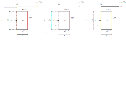
Figure 3: The cylinder $\mathsf{C}_{\alpha}$.

Constructions of two subdomains of $\Omega$: $\mathsf{C}_{\alpha}$ and $\Omega_{\mathsf{K}_{\alpha/2}}$. Define, for $\alpha>0$ small enough, the open cylinder

$$\mathsf{C}_{\alpha}=\big{\{}x\in\overline{\Omega},\,\mathsf{z}(x)\in\Gamma_{k,\mathbf{D}}^{\text{M}},\,x_{d}(x)\in(0,\alpha)\big{\}},$$ (135)

(see Figure 3 for a schematic representation of $\mathsf{C}_{\alpha}$), and the compact set

$$\mathsf{K}_{\alpha/2}=\big{\{}v\in\overline{\Omega},\ \mathsf{d}_{\,\overline{\Omega}}(v,\partial\Omega)\geq{\alpha}/{2}\big{\}}\subset\Omega.$$

From Proposition 29, there exists a $\mathcal{C}^{\infty}$ subdomain $\Omega_{\mathsf{K}_{\alpha/2}}$ of $\Omega$ containing $x_{0}$ such that $\mathsf{K}_{\alpha/2}\subset\Omega_{\mathsf{K}_{\alpha/2}}$, $\overline{\Omega_{\mathsf{K}_{\alpha/2}}}\subset\Omega$, and

$$\nabla f\cdot\mathsf{n}_{\Omega_{\mathsf{K}_{\alpha/2}}}>0\text{ on }\partial\Omega_{\mathsf{K}_{\alpha/2}}.$$ (136)

A schematic representation of $\Omega_{\mathsf{K}_{\alpha/2}}$ and $\mathsf{C}_{\alpha}$ is given in Figure 4.

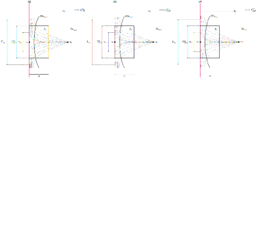
Figure 4: Schematic representations of $\mathsf{\Omega}_{k}^{\textsc{M}}=\mathsf{C}_{\alpha}\cup\Omega_{\mathsf{K}_{\alpha/2}}$, $\Gamma_{k,\mathbf{D}}^{\textsc{M}}$, and $\Gamma_{k,\mathbf{N}}^{\textsc{M}}$. On the right, a zoom in the neighborhood of $\Gamma_{z_{k}}$, where the dotted lines represent the flows of $\varphi_{x}$ near the saddle point $z_{k}$ of $f$ (see (12) and item 1 in ($\Omega$-$f$)).

Moreover it holds (see Figure 3):

$$\partial\mathsf{C}_{\alpha}=\overline{\Gamma_{k,\mathbf{D}}^{\text{M}}}\,\,\cup{\Sigma_{\alpha}^{lateral}}\,\cup\,\,\overline{\Sigma_{\alpha}^{base}},$$ (137)

where

$$\Sigma_{\alpha}^{lateral}=\big{\{}x\in\overline{\Omega},\,\mathsf{z}(x)\in\partial\Gamma_{k,\mathbf{D}}^{\text{M}},\,x_{d}(x)\in(0,\alpha)\big{\}}\subset\Omega,$$ (138)

and

$$\Sigma_{\alpha}^{base}=\big{\{}x\in\overline{\Omega},\,\mathsf{z}(x)\in\Gamma_{k,\mathbf{D}}^{\text{M}},\,x_{d}(x)=\alpha\big{\}}\subset\Omega.$$

Let us now prove that there exists $\alpha_{0}>0$, such that for all $\alpha\in(0,\alpha_{0})$, one has:

$$\nabla f\cdot\mathsf{n}_{\mathsf{C}_{\alpha}}>0\text{ on }\Sigma_{\alpha}^{lateral}.$$ (139)

It holds $\Sigma_{\alpha}^{lateral}=\big{\{}v\in\Omega,\,x_{1}(v)=0,\,x_{d}(v)\in(0,\alpha)\big{\}}$ (from  (131)–(133), (135),and  (138)), and hence, one has for all $v\in\Sigma_{\alpha}^{lateral}$:

$$\mathsf{n}_{\mathsf{C}_{\alpha}}(v)=-\frac{\nabla x_{1}(v)}{|\nabla x_{1}|(v)}.$$ (140)

Therefore, by a continuity argument, using (127) and (134), there exists $\alpha_{0}>0$ such that for all $\alpha\in(0,\alpha_{0})$ and for all $v\in\Sigma_{\alpha}^{lateral}$,

$$\nabla f(v)\cdot\mathsf{n}_{\mathsf{C}_{\alpha}}(v)>0.$$

This concludes the proof of (139).

Step 1b: definition of $\mathsf{\Omega}_{k}^{\textsc{M}}$ such that $\partial\mathsf{\Omega}_{k}^{\textsc{M}}\cap\partial\Omega=\overline{\Gamma_{k,\mathbf{D}}^{\text{M}}}$. Let us introduce (see Figure 4)

$$\mathsf{\Omega}_{k}^{\textsc{M}}:=\mathsf{C}_{\alpha}\cup\Omega_{\mathsf{K}_{\alpha/2}},$$ (141)

which is included in $\Omega$. Let us mention that $\mathsf{\Omega}_{k}^{\textsc{M}}$ depends on two parameters: $\alpha>0$ (through both $\mathsf{C}_{\alpha}$ and $\Omega_{\mathsf{K}_{\alpha/2}}$) and $\Gamma_{k,\mathbf{D}}^{\text{M}}$ (through $\mathsf{C}_{\alpha}$). One obviously has $\overline{\Gamma_{k,\mathbf{D}}^{\text{M}}}\subset\partial\mathsf{\Omega}_{k}^{\textsc{M}}$. Let us define

$$\Gamma_{k,\mathbf{N}}^{\text{M}}=\partial\mathsf{\Omega}_{k}^{\textsc{M}}\setminus\overline{\Gamma_{k,\mathbf{D}}^{\text{M}}},$$ (142)

so that $\partial\mathsf{\Omega}_{k}^{\textsc{M}}$ is the disjoint union of $\overline{\Gamma_{k,\mathbf{D}}^{\text{M}}}$ and $\Gamma_{k,\mathbf{N}}^{\text{M}}$. By definition, $\mathsf{\Omega}_{k}^{\textsc{M}}$ is the union of two intersecting open connected subsets $\mathsf{C}_{\alpha}$ and $\Omega_{\mathsf{K}_{\alpha/2}}$ of $\Omega$, it is thus open and connected. Notice that one has:

$$\partial\mathsf{\Omega}_{k}^{\textsc{M}}\subset\partial\mathsf{C}_{\alpha}\cup\partial\Omega_{\mathsf{K}_{\alpha/2}}$$ (143)

and, since $\overline{\Sigma_{\alpha}^{base}}\subset\mathsf{K}_{\alpha/2}\subset\Omega_{\mathsf{K}_{\alpha/2}}\subset\mathsf{\Omega}_{k}^{\textsc{M}}$ (see (137)), one has:

$$\partial\Omega_{\mathsf{K}_{\alpha/2}}\cap\overline{\Sigma_{\alpha}^{base}}=\emptyset\text{ and }\partial\mathsf{\Omega}_{k}^{\textsc{M}}\cap\overline{\Sigma_{\alpha}^{base}}=\emptyset.$$ (144)

In addition, from the fact that $\partial\Omega_{\mathsf{K}_{\alpha/2}}\subset\Omega$ and $\overline{\Gamma_{k,\mathbf{D}}^{\text{M}}}\subset\partial\Omega$, it holds:

$$\partial\Omega_{\mathsf{K}_{\alpha/2}}\cap\overline{\Gamma_{k,\mathbf{D}}^{\text{M}}}=\emptyset.$$ (145)

Thus, from (143), (144), and (145) together with the definition of $\Gamma_{k,\mathbf{N}}^{\text{M}}$, it holds: $\Gamma_{k,\mathbf{N}}^{\text{M}}\subset(\partial\mathsf{C}_{\alpha}\cup\partial\Omega_{\mathsf{K}_{\alpha/2}})\setminus(\overline{\Gamma_{k,\mathbf{D}}^{\text{M}}}\cup\overline{\Sigma_{\alpha}^{base}})=\partial\mathsf{C}_{\alpha}\setminus(\overline{\Gamma_{k,\mathbf{D}}^{\text{M}}}\cup\overline{\Sigma_{\alpha}^{base}})\cup\partial\Omega_{\mathsf{K}_{\alpha/2}}$ and thus, from (137),

$$\Gamma_{k,\mathbf{N}}^{\text{M}}\subset\Sigma_{\alpha}^{lateral}\cup\partial\Omega_{\mathsf{K}_{\alpha/2}}\subset\{v\in\Omega,\ \mathsf{d}_{\,\overline{\Omega}}(v,\partial\Omega)<{\alpha}\big{\}},$$ (146)

where the last inclusion follows from the fact that $\partial\Omega_{\mathsf{K}_{\alpha/2}}\subset\{v\in\Omega,\ \mathsf{d}_{\,\overline{\Omega}}(v,\partial\Omega)\leq\alpha/{2}\big{\}}$ and (138). In particular, this implies that, since $\overline{\Gamma_{k,\mathbf{D}}^{\text{M}}}\subset\partial\Omega$,

$$\partial\mathsf{\Omega}_{k}^{\textsc{M}}\cap\Omega=\Gamma_{k,\mathbf{N}}^{\text{M}}\text{ and }\partial\mathsf{\Omega}_{k}^{\textsc{M}}\cap\partial\Omega=\overline{\Gamma_{k,\mathbf{D}}^{\text{M}}}.$$ (147)

Step 2: Proofs of items 3 and 4 in Proposition 30.

Step 2a. Let us check that $\Gamma_{k,\mathbf{D}}^{\textsc{M}}$ and $\Gamma_{k,\mathbf{N}}^{\textsc{M}}$ meet at an angle strictly smaller than $\pi$ in $\mathsf{\Omega}_{k}^{\textsc{M}}$ (in the sense of Definition 31). To this end, let us prove that

$$\overline{\Gamma_{k,\mathbf{D}}^{\textsc{M}}}\cap\overline{\Gamma_{k,\mathbf{N}}^{\textsc{M}}}=\overline{\Gamma_{k,\mathbf{D}}^{\textsc{M}}}\cap\overline{\Sigma_{\alpha}^{lateral}}.$$ (148)

Notice that (148) implies that $\partial\mathsf{\Omega}_{k}^{\textsc{M}}$ is Lipschitz near $\overline{\Gamma_{k,\mathbf{D}}^{\textsc{M}}}\cap\overline{\Gamma_{k,\mathbf{N}}^{\textsc{M}}}$ as the union of the closures of two disjoint open transverse $\mathcal{C}^{\infty}$ hypersurfaces $\Gamma_{k,\mathbf{D}}^{\textsc{M}}$ and $\Sigma_{\alpha}^{lateral}$ (this will be used in Step 3b below). Furthermore, (148) implies that $\Gamma_{k,\mathbf{D}}^{\textsc{M}}$ and $\Gamma_{k,\mathbf{N}}^{\textsc{M}}$ meet at an angle $\pi/2$ (see Figure 5), which thus yields item 3 in Proposition 30.

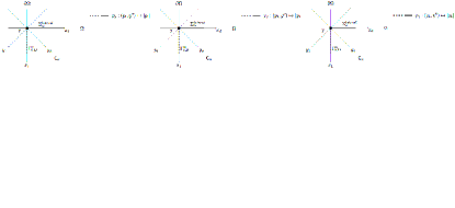
Figure 5: The sets $\Gamma_{k,\mathbf{D}}^{\textsc{M}}$ and $\Sigma_{\alpha}^{lateral}$ meet at an angle $\pi/2$ in $\mathsf{C}_{\alpha}$ (see Definition 31, (132), (133), and (137)). On the figure, $\mathsf{y}\in\overline{\Gamma_{k,\mathbf{D}}^{\textsc{M}}}\cap\overline{\Sigma_{\alpha}^{lateral}}$ and $\{x_{d}>0\}=\Omega$, $y_{1}=\frac{-x_{d}+x_{1}}{2}$, $y_{d}=\frac{x_{d}+x_{1}}{2}$, $y^{\prime\prime}=(x_{2},\dots,x_{d-1})$ (which is, schematically, the coordinates perpendicular to the plane $(x_{1},x_{d})$ centred at $\mathsf{y}$) , $\psi_{\mathsf{y}}(y^{\prime\prime})=0$, and $\varphi_{\mathsf{y}}(y_{1},y^{\prime\prime})=|y_{1}|$ in Definition 31.

Let us thus prove (148). From (146) together with (145), it holds: $\overline{\Gamma_{k,\mathbf{D}}^{\textsc{M}}}\cap\overline{\Gamma_{k,\mathbf{N}}^{\textsc{M}}}\subset\overline{\Gamma_{k,\mathbf{D}}^{\textsc{M}}}\cap\overline{\Sigma_{\alpha}^{lateral}}$. Now, let us consider $x\in\overline{\Gamma_{k,\mathbf{D}}^{\textsc{M}}}\cap\overline{\Sigma_{\alpha}^{lateral}}$. Then, there exists a sequence $(x_{n})_{n\geq 0}\in\Sigma_{\alpha}^{lateral}$ such that $x_{n}\to x$ as $n\to+\infty$. Let us prove that for all $n$ large enough, $x_{n}\in\partial\mathsf{\Omega}_{k}^{\textsc{M}}$. For $n$ large enough, $x_{n}$ does not belong to $\overline{\Omega_{\mathsf{K}_{\alpha/2}}}$ because $\overline{\Omega_{\mathsf{K}_{\alpha/2}}}\subset\Omega$ and $x_{n}\to x\in\partial\Omega$. In addition $x_{n}\notin\mathsf{C}_{\alpha}$ (indeed $x_{n}\in\partial\mathsf{C}_{\alpha}$ since $x_{n}\in\Sigma_{\alpha}^{lateral}$). Therefore, for $n$ large enough, $x_{n}\notin\mathsf{\Omega}_{k}^{\textsc{M}}.$ On the other hand, since $x_{n}\in\partial\mathsf{C}_{\alpha}$, $x_{n}\in\overline{\mathsf{C}_{\alpha}}\subset\overline{\mathsf{\Omega}_{k}^{\textsc{M}}}.$ In conclusion, $x_{n}\in\Omega\cap\partial{\mathsf{\Omega}_{k}^{\textsc{M}}}=\Gamma_{k,\mathbf{N}}^{\textsc{M}}$ (see (147)) and thus, $x\in\overline{\Gamma_{k,\mathbf{N}}^{\textsc{M}}}$. This concludes the proof of (148).

Step 2b. Let us now prove item 4 in Proposition 30. To this end, let $\delta>0$. Let us choose $\Gamma_{k,\mathbf{D}}^{\textsc{M}}$ such that the distance between $\overline{\Gamma_{k,\mathbf{D}}^{\textsc{M}}}$ and $\partial\Omega\setminus\Gamma_{z_{k}}$ is smaller than $\delta/2$ (recall that $\overline{\Gamma_{k,\mathbf{D}}^{\textsc{M}}}\subset\Gamma_{z_{k}}$ can be chosen as large as needed in $\Gamma_{z_{k}}$, see Step 1a above), i.e.

$$\mathsf{d}_{\,\overline{\Omega}}(\overline{\Gamma_{k,\mathbf{D}}^{\textsc{M}}},\partial\Omega\setminus\Gamma_{z_{k}})\leq\delta/2.$$ (149)

Let us consider $x\in\Gamma_{k,\mathbf{N}}^{\textsc{M}}$. According to (146), $x\in\Sigma_{\alpha}^{lateral}$ or $x\in\partial\Omega_{\mathsf{K}_{\alpha/2}}$. If $x\in\Sigma_{\alpha}^{lateral}$, then by the triangular inequality, it holds:

$$\mathsf{d}_{\,\overline{\Omega}}(x,\partial\Omega\setminus\Gamma_{z_{k}})\leq\mathsf{d}_{\,\overline{\Omega}}(x,\overline{\Gamma_{k,\mathbf{D}}^{\textsc{M}}})+\mathsf{d}_{\,\overline{\Omega}}(\overline{\Gamma_{k,\mathbf{D}}^{\textsc{M}}},\partial\Omega\setminus\Gamma_{z_{k}})\leq\alpha+\delta/2,$$

where we have used that according to (138), $\mathsf{d}_{\,\overline{\Omega}}(x,\overline{\Gamma_{k,\mathbf{D}}^{\textsc{M}}})\leq\mathsf{d}_{\,\overline{\Omega}}(x,\partial{\Gamma_{k,\mathbf{D}}^{\textsc{M}}})\leq\alpha$, for all $x\in\Sigma_{\alpha}^{lateral}$. If $x\in\partial\Omega_{\mathsf{K}_{\alpha/2}}$, then $\mathsf{d}_{\,\overline{\Omega}}(x,\partial\Omega)\leq\alpha/2<\alpha$. Because $x\notin\mathsf{C}_{\alpha}$ (since $x\in\partial\mathsf{\Omega}_{k}^{\textsc{M}}$ and $\mathsf{C}_{\alpha}$ is an open subset of $\mathsf{\Omega}_{k}^{\textsc{M}}$), one has $\mathsf{z}(x)\in\partial\Omega\setminus\Gamma_{k,\mathbf{D}}^{\textsc{M}}$. Therefore,

$$\mathsf{d}_{\,\overline{\Omega}}(x,\partial\Omega\setminus\Gamma_{z_{k}})\leq\mathsf{d}_{\,\overline{\Omega}}(x,\mathsf{z}(x))+\mathsf{d}_{\,\overline{\Omega}}(\mathsf{z}(x),\partial\Omega\setminus\Gamma_{z_{k}})\leq\alpha/2+\delta/2,$$

where we have used that either $\mathsf{z}(x)\in\partial\Omega\setminus\Gamma_{z_{k}}$ (in which case $\mathsf{d}_{\,\overline{\Omega}}(\mathsf{z}(x),\partial\Omega\setminus\Gamma_{z_{k}})=0$) or $\mathsf{z}(x)\in\Gamma_{z_{k}}\setminus\Gamma_{k,\mathbf{D}}^{\textsc{M}}$ (in which case $\mathsf{d}_{\,\overline{\Omega}}(\mathsf{z}(x),\partial\Omega\setminus\Gamma_{z_{k}})\leq\delta/2$, see (149) together with the fact that $\mathsf{z}(x)\notin\Gamma_{k,\mathbf{D}}^{\textsc{M}}$). In conclusion

$$\sup_{x\in\Gamma_{k,\mathbf{N}}^{\textsc{M}}}\mathsf{d}_{\,\overline{\Omega}}(x,\partial\Omega\setminus\Gamma_{z_{k}})\leq\alpha+\delta/2.$$

Choosing $\alpha\leq\delta/2$ concludes the proof of item 4 in Proposition 30.

Step 3: Proof that $\mathsf{\Omega}_{k}^{\textsc{M}}$ is Lipschitz, and study of the sign of $\nabla f\cdot\mathsf{n}_{\mathsf{\Omega}_{k}^{\textsc{M}}}$. Let us first check that $\mathsf{\Omega}_{k}^{\textsc{M}}$ is Lipschitz. Notice that the union of two Lipchitz (even smooth) subdomains of $\Omega$ is not necessarily a Lipchitz domain (the boundary is even not necessarily a manifold). In our setting, one has:

$$\partial\Omega_{\mathsf{K}_{\alpha/2}}\cap\partial\mathsf{C}_{\alpha}=\partial\Omega_{\mathsf{K}_{\alpha/2}}\cap\Sigma_{\alpha}^{lateral}\text{ (see~{}\eqref{eq.3P},~{}\eqref{eq.unionboundary2}, and~{}\eqref{eq.unionboundary3})},$$

where (i) $\Sigma_{\alpha}^{lateral}$ and $\partial\Omega_{\mathsf{K}_{\alpha/2}}$ are smooth, and (ii) the normal derivatives $\nabla f(v)\cdot\mathsf{n}_{\mathsf{C}_{\alpha}}(v)$ and $\nabla f(v)\cdot\mathsf{n}_{\Omega_{\mathsf{K}_{\alpha/2}}}(v)$ of $f$ at $v\in\Sigma_{\alpha}^{lateral}\cap\partial\Omega_{\mathsf{K}_{\alpha/2}}$ are positive (so that the two normal vectors cannot be opposite, a situation which could create cusps). These two points will be used to prove that the boundary of $\mathsf{\Omega}_{k}^{\textsc{M}}$ is Lipschitz. One has:

$$\partial\mathsf{\Omega}_{k}^{\textsc{M}}\subset\partial\Omega_{\mathsf{K}_{\alpha/2}}\cup\partial\mathsf{C}_{\alpha}.$$ (150)

Define the two open subsets of $\partial\mathsf{\Omega}_{k}^{\textsc{M}}$

$$\mathsf{A}_{1}:=\partial\mathsf{\Omega}_{k}^{\textsc{M}}\cap(\partial\Omega_{\mathsf{K}_{\alpha/2}}\setminus\partial\mathsf{C}_{\alpha}),\ \ \,\mathsf{A}_{2}:=\partial\mathsf{\Omega}_{k}^{\textsc{M}}\cap(\partial\mathsf{C}_{\alpha}\setminus\partial\Omega_{\mathsf{K}_{\alpha/2}}),$$ (151)

and the closed subset of $\partial\mathsf{\Omega}_{k}^{\textsc{M}}$ $\mathsf{A}_{3}:=\partial\mathsf{\Omega}_{k}^{\textsc{M}}\cap(\partial\Omega_{\mathsf{K}_{\alpha/2}}\cap\partial\mathsf{C}_{\alpha}),$ so that $\partial\mathsf{\Omega}_{k}^{\textsc{M}}$ is the disjoint union of $\mathsf{A}_{1}$, $\mathsf{A}_{2}$, and $\mathsf{A}_{3}$. Let us now prove that, for $j\in\{1,2,3\}$, $\partial\mathsf{\Omega}_{k}^{\textsc{M}}$ is Lipschitz in a neighborhood of any point of $\mathsf{A}_{j}$, and let us also study the sign of $\nabla f\cdot\mathsf{n}_{\mathsf{\Omega}_{k}^{\textsc{M}}}$ on $\mathsf{A}_{j}$.

Step 3a: Study of $\mathsf{A}_{1}$. First notice that (because $\partial\Omega_{\mathsf{K}_{\alpha/2}}\subset\Omega$),

$$\mathsf{A}_{1}\subset\partial\Omega_{\mathsf{K}_{\alpha/2}}\setminus\partial\mathsf{C}_{\alpha}\subset\Omega,$$ (152)

Let $z\in\mathsf{A}_{1}$. Then, there exists a neighborhood $\mathsf{O}_{z}$ of $z$ in $\mathbb{R}^{d}$ such that $\mathsf{O}_{z}\cap\overline{\mathsf{C}_{\alpha}}=\emptyset$. Indeed, if not, $z$ would belong to $\overline{\mathsf{C}_{\alpha}}=\partial\mathsf{C}_{\alpha}\cup\mathsf{C}_{\alpha}$, and $z$ cannot belong to $\partial\mathsf{C}_{\alpha}$ (by definition of $\mathsf{A}_{1}$) and $z$ cannot belong to $\mathsf{C}_{\alpha}$ (because $z\in\partial\mathsf{\Omega}_{k}^{\textsc{M}}$). Using (141), it then holds $\mathsf{O}_{z}\cap\overline{\mathsf{\Omega}_{k}^{\textsc{M}}}=\mathsf{O}_{z}\cap\overline{\Omega_{\mathsf{K}_{\alpha/2}}}$ (because $\overline{\mathsf{\Omega}_{k}^{\textsc{M}}}=\overline{\mathsf{C}_{\alpha}}\cup\overline{\Omega_{\mathsf{K}_{\alpha/2}}}$). Therefore, since in addition $\Omega_{\mathsf{K}_{\alpha/2}}$ is a smooth domain, $\mathsf{A}_{1}$ is a smooth part of the boundary of $\mathsf{\Omega}_{k}^{\textsc{M}}$ and $\mathsf{n}_{\mathsf{\Omega}_{k}^{\textsc{M}}}=\mathsf{n}_{\Omega_{\mathsf{K}_{\alpha/2}}}$ on $\mathsf{A}_{1}$. Finally, using (136), it holds:

$$\partial_{\mathsf{n}_{\mathsf{\Omega}_{k}^{\textsc{M}}}}f>0\text{ on }\mathsf{A}_{1}.$$ (153)

Step 3b: Study of $\mathsf{A}_{2}$. It holds $\mathsf{A}_{2}\subset\partial\mathsf{C}_{\alpha}\setminus\partial\Omega_{\mathsf{K}_{\alpha/2}}$. With the same arguments as in Step 3a (see the lines after (152)), $\mathsf{O}_{z}\cap\overline{\mathsf{\Omega}_{k}^{\textsc{M}}}=\mathsf{O}_{z}\cap\overline{\mathsf{C}_{\alpha}}$ for some neighborhood $\mathsf{O}_{z}$ af any point $z\in\mathsf{A}_{2}$. Moreover, from (137), $\partial\mathsf{C}_{\alpha}$ is $\mathcal{C}^{\infty}$ except on $\partial{\Gamma_{k,\mathbf{D}}^{\textsc{M}}}\cup\partial\Sigma_{\alpha}^{base}$, where it is Lipschitz since $\Gamma_{k,\mathbf{D}}^{\textsc{M}}$ and $\Sigma_{\alpha}^{lateral}$, and $\Sigma_{\alpha}^{base}$ and $\Sigma_{\alpha}^{lateral}$ are transverse (see Step 2a above). Thus, $\mathsf{A}_{2}$ is a Lipschitz part of the boundary of $\mathsf{\Omega}_{k}^{\textsc{M}}$ and

$$\mathsf{n}_{\mathsf{\Omega}_{k}^{\textsc{M}}}=\mathsf{n}_{\mathsf{C}_{\alpha}}\ \text{ on $\mathsf{A}_{2}\setminus(\partial{\Gamma_{k,\mathbf{D}}^{\textsc{M}}}\cup\partial\Sigma_{\alpha}^{base})$, i.e. a.e. on $\mathsf{A}_{2}$}.$$ (154)

Let us now study the sign of $\nabla f\cdot\mathsf{n}_{\mathsf{\Omega}_{k}^{\textsc{M}}}$ on $\mathsf{A}_{2}$. Recall that $\partial\mathsf{C}_{\alpha}=\overline{\Gamma_{k,\mathbf{D}}^{\textsc{M}}}\cup{\Sigma_{\alpha}^{lateral}}\cup\overline{\Sigma_{\alpha}^{base}}$ (see (137)), $\overline{\Gamma_{k,\mathbf{D}}^{\textsc{M}}}\cap\partial\Omega_{\mathsf{K}_{\alpha/2}}=\emptyset$ (see indeed (145)), and $\partial\mathsf{\Omega}_{k}^{\textsc{M}}\cap\overline{\Sigma_{\alpha}^{base}}=\emptyset$ (see (144)). Hence, it holds:

$$\mathsf{A}_{2}=\partial\mathsf{\Omega}_{k}^{\textsc{M}}\cap(\partial\mathsf{C}_{\alpha}\setminus\partial\Omega_{\mathsf{K}_{\alpha/2}}) =\underbrace{(\partial\mathsf{\Omega}_{k}^{\textsc{M}}\cap\overline{\Gamma_{k,\mathbf{D}}^{\textsc{M}}})}_{=\overline{\Gamma_{k,\mathbf{D}}^{\textsc{M}}}}\cup(\partial\mathsf{\Omega}_{k}^{\textsc{M}}\cap{\Sigma_{\alpha}^{lateral}}\setminus\partial\Omega_{\mathsf{K}_{\alpha/2}}).$$ (155)

Let $z\in\mathsf{A}_{2}$. If $z\in\Gamma_{k,\mathbf{D}}^{\textsc{M}}$, then $\mathsf{n}_{\mathsf{C}_{\alpha}}(z)=\mathsf{n}_{\Omega}(z)$ and thus, using (154), it holds:

$$\nabla f\cdot\mathsf{n}_{\mathsf{\Omega}_{k}^{\textsc{M}}}=0\text{ on }{\Gamma_{k,\mathbf{D}}^{\textsc{M}}},$$ (156)

where we also used the fact that $\Gamma_{k,\mathbf{D}}^{\textsc{M}}\subset\Gamma_{z_{k}}$ together with item 2 in ($\Omega$-$f$). If $z\in\Sigma_{\alpha}^{lateral}$, then from (139) and (154), it holds,

$$\nabla f\cdot\mathsf{n}_{\mathsf{\Omega}_{k}^{\textsc{M}}}>0\text{ on }\partial\mathsf{\Omega}_{k}^{\textsc{M}}\cap{\Sigma_{\alpha}^{lateral}}\setminus\partial\Omega_{\mathsf{K}_{\alpha/2}}.$$ (157)

Step 3c: Study of $\mathsf{A}_{3}$. Notice that $\mathsf{A}_{3}=\partial\Omega_{\mathsf{K}_{\alpha/2}}\cap\partial\mathsf{C}_{\alpha}$ (because $\partial\Omega_{\mathsf{K}_{\alpha/2}}\cap\partial\mathsf{C}_{\alpha}\subset\partial\mathsf{\Omega}_{k}^{\textsc{M}}$). Notice also that since $\partial\Omega_{\mathsf{K}_{\alpha/2}}\subset\Omega$,

$$\mathsf{A}_{3}\subset\Omega$$ (158)

Using (137), (144), and (145), it holds:

$$\mathsf{A}_{3}=\partial\Omega_{\mathsf{K}_{\alpha/2}}\cap\partial\mathsf{C}_{\alpha}=\partial\Omega_{\mathsf{K}_{\alpha/2}}\cap\Sigma_{\alpha}^{lateral}.$$ (159)

Thus, $\partial\Omega_{\mathsf{K}_{\alpha/2}}$ intersects $\partial\mathsf{C}_{\alpha}$ where $\partial\mathsf{C}_{\alpha}$ is smooth (i.e. on $\Sigma_{\alpha}^{lateral}$). Let us consider $v\in\mathsf{A}_{3}$. Let us conclude the proof by considering successively the case when $\mathsf{n}_{\Omega_{\mathsf{K}_{\alpha/2}}}(v)$ is not collinear to $\mathsf{n}_{\mathsf{C}_{\alpha}}(v)$, and the case when $\mathsf{n}_{\Omega_{\mathsf{K}_{\alpha/2}}}(v)=\pm\mathsf{n}_{\mathsf{C}_{\alpha}}(v)$.

Let us first consider the case when $\mathsf{n}_{\Omega_{\mathsf{K}_{\alpha/2}}}(v)$ is not collinear to $\mathsf{n}_{\mathsf{C}_{\alpha}}(v)$. By a continuity argument, there exists a neighborhood $\mathsf{O}_{v}$ of $v$ in $\Omega$ such that $\mathsf{O}_{v}\cap\partial\mathsf{C}_{\alpha}=\mathsf{O}_{v}\cap\Sigma_{\alpha}^{lateral}$ (so that $\mathsf{n}_{\mathsf{C}_{\alpha}}$ is defined everywhere and continuous on $\mathsf{O}_{v}\cap\partial\mathsf{C}_{\alpha}$) and such that $\mathsf{n}_{\Omega_{\mathsf{K}_{\alpha/2}}}$ is not collinear to $\mathsf{n}_{\mathsf{C}_{\alpha}}$ on $\mathsf{O}_{v}$. Consequently, $\partial\Omega_{\mathsf{K}_{\alpha/2}}$ and $\partial\mathsf{C}_{\alpha}$ are transverse on $\mathsf{O}_{v}$ (or equivalently, the natural immersion map $\mathsf{i}:\partial\Omega_{\mathsf{K}_{\alpha/2}}\to\mathbb{R}^{d}$ is transverse to $\partial\mathsf{C}_{\alpha}$ on $\mathsf{O}_{v}$). Thus, $\mathsf{O}_{v}\cap\partial\mathsf{\Omega}_{k}^{\textsc{M}}$ is Lipschitz. In addition, as a consequence of the inverse image of a regular value Theorem [11, Theorem (5.12)] and its proof (see also [85, 70, 36]) applied here to the smooth function $\mathsf{i}$, one has, up to choosing $\mathsf{O}_{v}$ smaller, $\mathsf{O}_{v}\cap\mathsf{i}^{-1}(\partial\mathsf{C}_{\alpha})=\mathsf{O}_{v}\cap(\partial\Omega_{\mathsf{K}_{\alpha/2}}\cap\partial\mathsf{C}_{\alpha})$ (because $\mathsf{i}^{-1}(\partial\mathsf{C}_{\alpha})=\partial\Omega_{\mathsf{K}_{\alpha/2}}\cap\partial\mathsf{C}_{\alpha}$) is a $1$-codimensional smooth submanifold of $\partial\Omega_{\mathsf{K}_{\alpha/2}}$ (i.e. a $2$-codimensional smooth submanifold of $\mathbb{R}^{d}$ included in $\partial\mathsf{\Omega}_{k}^{\textsc{M}}$). Therefore, for all $v\in\mathsf{A}_{3}$ such that $\mathsf{n}_{\Omega_{\mathsf{K}_{\alpha/2}}}(v)$ is not collinear to $\mathsf{n}_{\mathsf{C}_{\alpha}}(v)$, there exists a neighborhood $\mathsf{O}_{v}$ of $v$ in $\Omega$ such that

$$\text{$\mathsf{O}_{v}\cap\mathsf{A}_{3}$ is of measure $0$ for the surface measure on $\mathsf{O}_{v}\cap\partial\mathsf{\Omega}_{k}^{\textsc{M}}$}.$$ (160)

Let us finally consider the case when $\mathsf{n}_{\Omega_{\mathsf{K}_{\alpha/2}}}(v)=\pm\mathsf{n}_{\mathsf{C}_{\alpha}}(v)$. Using (136) and (139), $\mathsf{n}_{\Omega_{\mathsf{K}_{\alpha/2}}}(v)=+\mathsf{n}_{\mathsf{C}_{\alpha}}(v)$. Moreover, from (135), (138), and (159) there exists a neighborhood $\mathsf{O}_{v}$ of $v$ in $\Omega$ such that $\mathsf{O}_{v}\cap\partial\mathsf{C}_{\alpha}=\mathsf{O}_{v}\cap\Sigma_{\alpha}^{lateral}$ and thus (see (132) and (133)),

$$\mathsf{O}_{v}\cap\mathsf{C}_{\alpha}=\mathsf{O}_{v}\cap\big{\{}w\in\overline{\Omega},\,x_{1}(w)>0,\,x_{d}(w)\in(0,\alpha)\big{\}}$$

and (see (138))

$$\mathsf{O}_{v}\cap\partial\mathsf{C}_{\alpha}=\mathsf{O}_{v}\cap\big{\{}w\in\overline{\Omega},\,x_{1}(w)=0,\,x_{d}(w)\in(0,\alpha)\big{\}}\ (=\mathsf{O}_{v}\cap\Sigma_{\alpha}^{lateral}).$$ (161)

In the following, with a slight abuse of notation, we will denote by $x=(x_{1},\tilde{x})$ both a point in $\mathsf{O}_{v}$ and its coordinates in the local basis.

In addition, since $\mathsf{n}_{\Omega_{\mathsf{K}_{\alpha/2}}}(v)=+\mathsf{n}_{\mathsf{C}_{\alpha}}(v)$ and $\partial\Omega_{\mathsf{K}_{\alpha}}$ is smooth, up to choosing $\mathsf{O}_{v}$ smaller, there exists a smooth function $\Psi:\mathbb{R}^{d-1}\to\mathbb{R}$ such that $\Psi(\tilde{x}(v))=x_{1}(v)=0$ and

$$\mathsf{O}_{v}\cap\partial\Omega_{\mathsf{K}_{\alpha/2}}=\{(\Psi(\tilde{x}),\tilde{x}),\,x=(x_{1},\tilde{x})\in\mathsf{O}_{v}\}$$ (162)

is the graph of $\Psi$ in the $(x_{1},\tilde{x})$ coordinates, where we set $\tilde{x}:=(x_{2},\ldots,x_{d-1},x_{d})$. Moreover, one has

$$\mathsf{O}_{v}\cap\Omega_{\mathsf{K}_{\alpha/2}}=\{x=(x_{1},\tilde{x})\in\mathsf{O}_{v}\text{ such that }\,x_{1}>\Psi(\tilde{x})\}.$$

Therefore, from (141), $\mathsf{O}_{v}\cap\mathsf{\Omega}_{k}^{\textsc{M}}=\{x=(x_{1},\tilde{x})\in\mathsf{O}_{v}\text{ such that }\,x_{1}>\min(\Psi(\tilde{x}),0)\}$ and thus,

$$\mathsf{O}_{v}\cap\partial\mathsf{\Omega}_{k}^{\textsc{M}}=\{x=(x_{1},\tilde{x})\in\mathsf{O}_{v}\text{ such that }\,x_{1}=\min(\Psi(\tilde{x}),0)\}$$

is Lipschitz (indeed $\Upsilon:\tilde{x}\mapsto\min(\Psi(\tilde{x}),0)$ is a Lipschitz function). In addition, for a.e. $x=(x_{1},\tilde{x})\in\mathsf{O}_{v}\cap\partial\mathsf{\Omega}_{k}^{\textsc{M}}$: $\mathsf{n}_{\mathsf{\Omega}_{k}^{\textsc{M}}}(x)\in\{\mathsf{n}_{\mathsf{C}_{\alpha}}(x),\mathsf{n}_{\Omega_{\mathsf{K}_{\alpha}}}(x)\}$. Indeed, in the $(x_{1},\tilde{x})$-coordinates, one has for a.e. $x=(x_{1},\tilde{x})\in\mathsf{O}_{v}\cap\partial\mathsf{\Omega}_{k}^{\textsc{M}}$,

$$T_{x}\partial\mathsf{\Omega}_{k}^{\textsc{M}}=\Big{\{}\big{(}\tilde{p}\cdot\nabla\Upsilon(\tilde{x}),\tilde{p}\big{)},\ \tilde{p}\in\mathbb{R}^{d-1}\Big{\}}\text{ and }\mathsf{n}_{\mathsf{\Omega}_{k}^{\textsc{M}}}(x)=\frac{(-1,\nabla\Upsilon(\tilde{x}))}{\sqrt{1+|\nabla\Upsilon(\tilde{x})|^{2}}}.$$

Because for a.e. $\tilde{x}$, $\nabla\Upsilon(\tilde{x})\in\{0,\nabla\Psi(\tilde{x})\}$, it holds for a.e. $x=(x_{1},\tilde{x})\in\mathsf{O}_{v}\cap\partial\mathsf{\Omega}_{k}^{\textsc{M}}$, $\mathsf{n}_{\mathsf{\Omega}_{k}^{\textsc{M}}}(x)\in\{\mathsf{n}_{\mathsf{C}_{\alpha}}(x),\mathsf{n}_{\Omega_{\mathsf{K}_{\alpha}}}(x)\}$. Moreover, using (136) and (139), it holds for a.e. $x=(x_{1},\tilde{x})\in\mathsf{O}_{v}\cap\partial\mathsf{\Omega}_{k}^{\textsc{M}}$:

$$\nabla f(x)\cdot\mathsf{n}_{\mathsf{\Omega}_{k}^{\textsc{M}}}(x)>0.$$ (163)

From (160) and (163), we thus conclude that for any point $v\in\mathsf{A}_{3}$, there exists a neighborhood $\mathsf{O}_{v}$ of $v$ in $\Omega$ such that, for the surface measure on $\mathsf{O}_{v}\cap\partial\mathsf{\Omega}_{k}^{\textsc{M}}$, either $\mathsf{O}_{v}\cap\mathsf{A}_{3}$ is of measure $0$ or $\nabla f\cdot\mathsf{n}_{\mathsf{\Omega}_{k}^{\textsc{M}}}>0$ a.e. on $\mathsf{O}_{v}\cap\mathsf{A}_{3}$. This implies that, for the surface measure on $\partial\mathsf{\Omega}_{k}^{\textsc{M}}$,

$$\nabla f\cdot\mathsf{n}_{\mathsf{\Omega}_{k}^{\textsc{M}}}>0\text{ a.e. on }\mathsf{A}_{3}.$$ (164)

In conclusion, $\mathsf{\Omega}_{k}^{\textsc{M}}$ is a Lipschitz subdomain of $\Omega$. Furthermore, we have proved that:

$$\nabla f\cdot\mathsf{n}_{\mathsf{\Omega}_{k}^{\textsc{M}}}=0\text{ a.e. on }\overline{\Gamma_{k,\mathbf{D}}^{\textsc{M}}}=\partial\mathsf{\Omega}_{k}^{\textsc{M}}\cap\partial\Omega\ \text{ (see~{}\eqref{eq.panf2} and~{}\eqref{eq.onm})}.$$

In addition, since (see (147), (152), (155), and (158))

$$\Gamma_{k,\mathbf{N}}^{\textsc{M}}=\partial\mathsf{\Omega}_{k}^{\textsc{M}}\cap\Omega=\mathsf{A}_{1}\,\cup\,(\mathsf{A}_{2}\ \cap\ \Omega)\,\cup\,\mathsf{A}_{3},$$

and $\mathsf{A}_{2}\ \cap\ \Omega=\partial\mathsf{\Omega}_{k}^{\textsc{M}}\cap{\Sigma_{\alpha}^{lateral}}\setminus\partial\Omega_{\mathsf{K}_{\alpha/2}}$, one deduces from (153), (157), and (164), that

$$\nabla f\cdot\mathsf{n}_{\mathsf{\Omega}_{k}^{\textsc{M}}}>0\text{ a.e. on }\Gamma_{k,\mathbf{N}}^{\textsc{M}}=\partial\mathsf{\Omega}_{k}^{\textsc{M}}\cap\Omega.$$

This concludes the proof of Proposition 30.    

Witten Laplacians with mixed Dirichlet-Neumann boundary conditions associated with $(z_{k})_{k=1,\ldots,n}$

In this section, we define a Witten Laplacian with mixed Dirichlet-Neumann boundary conditions associated with each saddle point $z_{k}$ of $f$ using the domain $\mathsf{\Omega}_{k}^{\textsc{M}}$ constructed in the previous section. The idea is to define a Witten Laplacian in $\Lambda^{q}L^{2}(\mathsf{\Omega}_{k}^{\textsc{M}})$ with Dirichlet boundary conditions on $\Gamma_{k,\mathbf{D}}^{\textsc{M}}$ (where $\nabla f\cdot\mathsf{n}_{\mathsf{\Omega}_{k}^{\textsc{M}}}=0$) and Neumann boundary conditions on $\Gamma_{k,\mathbf{N}}^{\textsc{M}}$ (where $\nabla f\cdot\mathsf{n}_{\mathsf{\Omega}_{k}^{\textsc{M}}}>0$), see Proposition 30. Since $x_{0}\in\mathsf{\Omega}_{k}^{\textsc{M}}$ is the only minimum of $f$ in $\mathsf{\Omega}_{k}^{\textsc{M}}$ and $z_{k}\in\partial\mathsf{\Omega}_{k}^{\textsc{M}}$ is the only saddle point of $f$ in $\overline{\mathsf{\Omega}_{k}^{\textsc{M}}}$, we expect, in view of Theorem 4 and the results of [56], that such Witten Laplacians have only one eigenvalue smaller than $\mathsf{c}h$ when $q=0$ and $q=1$. Thanks to Witten’s complex structure, this eigenvalue, already introduced as $\lambda(\mathsf{\Omega}_{k}^{\textsc{M}})$ at the beginning of Section 3, will be the same for $q=0$ and $q=1$. The quasi-mode $\mathsf{v}_{k}^{(1)}$ of $\Delta_{f,h}^{\mathsf{Di},(1)}(\Omega)$ associated with $z_{k}$ will then be defined by multiplying by a cut-off function the principal $1$-eigenform $\mathsf{u}_{k}^{(1)}$ of this Witten Laplacian with mixed Dirichlet-Neumann boundary conditions.

We first give the definition of Witten Laplacians with mixed Dirichlet-Neumann boundary conditions on Lipschitz domains in Section 3.3.1. We then study the spectral properties of these Witten Laplacians and derive some estimates on the principal eigenvalues and eigenforms in Sections 3.3.2, 3.3.3 and 3.3.4

Witten Laplacians with mixed Dirichlet-Neumann boundary conditions on Lipschitz domains

In this section, in order to ease the notation, we drop the subscript $k$ in $(\mathsf{\Omega}^{\textsc{M}}_{k},\Gamma^{\textsc{M}}_{k,\mathbf{D}},\Gamma^{\textsc{M}}_{k,\mathbf{N}})$, since the results will then be applied to each of this triplet, for $k\in\{1,\ldots,n\}$. Let thus $\mathsf{\Omega}^{\textsc{M}}$ be a Lipschitz subdomain of $\Omega$. Let $\Gamma^{\textsc{M}}_{\mathbf{D}}$ and $\Gamma^{\textsc{M}}_{\mathbf{N}}$ be two disjoint open subsets of $\partial\mathsf{\Omega}^{\textsc{M}}$ such that $\overline{\Gamma^{\textsc{M}}_{\mathbf{D}}}\cup\overline{\Gamma^{\textsc{M}}_{\mathbf{N}}}=\partial\mathsf{\Omega}^{\textsc{M}}$.

This section is organized as follows. We first recall the definition of weak traces for forms $w\in\Lambda^{q}H_{\mathsf{d}}(\mathsf{\Omega}^{\textsc{M}})\cap\Lambda^{q}H_{\mathsf{d}^{*}}(\mathsf{\Omega}^{\textsc{M}})$ where for $q\in\{0,\ldots,d\}$,

$$\Lambda^{q}H_{\mathsf{d}}(\mathsf{\Omega}^{\textsc{M}}):=\left\{w\in\Lambda^{q}L^{2}(\mathsf{\Omega}^{\textsc{M}}),\ \mathsf{d}w\in\Lambda^{q+1}L^{2}(\mathsf{\Omega}^{\textsc{M}})\right\}$$ (165)

and

$$\Lambda^{q}H_{\mathsf{d}^{*}}(\mathsf{\Omega}^{\textsc{M}})\ :=\ \left\{w\in\Lambda^{q}L^{2}(\mathsf{\Omega}^{\textsc{M}}),\ \mathsf{d}^{*}w\in\Lambda^{q-1}L^{2}(\mathsf{\Omega}^{\textsc{M}})\right\}$$ (166)

are equipped with their natural graph norms. Let us recall the convention $\Lambda^{-1}L^{2}=\Lambda^{d+1}L^{2}=\{0\}$. Secondly, we state trace estimates and subelliptic estimates for forms $w\in\Lambda^{q}H_{\mathsf{d}}(\mathsf{\Omega}^{\textsc{M}})\cap\Lambda^{q}H_{\mathsf{d}^{*}}(\mathsf{\Omega}^{\textsc{M}})$ such that $\mathbf{t}w=0$ on $\Gamma^{\textsc{M}}_{\mathbf{D}}$ and $\mathbf{n}w=0$ on $\Gamma^{\textsc{M}}_{\mathbf{N}}$. Indeed (see [12, 49]), a trace in $\Lambda^{q}L^{2}(\partial\mathsf{\Omega}^{\textsc{M}})$ does not exist in general for such forms except if $\Gamma^{\textsc{M}}_{\mathbf{D}}$ and $\Gamma^{\textsc{M}}_{\mathbf{N}}$ meet at an angle strictly smaller than $\pi$ (measured in $\mathsf{\Omega}^{\textsc{M}}$), in the sense of Definition 31. This explains the role of item $3$ in Proposition 30. Finally, we introduce the Witten Laplacians of interest, together with an associated Green formula. This formula will be crucial to study the spectral properties of these operators in the next section.

Weak definitions of traces for elements in $\Lambda^{q}H_{\mathsf{d}}(\mathsf{\Omega}^{\textsc{M}})$ or in $\Lambda^{q}H_{\mathsf{d}^{*}}(\mathsf{\Omega}^{\textsc{M}})$. Let us recall that for a differential form $u$ in $\Lambda^{q}L^{2}(\partial\mathsf{\Omega}^{\textsc{M}})$, the tangential and normal components are defined as follows:

$$u=\mathbf{t}u+\mathbf{n}u\quad\text{with}\quad\mathbf{t}u=\mathbf{i}_{\mathsf{n}_{\mathsf{\Omega}^{\textsc{M}}}}(\mathsf{n}_{\mathsf{\Omega}^{\textsc{M}}}^{\flat}\wedge u)\quad\text{and}\quad\mathbf{n}u=\mathsf{n}_{\mathsf{\Omega}^{\textsc{M}}}^{\flat}\wedge(\mathbf{i}_{\mathsf{n}_{\mathsf{\Omega}^{\textsc{M}}}}u),$$ (167)

where the superscript $\flat$ stands for the usual musical isomorphism ($\mathsf{n}_{\mathsf{\Omega}^{\textsc{M}}}^{\flat}$ is the 1-form associated with $\mathsf{n}_{\mathsf{\Omega}^{\textsc{M}}}$, $\mathsf{n}_{\mathsf{\Omega}^{\textsc{M}}}$ being is the unit outward normal to $\mathsf{\Omega}^{\textsc{M}}$). Notice that $\mathbf{t}u$ is orthogonal to $\mathbf{n}u$ in $\Lambda^{q}L^{2}(\partial\mathsf{\Omega}^{\textsc{M}})$. Let us recall that the mapping

$$w\in\Lambda^{q}H^{1}(\mathsf{\Omega}^{\textsc{M}})\mapsto w|_{\partial\mathsf{\Omega}^{\textsc{M}}}\in\Lambda^{q}H^{1/2}(\partial\mathsf{\Omega}^{\textsc{M}})$$ (168)

is well defined, continuous, and surjective. We would like here to recall the procedure to extend the notion of traces to elements in the subspaces of $\Lambda^{q}H^{1}(\mathsf{\Omega}^{\textsc{M}})$: $\Lambda^{q}H_{\mathsf{d}}(\mathsf{\Omega}^{\textsc{M}})$ and $\Lambda^{q}H_{\mathsf{d}^{*}}(\mathsf{\Omega}^{\textsc{M}})$. This is achieved using a duality argument and the standard Green formula which reads for differential forms $(u,v)\in\Lambda^{q}H^{1}(\mathsf{\Omega}^{\textsc{M}})\times\Lambda^{q+1}H^{1}(\mathsf{\Omega}^{\textsc{M}})$:

$$\langle\mathsf{d}u,v\rangle_{L^{2}(\mathsf{\Omega}^{\textsc{M}})}-\langle u,\mathsf{d}^{*}v\rangle_{L^{2}(\mathsf{\Omega}^{\textsc{M}})} =\int_{\partial\mathsf{\Omega}^{\textsc{M}}}\langle\mathsf{n}_{\mathsf{\Omega}^{\textsc{M}}}^{\flat}\wedge u,v\rangle_{T^{*}_{\sigma}\mathsf{\Omega}^{\textsc{M}}}d\sigma=\int_{\partial\mathsf{\Omega}^{\textsc{M}}}\langle\mathsf{n}_{\mathsf{\Omega}^{\textsc{M}}}^{\flat}\wedge u,\mathbf{n}v\rangle_{T^{*}_{\sigma}\mathsf{\Omega}^{\textsc{M}}}d\sigma$$

$$=\int_{\partial\mathsf{\Omega}^{\textsc{M}}}\langle u,\mathbf{i}_{\mathsf{n}_{\mathsf{\Omega}^{\textsc{M}}}}v\rangle_{T^{*}_{\sigma}\mathsf{\Omega}^{\textsc{M}}}d\sigma=\!\int_{\partial\mathsf{\Omega}^{\textsc{M}}}\!\!\langle\mathbf{t}u,\mathbf{i}_{\mathsf{n}_{\mathsf{\Omega}^{\textsc{M}}}}v\rangle_{T^{*}_{\sigma}\mathsf{\Omega}^{\textsc{M}}}d\sigma,$$ (169)

where we used the fact that the adjoint of $\mathsf{n}_{\mathsf{\Omega}^{\textsc{M}}}^{\flat}\wedge$ in $\Lambda^{q}L^{2}(\partial\mathsf{\Omega}^{\textsc{M}})$ is $\mathbf{i}_{\mathsf{n}_{\mathsf{\Omega}^{\textsc{M}}}}$. Let us now consider $w\in\Lambda^{q}H_{\mathsf{d}}(\mathsf{\Omega}^{\textsc{M}})$. Then, $\mathsf{n}_{\mathsf{\Omega}^{\textsc{M}}}^{\flat}\wedge w$ is defined as an element in $\Lambda^{q+1}H^{-\frac{1}{2}}(\partial\mathsf{\Omega}^{\textsc{M}})$ by: $\forall\phi\in\Lambda^{q+1}H^{\frac{1}{2}}(\partial\mathsf{\Omega}^{\textsc{M}})$

$$\langle\mathsf{n}_{\mathsf{\Omega}^{\textsc{M}}}^{\flat}\wedge w,\phi\rangle_{H^{-\frac{1}{2}}(\partial\mathsf{\Omega}^{\textsc{M}}),H^{\frac{1}{2}}(\partial\mathsf{\Omega}^{\textsc{M}})}=\langle\mathsf{d}w,\Phi\rangle_{L^{2}(\mathsf{\Omega}^{\textsc{M}})}-\langle w,\mathsf{d}^{*}\Phi\rangle_{L^{2}(\mathsf{\Omega}^{\textsc{M}})},$$ (170)

where $\Phi$ is any form in $\Lambda^{q+1}H^{1}(\mathsf{\Omega}^{\textsc{M}})$ whose trace in $\Lambda^{q+1}H^{\frac{1}{2}}(\partial\mathsf{\Omega}^{\textsc{M}})$ is $\phi$. Recall that this definition is independent of the chosen extension $\Phi$ of $\phi$ (this follows from (169) and the density of $\Lambda^{q}\mathcal{C}^{\infty}\big{(}\,\overline{\mathsf{\Omega}^{\textsc{M}}}\,\big{)}$ in $\Lambda^{q}H_{\mathsf{d}}(\mathsf{\Omega}^{\textsc{M}})$, see for example [49, Proposition 3.1]). Similarly, for any $w\in\Lambda^{q}H_{\mathsf{d}^{*}}(\mathsf{\Omega}^{\textsc{M}})$, $\mathbf{i}_{\mathsf{n}_{\mathsf{\Omega}^{\textsc{M}}}}w\in\Lambda^{q-1}H^{-\frac{1}{2}}(\partial\mathsf{\Omega}^{\textsc{M}})$ is defined by: $\forall\phi\in\Lambda^{q-1}H^{\frac{1}{2}}(\partial\mathsf{\Omega}^{\textsc{M}})$,

$$\langle\mathbf{i}_{\mathsf{n}_{\mathsf{\Omega}^{\textsc{M}}}}w,\phi\rangle_{H^{-\frac{1}{2}}(\partial\mathsf{\Omega}^{\textsc{M}}),H^{\frac{1}{2}}(\partial\mathsf{\Omega}^{\textsc{M}})}=\langle w,\mathsf{d}\Phi\rangle_{L^{2}(\mathsf{\Omega}^{\textsc{M}})}-\langle\mathsf{d}^{*}w,\Phi\rangle_{L^{2}(\mathsf{\Omega}^{\textsc{M}})},$$ (171)

where $\Phi$ is any extension of $\phi$ in $\Lambda^{q-1}H^{1}(\mathsf{\Omega}^{\textsc{M}})$.

Let us now recover the decomposition (167) for forms $w\in\Lambda^{q}H_{\mathsf{d}}(\mathsf{\Omega}^{\textsc{M}})\cap\Lambda^{q}H_{\mathsf{d}^{*}}(\mathsf{\Omega}^{\textsc{M}})$ such that, on a subset $\Gamma$ of $\partial\mathsf{\Omega}^{\textsc{M}}$, the tangential trace or the normal trace are defined in a weak sense. Let $w\in\Lambda^{q}H_{\mathsf{d}}(\mathsf{\Omega}^{\textsc{M}})$. If $\mathsf{n}_{\mathsf{\Omega}^{\textsc{M}}}^{\flat}\wedge w\in\Lambda^{q+1}L^{2}(\Gamma)$, we define $\mathbf{t}w|_{\Gamma}$, the tangential trace of $w$ on $\Gamma$, by

$$\mathbf{t}w|_{\Gamma}:=\mathbf{i}_{\mathsf{n}_{\mathsf{\Omega}^{\textsc{M}}}}(\mathsf{n}_{\mathsf{\Omega}^{\textsc{M}}}^{\flat}\wedge w)\in\Lambda^{q}L^{2}(\Gamma),\text{ so that }\|\mathbf{t}w\|_{L^{2}(\Gamma)}=\|\mathsf{n}_{\mathsf{\Omega}^{\textsc{M}}}^{\flat}\wedge w\|_{L^{2}(\Gamma)}.$$ (172)

In particular $\mathbf{t}w|_{\Gamma}=0$ if $\mathsf{n}_{\mathsf{\Omega}^{\textsc{M}}}^{\flat}\wedge w|_{\Gamma}=0$. Let us now consider $w\in\Lambda^{q}H_{\mathsf{d}^{*}}(\mathsf{\Omega}^{\textsc{M}})$. When $\mathbf{i}_{\mathsf{n}_{\mathsf{\Omega}^{\textsc{M}}}}w\in\Lambda^{q-1}L^{2}(\Gamma)$, we define $\mathbf{n}w|_{\Gamma}$, the normal trace of $w$ on $\Gamma$, by

$$\mathbf{n}u|_{\Gamma}:=\mathsf{n}_{\mathsf{\Omega}^{\textsc{M}}}^{\flat}\wedge(\mathbf{i}_{\mathsf{n}_{\mathsf{\Omega}^{\textsc{M}}}}u)\in\Lambda^{q}L^{2}(\Gamma)\ ,\text{ so that }\|\mathbf{n}u\|_{L^{2}(\Gamma)}=\|\mathbf{i}_{\mathsf{n}_{\mathsf{\Omega}^{\textsc{M}}}}u\|_{L^{2}(\Gamma)}.$$ (173)

In particular, $\mathbf{n}u|_{\Gamma}=0$ if $\mathbf{i}_{\mathsf{n}_{\mathsf{\Omega}^{\textsc{M}}}}w|_{\Gamma}=0$. Lastly, if $w\in\Lambda^{q}H_{\mathsf{d}}(\mathsf{\Omega}^{\textsc{M}})\cap\Lambda^{q}H_{\mathsf{d}^{*}}(\mathsf{\Omega}^{\textsc{M}})$ is such that $\mathsf{n}_{\mathsf{\Omega}^{\textsc{M}}}^{\flat}\wedge w|_{\Gamma}\in\Lambda^{q+1}L^{2}(\Gamma)$ and $\mathbf{i}_{\mathsf{n}_{\mathsf{\Omega}^{\textsc{M}}}}w\in\Lambda^{q-1}L^{2}(\Gamma)$ then $w$ admits a trace $w|_{\Gamma}$ in $\Lambda^{q}L^{2}(\Gamma)$ defined by (see (172) and (173)),

$$w|_{\Gamma}:=\mathbf{t}w|_{\Gamma}+\mathbf{n}w|_{\Gamma}.$$ (174)

In addition, one has for such $w$:

$$\|w|_{\Gamma}\|^{2}_{L^{2}(\Gamma)}=\|\mathbf{t}w|_{\Gamma}\|^{2}_{L^{2}(\Gamma)}+\|\mathbf{n}w|_{\Gamma}\|^{2}_{L^{2}(\Gamma)}=\|\mathsf{n}_{\mathsf{\Omega}^{\textsc{M}}}^{\flat}\wedge w\|_{L^{2}(\Gamma)}^{2}+\|\mathbf{i}_{\mathsf{n}_{\mathsf{\Omega}^{\textsc{M}}}}w\|_{L^{2}(\Gamma)}^{2}.$$

Let us mention that all the above definitions coincide with the usual ones when $w$ belongs to $\Lambda^{q}H^{1}(\mathsf{\Omega}^{\textsc{M}})$. In particular, (174) can be seen as an extension of (167).

Trace estimates for forms $\Lambda^{q}H_{\mathsf{d}}(\mathsf{\Omega}^{\textsc{M}})\cap\Lambda^{q}H_{\mathsf{d}^{*}}(\mathsf{\Omega}^{\textsc{M}})$ satisfying mixed Dirichlet-Neumann boundary conditions and when $\mathsf{\Omega}^{\textsc{M}}$ is not smooth. Let $\Gamma$ be any open Lipschitz subset of $\partial\mathsf{\Omega}^{\textsc{M}}$. According to [49, Proposition 3.1], the space

$$\big{\{}w\in\Lambda^{q}\mathcal{C}^{\infty}\big{(}\overline{\mathsf{\Omega}^{\textsc{M}}}\big{)},\ w=0\text{ in a neighborhood of }\partial\mathsf{\Omega}^{\textsc{M}}\setminus\Gamma\big{\}}$$

is dense in

$$\Lambda^{q}H_{\mathsf{d},\Gamma}(\mathsf{\Omega}^{\textsc{M}}):=\big{\{}w\in\Lambda^{q}H_{\mathsf{d}}(\mathsf{\Omega}^{\textsc{M}}),\ \mathop{\rm supp}\nolimits(\mathsf{n}_{\mathsf{\Omega}^{\textsc{M}}}^{\flat}\wedge w)\subset\overline{\Gamma}\big{\}}$$

and in

$$\Lambda^{q}H_{\mathsf{d}^{*},\Gamma}(\mathsf{\Omega}^{\textsc{M}}):=\big{\{}w\in\Lambda^{q}H_{\mathsf{d}^{*}}(\mathsf{\Omega}^{\textsc{M}}),\ \mathop{\rm supp}\nolimits(\mathbf{i}_{\mathsf{n}_{\mathsf{\Omega}^{\textsc{M}}}}w)\subset\overline{\Gamma}\big{\}}.$$

We are now in position to state the following result which is a consequence of [49, Theorems 1.1 and 1.2] (see also [35, Theorems 4.1 and 4.2]).

Proposition 32.

Let us assume that $\mathsf{\Omega}^{\textsc{M}}\subset\mathbb{R}^{d}$ is a Lipschitz domain. Let $\Gamma^{\textsc{M}}_{\mathbf{D}}$ and $\Gamma^{\textsc{M}}_{\mathbf{N}}$ be two disjoint Lipschitz open subsets of $\partial\mathsf{\Omega}^{\textsc{M}}$ such that $\overline{\Gamma^{\textsc{M}}_{\mathbf{D}}}\cup\overline{\Gamma^{\textsc{M}}_{\mathbf{N}}}=\partial\mathsf{\Omega}^{\textsc{M}}$ and such that $\Gamma^{\textsc{M}}_{\mathbf{D}}$ and $\Gamma^{\textsc{M}}_{\mathbf{N}}$ meet at an angle strictly smaller than $\pi$ (in the sense of Definition 31). Then, the following results hold:

(i) Let $w$ be a differential form such that (see (165), (166), (172), and (173))

$$w\in\Lambda^{q}H_{\mathsf{d}}(\mathsf{\Omega}^{\textsc{M}})\cap\Lambda^{q}H_{\mathsf{d}^{*}}(\mathsf{\Omega}^{\textsc{M}}),\ \mathbf{t}w|_{\Gamma^{\textsc{M}}_{\mathbf{D}}}=0\text{ and }\mathbf{n}w|_{\Gamma^{\textsc{M}}_{\mathbf{N}}}=0.$$

Then $w$ satisfies

$$w\in\Lambda^{q}H^{\frac{1}{2}}(\mathsf{\Omega}^{\textsc{M}})\quad\text{and}\quad\mathbf{i}_{\mathsf{n}_{\mathsf{\Omega}^{\textsc{M}}}}u,\ \mathsf{n}_{\mathsf{\Omega}^{\textsc{M}}}^{\flat}\wedge u\in\Lambda L^{2}(\partial\mathsf{\Omega}^{\textsc{M}})$$

as well as the subelliptic estimate:

$$\|w\|_{H^{\frac{1}{2}}(\mathsf{\Omega}^{\textsc{M}})}+\|w|_{\partial\mathsf{\Omega}^{\textsc{M}}}\|_{L^{2}(\partial\mathsf{\Omega}^{\textsc{M}})}\ \leq\ C\left(\|w\|_{L^{2}(\mathsf{\Omega}^{\textsc{M}})}+\|\mathsf{d}w\|_{L^{2}(\mathsf{\Omega}^{\textsc{M}})}+\|\mathsf{d}^{*}w\|_{L^{2}(\mathsf{\Omega}^{\textsc{M}})}\right),$$ (175)

where $w|_{\partial\mathsf{\Omega}^{\textsc{M}}}$ is defined by (174) and $C>0$ is independent of $w$.

(ii) Assume that $f:\overline{\mathsf{\Omega}^{\textsc{M}}}\to\mathbb{R}$ is a $\mathcal{C}^{\infty}$ function. The unbounded operators $\mathsf{d}_{f,h,\mathbf{T}}^{(q)}(\mathsf{\Omega}^{\textsc{M}})$ and $\delta_{f,h,\mathbf{N}}^{(q)}(\mathsf{\Omega}^{\textsc{M}})$ on $\Lambda^{q}L^{2}(\mathsf{\Omega}^{\textsc{M}})$ defined by

$$\mathsf{d}_{f,h,\mathbf{T}}^{(q)}(\mathsf{\Omega}^{\textsc{M}})=\mathsf{d}_{f,h}^{(q)}$$

with domain

$$\mathcal{D}\big{(}\mathsf{d}_{f,h,\mathbf{T}}^{(q)}(\mathsf{\Omega}^{\textsc{M}})\big{)}=\left\{w\in\Lambda^{q}L^{2}(\mathsf{\Omega}^{\textsc{M}}),\ \mathsf{d}_{f,h}w\in\Lambda^{q+1}L^{2}(\mathsf{\Omega}^{\textsc{M}}),\ \mathbf{t}w|_{\Gamma^{\textsc{M}}_{\mathbf{D}}}=0\right\},$$

and

$$\delta_{f,h,\mathbf{N}}^{(q)}(\mathsf{\Omega}^{\textsc{M}})=\mathsf{d}_{f,h}^{(q)}\,{}^{*}$$

with domain

$$\mathcal{D}\big{(}\delta_{f,h,\mathbf{N}}^{(p)}(\mathsf{\Omega}^{\textsc{M}})\big{)}=\left\{w\in\Lambda^{q}L^{2}(\mathsf{\Omega}^{\textsc{M}}),\ \mathsf{d}^{*}_{f,h}w\in\Lambda^{q-1}L^{2}(\mathsf{\Omega}^{\textsc{M}}),\ \mathbf{n}w|_{\Gamma^{\textsc{M}}_{\mathbf{N}}}=0\right\},$$

are closed, densely defined, and adjoint one of each other in $\Lambda^{q}L^{2}(\mathsf{\Omega}^{\textsc{M}})$.

On can check that (see [26, Equation (130])

$$\left\{\begin{aligned} &\overline{{\rm Im\;}\mathsf{d}_{f,h,\mathbf{T}}}\subset{\rm Ker\;}\mathsf{d}_{f,h,\mathbf{T}}\quad\text{and}\quad\mathsf{d}_{f,h,\mathbf{T}}^{2}=0,\\ &\overline{{\rm Im\;}\delta_{f,h,\mathbf{N}}}\subset{\rm Ker\;}\delta_{f,h,\mathbf{N}}\quad\text{and}\quad\delta_{f,h,\mathbf{N}}^{2}=0.\end{aligned}\right.$$ (176)

Witten Laplacian with mixed Dirichlet-Neumann boundary conditions on $\partial\mathsf{\Omega}^{\textsc{M}}$. We are now in position to define the Witten Laplacians with mixed Dirichlet-Neumann boundary conditions on $\partial\mathsf{\Omega}^{\textsc{M}}$ (see also [26, p. 89]).

Proposition 33.

Let us assume that $\mathsf{\Omega}^{\textsc{M}}$, $\Gamma^{\textsc{M}}_{\mathbf{D}}$, and $\Gamma^{\textsc{M}}_{\mathbf{N}}$ satisfy the assumptions of Proposition 32. Let $q=0,\ldots,d$. Let us define on $\Lambda L^{2}(\mathsf{\Omega}^{\textsc{M}})$ the operator

$$\Delta_{f,h}^{\textsc{M},(q)}(\mathsf{\Omega}^{\textsc{M}}):=\mathsf{d}_{f,h,\mathbf{T}}^{(q-1)}(\mathsf{\Omega}^{\textsc{M}})\circ\delta_{f,h,\mathbf{N}}^{(q)}(\mathsf{\Omega}^{\textsc{M}})+\delta_{f,h,\mathbf{N}}^{(q+1)}(\mathsf{\Omega}^{\textsc{M}})\circ\mathsf{d}_{f,h,\mathbf{T}}^{(q)}(\mathsf{\Omega}^{\textsc{M}}),$$ (177)

in the sense of composition of unbounded operators, see Proposition 32 for the definitions of $\mathsf{d}_{f,h,\mathbf{T}}(\mathsf{\Omega}^{\textsc{M}})$ and $\delta_{f,h,\mathbf{N}}(\mathsf{\Omega}^{\textsc{M}})$. This operator is a densely defined nonnegative self-adjoint operator and its domain is given by

$$\mathcal{D}\big{(}\Delta_{f,h}^{\textsc{M},(q)}(\mathsf{\Omega}^{\textsc{M}})\big{)}=\Big{\{} w\in\Lambda^{q}L^{2}(\mathsf{\Omega}^{\textsc{M}}),\,\mathsf{d}_{f,h}w,\ \mathsf{d}^{*}_{f,h}w,\ \mathsf{d}^{*}_{f,h}\mathsf{d}_{f,h}w,\ \mathsf{d}_{f,h}\mathsf{d}^{*}_{f,h}w\in\Lambda L^{2}(\mathsf{\Omega}^{\textsc{M}}),$$ (178)

$$\mathbf{t}w|_{\Gamma^{\textsc{M}}_{\mathbf{D}}}=0,\ \mathbf{t}\mathsf{d}^{*}_{f,h}w|_{\Gamma^{\textsc{M}}_{\mathbf{D}}}=0,\ \mathbf{n}w|_{\Gamma^{\textsc{M}}_{\mathbf{N}}}=0,\ \mathbf{n}\mathsf{d}_{f,h}w|_{\Gamma^{\textsc{M}}_{\mathbf{N}}}=0\Big{\}}.$$

In addition, the domain $\mathcal{D}\big{(}Q_{f,h}^{\textsc{M},(q)}(\mathsf{\Omega}^{\textsc{M}})\big{)}$ of the closed quadratic form $Q_{f,h}^{\textsc{M},(q)}(\mathsf{\Omega}^{\textsc{M}})$ associated with $\Delta_{f,h}^{\textsc{M},(q)}(\mathsf{\Omega}^{\textsc{M}})$ is given by

$$\mathcal{D}\big{(}Q^{\textsc{M},(q)}_{f,h}(\mathsf{\Omega}^{\textsc{M}})\big{)} =\mathcal{D}\big{(}\mathsf{d}_{f,h,\mathbf{T}}^{(q)}(\mathsf{\Omega}^{\textsc{M}})\big{)}\cap\mathcal{D}\big{(}\delta_{f,h,\mathbf{N}}^{(q)}(\mathsf{\Omega}^{\textsc{M}})\big{)}$$

$$=\left\{w\in\Lambda^{q}H_{\mathsf{d}}(\mathsf{\Omega}^{\textsc{M}})\cap\Lambda^{q}H_{\mathsf{d}^{*}}(\mathsf{\Omega}^{\textsc{M}}),\,\mathbf{t}w|_{\Gamma^{\textsc{M}}_{\mathbf{D}}}=0\text{ and }\mathbf{n}w|_{\Gamma^{\textsc{M}}_{\mathbf{N}}}=0\right\}$$

and for any $u,w\in\mathcal{D}\big{(}Q^{\textsc{M},(q)}_{f,h}(\mathsf{\Omega}^{\textsc{M}})\big{)}$,

$$Q_{f,h}^{\textsc{M},(q)}(\mathsf{\Omega}^{\textsc{M}})(u,w)=\langle\mathsf{d}_{f,h,\mathbf{T}}u,\mathsf{d}_{f,h,\mathbf{T}}w\rangle_{L^{2}(\mathsf{\Omega}^{\textsc{M}})}+\langle\delta_{f,h,\mathbf{N}}u,\delta_{f,h,\mathbf{N}}w\rangle_{L^{2}(\mathsf{\Omega}^{\textsc{M}})}.$$

Let us mention an important consequence of Proposition 32. For $w\in\mathcal{D}\big{(}\Delta_{f,h}^{M,(q)}(\mathsf{\Omega}^{\textsc{M}})\big{)}$, the traces $\mathbf{t}\mathsf{d}^{*}_{f,h}w$ and $\mathbf{n}\mathsf{d}_{f,h}w$ are a priori defined in $\Lambda H^{-\frac{1}{2}}(\partial\mathsf{\Omega}^{\textsc{M}})$ but actually belong to $\Lambda L^{2}(\partial\mathsf{\Omega}^{\textsc{M}})$. Indeed, $\mathbf{n}\mathsf{d}_{f,h}u|_{\Gamma^{\textsc{M}}_{\mathbf{N}}}=0$ by definition of $\mathcal{D}\big{(}\Delta_{f,h}^{\textsc{M},(q)}(\mathsf{\Omega}^{\textsc{M}})\big{)}$ and $\mathbf{t}\mathsf{d}_{f,h}w|_{\Gamma^{\textsc{M}}_{\mathbf{D}}}=0$ using (176). Therefore, $\mathsf{d}_{f,h}w$ is in $\mathcal{D}\big{(}Q^{\textsc{M},(q+1)}_{f,h}(\mathsf{\Omega}^{\textsc{M}})\big{)}$ and therefore has a trace in $\Lambda L^{2}(\partial\mathsf{\Omega}^{\textsc{M}})$ according to Proposition 32. This argument also holds for $\mathsf{d}^{*}_{f,h}w\in\mathcal{D}\big{(}Q^{\textsc{M},(q-1)}_{f,h}(\mathsf{\Omega}^{\textsc{M}})\big{)}$.

We end up this section with a Green formula which will be frequently used in the sequel (see [76, Lemma 2.10]).

Lemma 34.

Let us assume that $\mathsf{\Omega}^{\textsc{M}}$, $\Gamma^{\textsc{M}}_{\mathbf{D}}$, and $\Gamma^{\textsc{M}}_{\mathbf{N}}$ satisfy the assumptions of Proposition 32. Let $q=0,\ldots,d$. Let $\varphi$ be a real-valued Lipschitz function on $\overline{\mathsf{\Omega}^{\textsc{M}}}$. Then, for any $w\in\mathcal{D}\big{(}Q^{\textsc{M},(q)}_{f,h}(\mathsf{\Omega}^{\textsc{M}})\big{)}$, one has:

$${Q}^{\textsc{M},(q)}_{f,h}(\mathsf{\Omega}^{\textsc{M}})(w,e^{\frac{2}{h}\varphi}w) =h^{2}\big{\|}\mathsf{d}(e^{\frac{\varphi}{h}}w)\big{\|}^{2}_{L^{2}(\mathsf{\Omega}^{\textsc{M}})}+h^{2}\big{\|}\mathsf{d}^{*}(e^{\frac{\varphi}{h}}w)\big{\|}^{2}_{L^{2}(\mathsf{\Omega}^{\textsc{M}})}$$ (179)

$$\quad+\big{\langle}(|\nabla f|^{2}-|\nabla\varphi|^{2}+h\mathcal{L}_{\nabla f}+h\mathcal{L}_{\nabla f}^{*})e^{\frac{\varphi}{h}}w,e^{\frac{\varphi}{h}}w\big{\rangle}_{L^{2}(\mathsf{\Omega}^{\textsc{M}})}$$

$$\quad+h\left(\int_{\Gamma^{\textsc{M}}_{\mathbf{N}}}-\int_{\Gamma^{\textsc{M}}_{\mathbf{D}}}\right)\langle w,w\rangle_{T_{\sigma}^{*}\mathsf{\Omega}^{\textsc{M}}}\;e^{\frac{2}{h}\varphi}\partial_{\mathsf{n}_{\mathsf{\Omega}^{\textsc{M}}}}f\,d\sigma,$$

where we recall that $\mathcal{L}$ stands for the Lie derivative. Moreover, when $w\in\mathcal{D}\big{(}\Delta_{f,h}^{\textsc{M},(q)}(\mathsf{\Omega}^{\textsc{M}})\big{)}$, the left-hand side of (179) equals $\langle e^{\frac{2}{h}\varphi}\Delta_{f,h}^{\textsc{M},(q)}(\mathsf{\Omega}^{\textsc{M}})w,w\rangle_{L^{2}(\mathsf{\Omega}^{\textsc{M}})}$.

In the following, we will use this Lemma several times with $(\mathsf{\Omega}^{\textsc{M}},\Gamma^{\textsc{M}}_{\mathbf{D}},\Gamma^{\textsc{M}}_{\mathbf{N}})=(\mathsf{\Omega}_{k}^{\textsc{M}},\Gamma_{k,\mathbf{D}}^{\textsc{M}},\Gamma_{k,\mathbf{N}}^{\textsc{M}})$ (for $k\in\{1,\ldots,n\}$), in which case $\partial_{\mathsf{n}_{\mathsf{\Omega}^{\textsc{M}}}}f=0$ on $\Gamma^{\textsc{M}}_{\mathbf{D}}$ and $\partial_{\mathsf{n}_{\mathsf{\Omega}^{\textsc{M}}}}f>0$ on $\Gamma^{\textsc{M}}_{\mathbf{N}}$ (see items 1(b) and 2 in Proposition 30).

Spectral properties of $\Delta_{f,h}^{\textsc{M},(q)}(\mathsf{\Omega}_{k}^{\textsc{M}})$

In view of Proposition 30, the results of Section 3.3.1 can be applied, for any $k\in\{1,\ldots,n\}$, to $(\mathsf{\Omega}^{\textsc{M}},\Gamma^{\textsc{M}}_{\mathbf{D}},\Gamma^{\textsc{M}}_{\mathbf{N}})=(\mathsf{\Omega}_{k}^{\textsc{M}},\Gamma_{k,\mathbf{D}}^{\textsc{M}},\Gamma_{k,\mathbf{N}}^{\textsc{M}})$. The main result of this section concerns the spectrum of the operator $\Delta_{f,h}^{\textsc{M},(q)}(\mathsf{\Omega}_{k}^{\textsc{M}})$, defined in Proposition 33.

Proposition 35.

Let us assume that assumption ($\Omega$-$f$) is satisfied. Let $k\in\{1,\ldots,n\}$ and $\mathsf{\Omega}_{k}^{\textsc{M}}$ be the domain introduced in Proposition 30. For $q\in\{0,\ldots,d\}$, let $\Delta_{f,h}^{\textsc{M},(q)}(\mathsf{\Omega}_{k}^{\textsc{M}})$ be the unbounded nonnegative self-adjoint operator on $\Lambda^{q}L^{2}(\mathsf{\Omega}_{k}^{\textsc{M}})$ defined by (177)–(178) with $(\mathsf{\Omega}^{\textsc{M}},\Gamma^{\textsc{M}}_{\mathbf{D}},\Gamma^{\textsc{M}}_{\mathbf{N}})=(\mathsf{\Omega}_{k}^{\textsc{M}},\Gamma_{k,\mathbf{D}}^{\textsc{M}},\Gamma_{k,\mathbf{N}}^{\textsc{M}})$. Then, the following holds true:

1. The operator $\Delta_{f,h}^{\textsc{M},(q)}(\mathsf{\Omega}_{k}^{\textsc{M}})$ has compact resolvent.

2. For any eigenvalue $\lambda$ of $\Delta_{f,h}^{\textsc{M},(q)}(\mathsf{\Omega}_{k}^{\textsc{M}})$ and associated eigenform $w^{(q)}\in\mathcal{D}\big{(}\Delta_{f,h}^{\textsc{M},(q)}(\mathsf{\Omega}_{k}^{\textsc{M}})\big{)}$, one has $\mathsf{d}_{f,h}w^{(q)}\in\mathcal{D}\big{(}\Delta_{f,h}^{\textsc{M},(q+1)}(\mathsf{\Omega}_{k}^{\textsc{M}})\big{)}$ and $\mathsf{d}^{*}_{f,h}w^{(q)}\in\mathcal{D}\big{(}\Delta_{f,h}^{\textsc{M},(q-1)}(\mathsf{\Omega}_{k}^{\textsc{M}})\big{)}$, with

   $$\mathsf{d}_{f,h}\Delta_{f,h}^{\textsc{M},(q)}(\mathsf{\Omega}_{k}^{\textsc{M}})w^{(q)}=\Delta_{f,h}^{\textsc{M},(q+1)}(\mathsf{\Omega}_{k}^{\textsc{M}})\mathsf{d}_{f,h}w^{(q)}=\lambda\mathsf{d}_{f,h}w^{(q)}$$

   and

   $$\mathsf{d}^{*}_{f,h}\Delta_{f,h}^{\textsc{M},(q)}(\mathsf{\Omega}_{k}^{\textsc{M}})w^{(q)}=\Delta_{f,h}^{\textsc{M},(p-1)}(\mathsf{\Omega}_{k}^{\textsc{M}})\mathsf{d}^{*}_{f,h}w^{(q)}=\lambda\mathsf{d}^{*}_{f,h}w^{(q)}.$$

   If in addition $\lambda\neq 0$, either $\mathsf{d}_{f,h}w^{(q)}$ or $\mathsf{d}^{*}_{f,h}w^{(q)}$ is non-zero.

3. There exist $\mathsf{c}>0$ and $h_{0}>0$ such that for any $q\in\{0,\dots,d\}$ and $h\in(0,h_{0})$.

   $${\rm dim\;}{\rm Ran}\ \pi_{[0,\mathsf{c}h]}\big{(}\Delta_{f,h}^{\textsc{M},(q)}(\mathsf{\Omega}_{k}^{\textsc{M}})\big{)}=\left\{\begin{aligned} 1\ &\text{if}\ q\in\{0,1\},\\ 0\ &\text{if}\ q\in\{2,\ldots,d\},\end{aligned}\right.$$

   In addition, for all $h\in(0,h_{0})$, there exists $\lambda(\mathsf{\Omega}_{k}^{\textsc{M}})\geq 0$ such that for $q\in\{0,1\}$,

   $${\rm Sp\;}\big{(}\Delta_{f,h}^{\textsc{M},(q)}(\mathsf{\Omega}_{k}^{\textsc{M}})\big{)}\cap[0,\mathsf{c}h]=\{\lambda(\mathsf{\Omega}_{k}^{\textsc{M}})\}.$$

Finally, $\lambda(\mathsf{\Omega}_{k}^{\textsc{M}})$ is non-zero and is exponentially small when $h\to 0$.

Proof.

Item $(i)$ is a consequence of the compactness of the embedding $\Lambda^{q}H^{\frac{1}{2}}(\mathsf{\Omega}_{k}^{\textsc{M}})\hookrightarrow\Lambda^{q}L^{2}(\mathsf{\Omega}_{k}^{\textsc{M}})$ and of the continuous inclusion $\mathcal{D}\big{(}\Delta_{f,h}^{\textsc{M},(q)}(\mathsf{\Omega}_{k}^{\textsc{M}})\big{)}\hookrightarrow\Lambda^{q}H^{\frac{1}{2}}(\mathsf{\Omega}_{k}^{\textsc{M}})$ (see Proposition 32). Item $(ii)$ is a straightforward consequence of the characterization of the domain of $\Delta_{f,h}^{\textsc{M},(q)}(\mathsf{\Omega}_{k}^{\textsc{M}})$ together with (176). Moreover, if $\lambda\neq 0$, then

$$0\neq\lambda\|w^{(q)}\|^{2}_{L^{2}(\mathsf{\Omega}_{k}^{\textsc{M}})} =\langle\Delta_{f,h}^{\textsc{M},(q)}(\mathsf{\Omega}_{k}^{\textsc{M}})w^{(q)},w^{(q)}\rangle_{L^{2}(\mathsf{\Omega}_{k}^{\textsc{M}})}$$

$$=\langle\mathsf{d}_{f,h}w^{(q)},\mathsf{d}_{f,h}w^{(q)}\rangle_{L^{2}(\mathsf{\Omega}_{k}^{\textsc{M}})}+\langle\mathsf{d}^{*}_{f,h}w^{(q)},\mathsf{d}^{*}_{f,h}w^{(q)}\rangle_{L^{2}(\mathsf{\Omega}_{k}^{\textsc{M}})}$$

which implies that either $\mathsf{d}_{f,h}w^{(q)}$ or $\mathsf{d}^{*}_{f,h}w^{(q)}$ is non-zero. Let us now prove item $(iii)$ in Proposition 35. It is a consequence of Lemma 34 (with $\varphi=0$) and the fact that the normal derivative of $f$ on $\Gamma_{k,\mathbf{N}}^{\textsc{M}}$ is non negative (see item 2 in Proposition 30) together with arguments already used in Section 2.4. Let us be more precise on this. The function $f$ is $\mathcal{C}^{\infty}$ on $\overline{\mathsf{\Omega}_{k}^{\textsc{M}}}$ and its critical points in $\overline{\mathsf{\Omega}_{k}^{\textsc{M}}}$ are exactly $x_{0}$ and $z_{k}$. Moreover, for $\varepsilon>0$ small enough,

$$\overline{\mathsf{\Omega}_{k}^{\textsc{M}}}\cap\{x\in\overline{\Omega},x_{d}(x)\in[0,\varepsilon]\}=\overline{\mathsf{C}_{\alpha}}\cap\{x\in\overline{\Omega},x_{d}(x)\in[0,\varepsilon]\}=\overline{\mathsf{C}_{\varepsilon}}.$$ (180)

In particular, $\mathsf{\Omega}_{k}^{\textsc{M}}$ is smooth near $z_{k}$ and

$$\mathsf{n}_{{\mathsf{\Omega}_{k}^{\textsc{M}}}}=\mathsf{n}_{\mathsf{C}_{\alpha}}=\mathsf{n}_{\Omega} \Gamma_{k,\mathbf{D}}^{\textsc{M}}$$ on . (181)

From assumption ($\Omega$-$f$), it thus holds $\partial_{\mathsf{n}_{\mathsf{\Omega}_{k}^{\textsc{M}}}}f=0$ on $\Gamma_{k,\mathbf{D}}^{\textsc{M}}$. Therefore, we can consider $\mathsf{V}_{x_{0}}$ and $\mathsf{V}_{z_{k}}$ two neighborhoods of respectively $x_{0}$ and $z_{k}$ in $\overline{\mathsf{\Omega}_{k}^{\textsc{M}}}$ such that

• $\overline{\mathsf{V}_{x_{0}}}\subset{\mathsf{\Omega}_{k}^{\textsc{M}}}$ and $x_{0}$ is the only critical point of $f$ in $\overline{\mathsf{V}_{x_{0}}}$,

• $\overline{\mathsf{V}_{z_{k}}}\cap\overline{\Gamma_{k,\mathbf{N}}^{\textsc{M}}}=\emptyset$, $\partial_{\mathsf{n}_{\mathsf{\Omega}_{k}^{\textsc{M}}}}f=0$ on $\partial\overline{\mathsf{\Omega}_{k}^{\textsc{M}}}\cap\overline{\mathsf{V}_{z_{k}}}$ and, $z_{k}$ is the only critical point of $f$ in $\overline{\mathsf{V}_{z_{k}}}$,

• $\overline{\mathsf{V}_{x_{0}}}\cap\overline{\mathsf{V}_{z_{k}}}=\emptyset$.

For $y\in\{x_{0},z_{k}\}$, let $\chi_{y}:\overline{\mathsf{\Omega}_{k}^{\textsc{M}}}\to[0,1]$ be a $\mathcal{C}^{\infty}$ supported in $\mathsf{V}_{y}$ and such that $\chi_{y}=1$ in a neighborhood of $y$ in $\overline{\mathsf{\Omega}_{k}^{\textsc{M}}}$. Then, one defines:

$$\tilde{\chi}:=\sqrt{1-\chi_{x_{0}}^{2}-\chi_{z_{k}}^{2}},$$

so that on $\overline{\mathsf{\Omega}_{k}^{\textsc{M}}}$, $\tilde{\chi}^{2}+\chi_{x_{0}}^{2}+\chi_{z_{k}}^{2}=1$. Let $w\in\mathcal{D}(Q_{f,h}^{\textsc{M},(q)}(\mathsf{\Omega}_{k}^{\textsc{M}}))$. The IMS formula [18, 42] yields:

$$Q_{f,h}^{\textsc{M},(q)}(\mathsf{\Omega}_{k}^{\textsc{M}})(w) =Q_{f,h}^{\textsc{M},(q)}(\tilde{\chi}w)-h^{2}\,\|w\,\nabla\tilde{\chi}\|_{L^{2}(\mathsf{\Omega}_{k}^{\textsc{M}})}^{2}+\sum_{y\in\{x_{0},z_{k}\}}Q_{f,h}^{\textsc{M},(q)}(\chi_{y}w)-h^{2}\,\big{\|}w\,\nabla\chi_{y}\big{\|}_{L^{2}(\mathsf{\Omega}_{k}^{\textsc{M}})}^{2}.$$

This formula easily follows from Lemma 34 (with $\varphi=0$) and the fact that $\tilde{\chi}^{2}+\chi_{x_{0}}^{2}+\chi_{z_{k}}^{2}=1$ and $\chi w\in\mathcal{D}(Q_{f,h}^{\textsc{M},(q)}(\mathsf{\Omega}_{k}^{\textsc{M}}))$ for any smooth function $\chi:\overline{\mathsf{\Omega}_{k}^{\textsc{M}}}\to\mathbb{R}$.

In the following $C>0$ and $c>0$ are constants independent of $h$ and $w$, and which can change from one occurrence to another. Since $|\nabla f|^{2}\geq c$ on the support of $\tilde{\chi}$ in $\overline{\mathsf{\Omega}_{k}^{\textsc{M}}}$, one deduces from Lemma 34 (applied to $\tilde{\chi}w$ with $\varphi=0$), and the fact that $\partial_{\mathsf{n}_{\mathsf{\Omega}_{k}^{\textsc{M}}}}f>0$ on $\Gamma_{k,\mathbf{N}}^{\textsc{M}}$ that for $h$ small enough

$$Q_{f,h}^{\textsc{M},(q)}(\mathsf{\Omega}_{k}^{\textsc{M}})(\tilde{\chi}w)\geq c\|w\,\tilde{\chi}\|_{L^{2}(\mathsf{\Omega}_{k}^{\textsc{M}})}^{2}.$$

Then, using the previous IMS formula, it holds for $h$ small enough,

$$Q_{f,h}^{\textsc{M},(q)}(\mathsf{\Omega}_{k}^{\textsc{M}})(w)\geq c\|w\,\tilde{\chi}\|_{L^{2}(\mathsf{\Omega}_{k}^{\textsc{M}})}^{2}+\sum_{y\in\{x_{0},z_{k}\}}Q_{f,h}^{\textsc{M},(q)}(\mathsf{\Omega}_{k}^{\textsc{M}})(\chi_{y}w)-Ch^{2}\|w\|_{L^{2}(\mathsf{\Omega}_{k}^{\textsc{M}})}^{2}.$$ (182)

Let us assume that $q\geq 2$. Then, by the same analysis as in item 2 in Step 1.b and item 2 in Step 3 in Section 2.4, one has (up to choosing $\mathsf{V}_{x_{0}}$ and $\mathsf{V}_{z_{k}}$ smaller), for all $y\in\{x_{0},z_{k}\}$ and $h$ small enough $Q_{f,h}^{\textsc{M},(q)}(\mathsf{\Omega}_{k}^{\textsc{M}})(\chi_{y}w)\geq Ch\|\chi_{y}w\|_{L^{2}(\mathsf{\Omega}_{k}^{\textsc{M}})}^{2}.$ Hence, using (182), it follows that, when $q\geq 2$,

$$Q_{f,h}^{\textsc{M},(q)}(\mathsf{\Omega}_{k}^{\textsc{M}})(w)\geq Ch\|w\|_{L^{2}(\mathsf{\Omega}_{k}^{\textsc{M}})}^{2}.$$

This proves the first statement in item $(iii)$ in Proposition 35 when $q\geq 2$.

Let us now consider $q\in\{0,1\}$. By the same analysis as in item 2 in Step 1.b and item 1 in Step 3 in Section 2.4, one has that (up to choosing $\mathsf{V}_{x_{0}}$ and $\mathsf{V}_{z_{k}}$ smaller) for $h$ small enough $Q_{f,h}^{\textsc{M},(0)}(\mathsf{\Omega}_{k}^{\textsc{M}})(\chi_{z_{k}}w)\geq Ch\|\chi_{z_{k}}w\|_{L^{2}(\mathsf{\Omega}_{k}^{\textsc{M}})}^{2}$ and $Q_{f,h}^{\textsc{M},(1)}(\mathsf{\Omega}_{k}^{\textsc{M}})(\chi_{x_{0}}w)\geq Ch\|\chi_{x_{0}}w\|_{L^{2}(\mathsf{\Omega}_{k}^{\textsc{M}})}^{2}.$ Let us now assume that

$$Q_{f,h}^{\textsc{M},(q)}(\mathsf{\Omega}_{k}^{\textsc{M}})(w)\leq\mathsf{c}h\|w\|_{L^{2}(\mathsf{\Omega}_{k}^{\textsc{M}})}^{2},$$

for some $\mathsf{c}>0$. Using the same arguments than those used in Step 4 in Section 2.4 (up to choosing $\mathsf{V}_{x_{0}}$ and $\mathsf{V}_{z_{k}}$ smaller), one obtains that, if $q=0$ (resp. $q=1$), $w$ is at a distance $(\sqrt{\mathsf{c}}+o(1))\|w\|_{L^{2}(\mathsf{\Omega}_{k}^{\textsc{M}})}$ of the one dimensional vector space spanned by $\Phi_{h}^{x_{0}}=\chi_{x_{0}}\Psi_{h}^{x_{0}}\,/\,\|\chi_{x_{0}}\Psi_{h}^{x_{0}}\|_{L^{2}(\mathsf{\Omega}_{k}^{\textsc{M}})}$, see (102), (103), and (117) (resp. spanned by $\Phi_{h}^{z_{k}}=\chi_{z_{k}}\Psi_{h}^{z_{k}}\,/\,\|\chi_{z_{k}}\Psi_{h}^{z_{k}}\|_{L^{2}(\mathsf{\Omega}_{k}^{\textsc{M}})}$, see (111), (112), and (117)). Hence, for $\mathsf{c}>0$ small enough and $h$ small enough

$${\rm dim\;}{\rm Ran}\ \pi_{[0,\mathsf{c}h]}\big{(}\Delta_{f,h}^{\textsc{M},(q)}(\mathsf{\Omega}_{k}^{\textsc{M}})\big{)}\leq 1.$$

Besides, using Proposition 33 , $\Phi_{h}^{x_{0}}\in\mathcal{D}(Q_{f,h}^{\textsc{M},(0)}(\mathsf{\Omega}_{k}^{\textsc{M}}))$ because the function $\Phi_{h}^{x_{0}}$ is smooth and is supported in $\overline{\mathsf{V}_{x_{0}}}\subset\mathsf{\Omega}_{k}^{\textsc{M}}$. It also holds $\Phi_{h}^{z_{k}}\in\mathcal{D}(Q_{f,h}^{\textsc{M},(1)}(\mathsf{\Omega}_{k}^{\textsc{M}}))$. Indeed, the $1$-form $\Phi_{h}^{z_{k}}$ is smooth, supported in $\overline{\mathsf{V}_{z_{k}}}\subset\overline{\mathsf{\Omega}_{k}^{\textsc{M}}}$ and $\overline{\mathsf{V}_{z_{k}}}\cap\overline{\Gamma_{k,\mathbf{N}}^{\textsc{M}}}=\emptyset$, and therefore: $\mathbf{t}\Phi_{h}^{z_{k}}=0$ on $\Gamma_{k,\mathbf{D}}^{\textsc{M}}$ and $\Phi_{h}^{z_{k}}=0$ on $\Gamma_{k,\mathbf{N}}^{\textsc{M}}$. Using the Min-Max principle, Equations (103) (with $y=x_{0}$) and (112) (with $y=z_{k}$), one deduces that $\Delta_{f,h}^{\textsc{M},(q)}(\mathsf{\Omega}_{k}^{\textsc{M}})$ admits at least one eigenvalue $\lambda^{\textsc{M},(q)}$ of order $O(h^{2})$ when $h\to 0$. This shows that ${\rm dim\;}{\rm Ran}\ \pi_{[0,\mathsf{c}h]}\big{(}\Delta_{f,h}^{\textsc{M},(q)}(\mathsf{\Omega}_{k}^{\textsc{M}})\big{)}=1$ if $q\in\{0,1\}$.

Using the complex property (see $(ii)$ in Proposition 35), it holds $\lambda^{\textsc{M},(0)}=\lambda^{\textsc{M},(1)}=:\lambda(\mathsf{\Omega}_{k}^{\textsc{M}})$ for $h$ small enough. In addition, $\lambda^{\textsc{M},(0)}>0$ because $e^{-\frac{1}{h}f}$ does not belong to the domain of $\Delta_{f,h}^{\textsc{M},(0)}(\mathsf{\Omega}_{k}^{\textsc{M}})$. Finally, the fact that $\lambda^{\textsc{M},(0)}$ is exponentially small when $h\to 0$ follows by standard arguments, using the test function $\chi_{x_{0}}e^{-\frac{1}{h}f}$ in the Min-Max principle for $\Delta_{f,h}^{\textsc{M},(0)}(\mathsf{\Omega}_{k}^{\textsc{M}})$ (see the end of the proof of Corollary 25 for a similar reasoning). The proof of Proposition 35 is complete.    

Asymptotic equivalents of $\lambda(\mathsf{\Omega}_{k}^{\textsc{M}})$ and of $\int_{\Gamma_{k,\mathbf{D}}^{\textsc{M}}}\mathsf{u}^{(1)}_{k}\cdot\mathsf{n}_{\mathsf{\Omega}_{k}^{\textsc{M}}}\ e^{-\frac{1}{h}f}$

Let us now provide asymptotic results on the principal eigenvalue and eigenform of $\Delta_{f,h}^{\textsc{M},(1)}(\mathsf{\Omega}_{k}^{\textsc{M}})$.

Proposition 36.

Let us assume that assumption ($\Omega$-$f$) is satisfied. Let $k\in\{1,\ldots,n\}$ and $\mathsf{\Omega}_{k}^{\textsc{M}}$ be the domain introduced in Proposition 30. For $q\in\{0,1\}$, let $\Delta_{f,h}^{\textsc{M},(q)}(\mathsf{\Omega}_{k}^{\textsc{M}})$ be the unbounded nonnegative self-adjoint operator on $\Lambda^{q}L^{2}(\mathsf{\Omega}_{k}^{\textsc{M}})$ defined by (177)–(178) with $(\mathsf{\Omega}^{\textsc{M}},\Gamma^{\textsc{M}}_{\mathbf{D}},\Gamma^{\textsc{M}}_{\mathbf{N}})=(\mathsf{\Omega}_{k}^{\textsc{M}},\Gamma_{k,\mathbf{D}}^{\textsc{M}},\Gamma_{k,\mathbf{N}}^{\textsc{M}})$.

Let $\lambda(\mathsf{\Omega}_{k}^{\textsc{M}})$ be the principal eigenvalue of $\Delta_{f,h}^{\textsc{M},(q)}(\mathsf{\Omega}_{k}^{\textsc{M}})$ (as introduced in item $(iii)$ of Proposition 35). Then, it holds in the limit $h\to 0$:

$$\lambda(\mathsf{\Omega}_{k}^{\textsc{M}})=\mathsf{A}_{x_{0},z_{k}}h\,e^{-\frac{2}{h}(f(z_{k})-f(x_{0}))}(1+O(\sqrt{h}))$$ (183)

with

$$\mathsf{A}_{x_{0},z_{k}}:=\frac{2|\mu_{z_{k}}|\big{(}{\rm det\ Hess}f(x_{0})\big{)}^{\frac{1}{2}}}{\pi\big{|}{\rm det\,Hess}f(z_{k})\big{|}^{\frac{1}{2}}}$$ (184)

where $\mu_{z_{k}}$ is the negative eigenvalue of ${\rm Hess}f(z_{k})$.

Let $\mathsf{u}^{(1)}_{k}$ be a $L^{2}(\mathsf{\Omega}_{k}^{\textsc{M}})$-normalized eigenform of $\Delta_{f,h}^{\textsc{M},(1)}(\mathsf{\Omega}_{k}^{\textsc{M}})$ associated with the eigenvalue $\lambda(\mathsf{\Omega}_{k}^{\textsc{M}})$. The $1$-form $\mathsf{u}^{(1)}_{k}$ is unique up to a multiplication by $\pm 1$. This multiplicative factor can be chosen such that: in the limit $h\to 0$,

$$\int_{\Gamma_{k,\mathbf{D}}^{\textsc{M}}}\mathsf{u}^{(1)}_{k}\cdot\mathsf{n}_{\mathsf{\Omega}_{k}^{\textsc{M}}}\ e^{-\frac{1}{h}f}=-\mathsf{b}_{k}h^{\mathsf{m}}\,e^{-\frac{1}{h}f(z_{k})}(1+O(\sqrt{h})),\$$ (185)

where

$$\mathsf{b}_{k}:=\sqrt{\mathsf{A}_{x_{0},z_{k}}\kappa_{x_{0}}},\ \ \text{and }\ \ \kappa_{x_{0}}:=\frac{\pi^{\frac{d}{2}}}{\sqrt{\det{\rm Hess\,}f(x_{0})}},\ \mathsf{m}={\frac{d}{4}}-\frac{1}{2}.$$ (186)

Proof.

The proof of Proposition 36 is divided into three steps.

Step 1: Construction of the quasi-mode $\varphi^{\textsc{M},(0)}_{k}$ for $\Delta_{f,h}^{\textsc{M},(0)}(\mathsf{\Omega}_{k}^{\textsc{M}})$. Let $\varepsilon>0$ be small enough such that $\overline{\Omega_{\mathsf{K}_{\alpha/2}}}\subset\{x_{d}>5\varepsilon\}$. Then it holds (see (180) and (135))

$$\overline{\mathsf{\Omega}_{k}^{\textsc{M}}}\cap\{x\in\overline{\Omega},x_{d}(x)\in[0,4\varepsilon]\}=\overline{\mathsf{C}_{\alpha}}\cap\{x\in\overline{\Omega},x_{d}(x)\in[0,4\varepsilon]\}=\overline{\mathsf{C}_{4\varepsilon}}.$$ (187)

Notice that since $x_{0}\in\Omega_{\mathsf{K}_{\alpha/2}}$, it then holds

$$x_{0}\in{\mathsf{\Omega}_{k}^{\textsc{M}}}\cap\{x\in\overline{\Omega},x_{d}(x)>4\varepsilon\}.$$ (188)

Since $z_{k}$ belongs to the open set $\Gamma_{k,\mathbf{D}}^{\textsc{M}}$, one can consider $r>0$ small enough such that $\overline{\mathsf{B}_{\partial\Omega}(z_{k},r)}\subset\Gamma_{k,\mathbf{D}}^{\textsc{M}}$ (where $\mathsf{B}_{\partial\Omega}(z_{k},r)$ is the open ball of radius $r>0$ centred at $z_{k}$ in $\partial\Omega$). Define

$$\mathsf{V}_{4\varepsilon}^{r}(z_{k}):=\{x\in\overline{\Omega},\,\mathsf{z}(x)\in\overline{\mathsf{B}_{\partial\Omega}(z_{k},r)}\text{ and }x_{d}\in[0,4\varepsilon]\}\subset\overline{\mathsf{C}_{4\varepsilon}}.$$ (189)

A schematic representation of $\mathsf{V}_{4\varepsilon}^{r}(z_{k})$ is given in Figure 6.

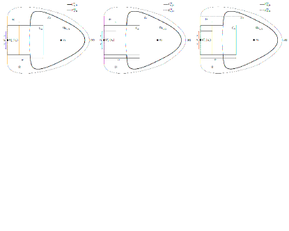
Figure 6: A schematic representation of $\mathsf{V}_{4\varepsilon}^{r}(z_{k})$.

For each $z\in\overline{\Gamma_{k,\mathbf{D}}^{\textsc{M}}}$, recall that $x^{\prime}=(x_{1},\ldots,x_{d-1})$ is a system of coordinates defined in a neighborhood of $z$ in $\partial\Omega$ such that (131), (132), and (133) hold. Recall that $x\mapsto(\mathsf{z}(x),x_{d}(x))$ introduced in (105) and (129) defines a $\mathcal{C}^{\infty}$ diffeomorphism on $\{x\in\overline{\Omega},x_{d}(x)\in[0,3\varepsilon)\}$. To ease the notation, from now on, we simply write $\{x_{d}\in\mathsf{O}\}$ for the set $\{x\in\overline{\Omega},x_{d}(x)\in\mathsf{O}\}$ for $\mathsf{O}\subset\mathbb{R}_{+}$. Recall that by (106) and since $\mathsf{n}_{\mathsf{M}}(z_{k})$ is an eigenvector of ${\rm Hess\,}f(z_{k})$ for the eigenvalue $\mu_{z_{k}}<0$, up to choosing $\varepsilon>0$ and $r>0$ smaller,

$$\forall x=(x^{\prime},x_{d})\in\mathsf{V}_{4\varepsilon}^{r}(z_{k}),\ f(x)\ =\ f(0)+\frac{1}{2}x^{\prime}\cdot\text{Hess}f|_{\partial\Omega}(z_{k})x^{\prime}-\frac{|\mu_{z_{k}}|}{2}x_{d}^{2}+O(|x|^{3}).$$ (190)

Since $\text{Hess}f|_{\partial\Omega}(z_{k})$ is positive-definite, we may assume in the following that $r>0$ and $\varepsilon>0$ are small enough such that

$$\{z_{k}\}=\operatorname*{arg\,min}_{{\mathsf{V}_{4\varepsilon}^{r}(z_{k})}}(f+|\mu_{z_{k}}|x_{d}^{2}).$$ (191)

Moreover, because $\overline{\Gamma_{k,\mathbf{D}}^{\textsc{M}}}\subset\Gamma_{z_{k}}$ and $\Gamma_{z_{k}}\subset\mathsf{W}_{+}^{z_{k}}$ (see (14)), one has $\{z_{k}\}=\operatorname*{arg\,min}_{\overline{\Gamma_{k,\mathbf{D}}^{\textsc{M}}}}f.$ With a slight abuse of notation, we still denote by $f$ the function $f$ in the $(\mathsf{z},x_{d})$ variable. Since $f(\mathsf{z},x_{d})=f(\mathsf{z},0)+o_{\varepsilon}(1)$ uniformly on $x=(\mathsf{z},x_{d})\in\overline{\mathsf{C}_{4\varepsilon}}$ as $\varepsilon\to 0$, it thus holds if in addition $\mathsf{z}\in\overline{\Gamma_{k,\mathbf{D}}^{\textsc{M}}}\setminus\overline{\mathsf{B}_{\partial\Omega}(z_{k},r)}$, $f(\mathsf{z},x_{d})\geq f(z_{k})+c-o_{\varepsilon}(1)$ for some $c>0$ independant of $x_{d}\in[0,4\varepsilon]$. This implies that up to choosing $\varepsilon>0$ smaller, it holds for some $c>0$,

$$f>f(z_{k})+c/2\ \text{on}\ \overline{\mathsf{C}_{4\varepsilon}}\setminus\mathsf{V}_{4\varepsilon}^{r}(z_{k})=\{x=(\mathsf{z},x_{d}),\mathsf{z}\in\overline{\Gamma_{k,\mathbf{D}}^{\textsc{M}}}\setminus\overline{\mathsf{B}_{\partial\Omega}(z_{k},r)},x_{d}\in[0,4\varepsilon]\}.$$ (192)

Let us consider $\chi\in\mathcal{C}^{\infty}(\mathbb{R}_{+},[0,1])$ such that $\text{supp }\chi\subset[0,\varepsilon]\,\text{ and }\,\chi=1\text{ on }[0,\varepsilon/2].$ Inspired by [9] (see also [58, Section 4.2] and [24]), we build a quasi-mode for $\Delta_{f,h}^{\textsc{M},(0)}(\mathsf{\Omega}_{k}^{\textsc{M}})$ using the function $\phi_{k}^{\textsc{M},(0)}$ defined on $\overline{\mathsf{C}_{\alpha}}\cap\{x_{d}\in[0,2\varepsilon]\}=\overline{\mathsf{C}_{2\varepsilon}}$ (see (135)) by:

$$\forall x=(\mathsf{z},x_{d})\in\overline{\mathsf{C}_{2\varepsilon}},\ \ \phi^{\textsc{M},(0)}_{k}(\mathsf{z},x_{d}):=\frac{\int_{0}^{x_{d}}\chi(t)e^{-\frac{1}{h}|\mu_{z_{k}}|\,t^{2}}dt}{\int_{0}^{2\varepsilon}\chi(t)\,e^{-\frac{1}{h}|\mu_{z_{k}}|\,t^{2}}dt}.$$ (193)

Notice that the function $\phi^{\textsc{M},(0)}_{k}$ only depends on the variable $x_{d}$. Moreover, one has:

$$\phi^{\textsc{M},(0)}_{k}\in\mathcal{C}^{\infty}\big{(}\overline{\mathsf{C}_{2\varepsilon}}\big{)}\text{ and }\forall x=(\mathsf{z},x_{d})\in\overline{\mathsf{C}_{2\varepsilon}},\,\phi^{\textsc{M},(0)}_{k}(x)=1\text{ if }x_{d}\in[\varepsilon,2\varepsilon].$$

Let us set for $x=(\mathsf{z},x_{d})\in\overline{\mathsf{C}_{2\varepsilon}}$:

$$\psi^{\textsc{M},(0)}_{k}(x)=\phi^{\textsc{M},(0)}_{k}(\mathsf{z},x_{d}).$$ (194)

We extend $\psi^{\textsc{M},(0)}_{k}$ from $\overline{\mathsf{C}_{2\varepsilon}}=\overline{\mathsf{\Omega}_{k}^{\textsc{M}}}\cap\{x_{d}\in[0,2\varepsilon]\}$ (see (187)) to $\overline{\mathsf{\Omega}_{k}^{\textsc{M}}}$ by setting $\psi^{\textsc{M},(0)}_{k}=1\text{ on }\overline{\mathsf{\Omega}_{k}^{\textsc{M}}}\cap\{x_{d}>2\varepsilon\}=\overline{\mathsf{\Omega}_{k}^{\textsc{M}}}\setminus\overline{\mathsf{C}_{2\varepsilon}}.$ One then has $\psi^{\textsc{M},(0)}_{k}\in\mathcal{C}^{\infty}\big{(}\overline{\mathsf{\Omega}_{k}^{\textsc{M}}}\big{)}$. Notice that from (188),

$$\psi^{\textsc{M},(0)}_{k}=1\text{ in a neighborhood of $x_{0}$ in $\mathsf{\Omega}_{k}^{\textsc{M}}$}.$$ (195)

Then, define on $\overline{\mathsf{\Omega}_{k}^{\textsc{M}}}$:

$$\varphi^{\textsc{M},(0)}_{k}=\frac{\psi^{\textsc{M},(0)}_{k}\,e^{-\frac{1}{h}f}}{\|\psi^{\textsc{M},(0)}_{k}\,e^{-\frac{1}{h}f}\|_{L^{2}(\mathsf{\Omega}_{k}^{\textsc{M}})}}\in\mathcal{C}^{\infty}\big{(}\overline{\mathsf{\Omega}_{k}^{\textsc{M}}}\big{)}.$$ (196)

Let us check that $\varphi^{\textsc{M},(0)}_{k}$ belongs to the domain of $\Delta_{f,h}^{\textsc{M},(0)}(\mathsf{\Omega}_{k}^{\textsc{M}})$, defined in (178). Because it is smooth on the bounded set $\overline{\mathsf{\Omega}_{k}^{\textsc{M}}}$, one just has to check that it satisfies the boundary conditions on $\partial\mathsf{\Omega}_{k}^{\textsc{M}}$. By definition of $\phi^{\textsc{M},(0)}_{k}$ above, $\varphi^{\textsc{M},(0)}_{k}(x)=0$ for all $x=(\mathsf{z},x_{d})\in\overline{\mathsf{C}_{2\varepsilon}}\cap\{x_{d}=0\}=\overline{\Gamma_{k,\mathbf{D}}^{\textsc{M}}}$ (see (135)). Let us now check that $\partial_{\mathsf{n}_{\mathsf{\Omega}_{k}^{\textsc{M}}}}(e^{\frac{f}{h}}\varphi^{\textsc{M},(0)}_{k})(x)=0$ for a.e. $x\in\Gamma_{k,\mathbf{N}}^{\textsc{M}}$, i.e. that $\partial_{\mathsf{n}_{\mathsf{\Omega}_{k}^{\textsc{M}}}}\psi^{\textsc{M},(0)}_{k}(x)=0$ for a.e. $x\in\Gamma_{k,\mathbf{N}}^{\textsc{M}}$. Recall that $\Gamma_{k,\mathbf{N}}^{\textsc{M}}=\partial\mathsf{\Omega}_{k}^{\textsc{M}}\cap\Omega$ (see (147)). Let us first consider the case $x\in\Gamma_{k,\mathbf{N}}^{\textsc{M}}\cap\{x_{d}\in(0,3\varepsilon)\}$. From (187) and (138), it holds:

$$\partial\mathsf{\Omega}_{k}^{\textsc{M}}\cap\{x_{d}\in(0,3\varepsilon)\}=\Sigma_{3\varepsilon}^{lateral}.$$ (197)

Because $\overline{\Omega_{\mathsf{K}_{\alpha/2}}}\subset\{x_{d}>5\varepsilon\}$ and $\Sigma_{3\varepsilon}^{lateral}\subset\partial\mathsf{C}_{\alpha}$, one deduces that (see (150) and (151)),

$$\Sigma_{3\varepsilon}^{lateral}=\Gamma_{k,\mathbf{N}}^{\textsc{M}}\cap\{x_{d}\in(0,3\varepsilon)\}\subset\mathsf{A}_{2}.$$

Then using (154) and (140), $\mathsf{n}_{\mathsf{\Omega}_{k}^{\textsc{M}}}=-{\nabla x_{1}}/{|\nabla x_{1}|}$ on $\Sigma_{3\varepsilon}^{lateral}$. Since $\nabla\psi^{\textsc{M},(0)}_{k}$ is collinear to $\nabla x_{d}$ on $\overline{\mathsf{C}_{3\varepsilon}}$ which is, in view of (106), orthogonal to $\nabla x_{1}$, it holds:

$$\partial_{\mathsf{n}_{\mathsf{\Omega}_{k}^{\textsc{M}}}}\psi^{\textsc{M},(0)}_{k}(x)=0\text{ for }x\in\Gamma_{k,\mathbf{N}}^{\textsc{M}}\cap\Sigma_{3\varepsilon}^{lateral}.$$

Let us now consider the case $x\in\Gamma_{k,\mathbf{N}}^{\textsc{M}}\cap\{x_{d}\geq 3\varepsilon\}$. Because $\psi^{\textsc{M},(0)}_{k}=1$ on $\overline{\mathsf{\Omega}_{k}^{\textsc{M}}}\setminus\overline{\mathsf{C}_{\varepsilon}}=\overline{\mathsf{\Omega}_{k}^{\textsc{M}}}\cap\{x_{d}>\varepsilon\}$ (therefore $|\nabla\psi^{\textsc{M},(0)}_{k}|(x)=0$ on this set) and $\Gamma_{k,\mathbf{N}}^{\textsc{M}}\cap\{x_{d}\geq 3\varepsilon\}=\partial\mathsf{\Omega}_{k}^{\textsc{M}}\cap\{x_{d}\geq 3\varepsilon\}$, it holds,

$$\partial_{\mathsf{n}_{\mathsf{\Omega}_{k}^{\textsc{M}}}}\psi^{\textsc{M},(0)}_{k}(x)=0\text{ for a.e. }x\in\Gamma_{k,\mathbf{N}}^{\textsc{M}}\cap\{x_{d}\geq 3\varepsilon\}.$$

In conclusion, one has

$$\varphi^{\textsc{M},(0)}_{k}\in\mathcal{D}(\Delta_{f,h}^{\textsc{M},(0)}(\mathsf{\Omega}_{k}^{\textsc{M}})).$$ (198)

Step 2: Asymptotic estimates of $\langle\varphi^{\textsc{M},(0)}_{k},\Delta_{f,h}^{\textsc{M},(0)}(\mathsf{\Omega}_{k}^{\textsc{M}})\varphi^{\textsc{M},(0)}_{k}\rangle_{L^{2}(\mathsf{\Omega}_{k}^{\textsc{M}})}$ and $\|\Delta_{f,h}^{\textsc{M},(0)}(\mathsf{\Omega}_{k}^{\textsc{M}})\varphi^{\textsc{M},(0)}_{k}\|_{L^{2}(\mathsf{\Omega}_{k}^{\textsc{M}})}^{2}$ as $h\to 0$. Let us first deal with $\mathsf{Z}_{z_{k}}:=\|\psi^{\textsc{M},(0)}_{k}\,e^{-\frac{1}{h}f}\|_{L^{2}(\mathsf{\Omega}_{k}^{\textsc{M}})}$. Because $|\psi^{\textsc{M},(0)}_{k}|\leq 1$, $\{x_{0}\}=\operatorname*{arg\,min}_{\overline{\mathsf{\Omega}_{k}^{\textsc{M}}}}f$ (which follows from the fact that $x_{0}\in\mathsf{\Omega}_{k}^{\textsc{M}}\subset\Omega$ and Lemma 4) and $\psi^{\textsc{M},(0)}_{k}=1$ near $x_{0}$ in $\mathsf{\Omega}_{k}^{\textsc{M}}$ (see (195)) it holds, using Laplace’s method, in the limit $h\to 0$:

$$\mathsf{Z}_{z_{k}}=\sqrt{\kappa_{x_{0}}}\,h^{\frac{d}{4}}\,e^{-\frac{1}{h}f(x_{0})}\big{(}1+O(h)\big{)},$$ (199)

where $\kappa_{x_{0}}$ is defined in (186). Let us now consider the term $\langle\varphi^{\textsc{M},(0)}_{k},\Delta_{f,h}^{\textsc{M},(0)}(\mathsf{\Omega}_{k}^{\textsc{M}})\varphi^{\textsc{M},(0)}_{k}\rangle_{L^{2}(\mathsf{\Omega}_{k}^{\textsc{M}})}$. One has (see (198) and Proposition 33):

$$\langle\varphi^{\textsc{M},(0)}_{k},\Delta_{f,h}^{\textsc{M},(0)}(\mathsf{\Omega}_{k}^{\textsc{M}})\varphi^{\textsc{M},(0)}_{k}\rangle_{L^{2}(\mathsf{\Omega}_{k}^{\textsc{M}})}=\int_{\mathsf{\Omega}_{k}^{\textsc{M}}}|\mathsf{d}_{f,h}\varphi^{\textsc{M},(0)}_{k}|^{2}=\frac{h^{2}\int_{\mathsf{C}_{2\varepsilon}}|\nabla\psi^{\textsc{M},(0)}_{k}|^{2}e^{-\frac{2}{h}f}}{\mathsf{Z}_{z_{k}}^{2}}$$

where we also used the fact that $\psi^{\textsc{M},(0)}_{k}=1$ on $\overline{\mathsf{\Omega}_{k}^{\textsc{M}}}\setminus\overline{\mathsf{C}_{2\varepsilon}}$. For $\eta\in[0,2\varepsilon]$, set $\Gamma(\eta)=\{x\in\overline{\mathsf{C}_{2\varepsilon}},x_{d}(x)=\eta\}$. Note that $\Gamma(0)=\Gamma^{\textsc{M}}_{k,\mathbf{D}}$ and that for any $\eta\in[0,2\varepsilon]$, $\Gamma(\eta)$ is naturally parametrized by $\Gamma^{\textsc{M}}_{k,\mathbf{D}}$ through the mapping $\mathsf{z}\in\Gamma^{\textsc{M}}_{k,\mathbf{D}}\mapsto(\mathsf{z},\eta)$ with Jacobian determinant $\mathsf{j}(\mathsf{z},\eta)$ with $\mathsf{j}(\mathsf{z},0)=1$. One has using (194), (193), the co-area formula [31] ($dx=d\sigma_{\Gamma(\eta)}|\nabla x_{d}|^{-1}d\eta$), and the fact that $|\nabla x_{d}|=1$:

$${h^{2}\int_{\mathsf{C}_{2\varepsilon}}|\nabla\psi^{\textsc{M},(0)}_{k}|^{2}e^{-\frac{2}{h}f}} =\frac{\int_{\eta=0}^{2\varepsilon}\chi^{2}(\eta)\int_{\Gamma(\eta)}|\nabla x_{d}|^{2}\,e^{-\frac{2}{h}(f+|\mu_{z_{k}}|\eta^{2})}d\sigma_{\Gamma(\eta)}|\nabla x_{d}|^{-1}d\eta}{\Big{(}\int_{0}^{2\varepsilon}\chi(t)\,e^{-\frac{1}{h}|\mu_{z_{k}}|\,t^{2}}dt\Big{)}^{2}}$$

$$=\frac{\int_{\eta=0}^{2\varepsilon}\chi^{2}(\eta)\int_{\mathsf{z}\in\Gamma_{k,\mathbf{D}}^{\textsc{M}}}e^{-\frac{2}{h}(f(\mathsf{z},\eta)+|\mu_{z_{k}}|\eta^{2})}\mathsf{j}(\mathsf{z},\eta)d\sigma_{\Gamma^{\textsc{M}}_{k,\mathbf{D}}}d\eta}{\Big{(}\int_{0}^{2\varepsilon}\chi(t)\,e^{-\frac{1}{h}|\mu_{z_{k}}|\,t^{2}}dt\Big{)}^{2}}.$$

A straightforward computation implies that there exists $c>0$ such that in the limit $h\to 0$,

$$\mathsf{N}_{z_{k}}:=\int_{0}^{2\varepsilon}\chi(t)\,e^{-\frac{1}{h}|\mu_{z_{k}}|\,t^{2}}dt=\frac{\sqrt{\pi h}}{2\sqrt{|\mu_{z_{k}}|}}\big{(}1+O(e^{-\frac{c}{h}})\big{)}.$$ (200)

Using (192) and (189), one has for $h$ small enough:

$$\int_{\eta=0}^{2\varepsilon}\chi^{2}(\eta)\int_{\mathsf{z}\in\Gamma_{k,\mathbf{D}}^{\textsc{M}}}\!\!\!\!e^{-\frac{2}{h}(f(\mathsf{z},\eta)+|\mu_{z_{k}}|\eta^{2})}\mathsf{j}(\mathsf{z},\eta)d\sigma_{\Gamma^{\textsc{M}}_{k,\mathbf{D}}}d\eta =\int_{\eta=0}^{2\varepsilon}\chi^{2}(\eta)\int_{|\mathsf{z}|\leq r}\!\!\!\!e^{-\frac{2}{h}(f(\mathsf{z},\eta)+|\mu_{z_{k}}|\eta^{2})}\mathsf{j}(\mathsf{z},\eta)d\sigma_{\Gamma^{\textsc{M}}_{k,\mathbf{D}}}d\eta$$

$$\quad+O(e^{-\frac{2}{h}(f(z_{k})+c)}),$$

for some $c>0$ independent of $h$. Using in addition (190), the same computations as in the proof of the step 1.b of [58, Proposition 24] imply that in the limit $h\to 0$:

$$\int_{\eta=0}^{2\varepsilon}\chi^{2}(\eta)\int_{|\mathsf{z}|\leq r}\!\!\!\!e^{-\frac{2}{h}(f(\mathsf{z},\eta)+|\mu_{z_{k}}|\eta^{2})}\mathsf{j}(\mathsf{z},\eta)d\sigma_{\Gamma^{\textsc{M}}_{k,\mathbf{D}}}d\eta=\frac{(\pi h)^{\frac{d}{2}}e^{-\frac{2}{h}f(z_{k})}}{2\sqrt{\mu_{1}\cdots\mu_{d-1}|\mu_{z_{k}}|}}\big{(}1+O(\sqrt{h})\big{)},$$

where the $O(\sqrt{h})$ is optimal in general. In conclusion, using also (199), one has as $h\to 0$:

$$\langle\varphi^{\textsc{M},(0)}_{k},\Delta_{f,h}^{\textsc{M},(0)}(\mathsf{\Omega}_{k}^{\textsc{M}})\varphi^{\textsc{M},(0)}_{k}\rangle_{L^{2}(\mathsf{\Omega}_{k}^{\textsc{M}})}=\mathsf{A}_{x_{0},z_{k}}h\ e^{-\frac{2}{h}(f(z_{k})-f(x_{0}))}(1+O(\sqrt{h})).$$ (201)

Let us now consider the term $\|\Delta_{f,h}^{\textsc{M},(0)}(\mathsf{\Omega}_{k}^{\textsc{M}})\varphi^{\textsc{M},(0)}_{k}\|_{L^{2}(\mathsf{\Omega}_{k}^{\textsc{M}})}^{2}$. Using (118) and the definition of $\psi^{\textsc{M},(0)}_{k}$, it holds on $\mathsf{\Omega}_{k}^{\textsc{M}}$:

$$\Delta_{f,h}^{(0)}\varphi^{\textsc{M},(0)}_{k} =\frac{2he^{-\frac{1}{h}f}}{\|\psi^{\textsc{M},(0)}_{k}\,e^{-\frac{1}{h}f}\|_{L^{2}(\mathsf{\Omega}_{k}^{\textsc{M}})}}\Big{(}\,\frac{h}{2}\Delta_{\mathbf{H}}^{(0)}+\nabla f\cdot\nabla\,\Big{)}\psi^{\textsc{M},(0)}_{k}\ \text{ is supported in $\overline{\mathsf{C}_{2\varepsilon}}$.}$$ (202)

By (194), (200), and (193), for $h$ small enough, $\|\Delta_{\mathbf{H}}^{(0)}\psi^{\textsc{M},(0)}_{k}\|_{L^{\infty}(\mathsf{C}_{2\varepsilon})}$ and $\|\nabla\psi^{\textsc{M},(0)}_{k}\|_{L^{\infty}(\mathsf{C}_{2\varepsilon})}$ are $O(h^{\nu})$ for some $\nu\in\mathbb{R}$. Then, using (192) and (199), one has for $h$ small enough (see (189)):

$$\|\Delta_{f,h}^{\textsc{M},(0)}(\mathsf{\Omega}_{k}^{\textsc{M}})\varphi^{\textsc{M},(0)}_{k}\|_{L^{2}(\mathsf{\Omega}_{k}^{\textsc{M}})}^{2} =\|\Delta_{f,h}^{\textsc{M},(0)}(\mathsf{\Omega}_{k}^{\textsc{M}})\varphi^{\textsc{M},(0)}_{k}\|_{L^{2}(\mathsf{C}_{2\varepsilon})}^{2}$$

$$=\|\Delta_{f,h}^{\textsc{M},(0)}(\mathsf{\Omega}_{k}^{\textsc{M}})\varphi^{\textsc{M},(0)}_{k}\|_{L^{2}(\mathsf{V}_{2\varepsilon}^{r}(z_{k}))}^{2}+O(e^{-\frac{2}{h}(f(z_{k})-f(x_{0})+c)}),$$ (203)

for some $c>0$ independent of $h$. Let us recall that $\mathbf{g}$ denotes the metric tensor in the $(x^{\prime},x_{d})$ coordinates (see (106)). In the following, with a slight abuse of notation, we also denote by $\mathbf{g}$ the matrix $(\mathbf{G},0;0,1)$. In the $(x^{\prime},x_{d})$-coordinates, $\Delta_{\mathbf{H}}^{(0)}$ writes

$$\Delta_{\mathbf{H}}^{(0)}\phi^{\textsc{M},(0)}_{k}=-\frac{1}{\sqrt{|\mathbf{g}|}}\sum_{i,j=1}^{d}\partial_{x_{i}}\big{(}\sqrt{|\mathbf{g}|}\,\mathbf{g}^{i,j}\partial_{x_{j}}\phi^{\textsc{M},(0)}_{k}\big{)},$$

where $|\mathbf{g}|$ denotes the determinant of $\mathbf{g}$ and $\mathbf{g}^{i,j}$ the $(i,j)$ entry of $\mathbf{g}^{-1}$. Then, from (202) and (193), one has on $\mathsf{V}_{2\varepsilon}^{r}(z_{k})$,

$$\Delta_{f,h}\varphi^{\textsc{M},(0)}_{k} =\frac{2h\,e^{-\frac{f}{h}}}{\mathsf{Z}_{z_{k}}}\Big{[}-\frac{h}{2\sqrt{|\mathbf{g}|}}\sum_{i,j=1}^{d}\partial_{x_{i}}\big{(}\sqrt{|\mathbf{g}|}\,\mathbf{g}^{i,j}\partial_{x_{j}}\phi^{\textsc{M},(0)}_{k}\big{)}+\,\sum_{i,j=1}^{d}\mathbf{g}^{i,j}\partial_{x_{i}}f\partial_{x_{j}}\phi^{\textsc{M},(0)}_{k}\,\Big{]}$$

$$=\frac{2h\,e^{-\frac{1}{h}(f+|\mu_{z_{k}}|x_{d}^{2})}}{\mathsf{Z}_{z_{k}}\mathsf{N}_{z_{k}}}\Big{[}-\frac{h}{2\sqrt{|\mathbf{g}|}}\sum_{i=1}^{d}\partial_{x_{i}}\big{(}\sqrt{|\mathbf{g}|}\,\mathbf{g}^{i,d}\big{)}\chi(x_{d})+\mathbf{g}^{d,d}\chi(x_{d})|\mu_{z_{k}}|x_{d}$$

$$\qquad\qquad\qquad\qquad\qquad+\chi(x_{d})\sum_{i=1}^{d}\mathbf{g}^{i,d}\partial_{x_{i}}f-\frac{h}{2}\,\chi^{\prime}(x_{d})\,\mathbf{g}^{d,d}\Big{]}$$

$$=\frac{2h\,e^{-\frac{1}{h}(f+|\mu_{z_{k}}|x_{d}^{2})}}{\mathsf{Z}_{z_{k}}\mathsf{N}_{z_{k}}}\big{[}O(h)+O(|x|^{2})\big{]},$$

where $\mathsf{N}_{z_{k}}$ is defined in (200), and where in the last inequality we have used that $\mathbf{g}^{i,d}=0$ for $i=1,\ldots,d-1$ (see (106)), and $\partial_{x_{d}}f(x^{\prime},x_{d})=-|\mu_{z_{k}}|x_{d}+O(|x|^{2})$ (see (190)). Notice the cancelation of the $O(x)$ terms in the previous computations due to the precise form of the quasi-mode $\varphi^{\textsc{M},(0)}_{k}$. Thus, by (191), (199), (190), (200), and (201), one deduces using Laplace’s method that as $h\to 0$,

$$\|\Delta_{f,h}^{\textsc{M},(0)}(\mathsf{\Omega}_{k}^{\textsc{M}})\varphi^{\textsc{M},(0)}_{k}\|_{L^{2}(\mathsf{V}_{\varepsilon}^{r}(z_{k}))}^{2} =\frac{h^{2}h^{\frac{d}{2}}}{h^{\frac{d}{2}}h}\,O(h^{2})\,e^{-\frac{2}{h}(f(z_{k})-f(x_{0}))}$$

$$=O(h^{2})|\langle\varphi^{\textsc{M},(0)}_{k},\Delta_{f,h}^{\textsc{M},(0)}(\mathsf{\Omega}_{k}^{\textsc{M}})\varphi^{\textsc{M},(0)}_{k}\rangle_{L^{2}(\mathsf{\Omega}_{k}^{\textsc{M}})}|.$$

Consequently, one deduces using (203), that

$$\|\Delta_{f,h}^{\textsc{M},(0)}(\mathsf{\Omega}_{k}^{\textsc{M}})\varphi^{\textsc{M},(0)}_{k}\|_{L^{2}(\mathsf{\Omega}_{k}^{\textsc{M}})}=O(h)\sqrt{|\langle\varphi^{\textsc{M},(0)}_{k},\Delta_{f,h}^{\textsc{M},(0)}(\mathsf{\Omega}_{k}^{\textsc{M}})\varphi^{\textsc{M},(0)}_{k}\rangle_{L^{2}(\mathsf{\Omega}_{k}^{\textsc{M}})}|}.$$ (204)

Step 3: End of the proof of Proposition 36. Let us introduce the constant $\mathsf{c}>0$ from item $(iii)$ in Proposition 35. Because $\varphi^{\textsc{M},(0)}_{k}\in\mathcal{D}(\Delta_{f,h}^{\textsc{M},(0)}(\mathsf{\Omega}_{k}^{\textsc{M}}))$, see indeed (198), and since $\lambda(\mathsf{\Omega}_{k}^{\textsc{M}})$ is exponentially small when $h\to 0$ (actually $o(h)$ as $h\to 0$ would be enough), using the fact that (see the proof of [58, Proposition 27])

$$(1-\pi_{[0,\mathsf{c}h]}\big{(}\Delta_{f,h}^{\textsc{M},(0)}(\mathsf{\Omega}_{k}^{\textsc{M}})\big{)})\,\varphi^{\textsc{M},(0)}_{k}=-\frac{1}{2\pi i}\int_{C(\mathsf{c}h/2)}z^{-1}(z-\Delta_{f,h}^{\textsc{M},(0)})^{-1}\Delta_{f,h}^{\textsc{M},(0)}\varphi^{\textsc{M},(0)}_{k}dz,$$

where $C(\mathsf{c}h/2)\subset\mathbb{C}$ is the circle of radius $\mathsf{c}h/2$ centered at $0$, it holds for $h$ small enough

$$\|(1-\pi_{[0,\mathsf{c}h]}\big{(}\Delta_{f,h}^{\textsc{M},(0)}(\mathsf{\Omega}_{k}^{\textsc{M}})\big{)})\,\varphi^{\textsc{M},(0)}_{k}\|_{L^{2}(\mathsf{\Omega}_{k}^{\textsc{M}})}\leq Ch^{-1}\|\Delta_{f,h}^{\textsc{M},(0)}(\mathsf{\Omega}_{k}^{\textsc{M}})\varphi^{\textsc{M},(0)}_{k}\|_{L^{2}(\mathsf{\Omega}_{k}^{\textsc{M}})}.$$

Therefore, using (204), it holds:

$$\|(1-\pi_{[0,\mathsf{c}h]}\big{(}\Delta_{f,h}^{\textsc{M},(0)}(\mathsf{\Omega}_{k}^{\textsc{M}})\big{)})\,\varphi^{\textsc{M},(0)}_{k}\|_{L^{2}(\mathsf{\Omega}_{k}^{\textsc{M}})}\leq C\sqrt{|\langle\varphi^{\textsc{M},(0)}_{k},\Delta_{f,h}^{\textsc{M},(0)}(\mathsf{\Omega}_{k}^{\textsc{M}})\varphi^{\textsc{M},(0)}_{k}\rangle_{L^{2}(\mathsf{\Omega}_{k}^{\textsc{M}})}|}.$$ (205)

In particular, using (201) and the fact that $\|\varphi^{\textsc{M},(0)}_{k}\|_{L^{2}(\mathsf{\Omega}_{k}^{\textsc{M}})}=1$, there exists $c>0$ (because $f(z_{k})>f(x_{0})$ see Lemma 4) such that, for $h>0$ small enough,

$$\|\pi_{[0,\mathsf{c}h]}\big{(}\Delta_{f,h}^{\textsc{M},(0)}(\mathsf{\Omega}_{k}^{\textsc{M}})\big{)}\varphi^{\textsc{M},(0)}_{k}\|_{L^{2}(\mathsf{\Omega}_{k}^{\textsc{M}})}=1+O(e^{-\frac{c}{h}}),$$ (206)

and the following function is therefore well defined :

$$\mathsf{u}^{(0)}_{k}=\frac{\pi_{[0,\mathsf{c}h]}\big{(}\Delta_{f,h}^{\textsc{M},(0)}(\mathsf{\Omega}_{k}^{\textsc{M}})\big{)}\varphi^{\textsc{M},(0)}_{k}}{\|\pi_{[0,\mathsf{c}h]}\big{(}\Delta_{f,h}^{\textsc{M},(0)}(\mathsf{\Omega}_{k}^{\textsc{M}})\big{)}\varphi^{\textsc{M},(0)}_{k}\|_{L^{2}(\mathsf{\Omega}_{k}^{\textsc{M}})}}.$$ (207)

One has

$$\lambda(\mathsf{\Omega}_{k}^{\textsc{M}}) =\langle\mathsf{u}^{(0)}_{k},\Delta_{f,h}^{\textsc{M},(0)}(\mathsf{\Omega}_{k}^{\textsc{M}})\mathsf{u}^{(0)}_{k}\big{\rangle}_{L^{2}(\mathsf{\Omega}_{k}^{\textsc{M}})}$$ (208)

$$=\langle\pi_{[0,\mathsf{c}h]}\big{(}\Delta_{f,h}^{\textsc{M},(0)}(\mathsf{\Omega}_{k}^{\textsc{M}})\big{)}\varphi^{\textsc{M},(0)}_{k},\Delta_{f,h}^{\textsc{M},(0)}(\mathsf{\Omega}_{k}^{\textsc{M}})\varphi^{\textsc{M},(0)}_{k}\big{\rangle}_{L^{2}(\mathsf{\Omega}_{k}^{\textsc{M}})}(1+O(e^{-\frac{c}{h}})),$$

since the orthogonal projector $\pi_{[0,\mathsf{c}h]}\big{(}\Delta_{f,h}^{\textsc{M},(0)}(\mathsf{\Omega}_{k}^{\textsc{M}})\big{)}$ and $\Delta_{f,h}^{\textsc{M},(0)}(\mathsf{\Omega}_{k}^{\textsc{M}})$ commute on $\mathcal{D}(\Delta_{f,h}^{\textsc{M},(0)}(\mathsf{\Omega}_{k}^{\textsc{M}}))$ and $\varphi^{\textsc{M},(0)}_{k}\in\mathcal{D}(\Delta_{f,h}^{\textsc{M},(0)}(\mathsf{\Omega}_{k}^{\textsc{M}}))$. In addition, one has using (205) and (204),

$$\langle\pi_{[0,\mathsf{c}h]}\big{(}\Delta_{f,h}^{\textsc{M},(0)}(\mathsf{\Omega}_{k}^{\textsc{M}})\big{)}\varphi^{\textsc{M},(0)}_{k},\Delta_{f,h}^{\textsc{M},(0)}(\mathsf{\Omega}_{k}^{\textsc{M}})\varphi^{\textsc{M},(0)}_{k}\big{\rangle}_{L^{2}(\mathsf{\Omega}_{k}^{\textsc{M}})}$$

$$=\langle\varphi^{\textsc{M},(0)}_{k},\Delta_{f,h}^{\textsc{M},(0)}(\mathsf{\Omega}_{k}^{\textsc{M}})\varphi^{\textsc{M},(0)}_{k}\big{\rangle}_{L^{2}(\mathsf{\Omega}_{k}^{\textsc{M}})}-\langle(1-\pi_{[0,\mathsf{c}h]}\big{(}\Delta_{f,h}^{\textsc{M},(0)}(\mathsf{\Omega}_{k}^{\textsc{M}})\big{)})\varphi^{\textsc{M},(0)}_{k},\Delta_{f,h}^{\textsc{M},(0)}(\mathsf{\Omega}_{k}^{\textsc{M}})\varphi^{\textsc{M},(0)}_{k}\big{\rangle}_{L^{2}(\mathsf{\Omega}_{k}^{\textsc{M}})}$$

$$=\langle\varphi^{\textsc{M},(0)}_{k},\Delta_{f,h}^{\textsc{M},(0)}(\mathsf{\Omega}_{k}^{\textsc{M}})\varphi^{\textsc{M},(0)}_{k}\big{\rangle}_{L^{2}(\mathsf{\Omega}_{k}^{\textsc{M}})}(1+O(h)),$$

$$=\mathsf{A}_{x_{0},z_{k}}h\ e^{-\frac{2}{h}(f(z_{k})-f(x_{0}))}(1+O(\sqrt{h})).$$

where we used (201). This proves  (183). It remains to prove Equation (185).

Let $\mathsf{u}^{(1)}_{k}$ be a $L^{2}(\mathsf{\Omega}_{k}^{\textsc{M}})$-normalized eigenform of $\Delta_{f,h}^{\textsc{M},(1)}(\mathsf{\Omega}_{k}^{\textsc{M}})$ associated with the eigenvalue $\lambda(\mathsf{\Omega}_{k}^{\textsc{M}})$. In view of item $(ii)$ and $(iii)$ in Proposition 35 it holds ($\mathsf{u}^{(0)}_{k}$ is indeed a $L^{2}(\mathsf{\Omega}_{k}^{\textsc{M}})$-normalized principal eigenform of $\Delta_{f,h}^{\textsc{M},(0)}(\mathsf{\Omega}_{k}^{\textsc{M}})$, see (207)), $\mathsf{u}^{(1)}_{k}=\pm\mathsf{d}_{f,h}\mathsf{u}^{(0)}_{k}/\|\mathsf{d}_{f,h}\mathsf{u}^{(0)}_{k}\|_{L^{2}(\mathsf{\Omega}_{k}^{\textsc{M}})}$. Let us choose

$$\mathsf{u}^{(1)}_{k}=\frac{\mathsf{d}_{f,h}\mathsf{u}^{(0)}_{k}}{\mathsf{N}_{k}^{(1)}}\text{ with }\mathsf{N}_{k}^{(1)}=\big{\|}\mathsf{d}_{f,h}\mathsf{u}^{(0)}_{k}\big{\|}_{L^{2}(\mathsf{\Omega}_{k}^{\textsc{M}})}.$$ (209)

From (208), one has, $\lambda(\mathsf{\Omega}_{k}^{\textsc{M}})=\langle\mathsf{d}_{f,h}\mathsf{u}^{(0)}_{k},\mathsf{d}_{f,h}\mathsf{u}^{(0)}_{k}\big{\rangle}_{L^{2}(\mathsf{\Omega}_{k}^{\textsc{M}})}=(\mathsf{N}_{k}^{(1)})^{2}$, and thus, using (207) and the fact that $\mathsf{d}_{f,h}\pi_{[0,\mathsf{c}h]}\big{(}\Delta_{f,h}^{\textsc{M},(0)}(\mathsf{\Omega}_{k}^{\textsc{M}})\big{)}=\pi_{[0,\mathsf{c}h]}\big{(}\Delta_{f,h}^{\textsc{M},(1)}(\mathsf{\Omega}_{k}^{\textsc{M}})\big{)}\mathsf{d}_{f,h}$ (see item $(ii)$ in Proposition 35),

$$\lambda(\mathsf{\Omega}_{k}^{\textsc{M}}) =\frac{\mathsf{N}_{k}^{(1)}\,\langle\mathsf{d}_{f,h}\varphi^{\textsc{M},(0)}_{k},\mathsf{u}^{(1)}_{k}\big{\rangle}_{L^{2}(\mathsf{\Omega}_{k}^{\textsc{M}})}}{\|\pi_{[0,\mathsf{c}h]}\big{(}\Delta_{f,h}^{\textsc{M},(0)}(\mathsf{\Omega}_{k}^{\textsc{M}})\big{)}\varphi^{\textsc{M},(0)}_{k}\|_{L^{2}(\mathsf{\Omega}_{k}^{\textsc{M}})}}$$

$$=\frac{\mathsf{N}_{k}^{(1)}\,\langle\mathsf{d}\psi^{\textsc{M},(0)}_{k},he^{-\frac{1}{h}f}\mathsf{u}^{(1)}_{k}\big{\rangle}_{L^{2}(\mathsf{\Omega}_{k}^{\textsc{M}})}}{\|\pi_{[0,\mathsf{c}h]}\big{(}\Delta_{f,h}^{\textsc{M},(0)}(\mathsf{\Omega}_{k}^{\textsc{M}})\big{)}\varphi^{\textsc{M},(0)}_{k}\|_{L^{2}(\mathsf{\Omega}_{k}^{\textsc{M}})}\mathsf{Z}_{z_{k}}},$$

where we also used (196) at the last line. Therefore, because $\mathsf{N}_{k}^{(1)}=\sqrt{\lambda(\mathsf{\Omega}_{k}^{\textsc{M}})}$, it follows from (183), (199) and (206), that, as $h\to 0$, it holds:

$$\langle\mathsf{d}\psi^{\textsc{M},(0)}_{k},he^{-\frac{1}{h}f}\mathsf{u}^{(1)}_{k}\big{\rangle}_{L^{2}(\mathsf{\Omega}_{k}^{\textsc{M}})}=\sqrt{\mathsf{A}_{x_{0},z_{k}}\,h\,\kappa_{x_{0}}\,h^{\frac{d}{2}}}\,e^{-\frac{1}{h}f(z_{k})}(1+O(\sqrt{h})).$$ (210)

Besides, using the fact that $\mathsf{u}^{(1)}_{k}\in\mathcal{D}(\Delta_{f,h}^{\textsc{M},(1)}(\mathsf{\Omega}_{k}^{\textsc{M}}))$ (see item $(ii)$ in Proposition 35) and the Green formula (171), one deduces that

$$\langle\mathsf{d}\psi^{\textsc{M},(0)}_{k},he^{-\frac{1}{h}f}\mathsf{u}^{(1)}_{k}\big{\rangle}_{L^{2}(\mathsf{\Omega}_{k}^{\textsc{M}})}=-\langle\mathsf{d}(1-\psi^{\textsc{M},(0)}_{k}),he^{-\frac{1}{h}f}\mathsf{u}^{(1)}_{k}\big{\rangle}_{L^{2}(\mathsf{\Omega}_{k}^{\textsc{M}})}$$

$$=\langle(1-\psi^{\textsc{M},(0)}_{k})e^{-\frac{1}{h}f},\mathsf{d}_{f,h}^{*}\mathsf{u}^{(1)}_{k}\big{\rangle}_{L^{2}(\mathsf{\Omega}_{k}^{\textsc{M}})}-h\int_{\partial\mathsf{\Omega}_{k}^{\textsc{M}}}(1-\psi^{\textsc{M},(0)}_{k})\mathsf{u}^{(1)}_{k}\cdot\mathsf{n}_{\mathsf{\Omega}_{k}^{\textsc{M}}}e^{-\frac{1}{h}f},$$ (211)

(where here and in the following, we use the notation $\mathsf{u}^{(1)}_{k}\cdot\mathsf{n}_{\mathsf{\Omega}_{k}^{\textsc{M}}}=\mathbf{i}_{\mathsf{n}_{\mathsf{\Omega}_{k}^{\textsc{M}}}}\mathsf{u}^{(1)}_{k}$) and

$$\mathsf{u}^{(1)}_{k}\cdot\mathsf{n}_{\mathsf{\Omega}_{k}^{\textsc{M}}}=0\text{ on }\Gamma_{k,\mathbf{N}}^{\textsc{M}}.$$

Moreover, $\psi^{\textsc{M},(0)}_{k}=0$ on $\Gamma_{k,\mathbf{D}}^{\textsc{M}}$. Thus,

$$\int_{\partial\mathsf{\Omega}_{k}^{\textsc{M}}}(1-\psi^{\textsc{M},(0)}_{k})\mathsf{u}^{(1)}_{k}\cdot\mathsf{n}_{\mathsf{\Omega}_{k}^{\textsc{M}}}\,e^{-\frac{1}{h}f}=\int_{\Gamma_{k,\mathbf{D}}^{\textsc{M}}}\mathsf{u}^{(1)}_{k}\cdot\mathsf{n}_{\mathsf{\Omega}_{k}^{\textsc{M}}}\,e^{-\frac{1}{h}f}.$$ (212)

Let us now deal with the term $\langle(1-\psi^{\textsc{M},(0)}_{k})e^{-\frac{1}{h}f},\mathsf{d}_{f,h}^{*}\mathsf{u}^{(1)}_{k}\big{\rangle}_{L^{2}(\mathsf{\Omega}_{k}^{\textsc{M}})}$. It holds,

$$\big{|}\langle(1-\psi^{\textsc{M},(0)}_{k})e^{-\frac{1}{h}f},\mathsf{d}_{f,h}^{*}\mathsf{u}^{(1)}_{k}\big{\rangle}_{L^{2}(\mathsf{\Omega}_{k}^{\textsc{M}})}\big{|} \leq\big{\|}(1-\psi^{\textsc{M},(0)}_{k})e^{-\frac{1}{h}f}\big{\|}_{L^{2}(\mathsf{\Omega}_{k}^{\textsc{M}})}\sqrt{\lambda(\mathsf{\Omega}_{k}^{\textsc{M}})}$$

$$\leq Ce^{-\frac{1}{h}\min_{\text{supp}(1-\psi^{\textsc{M},(0)}_{k})}f}\sqrt{\lambda(\mathsf{\Omega}_{k}^{\textsc{M}})}$$

$$\leq Ce^{-\frac{1}{h}(f(x_{0})+\delta)}\sqrt{\lambda(\mathsf{\Omega}_{k}^{\textsc{M}})},$$

$$\leq Ce^{-\frac{1}{h}(f(z_{k})+\delta)},$$

where we used the fact that, from (195) and since $x_{0}$ is the global minimum of $f$ in $\overline{\Omega}$ (see Lemma 4), $\min_{\text{supp}(1-\psi^{\textsc{M},(0)}_{k})}f\geq f(x_{0})+\delta$, for some $\delta>0$. Notice that we also used (183) at the last line of the previous computation. Equation (185) then follows from the previous inequality together with (210), (211), and (212). This concludes the proof of Proposition 36.    

Agmon estimates on $\mathsf{u}^{(1)}_{k}$

The aim of this section is to prove that $\mathsf{u}^{(1)}_{k}$ (the principal eigenform of $\Delta_{f,h}^{\textsc{M},(1)}(\mathsf{\Omega}_{k}^{\textsc{M}})$) decays exponentially fast away from $z_{k}$ (see Proposition 38 below): these are so-called Agmon estimates.

Recall the Definition 3 of the Agmon distance. These are basic properties of the Agmon distance which follows from [44, Appendice 2], see also [63, Lemma 3.2]:

Proposition 37.

Let us assume that $f:\overline{\Omega}\to\mathbb{R}$ is a $\mathcal{C}^{\infty}$ function. Then, the Agmon pseudo-distance $(x,y)\in\overline{\Omega}\times\overline{\Omega}\mapsto\mathsf{d}_{a}(x,y)$ (see Definition 3) is symmetric and satisfies the triangular inequality. In addition, it is a distance if $f$ has a finite number of critical points in $\overline{\Omega}$. Moreover, for any fixed $y\in\overline{\Omega}$, $x\in\overline{\Omega}\mapsto\mathsf{d}_{a}\left(x,y\right)$ is Lipschitz (therefore, its gradient is well defined almost everywhere). For all subset $U$ of $\overline{\Omega}$ and for almost every $x\in\Omega$,

$$|\nabla_{x}\mathsf{d}_{a}\left(x,U\right)|\leq|\nabla f(x)|.$$ (213)

Moreover, for all $x,y\in\overline{\Omega}$, we have

$$|f(x)-f(y)|\leq\mathsf{d}_{a}\left(x,y\right).$$ (214)

The main result of this section if the following:

Proposition 38.

Let us assume that assumption ($\Omega$-$f$) is satisfied. Let $k\in\{1,\ldots,n\}$ and $\mathsf{\Omega}_{k}^{\textsc{M}}$ be the subdomain of $\Omega$ introduced in Proposition 30. Let $\Delta_{f,h}^{\textsc{M},(1)}(\mathsf{\Omega}_{k}^{\textsc{M}})$ be the unbounded nonnegative self-adjoint operator on $\Lambda^{1}L^{2}(\mathsf{\Omega}_{k}^{\textsc{M}})$ defined by (177)–(178) with $(\mathsf{\Omega}^{\textsc{M}},\Gamma^{\textsc{M}}_{\mathbf{D}},\Gamma^{\textsc{M}}_{\mathbf{N}})=(\mathsf{\Omega}_{k}^{\textsc{M}},\Gamma_{k,\mathbf{D}}^{\textsc{M}},\Gamma_{k,\mathbf{N}}^{\textsc{M}})$. Let $\mathsf{u}^{(1)}_{k}$ be a $L^{2}(\mathsf{\Omega}_{k}^{\textsc{M}})$-normalized eigenform of $\Delta_{f,h}^{\textsc{M},(1)}(\mathsf{\Omega}_{k}^{\textsc{M}})$ associated with the eigenvalue $\lambda(\mathsf{\Omega}_{k}^{\textsc{M}})$, as introduced in Proposition 35. Then, for any $\delta>0$, there exists $h_{\delta}>0$ such that it holds for $h\in(0,h_{\delta})$:

$$\big{\|}e^{\frac{\Psi_{k}}{h}}\mathsf{u}^{(1)}_{k}\big{\|}_{L^{2}(\mathsf{\Omega}_{k}^{\textsc{M}})}+\big{\|}\mathsf{d}\big{(}e^{\frac{\Psi_{k}}{h}}\mathsf{u}^{(1)}_{k}\big{)}\big{\|}_{L^{2}(\mathsf{\Omega}_{k}^{\textsc{M}})}+\big{\|}\mathsf{d}^{*}\big{(}e^{\frac{\Psi_{k}}{h}}\mathsf{u}^{(1)}_{k}\big{)}\big{\|}_{L^{2}(\mathsf{\Omega}_{k}^{\textsc{M}})}\leq e^{\frac{\delta}{h}},$$

where $\Psi_{k}(x):=\mathsf{d}_{a}(x,z_{k})$.

Proof.

Using Lemma 34 on $\mathsf{\Omega}_{k}^{\textsc{M}}$ with $w=\mathsf{u}^{(1)}_{k}$ and since $\nabla f\cdot\mathsf{n}_{\mathsf{\Omega}_{k}^{\textsc{M}}}>0$ a.e. $\Gamma_{k,\mathbf{N}}^{\text{M}}$ (see item 2 in Proposition 30), it holds,

$$\lambda(\mathsf{\Omega}_{k}^{\textsc{M}})\|e^{\frac{\varphi}{h}}\mathsf{u}^{(1)}_{k}\|_{L^{2}(\mathsf{\Omega}_{k}^{\textsc{M}})}^{2} \geq h^{2}\big{\|}\mathsf{d}(e^{\frac{\varphi}{h}}\mathsf{u}^{(1)}_{k})\big{\|}^{2}_{L^{2}(\mathsf{\Omega}_{k}^{\textsc{M}})}+h^{2}\big{\|}\mathsf{d}^{*}(e^{\frac{\varphi}{h}}\mathsf{u}^{(1)}_{k})\big{\|}^{2}_{L^{2}(\mathsf{\Omega}_{k}^{\textsc{M}})}$$

$$\quad+\big{\langle}(|\nabla f|^{2}-|\nabla\varphi|^{2}+h\mathcal{L}_{\nabla f}+h\mathcal{L}_{\nabla f}^{*})e^{\frac{\varphi}{h}}\mathsf{u}^{(1)}_{k},e^{\frac{\varphi}{h}}\mathsf{u}^{(1)}_{k}\big{\rangle}_{L^{2}(\mathsf{\Omega}_{k}^{\textsc{M}})}.$$ (215)

Using (215) and (213), it is then standard to get the estimate of Proposition 38 with $\mathsf{d}_{a}(\cdot,\{z_{k}\}\cup\{x_{0}\})$ instead of $\mathsf{d}_{a}(\cdot,z_{k})$ using the same arguments as those used in the boundaryless case [38, Proposition 3.3.1]. Proving Proposition 38 requires a finer analysis. To this end, we follow the analysis of [43, Section 2.2] and [28, Section 6.c]. The proof is divided into two steps.

Step 1: A Witten Laplacian on $1$-forms with a spectrum bounded from below by $ch$. Roughly speaking, recall that in view of the proof of item $(iii)$ in Proposition 35, $z_{k}$ is the only point which “creates” a small eigenvalue for $\Delta_{f,h}^{\textsc{M},(1)}(\mathsf{\Omega}_{k}^{\textsc{M}})$, namely $\lambda(\mathsf{\Omega}_{k}^{\textsc{M}})$. Thus, if we “remove” $z_{k}$ from $\overline{\mathsf{\Omega}_{k}^{\textsc{M}}}$, the spectrum of the Witten Laplacian $\Delta_{f,h}^{\textsc{M},(1)}$ will be bounded from below by $ch$. To do so, we proceed as follows. Let us take $\eta>0$ small enough such that $\overline{\mathsf{B}_{a}(z_{k},3\eta)}\cap\Omega\subset\mathsf{\Omega}_{k}^{\textsc{M}}$ and $z_{k}$ is the only critical point of $f$ in $\overline{\mathsf{B}_{a}(z_{k},3\eta)}$, where $\mathsf{B}_{a}(x,r)$ denotes the open ball of center $x$ and radius $r$ for the Agmon distance $d_{a}$ (which is indeed a distance since $f$ is a Morse function). Define

$$\mathsf{D}_{k,\eta}:=\mathsf{\Omega}_{k}^{\textsc{M}}\setminus\overline{\mathsf{B}_{a}(z_{k},\eta)}.$$

We have $\partial\mathsf{D}_{k,\eta}=\overline{\Sigma_{k,\mathbf{N}}}\,\cup\,\Sigma_{k,\mathbf{D}}\,\cup\,\overline{\Sigma_{k,\mathbf{FD}}}$, where

$$\Sigma_{k,\mathbf{N}}:=\Gamma_{k,\mathbf{N}}^{\textsc{M}},\ \,\,\Sigma_{k,\mathbf{D}}:=\Gamma_{k,\mathbf{D}}^{\textsc{M}}\setminus\overline{\mathsf{B}_{a}(z_{k},\eta)\cap\partial\mathsf{\Omega}_{k}^{\textsc{M}}},\text{ and }\,\ \Sigma_{k,\mathbf{FD}}:={\partial\mathsf{B}_{a}(z_{k},\eta)\cap\mathsf{\Omega}_{k}^{\textsc{M}}}.$$

We refer to Figure 7 for a schematic representation of $\mathsf{D}_{k,\eta}$ and its boundary. We use the subscript $\mathbf{FD}$ because we will consider a Witten Laplacian with full Dirichlet boundary conditions on $\Sigma_{k,\mathbf{FD}}$.

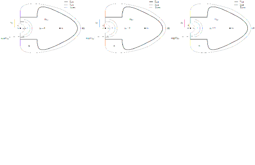
Figure 7: A schematic representation of $\mathsf{D}_{k,\eta}$.

Following the procedure of Section 3.3.1, we can consider the Friedrichs extension $\Delta_{f,h}^{\mathcal{M},(1)}(\mathsf{D}_{k,\eta})$ (which has different boundary conditions from the mixed Laplacian $\Delta_{f,h}^{\textsc{M},(1)}$ introduced in Proposition 33, hence the different notation) of the closed quadratic form

$$Q_{f,h}^{\mathcal{M},(1)}(\mathsf{D}_{k,\eta})(u,w)=\langle\mathsf{d}_{f,h}u,\mathsf{d}_{f,h}w\rangle_{L^{2}(\mathsf{D}_{k,\eta})}+\langle\mathsf{d}^{*}_{f,h}u,\mathsf{d}^{*}_{f,h}w\rangle_{L^{2}(\mathsf{D}_{k,\eta})},$$

for all $u,w\in\mathcal{D}\big{(}Q_{f,h}^{\mathcal{M},(1)}(\mathsf{D}_{k,\eta})\big{)}$, where

$$\mathcal{D}\big{(}Q_{f,h}^{\mathcal{M},(1)}(\mathsf{D}_{k,\eta})\big{)} :=\big{\{}w\in\Lambda^{1}L^{2}(\mathsf{D}_{k,\eta}), \mathsf{d}_{f,h}w\text{ and }\mathsf{d}^{*}_{f,h}w\in\Lambda L^{2}(\mathsf{D}_{k,\eta})\text{ with }$$

$$\quad\quad\mathbf{n}w|_{\Sigma_{k,\mathbf{N}}}=0,\mathbf{t}w|_{\Sigma_{k,\mathbf{D}}}=0,\text{ and }w|_{\Sigma_{k,\mathbf{FD}}}=0\big{\}}.$$

Let $w\in\mathcal{D}\big{(}Q_{f,h}^{\mathcal{M},(1)}(\mathsf{D}_{k,\eta})\big{)}$ and $\varphi$ be a real-valued Lipschitz function on $\overline{\mathsf{D}_{k,\eta}}$. Since $w|_{\Sigma_{k,\mathbf{FD}}}=0$ and $\nabla f\cdot\mathsf{n}_{\mathsf{\Omega}_{k}^{\textsc{M}}}=0$ on $\Gamma_{k,\mathbf{D}}^{\text{M}}\supset\Sigma_{k,\mathbf{D}}$, one has using the same arguments as those used to prove Lemma 34,

$$Q_{f,h}^{\mathcal{M},(1)}(\mathsf{D}_{k,\eta})(w,e^{\frac{2}{h}\varphi}w) =h^{2}\big{\|}\mathsf{d}(e^{\frac{\varphi}{h}}w)\big{\|}^{2}_{L^{2}(\mathsf{D}_{k,\eta})}+h^{2}\big{\|}\mathsf{d}^{*}(e^{\frac{\varphi}{h}}w)\big{\|}^{2}_{L^{2}(\mathsf{D}_{k,\eta})}$$

$$\quad+\big{\langle}(|\nabla f|^{2}-|\nabla\varphi|^{2}+h\mathcal{L}_{\nabla f}+h\mathcal{L}_{\nabla f}^{*})e^{\frac{\varphi}{h}}w,e^{\frac{\varphi}{h}}w\big{\rangle}_{L^{2}(\mathsf{D}_{k,\eta})}$$

$$\quad+h\int_{\Sigma_{k,\mathbf{N}}}\langle w,w\rangle_{T_{\sigma}^{*}\mathsf{D}_{k,\eta}}\;e^{\frac{2}{h}\varphi}\partial_{\mathsf{n}_{\mathsf{\Omega}_{k}^{\textsc{M}}}}f\,d\sigma$$

$$\geq h^{2}\big{\|}\mathsf{d}(e^{\frac{\varphi}{h}}w)\big{\|}^{2}_{L^{2}(\mathsf{D}_{k,\eta})}+h^{2}\big{\|}\mathsf{d}^{*}(e^{\frac{\varphi}{h}}w)\big{\|}^{2}_{L^{2}(\mathsf{D}_{k,\eta})}$$

$$\quad+\big{\langle}(|\nabla f|^{2}-|\nabla\varphi|^{2}+h\mathcal{L}_{\nabla f}+h\mathcal{L}_{\nabla f}^{*})e^{\frac{\varphi}{h}}w,e^{\frac{\varphi}{h}}w\big{\rangle}_{L^{2}(\mathsf{D}_{k,\eta})},$$ (216)

where we have used that $\partial_{\mathsf{n}_{\mathsf{\Omega}_{k}^{\textsc{M}}}}f\geq 0$ a.e. on $\Gamma_{k,\mathbf{N}}^{\textsc{M}}=\Sigma_{k,\mathbf{N}}$. Thus, using (216) and the same analysis as the one made to prove item $(iii)$ in Proposition 35, there exists $c>0$ such that for $h$ small enough:

$$\sigma\big{(}\Delta_{f,h}^{\mathcal{M},(1)}(\mathsf{D}_{k,\eta})\big{)}\geq ch.$$ (217)

Step 2: Resolvent estimates. When $\mathsf{D}$ is a subdomain of $\Omega$, and $w\in\Lambda^{1}L^{2}(\mathsf{D})$ is such that $\mathsf{d}w$ and $\mathsf{d}^{*}w$ belong to $\Lambda L^{2}(\mathsf{D})$, we define

$$\|w\|_{\mathrm{W}^{1}(\mathsf{D})}^{2}:=\|w\|_{L^{2}(\mathsf{D})}^{2}+\|\mathsf{d}w\|_{L^{2}(\mathsf{D})}^{2}+\|\mathsf{d}^{*}w\|_{L^{2}(\mathsf{D})}^{2}.$$ (218)

Notice that by (215) (with $\varphi=0$), it holds

$$\|\mathsf{u}^{(1)}_{k}\|_{\mathrm{W}^{1}(\mathsf{\Omega}_{k}^{\textsc{M}})}\leq Ch^{-1/2}.$$ (219)

By (217) and since $\lambda(\mathsf{\Omega}_{k}^{\textsc{M}})$ is exponentially small as $h$ goes to $0$ (see (183)), the distance of $\lambda(\mathsf{\Omega}_{k}^{\textsc{M}})$ to $\sigma\big{(}\Delta_{f,h}^{\mathcal{M},(1)}(\mathsf{D}_{k,\eta})\big{)}$ is bounded from below by $ch/2$, as $h\to 0$. Then, adopting the notation of [28, p. 56], and using (213) and (216), we obtain using resolvent estimates as in the proof of [28, Proposition 6.5] (with, in our context, $K(h)=\{\lambda(\mathsf{\Omega}_{k}^{\textsc{M}})\}$),

$$\big{(}\Delta_{f,h}^{\mathcal{M},(1)}(\mathsf{D}_{k,\eta})-\lambda(\mathsf{\Omega}_{k}^{\textsc{M}})\big{)}^{-1}(x,y)=\widehat{O}(e^{-\frac{1}{h}\mathsf{d}_{a}(x,y)}\big{)}\text{ for all }x,y\in\mathsf{D}_{k,\eta}.$$ (220)

The $\widehat{O}$ in (220) means that for any $x,y\in\mathsf{D}_{k,\eta}$ and $\epsilon>0$, there exist neighborhoods $V_{x}$ and $V_{y}$ in $\mathsf{D}_{k,\eta}$ of $x$ and $y$ respectively such that for $h$ small enough,

$$\big{\|}\big{(}\Delta_{f,h}^{\mathcal{M},(1)}(\mathsf{D}_{k,\eta})-\lambda(\mathsf{\Omega}_{k}^{\textsc{M}})\big{)}^{-1}w\|_{\mathrm{W}^{1}(V_{x})}\leq e^{-\frac{1}{h}(\mathsf{d}_{a}(x,y)-\epsilon)}\|w\|_{L^{2}(V_{y})},$$

for all $w\in\Lambda^{1}L^{2}(\mathsf{D}_{k,\eta})$ supported in $V_{y}$. We are now in position to prove Proposition 38.

Step 3: Proof of the Agmon estimate. Let $\chi_{\eta}$ be a smooth cut-off function supported in $\mathsf{B}_{a}(z_{k},2\eta)$ which equals $1$ on $\mathsf{B}_{a}(z_{k},3\eta/2)$ and such that $\nabla\chi_{\eta}\cdot\mathsf{n}_{\mathsf{\Omega}_{k}^{\textsc{M}}}=0$. We claim that

$$\text{$(1-\chi_{\eta})\mathsf{u}^{(1)}_{k}\in\mathcal{D}(\Delta_{f,h}^{\mathcal{M},(1)}(\mathsf{D}_{k,\eta}))$ and $\Delta_{f,h}^{\mathcal{M},(1)}(\mathsf{D}_{k,\eta})((1-\chi_{\eta})\mathsf{u}^{(1)}_{k})=\Delta_{f,h}^{(1)}((1-\chi_{\eta})\mathsf{u}^{(1)}_{k})$}.$$ (221)

To prove (221), we use the integration by parts formula [26, Equation (120)] on $\mathsf{D}_{k,\eta}$ with, using the notation there, $u=(1-\chi_{\eta})\mathsf{u}^{(1)}_{k}$ and an arbitrary $v\in\mathcal{D}\big{(}Q_{f,h}^{\mathcal{M},(1)}(\mathsf{D}_{k,\eta})\big{)}$ and we observe that all the boundary terms vanish. To do so, we check that $u=(1-\chi_{\eta})\mathsf{u}^{(1)}_{k}$ satisfies the required regularity, and that the boundary terms are zero. This shows that $Q_{f,h}^{\mathcal{M},(1)}(\mathsf{D}_{k,\eta})(u,v)=\langle\Delta_{f,h}^{(1)}(u),v\rangle_{L^{2}(\mathsf{D}_{k,\eta})}$ is bounded by $C(u)\|v\|_{L^{2}(\mathsf{D}_{k,\eta})}$. Thus $u\in\mathcal{D}(\Delta_{f,h}^{\mathcal{M},(1)}(\mathsf{D}_{k,\eta}))$, and $\Delta_{f,h}^{\mathcal{M},(1)}(\mathsf{D}_{k,\eta})u=\Delta_{f,h}^{(1)}u$.

Let us give some more details on the regularity and trace of $u=(1-\chi_{\eta})\mathsf{u}^{(1)}_{k}$. It is easy to check that $u\in\mathcal{D}\big{(}Q_{f,h}^{\mathcal{M},(1)}(\mathsf{D}_{k,\eta})\big{)}$. Moreover, $\mathbf{n}\mathsf{d}_{f,h}u=0$ on $\Sigma_{k,\mathbf{N}}$ and $\mathsf{d}^{*}_{f,h}u=0$ on $\Sigma_{k,\mathbf{FD}}\cup\Sigma_{k,\mathbf{D}}$ are consequences of the fact that $\mathsf{u}^{(1)}_{k}\in\mathcal{D}(\Delta_{f,h}^{\text{M},(1)}(\mathsf{\Omega}_{k}^{\textsc{M}}))$ and $u=0$ in a neighborhood of $\overline{\Sigma_{k,\mathbf{FD}}}$ in $\overline{\mathsf{D}_{k,\eta}}$. In particular, $\mathsf{d}^{*}_{f,h}u=0\text{ on }\Sigma_{k,\mathbf{D}}$, since, $\mathsf{d}_{f,h}^{*}u=-\nabla\chi_{\eta}\cdot\mathsf{u}^{(1)}_{k}=0$ on $\Sigma_{k,\mathbf{D}}$ (because $\mathsf{d}_{f,h}^{*}\mathsf{u}^{(1)}_{k}=0$ and $\mathbf{t}\mathsf{u}^{(1)}_{k}=0$ on $\Gamma_{k,\mathbf{D}}^{\text{M}}\supset\Sigma_{k,\mathbf{D}}$). This yields $Q_{f,h}^{\mathcal{M},(1)}(\mathsf{D}_{k,\eta})(u,v)=\langle\Delta_{f,h}^{(1)}u,v\rangle_{L^{2}(\mathsf{D}_{k,\eta})}$, using [26, Equation (120)], since $v\in\mathcal{D}\big{(}Q_{f,h}^{\mathcal{M},(1)}(\mathsf{D}_{k,\eta})\big{)}$, $\mathbf{n}\mathsf{d}_{f,h}u=0$ on $\Sigma_{k,\mathbf{N}}$ and $\mathsf{d}^{*}_{f,h}u=0$ on $\Sigma_{k,\mathbf{FD}}\cup\Sigma_{k,\mathbf{D}}$, and thus concludes the proof of 221.

We have, using (221), and since $\mathsf{D}_{k,\eta}\subset\mathsf{\Omega}_{k}^{\textsc{M}}$,

$$\big{(}\Delta_{f,h}^{\text{M},(1)}(\mathsf{D}_{k,\eta})-\lambda(\mathsf{\Omega}_{k}^{\textsc{M}})\big{)}((1-\chi_{\eta})\mathsf{u}^{(1)}_{k})=\big{[}\Delta_{f,h}^{(1)},(1-\chi_{\eta})\big{]}\mathsf{u}^{(1)}_{k}$$

is supported in $\overline{\mathsf{B}_{a}(z_{k},2\eta)}\setminus\mathsf{B}_{a}(z_{k},3\eta/2)$ (we used here the commutator brackets notation). Using (219) and (220), and the fact that $\big{[}\Delta_{f,h}^{(1)},(1-\chi_{\eta})\big{]}$ is a bounded linear operator from $\Lambda^{1}\mathrm{W}^{1}(\mathsf{D}_{k,\eta})$ to $\Lambda^{1}L^{2}(\mathsf{D}_{k,\eta})$, for all $x\in\mathsf{D}_{k,\eta}$ and $\epsilon>0$, there exists a neighborhood $V_{x}$ of $x$ in $\mathsf{D}_{k,\eta}$ such that for $h$ small enough:

$$\|(1-\chi_{\eta})\mathsf{u}^{(1)}_{k}\|_{\mathrm{W}^{1}(V_{x})}\leq e^{\frac{\epsilon}{h}}e^{-\frac{1}{h}(\mathsf{d}_{a}(x,z_{k})-2\eta)}\,\|\mathsf{u}^{(1)}_{k}\|_{\mathrm{W}^{1}(\mathsf{D}_{k,\eta})}\leq e^{\frac{\epsilon}{h}}e^{-\frac{1}{h}(\mathsf{d}_{a}(x,z_{k})-3\eta)}.$$

Proposition 38 is a consequence of the previous estimate, a compactness argument, and the fact that $\mathsf{u}^{(1)}_{k}=\chi_{\eta}\mathsf{u}^{(1)}_{k}+(1-\chi_{\eta})\mathsf{u}^{(1)}_{k}$ and $\|e^{\frac{1}{h}\mathsf{d}_{a}(x,z_{k})}\chi_{\eta}\mathsf{u}^{(1)}_{k}\|_{\mathrm{W}^{1}(\mathsf{\Omega}_{k}^{\textsc{M}})}\leq e^{\frac{3\eta}{h}}$ (by (219) and the continuity of the Agmon distance $\mathsf{d}_{a}(\cdot,z_{k})$).    

Quasi-modes associated with $(z_{k})_{k=1,\ldots,n}$

The principal eigenform $\mathsf{u}^{(1)}_{k}$ of $\Delta_{f,h}^{\textsc{M},(1)}(\mathsf{\Omega}_{k}^{\textsc{M}})$ introduced in Proposition 36 (see (209)) will be used as a quasi-mode for $\Delta_{f,h}^{\mathsf{Di},(1)}(\Omega)$. To do so, we multiply it by a smooth cut-off function $\chi_{k}^{\textsc{M}}$ whose gradient is supported as close as needed to $\Gamma_{k,\mathbf{N}}^{\textsc{M}}$ and so that $\chi_{k}^{\textsc{M}}\mathsf{u}^{(1)}_{k}$ belongs to the form domain of $\Delta_{f,h}^{\mathsf{Di},(1)}(\Omega)$, namely $\Lambda^{1}H^{1}_{\mathbf{T}}(\Omega)$ (as required by item 1 in Proposition 26, see also (119)). More precisely, we have the following result.

Proposition 39.

Let us assume that the assumptions of Proposition 38 hold. Let $\mathsf{u}^{(1)}_{k}$ be defined by (209). Let $\beta>0$ and $\chi_{k}^{\textsc{M}}(\beta):\overline{\mathsf{\Omega}_{k}^{\textsc{M}}}\to[0,1]$ be a $\mathcal{C}^{\infty}$ function such that

$$\chi_{k}^{\textsc{M}}(\beta)=1\text{ on }\big{\{}x\in\overline{\mathsf{\Omega}_{k}^{\textsc{M}}},\ \mathsf{d}_{\overline{\Omega}}(x,\overline{\Gamma_{k,\mathbf{N}}^{\textsc{M}}})>2\beta\big{\}},$$ (222)

and,

$$\chi_{k}^{\textsc{M}}(\beta)=0\text{ on }\big{\{}x\in\overline{\mathsf{\Omega}_{k}^{\textsc{M}}},\ \mathsf{d}_{\overline{\Omega}}(x,\overline{\Gamma_{k,\mathbf{N}}^{\textsc{M}}})\leq\beta\big{\}},$$ (223)

where we recall that $\mathsf{d}_{\,\overline{\Omega}}$ denotes the geodesic distance in $\overline{\Omega}$. We extend $\chi_{k}^{\textsc{M}}(\beta)$ by $0$ on $\overline{\Omega}\setminus\overline{\mathsf{\Omega}_{k}^{\textsc{M}}}$, and thus $\chi_{k}^{\textsc{M}}(\beta)\in\mathcal{C}^{\infty}(\overline{\Omega})$ (see Figure 8 for a schematic representation of the support of $\chi_{k}^{\textsc{M}}$). Then, one defines

$$\mathsf{v}_{k}^{(1)}:=\frac{\chi_{k}^{\textsc{M}}(\beta)\mathsf{u}_{k}^{(1)}}{\|\chi_{k}^{\textsc{M}}(\beta)\mathsf{u}_{k}^{(1)}\|_{L^{2}(\Omega)}},$$ (224)

for any $\beta\in(0,\beta_{0})$ with $\beta_{0}>0$ small enough so that $\chi_{k}^{\textsc{M}}(\beta)\neq 0$. For ease of notation, we do not refer to $\beta$ when writing $\mathsf{v}_{k}^{(1)}$. Then

$$\mathsf{v}_{k}^{(1)}\in\Lambda^{1}H^{1}_{\mathbf{T}}(\Omega)\cap\Lambda^{1}\mathcal{C}^{\infty}_{c}(\overline{\Omega}).$$

Finally, for any $\delta>0$, there exists $h_{\delta}>0$ such that for all $h\in(0,h_{\delta})$ and $\beta\in(0,\beta_{0})$:

$$\big{\|}\mathsf{d}_{f,h}\mathsf{v}_{k}^{(1)}\big{\|}^{2}_{L^{2}(\Omega)}+\big{\|}\mathsf{d}^{*}_{f,h}\mathsf{v}_{k}^{(1)}\big{\|}^{2}_{L^{2}(\Omega)}\leq C\lambda(\mathsf{\Omega}_{k}^{\textsc{M}})+e^{\frac{\delta}{h}}e^{-\frac{2}{h}\inf_{{\rm supp}\nabla\chi_{k}^{\textsc{M}}(\beta)}\mathsf{d}_{a}(\cdot,z_{k})},$$

where $C>0$ is independent of $h$, $\beta$, and $\delta$.

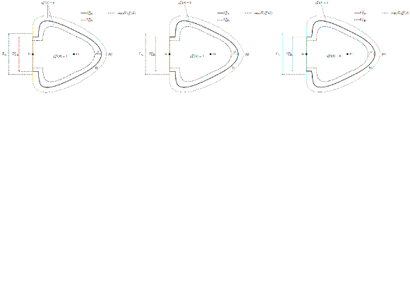
Figure 8: Schematic representation of the cut-off function $\chi_{k}^{\textsc{M}}(\beta)$, see Proposition 39. The support of $\nabla\chi_{k}^{\textsc{M}}(\beta)$ is as close as needed to $\overline{\Gamma_{k,\mathbf{N}}^{\textsc{M}}}$, and $\overline{\Gamma_{k,\mathbf{N}}^{\textsc{M}}}$ can be as closed as needed to $\partial\Omega\setminus\Gamma_{z_{k}}$.

Notice that since $\overline{\Sigma_{z_{k}}}$ is included in the open subset $\Gamma_{k,\mathbf{D}}^{\textsc{M}}$ of $\partial\mathsf{\Omega}_{k}^{\textsc{M}}=\Gamma_{k,\mathbf{D}}^{\textsc{M}}\cup\overline{\Gamma_{k,\mathbf{N}}^{\textsc{M}}}$ (see item 1 in Proposition 30), from (222), for $\beta>0$ small enough,

$$\chi_{k}^{\textsc{M}}(\beta)=1\text{ in a neighborhood of }\overline{\Sigma_{z_{k}}}\text{ in }\overline{\mathsf{\Omega}_{k}^{\textsc{M}}},$$ (225)

or equivalently, in a neighborhood of $\overline{\Sigma_{z_{k}}}$ in $\overline{\Omega}$, by (180)-(135)). In addition, one also has that, since $x_{0}\in{\mathsf{\Omega}_{k}^{\textsc{M}}}$, for $\beta>0$ small enough,

$$\chi_{k}^{\textsc{M}}(\beta)=1\text{ in a neighborhood of }x_{0}\text{ in }{\mathsf{\Omega}_{k}^{\textsc{M}}}\text{ (or equivalently, in $\Omega$).}$$ (226)

In the following, we assume that $\beta>0$ is small enough such that (225) and (226) hold.

Proof.

From (178), $\mathsf{u}_{k}^{(1)},\mathsf{d}\mathsf{u}_{k}^{(1)},\mathsf{d}^{*}\mathsf{u}_{k}^{(1)}\in\Lambda^{1}L^{2}(\mathsf{\Omega}^{\textsc{M}}_{k})$ and $\mathbf{t}\mathsf{u}_{k}^{(1)}|_{\Gamma^{\textsc{M}}_{k,\mathbf{D}}}=0$. Since $\chi_{k}^{\textsc{M}}(\beta)=0$ on $\overline{\Omega}\setminus\overline{\mathsf{\Omega}_{k}^{\textsc{M}}}$,

$$\text{$\mathsf{v}_{k}^{(1)},\mathsf{d}\mathsf{v}_{k}^{(1)},\mathsf{d}^{*}\mathsf{v}_{k}^{(1)}\in\Lambda^{1}L^{2}(\Omega)$}.$$

Since $\chi_{k}^{\textsc{M}}(\beta)=0$ on $\partial{\Omega}\setminus\partial{\mathsf{\Omega}_{k}^{\textsc{M}}}$ and $\mathbf{t}\mathsf{u}_{k}^{(1)}|_{\text{int }(\partial{\Omega}\cap\partial{\mathsf{\Omega}_{k}^{\textsc{M}}})}=0$ (because $\text{int }(\partial\mathsf{\Omega}_{k}^{\textsc{M}}\cap\partial\Omega)={\Gamma_{k,\mathbf{D}}^{\textsc{M}}}$, see item 1 in Proposition 30), it holds: $\mathbf{t}\mathsf{v}_{k}^{(1)}=0$ on $\partial\Omega$. Then, by [26, Lemma 73],

$$\mathsf{v}_{k}^{(1)}\in\Lambda^{1}H^{1}_{\mathbf{T}}(\Omega).$$

In addition, since $\Delta^{(1)}_{f,h}\mathsf{u}_{k}^{(1)}=\lambda(\mathsf{\Omega}_{k}^{\textsc{M}})\mathsf{u}_{k}^{(1)}\in\Lambda^{1}L^{2}(\mathsf{\Omega}_{k}^{\textsc{M}})$ with, on the smooth open subset $\Gamma_{k,\mathbf{D}}^{\textsc{M}}$ of $\mathsf{\Omega}_{k}^{\textsc{M}}$, $\mathbf{t}\mathsf{u}_{k}^{(1)}=0$ and $\mathbf{t}\mathsf{d}_{f,h}^{*}\mathsf{u}_{k}^{(1)}=0$, it holds, by elliptic regularity, $\mathsf{u}_{k}^{(1)}\in\Lambda^{1}\mathcal{C}^{\infty}(\mathsf{\Omega}_{k}^{\textsc{M}}\cup\Gamma_{k,\mathbf{D}}^{\textsc{M}})$. Therefore,

$$\mathsf{v}_{k}^{(1)}\in\Lambda^{1}\mathcal{C}^{\infty}_{c}(\overline{\Omega}).$$

Let us now compute the energy of $\mathsf{v}_{k}^{(1)}$ in $\Omega$. Let us first deal with $\|\chi_{k}^{\textsc{M}}(\beta)\mathsf{u}_{k}^{(1)}\|_{L^{2}(\Omega)}$. First of all, $\|\chi_{k}^{\textsc{M}}(\beta)\mathsf{u}_{k}^{(1)}\|_{L^{2}(\Omega)}=\|\chi_{k}^{\textsc{M}}(\beta)\mathsf{u}_{k}^{(1)}\|_{L^{2}(\mathsf{\Omega}^{\textsc{M}}_{k})}\leq 1$ (we have used that $\|\mathsf{u}_{k}^{(1)}\|_{L^{2}(\Omega)}=1$, $\chi_{k}^{\textsc{M}}(\beta)=0$ on $\overline{\Omega}\setminus\overline{\mathsf{\Omega}_{k}^{\textsc{M}}}$, and $\chi_{k}^{\textsc{M}}\in[0,1]$). On the other hand, It holds,

$$\|\chi_{k}^{\textsc{M}}(\beta)\mathsf{u}_{k}^{(1)}\|_{L^{2}(\mathsf{\Omega}_{k}^{\textsc{M}})}\geq 1-\big{\|}[1-\chi_{k}^{\textsc{M}}(\beta)]\mathsf{u}_{k}^{(1)}\big{\|}_{L^{2}(\mathsf{\Omega}_{k}^{\textsc{M}})}$$

and

$$\big{\|}[1-\chi_{k}^{\textsc{M}}(\beta)]\mathsf{u}_{k}^{(1)}\big{\|}_{L^{2}(\mathsf{\Omega}_{k}^{\textsc{M}})}=\big{\|}[1-\chi_{k}^{\textsc{M}}(\beta)]e^{-\frac{\Psi_{k}}{h}}\,\mathsf{u}_{k}^{(1)}e^{\frac{\Psi_{k}}{h}}\big{\|}_{L^{2}(\mathsf{\Omega}_{k}^{\textsc{M}})},$$

where we introduced the function $\Psi_{k}(x)=\mathsf{d}_{a}(x,z_{k})$. Furthermore, $\chi_{k}^{\textsc{M}}(\beta)=1$ in a neighborhood of $z_{k}$ in $\overline{\Omega}$ (by (225) together with the fact that $z_{k}\in\Sigma_{z_{k}}$). Thus, there exits $c>0$ such that

$$\inf_{\text{supp}(1-\chi_{k}^{\textsc{M}}(\beta))}\Psi_{k}>c.$$

Then, using Proposition 38, one deduces that $\big{\|}[1-\chi_{k}^{\textsc{M}}(\beta)]\mathsf{u}_{k}^{(1)}\big{\|}_{L^{2}(\mathsf{\Omega}_{k}^{\textsc{M}})}=O(e^{-\frac{c}{h}})$, for some $c>0$ and as $h\to 0$. Consequently,

$$\|\chi_{k}^{\textsc{M}}(\beta)\mathsf{u}_{k}^{(1)}\|_{L^{2}(\Omega)}=1+O(e^{-\frac{c}{h}}).$$ (227)

In addition one has, using again Proposition 38,

$$\big{\|}\mathsf{d}_{f,h}(\chi_{k}^{\textsc{M}}(\beta)\mathsf{u}_{k}^{(1)})\big{\|}_{L^{2}(\Omega)} \leq\|\chi_{k}^{\textsc{M}}(\beta)\mathsf{d}_{f,h}\mathsf{u}_{k}^{(1)}\big{\|}_{L^{2}(\mathsf{\Omega}_{k}^{\textsc{M}})}+h\big{\|}\nabla\chi_{k}^{\textsc{M}}(\beta)\wedge\mathsf{u}_{k}^{(1)}\big{\|}_{L^{2}(\mathsf{\Omega}_{k}^{\textsc{M}})}$$

$$\leq\sqrt{\lambda(\mathsf{\Omega}_{k}^{\textsc{M}})}+e^{\frac{\delta}{h}}e^{-\frac{1}{h}\inf_{{\rm supp}\nabla\chi_{k}^{\textsc{M}}(\beta)}\Psi_{k}}.$$

The same inequality holds for $\big{\|}\mathsf{d}^{*}_{f,h}(\chi_{k}^{\textsc{M}}(\beta)\mathsf{u}_{k}^{(1)})\big{\|}_{L^{2}(\Omega)}$ because

$$\big{\|}\mathsf{d}^{*}_{f,h}(\chi_{k}^{\textsc{M}}(\beta)\mathsf{u}_{k}^{(1)})\big{\|}_{L^{2}(\Omega)}\leq\|\chi_{k}^{\textsc{M}}(\beta)\mathsf{d}^{*}_{f,h}\mathsf{u}_{k}^{(1)}\big{\|}_{L^{2}(\mathsf{\Omega}_{k}^{\textsc{M}})}+h\big{\|}\nabla\chi_{k}^{\textsc{M}}(\beta)\cdot\mathsf{u}_{k}^{(1)}\big{\|}_{L^{2}(\mathsf{\Omega}_{k}^{\textsc{M}})}.$$

The proof of Proposition 39 is complete using (227) and (224).    

According to (126), (222), and (223), for any $\gamma>0$, one can choose $\mathsf{\Omega}_{k}^{\textsc{M}}$ in Proposition 30 and $\beta>0$ small enough in Proposition 39 (see Figure 8) such that:

$$\sup_{x\in{\rm supp}\nabla\chi_{k}^{\textsc{M}}(\beta)}\mathsf{d}_{\,\overline{\Omega}}(x,\partial\Omega\setminus\Gamma_{z_{k}})\leq\gamma.$$

Hence, for any $\delta>0$, one can choose $\beta>0$ and $\mathsf{\Omega}_{k}^{\textsc{M}}$ such that:

$$\inf_{{\rm supp}\nabla\chi_{k}^{\textsc{M}}(\beta)}\mathsf{d}_{a}(\cdot,z_{k})\geq\inf_{\partial\Omega\setminus\Gamma_{z_{k}}}\mathsf{d}_{a}(\cdot,z_{k})-\delta/4$$ (228)

Then, once (228) is satisfied, one can use (183) and Proposition 39 with such $\beta>0$ and $\mathsf{\Omega}_{k}^{\textsc{M}}$ fixed as a function $\delta$, to obtain the following result.

Corollary 40.

Let us assume that the assumptions of Proposition 38 hold. For any $\delta>0$, there exists a domain $\mathsf{\Omega}_{k}^{\textsc{M}}$, $\beta>0$, and $h_{\delta}>0$ such that for $h\in(0,h_{\delta})$:

$$\big{\|}\mathsf{d}_{f,h}\mathsf{v}_{k}^{(1)}\big{\|}^{2}_{L^{2}(\Omega)}+\big{\|}\mathsf{d}^{*}_{f,h}\mathsf{v}_{k}^{(1)}\big{\|}^{2}_{L^{2}(\Omega)}\leq Che^{-\frac{2}{h}(f(z_{k})-f(x_{0}))}+e^{\frac{\delta}{h}}e^{-\frac{2}{h}\inf_{\partial\Omega\setminus\Gamma_{z_{k}}}\mathsf{d}_{a}(\cdot,z_{k})},$$

where $C>0$ is independent of $h>0$ and $\delta>0$.

By Corollary 40, and because $\inf_{z\in\partial\Omega\setminus\Gamma_{z_{k}}}\mathsf{d}_{a}(z,z_{k})>0$ and $f(z_{k})>f(x_{0})$, there exists $c>0$ such that for $h$ small enough:

$$\big{\|}\mathsf{d}_{f,h}\mathsf{v}_{k}^{(1)}\big{\|}^{2}_{L^{2}(\Omega)}+\big{\|}\mathsf{d}^{*}_{f,h}\mathsf{v}_{k}^{(1)}\big{\|}^{2}_{L^{2}(\Omega)}\leq Ce^{-\frac{c}{h}}.$$

This implies that $\mathsf{v}_{k}^{(1)}$ is a quasi-mode associated with the spectrum in $[0,ch]$ of $\Delta_{f,h}^{\textsc{M},(1)}(\mathsf{\Omega}_{k}^{\textsc{M}})$ because, using in addition Lemma 11 and the fact that, by Proposition 39, $\mathsf{v}_{k}^{(1)}\in\Lambda^{1}H^{1}_{\mathbf{T}}(\Omega)=\mathcal{D}(Q_{f,h}^{\mathsf{Di},(1)}(\Omega))$, it holds:

$$\big{\|}\big{[}1-\pi_{[0,\mathsf{c}h]}(\Delta_{f,h}^{\mathsf{Di},(1)}(\Omega))\big{]}\mathsf{v}_{k}^{(1)}\big{\|}^{2}_{L^{2}(\Omega)}\leq Ce^{-\frac{c}{h}}.$$ (229)

Proofs of the main results

In this section, we give the proofs of the main results stated in Section 1.2.4.

Proofs of Theorem 1, Proposition 7, Theorem 2, and Corollary 8

The quasi-modes for $\mathsf{L}^{\mathsf{Di},(0)}_{f,h}(\Omega)$ and $\mathsf{L}^{\mathsf{Di},(1)}_{f,h}(\Omega)$ are defined as follows.

Definition 41.

Let us assume that ($\Omega$-$f$) is satisfied. Then, one defines for $k\in\{1,\ldots,n\}$ (see (209) and (224)):

$$\mathsf{f}_{k}^{(1)}:=e^{\frac{1}{h}f}\mathsf{v}_{k}^{(1)}\in\Lambda^{1}H^{1}_{w,\mathbf{T}}(\Omega).$$

For $r\in(0,\min_{\partial\Omega}f-f(x_{0}))$, consider $\chi_{r}\in\mathcal{C}^{\infty}_{c}(\Omega)$ such that $\chi_{r}=1$ on $\{f<\min_{\partial\Omega}f-r\}$. Then, one defines:

$$\mathsf{u}^{(0)}:=\frac{\chi_{r}}{\|\chi_{r}\|_{L^{2}_{w}(\Omega)}}\in\mathcal{C}^{\infty}_{c}(\Omega).$$

For ease of notation, we do not refer to $r>0$ in the notation of $\mathsf{u}^{(0)}$. Recall that the family $\{\mathsf{f}_{1}^{(1)},\ldots,\mathsf{f}_{n}^{(1)}\}$ depends on the parameter $\delta>0$ introduced in Corollary 40. Let us now check that there exist $r>0$ and $\delta>0$ such that the family of quasi-modes $\{\mathsf{f}_{1}^{(1)},\ldots,\mathsf{f}_{n}^{(1)}\}\cup\{\mathsf{u}^{(0)}\}$ introduced in Definition 41 satisfies the assumptions of Propositions 26 and 27. As explained at the end of this section, Theorem 1, Proposition 7, Theorem 2, and Corollary 8 are then consequences of the results of Propositions 26 and 27.

Let us start with the following lemma.

Lemma 42.

Let us assume that ($\Omega$-$f$) is satisfied. Let $\{\mathsf{f}_{1}^{(1)},\ldots,\mathsf{f}_{n}^{(1)}\}$ and $\mathsf{u}^{(0)}$ be as introduced in Definition 41. Then, item 1 in Proposition 26 is satisfied as well as item 2(b). Furthermore, there exists $C>0$ such that for all $h$ small enough:

$$\big{\|}u_{h}-\mathsf{u}^{(0)}\big{\|}_{L_{w}^{2}(\Omega)}\leq C\,h^{-\frac{d}{4}+\frac{1}{2}}e^{-\frac{1}{h}(f(z_{1})-f(x_{0})-r)}.$$ (230)

Finally, (28) is satisfied.

Proof.

Item 1 in Proposition 26 is satisfied by Definition 41. First of all, because $\{x_{0}\}=\operatorname*{arg\,min}_{\overline{\Omega}}f$ (see Lemma 4) and since $\chi_{r}=1$ near $x_{0}$ in $\Omega$ (see Definition 41), it holds, using Laplace’s method, in the limit $h\to 0$:

$$\|\chi_{r}\|_{L^{2}_{w}(\Omega)}^{2}=\kappa_{x_{0}}h^{\frac{d}{2}}e^{-\frac{2}{h}f(x_{0})}\big{(}1+O(h)\big{)},$$ (231)

where $\kappa_{x_{0}}$ is defined in (186). Recall that from Corollary 25 (see also (122) for the definition of $\pi_{h}^{(0)}$), the $L^{2}_{w}(\Omega)$-orthogonal projector $\pi_{h}^{(0)}$ associated with $\mathsf{L}_{f,h}^{\mathsf{Di},(0)}(\Omega)$ has rank $1$. Because $\mathsf{u}^{(0)}\in\mathcal{D}(Q_{f,h}^{\mathsf{Di},(0)}(\Omega))$ (see Proposition 24 and Section 1.2.3), it holds thanks to Lemma 11:

$$\big{\|}(1-\pi_{h}^{(0)})\mathsf{u}^{(0)}\big{\|}_{L^{2}_{w}(\Omega)}^{2}\leq\frac{1}{\mathsf{c}}Q_{f,h}^{\mathsf{Di},(0)}(\Omega)(\mathsf{u}^{(0)})=\frac{h}{2\mathsf{c}}\|\nabla\mathsf{u}^{(0)}\|_{L^{2}_{w}(\Omega)}^{2}.$$

Using (231) and because $\chi_{r}\in\mathcal{C}^{\infty}_{c}(\Omega)$ such that $\chi_{r}=1$ on $\{f<\min_{\partial\Omega}f-r\}$, one has for $h$ small enough:

$$\frac{h}{2}\|\nabla\mathsf{u}^{(0)}\|_{L^{2}_{w}(\Omega)}^{2}=\frac{h}{2}\frac{\|\nabla\chi_{r}\|_{L^{2}_{w}(\Omega)}^{2}}{\|\chi_{r}\|_{L^{2}_{w}(\Omega)}^{2}}\leq C\|\nabla\chi_{r}\|_{L^{\infty}(\Omega)}^{2}\,h^{-\frac{d}{2}+1}\,e^{-\frac{2}{h}(\min_{\partial\Omega}f-f(x_{0})-r)}.$$

Hence, because $f(z_{1})=\min_{\partial\Omega}f$ (see Lemma 4 and (15)), $\mathsf{u}^{(0)}$ satisfies item 2(b) in Proposition 26. In addition, one has:

$$\big{\|}(1-\pi_{h}^{(0)})\mathsf{u}^{(0)}\big{\|}_{L^{2}_{w}(\Omega)}^{2}\leq C\|\nabla\chi_{r}\|_{L^{\infty}(\Omega)}^{2}\,h^{-\frac{d}{2}+1}\,e^{-\frac{2}{h}(f(z_{1})-f(x_{0})-r)}.$$

Choosing $r>0$ small enough, it hence holds for $h$ small enough:

$$\|\pi_{h}^{(0)}\mathsf{u}^{(0)}\|_{L^{2}_{w}(\Omega)}=1+O(e^{-\frac{c}{h}})\neq 0,$$

and then (using in addition the fact that $u_{h}>0$, $\mathsf{u}^{(0)}\geq 0$ on $\Omega$, and $\mathsf{u}^{(0)}\neq 0$),

$$u_{h}=\frac{\pi_{h}^{(0)}\mathsf{u}^{(0)}}{\|\pi_{h}^{(0)}\mathsf{u}^{(0)}\|_{L^{2}_{w}(\Omega)}}=\frac{\mathsf{u}^{(0)}}{\|\pi_{h}^{(0)}\mathsf{u}^{(0)}\|_{L^{2}_{w}(\Omega)}}+\frac{(\pi_{h}^{(0)}-1)\mathsf{u}^{(0)}}{\|\pi_{h}^{(0)}\mathsf{u}^{(0)}\|_{L^{2}_{w}(\Omega)}}\text{ in }L^{2}_{w}(\Omega).$$

Equation (230) is a direct consequence of the three last equations. Moreover, the latter equation implies

$$\int_{\Omega}u_{h}\,e^{-\frac{2}{h}f}=(1+O(e^{-\frac{c}{h}}))\Big{[}\int_{\Omega}\mathsf{u}^{(0)}\,e^{-\frac{2}{h}f}+e_{h}\Big{]},$$

where

$$|e_{h}|\leq\big{\|}(1-\pi_{h}^{(0)})\mathsf{u}^{(0)}\big{\|}_{L^{2}_{w}(\Omega)}\big{\|}1\big{\|}_{L^{2}_{w}(\Omega)}\leq Ce^{-\frac{1}{h}(f(x_{0})+c_{r})},$$

where $c_{r}=f(z_{1})-f(x_{0})-r>0$ (since $r\in(0,f(z_{1})-f(x_{0}))$). On the other hand, from (231) together with the fact that $\int_{\Omega}\chi\,e^{-\frac{2}{h}f}$ has the same asymptotic equivalent as $\int_{\Omega}\chi^{2}\,e^{-\frac{2}{h}f}$ when $h\to 0$,

$$\int_{\Omega}\mathsf{u}^{(0)}\,e^{-\frac{2}{h}f}=h^{d/4}\sqrt{\kappa_{x_{0}}}e^{-\frac{1}{h}f(x_{0})}\big{(}1+O(h)\big{)}.$$

This proves (28) and concludes the proof of Lemma 42.    

Let us now check that $\{\mathsf{f}_{1}^{(1)},\ldots,\mathsf{f}_{n}^{(1)}\}$ satisfies item 2(a) and item 3 in Proposition 26.

Lemma 43.

Assume that ($\Omega$-$f$) is satisfied. Let $\{\mathsf{f}_{1}^{(1)},\ldots,\mathsf{f}_{n}^{(1)}\}$ be the family of $1$-forms introduced in Definition 41. Let $k\in\{1,\ldots,n\}$. Then, for any $\delta>0$, there exists $h_{\delta}>0$ such that for $h\in(0,h_{\delta})$:

$$\big{\|}\big{(}1-\pi_{h}^{(1)}\big{)}\mathsf{f}_{k}^{(1)}\big{\|}_{H^{1}_{w}(\Omega)}^{2}\leq Ch^{-2}e^{-\frac{2}{h}(f(z_{k})-f(x_{0}))}+e^{\frac{\delta}{h}}e^{-\frac{2}{h}(\inf_{\partial\Omega\setminus\Gamma_{z_{k}}}\mathsf{d}_{a}(\cdot,z_{k}))},$$ (232)

and for all $\ell\in\{1,\ldots,n\}$, $\ell\neq k$,

$$\big{|}\big{\langle}\mathsf{f}_{k}^{(1)},\mathsf{f}_{\ell}^{(1)}\big{\rangle}_{L^{2}_{w}(\Omega)}\big{|}\leq e^{\frac{\delta}{h}}e^{-\frac{1}{h}\mathsf{d}_{a}(z_{k},z_{\ell})}.$$ (233)

In particular, choosing $\delta>0$ small enough, $\{\mathsf{f}_{1}^{(1)},\ldots,\mathsf{f}_{n}^{(1)}\}$ satisfies items 2(a) and 3 in Proposition 26, and if (25) and (26) hold, then $\{\mathsf{f}_{1}^{(1)},\ldots,\mathsf{f}_{n}^{(1)}\}$ satisfies items 1 and 2 in Proposition 27.

Proof.

Using Lemma 11 and Proposition 10,

$$\big{\|}\big{[}1-\pi_{[0,\mathsf{c}h]}(\Delta_{f,h}^{\mathsf{Di},(1)}(\Omega))\big{]}\mathsf{v}_{k}^{(1)}\big{\|}^{2}_{L^{2}(\Omega)}\leq\frac{\big{\|}\mathsf{d}_{f,h}\mathsf{v}_{k}^{(1)}\big{\|}^{2}_{L^{2}(\Omega)}+\big{\|}\mathsf{d}^{*}_{f,h}\mathsf{v}_{k}^{(1)}\big{\|}^{2}_{L^{2}(\Omega)}}{\mathsf{c}h}.$$

Therefore, using Corollary 40, for any $\delta>0$, there exists $h_{\delta}>0$ such that for $h\in(0,h_{\delta})$:

$$\big{\|}\big{[}1-\pi_{[0,\mathsf{c}h]}(\Delta_{f,h}^{\mathsf{Di},(1)}(\Omega))\big{]}\mathsf{v}_{k}^{(1)}\big{\|}^{2}_{L^{2}(\Omega)}\leq Ce^{-\frac{2}{h}(f(z_{k})-f(x_{0}))}+e^{\frac{\delta}{h}}e^{-\frac{2}{h}(\inf_{\partial\Omega\setminus\Gamma_{z_{k}}}\mathsf{d}_{a}(\cdot,z_{k}))}.$$

Let us prove that this inequality also holds in $\Lambda^{1}H^{1}(\Omega)$. Set $\mathsf{v}_{k,\pi}^{(1)}=\big{[}1-\pi_{[0,\mathsf{c}h]}(\Delta_{f,h}^{\mathsf{Di},(1)}(\Omega))\big{]}\mathsf{v}_{k}^{(1)}$. It holds using Proposition 10,

$$\big{[}1-\pi_{[0,\mathsf{c}h]}(\Delta_{f,h}^{\mathsf{Di},(2)}(\Omega))\big{]}\mathsf{d}_{f,h}\mathsf{v}_{k}^{(1)}=\mathsf{d}_{f,h}\mathsf{v}_{k,\pi}^{(1)}=h\mathsf{d}\mathsf{v}_{k,\pi}^{(1)}+\nabla f\wedge\mathsf{v}_{k,\pi}^{(1)}.$$

Therefore,

$$h\|\mathsf{d}\mathsf{v}_{k,\pi}^{(1)}\|_{L^{2}(\Omega)}\leq\|\mathsf{d}_{f,h}\mathsf{v}_{k}^{(1)}\|_{L^{2}(\Omega)}+C\|\mathsf{v}_{k,\pi}^{(1)}\|_{L^{2}(\Omega)}.$$

Similarly, one has $h\|\mathsf{d}^{*}\mathsf{v}_{k,\pi}^{(1)}\|_{L^{2}(\Omega)}\leq\|\mathsf{d}^{*}_{f,h}\mathsf{v}_{k}^{(1)}\|_{L^{2}(\Omega)}+C\|\mathsf{v}_{k,\pi}^{(1)}\|_{L^{2}(\Omega)}$. Hence, using also the standard Gaffney inequality in $\Omega$ (see [79]), since $\mathsf{v}_{k,\pi}^{(1)}\in\Lambda^{1}H^{1}_{\mathbf{T}}(\Omega)$ (by Proposition 39), it holds:

$$C_{\text{Gaffney}}\big{\|}\mathsf{v}_{k,\pi}^{(1)}\big{\|}^{2}_{H^{1}(\Omega)} \leq\big{\|}\mathsf{v}_{k,\pi}^{(1)}\big{\|}^{2}_{L^{2}(\Omega)}+\big{\|}\mathsf{d}\mathsf{v}_{k,\pi}^{(1)}\big{\|}^{2}_{L^{2}(\Omega)}+\big{\|}\mathsf{d}^{*}\mathsf{v}_{k,\pi}^{(1)}\big{\|}^{2}_{L^{2}(\Omega)}$$

$$\leq Ch^{-2}\big{(}\|\mathsf{d}_{f,h}\mathsf{v}_{k}^{(1)}\|_{L^{2}(\Omega)}^{2}+\|\mathsf{d}^{*}_{f,h}\mathsf{v}_{k}^{(1)}\|_{L^{2}(\Omega)}^{2}+\|\mathsf{v}_{k,\pi}^{(1)}\|_{L^{2}(\Omega)}^{2}\big{)}.$$ (234)

This implies that for $h\in(0,h_{\delta})$:

$$\big{\|}\mathsf{v}_{k,\pi}^{(1)}\big{\|}^{2}_{H^{1}(\Omega)}\leq Ch^{-2}\big{[}e^{-\frac{2}{h}(f(z_{k})-f(x_{0}))}+e^{\frac{\delta}{h}}e^{-\frac{2}{h}(\inf_{\partial\Omega\setminus\Gamma_{z_{k}}}\mathsf{d}_{a}(\cdot,z_{k}))}\big{]}.$$ (235)

From (119), it holds:

$$\pi_{[0,\mathsf{c}h]}(\Delta_{f,h}^{\mathsf{Di},(1)}(\Omega))=e^{-\frac{1}{h}f}\pi_{h}^{(1)}e^{\frac{1}{h}f}.$$

Therefore, by definition of $\mathsf{f}_{k}^{(1)}$ (see Definition 41) and from (235),

$$\big{\|}(1-\pi_{h}^{(1)})\mathsf{f}_{k}^{(1)}\big{\|}^{2}_{H^{1}_{w}(\Omega)}\leq Ch^{-2}e^{-\frac{2}{h}(f(z_{k})-f(x_{0}))}+e^{\frac{\delta}{h}}e^{-\frac{2}{h}(\inf_{\partial\Omega\setminus\Gamma_{z_{k}}}\mathsf{d}_{a}(\cdot,z_{k}))}.$$

This proves Equation (232).

Let us now prove (233). One has (see Definition 41) using the triangular inequality for $\mathsf{d}_{a}$,

$$|\big{\langle}\mathsf{f}_{k}^{(1)},\mathsf{f}_{\ell}^{(1)}\big{\rangle}_{L^{2}_{w}(\Omega)}|=|\big{\langle}\mathsf{v}_{k}^{(1)},\mathsf{v}_{\ell}^{(1)}\big{\rangle}_{L^{2}(\Omega)}|\leq e^{-\frac{1}{h}\mathsf{d}_{a}(z_{\ell},z_{k})}\|\mathsf{v}_{k}^{(1)}e^{\frac{1}{h}\mathsf{d}_{a}(\cdot,z_{k})}\|_{L^{2}(\Omega)}\,\|\mathsf{v}_{\ell}^{(1)}e^{\frac{1}{h}\mathsf{d}_{a}(\cdot,z_{\ell})}\|_{L^{2}(\Omega)}.$$

Equation (233) is thus a consequence of the previous inequality together with Proposition 38 and (227) (see also (224)).

Since $f(z_{k})-f(x_{0})>0$, $\mathsf{d}_{a}(z_{k},z_{\ell})>0$, and $\inf_{z\in\partial\Omega\setminus\Gamma_{z_{k}}}\mathsf{d}_{a}(z_{k},z)>0$ (because $\mathsf{d}_{a}$ is a distance), $\{\mathsf{f}_{1}^{(1)},\ldots,\mathsf{f}_{n}^{(1)}\}$ satisfies items 2(a) and 3 in Proposition 26 hold choosing $\delta>0$ small enough in (232) and (233). Finally, since $z_{\ell}\in\partial\Omega\setminus\Gamma_{z_{k}}$ (because $z_{\ell}\notin\mathsf{W}_{+}^{z_{k}}$ and $\Gamma_{z_{k}}\subset\mathsf{W}_{+}^{z_{k}}$, see (14))

$$\mathsf{d}_{a}(z_{k},z_{\ell})\geq\inf_{z\in\partial\Omega\setminus\Gamma_{z_{k}}}\mathsf{d}_{a}(z_{k},z).$$

In addition, $f(z_{k})-f(x_{0})\geq f(z_{1})-f(x_{0})$ and if $k>\ell$, $f(z_{k})-f(z_{1})\geq f(z_{k})-f(z_{\ell})$. Thus, if (25) and (26) hold, then $\{\mathsf{f}_{1}^{(1)},\ldots,\mathsf{f}_{n}^{(1)}\}$ satisfies items 1 and 2 in Proposition 27.    

Lemma 44.

Let us assume that ($\Omega$-$f$) is satisfied. Let $\{\mathsf{f}_{1}^{(1)},\ldots,\mathsf{f}_{n}^{(1)}\}$ be the family of $1$-forms introduced in Definition 41. Let $k,\ell\in\{1,\ldots,n\}^{2}$. Then, it holds,

$$\int_{\Sigma_{z_{\ell}}}\mathsf{f}_{k}^{(1)}\cdot\mathsf{n}_{\Omega}\ e^{-\frac{2}{h}f}d\sigma=\begin{cases}0&\text{ if }k\neq\ell,\\ -\mathsf{b}_{k}\ h^{\mathsf{m}}\ e^{-\frac{1}{h}f(z_{k})}\ (1+O(\sqrt{h}))&\text{ if }k=\ell,\end{cases}$$

where $\mathsf{b}_{k}$ and $\mathsf{m}$ are defined in (186). Let $\mathsf{u}^{(0)}$ be as introduced in Definition 41. Then, for all $k\in\{1,\ldots,n\}$, there exists $c>0$ such that as $h\to 0$:

$$\big{\langle}\nabla\mathsf{u}^{(0)},\mathsf{f}_{k}^{(1)}\big{\rangle}_{L^{2}_{w}(\Omega)}=\begin{cases}\mathsf{K}_{k}h^{\mathsf{p}}\,e^{-\frac{1}{h}(f(z_{1})-f(x_{0}))}(1+O(\sqrt{h}))&\text{ if }k\in\{1,\ldots,n_{0}\},\\ O(e^{-\frac{1}{h}(f(z_{1})-f(x_{0})+c)})&\text{ if }k>n_{0},\end{cases}$$

where $\mathsf{K}_{k}$ and $\mathsf{p}$ are defined in (237) below. In particular, $\{\mathsf{f}_{1}^{(1)},\ldots,\mathsf{f}_{n}^{(1)}\}$ and $\mathsf{u}^{(0)}$ satisfy item 4 in Proposition 26. If moreover (25) and (26) hold, one has as $h\to 0$,

$$\big{\langle}\nabla\mathsf{u}^{(0)},\mathsf{f}_{k}^{(1)}\big{\rangle}_{L^{2}_{w}(\Omega)}=\mathsf{K}_{k}h^{\mathsf{p}}\,e^{-\frac{1}{h}(f(z_{k})-f(x_{0}))}(1+O(\sqrt{h})).$$

Hence, if (25) and (26) hold, $\{\mathsf{f}_{1}^{(1)},\ldots,\mathsf{f}_{n}^{(1)}\}$ and $\mathsf{u}^{(0)}$ satisfy items 3 and 4 in Proposition 27.

Proof.

Recall the definitions of $\mathsf{u}^{(0)}$ and $\{\mathsf{f}_{1}^{(1)},\ldots,\mathsf{f}_{n}^{(1)}\}$ in Definition 41. The proof is divided into several steps.

Step 1. Let us first compute $\int_{\Sigma_{z_{k}}}\mathsf{u}_{k}^{(1)}\cdot\mathsf{n}_{\Omega}\ e^{-\frac{1}{h}f}$. One has since $\overline{\Sigma_{z_{k}}}\subset\Gamma_{k,\mathbf{D}}^{\textsc{M}}$ (see item 1 in Proposition 30),

$$\int_{\Sigma_{z_{k}}}\mathsf{u}_{k}^{(1)}\cdot\mathsf{n}_{\Omega}\ e^{-\frac{1}{h}f}=\int_{\Gamma_{k,\mathbf{D}}^{\textsc{M}}}\mathsf{u}_{k}^{(1)}\cdot\mathsf{n}_{\Omega}\ e^{-\frac{1}{h}f}d\sigma-\int_{\Gamma_{k,\mathbf{D}}^{\textsc{M}}\setminus\Sigma_{z_{k}}}\mathsf{u}_{k}^{(1)}\cdot\mathsf{n}_{\Omega}\ e^{-\frac{1}{h}f}.$$

It holds, using the trace estimate (175) and Proposition 38, for any $\delta>0$, there exists $h_{\delta}>0$ such that for $h\in(0,h_{\delta})$:

$$\Big{|}\int_{\Gamma_{k,\mathbf{D}}^{\textsc{M}}\setminus\Sigma_{z_{k}}}\mathsf{u}_{k}^{(1)}\cdot\mathsf{n}_{\Omega}\ e^{-\frac{1}{h}f}\Big{|}\leq e^{-\frac{1}{h}\inf_{\Gamma_{k,\mathbf{D}}^{\textsc{M}}\setminus\Sigma_{z_{k}}}(\mathsf{d}_{a}(\cdot,z_{k})+f(z_{k}))}e^{\frac{\delta}{h}}.$$

Notice that we have used that $f\geq f(z_{k})$ on $\Gamma_{k,\mathbf{D}}^{\textsc{M}}$ (because $\Gamma_{k,\mathbf{D}}^{\textsc{M}}\subset\Gamma_{z_{k}}\subset\mathsf{W}_{+}^{z_{k}}$, see Lemma 14). Thus, since $\inf_{\Gamma_{k,\mathbf{D}}^{\textsc{M}}\setminus\Sigma_{z_{k}}}\mathsf{d}_{a}(\cdot,z_{k})>0$, for $\delta>0$ small enough, one has for $h$ small enough

$$\Big{|}\int_{\Gamma_{k,\mathbf{D}}^{\textsc{M}}\setminus\Sigma_{z_{k}}}\mathsf{u}_{k}^{(1)}\cdot\mathsf{n}_{\Omega}\ e^{-\frac{1}{h}f}\Big{|}\leq e^{-\frac{1}{h}(f(z_{k})+c)}.$$ (236)

Using (185), it then holds as $h\to 0$:

$$\int_{\Sigma_{z_{k}}}\mathsf{u}^{(1)}_{k}\cdot\mathsf{n}_{\mathsf{\Omega}_{k}^{\textsc{M}}}\ e^{-\frac{1}{h}f}=-\mathsf{b}_{k}h^{\mathsf{m}}\,e^{-\frac{1}{h}f(z_{k})}(1+O(\sqrt{h})),\$$

where $\mathsf{b}_{k}$ and $\mathsf{m}$ are defined in (186).

Step 2. Let us deal with the terms $\int_{\Sigma_{z_{\ell}}}\mathsf{f}_{k}^{(1)}\cdot\mathsf{n}_{\Omega}\,e^{-\frac{1}{h}f}$. One has that $\chi_{k}^{\textsc{M}}(\beta)=0\text{ on }\partial\Omega\setminus\overline{\Gamma_{k,\mathbf{D}}^{\textsc{M}}}.$ Indeed, $\chi_{k}^{\textsc{M}}(\beta)$ is supported in $\overline{\mathsf{\Omega}_{k}^{\textsc{M}}}$ (see (222), and (223)) and $\overline{\mathsf{\Omega}_{k}^{\textsc{M}}}\cap\partial\Omega=\partial\mathsf{\Omega}_{k}^{\textsc{M}}\cap\partial\Omega=\overline{\Gamma_{k,\mathbf{D}}^{\textsc{M}}}$ (see item 1 Proposition 30). In particular, because $\overline{\Gamma_{k,\mathbf{D}}^{\textsc{M}}}\subset\Gamma_{z_{k}}$, and $\Gamma_{z_{k}}\cap\Sigma_{\ell}\subset\Gamma_{z_{k}}\cap\Gamma_{z_{\ell}}=\emptyset$ when $k\neq\ell$ (see the line after the proof of Lemma 4 and (16)), $\chi_{k}^{\textsc{M}}(\beta)=0$ on $\Sigma_{z_{\ell}}$ when $k\neq\ell$. Then, one has using (224), (225) and (227),

$$\int_{\Sigma_{z_{\ell}}}\mathsf{f}_{k}^{(1)}\cdot\mathsf{n}_{\Omega}\ e^{-\frac{2}{h}f} =\int_{\Sigma_{z_{\ell}}}\mathsf{v}_{k}^{(1)}\cdot\mathsf{n}_{\Omega}\ e^{-\frac{1}{h}f}d\sigma$$

$$=\frac{1}{\|\chi_{k}^{\textsc{M}}(\beta)\mathsf{u}_{k}^{(1)}\|_{L^{2}(\Omega)}}\int_{\Sigma_{z_{\ell}}}\chi_{k}^{\textsc{M}}(\beta)\mathsf{u}_{k}^{(1)}\cdot\mathsf{n}_{\Omega}\ e^{-\frac{1}{h}f}$$

$$=(1+O(e^{-\frac{c}{h}}))\times\begin{cases}0&\text{ if }k\neq\ell,\\ \int_{\Sigma_{z_{k}}}\mathsf{u}_{k}^{(1)}\cdot\mathsf{n}_{\Omega}\ e^{-\frac{1}{h}f}&\text{ if }k=\ell,\end{cases}$$

$$=\begin{cases}0&\text{ if }k\neq\ell,\\ -\mathsf{b}_{k}\ h^{\mathsf{m}}\ e^{-\frac{1}{h}f(z_{k})}\ (1+O(\sqrt{h}))&\text{ if }k=\ell.\end{cases}$$

This proves the first statement in Lemma 44. In particular, $\{\mathsf{f}_{1}^{(1)},\ldots,\mathsf{f}_{n}^{(1)}\}$ satisfies item 4(b) in Proposition 26 and item 4 in Proposition 27.

Step 3. Let us finally deal with the terms $\big{\langle}\nabla\mathsf{u}^{(0)},\mathsf{f}_{k}^{(1)}\big{\rangle}_{L^{2}_{w}(\Omega)}$. One has, since $\chi_{r}=0$ on $\partial\Omega$, from (224),

$$\big{\langle}\nabla\mathsf{u}^{(0)},\mathsf{f}_{k}^{(1)}\big{\rangle}_{L^{2}_{w}(\Omega)} =\frac{1}{\|\chi_{r}\|_{L^{2}_{w}(\Omega)}}\big{\langle}\nabla\chi_{r},e^{-\frac{1}{h}f}\mathsf{v}_{k}^{(1)}\big{\rangle}_{L^{2}(\Omega)}$$

$$=-\frac{1}{\|\chi_{r}\|_{L^{2}_{w}(\Omega)}}\big{\langle}\nabla(1-\chi_{r}),e^{-\frac{1}{h}f}\mathsf{v}_{k}^{(1)}\big{\rangle}_{L^{2}(\Omega)}$$

$$=\frac{1}{\|\chi_{r}\|_{L^{2}_{w}(\Omega)}}\Big{[}h^{-1}\big{\langle}(1-\chi_{r}),e^{-\frac{1}{h}f}\mathsf{d}^{*}_{f,h}\mathsf{v}_{k}^{(1)}\big{\rangle}_{L^{2}(\Omega)}-\int_{\partial\Omega}e^{-\frac{1}{h}f}\mathsf{v}_{k}^{(1)}\cdot\mathsf{n}_{\Omega}\Big{]}$$

$$=\frac{1}{\|\chi_{r}\|_{L^{2}_{w}(\Omega)}}\Big{[}h^{-1}\big{\langle}(1-\chi_{r})e^{-\frac{1}{h}f},\mathsf{d}^{*}_{f,h}\mathsf{v}_{k}^{(1)}\big{\rangle}_{L^{2}(\Omega)}-\int_{\partial\Omega\cap{\rm supp}\chi_{k}^{\textsc{M}}(\beta)}e^{-\frac{1}{h}f}\mathsf{v}_{k}^{(1)}\cdot\mathsf{n}_{\Omega}\Big{]}.$$

Let us first deal with the boundary term in the previous equality. Because $\chi_{k}^{\textsc{M}}(\beta)=0$ on $\partial\Omega\setminus\overline{\Gamma_{k,\mathbf{D}}^{\textsc{M}}}$, from (224) and (227), it holds:

$$\int_{\partial\Omega\cap{\rm supp}\chi_{k}^{\textsc{M}}(\beta)}e^{-\frac{1}{h}f}\mathsf{v}_{k}^{(1)}\cdot\mathsf{n}_{\Omega} =(1+O(e^{-\frac{c}{h}}))\int_{\Gamma_{k,\mathbf{D}}^{\textsc{M}}}\chi_{k}^{\textsc{M}}(\beta)e^{-\frac{1}{h}f}\mathsf{u}_{k}^{(1)}\cdot\mathsf{n}_{\Omega}$$

$$=(1+O(e^{-\frac{c}{h}}))\Big{[}\int_{\Gamma_{k,\mathbf{D}}^{\textsc{M}}}(\chi_{k}^{\textsc{M}}(\beta)-1)e^{-\frac{1}{h}f}\mathsf{u}_{k}^{(1)}\cdot\mathsf{n}_{\Omega}+\int_{\Gamma_{k,\mathbf{D}}^{\textsc{M}}}e^{-\frac{1}{h}f}\mathsf{u}_{k}^{(1)}\cdot\mathsf{n}_{\Omega}\Big{]}.$$

It holds, from (225),

$$\Big{|}\int_{\Gamma_{k,\mathbf{D}}^{\textsc{M}}}(\chi_{k}^{\textsc{M}}(\beta)-1)e^{-\frac{1}{h}f}\mathsf{u}_{k}^{(1)}\cdot\mathsf{n}_{\Omega}\Big{|}=\Big{|}\int_{\Gamma_{k,\mathbf{D}}^{\textsc{M}}\setminus\Sigma_{z_{k}}}(\chi_{k}^{\textsc{M}}(\beta)-1)e^{-\frac{1}{h}f}\mathsf{u}_{k}^{(1)}\cdot\mathsf{n}_{\Omega}\Big{|}\leq C\Big{|}\int_{\Gamma_{k,\mathbf{D}}^{\textsc{M}}\setminus\Sigma_{z_{k}}}e^{-\frac{1}{h}f}\mathsf{u}_{k}^{(1)}\cdot\mathsf{n}_{\Omega}\Big{|}.$$

Thus from (236) and (185), it then holds as $h\to 0$:

$$\int_{\partial\Omega\cap{\rm supp}\chi_{k}^{\textsc{M}}(\beta)}e^{-\frac{1}{h}f}\mathsf{v}_{k}^{(1)}\cdot\mathsf{n}_{\Omega}=-\mathsf{b}_{k}h^{\mathsf{m}}\,e^{-\frac{1}{h}f(z_{k})}(1+O(\sqrt{h})).$$

Hence, as $h\to 0$, one has using (231) (see also (186)):

$$-\frac{1}{\|\chi_{r}\|_{L^{2}_{w}(\Omega)}}\int_{\partial\Omega\cap{\rm supp}\chi_{k}^{\textsc{M}}(\beta)}e^{-\frac{1}{h}f}\mathsf{v}_{k}^{(1)}\cdot\mathsf{n}_{\Omega}=\mathsf{K}_{k}h^{\mathsf{p}}\,e^{-\frac{1}{h}(f(z_{k})-f(x_{0}))}(1+O(\sqrt{h})),\$$

with

$$\mathsf{K}_{k}=\frac{\mathsf{b}_{k}}{\sqrt{\kappa_{x_{0}}}}=\sqrt{\mathsf{A}_{x_{0},z_{k}}}\ \text{and}\ \mathsf{p}=\mathsf{m}-\frac{d}{4}=-\frac{1}{2},\text{ where $\mathsf{A}_{x_{0},z_{k}}$ is defined in \eqref{eq.ax0zk}.}$$ (237)

Let us now deal with the error term $\big{\langle}(1-\chi_{r})e^{-\frac{1}{h}f},\mathsf{d}^{*}_{f,h}\mathsf{v}_{k}^{(1)}\big{\rangle}_{L^{2}(\Omega)}$. Using Proposition 39 and Corollary 40, for any $\delta>0$, there exists $h_{\delta}>0$ such that for $h\in(0,h_{\delta})$:

$$\big{|}\big{\langle}(1-\chi_{r}),e^{-\frac{1}{h}f}\mathsf{d}^{*}_{f,h}\mathsf{v}_{k}^{(1)}\big{\rangle}_{L^{2}(\Omega)}\big{|} \leq Ce^{-\frac{1}{h}\min_{{\rm supp}(1-\chi_{r})}f}\|\mathsf{d}^{*}_{f,h}\mathsf{v}_{k}^{(1)}\|_{L^{2}(\Omega)}$$

$$\leq Ce^{-\frac{1}{h}(f(z_{1})-r)}\big{[}e^{-\frac{1}{h}(f(z_{k})-f(x_{0}))}+e^{\frac{\delta}{h}}e^{-\frac{1}{h}(\inf_{z\in\partial\Omega\setminus\Gamma_{z_{k}}}\mathsf{d}_{a}(z_{k},z))}\big{]}.$$

Therefore, using (231),

$$\frac{\big{|}\big{\langle}(1-\chi_{r})e^{-\frac{1}{h}f},\mathsf{d}^{*}_{f,h}\mathsf{v}_{k}^{(1)}\big{\rangle}_{L^{2}(\Omega)}\big{|}}{\|\chi_{r}\|_{L^{2}_{w}(\Omega)}} \leq C\big{[}h^{-d/4}e^{-\frac{1}{h}(f(z_{k})-f(x_{0}))}e^{-\frac{1}{h}(f(z_{1})-f(x_{0})-r)}$$

$$\qquad+e^{\frac{\delta}{h}}e^{-\frac{1}{h}(\inf_{z\in\partial\Omega\setminus\Gamma_{z_{k}}}\mathsf{d}_{a}(z_{k},z))}e^{-\frac{1}{h}(f(z_{1})-f(x_{0})-r)}\big{]}$$

$$\leq e^{-\frac{1}{h}\mathsf{E}_{k}(r,\delta)},$$

where, for $r>0$ and $\delta>0$ small enough, one can choose $\mathsf{E}_{k}(r,\delta)>f(z_{1})-f(x_{0})$. Moreover, if (25) and (26) hold, then $\inf_{z\in\partial\Omega\setminus\Gamma_{z_{k}}}\mathsf{d}_{a}(z_{k},z)>f(z_{k})-f(z_{1})$ and $f(z_{1})-f(x_{0})>f(z_{k})-f(z_{1})$. Thus, for $r>0$ and $\delta>0$ small enough, one can choose $\mathsf{E}_{k}(r,\delta)>f(z_{k})-f(x_{0})$. The proof of Lemma 44 is complete.    

In this section, we proved (see Lemmata 42, 43, and 44) that the quasi-modes $\{\mathsf{f}_{1}^{(1)},\ldots,\mathsf{f}_{n}^{(1)}\}\cup\{\mathsf{u}^{(0)}\}$ satisfy all the assumptions of Propositions 26 and 27. We can now conclude the proofs of Theorem 1, Proposition 7, Theorem 2, and Corollary 8, using the results of Propositions 26 and 27. Theorem 1 is a consequence of Propositions 26 and 27 together with the formulas (186) and (237) for the constants $\mathsf{b}_{k}$, $\mathsf{m}$, $\mathsf{K}_{k}$, and $\mathsf{p}$. Proposition 7 is a consequence of Lemma 42 and Proposition 26 (notice that using Lemma 4, Proposition 7 is also a consequence of the results of [58]: we thus here provide a new proof using $1$-forms). Theorem 2 is a consequence of Theorem 1 and Proposition 7 together with (21). Corollary 8 is a consequence of Theorem 1, Proposition 7, and (22). It remains to prove Theorem 3.

Generalization to deterministic initial conditions: proof of Theorem 3

The proof of Theorem 3 relies on so-called leveling results (see Corollary 47 below) which only requires that $f:\overline{\Omega}\to\mathbb{R}$ is a $\mathcal{C}^{\infty}$ function which satisfies item 1 in ($\Omega$-$f$). For $F\in\mathcal{C}^{\infty}(\partial\Omega,\mathbb{R})$, let us define

$$\forall x\in\overline{\Omega},\ w_{h}(x)=\mathbb{E}_{x}[F(X_{\tau})],$$ (238)

where $\tau$ is defined by (2).

Leveling result on $w_{h}$

For any closed subset $\mathsf{F}\subset\mathbb{R}^{d}$, one denotes by

$$\tau_{\mathsf{F}}=\inf\{t\geq 0\,|\,X_{t}\in\mathsf{F}\}$$

the first time the process (1) hits $\mathsf{F}$ (in particular, $\tau=\tau_{\Omega^{c}}$). Let $x_{0}$ be a local minimum of $f$ in $\Omega$. Let us recall that ${\mathsf{B}(x_{0},h)}$ is the open ball centred at $x_{0}$ of radius $h$. Let us assume that $h$ is small enough so that $\overline{\mathsf{B}}(x_{0},h)\subset\Omega$, where $\overline{\mathsf{B}}(x_{0},h)$ is the closure of ${\mathsf{B}}(x_{0},h)$. The function

$$\mathsf{p}_{x_{0}}:x\mapsto\mathbb{P}_{x}[\tau_{\Omega^{c}}<\tau_{\overline{\mathsf{B}}(x_{0},h)}]$$

is called the committor function (or the equilibrium potential) between $\Omega^{c}$ and $\overline{\mathsf{B}}(x_{0},h)$. We have the following precise leveling result on $\mathsf{p}_{x_{0}}:\overline{\Omega}\to\mathbb{R}$.

Proposition 45.

Let us assume that $f:\overline{\Omega}\to\mathbb{R}$ is a $\mathcal{C}^{\infty}$ Morse function which satisfies item 1 in ($\Omega$-$f$). Let $\mathsf{K}$ be a compact subset of $\{f<\min_{\partial\Omega}f\}$. Then, there exist $C_{\mathsf{K}}>0$ and $h_{0}>0$ such that for all $h\in(0,h_{0})$ and $x\in\mathsf{K}$:

$$\mathsf{p}_{x_{0}}(x)\leq C_{\mathsf{K}}\,h^{-d}e^{-\frac{2}{h}(\min_{\partial\Omega}f-f(x))}.$$ (239)

We refer to Figure 9 for a schematic representation of $\{f<\min_{\partial\Omega}f\}$ and $\mathsf{B}(x_{0},h)$ (recall that since item 1 in ($\Omega$-$f$) holds, $f$ satisfies item 1 in Lemma 4).

Figure 9: Schematic representation of $\{f<\min_{\partial\Omega}f\}$ and $\mathsf{B}(x_{0},h)$. On the figure $\partial\{f<\min_{\partial\Omega}f\}\cap\partial\Omega=\{z_{1},z_{2}\}$.

Proof.

The proof of this result is inspired by the proofs of [9, Lemma 4.6] and [53, Proposition 7.9]. Let $x\in\Omega$. If $x\in\overline{\mathsf{B}}(x_{0},h)$, then $\mathsf{p}_{x_{0}}=0$. Let us thus deal with the case when $x\in\Omega\setminus\overline{\mathsf{B}}(x_{0},h)$.

Step 1. First inequality for $\mathsf{p}_{x_{0}}(x)$ using capacities.

In this step, we prove Equation (242) below. Let us denote by $\mathsf{d}_{\mathbb{R}^{d}}$ the standard Euclidean distance in $\mathbb{R}^{d}$. Let $G_{h}$ be the Green function of $\mathsf{L}^{\mathsf{Di},(0)}_{f,h}(\Omega\setminus\overline{\mathsf{B}}(x_{0},h))$, see [9, Equation (2.3)]. Set for $x\in\Omega\setminus\overline{\mathsf{B}}(x_{0},h)$,

$$c=\mathsf{d}_{\mathbb{R}^{d}}(x,\Omega^{c}\cup\overline{\mathsf{B}}(x_{0},h))/2.$$ (240)

Define

$$\text{$\rho=ch>0$ and $R=\rho/3$}.$$

On the one hand, using this couple $(\rho,R)$ in the proof of [9, Lemma 4.6], one deduces that there exists $C_{H}>0$ such that for all $x\in\Omega\setminus\overline{\mathsf{B}}(x_{0},h)$, $h\in(0,1]$,

$$\sup_{z\in\partial\mathsf{B}(x,\rho)}G_{h}(x,z)\leq C_{H}^{\pi\rho/R}\inf_{z\in\partial\mathsf{B}(x,\rho)}G_{h}(x,z).$$ (241)

Notice that $c$ depends on $h$ and $x$ (which was a priori not the case in [9, Lemma 4.6]). Let us explain more precisely why (241) remains valid in our setting. To get Equation (241), one uses $k$ times the Harnack inequality [34] (see also [9, Lemma 4.1]) on $k$ balls $\mathsf{B}(x_{i},\rho)$ where $x_{i}\in\partial\mathsf{B}(x,\rho)$ with $\mathsf{B}(x_{i},R)\cap\mathsf{B}(x_{i+1},R)\neq\emptyset$ ($i=1,\ldots,k$, $x_{k+1}=x_{1}$), and where $k\leq\pi\rho/R$. The constant $C_{H}$ in (241) is the one from the Harnack inequality used on each $\mathsf{B}(x_{i},R)$. In addition, this constant $C_{H}$ depends on $h^{-2}R^{2}$ and thus can be chosen independently of $h$ since for all $x\in\Omega\setminus\overline{\mathsf{B}}(x_{0},h)$ and $h>0$,

$$h^{-2}R^{2}\leq\mathsf{d}_{\mathbb{R}^{d}}^{2}(x,\Omega^{c}\cup\{x_{0}\})/6^{2}\leq\mathsf{M}_{0}^{2}/36,$$

where $\mathsf{M}_{0}:=\max_{y\in\overline{\Omega}}\mathsf{d}_{\mathbb{R}^{d}}(y,\Omega^{c}\cup\{x_{0}\})$. The condition $h\leq 1$ in (241) ensures that we can use the Harnack inequality, since for all $x\in\Omega\setminus\overline{\mathsf{B}}(x_{0},h)$ and all $i=1,\ldots,k$,

$${\mathsf{B}(x_{i},2R)}\subset\Omega\setminus\overline{\mathsf{B}}(x_{0},h),$$

which follows from the fact that, if $h\leq 1$, $\rho+2R=5\mathsf{d}_{\mathbb{R}^{d}}(x,\Omega^{c}\cup\overline{\mathsf{B}}(x_{0},h))h/6<\mathsf{d}_{\mathbb{R}^{d}}(x,\Omega^{c}\cup\overline{\mathsf{B}}(x_{0},h))$. Finally notice that we have that

$$C_{H}^{\pi\rho/R}=C_{H}^{\pi/3}.$$

On the other hand, using the arguments of the proof of [53, Proposition 7.9] with $\mathcal{C}=\mathsf{B}(x,\rho)$ there, together with (241), one deduces that there exists $C>0$ such that for all $x\in\Omega\setminus\overline{\mathsf{B}}(x_{0},h)$ and $h$ small enough:

$$\mathsf{p}_{x_{0}}(x)\leq C\frac{\text{cap}(\mathsf{B}(x,\rho),\Omega^{c})}{\text{cap}(\mathsf{B}(x,\rho),\mathsf{B}(x_{0},h)\cup\Omega^{c})},$$ (242)

where we recall that (see [9, Section 2]) for two subsets $\mathsf{C}$ and $\mathsf{D}$ of $\mathbb{R}^{d}$ such that $\overline{\mathsf{C}}\cap\overline{\mathsf{D}}=\emptyset$,

$${\rm cap}({\mathsf{C}},\mathsf{D}) =\frac{h}{2}\inf_{\varphi\in H_{\mathsf{C},\mathsf{D}}}\int_{\mathbb{R}^{d}\setminus(\mathsf{D}\cup\mathsf{C})}\big{|}\nabla\varphi(x)\big{|}^{2}e^{-\frac{2}{h}f(x)}dx,$$ (243)

where

$$H_{\mathsf{C},\mathsf{D}}=\big{\{}\varphi\in H^{1}(\mathbb{R}^{d}),\,\varphi(x)=1\text{ for }x\in\mathsf{C},\,\varphi(x)=0\text{ for }x\in\mathsf{D}\}.$$

Step 2. Upper bound on $\text{cap}(\mathsf{B}(x,\rho),\Omega^{c})$ and lower bound on $\text{cap}(\mathsf{B}(x,\rho),\mathsf{B}(x_{0},h)\cup\Omega^{c})$.

Let us first obtain a lower bound on $\text{cap}(\mathsf{B}(x,\rho),\mathsf{B}(x_{0},h)\cup\Omega^{c})$. By the variational principle for capacities (243), it holds:

$$\text{cap}(\mathsf{B}(x,\rho),\mathsf{B}(x_{0},h)\cup\Omega^{c})\geq\text{cap}(\mathsf{B}(x,\rho),\mathsf{B}(x_{0},h)).$$

Let $\mathsf{K}$ be a compact subset of $\Omega$. Following the proof of [53, Lemma 7.10] (see also [9, Proposition 4.7]) with here $\rho:[0,1]\to\Omega$ a smooth path connecting $x$ to $x_{0}$ and such that $t\in[0,1]\mapsto f(\rho(t))$ is decreasing, there exists $C>0$ such that for all $x\in\mathsf{K}$ and $h>0$ (recall $x_{0}$ is the global minimum of $f$ in $\overline{\Omega}$),

$$\text{cap}(\mathsf{B}(x,\rho),\mathsf{B}(x_{0},h))\geq Ch^{d}e^{-\frac{2}{h}f(x)}.$$ (244)

Let us now deal with $\text{cap}(\mathsf{B}(x,\rho),\Omega^{c})$. Let $\mathsf{U}_{h}$ be the subdomain of $\{f<\min_{\partial\Omega}f\}$ such that $\overline{\mathsf{U}_{h}}\subset\{f<\min_{\partial\Omega}f\}$ and for all $x\in\partial\mathsf{U}_{h}$, $\mathsf{d}_{\mathbb{R}^{d}}(x,{\{f<\min_{\partial\Omega}f\}}^{c})=h$. It then follows that for $h$ small enough,

$$\min_{\{f<\min_{\partial\Omega}f\}\setminus{\mathsf{U}_{h}}}f\geq\min_{\partial\Omega}f-\epsilon h,$$ (245)

for some $\epsilon>0$ independent of $h$. Let $\phi_{h}$ be a smooth function on $\mathbb{R}^{d}$ such that $\phi_{h}=0$ on $\{f<\min_{\partial\Omega}f\}^{c}$, $\phi_{h}=1$ on $\mathsf{U}_{h}$, and for some $C>0$ independent of $h$,

$$\|\nabla\phi_{h}\|_{L^{\infty}(\Omega)}\leq Ch^{-1}.$$ (246)

Assume now that $\mathsf{K}$ is a compact subset of $\{f<\min_{\partial\Omega}f\}$. Then, for $h$ small enough, it holds for all $x\in\mathsf{K}$:

$${\mathsf{B}(x,\rho)}\subset\mathsf{U}_{h},$$

where we recall $\rho=ch>0$ where $c$ is defined by (240) and satisfies $c\leq\mathsf{M}_{0}/2$. Hence, using the variational formula (243), it holds, for $h$ small enough and all $x\in\mathsf{K}$,

$$\text{cap}(\mathsf{B}(x,\rho),\Omega^{c})\leq\frac{h}{2}\int_{\mathbb{R}^{d}}|\nabla\phi_{h}|^{2}e^{-\frac{2}{h}f}=\frac{h}{2}\int_{\{f<\min_{\partial\Omega}f\}\setminus{\mathsf{U}_{h}}}|\nabla\phi_{h}|^{2}e^{-\frac{2}{h}f}.$$

Using in addition (245) and (246), one deduces that for $h$ small enough and all $x\in\mathsf{K}$,

$$\text{cap}(\mathsf{B}(x,\rho),\Omega^{c})\leq Ce^{-\frac{2}{h}(\min_{\partial\Omega}f-ch)}$$ (247)

where $C>0$ is a constant independent of $x\in\mathsf{K}$ and $h$. In conclusion, Equations (242), (244), and (247) imply (239). This concludes the proof of Proposition 45.    

The following result (which is proved as [52, Lemma 1] or [73, Lemma 3]), gives a leveling results on $w_{h}$ in $\mathsf{B}(x_{0},h)$.

Lemma 46.

Let us assume that $f:\overline{\Omega}\to\mathbb{R}$ is a $\mathcal{C}^{\infty}$ Morse function. Let $x_{0}$ be a local minimum of $f$ in $\Omega$. Then, it holds for $h$ small enough

$$\sup_{x\in{\mathsf{B}(x_{0},h)}}|w_{h}(x)-w_{h}(x_{0})|\leq C\sqrt{h}\,w_{h}(x_{0})$$

The two previous results have the following consequence on $w_{h}$.

Corollary 47.

Let us assume that $f:\overline{\Omega}\to\mathbb{R}$ is a $\mathcal{C}^{\infty}$ Morse function which satisfies item 1 in ($\Omega$-$f$). Let $\mathsf{K}$ be a compact subset of $\{f<\min_{\partial\Omega}f\}$. Then, for $h$ small enough and uniformly in $x\in\mathsf{K}$, one has,

$$w_{h}(x)=w_{h}(x_{0})(1+O(\sqrt{h}))+O(h^{-d}e^{-\frac{2}{h}(\min_{\partial\Omega}f-\max_{\mathsf{K}}f)}).$$

Let us mention that a similar result was proved in [26, Section 5.1.4] using [29, Theorem 1] when $f$ has no critical point on the boundary of $\Omega$. When this is no longer the case, [29, Theorem 1] does not apply and we prove this result using the strong Markov property together with Proposition 45 and Lemma 46.

Proof.

Let $\mathsf{K}$ be a compact subset of $\{f<\min_{\partial\Omega}f\}$ and $x\in\mathsf{K}$. Then write:

$$\mathbb{E}_{x}[F(X_{\tau_{\Omega^{c}}})]=\mathbb{E}_{x}\big{[}F(X_{\tau_{\Omega^{c}}})\,\mathbf{1}_{\tau_{\mathsf{B}(x_{0},h)}<\tau_{\Omega^{c}}}\big{]}+\mathbb{E}_{x}\big{[}F(X_{\tau_{\Omega^{c}}})\mathbf{1}_{\tau_{\mathsf{B}(x_{0},h)}\geq\tau_{\Omega^{c}}}\big{]}.$$ (248)

By the strong Markov property,

$$\mathbb{E}_{x}\big{[}F(X_{\tau_{\Omega^{c}}})\mathbf{1}_{\tau_{\mathsf{B}(x_{0},h)}<\tau_{\Omega^{c}}}\big{]}=\mathbb{E}_{x}\big{[}\mathbf{1}_{\tau_{\mathsf{B}(x_{0},h)}<\tau_{\Omega^{c}}}\mathbb{E}_{X_{\tau_{\mathsf{B}(x_{0},h)}}}[F(X_{\tau_{\Omega^{c}}})]\big{]}.$$

Using Proposition 45 and Lemma 46, for all $h$ small enough and $x\in\mathsf{K}$, it holds:

$$\mathbb{E}_{x}\big{[}F(X_{\tau_{\Omega^{c}}})\,\mathbf{1}_{\tau_{\mathsf{B}_{r_{h}}(x_{0})}<\tau_{\Omega^{c}}}\big{]}=\big{(}1+O(e^{-\frac{c}{h}})\big{)}\big{(}1+O(\sqrt{h})\big{)}w_{h}(x_{0}),\text{ uniformly in $x\in\mathsf{K}$},$$ (249)

where $c>0$ is any constant such that $c<2(\min_{\partial\Omega}f-\max_{\mathsf{K}}f)$. Let us now deal with the last term in (248). For $x\in\mathsf{K}$, it holds:

$$\mathbb{E}_{x}\big{[}F(X_{\tau_{\Omega^{c}}})\mathbf{1}_{\tau_{\mathsf{B}(x_{0},h)}\geq\tau_{\Omega^{c}}}\big{]}\leq\|F\|_{L^{\infty}(\partial\Omega)}\mathbb{P}_{x}[\tau_{\mathsf{B}(x_{0},h)}\geq\tau_{\Omega^{c}}].$$

Using Proposition 45, it thus holds for $h$ small enough:

$$\max_{x\in\mathsf{K}}\mathbb{E}_{x}\big{[}F(X_{\tau_{\Omega^{c}}})\mathbf{1}_{\tau_{\mathsf{B}(x_{0},h)}\geq\tau_{\Omega^{c}}}\big{]}\leq Ch^{-d}e^{-\frac{2}{h}(\min_{\partial\Omega}f-\max_{\mathsf{K}}f)}.$$

Together with (249) and (248), this concludes the proof of Corollary 47.    

Proof of Theorem 3

We are now in position to prove Theorem 3.

Proof of Theorem 3.

Let us assume that Assumption ($\Omega$-$f$) is satisfied. Let us define for $\alpha\in\mathbb{R}$,

$$\mathsf{K}_{\alpha}:=\{f\leq\alpha\}.$$

In the following we consider $f(x_{0})<\alpha<\min_{\partial\Omega}f$ so that

$$\mathsf{K}_{\alpha}\text{ is a non empty compact subset of }\{f<\min_{\partial\Omega}f\}.$$

Write

$$\mathbb{E}_{\nu_{h}}[F(X_{\tau_{\Omega}})]={\mathsf{Z}_{h}^{-1}}\int_{\Omega\setminus\mathsf{K}_{\alpha}}w_{h}\,{u}_{h}\,e^{-\frac{2}{h}f}+{\mathsf{Z}_{h}^{-1}}\int_{\mathsf{K}_{\alpha}}w_{h}\,{u}_{h}\,e^{-\frac{2}{h}f},$$ (250)

where we have defined $\mathsf{Z}_{h}:=\int_{\Omega}{u}_{h}\,e^{-\frac{2}{h}f}$. Let us deal with the first term in the right hand side of (250). It holds:

$${\mathsf{Z}_{h}^{-1}}\int_{\Omega\setminus\mathsf{K}_{\alpha}}w_{h}\,{u}_{h}\,e^{-\frac{2}{h}f}\leq\|F\|_{L^{\infty}(\partial\Omega)}\ {\mathsf{Z}_{h}^{-1}}\int_{\Omega\setminus\mathsf{K}_{\alpha}}{u}_{h}\,e^{-\frac{2}{h}f}.$$

Moreover, using Lemma 42, it holds (see Definition 41)

$$\int_{\Omega\setminus\mathsf{K}_{\alpha}}{u}_{h}\,e^{-\frac{2}{h}f}=\frac{\int_{\Omega\setminus\mathsf{K}_{\alpha}}\chi_{r}e^{-\frac{2}{h}f}}{\|\chi_{r}\|_{L^{2}_{w}}}+O\big{(}h^{-\frac{d}{4}+\frac{1}{2}}e^{-\frac{1}{h}(f(z_{1})-f(x_{0})-r)}\big{)}\sqrt{\int_{\Omega\setminus\mathsf{K}_{\alpha}}e^{-\frac{2}{h}f}}.$$

Recall that when $h\to 0$ (see Proposition 7, (231), and (186)),

$$\mathsf{Z}_{h}=\sqrt{\kappa_{0}}\,h^{d/4}\,e^{-\frac{1}{h}f(x_{0})}(1+O(h))\ \text{and}\ \|\chi_{r}\|_{L^{2}_{w}}=\sqrt{\kappa_{0}}\,h^{d/4}\,e^{-\frac{1}{h}f(x_{0})}(1+O(h)).$$

Then, since $f\geq\alpha$ on $\Omega\setminus\mathsf{K}_{\alpha}$, there exists $\beta>0$ such that:

$${\mathsf{Z}_{h}^{-1}}\int_{\Omega\setminus\mathsf{K}_{\alpha}}{u}_{h}\,e^{-\frac{2}{h}f}\leq Ch^{-\beta}\big{[}e^{-\frac{2}{h}(\alpha-f(x_{0}))}+e^{-\frac{1}{h}(f(z_{1})+\alpha-2f(x_{0})-r)}\big{]}.$$

Therefore, because $\min_{\partial\Omega}f=f(z_{1})\geq\alpha$, for any $r>0$, it holds for $h$ small enough:

$${\mathsf{Z}_{h}^{-1}}\int_{\Omega\setminus\mathsf{K}_{\alpha}}{u}_{h}\,e^{-\frac{2}{h}f}\leq e^{-\frac{2}{h}(\alpha-f(x_{0})-r)}.$$ (251)

In conclusion, the first term in the right hand side of (250) satisfies the following upper bound: for any $r>0$, it holds for $h$ small enough:

$${\mathsf{Z}_{h}^{-1}}\int_{\Omega\setminus\mathsf{K}_{\alpha}}w_{h}\,{u}_{h}\,e^{-\frac{2}{h}f}\leq e^{-\frac{2}{h}(\alpha-f(x_{0})-r)}.$$ (252)

Let us now deal with the second term in the right hand side of (250). Using Corollary 47 with $\mathsf{K}=\mathsf{K}_{\alpha}$ there, it holds:

$${\mathsf{Z}_{h}^{-1}}\int_{\mathsf{K}_{\alpha}}w_{h}\,{u}_{h}\,e^{-\frac{2}{h}f}=\Big{[}w_{h}(x_{0})(1+O(\sqrt{h}))+O(h^{-d}e^{-\frac{2}{h}(\min_{\partial\Omega}f-\max_{\mathsf{K}_{\alpha}}f)})\Big{]}\times\frac{\int_{\mathsf{K}_{\alpha}}{u}_{h}\,e^{-\frac{2}{h}f}}{\int_{\Omega}{u}_{h}\,e^{-\frac{2}{h}f}}.$$

In addition, by (251),

$$\frac{\int_{\mathsf{K}_{\alpha}}{u}_{h}\,e^{-\frac{2}{h}f}}{\int_{\Omega}{u}_{h}\,e^{-\frac{2}{h}f}}=1-{\mathsf{Z}_{h}^{-1}}\int_{\Omega\setminus\mathsf{K}_{\alpha}}{u}_{h}\,e^{-\frac{2}{h}f}=1+O(e^{-\frac{c}{h}}).$$

Thus, the second term in the right hand side of (250) satisfies the equivalent in the limit $h\to 0$:

$${\mathsf{Z}_{h}^{-1}}\int_{\mathsf{K}_{\alpha}}w_{h}\,{u}_{h}\,e^{-\frac{2}{h}f}=\Big{[}w_{h}(x_{0})(1+O(\sqrt{h}))+O(h^{-d}e^{-\frac{2}{h}(\min_{\partial\Omega}f-\alpha)})\Big{]}(1+O(e^{-\frac{c}{h}})).$$ (253)

Choosing $r>0$ small enough, Equations (35) and (36) when $x=x_{0}$ are then consequences of (252), (253), (250) together with (30) and (31) in Theorem 2, and the fact that $f(x_{0})<\alpha<\min_{\partial\Omega}f$. To obtain (35) and (36) uniformly on all $x$ in any compact subset $\mathsf{K}$ of $\{f<\min_{\partial\Omega}f\}$, one uses in addition Corollary 47 with $\mathsf{K}_{\alpha}$ where $\mathsf{K}$ is such that $\mathsf{K}\subset\mathsf{K}_{\alpha}$ (with $f(x_{0})<\alpha<\min_{\partial\Omega}f$). Using the procedure of step 2 of the proof of [62, Proposition 14] and since the domain of attraction $\mathcal{A}(\{f<\min_{\partial\Omega}f\})$ of $\{f<\min_{\partial\Omega}f\}$ for the dynamics (12) (see [62, Section 1.2.2] for the definition of $\mathcal{A}(\{f<\min_{\partial\Omega}f\})$) is equal to $\Omega$ (by item 1 of ($\Omega$-$f$)), (35) and (36) extends to all $x\in\mathsf{K}$, $\mathsf{K}$ a compact set of $\Omega$.

It remains to prove (38). To this end, assume that (25) and (26) are satisfied. Assume in addition there exists $\ell_{0}\in\{n_{0}+1,\ldots,n\}$ such that (see (37))

$$2(f(z_{\ell_{0}})-f(z_{1}))<f(z_{1})-f(x_{0}).$$

Let $k_{0}\in\{n_{0}+1,\ldots,\ell_{0}\}$ and $\alpha_{*}\in\mathbb{R}$ be such that $f(x_{0})<\alpha_{*}<2f(z_{1})-f(z_{k_{0}})$. Notice that we can assume without loss of generality (up to increasing $\alpha_{*}$ if $\alpha_{*}$ is smaller than $f(x_{0})+f(z_{k_{0}})-f(z_{1})$, see (37)) that

$$f(x_{0})+f(z_{k_{0}})-f(z_{1})<\alpha_{*}<2f(z_{1})-f(z_{k_{0}}).$$ (254)

Let us consider $x\in\mathsf{K}_{\alpha^{*}}$ and $k\in\{n_{0}+1,\ldots,k_{0}\}$. Thanks to (254) and the fact that $f(z_{k})\leq f(z_{k_{0}})$

$$\min_{\partial\Omega}f-\alpha_{*}=f(z_{1})-\alpha_{*}>f(z_{k_{0}})-f(z_{1})\geq f(z_{k})-f(z_{1}),$$

and

$$\alpha_{*}-f(x_{0})>f(z_{k_{0}})-f(z_{1})\geq f(z_{k})-f(z_{1}).$$

Choosing $r>0$ small enough in (252), and using (253) and (250) together with (32) in Theorem 2, one then deduces Equation (38) when $x=x_{0}$. Using Corollary 47, one proves that (38) holds uniformly on $x\in\mathsf{K}_{\alpha^{*}}$. The proof of Theorem 3 is complete.    

Acknowledgements: This work was partially supported by the ANR-19-CE40-0010 (QuAMProcs) and the ANR-17-CE40-0030 (EFI). BN is supported by the grant IA20Nectoux from the Projet I-SITE Clermont CAP 20-25. TL has received funding from the European ResearchCouncil (ERC) under the European Union’s Horizon 2020 research and innovation programme (grant agreement No 810367), project EMC2. Part of this project was carried out as TL was a visiting professor at Imperial College of London, with a visiting professorship grant from the Leverhulme Trust. The Department of Mathematics at ICL and the Leverhulme Trust are warmly thanked for their support.

Appendix A Proofs of some technical results and additional comments

Proof of Lemma 4

Proof of Lemma 4.

The proof is divided into two steps:

Step 1: Proof of item 1 in Lemma 4. Let us prove that $\partial_{\mathsf{n}_{\Omega}}f\geq 0$ on $\partial\Omega$. Let us assume that there exists $z\in\partial\Omega$ such that $\partial_{\mathsf{n}_{\Omega}}f(z)<0$. Then, there exists $s_{z}>0$ such that $\varphi_{z}(t)\notin\overline{\Omega}$ for all $t\in(0,s_{z}]$. Let $\varepsilon>0$ be such that $\overline{\mathsf{B}(\varphi_{z}(s_{z}),\varepsilon)}\subset\mathbb{R}^{d}\setminus\overline{\Omega}$. Since $(s,x)\mapsto\varphi_{x}(s)$ is continuous, there exists $\alpha>0$ such that if $|s-s_{z}|\leq\alpha$ and $|x-z|\leq\alpha$, then $\varphi_{x}(s)\in\mathsf{B}(\varphi_{z}(s_{z}),\varepsilon)$. Therefore, for all $x\in \Omega$ such that $|x-z|\leq\alpha$, $\varphi_{x}(s)\notin\Omega$, which contradicts item 1 in ($\Omega$-$f$). Therefore $\partial_{\mathsf{n}_{\Omega}}f\geq 0$ on $\partial\Omega$.

The fact that $x_{0}$ is the only critical point of the function $f$ in $\Omega$ is also a direct consequence of item 1 in ($\Omega$-$f$). In addition, there is no local minimum $x\in\partial\Omega$ of $f$ in $\overline{\Omega}$. Indeed, assume the existence of such a point $x\in\partial\Omega$. Necessarily $\partial_{\mathsf{n}_{\Omega}}f(x)\leq 0$, and by the previous discussion, $\partial_{\mathsf{n}_{\Omega}}f(x)=0$. Then, $x$ is a critical point of $f$ and a local minimum of $f$ in $\mathbb{R}^{d}$. Since Hess$f(x)>0$, $x$ is (positively) asymptotically stable for the flow (12). This contradicts item 1 in ($\Omega$-$f$).

Let us now prove that $f(x_{0})=\min_{\overline{\Omega}}f<\min_{\partial\Omega}f$. For $\beta>0$, set $\mathsf{V}_{\beta}=f|_{\Omega}^{-1}((-\infty,f(x_{0})+\beta))$. Since Hess$f(x_{0})>0$, for $\beta>0$ small enough, $\mathsf{V}_{\beta}$ is a nonempty open neighborhood of $x_{0}$ in $\Omega$ such that $x_{0}$ is the unique global minimum of $f$ on $\overline{\mathsf{V}_{\beta}}$. Let $x\in\Omega\setminus{\mathsf{V}_{\beta}}$. Let $t_{x}:=\inf\{t\geq 0,\varphi_{x}(t_{x})\in\overline{\mathsf{V}_{\beta}}\}$. By item 1 in ($\Omega$-$f$), $t_{x}<+\infty$. In addition, by continuity of $t\mapsto\varphi_{x}(t)$, $\varphi_{x}(t_{x})\in\partial\mathsf{V}_{\beta}\subset\{f=f(x_{0})+\beta\}$. Thus,

$$f(x)=f(\varphi_{x}({t_{x}}))+\int_{0}^{t_{x}}|\nabla f(\varphi_{x}(s))|^{2}ds\geq f(x_{0})+\beta.$$

Let us now consider $x\in\partial\Omega$. Let $x_{n}\in\Omega$ be such that $x_{n}\to x$ as $n\to+\infty$. Since for $n$ large enough $f(x_{n})\geq f(x_{0})+\beta$, it follows that $f(x)\geq f(x_{0})+\beta$. In conclusion

$$f(x_{0})=\min_{\overline{\Omega}}f<\min_{\partial\Omega}f.$$

It remains to prove that $\{f<\min_{\partial\Omega}f\}$ is connected and $\partial\{f<\min_{\partial\Omega}f\}\cap\partial\Omega=\operatorname*{arg\,min}_{\partial\Omega}f$. The fact that $\{f<\min_{\partial\Omega}f\}$ is connected follows from the facts that $\{f<\min_{\partial\Omega}f\}$ is actually an open subset of $\Omega$ and that there is only one local minimum of $f$ in $\Omega$ (namely $x_{0}$). Let us now prove that $\partial\{f<\min_{\partial\Omega}f\}\cap\partial\Omega=\operatorname*{arg\,min}_{\partial\Omega}f$. It is clear that $\partial\{f<\min_{\partial\Omega}f\}\cap\partial\Omega\subset\operatorname*{arg\,min}_{\partial\Omega}f$. Let $z\in\operatorname*{arg\,min}_{\partial\Omega}f$. If $z\notin\partial\{f<\min_{\partial\Omega}f\}$, then there exists $\varepsilon>0$ such that for all $x\in\overline{\mathsf{B}(z,\varepsilon)}\cap\overline{\Omega}$, $f(x)\geq\min_{\partial\Omega}f=f(z)$. Thus, $z$ is a local minimum of $f$ in $\overline{\Omega}$, which is not possible. Consequently $z\in\partial\{f<\min_{\partial\Omega}f\}$. Therefore, $\partial\{f<\min_{\partial\Omega}f\}\cap\partial\Omega=\operatorname*{arg\,min}_{\partial\Omega}f$. This ends the proof of item 1 in Lemma 4.

Step 2: Proof of item 2 in Lemma 4. Let $z\in\partial\Omega$ be such that $|\nabla f|(z)=0$. Let $(e_{1},,\ldots,e_{d})$ be an orthonormal basis such that (i) $z+{\rm Span}(e_{1},\ldots,e_{d-1})=T_{z}\partial\Omega$ and (ii) $e_{d}=\mathsf{n}_{\Omega}(z)$. Let us introduce the affine change of variables: $\varphi:(y_{1},\ldots,y_{d})\mapsto z+\sum_{i=1}^{d}y_{i}e_{i}$. The Hessian of $f$ at point $z$ is unitarily equivalent to the matrix with $(i,j)$-component $\frac{\partial^{2}f}{\partial y_{i}\partial y_{j}}(0)$ for $1\leq i,j\leq d$ (where with a slight abuse of notation, $f(y)$ refers to $f(\varphi(y)))$. Let us prove that $\frac{\partial^{2}f}{\partial y_{i}\partial y_{d}}(0)=0$ for all $1\leq i\leq d-1$. For any $i\in\{1,\ldots,d-1\}$, let $t\in(-1,1)\mapsto\gamma(t)\in\partial\Omega$ be a curve such that $\gamma(0)=z$ and $\gamma^{\prime}(0)=e_{i}$. By item 2 in ($\Omega$-$f$), one has $\frac{d}{dt}\nabla f(\gamma(t))\cdot\mathsf{n}_{\Omega}(\gamma(t))\big{|}_{t=0}=0$ (since $\nabla f(\gamma(t))\cdot\mathsf{n}_{\Omega}(\gamma(t))=0$ on a neighborhood of $t=0$). This writes: $\frac{\partial^{2}f}{\partial y_{i}\partial y_{d}}(0)=0$. This implies that $(0,\ldots,0,1)^{T}$ is an eigenvector of $\left(\frac{\partial^{2}f}{\partial y_{i}\partial y_{j}}(0)\right)_{1\leq i,j\leq d}$ associated with the eigenvalue $\frac{\partial^{2}f}{\partial y_{d}^{2}}(0)$. Since $f$ is a Morse function in $\overline{\Omega}$, one has $\frac{\partial^{2}f}{\partial y_{d}^{2}}(0)\neq 0$. Finally, item 1 in ($\Omega$-$f$) then implies that necessarily $\frac{\partial^{2}f}{\partial y_{d}^{2}}(0)<0$. This proves that $\mathsf{n}_{\Omega}(z)$ is an eigenvector of the Hessian of $f$ at $z$ associated with a negative eigenvalue.    

On WKB-approximation for $\mathsf{v}_{k}^{(1)}$

As explained in Section 3, the quasi-modes $\mathsf{f}_{k}^{(1)}$ for $\mathsf{L}_{f,h}^{\mathsf{Di},(1)}(\Omega)$ are built using the principal $1$-eigenform $\mathsf{v}_{k}^{(1)}$ of a Witten Laplacian on $\mathsf{\Omega}_{k}^{\textsc{M}}$ with mixed Dirichlet-Neumann boundary conditions. Since $|\nabla f(z_{k})|=0$, the constructions of the domain $\mathsf{\Omega}_{k}^{\textsc{M}}$ and of the quasi-mode $\mathsf{v}_{k}^{(1)}$ are very different from the ones done in [26] and require to overcome a major technical issue.

Indeed, we do not have a satisfactory WKB-approximation of $\mathsf{v}_{k}^{(1)}$ near $\Sigma_{z_{k}}$ in $\overline{\mathsf{\Omega}_{k}^{\textsc{M}}}$. An accurate WKB-approximation, constructed in [42], was used in [26] (see also [27] for similar computations) to estimate (in the limit $h\to 0$), the quantities

$$\int_{\Sigma_{z_{k}}}\mathsf{v}_{k}^{(1)}\cdot\mathsf{n}_{\Omega}e^{-\frac{1}{h}f},k=1,\ldots,n,$$ (255)

which were in turn used to compute asymptotically $\int_{\Sigma_{z_{k}}}\partial_{\mathsf{n}_{\Omega}}u_{h}e^{-\frac{1}{h}f}$, since (see Corollary 25, (40) and (119))

$$\int_{\Sigma_{z_{k}}}\partial_{\mathsf{n}_{\Omega}}u_{h}e^{-\frac{1}{h}f}\sim\sum_{k=1}^{n}\int_{\Omega}\nabla u_{h}\cdot\mathsf{v}_{k}^{(1)}\,e^{-\frac{1}{h}f}\ \int_{\Sigma_{z_{k}}}\mathsf{v}_{k}^{(1)}\cdot\mathsf{n}_{\Omega}\,e^{-\frac{1}{h}f}.$$

In our context (see [58, Section 1.4] for more details), the only possible candidate is the WKB ansatz constructed in [44, Section 2] on $\mathsf{B}(z_{k},\rho)$ (for some $\rho>0$). However, only its first term $\omega_{0}e^{-\frac{1}{h}\mathsf{d}_{a}(.,z_{k})}|_{\Omega}$ belongs to the form domain of $\Delta_{f,h}^{\mathsf{Di},(1)}(\Omega)$ in general, i.e. satisfies $\mathbf{t}a_{0}=0$ on $\partial\Omega\cap\mathsf{B}(z_{k},\rho)$. Thus, only this first term can be used to approximate $\mathsf{v}_{k}^{(1)}$ with the help of Lemma 11, but this approximation is not accurate enough. Let us briefly explain why, by showing that for a smooth function $\xi$ supported in $\mathsf{B}(z_{k},\rho/2)$ which equals $1$ in $\mathsf{B}(z_{k},\rho/3)$, the $1$-form

$$\mathsf{u}_{{wkb,0}}=\frac{\xi\omega_{0}e^{-\frac{1}{h}\mathsf{d}_{a}(.,z_{k})}|_{\Omega}}{\|\xi\omega_{0}e^{-\frac{1}{h}\mathsf{d}_{a}(.,z_{k})}|_{\Omega}\|_{L^{2}(\Omega)}}$$

is in general not close enough to $\mathsf{v}_{k}^{(1)}$ in $\Lambda^{1}H^{1}(\Omega)$ (recall that we are looking for an equivalent of (255)). Using (14), by construction of $\omega_{0}$ in [44, Théorème 2.5] and using an integration by parts, it holds, for $h$ small enough:

$$\|\xi\omega_{0}e^{-\frac{1}{h}\mathsf{d}_{a}(.,z_{k})}|_{\Omega}\|^{2}_{L^{2}(\Omega)}\Big{(}\|\mathsf{d}_{f,h}\mathsf{u}_{{wkb,0}}\|^{2}_{L^{2}(\Omega)}+\|\mathsf{d}^{*}_{f,h}\mathsf{u}_{{wkb,0}}\|^{2}_{L^{2}(\Omega)}\Big{)}$$

$$=\langle\Delta^{(1)}_{f,h}\mathsf{u}_{{wkb,0}},\mathsf{u}_{{wkb,0}}\rangle_{L^{2}(\Omega)}-h\int_{\partial\Omega\cap\mathsf{B}(z_{k},\rho)}\mathbf{t}\mathsf{d}_{f,h}^{*}\mathsf{u}_{{wkb,0}}\,\mathsf{u}_{{wkb,0}}\cdot\mathsf{n}_{\Omega}$$

$$=O(h^{2})\|e^{-\frac{2}{h}\mathsf{d}_{a}(.,z_{k})}\xi\omega_{0}\Delta_{\mathbf{H}}\omega_{0}\|^{2}_{L^{2}(\Omega)}+O(e^{-\frac{c}{h}})$$

$$\quad-h\int_{\partial\Omega\cap\mathsf{B}(z_{k},\rho)}\xi^{2}e^{-\frac{2}{h}\mathsf{d}_{a}(.,z_{k})}\mathbf{t}\big{[}h\mathsf{d}^{*}\omega_{0}+\underbrace{\mathbf{i}_{\nabla(\mathsf{d}_{a}(\cdot,z_{k})+f)}(\omega_{0})}_{=0}\big{]}\,\omega_{0}\cdot\mathsf{n}_{\Omega}.$$

Therefore, using Laplace’s method and [44, Théorème 2.5], one cannot expect in general a better estimate when $h\to 0$ than

$$\|\mathsf{d}_{f,h}\mathsf{u}_{{wkb,0}}\|^{2}_{L^{2}(\Omega)}+\|\mathsf{d}^{*}_{f,h}\mathsf{u}_{{wkb,0}}\|^{2}_{L^{2}(\Omega)}\leq Ch^{3/2},$$

which only implies, using Lemma 11, that $\mathsf{u}_{{wkb,0}}$ is at a distance of the order $O(h^{\frac{1}{4}})$ from $\mathsf{v}_{k}^{(1)}$ in $\Lambda^{1}L^{2}(\Omega)$. In view of the computations made in the proof of [26, Proposition 90] (which is very similar to the proof of Lemma 43, see in particular (234)), this is not sufficient to prove that the distance between $\mathsf{u}_{{wkb,0}}$ and $\mathsf{v}_{k}^{(1)}$ converges to $0$ in $\Lambda^{1}H^{1}(\Omega)$ as $h\to 0$. One would indeed at least need that $\|\mathsf{d}_{f,h}\mathsf{u}_{{wkb,0}}\|^{2}_{L^{2}(\Omega)}+\|\mathsf{d}^{*}_{f,h}\mathsf{u}_{{wkb,0}}\|^{2}_{L^{2}(\Omega)}=o(h^{3})$ as $h\to 0$.

Proofs of Propositions 28 and 29

Proof of Proposition 28.

Let $k\in\{1,\ldots,n\}$. The proof of Proposition 28 is divided into several steps.

Step 1: Properties of $\Gamma_{z_{k}}$ and preliminary definitions. Let us recall that since $\Gamma_{z_{k}}\subset\mathsf{W}_{+}^{z_{k}}$ (see (14) in ($\Omega$-$f$)), it holds

$$\text{ for all }x\in\Gamma_{z_{k}},\ \ \nabla f(x)=\nabla_{\mathbf{T}}f(x)\in T_{x}\partial\Omega.$$

Moreover, for all $y\in\Gamma_{z_{k}}$, since $\varphi_{y}(s)\in\Gamma_{z_{k}}$ for all $s\geq 0$ (see (12)), it holds: $\lim_{s\to+\infty}\varphi_{y}(s)=z_{k}$. Let $r>0$ and define:

$$\mathsf{C}_{z_{k}}=(f|_{\Gamma_{z_{k}}})^{-1}\big{(}(-\infty,f(z_{k})+r)\big{)}.$$

For $r>0$ small, $|\nabla f|\neq 0$ on $\partial\mathsf{C}_{z_{k}}$ and thus, ${\mathsf{C}_{z_{k}}}$ is a smooth open neighborhood of $z_{k}$ and $\nabla f\cdot\mathsf{n}_{\mathsf{C}_{z_{k}}}>0$ on $\partial\mathsf{C}_{z_{k}}$. For $y\in\Gamma_{z_{k}}\setminus\overline{\mathsf{C}_{z_{k}}}$, let:

$$t_{\mathsf{C}_{z_{k}}}(y)=\inf\{\,s\geq 0,\,\varphi_{y}(s)\in\overline{\mathsf{C}_{z_{k}}}\,\},$$ (256)

which is finite since $\lim_{s\to+\infty}\varphi_{y}(s)=z_{k}$. By continuity of $s\geq 0\mapsto\varphi_{y}(s)$, for $y\in\Gamma_{z_{k}}\setminus\overline{\mathsf{C}_{z_{k}}}$, $\varphi_{y}(t_{\mathsf{C}_{z_{k}}}(y))\in\partial\mathsf{C}_{z_{k}}$ and for all $s>t_{\mathsf{C}_{z_{k}}}(y)$, $\varphi_{y}(s)\in\mathsf{C}_{z_{k}}$. Moreover, $t_{\mathsf{C}_{z_{k}}}(y)$ is defined by

$$\int_{0}^{t_{\mathsf{C}_{z_{k}}}(y)}|\nabla f(\varphi_{y}(s))|^{2}ds=f(y)-(f(z_{k})+r),$$

and thus since $|\nabla f|\neq 0$ on $\partial\mathsf{C}_{z_{k}}$, by the implicit functions theorem,

$$y\in\Gamma_{z_{k}}\setminus\overline{\mathsf{C}_{z_{k}}}\mapsto t_{\mathsf{C}_{z_{k}}}(y)\text{ is }\mathcal{C}^{\infty}.$$ (257)

For all $x\in\partial\mathsf{C}_{z_{k}}$ and $s\in\mathbb{R}$, let $\gamma_{x}(s):=\varphi_{x}(-s)$ (see (12)) which satisfy for all $s\in\mathbb{R}$

$$\frac{d}{ds}\gamma_{x}(s)=\nabla f(\gamma_{x}(s))\text{ with }\gamma_{x}(0)=x.$$ (258)

Let us define for all $x\in\partial\mathsf{C}_{z_{k}}$,

$$s_{\Gamma_{z_{k}}}(x):=\inf\{s\geq 0,\,\gamma_{x}(s)\notin{\Gamma_{z_{k}}}\}.$$ (259)

Let us prove that

$$s_{\Gamma_{z_{k}}}:\partial\mathsf{C}_{z_{k}}\to\mathbb{R}_{+}\text{ is lower semicontinuous. }$$ (260)

Let us first prove that for all $x\in\partial\mathsf{C}_{z_{k}}$, $s_{\Gamma_{z_{k}}}(x)<+\infty$. It it is not the case, there exists $y\in\partial\mathsf{C}_{z_{k}}$ such that $\gamma_{y}(s)\in\Gamma_{z_{k}}$ for all $s\geq 0$. Thus, the curve $\gamma_{y}$ converges to a critical point of $f$ in $\overline{\Gamma_{z_{k}}}$, the only one being $z_{k}$ (by (14)), which is impossible because $\gamma_{y}(s)\notin\mathsf{C}_{z_{k}}$ for all $s\geq 0$. Let us now prove that $s_{\Gamma_{z_{k}}}$ is lower semicontinuous. To this end, let $(x_{n})_{n\geq 0}$ be a sequence in $\partial{\mathsf{C}_{z_{k}}}$ converging to $x_{\infty}\in\partial{\mathsf{C}_{z_{k}}}$ and a limit $s_{*}$ of a subsequence of $(s_{\Gamma_{z_{k}}}(x_{n}))_{n\geq 0}$. If $s_{*}=+\infty$, then, $s_{\Gamma_{z_{k}}}(x_{\infty})\leq s_{*}$. Let us then consider the case when $s_{*}<+\infty$. Up to extracting a subsequence, we assume that $s_{\Gamma_{z_{k}}}(x_{n})\to s_{*}$ when $n\to\infty$. Notice that for all $n\geq 0$, since $s_{\Gamma_{z_{k}}}(x_{n})<+\infty$ and $s\mapsto\gamma_{x_{n}}(s)$ is continuous, $\gamma_{x_{n}}(s_{\Gamma_{z_{k}}}(x_{n}))\in\partial\Gamma_{z_{k}}$. In addition, since $s_{*}<+\infty$, $\partial\Gamma_{z_{k}}$ is a closed set, and by continuity of $(x,t)\mapsto\gamma_{x}(t)$, it holds $\gamma_{x_{n}}(s_{\Gamma_{z_{k}}}(x_{n}))\to\gamma_{x_{\infty}}(s_{*})\in\partial\Gamma_{z_{k}}$ when $n\to\infty$. This implies that $s_{\Gamma_{z_{k}}}(x_{\infty})\leq s_{*}$ by definition of $s_{\Gamma_{z_{k}}}$. This implies that $s_{\Gamma_{z_{k}}}$ is lower semicontinuous and concludes the proof of (260).

Finally, since $\Gamma_{z_{k}}$ is open, one can consider an open subset $\mathsf{O}_{\mathsf{F}}$ of $\Gamma_{z_{k}}$ such that

$$\overline{\mathsf{C}_{z_{k}}}\,\cup\,\mathsf{F}\subset\mathsf{O}_{\mathsf{F}}\ \text{ and }\ \overline{\mathsf{O}_{\mathsf{F}}}\subset\Gamma_{z_{k}}.$$

Step 2: Construction of a set $\mathsf{V}_{\mathsf{F}}\subset\Gamma_{z_{k}}$ containing $\mathsf{O}_{\mathsf{F}}$ which is stable for (12). Define for all $x\in\partial\mathsf{C}_{z_{k}}$, $s_{\mathsf{O}_{\mathsf{F}}}(x):=\sup\{s\geq 0,\,\gamma_{x}(s)\in\overline{\mathsf{O}_{\mathsf{F}}}\}$. Let us prove that

$$s_{\mathsf{O}_{\mathsf{F}}}<+\infty\text{ and }s_{\mathsf{O}_{\mathsf{F}}}<s_{\Gamma_{z_{k}}}.$$ (261)

To prove the first statement in (261), we argue by contradiction: assume that there exists $x\in\partial\mathsf{C}_{z_{k}}$ such that $s_{\mathsf{O}_{\mathsf{F}}}(x)=+\infty$. Then, there exists a sequence $s_{n}\in(\mathbb{R}_{+})^{\mathbb{N}}$ such that $s_{n}\to+\infty$ when $n\to+\infty$ and for all $n$, $\gamma_{x}(s_{n})\in\overline{\mathsf{O}_{\mathsf{F}}}$. Thus, $\gamma_{x}(s_{n})$ converges when $n\to+\infty$ to a critical point of $f$ in $\overline{\mathsf{O}_{\mathsf{F}}}$, the only one being $z_{k}$, which is not possible because $\gamma_{x}(s_{n})\notin{\mathsf{C}_{z_{k}}}$ for all $n$. This proves the first statement in (261). To prove the second statement in (261), let us consider $x\in\partial\mathsf{C}_{z_{k}}$. Notice that since $s_{\mathsf{O}_{\mathsf{F}}}(x)$ is finite and the trajectories of (258) are continuous in time, $\gamma_{x}(s_{\mathsf{O}_{\mathsf{F}}}(x))\in\overline{\mathsf{O}_{\mathsf{F}}}\subset\Gamma_{z_{k}}$. Since $\Gamma_{z_{k}}$ is stable for the dynamics (12), $\gamma_{x}(s)=\varphi_{\gamma_{x}(s_{\mathsf{O}_{\mathsf{F}}}(x))}(s_{\mathsf{O}_{\mathsf{F}}}(x)-s)\in\Gamma_{z_{k}}$ for all $s\in[0,s_{\mathsf{O}_{\mathsf{F}}}(x)]$ (see (12) and (258)). Moreover, since $\Gamma_{z_{k}}$ is open, and the trajectories of (258) are continuous, there exists $\varepsilon_{x}>0$ such that:

$$\big{\{}\gamma_{x}(s),\,x\in\partial\mathsf{C}_{z_{k}}\text{ and }s\in[0,s_{\mathsf{O}_{\mathsf{F}}}(x)+\varepsilon_{x}]\big{\}}\subset\Gamma_{z_{k}}.$$ (262)

Therefore, $s_{\Gamma_{z_{k}}}(x)\geq s_{\mathsf{O}_{\mathsf{F}}}(x)+\varepsilon_{x}$. This concludes the proof of (261).

Let us now define:

$$\mathsf{V}_{\mathsf{F}}:=\mathsf{C}_{z_{k}}\,\cup\,\big{\{}\gamma_{x}(s),\,x\in\partial\mathsf{C}_{z_{k}}\text{ and }s\in[0,s_{\mathsf{O}_{\mathsf{F}}}(x)]\big{\}}.$$ (263)

By construction, the set $\mathsf{V}_{\mathsf{F}}$ is stable for the dynamics (12). From (262) and since $\overline{\mathsf{C}_{z_{k}}}\subset\Gamma_{z_{k}}$, one has $\mathsf{V}_{\mathsf{F}}\subset\Gamma_{z_{k}}$. We now claim that

$$s_{\mathsf{O}_{\mathsf{F}}}:\partial\mathsf{C}_{z_{k}}\to\mathbb{R}_{+}\text{ is upper semicontinuous and }{\mathsf{V}_{\mathsf{F}}}\text{ is a closed set}.$$ (264)

Let us first prove the first statement in (264). To this end, let $(x_{n})_{n\geq 0}$ be a sequence in $\partial{\mathsf{C}_{z_{k}}}$ converging to $x_{\infty}\in\partial{\mathsf{C}_{z_{k}}}$ and $s_{*}$ a limit of a subsequence of $(s_{\mathsf{O}_{\mathsf{F}}}(x_{n}))_{n\geq 0}$. Up to extracting a subsequence, we assume that $s_{\mathsf{O}_{\mathsf{F}}}(x_{n})\to s_{*}$ when $n\to\infty$. Notice that for all $n\geq 0$, $\gamma_{x_{n}}(s_{\mathsf{O}_{\mathsf{F}}}(x_{n}))\in\overline{\mathsf{O}_{\mathsf{F}}}$. Let us prove that $s_{*}$ is finite. Assume that it is not the case, i.e. that $s_{\mathsf{O}_{\mathsf{F}}}(x_{n})\to+\infty$. From (261), for all $t\in[0,s_{\mathsf{O}_{\mathsf{F}}}(x_{n})]$, $\gamma_{x_{n}}(t)\in\Gamma_{z_{k}}$. Let $T>0$ and consider $N\geq 1$ such that $s_{\mathsf{O}_{\mathsf{F}}}(x_{n})\geq T$ for all $n\geq N$. Then, for all $t\in[0,T]$ and $n\geq N$, $\gamma_{x_{n}}(t)\in\overline{\Gamma_{z_{k}}}$. Passing to the limit, one obtains that $\gamma_{x}(t)\in\overline{\Gamma_{z_{k}}}$ for all $t\in[0,T]$. Since $T>0$ is arbitrary, one deduces that $\gamma_{x}(t)\in\overline{\Gamma_{z_{k}}}$ for all $t>0$. This is not possible because, as already explained, the limit points of the curve $\gamma_{x}$ are outside $\overline{\Gamma_{z_{k}}}$. Thus $s_{*}$ is finite. Since $\overline{\mathsf{O}_{\mathsf{F}}}$ is a closed set, by continuity of $(x,t)\mapsto\gamma_{x}(t)$, it holds $\gamma_{x_{n}}(s_{\mathsf{O}_{\mathsf{F}}}(x_{n}))\to\gamma_{x_{\infty}}(s_{*})\in\overline{\mathsf{O}_{\mathsf{F}}}$ when $n\to\infty$. Therefore, $s_{\mathsf{O}_{\mathsf{F}}}(x_{\infty})\geq s_{*}$, and thus, $s_{\mathsf{O}_{\mathsf{F}}}(x_{\infty})\geq\limsup_{n\to+\infty}s_{\mathsf{V}_{\mathsf{F}}}(x_{n})$. This proves that $s_{\mathsf{O}_{\mathsf{F}}}$ is upper semicontinuous. This proves the first statement in (264).

Let us now prove the second statement in (264). To prove that $\mathsf{V}_{\mathsf{F}}$ is a closed set it is sufficient to show that $A=\big{\{}\gamma_{x}(s),\,x\in\partial\mathsf{C}_{z_{k}}\text{ and }s\in[0,s_{\mathsf{O}_{\mathsf{F}}}(x)]\big{\}}$ is a closed set. To this end, let $(y_{n})_{n\geq 0}$ be a sequence in $A$ converging to $y_{*}$. Let us show that $y_{*}\in A$. Write $y_{n}=\gamma_{x_{n}}(s_{n})$ where $x_{n}\in\partial{\mathsf{C}_{z_{k}}}$ and $0\leq s_{n}\leq s_{\mathsf{O}_{\mathsf{F}}}(x_{n})$. By compactness and up to extracting a subsequence, let $x_{\infty}\in\partial{\mathsf{C}_{z_{k}}}$ such that $x_{n}\to x_{\infty}$ when $n\to+\infty$. Since $s_{\mathsf{O}_{\mathsf{F}}}<+\infty$ is upper semicontinuous on the compact set $\partial\mathsf{C}_{z_{k}}$, $s_{\mathsf{O}_{\mathsf{F}}}$ is bounded on $\partial\mathsf{C}_{z_{k}}$. Therefore, $(s_{n})_{n\geq 0}$ and $(s_{\mathsf{O}_{\mathsf{F}}}(x_{n}))_{n\geq 0}$ are bounded. Denote by $s_{*}$ a limit of a subsequence of $(s_{n})_{n\geq 0}$. Then, it holds

$$s_{*}\leq\limsup_{n\to+\infty}s_{n}\leq\limsup_{n\to+\infty}s_{\mathsf{O}_{\mathsf{F}}}(x_{n})\leq s_{\mathsf{O}_{\mathsf{F}}}(x_{\infty}),$$

where the last inequality follows from the fact that $s_{\mathsf{O}_{\mathsf{F}}}$ is upper semicontinuous. Since $y_{n}=\gamma_{x_{n}}(s_{n})\to\gamma_{x_{\infty}}(s_{*})=y_{*}$ when $n\to+\infty$, and $s_{*}\leq s_{\mathsf{O}_{\mathsf{F}}}(x_{\infty})$, this implies that $y_{*}\in\big{\{}\gamma_{x}(s),\,x\in\partial\mathsf{C}_{z_{k}}\text{ and }s\in[0,s_{\mathsf{O}_{\mathsf{F}}}(x)]\big{\}}$. The set $A$ is therefore closed and thus, so is $\mathsf{V}_{\mathsf{F}}$.

Finally, let us prove that,

$${\mathsf{O}_{\mathsf{F}}}\subset\mathsf{V}_{\mathsf{F}}.$$ (265)

To prove (265), we consider $y\in\mathsf{O}_{\mathsf{F}}$. The curve $s\in[0,t_{\mathsf{C}_{z_{k}}}(y)]\mapsto\gamma_{\varphi_{y}(t_{\mathsf{C}_{z_{k}}}(y))}(s)=\varphi_{y}(t_{\mathsf{C}_{z_{k}}}(y)-s)$ passes through $y\in\mathsf{O}_{\mathsf{F}}$ at time $s=t_{\mathsf{C}_{z_{k}}}(y)$ (see (12), (258), and (256)). Thus, by definition of $s_{\mathsf{O}_{\mathsf{F}}}$, it holds $t_{\mathsf{C}_{z_{k}}}(y)\leq s_{\mathsf{O}_{\mathsf{F}}}(\varphi_{y}(t_{\mathsf{C}_{z_{k}}}(y)))$ and thus, by definition of $\mathsf{V}_{\mathsf{F}}$, $y=\gamma_{\varphi_{y}(t_{\mathsf{C}_{z_{k}}}(y))}(t_{\mathsf{C}_{z_{k}}}(y))\in\{\gamma_{\varphi_{y}(t_{\mathsf{C}_{z_{k}}}(y)]}(s),s\in[0,s_{\mathsf{O}_{\mathsf{F}}}(x))\}=\mathsf{V}_{\mathsf{F}}$. This proves (265) and in particular $\mathsf{F}\subset\mathsf{V}_{\mathsf{F}}$.

The interior of $\mathsf{V}_{\mathsf{F}}$ might be a good candidate to be $\Gamma_{\mathsf{F}}$ but this set is not necessarily smooth or does not satisfy (125). This is due to the fact that the function $s_{\mathsf{O}_{\mathsf{F}}}$ is not necessarily smooth. For this reason, we approximate $s_{\mathsf{O}_{\mathsf{F}}}$ from above by a smooth function: this is made in the next step, see (268).

Step 3: Construction of $\Gamma_{\mathsf{F}}$.

Step 3a: Approximation of $s_{\mathsf{O}_{\mathsf{F}}}$ from above by a smooth function and definition of $\Gamma_{\mathsf{F}}$. Since $s_{\mathsf{O}_{\mathsf{F}}}$ is upper semicontinuous (see (264)), from [87, Theorem 3], there exists a decreasing sequence of continuous functions $\tilde{s}_{n}:\partial\mathsf{C}_{z_{k}}\to\mathbb{R}$, $n\geq 1$, such that for all $n\geq 1$, $\tilde{s}_{n}\geq s_{\mathsf{O}_{\mathsf{F}}}$ and for all $x\in\partial\mathsf{C}_{z_{k}}$, $\tilde{s}_{n}(x)\to s_{\mathsf{O}_{\mathsf{F}}}(x)$ when $n\to+\infty$. Let us prove that there exists $n_{0}\geq 1$ such that:

$$\text{for all }x\in\partial\mathsf{C}_{z_{k}},\ s_{\mathsf{O}_{\mathsf{F}}}(x)\leq\tilde{s}_{n_{0}}(x)<s_{\Gamma_{z_{k}}}(x).$$ (266)

We just have to prove the second inequality in (266). For that purpose, we argue by contradiction: assume that

$$\text{for all $n\geq 1$, there exists $x_{n}\in\partial\mathsf{C}_{z_{k}}$ such that}\,\tilde{s}_{n}(x_{n})\geq s_{\Gamma_{z_{k}}}(x_{n}).$$ (267)

By compactness and up to extracting a subsequence, let $x_{\infty}\in\partial{\mathsf{C}_{z_{k}}}$ such that $x_{n}\to x_{\infty}$ when $n\to+\infty$. Let $\varepsilon>0$. There exists $N_{0}\geq 1$ such that for all $n\geq N_{0}$, $\tilde{s}_{n}(x_{\infty})-s_{\mathsf{O}_{\mathsf{F}}}(x_{\infty})\leq\varepsilon/2$. One then has for all $n\geq N_{0}$, using that $\tilde{s}_{n}\leq\tilde{s}_{N_{0}}$,

$$\tilde{s}_{n}(x_{n})-s_{\mathsf{O}_{\mathsf{F}}}(x_{\infty}) =(\tilde{s}_{n}(x_{n})-\tilde{s}_{N_{0}}(x_{\infty}))+(\tilde{s}_{N_{0}}(x_{\infty})-s_{\mathsf{O}_{\mathsf{F}}}(x_{\infty}))\leq\tilde{s}_{N_{0}}(x_{n})-\tilde{s}_{N_{0}}(x_{\infty})+\varepsilon/2.$$

Moreover, because $\tilde{s}_{N_{0}}$ is a continuous function, there exists $N_{1}\geq 1$ such that for all $n\geq N_{1}$, $|\tilde{s}_{N_{0}}(x_{n})-\tilde{s}_{N_{0}}(x_{\infty})|\leq\varepsilon/2$. Thus, for $n\geq\max(N_{0},N_{1})$, $\tilde{s}_{n}(x_{n})-s_{\mathsf{O}_{\mathsf{F}}}(x_{\infty})\leq\varepsilon$, i.e. $\limsup_{n\to+\infty}\tilde{s}_{n}(x_{n})-s_{\mathsf{O}_{\mathsf{F}}}(x_{\infty})\leq 0$. Now, since $s_{\Gamma_{z_{k}}}$ is lower semicontinuous (see (260)) and from (267), it holds: $s_{\mathsf{O}_{\mathsf{F}}}(x_{\infty})\geq\limsup_{n\to+\infty}\tilde{s}_{n}(x_{n})\geq\liminf_{n\to+\infty}s_{\Gamma_{z_{k}}}(x_{n})\geq s_{\Gamma_{z_{k}}}(x_{\infty})$. This contradicts the second statement in (261), and thus concludes the proof of (266).
Since the function $s_{\Gamma_{z_{k}}}-\tilde{s}_{n_{0}}$ is lower semicontinuous and $\partial\mathsf{C}_{z_{k}}$ is compact, $s_{\Gamma_{z_{k}}}-\tilde{s}_{n_{0}}$ attains its infimum on $\partial\mathsf{C}_{z_{k}}$ and since $s_{\Gamma_{z_{k}}}>\tilde{s}_{n_{0}}$ (see (266)), this minimum is positive. Let us then consider $0<\varepsilon<\min_{\partial\mathsf{C}_{z_{k}}}(s_{\Gamma_{z_{k}}}-\tilde{s}_{n_{0}})$ so that

$$\tilde{s}_{n_{0}}+\varepsilon<s_{\Gamma_{z_{k}}}\ \text{ on }\partial\mathsf{C}_{z_{k}}.$$ (268)

Since $\partial\mathsf{C}_{z_{k}}$ is compact and $\tilde{s}_{n_{0}}+\varepsilon$ is continuous on $\partial\mathsf{C}_{z_{k}}$, there exists $\beta\in\mathcal{C}^{\infty}(\partial\mathsf{C}_{z_{k}},\mathbb{R})$ such that $\tilde{s}_{n_{0}}+\varepsilon/2\leq\beta\leq\tilde{s}_{n_{0}}+{3\varepsilon}/{4}$, so that in view of (266) and (268),

$$s_{\mathsf{O}_{\mathsf{F}}}<\beta<s_{\Gamma_{z_{k}}}\ \text{ on }\partial\mathsf{C}_{z_{k}}.$$ (269)

We now define

$$\Gamma_{\mathsf{F}}:=\mathsf{C}_{z_{k}}\,\cup\,\big{\{}\gamma_{x}(s),\,x\in\partial\mathsf{C}_{z_{k}}\text{ and }s\in[0,\beta(x))\big{\}}.$$ (270)

Step 3b: Properties of $\Gamma_{\mathsf{F}}$. Let us finally prove that $\Gamma_{\mathsf{F}}$ satisfies all the properties listed in Proposition 28. First notice that by construction, $\overline{\Gamma_{\mathsf{F}}}$ is included in $\Gamma_{z_{k}}$, this indeed follows from (270) together with the second inequality in (269). Moreover, $\Gamma_{\mathsf{F}}$ contains $\mathsf{V}_{\mathsf{F}}$ (since $s_{\mathsf{O}_{\mathsf{F}}}<\beta$, see (269) and (263)) and thus, $\mathsf{F}\subset\Gamma_{\mathsf{F}}$. Furthermore, by construction, $\Gamma_{\mathsf{F}}$ is simply connected. Let us now prove that $\Gamma_{\mathsf{F}}$ is open and satisfies (125).

1. Proof of the fact that $\Gamma_{\mathsf{F}}$ is open. To this end, let us first show that $\Gamma_{\mathsf{F}}\setminus\overline{\mathsf{C}_{z_{k}}}$ is open. Let us denote by $\mathsf{d}_{\partial\Omega}$ the geodesic distance in $\partial\Omega$. Let $y_{1}\in\Gamma_{\mathsf{F}}\setminus\overline{\mathsf{C}_{z_{k}}}$ and write $y_{1}=\gamma_{x_{1}}(s_{1})$ where $x_{1}\in\partial\mathsf{C}_{z_{k}}$ and $s_{1}\in(0,\beta(x_{1}))$. Then, there exists $t_{1}\in(s_{1},\beta(x_{1}))$ such that $\gamma_{y_{1}}(-t_{1})\in\mathsf{C}_{z_{k}}$. Since the mapping $x\mapsto\beta(x)$ is continuous and $t_{1}<\beta(x_{1})$, there exists $\varepsilon_{1}>0$ such that for all $x\in\partial\mathsf{C}_{z_{k}}$,

   $$\mathsf{d}_{\partial\Omega}\left(x,x_{1}\right)\leq\varepsilon_{1}\text{ implies }t_{1}<\beta(x)$$ (271)

   Let $\varepsilon_{0}=\mathsf{d}_{\partial\Omega}(\gamma_{y_{1}}(-t_{1}),\partial\mathsf{C}_{z_{k}})>0$. Since the mapping $y\mapsto\gamma_{y}(-t_{1})$ is continuous, there exists $\varepsilon_{2}>0$ such that if $\mathsf{d}_{\partial\Omega}\left(y,y_{1}\right)\leq\varepsilon_{2}$ then

   $$\mathsf{d}_{\partial\Omega}(\gamma_{y}(-t_{1}),\gamma_{y_{1}}(-t_{1}))\leq\varepsilon_{0}/2,$$

   and thus $\gamma_{y}(-t_{1})\in\mathsf{C}_{z_{k}}$. Let $y\in\Gamma_{z_{k}}$. Write $y=\gamma_{x}(t_{\mathsf{C}_{z_{k}}}(y))$ where $x=\varphi_{y}(t_{\mathsf{C}_{z_{k}}}(y))\in\partial\mathsf{C}_{z_{k}}$, see (256). Since when $\mathsf{d}_{\partial\Omega}\left(y,y_{1}\right)\leq\varepsilon_{2}$ one has $\varphi_{y}(t_{1})=\gamma_{y}(-t_{1})\in\mathsf{C}_{z_{k}}$, it holds:

   $$\text{for all }y\in\Gamma_{z_{k}},\ \mathsf{d}_{\partial\Omega}\left(y,y_{1}\right)\leq\varepsilon_{2}\Rightarrow t_{\mathsf{C}_{z_{k}}}(y)<t_{1}.$$ (272)

   Since $y\in\Gamma_{z_{k}}\setminus\overline{\mathsf{C}_{z_{k}}}\mapsto\varphi_{y}(t_{\mathsf{C}_{z_{k}}}(y))\in\partial\mathsf{C}_{z_{k}}$ is smooth (see indeed (257)), there exists $\varepsilon_{3}>0$ such that if $\mathsf{d}_{\partial\Omega}\left(y,y_{1}\right)\leq\varepsilon_{3}$, then $y\in\Gamma_{z_{k}}\setminus\overline{\mathsf{C}_{z_{k}}}$ and $\mathsf{d}_{\partial\Omega}(x,x_{1})\leq\varepsilon_{1}$ where $x=\varphi_{y}(t_{\mathsf{C}_{z_{k}}}(y))$ and $x_{1}=\varphi_{y_{1}}(t_{\mathsf{C}_{z_{k}}}(y_{1}))$. In conclusion, from (271) and (272), if $\mathsf{d}_{\partial\Omega}\left(y,y_{1}\right)\leq\min(\varepsilon_{2},\varepsilon_{3})$, then $t_{\mathsf{C}_{z_{k}}}(y)<t_{1}<\beta(x)$, where $x=\varphi_{y}(t_{\mathsf{C}_{z_{k}}}(y))$ and $y=\gamma_{x}(t_{\mathsf{C}_{z_{k}}}(y))$. Thus, from (270), if $\mathsf{d}_{\partial\Omega}\left(y,y_{1}\right)\leq\min(\varepsilon_{2},\varepsilon_{3})$, then $y\in\Gamma_{\mathsf{F}}\setminus\overline{\mathsf{C}_{z_{k}}}$. The set $\Gamma_{\mathsf{F}}\setminus\overline{\mathsf{C}_{z_{k}}}$ is therefore open. In addition, since $\overline{\mathsf{C}_{z_{k}}}\subset\mathsf{O}_{\mathsf{F}}\subset\Gamma_{\mathsf{F}}$ and $\mathsf{O}_{\mathsf{F}}$ is open, $\Gamma_{\mathsf{F}}=(\Gamma_{\mathsf{F}}\setminus\overline{\mathsf{C}_{z_{k}}})\cup\overline{\mathsf{C}_{z_{k}}}\subset{\rm int\,}(\Gamma_{\mathsf{F}})$. Therefore the set $\Gamma_{\mathsf{F}}$ is open.

   Moreover, using the same arguments as those used to prove the second statement of (264), it holds:

   $$\overline{\Gamma_{\mathsf{F}}}=\mathsf{C}_{z_{k}}\,\cup\,\big{\{}\gamma_{x}(s),\,x\in\partial\mathsf{C}_{z_{k}}\text{ and }s\in[0,\beta(x)]\big{\}},$$ (273)

   Consequently, since $\beta<s_{\Gamma_{z_{k}}}$ and the trajectories of (258) are continuous (see also (259)), one has:

   $$\overline{\Gamma_{\mathsf{F}}}\subset\Gamma_{z_{k}}.$$

   In addition, from (273) and (270), one has:

   $$\partial\Gamma_{\mathsf{F}}=\big{\{}\gamma_{x}(\beta(x)),\,x\in\partial\mathsf{C}_{z_{k}}\big{\}}.$$ (274)

2. Proof of the fact that the set $\Gamma_{\mathsf{F}}$ satisfies (125), i.e. that $\nabla f\cdot\mathsf{n}_{\Gamma_{\mathsf{F}}}>0$ on $\partial\Gamma_{\mathsf{F}}$, where we recall that $\mathsf{n}_{\Gamma_{\mathsf{F}}}\in T\partial\Omega$ is the unit outward normal to $\Gamma_{\mathsf{F}}$. Notice that by construction, the set $\Gamma_{\mathsf{F}}$ is a stable set for the dynamics (12) and thus $\nabla f\cdot\mathsf{n}_{\Gamma_{\mathsf{F}}}\geq 0$ on $\partial\Gamma_{\mathsf{F}}$. Let us prove that this inequality is actually a strict inequality. Let us define the function

   $$\Upsilon:y\in\Gamma_{z_{k}}\setminus\overline{\mathsf{C}_{z_{k}}}\mapsto(x,t)\in\partial\mathsf{C}_{z_{k}}\times\mathbb{R}_{+}^{*}\text{ such that }\gamma_{x}(t)=y.$$

   Notice that if $\Upsilon(y)=(x,t)$, then $t=t_{\mathsf{C}_{z_{k}}}(y)$ (see (256)) and $x=\varphi_{y}(t_{\mathsf{C}_{z_{k}}}(y))$. The mapping $\Upsilon$ is a $\mathcal{C}^{\infty}$ diffeomorphism from $\Gamma_{z_{k}}\setminus\overline{\mathsf{C}_{z_{k}}}$ into its range. Let us denote by $F:=\Upsilon^{-1}$ its inverse function, i.e.

   $$F(x,t)=\gamma_{x}(t).$$ (275)

   Thus, for all $x\in\partial\mathsf{C}_{z_{k}}$, $(\text{Jac\,}F)(x,\beta(x))$ is a bijection bewteen $T_{x}\partial\mathsf{C}_{z_{k}}\times\mathbb{R}$ and $T_{\gamma_{x}(\beta(x))}\Gamma_{z_{k}}$. For all $x\in\partial\mathsf{C}_{z_{k}}$ and $v=(v_{1},v_{2})\in T_{x}\partial\mathsf{C}_{z_{k}}\times\mathbb{R}$, one has:

   $$(\text{Jac\,}F)(x,\beta(x))v=(\partial_{x}F)(x,\beta(x))v_{1}+(\partial_{t}F)(x,\beta(x))\times v_{2}\in T_{\gamma_{x}(\beta(x))}\Gamma_{z_{k}},$$ (276)

   where $(\partial_{t}F)(x,\beta(x))=\nabla f(\gamma_{x}(\beta(x))$ (see (275) and (258)). Using the chain rule, one has:

   $$\text{Jac}_{x}\big{(}F(x,\beta(x))\big{)}v_{1} =(\partial_{x}F)(x,\beta(x))v_{1}+(\partial_{t}F)(x,\beta(x)))\big{(}\nabla\beta(x)\cdot v_{1}\big{)}$$

   $$=(\partial_{x}F)(x,\beta(x))v_{1}+\nabla f(\gamma_{x}(\beta(x))\big{(}\nabla\beta(x)\cdot v_{1}\big{)},$$ (277)

   where $\text{Jac}_{x}\big{(}F(x,\beta(x))\big{)}v_{1}\in T_{\gamma_{x}(\beta(x))}\Gamma_{\mathsf{F}}$ and $\nabla\beta(x)\in T_{x}\partial\mathsf{C}_{z_{k}}$. To prove (125) we argue by contradiction: assume that there exists $x\in\partial\mathsf{C}_{z_{k}}$ such that $\nabla f(\gamma_{x}(\beta(x)))\cdot\mathsf{n}_{\Gamma_{\mathsf{F}}}(\gamma_{x}(\beta(x)))=0$ (see (274)) which is equivalent to $\nabla f(\gamma_{x}(\beta(x)))\in T_{\gamma_{x}(\beta(x))}\partial\Gamma_{\mathsf{F}}$. This implies, in view of (276) and (277) that $\text{Ran}\,(\text{Jac\,}F)(x,\beta(x))\subset T_{\gamma_{x}(\beta(x))}\partial\Gamma_{\mathsf{F}}$, which contradicts the fact that $F$ is a diffeomorphism. This concludes the proof of (125).

The proof of Proposition 28 is complete.    

Proof of Proposition 29.

For all $y\in\Omega$, recall that $\varphi_{y}(s)\in\Omega$ for all $s\geq 0$ (see (12)) and $\lim_{s\to+\infty}\varphi_{y}(s)=x_{0}$. Define for $r>0$:

$$\mathsf{C}_{x_{0}}=(f|_{\Omega})^{-1}\big{(}(-\infty,f(x_{0})+r)\big{)},$$

For $r>0$ small enough, $\overline{\mathsf{C}_{x_{0}}}\subset\Omega$ and $|\nabla f|\neq 0$ on $\partial\mathsf{C}_{x_{0}}$. Thus, ${\mathsf{C}_{x_{0}}}$ is a smooth open neighborhood of $x_{0}$ and $\nabla f\cdot\mathsf{n}_{\mathsf{C}_{x_{0}}}>0$ on $\partial\mathsf{C}_{x_{0}}$. For all $x\in\partial\mathsf{C}_{x_{0}}$ and $s\in\mathbb{R}$, let $\gamma_{x}(s):=\varphi_{x}(-s)$ (see (12)) which satisfy for all $s\in\mathbb{R}$

$$\frac{d}{dt}\gamma_{x}(s)=\nabla f(\varphi_{x}(s))\text{ with }\gamma_{x}(0)=x.$$

Let us define for all $x\in\partial\mathsf{C}_{x_{0}}$,

$$s_{\Omega}(x):=\inf\{s\geq 0,\,\gamma_{x}(s)\notin\Omega\}.$$

The proof of Proposition 29 follows exactly the same lines as the proof of Proposition 28 if one shows that $s_{\Omega}$ is lower semicontinuous. The difference here, comparing $s_{\Gamma_{z_{k}}}$ (see (259)) and $s_{\Omega}$, is that $s_{\Omega}$ can be infinite due to the existence of critical points of $f$ on $\partial\Omega$. Let us thus prove that $s_{\Omega}:\partial\mathsf{C}_{x_{0}}\to\mathbb{R}_{+}\cup\{+\infty\}$ is lower semicontinuous. To this end, let $(x_{n})_{n\geq 0}$ be a sequence in $\partial{\mathsf{C}_{x_{0}}}$ converging to $x_{\infty}\in\partial{\mathsf{C}_{x_{0}}}$ and $s_{*}\in{\mathbb{R}_{+}}\cup\{+\infty\}$ a limit of a subsequence of $(s_{\Omega}(x_{n}))_{n\geq 0}$. For ease of notation, up to extracting a subsequence, we assume that $s_{\Omega}(x_{n})\to s_{*}$ when $n\to+\infty$. If $s_{*}=+\infty$ then, $s^{*}\geq s_{\Omega}(x_{\infty})$. Let us now consider the case when $s^{*}<+\infty$. In particular, $s_{\Omega}(x_{n})$ is finite for $n$ large enough. In this case, $s_{\Omega}(x_{\infty})\leq s_{*}$ by the same proof as the one made to show (260). In conclusion $s_{\Omega}$ is lower semicontinuous. Then, the same arguments as those used to prove Proposition 28 allows us to conclude the proof of Proposition 29.

References

- [1] D. Aristoff and T. Lelièvre. Mathematical analysis of temperature accelerated dynamics. Multiscale Model. Simul., 12(1):290–317, 2014.
- [2] X. Bai, A. F. Voter, R. G. Hoagland, M. Nastasi, and B. P. Uberuaga. Efficient annealing of radiation damage near grain boundaries via interstitial emission. Science, 327(5973):1631–1634, 2010.
- [3] N. Berglund. Kramers’ law: validity, derivations and generalisations. Markov Processes and Related Fields, 19(3):459–490, 2013.
- [4] N. Berglund and S. Dutercq. The Eyring-Kramers law for Markovian jump processes with symmetries. J. Theoret. Probab., 29(4):1240–1279, 2016.
- [5] N. Berglund and B. Gentz. The Eyring-Kramers law for potentials with nonquadratic saddles. Markov Processes and Related Fields, 16(3):549–598, 2010.
- [6] A. Bianchi, A. Gaudillière, and P. Milanesi. On soft capacities, quasi-stationary distributions and the pathwise approach to metastability. Journal of Statistical Physics, 181(3):1052–1086, 2020.
- [7] D. Borisov and O. Sultanov. Complete asymptotics for solution of singularly perturbed dynamical systems with single well potential. Mathematics, 8(6):949, 2020.
- [8] A. Bovier and F. Den Hollander. Metastability: a potential-theoretic approach. Springer, 2016.
- [9] A. Bovier, M. Eckhoff, V. Gayrard, and M. Klein. Metastability in reversible diffusion processes. I. Sharp asymptotics for capacities and exit times. J. Eur. Math. Soc. (JEMS), 6(4):399–424, 2004.
- [10] A. Bovier, V. Gayrard, and M. Klein. Metastability in reversible diffusion processes. II. Precise asymptotics for small eigenvalues. J. Eur. Math. Soc., 7(1):69–99, 2005.
- [11] T. Bröcker and K. Jänich. Introduction to differential topology. Cambridge University Press, 1982.
- [12] R. Brown. The mixed problem for Laplace’s equation in a class of Lipschitz domains. Comm. Partial Differential Equations, 19(7-8):1217–1233, 1994.
- [13] M. Cameron. Computing the asymptotic spectrum for networks representing energy landscapes using the minimum spanning tree. Netw. Heterog. Media, 9(3):383–416, 2014.
- [14] P. Cattiaux, P. Collet, A. Lambert, S. Martínez, S. Méléard, and J. San Martín. Quasi-stationary distributions and diffusion models in population dynamics. Ann. Probab., 37(5):1926–1969, 2009.
- [15] N. Champagnat, K.A. Coulibaly-Pasquier, and D. Villemonais. Criteria for exponential convergence to quasi-stationary distributions and applications to multi-dimensional diffusions. In Catherine Donati-Martin, Antoine Lejay, and Alain Rouault, editors, Séminaire de Probabilités XLIX, pages 165–182. Springer International Publishing, 2018.
- [16] K.C. Chang and J. Liu. A cohomology complex for manifolds with boundary. Topological methods in non linear analysis, 5:325–340, 1995.
- [17] P. Collet, S. Martínez, and J. San Martín. Quasi-Stationary Distributions. Springer, 2013.
- [18] H.L. Cycon, R.G. Froese, W. Kirsch, and B. Simon. Schrödinger operators: With application to quantum mechanics and global geometry. Springer, 2009.
- [19] M.V. Day. Exponential leveling for stochastically perturbed dynamical systems. SIAM Journal on Mathematical Analysis, 13(4):532–540, 1982.
- [20] M.V. Day. On the exponential exit law in the small parameter exit problem. Stochastics: An International Journal of Probability and Stochastic Processes, 8(4):297–323, 1983.
- [21] M.V. Day. On the asymptotic relation between equilibrium density and exit measure in the exit problem. Stochastics: an international journal of probability and stochastic processes, 12(3-4):303–330, 1984.
- [22] M.V. Day. Recent progress on the small parameter exit problem. Stochastics: An International Journal of Probability and Stochastic Processes, 20(2):121–150, 1987.
- [23] M.V. Day. Large deviations results for the exit problem with characteristic boundary. Journal of mathematical analysis and applications, 147(1):134–153, 1990.
- [24] G. Di Gesù and D. Le Peutrec. Small noise spectral gap asymptotics for a large system of nonlinear diffusions. Journal of Spectral Theory, 7(4):939–984, 2017.
- [25] G. Di Gesù, T. Lelièvre, D. Le Peutrec, and B. Nectoux. Jump markov models and transition state theory: the quasi-stationary distribution approach. Faraday Discussions, 195:469–495, 2017.
- [26] G. Di Gesù, T. Lelièvre, D. Le Peutrec, and B. Nectoux. Sharp asymptotics of the first exit point density. Annals of PDE, 5(2), 2019.
- [27] G. Di Gesù, T. Lelièvre, D. Le Peutrec, and B. Nectoux. The exit from a metastable state: concentration of the exit point distribution on the low energy saddle points, part 1. Journal de Mathématiques Pures et Appliquées, 138:242–306, 2020.
- [28] M. Dimassi and J. Sjöstrand. Spectral asymptotics in the semi-classical limit. Cambridge university press, 1999.
- [29] A. Eizenberg. The exponential leveling and the Ventcel-Freidlin ”minimal action” function. Journal d’Analyse Mathématique, 54(1):99–111, 1990.
- [30] L.C. Evans. Partial differential equations, volume 19 of Graduate Studies in Mathematics. American Mathematical Society, Providence, RI, second edition, 2010.
- [31] L.C. Evans and R.F. Gariepy. Measure theory and fine properties of functions. Routledge, 2018.
- [32] Y. Fan, S. Yip, and B. Yildiz. Autonomous basin climbing method with sampling of multiple transition pathways: application to anisotropic diffusion of point defects in hcp Zr. Journal of Physics: Condensed Matter, 26:365402, 2014.
- [33] M.I. Freidlin and A.D. Wentzell. Random Perturbations of Dynamical Systems. Springer-Verlag, 1984.
- [34] D. Gilbarg and N. S. Trudinger. Elliptic partial differential equations of second order. Classics in Mathematics. Springer-Verlag, Berlin, 2001. Reprint of the 1998 edition.
- [35] V. Gol’dshtein, I. Mitrea, and M. Mitrea. Hodge decompositions with mixed boundary conditions and applications to partial differential equations on Lipschitz manifolds. Journal of Mathematical Sciences, 172(3):347–400, 2011.
- [36] V. Guillemin and A. Pollack. Differential topology, volume 370. American Mathematical Soc., 2010.
- [37] P. Hänggi, P. Talkner, and M. Borkovec. Reaction-rate theory: fifty years after Kramers. Reviews of Modern Physics, 62(2):251–342, 1990.
- [38] B. Helffer. Introduction to the semiclassical analysis for the Schrödinger operator and applications. Springer Lecture Notes in Mathematics, 1988.
- [39] B. Helffer. Semiclassical analysis for the Schrödinger operator and applications, volume 1336 of Lecture Notes in Math. Springer-Verlag, Berlin, 1988.
- [40] B. Helffer. Spectral theory and its applications, volume 139. Cambridge University Press, 2013.
- [41] B. Helffer, M. Klein, and F. Nier. Quantitative analysis of metastability in reversible diffusion processes via a Witten complex approach. Mat. Contemp., 26:41–85, 2004.
- [42] B. Helffer and F. Nier. Quantitative analysis of metastability in reversible diffusion processes via a Witten complex approach: the case with boundary, volume 105. Société mathématique de France, 2006.
- [43] B. Helffer and J. Sjöstrand. Puits multiples en limite semi-classique. II. Interaction moléculaire. Symétries. Perturbation. Annales de l’IHP Physique théorique, 42(2):127–212, 1985.
- [44] B. Helffer and J. Sjöstrand. Puits multiples en mécanique semi-classique, IV: Etude du complexe de Witten. Comm. Partial Differential Equations, 10(3):245–340, 1985.
- [45] F. Hérau, M. Hitrik, and J. Sjöstrand. Tunnel effect and symmetries for Kramers-Fokker-Planck type operators. Journal of the Institute of Mathematics of Jussieu, 10(3):567–634, 2011.
- [46] R.A. Holley, S. Kusuoka, and D.W. Stroock. Asymptotics of the spectral gap with applications to the theory of simulated annealing. Journal of Functional Analysis, 83(2):333–347, 1989.
- [47] H. Ishii and P. E. Souganidis. Metastability for parabolic equations with drift: Part I. Indiana University Mathematics Journal, 64:875–913, 2015.
- [48] H. Ishii and P.E. Souganidis. Metastability for parabolic equations with drift: part II. The quasilinear case. Indiana University Mathematics Journal, 66:315–360, 2017.
- [49] T. Jakab, I. Mitrea, and M. Mitrea. On the regularity of differential forms satisfying mixed boundary conditions in a class of Lipschitz domains. Indiana University Mathematics Journal, 58(5):2043–2071, 2009.
- [50] J. Jost. Riemannian geometry and geometric analysis, volume 42005. 5th ed. Springer, 2008.
- [51] S. Kamin. Elliptic perturbation of a first order operator with a singular point of attracting type. Indiana Univ. Math. J., 27(6):935–952, 1978.
- [52] S. Kamin. On elliptic singular perturbation problems with turning points. SIAM Journal on Mathematical Analysis, 10(3):447–455, 1979.
- [53] C. Landim, M. Mariani, and I. Seo. Dirichlet’s and Thomson’s principles for non-selfadjoint elliptic operators with application to non-reversible metastable diffusion processes. Archive for Rational Mechanics and Analysis, 231(2):887–938, 2019.
- [54] F. Laudenbach. A Morse complex on manifolds with boundary. Geometriae Dedicata, 153(1):47–57, 2011.
- [55] C. Le Bris, T. Lelièvre, M. Luskin, and D. Perez. A mathematical formalization of the parallel replica dynamics. Monte Carlo Methods and Applications, 18(2):119–146, 2012.
- [56] D. Le Peutrec. Small eigenvalues of the neumann realization of the semiclassical witten laplacian. Ann. Fac. Sci. Toulouse Math. (6), 19(3-4):735–809, 2010.
- [57] D. Le Peutrec and L. Michel. Sharp spectral asymptotics for non-reversible metastable diffusion processes. Probability and Mathematical Physics, 1(1):3–53, 2020.
- [58] D. Le Peutrec and B. Nectoux. Small eigenvalues of the Witten laplacian with Dirichlet boundary conditions: the case with critical points on the boundary. Analysis & PDE, 14(8):2595–2651, 2021.
- [59] D. Le Peutrec, F. Nier, and C. Viterbo. Precise Arrhenius law for -forms: the Witten Laplacian and Morse-Barannikov complex. Annales Henri Poincaré, 14(3):567–610, 2013.
- [60] J. Lee and I. Seo. Non-reversible metastable diffusions with Gibbs invariant measure I: Eyring–kramers formula. Probability Theory and Related Fields, 182(3):849–903, 2022.
- [61] T. Lelièvre, D. Le Peutrec, and B. Nectoux. Exit event from a metastable state and Eyring-Kramers law for the overdamped Langevin dynamics. In: Stochastic Dynamics out of Equilibrium, G. Giacomin, S. Olla, E. Saada, H. Spohn and G. Stoltz (Eds), Springer Proceedings in Mathematics & Statistics, 2018.
- [62] T. Lelièvre, D. Le Peutrec, and B. Nectoux. The exit from a metastable state: concentration of the exit point distribution on the low energy saddle points, part 2. Stochastics and Partial Differential Equations: Analysis and Computations, 10:317–357, 2022.
- [63] T. Lelièvre and F. Nier. Low temperature asymptotics for quasistationary distributions in a bounded domain. Analysis & PDE, 8(3):561–628, 2015.
- [64] P. Mathieu. Spectra, exit times and long time asymptotics in the zero-white-noise limit. Stochastics: An International Journal of Probability and Stochastic Processes, 55(1-2):1–20, 1995.
- [65] B.J. Matkowsky and Z. Schuss. The exit problem for randomly perturbed dynamical systems. SIAM Journal on Applied Mathematics, 33(2):365–382, 1977.
- [66] B.J. Matkowsky and Z. Schuss. The exit problem: a new approach to diffusion across potential barriers. SIAM Journal on Applied Mathematics, 36(3):604–623, 1979.
- [67] G Menz and A. Schlichting. Poincaré and logarithmic Sobolev inequalities by decomposition of the energy landscape. Ann. Probab., 42(5):1809–1884, 2014.
- [68] L. Michel. About small eigenvalues of Witten laplacian. Pure and Applied analysis, 1(2):149–206, 2019.
- [69] L. Miclo. Comportement de spectres d’opérateurs de Schrödinger à basse température. Bulletin des Sciences Mathématiques, 119(6):529–554, 1995.
- [70] J. Milnor and D. W. Weaver. Topology from the differentiable viewpoint. Princeton University Press, 1997.
- [71] F. Montalenti, M.R. Sørensen, and A. F. Voter. Closing the gap between experiment and theory: Crystal growth by temperature accelerated dynamics. Phys. Rev. Lett., 87:126101, Aug 2001.
- [72] T. Naeh, M.M. Klosek, B.J. Matkowsky, and Z. Schuss. A direct approach to the exit problem. SIAM Journal on Applied Mathematics, 50(2):595–627, 1990.
- [73] B. Nectoux. Mean exit time for the overdamped Langevin process: the case with critical points on the boundary. Communications in Partial Differential Equations, 46(9):1789–1829, 2021.
- [74] V.S. Pande, K. Beauchamp, and G.R. Bowman. Everything you wanted to know about Markov State Models but were afraid to ask. Methods, 52(1):99–105, 2010.
- [75] B. Perthame. Perturbed dynamical systems with an attracting singularity and weak viscosity limits in Hamilton-Jacobi equations. Transactions of the American Mathematical Society, 317(2):723–748, 1990.
- [76] D. Le Peutrec, F. Nier, and C. Viterbo. Bar codes of persistent cohomology and Arrhenius law for p-forms. arXiv version:2002.06949, 2020.
- [77] C. Schütte. Conformational dynamics: modelling, theory, algorithm and application to biomolecules, 1998. Habilitation dissertation, Free University Berlin.
- [78] C. Schütte and M. Sarich. Metastability and Markov state models in molecular dynamics, volume 24 of Courant Lecture Notes. American Mathematical Society, 2013.
- [79] G. Schwarz. Hodge decomposition—a method for solving boundary value problems, volume 1607 of Lecture Notes in Mathematics. Springer-Verlag, Berlin, 1995.
- [80] B. Simon. Semiclassical analysis of low lying eigenvalues. I. Non-degenerate minima: Asymptotic expansions. Annales de l’IHP Physique théorique, 38(3):295–308, 1983.
- [81] M.R. Sørensen and A.F. Voter. Temperature-accelerated dynamics for simulation of infrequent events. J. Chem. Phys., 112(21):9599–9606, 2000.
- [82] J.A. Sprague, F. Montalenti, B. Uberuaga, J.D. Kress, and A.F. Voter. Simulation of growth of Cu on Ag(001) at experimental deposition rates. Phys. Rev. B, 66:205415, Nov 2002.
- [83] M. Sugiura. Exponential asymptotics in the small parameter exit problem. Nagoya Mathematical Journal, 144:137–154, 1996.
- [84] M. Sugiura. Asymptotic behaviors on the small parameter exit problems and the singularly perturbation problems. Ryukyu Math. J, 14:79–118, 2001.
- [85] R. Thom. Quelques propriétés globales des variétés différentiables. Commentarii Mathematici Helvetici, 28(1):17–86, 1954.
- [86] P. Tiwary and M. Parrinello. From metadynamics to dynamics. Physical review letters, 111(23):230602, 2013.
- [87] H. Tong. Some characterizations of normal and perfectly normal spaces. Duke Mathematical Journal, 19(2):289–292, 1952.
- [88] A.F. Voter. A method for accelerating the molecular dynamics simulation of infrequent events. J. Chem. Phys., 106(11):4665–4677, 1997.
- [89] A.F. Voter. Radiation Effects in Solids, chapter Introduction to the Kinetic Monte Carlo Method. Springer, NATO Publishing Unit, 2005.
- [90] D.J. Wales. Energy landscapes. Cambridge University Press, 2003.
- [91] E. Witten. Supersymmetry and morse theory. J. Differential Geom., 17(4):661–692, 1982.