Symmetric reduced form voting

We study a model of voting with two alternatives in a symmetric environment. We characterize the interim allocation probabilities that can be implemented by a symmetric voting rule. We show that every such interim allocation probabilities can be implemented as a convex combination of two families of deterministic voting rules: qualified majority and qualified anti-majority. We also provide analogous results by requiring implementation by a symmetric monotone (strategy-proof) voting rule and by a symmetric unanimous voting rule. We apply our results to show that an ex-ante Rawlsian rule is a convex combination of a pair of qualified majority rules.

JEL Classification number: D82

Keywords: Reduced form voting, unanimous voting, monotone reduced form

1 Introduction

In many mechanism design problems, the incentive constraints and the objective function of the designer can be written in the interim allocation space. While a mechanism describes the ex-post allocation of the agents, the solution to an incentive constrained optimization may describe only interim allocations. This raises a natural question: which interim allocations can be generated by a (ex-post) mechanism? If there is a characterization of interim allocations that can be generated by a mechanism, then it can be put as a constraint in any incentive constrained optimization. This approach to mechanism design is known as the reduced form approach. It was pioneered in the single object auction literature by Matthews (1984); Maskin and Riley (1984), leading to the seminal characterization in Border’s theorem (Border, 1991).

We analyze reduced form voting mechanisms in a simple model of voting with two alternatives: $a$ and $b$. In our model, each agent has two possible types: (i) $a$-type agent prefers $a$ followed by $b$ and (ii) $b$-type agent prefers $b$ followed by $a$. We consider a symmetric voting environment: the probability of two type profiles with the same number of $a$-types is identical. Hence, we focus on symmetric voting rules, which choose a probability distribution over $a$ and $b$ for every number of $a$-types. The interim allocation probability of choosing $a$ (and $b$) for $a$-type and $b$-type agents can be computed from the symmetric voting rule. The reduced form voting question is the following: given the interim allocation probabilities of choosing $a$ and $b$ for $a$-type and $b$-type agents, is there a symmetric voting rule that can generate these interim allocation probabilities?

We completely characterize these interim allocation probabilities. We call them reduced form implementable symmetric voting rules. The reduced form implementable symmetric voting rules are characterized by a family of $2(n+1)$ linear inequalities, where $n$ is the number of agents. The extreme points of these symmetric voting rules are (i) a family of $(n+1)$ qualified majority voting rules and (ii) a family of $(n+1)$ qualified anti-majority voting rules. A qualified majority (anti-majority) voting rule is characterized by a quota $K$, and chooses alternative $a$ (respectively, $b$) whenever at least $K$ agents vote for $a$. As a corollary, we show that every symmetric voting rule is reduced form equivalent (i.e., generating the same interim allocation probabilities) to a convex combination of qualified majority and qualified anti-majority voting rules. Both these families contain only deterministic voting rules.

We extend our characterization to monotone voting rules, i.e., voting rules that select $a$ with higher probability as the number of $a$-types increase. Monotone voting rules are strategy-proof (dominant strategy incentive compatible). The reduced form implementable symmetric monotone voting rules are characterized by a family of $(n+2)$ linear inequalities. The extreme points of these rules are the family of $(n+1)$ qualified majority rules and a constant rule that selects alternative $b$ at all type profiles. We use this result to show that an ex-ante Rawlsian rule (that maximizes the minimum of expected utility of $a$-type agents and $b$-type agents) is a convex combination of a pair of qualified majority rules. We also investigate the reduced form question under a weaker notion of incentive constraints: ordinal Bayesian incentive compatibility (OBIC) (d’Aspremont and Peleg, 1988; Majumdar and Sen, 2004; Mishra, 2016). We show its connection to reduced form implementation by monotone voting rules.

We extend our characterizations for unanimous symmetric voting rules: a voting rule is unanimous if it chooses $a$ ($b$) whenever all the agents have type $a$ (respectively, $b$). Using this, we characterize the symmetric priors for which OBIC is implied by symmetry and unanimity. For independent priors, this is the case when the probability of $a$ type is sufficiently small or sufficiently high. If we allow for correlation (still maintaining symmetry), the set of priors where symmetry and unanimity implies OBIC contains priors where extreme type profiles with low and high number of $a$ types are chosen with high probability.

We believe our results will be useful in designing optimal mechanisms in various models of voting over a pair of alternatives. Indeed, Border’s theorem is extensively used in auction theory and mechanism design: for designing optimal auctions with budget constrained bidders (Pai and Vohra, 2014); for designing optimal verification mechanisms (Ben-Porath, Dekel and Lipman, 2014; Mylovanov and Zapechelnyuk, 2017; Li, 2020, 2021); for designing symmetric auctions (Deb and Pai, 2017), and so on. The advantage of using a reduced form in mechanism design problems is that they are in lower dimensional spaces than the ex-post allocation problems. For instance, in the problem we study, the reduced form is two dimensional but the (ex-post) voting rules are $n$-dimensional, where $n$ is the number of agents. Our easy derivation of the ex-ante Rawlsian rule illustrates this advantage.

We give a detailed review of the literature in Section 7, but relate our results to Border’s theorem here. Consider Border’s single object allocation problem but where each agent has two types (possible values for the object): $\{0,1\}$. This is analogous to our problem where there are two types: $a$-type and $b$-type. However, the voting problem in the current paper is a public good problem: the probability of choosing $a$ and $b$ is the same across all the agents. The single object allocation problem is a private good problem where the probability of choosing $a$ and $b$ may differ across agents. This makes the feasibility constraints of allocation rules different in both the problems.

Goeree and Kushnir (2022) use a geometric approach (using support functions of convex sets) to study implementation in social choice problems. Their abstract formulation captures our problem too, and their results can be used to describe the support functions of our reduced form voting rules. But, this neither describes the extreme points nor the necessary and sufficient conditions that characterize the reduced form voting rules. Indeed, it is not clear that an analogue of Border’s theorem can exist in the voting problem. In an important paper, Gopalan, Nisan and Roughgarden (2018) show that in a simple public good model with two alternatives, no computationally tractable characterization of reduced form allocation rules is possible. Though this negative result applies to our model, they allow reduced form implementation via asymmetric mechanisms. By only looking at symmetric mechanisms, we overcome this impossibility: our characterization admits a computationally tractable description of reduced form probabilities by a system of (linear in number of voters) linear inequalities.

The rest of the paper is organized as follows. Section 2 introduces the model. Section 3 provides the main result of the paper: a characterization of the reduced form implementable voting rules. Section 4 extends the main result by requiring monotone implementation, and provides an application to finding a Rawlsian voting rule. Section 5 extends the main characterization with unanimity and Section 6 for large economies. Section 7 gives a detailed literature review. The missing proofs are in Appendix A. Proofs of Theorem 4 and Theorem 5 are similar to Theorem 1 and Theorem 2 respectively. So, they have been provided in a separate appendix (Appendix B).

2 The model

Let $N=\{1,\ldots,n\}$ be a finite set of agents (voters), where $n\geq 2$. Let $A=\{a,b\}$ be the set of two social alternatives (for instance, a status-quo and a new alternative). Each agent has a strict ranking of $A$. Hence, the preference of an agent can be expressed by her top ranked alternative. We call it the type of the agent. The type of agent $i$ is denoted as $t_{i}\in\{a,b\}$, which means that $t_{i}$ is the top ranked alternative of agent $i$. Hence, the set of all types (type space) is $A$ and the set of all type profiles is $A^{n}$. A type profile in $A^{n}$ is denoted by $t\equiv(t_{1},\ldots,t_{n})$.

Exchangeable Prior. Let $G$ be a probability distribution over type profiles. We assume $G$ to be exchangeable, i.e., for every type profile $t$ and every permutation $\sigma$, $G(t)=G(t^{\sigma})$, where $t^{\sigma}$ is the permuted type profile. In this sense, the probability of a type profile is only a function of number of agents having type $a$. So, for every $k\in\{0,\ldots,n\}$, for any set of $k$ agents, the probability that exactly these agents have type $a$ (and other agents have type $b$) is given by $\lambda(k)$. By exchangeability, the probability a type profile has exactly $k$ agents of type $a$ is $C(n,k)\lambda(k)$, where $C(n,k)$ denotes the number of $k$-combinations from a set of $n$ elements.

We denote the marginal probability of any agent having type $a$ as $\pi$ and having type $b$ as $(1-\pi)$.

Voting rule. A voting rule is a map $q:A^{n}\rightarrow[0,1]$, where $q(t)$ denotes the probability with which alternative $a$ is chosen (and, hence, $1-q(t)$ is the probability with which alternative $b$ is chosen) at type profile $t$. We will only consider symmetric or anonymous voting rules, i.e., for any permutation $\sigma$, we will require $q(t)=q(t^{\sigma})$ for all $t\in A^{n}$, where $t^{\sigma}$ is type profile obtained by permuting $t$ using the permutation $\sigma$. With a slight abuse of notation, we will write $q$ as a map $q:\{0,1,\ldots,n\}\rightarrow[0,1]$, i.e., $q(k)\in[0,1]$ denotes the probability with which alternative $a$ is chosen at any type profile with $k$ votes for $a$. We only discuss symmetric voting rules, and whenever we refer to a voting rule from now on, we will mean a symmetric voting rule.

Given a voting rule $q$, we can compute the interim probability of each alternative being chosen. If an agent has type $a$, the probability that alternative $a$ is chosen by voting rule $q$ is denoted by $Q(a)$. To relate $Q$ and $q$, denote the probability that there are $k$ agents of type $a$ as

$$B(k) :=\lambda(k)C(n,k)\qquad~{}\forall~{}k\in\{0,\ldots,n\}$$

Note the following:

$$\sum_{k=0}^{n}B(k) =1~{}~{}~{}~{}\textrm{and}~{}~{}~{}\sum_{k=0}^{n}kB(k)=n\pi$$

The second equality follows because both $n\pi$ and $\sum_{k}kB(k)$ denote the expected number of agents who have type $a$.

Using this, $Q$ can be computed from $q$ as follows.

$$n\pi Q(a) =\sum_{k=0}^{n}kq(k)B(k),$$

where both the LHS and the RHS computes the expected number of $a$-types who get $a$. Hence,

$$Q(a) =\frac{1}{n\pi}\sum_{k=0}^{n}kq(k)B(k),$$

Similarly, if an agent has type $b$, the probability that alternative $a$ is chosen by voting rule $q$ is

$$Q(b) =\frac{1}{n(1-\pi)}\sum_{k=0}^{n}(n-k)q(k)B(k)$$

Of course, $1-Q(a)$ and $1-Q(b)$ denote the interim probabilities with which alternative $b$ is chosen for types $a$ and $b$ respectively.

3 Reduced form implementation

The interim allocation probabilities are two dimensional. Hence, they are easy to work with. Some interim allocation probabilities are clearly not possible: for instance $Q(a)=1,Q(b)=0$ is impossible for $n\geq 2$ because any voting rule for which $Q(a)=1$ must choose $a$ at some profiles where other agents have type $b$. By symmetry, $Q(b)\neq 0$. Then, the reduced form question is what interim allocation probabilities are possible.

Definition 1

Interim allocation probabilities $Q\equiv(Q(a),Q(b))\in[0,1]^{2}$ is reduced form implementable if there exists a voting rule $q$ such that

$$\frac{1}{n\pi}\sum_{k=0}^{n}kq(k)B(k) =Q(a)$$

$$\frac{1}{n(1-\pi)}\sum_{k=0}^{n}(n-k)q(k)B(k) =Q(b)$$

$$0\leq q(k) \leq 1\qquad~{}\forall~{}k\in\{0,\ldots,n\}$$

To see what kind of conditions are necessary for reduced form implementation, consider the following setting. Suppose there is a cost $j\in\{0,1,\ldots,n\}$ of choosing alternative $a$ but alternative $b$ costs zero. For any $a$-type agent, suppose the value of alternative $a$ is $1$ and that of alternative $b$ is $0$. The expected value of $a$-types minus the cost of choosing an alternative from a voting rule $q$ is

$$\sum_{k=0}^{n}(k-j)q(k)B(k) =\frac{1}{n}\Big{[}(n-j)\sum_{k=0}^{n}kq(k)B(k)-j\sum_{k=0}^{n}(n-k)q(k)B(k)\Big{]}$$ (1)

$$=(n-j)\pi Q(a)-j(1-\pi)Q(b)$$

The LHS of (1) is maximized by setting $q(k)=0$ if $k<j$ and $q(k)=1$ if $k\geq j$. Hence, an upper bound for LHS of (1) is $\sum\limits_{k=j}^{n}(k-j)B(k)$. Similarly, the LHS of (1) is minimized by setting $q(k)=1$ if $k<j$ and $q(k)=0$ if $k\geq j$. Hence, a lower bound for LHS of (1) is $\sum\limits_{k=0}^{j}(k-j)B(k)$. Thus, for any $j\in\{0,1,\ldots,n\}$,

$$\sum_{k=j}^{n}(k-j)B(k) \geq(n-j)\pi Q(a)-j(1-\pi)Q(b)\geq\sum_{k=0}^{j}(k-j)B(k)$$ (2)

So, the inequalities (2) are necessary for reduced form implementation. Our main result says they are sufficient.

Theorem 1

Interim allocation probabilities $Q$ is reduced form implementable if and only if

$$j(1-\pi)Q(b)-(n-j)\pi Q(a)+\sum_{k=j}^{n}(k-j)B(k) \geq 0\qquad~{}\forall~{}j\in\{0,\ldots,n\}$$ (3)

$$(n-j)\pi Q(a)-j(1-\pi)Q(b)+\sum_{k=0}^{j}(j-k)B(k) \geq 0\qquad~{}\forall~{}j\in\{0,\ldots,n\}$$ (4)

The sufficiency part of proof of Theorem 1 and other results are in Appendix A. It is proved by first describing the extreme points of all reduced form implementable voting rules (Theorem 2) and then showing that the extreme points of the system (3) and (4) correspond to exactly the same voting rules.

The reduced form implementable voting rules are described by $2(n+1)$ inequalities. Out of this, four correspond to non-negativity of $Q(a),Q(b)$ and upper bounding of $Q(a),Q(b)$ by $1$. The rest of the $2(n-1)$ inequalities restrict the space of interim allocation probabilities in the unit square. To see this, consider the uniform prior (independent prior) with $\pi=\frac{1}{2}$ and $n=3$. In this case, $(Q(a),Q(b))$ is reduced form implementable if and only if

$$2Q(a)-Q(b) \leq\frac{5}{4},~{}~{}~{}Q(a)-2Q(b)\leq\frac{1}{4},~{}~{}~{}Q(b)-2Q(a)\leq\frac{1}{4},~{}~{}~{}2Q(b)-Q(a)\leq\frac{5}{4}$$

$$Q(a),Q(b) \in[0,1]$$

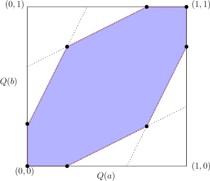
Figure 1: Polytope of reduced form implementable voting rules

The polytope enclosed by these inequalities is shown in Figure 1. One sees 8 extreme points of this polytope, two of them correspond to the constant allocation rules ($(0,0)$ correspond to $b$ always chosen and $(1,1)$ correspond to $a$ always chosen). The rest of them belong to a family of voting rules which we call qualified majority and qualified anti-majority. We establish this result next. This allows us to show that any reduced form implementable voting rule is “equivalent" to a convex combination of voting rules from this set.

Definition 2

Two voting rules $q$ and $\hat{q}$ are reduced form equivalent if they generate the same interim allocation probabilities: $Q(a)=\widehat{Q}(a)$ and $Q(b)=\widehat{Q}(b)$.

We now introduce two classes of voting rules which will be useful to describe the extreme points of reduced form implementable voting rules.

Definition 3

A voting rule $q^{+}$ is a qualified majority if there exists $j\in\{0,\ldots,n\}$ such that for all $k\in\{0,\ldots,n\}$

$$q^{+}(k)=\begin{cases}1&\textrm{if}~{}k\geq j\\ 0&\textrm{otherwise}\end{cases}$$

We call such a voting rule a qualified majority with quota $j$.

A voting rule $q^{-}$ is qualified anti-majority if there exists $j\in\{0,\ldots,n\}$ such that for all $k\in\{0,\ldots,n\}$

$$q^{-}(k)=\begin{cases}1&\textrm{if}~{}k<j\\ 0&\textrm{otherwise}\end{cases}$$

We call such a voting rule a qualified anti-majority with quota $j$.

The definition of qualified majority is similar to Azrieli and Kim (2014). The only difference is that if quota is $j$, they allow $q^{+}(j)$ to take any value in $[0,1]$, but we break the tie deterministically.

If $q^{j}$ is a qualified majority with quota $j$, then its reduced form probabilities are

$$Q^{j}(a) =\frac{1}{n\pi}\sum_{k=0}^{n}kq^{j}(k)B(k)=\frac{1}{n\pi}\sum_{k=j}^{n}kB(k)$$

$$Q^{j}(b) =\frac{1}{n(1-\pi)}\sum_{k=0}^{n}(n-k)q^{j}(k)B(k)=\frac{1}{n(1-\pi)}\sum_{k=j}^{n}(n-k)B(k)$$

Notice that when $j=0$, we have $Q^{0}(a)=Q^{0}(b)=1$. This corresponds to the constant voting rule where $a$ is chosen at every type profile.

If $\bar{q}^{j}$ is a qualified anti-majority with quota $j$, then its reduced form probabilities are

$$\overline{Q}^{j}(a) =\frac{1}{n\pi}\sum_{k=0}^{n}k\bar{q}^{j}(k)B(k)=\frac{1}{n\pi}\sum_{k=0}^{j-1}kB(k)$$

$$\overline{Q}^{j}(b) =\frac{1}{n(1-\pi)}\sum_{k=0}^{n}(n-k)\bar{q}^{j}(k)B(k)=\frac{1}{n(1-\pi)}\sum_{k=0}^{j-1}(n-k)B(k)$$

Denote the set of all qualified majority voting rules by $\mathcal{Q}^{+}$ and the set of all qualified anti-majority voting rules by $\mathcal{Q}^{-}$. Notice that when $j=0$, we have $\overline{Q}^{0}(a)=\overline{Q}^{0}(b)=0$. This corresponds to the constant voting rule where $b$ is chosen at every type profile. Hence, $\mathcal{Q}^{+}\cup\mathcal{Q}^{-}$ contains the two constant voting rules.

Theorem 2

Every symmetric voting rule is reduced-form equivalent to a convex combination of voting rules in $\mathcal{Q}^{+}\cup\mathcal{Q}^{-}$.

We compare our results to some of the results in Azrieli and Kim (2014). They consider a cardinal voting model with two alternatives, where type of an agent (a one-dimensional number with finite support) gives cardinal utilities of two alternatives. They consider cardinal voting rules and Bayesian incentive compatibility (BIC). They have two main results with symmetric cardinal voting rules: (a) a utilitarian maximizer in the class of BIC and symmetric rules is a qualified majority; (b) an interim efficient, BIC and symmetric rule is a qualified majority.

While related, their results and our results are not comparable. First, we only consider ordinal voting rules, while they allow for cardinal rules. Second, the types of agents in their model are independent while we allow for correlated types – exchangeable distributions allow for correlation.

Third, Theorem 2 says that the extreme points of the set of reduced form implementable voting rules consist of qualified majority and qualified anti-majority rules. We do not require incentive compatibility or any additional axiom (like interim efficiency) for this result. In the next section, we will impose monotonicity (equivalent to dominant strategy incentive compatibility) of voting rules, and show that the the extreme points of the set of monotone reduced form implementable voting rules consist of qualified majority rules and a constant rule. As we discuss in Section 4.1, our results are useful in settings where the objective function of the planner is not linear.

Finally, we explore the consequences of imposing unanimity on the reduced form implementation in Section 5. Unanimity is a much weaker axiom than interim efficiency used in Azrieli and Kim (2014). Theorem 5 describes the extreme points of reduced form implementable rules satisfying unanimity and this contains rules that are not qualified majority.

4 Monotone reduced form implementation

A natural restriction on voting rules is monotonicity. Formally, a symmetric voting rule $q$ is monotone if $q(k)\geq q(k-1)$ for all $k\in\{1,\ldots,n\}$. Monotonicity is equivalent to strategy-proofness or dominant strategy incentive compatibility in voting models with two alternatives.

Definition 4

Interim allocation probabilities $Q\equiv(Q(a),Q(b))\in[0,1]^{2}$ is reduced form monotone implementable if there exists a monotone voting rule $q$ whose interim allocation probabilities equal $Q$.

With the help of our main results, we can characterize the reduced form monotone implementable interim allocation probabilities.

Theorem 3

Let $Q\equiv(Q(a),Q(b))$ be any interim allocation probabilities. Then, the following statements are equivalent.

1. $Q$ is reduced form monotone implementable.

2. $Q$ is reduced form implementable and $Q(a)\geq Q(b)$.

3. $Q$ is reduced form implementable by convex combination of qualified majority voting rules and a constant voting rule that selects $b$ at all type profiles.

4. $Q$ satisfies

   $$j(1-\pi)Q(b)-(n-j)\pi Q(a)+\sum_{k=j}^{n}(k-j)B(k) \geq 0\qquad~{}\forall~{}j\in\{0,\ldots,n\}$$ (5)

   $$Q(a)-Q(b) \geq 0$$ (6)

We make two remarks about Theorem 3.

• Equivalence of notions of IC under independent priors. Note that Theorem 3 holds for correlated (exchangeable) priors. The equivalence of (1) and (2) in Theorem 3 is related to equivalence of strategy-proof and Bayesian incentive compatibility in some mechanism design models with independent priors (Manelli and Vincent, 2010; Gershkov, Goeree, Kushnir, Moldovanu, and Shi, 2013). To understand this better, consider a natural notion of Bayesian incentive compatibility in ordinal mechanisms. Ordinal Bayesian incentive compatibility (OBIC) requires that the truthtelling lottery first-order stochastically dominates any lottery that can be obtained by a misreport (d’Aspremont and Peleg, 1988; Majumdar and Sen, 2004; Mishra, 2016).

  Formally, fix a voting rule $q$. Let $Q(x|y)$ denote the interim probability of getting $a$ by reporting $x$ in the voting rule when true type is $y$. So, for an $a$-type agent with utilities $u(a)$ and $u(b)$ for $a$ and $b$ respectively (with $u(a)>u(b)$ since the agent is $a$-type), the IC constraint is

  $$u(a)Q(a|a)+u(b)(1-Q(a|a)) \geq u(a)Q(b|a)+u(b)(1-Q(b|a))$$

  $$\Leftrightarrow(u(a)-u(b))Q(a|a) \geq(u(a)-u(b))Q(b|a)$$

  $$\Leftrightarrow Q(a|a) \geq Q(b|a)$$

  where the last equivalent inequality follows because $u(a)>u(b)$. Similarly, the IC constraint for $b$-type is $1-Q(b|b)\geq 1-Q(a|b)$ or $Q(a|b)\geq Q(b|b)$.

  If prior is independent, then $Q(x|y)=Q(x)$. Then, OBIC is equivalent to requiring $Q(a)\geq Q(b)$. This is the constraint in (2) and (4) of Theorem 3. Hence, by Theorem 3, we have the following corollary.

  Corollary 1

  Suppose the prior is independent and $Q\equiv(Q(a),Q(b))$ be any interim allocation probabilities. Then, each of (1) to (4) in Theorem 3 is equivalent to the following statement

  • $Q$ is reduced form implementable by an OBIC voting rule.

  By the equivalence of (1) and (2) in Theorem 3, Corollary 1 implies that every OBIC voting rule is reduced-form equivalent to a strategy-proof voting rule under independent priors. This OBIC and strategy-proof equivalence result is a corollary of an important (and more general) result on equivalence of strategy-proof and Bayesian incentive compatible mechanism with independent types in Gershkov, Goeree, Kushnir, Moldovanu, and Shi (2013). Corollary 1 describes the reduced form inequalities that characterize OBIC voting rules with independent priors and shows that they are the same reduced form inequalities that describe monotone voting rules.

  In voting models with at least three alternatives, ex-post equivalence of deterministic strategy-proof and OBIC voting rules is established for generic independent priors in Majumdar and Sen (2004) and Mishra (2016) under unanimity constraints.

• Extreme points of voting rules. A voting rule $q$ is extreme if there does not exist a pair of voting rules $\bar{q}$ and $\tilde{q}$ such that for some $\lambda\in(0,1)$, $q(k)=\lambda\bar{q}(k)+(1-\lambda)\tilde{q}(k)$ for all $k$. Let $\mathcal{Q}^{ex}$ be the set of all extreme voting rules.

  A voting rule $q$ is reduced-form extreme if there does not exist a pair of voting rules $\bar{q}$ and $\tilde{q}$ with interim allocation probabilities $\bar{Q}$ and $\tilde{Q}$ respectively, such that for some $\lambda\in(0,1)$, $Q(x)=\lambda\bar{Q}(x)+(1-\lambda)\tilde{Q}(x)$ for all $x\in\{a,b\}$. Let $\mathcal{Q}^{rex}$ be the set of all reduced-form extreme voting rules. By Theorem 2, $\mathcal{Q}^{rex}=\mathcal{Q}^{+}\cup\mathcal{Q}^{-}$.

  It is easy to see that every deterministic voting rule is an extreme voting rule, i.e., belongs to $\mathcal{Q}^{ex}$. For instance, suppose $n=4$, a voting rule that chooses $b$ if there are exactly two $a$-types and chooses $a$ otherwise belongs to $\mathcal{Q}^{ex}$. However this voting rule is neither a qualified majority nor a qualified anti-majority. Hence, it does not belong to $\mathcal{Q}^{rex}$, and hence, we have $\mathcal{Q}^{rex}\subsetneq\mathcal{Q}^{ex}$. That is, the set of extreme points of voting rules in the reduced form is a strict subset of the set of extreme points of voting rules in the ex-post form. This difference disappears once we impose monotonicity.

  To see this, let $\mathcal{Q}^{mex}$ denote the set of monotone extreme voting rules and $\mathcal{Q}^{mrex}$ denote the set of monotone reduced-form extreme voting rules. By Theorem 3, $\mathcal{Q}^{mrex}$ consists of qualified majority voting rules and the constant voting rule that selects $b$ at all type profiles. Picot and Sen (2012) show that $\mathcal{Q}^{mex}$ consists of the same set of voting rules. Hence, we can conclude that $\mathcal{Q}^{mex}=\mathcal{Q}^{mrex}$.

4.1 Application: Rawlsian rule

In this section, we apply Theorem 3 to characterize an ex-ante Rawlsian rule. We say an agent is “satisfied" if its top ranked alternative is chosen. An ex-ante Rawlsian rule maximizes the minimum number of satisfied agents between $a$-types and $b$-types over all monotone voting rules. Formally, fix any voting rule $q$. The expected number of $a$-type satisfied agents is

$$\sum_{k=0}^{n}kq(k)B(k)=n\pi Q(a)$$

Similarly, the expected number of $b$-type satisfied agents is

$$\sum_{k=0}^{n}(n-k)(1-q(k))B(k)=n(1-\pi)(1-Q(b))$$

An ex-ante Rawlsian rule maximizes the minimum number of satisfied agents between $a$-types and $b$-types.

Definition 5

A monotone voting rule $q^{R}$ is ex-ante Rawlsian if for every monotone voting rule $q$,

$$\min\big{(}\pi Q^{R}(a),(1-\pi)(1-Q^{R}(b)\big{)} \geq\min\big{(}\pi Q(a),(1-\pi)(1-Q(b)\big{)}$$

Using Theorem 3, we provide a complete description of the ex-ante Rawlsian rule: it is a convex combination of a pair of qualified majority voting rules.

Proposition 1

The ex-ante Rawlsian rule $q^{R}$ is a convex combination of qualified majority with quota $j^{*}$ and $(j^{*}+1)$, where

$$j^{*}=\max\{j\in\{0,\cdots,n\}:\sum_{k=j}^{n}B(k)\geq 1-\pi\}$$ (7)

The interim allocation probabilities corresponding to $q^{R}$ are

$$Q^{R}(a) =\frac{1}{n\pi}\left(j^{*}(1-\pi)+\sum_{k=j^{*}}^{n}(k-j^{*})B(k)\right)$$ (8)

$$Q^{R}(b) =\frac{1}{n(1-\pi)}\left((n-j^{*})(1-\pi)-\sum_{k=j^{*}}^{n}(k-j^{*})B(k)\right)$$ (9)

The optimal quota $j^{*}$ is determined by comparing the joint probability that at least $j^{*}$ agents is $a$-type and the marginal probability of $b$-type (which is $1-\pi$). For qualified majority with quotas $j^{*}$ and $j^{*}+1$, the joint probability that at least $j^{*}$ agents is $a$-type is approximately equal to the ex ante probability that alternative $a$ is chosen from these rules. Then optimal quota $j^{*}$ is selected such that the ex ante probability that alternative $a$ is chosen is approximately equal to the marginal probability of $b$-type.

5 Unanimity constraints

We now impose a familiar axiom on the voting rule. A voting rule $q$ is unanimous if $q(n)=1$ and $q(0)=0$. Unanimity imposes restrictions on the interim allocation probabilities. For instance, consider a unanimous voting rule $q$. Then, its interim allocation probabilities must be

$$Q(a) =\frac{1}{n\pi}\sum_{k=0}^{n}kq(k)B(k)=\frac{1}{n\pi}\big{[}\sum_{k=1}^{n-1}kq(k)B(k)+nB(n)\big{]}$$

$$Q(b) =\frac{1}{n(1-\pi)}\sum_{k=1}^{n-1}(n-k)q(k)B(k)$$

Hence, the reduced-form characterization changes as in the theorem below.

Definition 6

Interim allocation probabilities $Q(a),Q(b)\in[0,1]$ is reduced form unanimous (u-)implementable if there exists a unanimous voting rule $q$ whose interim allocation probabilities equal $Q$.

Notice that $q$ is $(n-2)$-dimensional since the values of $q(0)$ and $q(n)$ are fixed.

Theorem 4

Interim allocation probabilities $Q$ is reduced form u-implementable if and only if

$$j(1-\pi)Q(b)-(n-j)\pi Q(a)+\sum_{k=j}^{n}(k-j)B(k) \geq 0\qquad~{}\forall~{}j\in\{0,\ldots,n\}$$ (10)

$$(n-j)\pi Q(a)-j(1-\pi)Q(b)+\sum_{k=0}^{j}(j-k)B(k) \geq j\lambda(0)+(n-j)\lambda(n)\qquad~{}\forall~{}j\in\{0,\ldots,n\}$$ (11)

The proofs of Theorem 4 and Theorem 5 are in Appendix B. They are similar to Theorem 1 and Theorem 2.

For $n=3$ and the uniform prior with $\pi=\frac{1}{2}$, the set of reduced form u-implementable voting rules are shown in the smaller polytope in Figure 2. It lies inside the polytope characterizing the set of all reduced form implementable voting rules. This polytope has only four extreme points. We characterize them next.

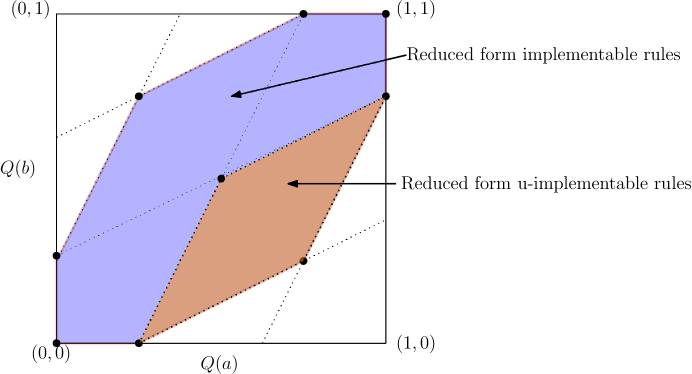
Figure 2: Polytope of reduced form u-implementable voting rules

The extreme points of reduced-form implementable unanimous voting rules are defined by two new families of unanimous voting rules.

Definition 7

A voting rule $q^{+}_{u}$ is u-qualified majority if it is a qualified majority with quota $j$, where $j\in\{1,\ldots,n\}$. We call such a voting rule a u-qualified majority with quota $j$.

A voting rule $q^{-}_{u}$ is u-qualified anti-majority if there exists $j\in\{1,\ldots,n\}$

$$q^{-}_{u}(k)=\begin{cases}1&\textrm{if}~{}k\in\{1,\ldots,j-1\}\cup\{n\}\\ 0&\textrm{otherwise}\end{cases}$$

We call such a voting rule a u-qualified anti-majority with quota $j$.

A u-qualified majority is just a non-constant qualified majority rule. On the other hand, a u-qualified anti-majority is not merely a non-constant qualified anti-majority. A u-qualified anti-majority is constructed by taking a non-constant qualified anti-majority and making it unanimous. For instance if $n=4$ and quota $j=2$, a qualified anti-majority will set $q(0)=q(1)=1,q(2)=q(3)=q(4)=0$. But a u-qualified anti-majority will set $q(0)=0,q(1)=1,q(2)=q(3)=0,q(4)=1$.

We write down the interim allocation probabilities of a u-qualified majority and u-qualified anti-majority below. If $q^{+}_{u}$ is a u-qualified majority with quota $j$, then

$$Q^{+}_{u}(a) =\frac{1}{n\pi}\sum_{k=j}^{n}kB(k)$$

$$Q^{+}_{u}(b) =\frac{1}{n(1-\pi)}\sum_{k=j}^{n}(n-k)B(k)$$

On the other hand, if $q^{-}_{u}$ is a u-qualified anti-majority with quota $j$, then

$$Q^{-}_{u}(a) =\frac{1}{n\pi}\Big{[}\sum_{k=1}^{j-1}kB(k)+nB(n)\Big{]}$$

$$Q^{-}_{u}(b) =\frac{1}{n(1-\pi)}\sum_{k=1}^{j-1}(n-k)B(k)$$

Denote the set of all u-qualified majority voting rules by $\mathcal{Q}_{u}^{+}$ and the set of all u-qualified anti-majority voting rules by $\mathcal{Q}_{u}^{-}$. Notice that the u-qualified majority with quota $n$ and the u-qualified anti-majority with quota $1$ are the same voting rules. Similarly, the u-qualified majority with quota $1$ and the u-qualified anti-majority with quota $n$ are the same voting rules. Hence, these two families of voting rules contain a total of $2(n-1)$ unanimous voting rules. The following theorem shows that they form the extreme points of all reduced form u-implementable voting rules.

Theorem 5

Every symmetric and unanimous voting rule is reduced-form equivalent to a convex combination of voting rules in $\mathcal{Q}_{u}^{+}\cup\mathcal{Q}_{u}^{-}$.

5.1 When are incentive constraints implied?

Corollary 1 (and Gershkov, Goeree, Kushnir, Moldovanu, and Shi (2013)) shows that for independent priors, every OBIC voting rule is reduced form equivalent to a strategy-proof voting rule. This reduced form equivalence, however, fails with unanimity constraint, i.e., not every OBIC and unanimous voting rule is reduced form equivalent to a strategy-proof and unanimous voting rule. The following example presents an OBIC and unanimous voting rule that is not reduced form equivalent to a strategy-proof and unanimous voting rule.

Example 1

Suppose $n=3$ and the prior is independent with $\pi=\frac{1}{2}$: so, $B(0)=\frac{1}{8},B(1)=\frac{3}{8},B(2)=\frac{3}{8},B(3)=\frac{1}{8}$. Consider $Q(a)=Q(b)=\frac{1}{2}$. Then $Q$ is OBIC. We show that $Q$ is implementable by a unique unanimous voting rule, but it is not strategy-proof. Let $q$ be any unanimous rule that implements $Q$. Then $q$ satisfies

$$Q(a) =\frac{1}{3\pi}[\sum_{k=1}^{2}kq(k)B(k)+3B(3)]=\frac{1}{4}\Big{(}q(1)+2q(2)+1\Big{)}=\frac{1}{2}$$

$$Q(b) =\frac{1}{3\pi}\sum_{k=1}^{2}(3-k)q(k)B(k)=\frac{1}{4}\Big{(}2q(1)+q(2)\Big{)}=\frac{1}{2}$$

Hence $q(1)-q(2)=1$. Since $0\leq q(1),q(2)\leq 1$, it implies that $q(1)=1$ and $q(2)=0$, i.e., $q$ is unique. However, $q$ is not strategy-proof. $\blacksquare{}$

Imposing unanimity contracts the set of reduced form implementable voting rules. In contrast to qualified anti-majority rules, some u-qualified anti-majority rules can be OBIC. The following result provides a necessary and sufficient condition on prior beliefs such that all unanimous voting rules are OBIC.

Proposition 2

Every unanimous and symmetric voting rule is OBIC if and only if

$$\lambda(j) \leq\min\Big{(}\frac{\lambda(1)+\lambda(n)}{C(n-1,j-1)},\frac{\lambda(0)+\lambda(n-1)}{C(n-1,j)}\Big{)}\qquad~{}\forall~{}j\in\{1,\ldots,n-1\}$$ (12)

Further, if the prior is independent, every unanimous and symmetric voting rule is OBIC if and only if

$$C(n-1,j-1) \leq\Big{[}\Big{(}\frac{\pi}{1-\pi}\Big{)}^{n-j}+\Big{(}\frac{\pi}{1-\pi}\Big{)}^{1-j}\Big{]}~{}\qquad~{}\forall~{}j\in\{1,\ldots,n-1\}$$ (13)

Using Corollary 1, we can argue that when (13) holds and the prior is independent, every unanimous voting rule is reduced form equivalent to a strategy-proof voting rule. An immediate corollary of the above result is that when there is a small number of agents, every unanimous voting rule is OBIC if the prior is independent.

Corollary 2

If the prior is independent and $n=3$, every unanimous and symmetric voting rule is OBIC.

Proof:  Since $\pi\in(0,1)$, $j^{*}=\lfloor 3\pi\rfloor\leq 2$. If $j^{*}=1$, we get

$$B(1)=3\pi(1-\pi)^{2} \leq 3\pi(\pi^{2}+(1-\pi)^{2})$$

If $j^{*}=2$, we get

$$B(2)=3\pi^{2}(1-\pi)=\frac{3\pi}{2}(2\pi(1-\pi))\leq\frac{3\pi}{2}(\pi^{2}+(1-\pi)^{2})$$

Hence, by Proposition 2, every unanimous voting rule is OBIC. $\blacksquare{}$

To illustrate Proposition 2, suppose $n=4$. The condition (12) is given by

$$3\lambda(2)\leq\lambda(1)+\lambda(4)$$

$$3\lambda(3)\leq\lambda(1)+\lambda(4)$$

$$3\lambda(1)\leq\lambda(0)+\lambda(3)$$

$$3\lambda(2)\leq\lambda(0)+\lambda(3)$$

Notice that for independent uniform priors, $\lambda(k)=(\frac{1}{2})^{4}$, the belief conditions fail. For sufficiently positively correlated beliefs where $\lambda(0)$ and $\lambda(4)$ are large, the belief conditions hold. This is in general true. If $\lambda(0)$ and $\lambda(n)$ are sufficiently large, (12) holds. Similarly, if $\lambda(0)$ and $\lambda(1)$ (or, $\lambda(n-1)$ and $\lambda(n)$) are sufficiently large, (12) holds.

6 Large Economies

In this section, we apply our results to large economies. For this, we assume independent and identically distributed types. So, $\pi$ denotes the probability that an agent is $a$-type. Let $\mu:=n\pi$ denote the mean of the binomial distribution.

There are two ways in which we increase the value of $n$. First, we fix the value of $\pi$ and increase $n$. This implies that the expected number of $a$-types ($\mu$) also increases. Second, we fix the expected number of $a$-types at $\mu$, and increase $n$. This implies that the value of $\pi$ decreases with increasing $n$. We show the implication of large $n$ on the set of reduced form implementable voting rules in both the cases.

Since $n$ is variable in this section, for an arbitrary voting rule, we denote the interim allocation probabilities as $(Q(a;n),Q(b;n))$ in this section. For a fixed $\pi$ and $n$, the interim allocation probabilities corresponding to qualified majority and anti-qualified majority voting rules will be useful for our analysis. In particular, pick a qualified majority voting rule with quota $j>0$. For such a qualified majority, the interim allocation probabilities satisfy

$$Q^{j}(a;n)-Q^{j}(b;n) =\frac{1}{n\pi}\sum_{k=j}^{n}kB(k)-\frac{1}{n(1-\pi)}\sum_{k=j}^{n}(n-k)B(k)$$

$$=\frac{1}{n\pi}\sum_{k=j}^{n}kC(n,k)\pi^{k}(1-\pi)^{(n-k)}-\frac{1}{n(1-\pi)}\sum_{k=j}^{n}(n-k)C(n,k)\pi^{k}(1-\pi)^{(n-k)}$$

$$=\sum_{k=j}^{n}C(n-1,k-1)\pi^{k-1}(1-\pi)^{(n-k)}-\sum_{k=j}^{n}C(n-1,k)\pi^{k}(1-\pi)^{(n-k-1)}$$

$$=C(n-1,j-1)\pi^{j-1}(1-\pi)^{(n-j)}$$ (14)

Similarly, for a qualified anti-majority with quota $j>0$, the interim allocation probabilities satisfy

$$\overline{Q}^{j}(b;n)-\overline{Q}^{j}(a;n) =C(n-1,j-1)\pi^{j-1}(1-\pi)^{(n-j)}$$ (15)

This can also be seen from the fact that for a fixed quota $j$, the qualified majority and the qualified anti-majority interim allocation probabilities are related as: $\overline{Q}^{j}(a;n)=1-Q^{j}(a;n)$ and $\overline{Q}^{j}(b;n)=1-Q^{j}(b;n)$.

Depending on whether we increase $n$ for a fixed $\pi$ or fixed $\mu$, the RHS of (14) (and (15)) behaves differently. In the former case, it is approximately equal to a normal distribution with vanishing values of density. In the latter case, it is related to the Poisson distribution. This leads to different convergence results in these cases.

Proposition 3

Suppose $\pi$ is fixed and $\pi\in(0,1)$. Then, for every $\epsilon>0$, there exists $n_{0}$ such that for every $n$-agent economy with $n>n_{0}$, if interim allocation $(Q(a,n),Q(b,n))$ is reduced form implementable, then

$$|Q(a;n)-Q(b;n)|<\epsilon.$$

Proposition 3 says that in large economies, the only reduced form implementable probabilities are those where $Q(a;n)=Q(b;n)$. If the number of agents is large, the interim allocation probabilities (for any voting rule) is less sensitive to the type of the agent. Hence, both $a$-types and $b$-types get the same interim allocation probabilities with large $n$.

However, this is not the case if the economies become large with a fixed $\mu$. If $\mu$ is fixed, increasing $n$ decreases $\pi$. So, the probability of $a$-types decreases, i.e., $b$-types dominate the economy. As a result, depending on how sensitive a voting rule is to the number of $b$-types (or $a$-types), we may get quite different interim allocation probabilities $Q(a;n)$ and $Q(b;n)$. For instance, consider the simple rule that chooses $b$ when all agents have $b$-type and chooses $a$ otherwise. Then, if an agent has $a$-type, the rule must choose: $Q(a;n)=1$. But if an agent has $b$-type, the rule chooses $b$ if all other $(n-1)$ agents have $b$ type. For a fixed $\mu$, the probability that a given agent has $b$ type is $1-(\mu/n)$. So, probability that $(n-1)$ agents have $b$ type is $\big{(}1-(\mu/n)\big{)}^{n-1}$, which converges to $e^{-\mu}$ for large $n$. So, for large $n$, we have $Q(b;n)=1-e^{-\mu}$, and $Q(a;n)-Q(b;n)=e^{-\mu}>0$. The proposition below uses a slightly more sophisticated voting rule to come up with an improved bound on $Q(a;n)-Q(b;n)$.

Proposition 4

Suppose $\mu$ is fixed. Then, there is a positive constant $M(\mu)$ such that for every $\epsilon>0$, there exists $n_{0}$ such that for every $n$-agent economy with $n>n_{0}$,

1. interim allocation probabilities $(Q(a,n),Q(b,n))$ exists which is reduced form implementable and

   $$Q(a;n)-Q(b;n)>M(\mu)-\epsilon$$

2. interim allocation probabilities $(\widehat{Q}(a;n),\widehat{Q}(b;n))$ exists which is reduced form implementable and

   $$\widehat{Q}(b;n)-\widehat{Q}(a;n)>M(\mu)-\epsilon$$

Combining Propositions (3), (4) and Corollary (1), we conclude that every reduced form implementable rule is strategy-proof in the large for the fixed $\pi$, but this is not the case if $\mu$ is fixed.

7 Relation to the literature

The Border’s theorem for single object allocation problem was formulated in Matthews (1984); Maskin and Riley (1984). The reduced form characterization for this problem were developed in Border (1991). The symmetric version of Border’s theorem with an elegant proof using Farkas Lemma is developed in Border (2007). There are other approaches to proving Border’s theorem (which also makes it applicable in some constrained environment): network flow approach in Che, Kim and Mierendorff (2013), geometric approach in Goeree and Kushnir (2022). Hart and Reny (2015) provide an equivalence characterization of Border’s theorem using second order stochastic dominance. Kleiner, Moldovanu and Strack (2021) further develop the majorization approach and apply it to a variety of problems in economics. Border’s theorem applies to private values single object auction, but Goeree and Kushnir (2016) extend Border’s theorem to allow for value interdependencies. Zheng (2021) generalizes reduced-form characterizations to allocation of multiple objects with paramodular constraints. Lang and Yang (2021) study a universal implementation for allocation of multiple objects. Yang (2021) considers the consequences of incorporating fairness constraints in the reduced form problem. Lang (2022) considers a public good allocation problem but with only two agents (but multiple alternatives). He provides an extension of Border’s theorem to his two-agent problem. Our ordinal voting model over two alternatives is a public good model with a specific type space, which is not covered in these papers.

Vohra (2011) studies the combinatorial structure of reduced-form auctions by the polymatroid theory; see also Che, Kim and Mierendorff (2013), Alaei, Fu, Haghpanah, Hartline, and Malekian (2019) and Zheng (2021). Our characterization condition shares some similarity with a polymatroid as it requires only integer valued coefficients in linear inequalities. At the same time, it differs from a polymatroid in that the inequalities contain not only 0,1 coefficients but more general integer coefficients.

The two alternatives voting model has received attention in the literature in social choice theory – from May’s theorem (May, 1952) to its extensions, including a recent extension by Bartholdi, Josyula, Tamuz, and Yariv (2021). Schmitz and Tröger (2012) identify qualified majority rules as ex-ante welfare maximizing in the class of dominant strategy voting rules. The results in Azrieli and Kim (2014) (which we discussed earlier) show that focusing attention to ordinal rules in this model is without loss of generality in a certain sense – see Nehring (2004) also.

Appendix A Missing proofs

We first prove Theorem 2, and then Theorem 1.

A.1 Proof of Theorem 2

Proof:  Reduced form probabilities $(Q(a),Q(b))$ is implementable if

$$\frac{1}{n\pi}\sum_{k=0}^{n}kq(k)B(k) =Q(a)$$ (16)

$$\frac{1}{n(1-\pi)}\sum_{k=0}^{n}(n-k)q(k)B(k) =Q(b)$$ (17)

$$0\leq q(k) \leq 1\qquad~{}\forall~{}k\in\{0,1,\ldots,n\}$$ (18)

Let $\mathcal{P}$ be the projection of this polytope onto the $(Q(a),Q(b))$-space. Clearly, $\mathcal{P}$ is a polytope. Consider the following linear program

$$\max_{Q}\mu_{a}Q(a)+\mu_{b}Q(b)$$ (LP-Q)

$$\textrm{subject to}~{}~{}~{}(Q(a),Q(b))~{}\in\mathcal{P}$$

As we vary $\mu_{a}$ and $\mu_{b}$, the solutions to the linear program program (LP-Q) characterize the boundary points of $\mathcal{P}$. Since each point in $\mathcal{P}$ is equivalent to finding a voting rule $q$ that satisfies (16), (17), and (18), we can rewrite the linear program (LP-Q) in the space of $q$ as:

$$\max_{q}\Big{[}\frac{\mu_{a}}{n\pi}\sum_{k=0}^{n}kq(k)B(k) +\frac{\mu_{b}}{n(1-\pi)}\sum_{k=0}^{n}(n-k)q(k)B(k)\Big{]}$$ (LP-q)

$$\textrm{subject to}~{}~{}~{}0\leq q(k) \leq 1\qquad~{}\forall~{}k\in\{0,1,\ldots,n\}$$

Hence, the set of boundary points of $\mathcal{P}$ can be described by the interim allocation probabilities of the voting rules obtained as a solution to the linear program (LP-q) as we vary $\mu_{a}$ and $\mu_{b}$.

We now do the proof in two steps.

Step 1. We first show that every extreme point of $\mathcal{P}$ is implemented by either a qualified majority voting rule or a qualified anti-majority voting rule, i.e., every element of $\mathcal{P}$ can be written as a convex combination of qualified (anti-)majority voting rules.

It is sufficient to show that for every $\mu_{a}$ and $\mu_{b}$, there is a solution to (LP-Q) that is implemented by either a qualified majority or a qualified anti-majority voting rule. To show this, we show that for every $\mu_{a}$ and $\mu_{b}$, some qualified (anti-)majority voting rule is a solution to (LP-q).

By denoting $\hat{\mu}_{a}:=\mu_{a}/(n\pi)$ and $\hat{\mu}_{b}:=\mu_{b}/(n(1-\pi))$, we see that the objective function of (LP-q) is

$$\sum_{k=0}^{n}\big{[}n\hat{\mu}_{b}+k(\hat{\mu}_{a}-\hat{\mu}_{b})\big{]}q(k)B(k)$$

We show that $n\hat{\mu}_{b}+k(\hat{\mu}_{a}-\hat{\mu}_{b})$ is either weakly increasing, in which case some qualified majority voting rule is optimal) or weakly decreasing, in which case some qualified anti-majority voting rule is optimal.

If $n\hat{\mu}_{b}+k(\hat{\mu}_{a}-\hat{\mu}_{b})>0$ for all $k$, then a solution to (LP-q) is to set $q(k)=1$ for all $k$. This is the qualified majority with quota $0$. If $n\hat{\mu}_{b}+k(\hat{\mu}_{a}-\hat{\mu}_{b})<0$ for all $k$, then a solution to (LP-q) is to set $q(k)=0$ for all $k$. This is the qualified anti-majority with quota $0$. If $n\hat{\mu}_{b}+k(\hat{\mu}_{a}-\hat{\mu}_{b})=0$ for all $k$, then every voting rule $q$ is a solution.

If the sign of $n\hat{\mu}_{b}+k(\hat{\mu}_{a}-\hat{\mu}_{b})$ changes with $k$, then we consider two cases. If $\hat{\mu}_{a}>\hat{\mu}_{b}$, then there is a cut-off $k^{*}$ such that $n\hat{\mu}_{b}+k(\hat{\mu}_{a}-\hat{\mu}_{b})>0$ for all $k\geq k^{*}$ and $n\hat{\mu}_{b}+k(\hat{\mu}_{a}-\hat{\mu}_{b})<0$ for all $k<k^{*}$. Then, the qualified majority with quota $k^{*}$ is a solution to (LP-q). On the other hand if $\hat{\mu}_{a}<\hat{\mu}_{b}$, then there is a cutoff $k^{*}$ such that $n\hat{\mu}_{b}+k(\hat{\mu}_{a}-\hat{\mu}_{b})>0$ for all $k\leq k^{*}$ and $n\hat{\mu}_{b}+k(\hat{\mu}_{a}-\hat{\mu}_{b})<0$ for all $k>k^{*}$. Then, the qualified anti-majority with quota $k^{*}$ is a solution of (LP-q). Note that in both cases above, if $n\hat{\mu}_{b}+k(\hat{\mu}_{a}-\hat{\mu}_{b})=0$ for $k=k^{*}$, the (anti-)qualified majority with quota $k^{*}$ is a solution to (LP-q).

Step 2. We now show that every qualified (anti-)majority voting rule implements a distinct extreme point of $\mathcal{P}$. Every extreme point in $\mathcal{P}$ is obtained by considering values of $\mu_{a}$ and $\mu_{b}$ which generate a unique optimal solution to the linear program (LP-Q). It is sufficient to show that every qualified (anti-)majority voting rule is unique optimal solution to (LP-q) for some $\mu_{a}$ and $\mu_{b}$. This is easily seen from our analysis above that for almost all $\mu_{a}$ and $\mu_{b}$, in case an optimal solution to (LP-q) exists, it is unique, corresponds to a qualified majority or a qualified anti-majority voting rule.

Combining Steps 1 and 2, we see that the set of extreme points of $\mathcal{P}$ is the set of qualified majority voting rules and the set of qualified anti-majority voting rules. $\blacksquare{}$

A.2 Proof of Theorem 1

Proof:  We know that the necessary conditions for reduced form implementation are (3) and (4). Let $\mathcal{P}^{*}$ denote the polytope described by (3) and (4). We show that the extreme points of $\mathcal{P}^{*}$ correspond to the qualified majority and the qualified anti-majority voting rules. From Theorem 2, we know that the extreme points of $\mathcal{P}$ also correspond to the qualified majority and the qualified anti-majority voting rules. Hence, $\mathcal{P}=\mathcal{P}^{*}$.

To show that the extreme points of $\mathcal{P}^{*}$ correspond to the qualified majority and the qualified anti-majority voting rules, we follow two steps.

Every $q\in\mathcal{Q}^{+}\cup\mathcal{Q}^{-}$ is an extreme point. Consider any qualified majority voting rule with quota $j\in\{1,\ldots,n\}$. Using

$$n\pi Q^{j}(a)=\sum_{k=j}^{n}kB(k)~{}~{}~{}\textrm{and}~{}~{}n(1-\pi)Q^{j}(b)=\sum_{k=j}^{n}(n-k)B(k),$$

it is easy to verify that $Q^{j}$ satisfies all inequalities in $(\ref{eq:e1})$ and $(\ref{eq:e2})$ and inequality (3) is binding for $j$ and $(j-1)$ at $Q^{j}$. Since $Q^{j}\in\mathcal{P}^{*}$ and $Q^{j}$ is the intersection of two linearly independent hyperplanes, it gives an extreme point of $\mathcal{P}^{*}$. Since the qualified majority voting rule with quota $0$ corresponds to a constant voting rule, that is also an extreme point.

An analogous argument shows that the interim allocation probability of every qualified anti-majority voting rule with a quota $j\in\{0,\ldots,n\}$ is an extreme point.

No extreme point outside $\mathcal{Q}^{+}\cup\mathcal{Q}^{-}$. Consider an extreme point of $\mathcal{P}^{*}$ that is not a qualified (anti-)majority rule. Then two non-adjacent constraints must be binding, i.e., either (3) binds for some $j$ and $j+\ell$ with $\ell>1$, or (4) binds for some $j$ and $j+\ell$ with $\ell>1$, or (3) binds for some $j$ and (4) binds for some $\ell$.

Assume first that (3) binds for $j$ and $j+\ell$, where $\ell>1$. The equality corresponding to $(j+\ell)$ is

$$0 =(j+\ell)(1-\pi)Q(b)-(n-j-\ell)\pi Q(a)+\sum_{k=j+\ell+1}^{n}(k-j-\ell)B(k)$$

$$=\ell\Big{(}\pi Q(a)+(1-\pi)Q(b)\Big{)}+j(1-\pi)Q(b)-(n-j)\pi Q(a)$$

$$+\sum_{k=j+\ell+1}^{n}(k-j)B(k)-\sum_{k=j+\ell+1}^{n}\ell B(k)$$

Since inequality (3) binds for $j$, substitute the equality into (3) for $j+1$,

$$\pi Q(a)+(1-\pi)Q(b)\geq\sum_{k=j+1}^{n}B(k)$$

We get

$$0 \geq\sum_{k=j+1}^{n}\ell B(k)-\sum_{k=j+\ell+1}^{n}\ell B(k)+\sum_{k=j+\ell+1}^{n}(k-j)B(k)-\sum_{k=j+1}^{n}(k-j)B(k)$$

$$=\sum_{k=j+1}^{j+\ell}\ell B(k)-\sum_{k=j+1}^{j+\ell}(k-j)B(k)=\sum_{k=j+1}^{j+\ell}(j+\ell-k)B(k)>0$$

which is a contradiction. Hence, (3) cannot bind for $j$ and $(j+\ell)$ for $\ell>1$. An analogous proof shows that (4) cannot bind for $j$ and $(j+\ell)$ for $\ell>1$.

Now, assume (3) binds for $j$ and (4) binds for $\ell$. Hence, adding those two equalities, we get

$$0 =(j-\ell)(1-\pi)Q(b)+(j-\ell)\pi Q(a)+\sum_{k=0}^{\ell-1}(\ell-k)B(k)+\sum_{k=j+1}^{n}(k-j)B(k)$$

If $j\geq\ell$ and $(j,\ell)\neq(n,0)$, the RHS is positive, giving us a contradiction. If $j<\ell$ and $(j,\ell)\neq(0,n)$, using $\pi Q(a)+(1-\pi)Q(b)\leq 1$, we get

$$0 =(j-\ell)\Big{(}(1-\pi)Q(b)+\pi Q(a)\Big{)}+\sum_{k=0}^{\ell-1}(\ell-k)B(k)+\sum_{k=j+1}^{n}(k-j)B(k)$$

$$\geq j-\ell+\sum_{k=0}^{\ell-1}(\ell-k)B(k)+\sum_{k=j+1}^{n}(k-j)B(k)$$

$$=j\Big{(}1-\sum_{k=j+1}^{n}B(k)\Big{)}-\ell\Big{(}1-\sum_{k=0}^{\ell-1}B(k)\Big{)}+\Big{(}\sum_{k=\ell}^{n}kB(k)-n\pi\Big{)}+\Big{(}n\pi-\sum_{k=0}^{j}kB(k)\Big{)}$$

$$=\sum_{k=0}^{j}(j-k)B(k)+\sum_{k=\ell}^{n}(k-\ell)B(k)>0$$

which also gives us a contradiction.

If $(j,\ell)=(n,0)$ or $(0,n)$, the two equalities determine $(Q(a),Q(b))=(0,0)$ or $(1,1)$, which correspond to the two constant voting rules, which are in $\mathcal{Q}^{+}\cap\mathcal{Q}^{-}$. $\blacksquare{}$

A.3 Proof of Theorem 3

Proof:  $(1)\Rightarrow(2)$. Since $Q$ is reduced form monotone implementable, it is reduced form implementable by a monotone voting rule $q$. Hence, we can write

$$n\pi(1-\pi)\Big{[}Q(a)-Q(b)\Big{]} =\sum_{k=0}^{n}\big{[}k(1-\pi)-(n-k)\pi\big{]}q(k)B(k)=\sum_{k=0}^{n}(k-n\pi)q(k)B(k)$$

$$\geq q(\lfloor n\pi\rfloor)\sum_{k=0}^{n}(k-n\pi)B(k)=0$$

where we use monotonicity of $q$ for the inequality. This shows $Q(a)\geq Q(b)$.

$(2)\Rightarrow(3)$. If $Q$ is reduced form implementable, by Theorem 2, it can be expressed as convex combination of interim allocation probabilities of qualified majority and qualified anti-majority voting rules.

Consider any qualified anti-majority with quota $j\in\{0,\ldots,n\}$ (qualified anti-majority with quota $0$ corresponds to a constant voting rule). Define for each $j\in\{0,\ldots,n\}$

$$\delta(j):=\overline{Q}^{j}(a)-\overline{Q}^{j}(b) =\frac{1}{n\pi}\sum_{k=0}^{j-1}kB(k)-\frac{1}{n(1-\pi)}\sum_{k=0}^{j-1}(n-k)B(k)=\frac{1}{n\pi(1-\pi)}\sum_{k=0}^{j-1}(k-n\pi)B(k)$$

Note that $\delta(0)=0$ and $\delta(n)=-n(1-\pi)B(n)<0$.

For all $j\in\{0,\ldots,n-1\}$, we get

$$\delta(j+1)-\delta(j) =\frac{1}{n\pi(1-\pi)}(j-n\pi)B(j)$$

which is non-negative if $j\geq n\pi$ and negative if $j<n\pi$. Hence, value of $\delta(j)$ decreases with $j$ for all $j<n\pi$ and increases after that till $j=n$. Since $\delta(0)=0$ and $\delta(n)<0$, we conclude that $\delta(j)=\overline{Q}^{j}(a)-\overline{Q}^{j}(b)<0$ for all $j\in\{1,\ldots,n\}$ and $\delta(0)=0$.

On the other hand, for any qualified majority with quota $j$, we have $Q^{j}(a)\geq Q^{j}(b)$. The qualified anti-majority with quota zero corresponds to a constant voting rule which generates interim allocation probabilities $Q(a)=Q(b)=0$. Hence, if $Q(a)\geq Q(b)$, then $Q$ is reduced form implementable by convex combination of qualified majority voting rules and a constant voting rule that selects $b$ at all type profiles.

$(3)\Rightarrow(4)$. Every qualified majority and qualified anti-majority with quota zero generates interim allocation probabilities $Q$ that satisfy $Q(a)\geq Q(b)$. Hence, their convex combination also satisfies $Q(a)\geq Q(b)$. By Theorem 1, if $Q$ is reduced form implementable then it satisfies (5).

$(4)\Rightarrow(1)$. The proof of Theorem 1 shows that the set of extreme points of (5) is the set of qualified majority voting rules. The line $Q(a)=Q(b)$ connects two constant voting rules and all the qualified majority voting rules satisfy $Q(a)\geq Q(b)$. As a result, any $Q$ satisfying (5) and (6) must be reduced-form equivalent to a convex combination of qualified majority voting rules and the two constant voting rules. Hence, it is reduced form monotone implementable. $\blacksquare{}$

A.4 Proof of Proposition 1

Proof:  By Theorem 3, the ex-ante Rawlsian rule solves the following optimization problem

$$\max_{Q}\min\big{(}\pi Q(a),(1-\pi)(1-Q(b)\big{)}$$

$$\textrm{subject to}~{}~{}~{}~{}Q(a) \geq Q(b)$$ (19)

$$j(1-\pi)Q(b)-(n-j)\pi Q(a)+\sum_{k=j}^{n}(k-j)B(k) \geq 0~{}\qquad~{}\forall~{}j\in\{0,\ldots,n\}$$ (20)

Consider the relaxed problem where we drop the inequalities in (19). Further, change the variables as follows: $x:=\pi Q(a)$ and $y:=(1-\pi)(1-Q(b))$. So, the relaxed problem (with inequalities (19) in terms of $x,y$) is the following

$$\max_{x,y}\min\big{(}x,y\big{)}$$

$$\textrm{subject to}~{}~{}~{}~{}jy+(n-j)x \leq j(1-\pi)+\sum_{k=j}^{n}(k-j)B(k)~{}\qquad~{}\forall~{}j\in\{0,\ldots,n\}$$ (21)

Notice that for any feasible solution $(x,y)$ to the above problem, the solution $\hat{x}=\hat{y}=\min(x,y)$ is also a feasible solution with the same objective function value. Hence, it is without loss of generality to assume $x=y$. Hence, substituting $x=y$ on the LHS of (21), we get $nx$, and the problem simplifies to

$$\max_{x}x$$

$$\textrm{subject to}~{}~{}nx \leq j(1-\pi)+\sum_{k=j}^{n}(k-j)B(k)~{}\qquad~{}\forall~{}j\in\{0,\ldots,n\}$$ (22)

For every $j\in\{0,\ldots,n\}$, let $H(j):=j(1-\pi)+\sum_{k=j}^{n}(k-j)B(k)$. Hence, the optimal solution is given by

$$x=y =\frac{1}{n}\min_{j\in\{0,\ldots,n\}}H(j)$$

For $j\in\{1,\ldots,n\}$, we see

$$H(j)-H(j-1)=1-\pi-\sum_{k=j}^{n}B(k)$$

Let $j^{*}:=\max\{j\in\{0,\cdots,n\}:\sum\limits_{k=j}^{n}B(k)\geq 1-\pi\}$. Then, $H$ is decreasing till $j^{*}$ and increasing after that. So, $x=y=(1/n)H(j^{*})$ is an optimal solution to the relaxed problem. This optimal solution corresponds to

$$Q(a) =\frac{1}{n\pi}\Big{[}j^{*}(1-\pi)+\sum_{k=j^{*}}^{n}(k-j^{*})B(k)\Big{]}$$

$$Q(b) =\frac{1}{n(1-\pi)}\Big{[}(n-j^{*})(1-\pi)-\sum_{k=j^{*}}^{n}(k-j^{*})B(k)\Big{]}$$

This corresponds to satisfying inequality (22) for $j^{*}$.

Now, define

$$\alpha:=\frac{1}{B(j^{*})}\left(1-\pi-\sum_{k=j^{*}+1}^{n}B(k)\right)$$

By definition of $j^{*}$, $\alpha\in[0,1]$. Using the expressions for $Q^{j^{*}}(a)$ and $Q^{j^{*}+1}(a)$, it can be easily verified that

$$Q(a)=\alpha Q^{j^{*}}(a)+(1-\alpha)Q^{j^{*}+1}(a)$$

$$Q(b)=\alpha Q^{j^{*}}(b)+(1-\alpha)Q^{j^{*}+1}(b)$$

This shows that the optimal $Q$ is a convex combination of two qualified majority voting rules with quotas $j^{*}$ and $j^{*}+1$.

Since each qualified majority is monotone, $Q$ is also monotone. Hence, the optimum of the relaxed problem is a monotone voting rule. $\blacksquare{}$

A.5 Proofs of Propositions 3 and 4

Proof of Proposition 3.

Proof:  We keep $\pi$ fixed and make $n$ large. By Theorem 2, it is enough to show that for each qualified majority $Q^{j}$ with quota $j$ (and qualified anti-majority) the difference in interim allocation probabilities $Q^{j}(a;n)-Q^{j}(b;n)$ approaches zero as $n$ tends to infinity. Note that when $j=0$, $Q^{j}(a;n)=Q^{j}(b;n)$. Hence, we only consider the case $j>1$. By (14),

$$Q^{j}(a;n)-Q^{j}(b;n)=\frac{j}{n\pi}C(n,j)\pi^{j}(1-\pi)^{(n-j)}\leq\frac{1}{\pi}C(n,j)\pi^{j}(1-\pi)^{(n-j)}$$ (23)

For $n$ sufficiently large, the probability mass of the Binomial distribution approaches the probability density of the normal distribution with mean $n\pi$ and variance $n\pi(1-\pi)$. Denoting the density function of this normal distribution as $f$, we have for each $j=0,...,n$,

$$C(n,j)\pi^{j}(1-\pi)^{(n-j)}\approx f(j;n\pi,n\pi(1-\pi))$$

The maximum of the probability mass function is obtained at $j=\lfloor(n+1)\pi\rfloor$,

$$\max_{j\in\{0,...,n\}}C(n,j)\pi^{j}(1-\pi)^{(n-j)}\approx f(\lfloor(n+1)\pi\rfloor;n\pi,n\pi(1-\pi))$$

Notice that for all $n$, $\lfloor(n+1)\pi\rfloor-n\pi\leq 1$ and we have

$$\lim_{n\to\infty}f(\lfloor(n+1)\pi\rfloor;n\pi,n\pi(1-\pi))=\lim_{n\to\infty}\frac{\exp\left({-\frac{1}{2}\left(\frac{\lfloor(n+1)\pi\rfloor-n\pi}{\sqrt{n\pi(1-\pi)}}\right)^{2}}\right)}{\sqrt{2\Pi}\sqrt{n\pi(1-\pi)}}=0,$$

where $\Pi$ denotes the usual mathematical constant. Therefore, (23) implies for every $j$, we have

$$\lim_{n\rightarrow\infty}\big{[}Q^{j}(a;n)-Q^{j}(b;n)\big{]}\leq\lim_{n\to\infty}\max_{j\in\{0,...,n\}}C(n,j)\pi^{j}(1-\pi)^{(n-j)}=0$$

Since $Q^{j}(a;n)-Q^{j}(b;n)\geq 0$, we conclude

$$\lim_{n\rightarrow\infty}\big{[}Q^{j}(a;n)-Q^{j}(b;n)\big{]}=0$$

Using (15), we get that for every qualified anti-majority rules with quota $j>1$

$$\lim_{n\rightarrow\infty}\big{[}\overline{Q}^{j}(b;n)-\overline{Q}^{j}(a;n)\big{]}=0$$

$\blacksquare{}$

Proof of Proposition 4.

Proof:  Fix the mean $\mu$ and take a sequence of economies where $\pi_{n}$ such that $\pi_{n}=\mu/n$. Here, $\pi_{n}$ denotes the value of $\pi$ in an economy with $n$ agents. By the Poisson limit theorem,

$$\lim_{n\rightarrow\infty}C(n,j)\pi_{n}^{j}(1-\pi_{n})^{(n-j)} =\frac{1}{j!}\mu^{j}e^{-\mu}$$

Hence, using (14), for any qualified majority with quota $j>1$, we have

$$\lim_{n\rightarrow\infty}\big{[}Q^{j}(a;n)-Q^{j}(b;n)\big{]} =\frac{1}{(j-1)!}\mu^{j-1}e^{-\mu}$$

Let $k_{\mu}$ be the value of $k$ that maximizes

$$\max_{k\in\mathbb{Z}_{+}}\frac{\mu^{k}}{k!}$$

Note that a maximum exists since as $k\rightarrow\infty$, the expression $\mu^{k}/(k!)$ tends to zero. So $k_{\mu}$ is a finite integer. Denote this maximum value multiplied by $e^{-\mu}$ as $M(\mu):=\frac{1}{(k_{\mu})!}\mu^{k_{\mu}}e^{-\mu}$.

Hence, we get

$$\lim_{n\rightarrow\infty}\big{[}Q^{k_{\mu}+1}(a;n)-Q^{k_{\mu}+1}(b;n)\big{]} =M(\mu)$$ (24)

Now, for anti-majority rule with quota $j>1$, by (15), we get

$$\lim_{n\rightarrow\infty}\big{[}\overline{Q}^{j}(b;n)-\overline{Q}^{j}(a;n)\big{]} =\frac{1}{(j-1)!}\mu^{j-1}e^{-\mu}$$

Hence, we get

$$\lim_{n\rightarrow\infty}\big{[}\overline{Q}^{k_{\mu}+1}(b;n)-\overline{Q}^{k_{\mu}+1}(a;n)\big{]} =M(\mu)$$ (25)

Equations (24) and (25) proves the proposition. $\blacksquare{}$

A.6 Proof of Proposition 2

Proof:  By Theorem 5, every unanimous voting rule is reduced form equivalent to a convex combination of u-qualified majority and u-qualified anti-majority rules. Since a convex combination preserves OBIC, every unanimous voting rule is OBIC if and only if every u-qualified majority and u-qualified anti-majority rule is OBIC. We know that every u-qualified majority is OBIC (since they are strategy-proof). Hence, every unanimous voting rule is OBIC if and only if every u-qualified anti-majority rule is OBIC.

Let $\bar{q}^{j}$ be a u-qualified anti-majority rule with quota $j\in\{1,\ldots,n\}$. Then,

$$\bar{Q}^{j}(a|a)=\bar{Q}^{j}(a) =\frac{1}{n\pi}\Big{[}\sum_{k=1}^{j-1}kB(k)+nB(n)\Big{]}$$

$$\bar{Q}^{j}(b|b)=\bar{Q}^{j}(b) =\frac{1}{n(1-\pi)}\sum_{k=1}^{j-1}(n-k)B(k)$$

The value of $\bar{Q}^{j}(b|a)$ is computed as follows:

$$\bar{Q}^{j}(b|a) =\frac{1}{\pi}\sum_{k=0}^{n-1}q^{j}(k)\lambda(k+1)C(n-1,k)=\frac{1}{n\pi}\sum_{k=0}^{n-1}q^{j}(k)\lambda(k+1)(k+1)C(n,k+1)$$

$$=\frac{1}{n\pi}\sum_{k=1}^{n}q^{j}(k-1)kB(k)=\frac{1}{n\pi}\sum_{k=2}^{j}kB(k)$$

Similarly we have

$$\bar{Q}^{j}(a|b) =\frac{1}{1-\pi}\sum_{k=0}^{n-1}q^{j}(k+1)\lambda(k)C(n-1,k)=\frac{1}{n(1-\pi)}\sum_{k=0}^{n-1}q^{j}(k+1)\lambda(k)(n-k)C(n,k)$$

$$=\frac{1}{n(1-\pi)}\Big{(}\sum_{k=0}^{n-2}q^{j}(k+1)\lambda(k)(n-k)C(n,k)+n\lambda(n-1)\Big{)}$$

$$=\frac{1}{n(1-\pi)}\Big{(}\sum_{k=0}^{j-2}(n-k)B(k)+n\lambda(n-1)\Big{)}$$

Hence,

$$n\pi[\bar{Q}^{j}(a|a)-\bar{Q}^{j}(b|a)] =\sum_{k=0}^{j-1}kB(k)+n\lambda(n)-\sum_{k=2}^{j}kB(k)=B(1)-jB(j)+n\lambda(n)$$

So, $\bar{Q}^{j}(a|a)-\bar{Q}^{j}(b|a)\geq 0$ if and only if $n(\lambda(1)+\lambda(n))\geq jB(j)$. This inequality trivially holds for $j=1$ and $j=n$. Hence, the inequality needs to hold for all $j\in\{2,\ldots,n-1\}$. Similarly,

$$n(1-\pi)[\bar{Q}^{j}(a|b)-\bar{Q}^{j}(b|b)] =\sum_{k=0}^{j-2}(n-k)B(k)+n\lambda(n-1)-\sum_{k=0}^{j-1}(n-k)B(k)+n\lambda(0)$$

$$=n(\lambda(n-1)+\lambda(0))-(n-j+1)B(j-1)$$

Hence, $\bar{Q}^{j}(a|b)-\bar{Q}^{j}(b|b)\geq 0$ if and only if $n(\lambda(n-1)+\lambda(0))\geq(n-j+1)B(j-1)$. Hence, $n(\lambda(n-1)+\lambda(0))\geq(n-j)B(j)$ should hold for $j\in\{0,1,\ldots,n-1\}$. This inequality holds for $j=n-1$ and $j=0$ trivially. Note that $jB(j)=n\lambda(j)C(n-1,j-1)$ and $(n-j)B(j)=n\lambda(j)C(n-1,j)$. Then we obtain condition (12).

When the prior is independent, (12) is equivalent to (13). To see this, pick $j\in\{1,\ldots,n-1\}$,

$$n(\lambda(1)+\lambda(n)) \geq jB(j)$$

$$\Leftrightarrow n\pi((1-\pi)^{n-1}+\pi^{n-1}) \geq jB(j)$$

Next,

$$n(\lambda(0)+\lambda(n-1)) \geq(n-j)B(j)$$

$$\Leftrightarrow n(1-\pi)((1-\pi)^{n-1}+\pi^{n-1}) \geq n\pi^{j}(1-\pi)^{n-j}C(n-1,j)$$

$$\Leftrightarrow n\pi((1-\pi)^{n-1}+\pi^{n-1}) \geq(j+1)B(j+1)$$

Hence, for independent priors, condition (12) is equivalent to for all $j\in\{1,\ldots,n-1\}$,

$$n\pi((1-\pi)^{n-1}+\pi^{n-1}) \geq jB(j)$$

This is equivalent to (13). $\blacksquare{}$

Appendix B Supplementary Appendix

Proofs of Theorem 4 and Theorem 5 are similar to Theorem 1 and Theorem 2 respectively. They are provided here for completeness.

B.1 Proof of Theorem 5

Proof:  Reduced form probabilities $(Q(a),Q(b))$ is u-implementable if

$$\frac{1}{n\pi}\Big{[}\sum_{k=1}^{n-1}kq(k)B(k)+nB(n)\Big{]} =Q(a)$$ (26)

$$\frac{1}{n(1-\pi)}\sum_{k=1}^{n-1}(n-k)q(k)B(k) =Q(b)$$ (27)

$$0\leq q(k) \leq 1\qquad~{}\forall~{}k\in\{1,\ldots,n-1\}$$ (28)

Let $\mathcal{P}_{u}$ be the projection of this polytope to the $(Q(a),Q(b))$ space. Consider the following linear program

$$\max_{Q}\mu_{a}Q(a)+\mu_{b}Q(b)$$ (uLP-Q)

$$\textrm{subject to}~{}~{}~{}(Q(a),Q(b))~{}\in\mathcal{P}_{u}$$

Since each point in $\mathcal{P}_{u}$ is equivalent to finding a voting rule $q$ that satisfies (26), (27), and (28) we can rewrite the linear program (uLP-Q) in the space of $q$ as:

$$\max_{q}\frac{\mu_{a}}{n\pi}\Big{[}\sum_{k=1}^{n-1}kq(k)B(k) +nB(n)\Big{]}+\frac{\mu_{b}}{n(1-\pi)}\sum_{k=1}^{n-1}(n-k)q(k)B(k)$$ (uLP-q)

$$\textrm{subject to}~{}~{}~{}0\leq q(k) \leq 1\qquad~{}\forall~{}k\in\{1,\ldots,n-1\}$$

We do the proof in two steps.

Step 1. We first show that every extreme point of $\mathcal{P}_{u}$ is implemented by either a u-qualified majority or a u-qualified anti-majority voting rule, i.e., every element of $\mathcal{P}_{u}$ can be written as a convex combination of u-qualified (anti-)majority voting rules.

It is sufficient to show that for every $\mu_{a}$ and $\mu_{b}$, there is a solution to (uLP-Q) that is implemented by some u-qualified (anti-)majority voting rule. To show this, we will show that for every $\mu_{a}$ and $\mu_{b}$, some u-qualified (anti-)majority voting rule is a solution to (uLP-q).

By denoting $\hat{\mu}_{a}:=\mu_{a}/(n\pi)$ and $\hat{\mu}_{b}:=\mu_{b}/(n(1-\pi))$, we see that the objective function of (uLP-q) is

$$\sum_{k=1}^{n-1}\big{[}n\hat{\mu}_{b}+k(\hat{\mu}_{a}-\hat{\mu}_{b})\big{]}q(k)B(k)+\hat{\mu}_{a}nB(n)$$

If $n\hat{\mu}_{b}+k(\hat{\mu}_{a}-\hat{\mu}_{b})>0$ for all $k$, then a solution to (uLP-q) is to set $q(k)=1$ for all $k$. This is the qualified majority with quota $0$. If $n\hat{\mu}_{b}+k(\hat{\mu}_{a}-\hat{\mu}_{b})<0$ for all $k$, then a solution to (uLP-q) is to set $q(k)=0$ for all $k$. This is the u-qualified anti-majority with quota $1$. If $n\hat{\mu}_{b}+k(\hat{\mu}_{a}-\hat{\mu}_{b})=0$ for all $k$, then every unanimous rule is a solution to (uLP-Q).

If the sign of $n\hat{\mu}_{b}+k(\hat{\mu}_{a}-\hat{\mu}_{b})$ changes with $k$, then we consider two cases. If $\hat{\mu}_{a}>\hat{\mu}_{b}$, then there is a cut-off $k^{*}$ such that $n\hat{\mu}_{b}+k(\hat{\mu}_{a}-\hat{\mu}_{b})>0$ for all $k\geq k^{*}$ and $n\hat{\mu}_{b}+k(\hat{\mu}_{a}-\hat{\mu}_{b})<0$ for all $k<k^{*}$. Then, the qualified majority with quota $k^{*}$ is a solution to (uLP-q). On the other hand if $\hat{\mu}_{a}<\hat{\mu}_{b}$, then there is a cutoff $k^{*}$ such that $n\hat{\mu}_{b}+k(\hat{\mu}_{a}-\hat{\mu}_{b})>0$ for all $k\leq k^{*}$ and $n\hat{\mu}_{b}+k(\hat{\mu}_{a}-\hat{\mu}_{b})<0$ for all $k>k^{*}$. Then, the u-qualified anti-majority with quota $k^{*}+1$ is a solution. When $\hat{\mu}_{a}=\hat{\mu}_{b}$ the sign of $n\hat{\mu}_{b}+k(\hat{\mu}_{a}-\hat{\mu}_{b})$ does not change with $k$. Note that in both cases above, if $n\hat{\mu}_{b}+k(\hat{\mu}_{a}-\hat{\mu}_{b})=0$ for $k=k^{*}$, the u-qualified (anti-)majority with quota $k^{*}$ is a solution to (uLP-q).

Step 2. We now show that every u-qualified (anti-)majority voting rule implements a distinct extreme point of $\mathcal{P}_{u}$. Every extreme point in $\mathcal{P}_{u}$ is obtained by considering values of $\mu_{a}$ and $\mu_{b}$ which generate a unique optimal solution to the linear program (uLP-Q). It is sufficient to show that every u-qualified (anti-)majority voting rule is unique optimal solution to (uLP-q) for some $\mu_{a}$ and $\mu_{b}$. This can be seen from the analysis above that for almost all $\mu_{a}$ and $\mu_{b}$, in case an optimal solution to (uLP-q) exists, it is unique, and corresponds to a u-qualified majority or a u-qualified anti-majority voting rule.

Combining Steps 1 and 2, we have that the set of extreme points of $\mathcal{P}_{u}$ are the set of u-qualified majority voting rules and the set of u-qualified anti-majority voting rules. $\blacksquare{}$

B.2 Proof of Theorem 4

Proof:  Necessity. The necessity of (10) follows from (3) in Theorem 1. So, we only show necessity of (11). Suppose $Q$ is reduced form u-implementable by a unanimous voting rule $q$:

$$\frac{1}{n\pi}\Big{[}\sum_{k=1}^{n-1}kq(k)B(k)+nB(n)\Big{]} =Q(a)$$

$$\frac{1}{n(1-\pi)}\sum_{k=1}^{n-1}(n-k)q(k)B(k) =Q(b)$$

Now, pick $j\in\{0,\ldots,n\}$ and observe that

$$n(n-j)\pi Q(a)-nj(1-\pi)Q(b) =(n-j)\big{[}\sum_{k=1}^{n-1}kq(k)B(k)+nB(n)\big{]}-j\sum_{k=1}^{n-1}(n-k)q(k)B(k)$$

$$=n(n-j)B(n)-nj\sum_{k=1}^{n-1}q(k)B(k)+n\sum_{k=1}^{n-1}kq(k)B(k)$$

Hence, we have

$$(n-j)\pi Q(a)-j(1-\pi)Q(b) =(n-j)B(n)-\sum_{k=1}^{n-1}(j-k)q(k)B(k)$$

Hence,

$$(n-j)\pi Q(a)-j(1-\pi)Q(b)+\sum_{k=1}^{j}(j-k)B(k) \geq(n-j)B(n)$$

$$\Rightarrow(n-j)\pi Q(a)-j(1-\pi)Q(b)+\sum_{k=0}^{j}(j-k)B(k) \geq jB(0)+(n-j)B(n)=j\lambda(0)+(n-j)\lambda(n)$$

Sufficiency. Let $\mathcal{P}^{*}_{u}$ denote the polytope described by (10) and (11). We show that the extreme points of $\mathcal{P}^{*}_{u}$ correspond to the u-qualified majority and the u-qualified anti-majority voting rules. From Theorem 4, we know that the extreme points of $\mathcal{P}_{u}$ also correspond to the u-qualified majority and the u-qualified anti-majority voting rules. Hence, $\mathcal{P}_{u}=\mathcal{P}^{*}_{u}$.

To show that the extreme points of $\mathcal{P}^{*}_{u}$ correspond to the u-qualified majority and the u-qualified anti-majority voting rules, we follow two steps.

Every $q\in\mathcal{Q}_{u}^{+}\cup\mathcal{Q}_{u}^{-}$ is an extreme point. Consider any u-qualified majority voting rule with quota $j\in\{1,\ldots,n\}$. Using

$$n\pi Q^{+}_{u}(a)=\sum_{k=j}^{n}kB(k)~{}~{}~{}\textrm{and}~{}~{}~{}n(1-\pi)Q^{+}_{u}(b)=\sum_{k=j}^{n}(n-k)B(k),$$

it is easy to verify that $Q^{+}_{u}$ satisfies all inequalities in $(\ref{eq:u1})$ and $(\ref{eq:u2})$ and inequality (10) is binding for $j$ and $(j-1)$ at $Q^{+}_{u}$. Since $Q^{+}_{u}\in\mathcal{P}^{*}_{u}$ and $Q^{+}_{u}$ is the intersection of two linearly independent hyperplanes, it gives an extreme point of $\mathcal{P}^{*}_{u}$. Hence the interim allocation probability of every u-qualified majority voting rule is an extreme point.

An analogous argument shows that the interim allocation probability of every u-qualified anti-majority voting rule is an extreme point.

No extreme point outside $\mathcal{Q}_{u}^{+}\cup\mathcal{Q}_{u}^{-}$. Analogous to the proof of Theorem 1, we can show that inequality (10) cannot bind for $j$ and $(j+\ell)$ for $\ell>1$. Now assume for contradiction that inequality (11) binds for $j$ and $j+\ell$, where $\ell>1$. The equality corresponding to $(j+\ell)$ is

$$0= (n-j-\ell)\pi Q(a)-(j+\ell)(1-\pi)Q(b)+\sum_{k=0}^{j+\ell}(j+\ell-k)B(k)-(j+\ell)\lambda(0)-(n-j-\ell)\lambda(n)$$

Since inequality (11) binds for $j$, substitute this equality into inequality (11) for $(j+1)$, it gives us

$$\pi Q(a)+(1-\pi)Q(b) \leq\sum_{k=0}^{j}B(k)-\lambda(0)+\lambda(n)$$

Then we get

$$0 \geq-\sum_{k=0}^{j}(j-k)B(k)+j\lambda(0)+(n-j)\lambda(n)-\sum_{k=0}^{j}\ell B(k)+\ell\lambda(0)-\ell\lambda(n)$$

$$\,\,\,\,\,\,\,+\sum_{k=0}^{j+\ell}(j+\ell-k)B(k)-(j+\ell)\lambda(0)-(n-j-\ell)\lambda(n)$$

$$=\sum_{k=j+1}^{j+\ell}(j+\ell-k)B(k)$$

$$>0$$

which is a contradiction. Hence, inequality (11) cannot bind for $j$ and $(j+\ell)$ for $\ell>1$.

Next assume for contradiction inequality (10) binds for $j$ and inequality (11) binds for $\ell$. Hence, adding those two equalities, we get

$$0 =(j-\ell)((1-\pi)Q(b)+\pi Q(a))+\sum_{k=0}^{\ell}(\ell-k)B(k)+\sum_{k=j}^{n}(k-j)B(k)-\ell\lambda(0)-(n-\ell)\lambda(n)$$

If $1\leq\ell\leq j\leq n-1$ and $(j,\ell)\neq(n-1,1)$, using $(1-\pi)Q(b)+\pi Q(a)\geq\lambda(n)$, we get

$$0 \geq(j-\ell)\lambda(n)+\sum_{k=0}^{\ell}(\ell-k)B(k)+\sum_{k=j}^{n}(k-j)B(k)-\ell\lambda(0)-(n-\ell)\lambda(n)$$

$$=\ell\lambda(0)+\sum_{k=1}^{\ell}(\ell-k)B(k)+\sum_{k=j}^{n-1}(k-j)B(k)+(n-j)\lambda(n)-\ell\lambda(0)-(n-j)\lambda(n)$$

$$=\sum_{k=1}^{\ell}(\ell-k)B(k)+\sum_{k=j}^{n-1}(k-j)B(k)$$

$$>0$$

If $1\leq j<\ell\leq n-1$ and $(j,\ell)\neq(1,n-1)$, using $(1-\pi)Q(b)+\pi Q(a)\leq 1-\lambda(0)$, we get

$$0 \geq(j-\ell)-(j-\ell)\lambda(0)+\sum_{k=0}^{\ell-1}(\ell-k)B(k)+\sum_{k=j+1}^{n}(k-j)B(k)-\ell\lambda(0)-(n-\ell)\lambda(n)$$

$$=\sum_{k=0}^{j}(j-k)B(k)+\sum_{k=\ell}^{n}(k-\ell)B(k)-j\lambda(0)-(n-\ell)\lambda(n)$$

$$=j\lambda(0)+\sum_{k=1}^{j}(j-k)B(k)+\sum_{k=\ell}^{n-1}(k-\ell)B(k)+(n-\ell)\lambda(n)-j\lambda(0)-(n-\ell)\lambda(n)$$

$$=\sum_{k=1}^{j}(j-k)B(k)+\sum_{k=\ell}^{n-1}(k-\ell)B(k)$$

$$>0$$

which also gives us a contradiction. On the other hand, for $(j,\ell)=(n-1,1)$, we have

$$(n-1)(1-\pi)Q(b)-\pi Q(a)+B(n) =0$$

$$(n-1)\pi Q(a)-(1-\pi)Q(b)+B(0) =\lambda(0)+(n-1)\lambda(n)$$

which gives $Q(b)=0$ and $\pi Q(a)=\lambda(n)$, corresponding to a u-qualified majority with quota $n$. Analogously, for $(j,\ell)=(1,n-1)$, (10) and (11) give $Q(a)=1$ and $(1-\pi)Q(b)+\pi=1-\lambda(0)$, which corresponds to a u-qualified anti-majority with quota $n$. For $j=0,n$ and $\ell=0,n$, the inequalities are implied by $(n-1,1)$ and $(1,n-1)$ and hence redundant. $\blacksquare{}$

References

- Alaei, Fu, Haghpanah, Hartline, and Malekian (2019) Alaei, Saeed, Hu Fu, Nima Haghpanah, Jason Hartline, and Azarakhsh Malekian (2019): “Efficient computation of optimal auctions via reduced forms,” Mathematics of Operations Research, 44, 1058–1086.
- Azrieli and Kim (2014) Azrieli, Yaron and Semin Kim (2014): “Pareto efficiency and weighted majority rules,” International Economic Review, 55, 1067–1088.
- Barberà, Sonnenschein and Zhou (1991) Barberà, Salvador and Hugo Sonnenschein and Lin Zhou (1991): “Voting by committees,” Econometrica, 59, 595–609.
- Bartholdi, Josyula, Tamuz, and Yariv (2021) Bartholdi, Laurent, Wade Hann-Caruthers, Maya Josyula, Omer Tamuz and Leeat Yariv (2021): “Equitable voting rules,” Econometrica, 89, 563–589.
- Ben-Porath, Dekel and Lipman (2014) Ben-Porath, Elchanan, Eddie Dekel and Barton L. Lipman (2014): “Optimal allocation with costly verification,” American Economic Review, 104, 3779–3813.
- Border (1991) Border, Kim C. (1991): “Implementation of reduced form auctions: A geometric approach,” Econometrica, 59, 1175–1187.
- Border (2007) ——— (2007): “Reduced form auctions revisited,” Economic Theory, 31, 167–181.
- Che, Kim and Mierendorff (2013) Che, Yeon-Koo, Jinwoo Kim and Konrad Mierendorff (2013): “Generalized Reduced-Form Auctions: A Network-Flow Approach,” Econometrica, 81, 2487–2520.
- d’Aspremont and Peleg (1988) d’Aspremont, Claude and Bezalel Peleg (1988): “Ordinal Bayesian incentive compatible representations of committees,” Social Choice and Welfare, 5, 261–279.
- Deb and Pai (2017) Deb, Rahul and Mallesh M. Pai (2017): “Discrimination via symmetric auctions,” American Economic Journal: Microeconomics, 9, 275–314.
- Gershkov, Goeree, Kushnir, Moldovanu, and Shi (2013) Gershkov, Alex, Jacob K. Goeree, Alexey Kushnir, Benny Moldovanu, and Xianwen Shi (2013): “On the equivalence of Bayesian and dominant strategy implementation,” Econometrica, 81, 197–220.
- Goeree and Kushnir (2016) Goeree, Jacob K and Alexey Kushnir (2016): “Reduced form implementation for environments with value interdependencies,” Games and Economic Behavior, 99, 250–256.