Semi-supervised Predictive Clustering Trees for (Hierarchical) Multi-label Classification

Abstract

Semi-supervised learning (SSL) is a common approach to learning predictive models using not only labeled examples, but also unlabeled examples. While SSL for the simple tasks of classification and regression has received a lot of attention from the research community, this is not properly investigated for complex prediction tasks with structurally dependent variables. This is the case of multi-label classification and hierarchical multi-label classification tasks, which may require additional information, possibly coming from the underlying distribution in the descriptive space provided by unlabeled examples, to better face the challenging task of predicting simultaneously multiple class labels. In this paper, we investigate this aspect and propose a (hierarchical) multi-label classification method based on semi-supervised learning of predictive clustering trees. We also extend the method towards ensemble learning and propose a method based on the random forest approach. Extensive experimental evaluation conducted on 23 datasets shows significant advantages of the proposed method and its extension with respect to their supervised counterparts. Moreover, the method preserves interpretability and reduces the time complexity of classical tree-based models.

Semi-supervised learning, Multi-label classification, Hierarchical multi-label classification, Structured output prediction, Decision trees, Random forests

1 Introduction

Over the past decade, there has been a growing interest in machine learning methods that can use both labeled and unlabeled data for learning a classification model. This interest is motivated by two important factors: i) The cost of assigning labels, which can be very high for large datasets and for domains where labels are assigned through complex and/or manual tasks performed by experts. ii) The opportunity to better identify the distribution of data in the descriptive space, given the potentially available large amount of unlabeled data. While the former factor is only of practical relevance, the latter comes from the theoretical observation that the underlying marginal data distribution $p(X)$ over the descriptive space $X$ might contain information about the posterior distribution $p(Y|X)$ for the prediction of the values $Y$ in the target space [7]. The most powerful machine learning setting for taking into account both motivating factors is semi-supervised learning [8]. It accommodates the second factor by leveraging three (not independent) theoretical assumptions: the smoothness assumption (if two samples $x$ and $x^{\prime}$ are close in the input space, their labels $y$ and $y^{\prime}$ should be the same), the low-density separation assumption (the decision boundary should not cut through high-density areas of the input space), and the manifold assumption (data points on the same low-dimensional manifold should have the same label)[44].

Although many semi-supervised learning approaches that tackle the classification task are nowadays available in the literature, only a few of them are suited for the more complex tasks of multi-label classification (MLC) or hierarchical multi-label classification (HMLC). Multi-label classification (MLC) is a predictive machine learning task where the examples can be labeled with more than one (or even zero) of the labels from a predefined set of labels $C$. In this case, the output variable $y$ takes values in a subset of the label set $\mathcal{Y}$ (i.e., $y\in 2^{C}$). Hierarchical multi-label classification (HMLC) is a particular case of MLC where the output space is structured so that it is possible to accommodate dependencies between labels. In particular, labels are organized into a hierarchy: An example labeled with label $c$ is also labeled with all parent/super-labels of $c$. These types of problems occur often in various domains, such as text categorization, image classification, object/scene classification, gene function prediction, prediction of compound toxicity, etc [27]. Common property for MLC and HMLC domains is that obtaining labeled examples is harder and more expensive compared to the classical (i.e., single-label) classification context. This contributes strongly to the need for developing SSL methods tailored for the MLC and HMLC tasks.

In this paper, we propose a method for MLC and HMLC that works in the SSL setting. It defines novel algorithms for learning predictive clustering trees by exploiting both the labelled and unlabelled data for MLC and HMLC tasks. In a nutshell, this is achieved by defining a new heuristic and prototype functions that take these specifics into account. Moreover, the proposed method has a parameter that balances the contribution of the descriptive part of the data and the target/label part of the data (i.e., controlling the degree of supervision in the model learning process). At the same time, this mechanism is safeguarding against performance degradation compared to learning only from the labelled data. Furthermore, we propose to learn ensembles of the proposed models to further boost their predictive performance. Here, we evaluate the performance of random forests of the SSL models. The extensive experiments across 23 datasets from a variety of domains reveal that the proposed methods have better predictive performance compared to their fully-supervised counterparts.

One of the explanations of the inner workings of the proposed method(s) is related to the interaction of the semi-supervised learning setting with the label dependency introduced in MLC and in HMLC. More specifically, we investigate whether the smoothness assumption (and, indirectly -since not independent- the low-density and the manifold assumptions) holds in the MLC and HMLC contexts. Intuitively, better identification of the distribution of examples in the descriptive space (as done in the semi-supervised learning setting) would lead to more powerful and informative exploitation of label dependency and/or label correlation in the output space, with possible improvements in the overall predictive accuracy. To better explain this concept, let us consider the example reported in Figure 1, where by comparing the left and right figures, we can see that unlabeled examples provide useful information to better classify the examples in the classes ”a” (”a” vs. not ”a”, see the vertical dashed lines) and ”d” (”d” vs. not ”d”, see the horizontal dashed lines), especially taking into account low-density regions. From the same figure we can also argue that unlabeled examples show that there is higher correlation between the class labels ”a” and ”e” than between ”a” and other class labels, such as ”d”. This is because ”a” and ”e” appear together in a region that is much denser than the region where ”a” and ”d” appear together. This could provide interesting information to better classify examples, for example in the class ”e”.

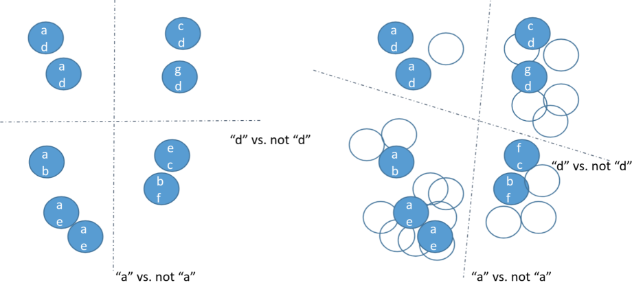
Figure 1: Semi-supervised learning in multi-label classification. Filled circles represent labeled examples, while empty circles represent unlabeled examples. Letters represent class labels.

In the literature, only a few existing approaches tackle the problem of semi-supervised multi-label classification and hierarchical multi-label classification. Examples include the work presented in [39, 23, 28] for the task of SSL MLC and the work presented in [38] for SSL HMLC. However, all these methods, adopt generative or optimization-based approaches, with the limitation that they result in complex and time-demanding learning processes which produce non-interpretable models. On the contrary, in this paper, we propose an approach to SSL MLC/HMLC which is based on predictive clustering trees (PCTs) [2]. The advantage is to learn in an efficient way an interpretable SSL MLC/HMLC prediction model.

The rest of the paper is structured as follows: in Section 2, we briefly describe the work in the literature that is related to the present paper; in Section 4, we describe the proposed solution, while, in Section 5, we evaluate its performance on publicly available datasets and discuss the results. Finally, in Section 7, we present the conclusions of the work and outline possible directions for future work.

2 Related Work and Motivations

SSL MLC is a relatively recent topic in machine learning and data mining. One of the most prominent works on this research topic is [23], where the main idea is to combine large-margin MLC with unsupervised subspace learning. This is done by jointly solving two problems: 1) learning a subspace representation of the labeled and unlabeled inputs and 2) learning a large-margin supervised multi-label classifier on the labeled part of the data. The proposed algorithm works in a single optimization step, which results in a high time complexity process. To alleviate the problem, the authors proposed a learning procedure which is based on subgradient search and coordinate descent.

In [28], the authors propose a SSL MLC algorithm based on the optimization problem of estimating label concept compositions (label co-occurrence). Specifically, the algorithm derives a closed-form solution to this optimization problem and then assigns label sets to the unlabeled instances in a transductive setting.

In [39] the authors propose a deep generative model to describe the label generation process for the SSL MLC task. For this purpose, the generative model incorporates latent variables to describe the labeled/unlabeled data as well as the labeling process. A sequential inference model is then used to approximate the model posterior and infer the ground truth labels. The same inference model is then used to predict the label of unlabeled instances.

All the mentioned works, although tackling the SSL MLC problem, suffer from the common problem of not generating interpretable models. This is not the case with the method proposed in this paper, where the adoption of the PCT framework allows us to produce multi-label decision trees, which are directly interpretable and fast to learn. Moreover, contrary to existing approaches, the approach we propose builds models by exploiting clustering. This allows us to properly take into account the smoothness assumption both for the descriptive space and for the output space. Finally, the mentioned existing approaches can not be directly used to impose limitations on the labels and, therefore, can not be directly used for the more complex task of HMLC.

As for the SSL HMLC task, the existing work in the literature is relatively limited. In [38] the authors extend the system RA$k$EL, originally developed for (supervised) MLC, to the SSL HMLC task, leading to three new methods, called HMC-SSBR, HMC-SSLP and HMC-SSRA$k$EL. RA$k$EL is an ensemble-based wrapper method for solving MLC tasks using existing algorithms for multi-class classification. They build the ensemble by providing a small random subset of $k$ labels (organized as a label powerset) to each base model, learned by a multi-class classifier. This approach is also used in HMC-SSBR, HMC-SSLP and HMC-SSRA$k$EL which, therefore, are not based on clustering and can not directly take into account the smoothness, the low-density, and the manifold assumptions.

In the more general context of semi-supervised structured output prediction, we can find some approaches for multi-target regression which also use predictive clustering trees. This is the case of the works in [30] and [31], where the idea is to learn predictive clustering trees by using both labeled and unlabeled examples. [30] proposed semi-supervised multi-target regression method based on the self-training approach with a random forest of predictive clustering trees. In self-training, a model is trained iteratively with its own most reliable predictions. [30] extended multi-target regression PCTs by adapting the heuristics used for the construction of the trees in order to consider both labeled and unlabeled examples. Both methods, however, do not tackle the classification task.

3 Background: Predictive clustering trees

The predictive clustering trees (PCTs) presented in this paper for MLC and HMLC, are inspired by the work in [2]. In that work, the splits in the tree are evaluated by considering both descriptive and target attributes. The semi-supervised decision trees proposed here have similarities to the ones in [2], with multiple differences. First, [2] considered unlabeled examples only in tasks with primitive outputs, whereas we designed semi-supervised trees for structured outputs. Second, we established a parameter that allows varying degrees of supervision in the trees (i.e., how much the descriptive attributes influence the evaluation of splits). With this we can build supervised, semi-supervised, or unsupervised trees, dictated by the demands of the specific dataset we are dealing with.

The PCT framework treats a decision tree as a hierarchically organized set of clusters, where the topmost cluster contains all data. This cluster is recursively divided into smaller clusters as one moves from the root to the leaves. They represent a generalization of default decision trees (e.g., C4.5 [36]) where the prediction targets more complex structures. Classical PCTs (i.e., unsupervised PCTs) can predict several types of structured outputs, including nominal/real value tuples [42, 26, 29], class hierarchies [45, 33, 32], and short time series [41]. For each type, two functions must be defined: the prototype function and the variance function. The prototype function associates a class label to each leaf in the tree, and it returns a representative structured value (i.e., a prototype) given a set of structured values. The variance function evaluates the homogeneity of a set of such structured values and is used to find the best splits in the nodes of the tree.

PCTs are learned with a top-down induction of decision trees (TDIDT) algorithm [5]. An input to the PCT algorithm (Algorithm 1) is a set of examples $E$. The heuristic ($h$) selects the best tests ($t^{*}$) on the basis of the reduction of variance resulting from partitioning ($\mathcal{P}$) the examples (BestTest function in Algorithm 1). As variance reduction is maximized, the homogeneity of the cluster is also maximized. If no suitable test is found, i.e., if none of the candidate tests results in a significant reduction of the variance or if there are fewer examples in a node than the specified limit, then a leaf is created and the prototype of the examples in that leaf is computed.

Table 1: Standard algorithm for PCT learning.

procedure PCT Input: A dataset $E$ Output: A predictive clustering tree 1:$(t^{*},h^{*},\mathcal{P}^{*})=\mathrm{BestTest}(E)$ 2:if $t^{*}\neq\mathit{none}$ then 3:    for each $E_{i}\in\mathcal{P^{*}}$ do 4:        $\mathit{tree}_{i}$ = PCT($E_{i}$)      5:    return $\mathrm{node}(t^{*},\;\bigcup_{i}\{\mathit{tree}_{i}\})$ 6:else 7:    return $\mathrm{leaf}(\mathrm{Prototype}(E))$

procedure $\mathrm{BestTest}$ Input: A dataset $E$ Output: the best test ($t^{*}$), its heuristic score ($h^{*}$) and the partition ($\mathcal{P}^{*}$) it induces on the dataset ($E$) 1:$(t^{*},h^{*},\mathcal{P}^{*})=(\mathit{none},0,\emptyset)$ 2:for each possible test $t$ do 3:    $\mathcal{P}=$ partition induced by $t$ on $E$ 4:    $h=\mathit{Var_{f}}(E)-\sum_{E_{i}\in\mathcal{P}}\frac{|E_{i}|}{|E|}\mathit{Var_{f}}(E_{i})$ 5:    if $(h>h^{*})\land\mathrm{Acceptable}(t,\mathcal{P})$ then 6:        $(t^{*},h^{*},\mathcal{P}^{*})=(t,h,\mathcal{P})$      7:return $(t^{*},h^{*},\mathcal{P}^{*})$

In this study, we propose semi-supervised PCTs, and ensembles of semi-supervised PCTs, for the tasks of MLC and HMLC. Thus, in Sections 3.1 and 3.2 we present supervised PCTs for these tasks in more detail.

To build an ensemble model for predicting a certain type of structured output, an appropriate type of PCTs is utilized as a base model. For example, to build an ensemble for the HMLC task, PCTs for HMLC are used as base models. An ensemble makes a prediction for a new example by taking into account predictions of all the ensemble’s base models. For regression tasks, predictions of the base models are averaged, while for classification tasks, various strategies can be used, such as the probability-based majority voting, which we used as suggested by [1]. In this strategy, each base tree gives the probability of an example belonging to each of the possible classes. The class that is predicted is the one with the highest sum of probabilities, considering all of the base trees.

3.1 PCTs for multi-label classification

The variance function for learning PCTs for the MLC task computes the average of the $Gini$ indices across all the target variables. For a set of examples $E$ with target space $Y$ consisting of $T$ nominal target variables $Y_{1},Y_{2},\ldots,Y_{T}$, the variance function is defined as follows:

$$Var_{f}(E,Y)=\frac{1}{T}\cdot\sum_{i=1}^{T}Gini(E,Y_{i}),$$ (1)

where $Gini(E,Y_{i})$ is the $Gini$ score of the $i^{th}$ target variable $Y_{i}$ for a set of examples $E$. The Gini score of the $i^{th}$ target variable is calculated as follows:

$$Gini(E,Y_{i})=1-\sum_{j=1}^{C_{i}}p_{j}^{2},$$ (2)

where $C_{i}$ is the number of classes for the target variable $Y_{i}$ (e.g., if $Y_{i}$ is binary, then $C_{i}=2$), and $p_{j}$ is the apriori empirical probability of a class $c_{j}$ (i.e., the relative frequency of instances in $E$ that belong to the class $c_{j}$).

The sum of the entropies of class variables can also be used as a variance indicator, i.e., $Var_{f}(E,Y)=\sum_{i=1}^{T}\mathit{Entropy(E,Y_{i})}$ (this was considered before for MLC [10]). The CLUS framework includes other variance functions as well, such as reduced error, gain ratio and the $m$-estimate.

The prototype function returns a vector denoting probabilities of an instance belonging to a given class for each target variable. To determine the predicted classes, the user can specify a threshold on probabilities, or the majority class (i.e., the most probable one) for each target can be calculated. In this study, we use the majority class.

3.2 PCTs for Hierarchical multi-label classification

In HMLC, the target space $Y$ is associated to a hierarchy of classes ($C,\leq_{h}$), where $\forall{c_{l},c_{j}\in C}:c_{l}\leq_{h}c_{j}\iff c_{l}\text{~{}is a superclass of~{}}c_{j}$. The set of labels of example $e_{i}$ is represented as a binary vector $L_{i}$, whose $j^{th}$ component is 1 if the example is labeled with the class $c_{j}$, 0 otherwise. The $j^{th}$ component of the arithmetic mean of such vectors contains the relative frequency of examples of the set belonging to class $c_{j}$. Now, the variance indicator over a set of examples $E$ is calculated as the average squared distance between each vector $(L_{i})$ and the set’s mean class vector $(\overline{L})$:

$$Var_{f}(E,Y)=\frac{1}{|E|}\cdot\sum\limits_{e_{i}\in E}d(L_{i},\overline{L})^{2}.$$ (3)

In the HMLC context, the similarities at higher levels of the hierarchy are considered as more important than the similarities at lower levels. The distance measure in the above formula (weighted Euclidean distance) is therefore defined as follows:

$$d(L_{1},L_{2})=\sqrt{\sum\limits_{l=1}^{|C|}\omega(c_{l})\cdot(L_{1,l}-L_{2,l}})^{2},$$ (4)

where $L_{i,l}$ is the $l^{th}$ component of the class vector $L_{i}$ of an instance $e_{i}$, $|C|$ is the number of classes in the hierarchy (i.e., the size of the class vector), and the class weights $\omega(c)$ decrease with the depth of the class in the hierarchy. More precisely, $\omega(c)=\omega_{0}^{depth(c)}$, where $depth(c)$ denotes the depth of the class $c$ in the hierarchy, and $0<w_{0}<1$. Note that, class weights can be calculated recursively, i.e., $\omega(c)=\omega_{0}\cdot\omega(par(c))$, where $par(c)$ denotes the parent of class $c$. In this work, we use $\omega_{0}=0.75$, as recommended by [45].

The definition of $\omega(c)$ is enough general to represent classes that are organized as a directed acyclic graph (DAG). Generally, a DAG-like hierarchy can be interpreted in two ways: an example belonging to a class $c$, either i) belongs to all super-classes of $c$, or ii) belongs to one or more superclasses of $c$. In this work, we consider the former situation.

The variance indicator for tree-structured hierarchies uses the weighted Euclidean distance between the class vectors (as defined in Equation 4), where the weight of a class changes depending on its level in the hierarchy. Note that, in DAG-shaped hierarchies, the classes do not have a unique level number. To resolve this issue, we adopt the recommendation of [45]: The weight of a given class is calculated as an average of all the weights according to possible paths from the root to that class.

In classification trees, a leaf holds the majority class of its examples which the tree predicts for examples arriving in that leaf. In the HMLC task, an example can have multiple classes, so it is not straightforward what the majority class means. The prediction, in this case, is a mean $\bar{L}$ of the class vectors of the examples in the leaf. The $i^{th}$ component of the vector $\bar{L}$ can be considered as the probability that an example in the leaf belongs to class $c_{i}$. The final classification for an example that arrived to the leaf can be done using a threshold $\tau$ to the probabilities; if $\bar{L_{i}}>\tau$ then class $c_{i}$ is predicted for the example. When making predictions, the parent-child relationships from the class hierarchy are preserved if the values for the thresholds $\tau$ are defined as follows: $\tau_{i}\leq\tau_{j}$ whenever $c_{i}\leq_{h}c_{j}$ ($c_{i}$ is ancestor of $c_{j}$). The selection of the threshold $\tau$ depends on the use scenario, e.g., trading off higher precision with lower recall. Here we use a metric that is not based on a threshold, but is based on precision-recall curves, so to take into account the predictive performance of the models.

4 Semi-supervised PCT learning for MLC and HMLC

4.1 Task definition

Here, we formally define the semi-supervised learning tasks for the types of structured outputs considered in this study: predicting multiple targets and hierarchical multi-label classification.

Semi-Supervised Multi-label classification

In MLC, the task is to predict several binary values (i.e., labels) for each example. More formally:

Given:

• A descriptive (or input) space $X=X_{1}\times X_{2}\times\ldots\times X_{D}$ spanned by $D$ descriptive variables that consist of values of primitive data types (boolean, nominal or continuous).

• A target (or output) space $Y=Y_{1}\times Y_{2}\times\ldots\times Y_{T}$ spanned by the $T$ binary target variables.

• A set of labeled examples $E_{l}=\left\{(x_{i},y_{i})\mid x_{i}\in X,y_{i}\in Y,1\leq i\leq N_{l}\right\}$, where each example $e_{i}\in E_{l}$ is described according to both the descriptive space and the target space, and $N_{l}$ is the number of labeled examples.

• A set of unlabeled examples $E_{u}=\left\{(x_{i})\mid x_{i}\in X,1\leq i\leq N_{u}\right\}$, where each example $e_{i}\in E_{u}$ takes values from the descriptive space only, and $N_{u}$ denotes the number of unlabeled examples.

• A quality metric $q$, e.g., which favors models with high predictive accuracy (or low predictive error).

Find: A function $f:X\rightarrow Y$ that maximizes $q$.

Semi-Supervised Hierarchical Multi-label classification

In HMLC, each example can have more than one class (multiple labels) and classes are organized in a hierarchical structure, i.e., an example belonging to a class also belongs to all its superclasses. More formally:

Given:

• A descriptive (or input) space $X=X_{1}\times X_{2}\times\ldots\times X_{D}$ spanned by $D$ descriptive variables that consist of values of primitive data types (boolean, nominal or continuous).

• A target space $Y$, defined with a hierarchy of classes ($C,\leq_{h}$), where $C$ is a set of classes and $\leq_{h}$ is a partial order among them, representing the superclass relationship, i.e., $\forall c_{1},c_{2}\in C,c_{1}\leq_{h}c_{2}$ if and only if $c_{1}$ is a superclass of $c_{2}$.

• A set of labeled examples $E_{l}=\left\{\left(x_{i},Y_{i}\right)\mid x_{i}\in X,Y_{i}\subseteq C,1\leq i\leq N_{l}\right\}$, where each example $e_{i}\in E_{l}$ is a pair of a tuple $x_{i}$ from the descriptive space and a set $S_{i}$ from the target space, and each set satisfies the hierarchy constraint, i.e., $c\in S_{i},c^{\prime}\in C,c^{\prime}\leq_{h}c\Rightarrow c^{\prime}\in Y_{i}$, and $N_{l}$ is the number of labeled examples.

• A set of unlabeled examples $E_{u}=\left\{(x_{i})\mid x_{i}\in X,1\leq i\leq N_{u}\right\}$, where each example $e_{i}\in E_{u}$ takes values from the descriptive space only, and $N_{u}$ is the number of unlabeled examples.

• A quality metric $q$, e.g., which favors models with high predictive accuracy (or low predictive error).

Find: a function $f:X\rightarrow 2^{C}$ (where $2^{C}$ is the power set of $C$) such that $f$ maximizes $q$ and the predictions made by $f$ satisfy the hierarchy constraint, i.e., $c\in f(x),c^{\prime}\in 2^{C},c^{\prime}\leq_{h}c\Rightarrow c^{\prime}\in f(x)$.

4.2 Tree learning

The proposed semi-supervised algorithm (SSL-PCTs) is based on the same tree induction algorithm as supervised PCTs, that is, the standard TDIDT algorithm (see Table 1).

The supervised TDIDT algorithm for PCTs is extended towards semi-supervised learning as follows. First, the input to the SSL algorithm dataset comprises both labeled and unlabeled examples: $E=E_{l}\cup E_{u}$, where $E_{l}$ are labeled examples and $E_{u}$ are unlabeled examples.

Second, the variance function in the SSL algorithm considers both the target and the descriptive attributes in the evaluation of splits. It is calculated as a weighted sum of the variance over the target space $Y$ and the variance over the descriptive space $X$:

$$Var_{f}(E,Y,X)=w\cdot Var_{f}(E,Y)+(1-w)\cdot Var_{f}(E,X),$$ (5)

where $w\in\left[0,1\right]$ is the parameter that controls the trade-off between the contribution of the target space and the descriptive space to the variance function.

This extension relies on the semi-supervised cluster assumption [8]: If examples are in the same cluster, then they are likely of the same class. Recall that, the variance function of supervised PCTs uses only the target attributes (Eq. 1 and 3). As a consequence, (a) unlabeled examples cannot contribute to the tree construction (since only their descriptive attributes are known), and (b) the clusters produced by supervised PCTs are only homogeneous regarding the class label. Enforcing the similarity of examples in both the descriptive and the target space during the construction of SSL-PCTs results in clusters that are homogeneous regarding both the descriptive and the target space and allows us to exploit both labeled and unlabeled examples. Finally, following the cluster assumption, labeled and unlabeled examples that end up in the same leaf of the tree are likely of the same class.

The $w$ parameter controls the magnitude of the contribution that unlabeled examples have on the learning of semi-supervised PCTs. In other words, the $w$ parameter enables learned models to range from fully supervised ($w=1$) to completely unsupervised ($w=0$). The control of the contribution of unlabeled examples by the $w$ parameter allows us to appropriately set the amount of supervision for different datasets. This aspect is discussed in more details in the experimental analysis (Section 6.3).

The variance of a set of examples $E$ on target space $Y$ is calculated differently depending on the type of structured output at hand:

$$Var_{f}(E,Y)=\begin{cases}\frac{1}{T}\cdot\sum_{i=1}^{T}Gini(E,Y_{i}),\text{ if }Y\text{ consists of }T\text{ binary variables}\\ \frac{1}{\sum\limits_{l=1}^{|C|}w(c_{l})}\left(\frac{1}{|E|}\cdot\sum\limits_{e_{i}\in E_{l}}d(L_{i},\overline{L})^{2}\right),\text{ if }Y\text{ is a hierarchy of classes}\end{cases}$$ (6)

Since the descriptive variables can be either numeric or nominal, the variance on the descriptive space of a set of examples $E$ is computed as follows:

$$Var_{f}(E,X)=\frac{1}{D}\cdot\left(\sum_{X_{i}\text{ is numeric}}Var(E,X_{i})+\sum_{X_{j}\text{ is nominal}}Gini(E,X_{j})\right),$$ (7)

where $D$ is the number of descriptive attributes and the variance or the Gini score of descriptive attributes is calculated following Eq. 8 and 9.

Let $N$ be the number of examples (both labeled and unlabeled), and let $K_{i}$ be the number of examples with non-missing values of the $i^{th}$ attribute $Y_{i}$. Now, variance for the continuous attributes and Gini index for the nominal attributes are calculated as follows, respectively:

$$Var(E,Y_{i})=\frac{\frac{N-1}{K_{i}-1}\cdot\sum_{j=1}^{K_{i}}(y_{i,j})^{2}-N\cdot\left(\frac{1}{K_{i}}\cdot\sum_{j=1}^{K_{i}}y_{i,j}\right)^{2}}{N},$$ (8)

$$Gini(E,Y_{i})=1-\sum_{j=1}^{C_{i}}{\left(\frac{\left|\{{e:e\in E\wedge c_{j}\in classes(e)\}}\right|}{K_{i}}\right)}^{2}=1-\sum_{j=1}^{C_{i}}\hat{p_{j}},$$ (9)

where $C_{i}$ is the number of class values of $Y_{i}$, and $\hat{p_{j}}$ is the apriori probability of class value $c_{j}$ estimated by using only examples for which the value for variable $Y_{i}$ is known. Note that for the HMLC task the variance for the output space is calculated only on the labeled data (see Eq. 6).

The variances (Gini indexes) of descriptive and target attributes are normalized, similarly to supervised PCTs, to ensure the equal contribution of attributes to the final variance. Normalization is performed by dividing the variance (Gini index) estimates of individual attributes in Eq. 8 (Eq. 9), considering the set of examples in the current node of the tree, with the variance (Gini index) of the corresponding attribute considering the entire training set.

During the semi-supervised tree construction phase, two extreme cases can occur: (1) Only unlabeled examples can end up in a leaf of the tree; therefore, the prototype function cannot be calculated. (2) Variance needs to be calculated for attributes where none of the examples (or only one) have non-missing values (e.g., $K_{i}\leq 1$ in Eq. 8). For the first extreme case, we calculate the prototype function of such a leaf by returning the prototype of the first parent node that contains labeled examples. Nodes with only unlabeled examples are not split further, while in leaf nodes containing labeled examples we allow minimum 2 labeled examples. Both criteria can be considered as “stopping criteria” to stop the tree construction phase. Note that, these criteria are coherent with the stopping criteria implemented in supervised PCTs, where at least two labeled examples in a leaf node are required.

The second extreme can occur when the examples in a node are split in a way that only unlabeled examples go into a single branch of the tree. In such case, a split needs to be evaluated with one of the branches containing only missing values for an attribute. This is handled by using the variance of the parent node instead. This solution is motivated by the fact that in this extreme case, coherently with the smoothness assumption, the only ”closer” information about labels we can assume is that of the containing “cluster”, that is the parent node.

4.2.1 Semi-supervised PCTs with Feature weighting

PCTs (and decision trees in general) are robust to irrelevant features since the learning algorithm chooses only the most informative features when building (supervised) trees. Thus, irrelevant features will be ignored. However, in semi-supervised PCTs this feature may be compromised since the evaluation of tests depends on target as well as descriptive attributes. To deal with this issue, we propose feature weighted SSL-PCTs.

Methods for feature weighting can be used to identify the most informative features among the irrelevant ones by determining an importance score (weight) corresponding to the information provided by a feature. A higher score denotes more informative features while a lower score denotes less informative ones. The effectiveness of feature weighting with the importance scores was shown to help the k-nearest neighbors algorithm to deal with irrelevant features [12]. Similarly, we adapt the SSL-PCTs and use importance scores to assign weights to features.

More specifically, we use a feature ranking method based on a random forest of PCTs [35] to obtain the importance score $\hat{\sigma_{i}}$ for each descriptive attribute $X_{i}$. To calculate feature importance, this method uses the internal out-of-bag (OOB) error as an estimate of the noise in the descriptive space. The rationale is that if noise is introduced to a descriptive variable which is important, then the error of the model will increase (as measured by OOB error estimates).

The feature ranking is performed on the labeled examples $E_{l}$ prior to building SSL-PCTs. The importance scores are then normalized as follows: $\sigma_{i}=\hat{\sigma_{i}}/\max(\hat{\sigma_{1}},\hat{\sigma_{2}},\ldots,\hat{\sigma_{D}})$. The function for calculation of variance of descriptive attributes of SSL-PCTs is then adapted to include normalized feature importance scores $\sigma_{i}$ as weights of the descriptive attribute $X_{i}$:

$$Var_{f}(E,X)=\frac{1}{D}\cdot\left(\sum_{X_{i}\text{ is numeric}}\sigma_{i}\cdot Var(E,X_{i})+\sum_{X_{j}\text{ is nominal}}\sigma_{j}\cdot Gini(E,X_{j})\right),$$ (10)

This results in irrelevant features contributing less to the variance score. Henceforth, semi-supervised PCTs with feature weighting are denoted as SSL-PCT-FR.

4.3 Semi-supervised random forests

SSL-PCTs can be easily extended to its random forest version [4]. This is done by using SSL-PCTs as the members of the random forest ensemble, instead of using classical supervised trees. The notable difference is, however, in the presence of both labeled and unlabeled examples in the bootstrap samples, which does not conform with the classical random forest algorithm [4]. In fact, the risk is that the trees are built using only a small set of labeled examples. In order to overcome this problem, in the semi-supervised setting, we perform stratified bootstrap sampling with respect to the proportions of labeled and unlabeled examples in order to avoid bootstrap samples being dominated by unlabeled examples (which in semi-supervised learning often greatly outnumber labeled examples).

4.4 Computational complexity

To asses the complexity of the algorithm for learning SSL-PCTs, we first introduce the computational complexity of learning supervised PCTs: sorting of $D$ descriptive variables ($\mathcal{O}(DN\log N)$), determining the best split for $T$ target variables ($\mathcal{O}(TDN)$), for $N$ labeled training examples ($O(N)$). If we assume that the expected depth of the tree is $\mathcal{O}(\log N)$ [47], the computational complexity of building a single PCT is $\mathcal{O}(DN\log^{2}N)+\mathcal{O}(TND\log N)+\mathcal{O}(N\log N)$.

Now we discuss the changes introduced in SSL-PCTs. These are, first, the number of training examples $N$ which in the semi-supervised case equals the combined number of unlabeled and labeled examples (i.e., $N=N_{l}+N_{u}$, instead of $N=N_{l}$). Second, SSL-PCTs use both $D$ descriptive variables and $T$ target variables to determine the best split, therefore, this step has the complexity of $\mathcal{O}((T+D)ND)$. Therefore, the computational complexity of building a SSL-PCT tree is $\mathcal{O}(DN\log^{2}N))+\mathcal{O}((D+T)ND\log N)+\mathcal{O}(N\log N)$.

The computational complexity of random forests of semi-supervised PCTs is bounded by $k(\mathcal{O}(D^{\prime}N^{\prime}\log^{2}N^{\prime})+\mathcal{O}((T+D)N^{\prime}D^{\prime}\log N^{\prime}))$, where $N^{\prime}$ is the number of the bootstrap samples, $D^{\prime}$ is the number of features considered at each tree node and $k$ is the number of trees. The added computational complexity of feature ranking is that of randomly permuting the values of the out-of-bag samples ($N^{\prime\prime}=N-N^{\prime}$) and sorting the samples through the tree. Both operations are done for each descriptive attribute and their cost is $O(DN^{\prime\prime}+D\log N)$. This added computational cost is, however, negligible compared to the overall cost of building the random forest ensemble. Note that, the number of examples in feature ranking is $E_{l}$ because the weights of features are calculated considering only the labeled examples.

5 Experimental design

In this section, we first describe the datasets used in the experimental evaluation. Next, we present the evaluation procedure, the specific parameter settings of the algorithms and, the performance measures.

5.1 Data description

To evaluate the proposed methods, we use 23 datasets of the two structured output prediction tasks considered: MLC and HMLC. The datasets are from various domains, and have different sizes and numbers of descriptive and target variables. The characteristics of the datasets are summarized in Tables 2 and 3 for the MLC and HMLC task, respectively.

Table 2: MLC datasets and their characteristics: $N$ is the number of examples, $D/C$ is the number of descriptive variables (nominal/continuous), $\mathcal{L}$ is the number of labels and $\overline{\mathcal{L}_{L}}$ is the average number of labels per example.

Dataset	Domain	$N$	$D/C$	$\mathcal{L}$	$\overline{\mathcal{L}_{L}}$
Bibtex [24]	Text	7395	1836/0	159	2.402
Birds [6]	Audio	645	2/258	19	1.014
Emotions [43]	Music	594	0/72	6	1.869
Corel5k [19]	Images	5000	499/0	374	3.522
Enron [25]	Text	1702	1001/0	53	3.378
Genbase [18]	Text	662	1186/0	27	1.252
Mediana [40]	Media	7953	21/58	5	1.205
Medical [37]	Text	978	1449/0	45	1.245
Scene [3]	Images	2407	0/294	6	1.074
SIGMEA real [13]	Ecology	817	0/4	2	0.726
Slovenian rivers [20]	Ecology	1060	0/16	14	5.073
Yeast [21]	Biology	2417	0/103	14	4.237

Table 3: HMLC datasets and their characteristics: $N$ is the number of examples, $D/C$ is the number of descriptive variables (nominal/continuous), $\mathcal{H}$ is the type of the label hierarchy, $|\mathcal{H}|$ is the number of nodes in the hierarchy, $\mathcal{H}_{d}$ is the maximal depth of the hierarchy, $\overline{\mathcal{L}_{L}}$ is the average number of labels per example.

Dataset	Domain	$N$	$D/C$	$\mathcal{H}$	$|\mathcal{H}|$	$\mathcal{H}_{d}$	$\overline{\mathcal{L}_{L}}$
Danish farms [14]	Ecology	1944	132/5	Tree	72	3	7
Diatoms [17]	Images	3119	0/371	Tree	377	3	0.94
Slovenian rivers [20]	Ecology	1060	0/16	Tree	724	4	25
ImCLEF07A [16]	Images	11006	0/80	Tree	96	3	1
ImCLEF07D [16]	Images	11006	0/80	Tree	46	3	1
Cellcycle-GO [45]	Genomics	3766	0/77	DAG	4126	12	35.91
Church-GO [45]	Genomics	3764	1/26	DAG	4126	12	35.89
Derisi-GO [45]	Genomics	3733	0/63	DAG	4120	12	35.99
Eisen-GO [45]	Genomics	2425	0/79	DAG	3574	11.12	39.04
Expr-GO [45]	Genomics	3788	4/547	DAG	4132	12	35.87
Pheno-GO [45]	Genomics	1592	69/0	DAG	3128	12	36.43

5.2 Experimental setup

We introduced semi-supervised PCTs (SSL-PCT) and their feature weighted variant (SSL-PCT-FR). We compare these methods across different structured output prediction tasks with supervised PCT algorithms for MLC and HMLC, denoted as SL-PCT in order to estimate the contribution of unlabeled data to the predictive performance of the methods under the same conditions. By such comparison, we can answer our main question: Are SSL-PCTs able to outperform supervised PCTs?. In the experiments with single trees, we use the pruning procedure as implemented in M5 regression trees [36].

We also compare the predictive performance of semi-supervised random forests (SSL-RF) and their feature weighted variant (SSL-RF-FR) to supervised random forests for structured output prediction (CLUS-RF). We use unpruned 100 trees to construct random forests. The number of randomly selected features at each node we set to $\left\lfloor{\log_{2}(D)+1}\right\rfloor$, where $D$ is the total number of features [4].

To assess the influence of different proportions of labeled/unlabeled data for the semi-supervised method, we vary the number of labeled examples across the following set of values: {50, 100, 200, 350, 500}. The labeled examples are randomly sampled from the training set, while the rest of the examples are used both as unlabeled examples and as testing data. We temporarily ignore their labels and use them in the semi-supervised methods as unlabeled training samples. The test set used to evaluate the models comprises the same examples and their original labels restored. The evaluation scenario is thus in the context of transductive learning. The supervised methods are trained using the selected labeled samples and evaluated on the same test set as semi-supervised methods. This is repeated 10 times using different random initialization, while the predictive performances are averaged over the 10 runs.

For each of the 10 runs, we optimize the parameter $w$ (weight) by an internal 3-fold cross-validation procedure performed on the labeled portion of the training set. The semi-supervised methods also use the available unlabeled examples. The values of the parameter $w$ vary from 0 to 1 with a step of 0.1.

The algorithms are evaluated by means of the area under the Precision-Recall curve (AUPRC). Since the considered tasks are MLC and HMLC, we use a variant of the AUPRC – the area under the micro-averaged average Precision-Recall curve ($\mathrm{AU}\overline{\mathrm{PRC}}$), as suggested by [45]. Specifically, the precision and recall values are computed as follows:

$$\overline{Prec}=\frac{\sum_{i}{TP}_{i}}{\sum_{i}{TP}_{i}+\sum_{i}{FP}_{i}},\quad\text{and}\quad\overline{Rec}=\frac{\sum_{i}{TP}_{i}}{\sum_{i}{TP}_{i}+\sum_{i}{FN}_{i}},$$

where $i$ ranges over all classes.

We statistically analyzed the results following the recommendations of [15]. We used the non-parametric Wilcoxon paired signed-rank test [46] for comparison of the predictive performance of two methods over multiple datasets. We set the significance level to 0.05 in all the experiments.

6 Results and discussion

6.1 Predictive performance of the methods

6.1.1 Multi-label classification

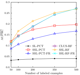
(a) Bibtex

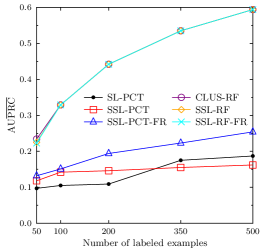
(b) Birds

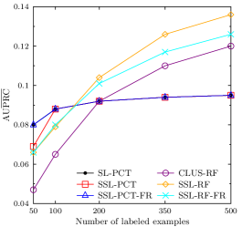
(c) Corel5k

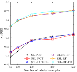
(d) Emotions

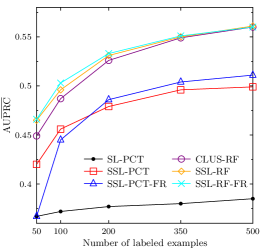
(e) Enron

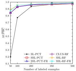
(f) Genbase

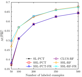
(g) Mediana

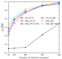
(h) Medical

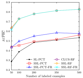
(i) Scene

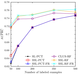
(j) SIGMEA real

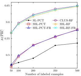
(k) Slovenian rivers

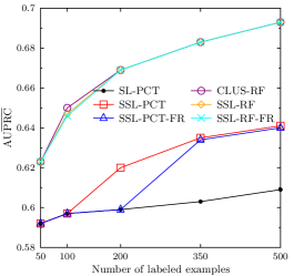
(l) Yeast

Figure 2: Predictive performance of the supervised and semi-supervised methods on the multi-label classification datasets.

Figure 2 presents the predictive performance ($\mathrm{AU}\overline{\mathrm{PRC}}$) of semi-supervised (SSL-PCT, SSL-PTC-FR, SSL-RF and SSL-RF-FR) and supervised methods (SL-PCT and CLUS-RF) on the 12 MLC datasets, with an increasing amount of labeled data.

We can clearly observe that semi-supervised PCTs are superior to SL-PCTs on most of the datasets. Namely, on 8 out of 12 datasets, either SSL-PCTs or SSL-PCT-FRs (or both) dominate the performance of SL-PCTs by a good margin. On the other four datasets, namely Corel5k, Emotions, Mediana and SIGMEA real, the performance of supervised and semi-supervised PCTs is mostly the same, or similar to the performance of SL-PCTs.

Intuitively, the improvement of semi-supervised over supervised methods should diminish as the number of labeled examples increases, and eventually semi-supervised and supervised methods are expected to converge to the same or similar performance. However, the “convergence point” changes from dataset to dataset. For instance, for Genbase, at 500 labeled examples we already see this convergence. For the other datasets, the improvement of semi-supervised over supervised methods does not decrease so fast.

The feature weighted semi-supervised method (SSL-PCT-FR) and the non feature weighted one (SSL-PCT) have similar trends in predictive performance. However, on some datasets, there are notable differences. Namely, on Birds and Scene datasets feature weighting is beneficial for the predictive performance of SSL-PCTs, and even necessary for improvement over SL-PCTs on the Birds dataset with $\geq$ 350 of labeled examples. On the other hand, feature weighting clearly hurts the predictive performance of the SSL-PCT method on the Bibtex dataset. Thus, feature weighting helps in most cases, but the empirical results cannot support its use by default when building SSL-PCTs for MLC.

We next compare semi-supervised random forests (SSL-RF) with supervised random forests (CLUS-RF). From the results, we can observe that CLUS-RF improves over CLUS-RF on several datasets: Bibtex, Corel5k, Genbase, Medical, SIGMEA real, and marginally on Emotions and Enron datasets. However, as compared to single trees, the improvements of the Semi-supervised approach over the supervised are observed on fewer datasets, and are smaller in MLC. In other terms, the improvement of SSL-PCTs over SL-PCTs does not guarantee the improvement of SSL-RF over CLUS-RF (e.g., Mediana, and Yeast datasets), and vice versa, SSL-RF can improve over CLUS-RF even if SSL-PCTs does not improve over SL-PCTs (e.g., SSL-RF-FR on Emotions dataset for 200 and 350 labeled examples). As observed for the single trees, there is no clear advantage of using feature weighting when semi-supervised random forests are built, even though it is somewhat on the Emotions and Enron datasets.

6.1.2 Hierarchical multi-label classification

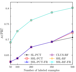
(a) Danish farms

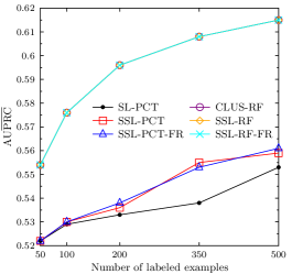
(b) Slovenian rivers

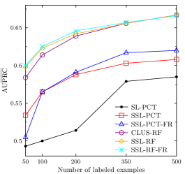
(c) Enron

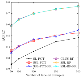
(d) ImCLEF07A

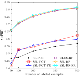
(e) ImCLEF07D

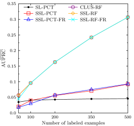
(f) Diatoms

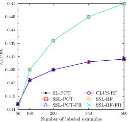
(g) Cellcycle-GO

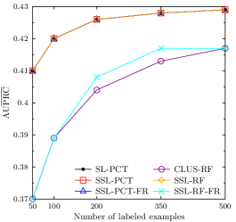
(h) Church-GO

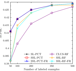
(i) Derisi-GO

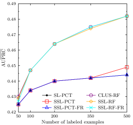
(j) Eisen-GO

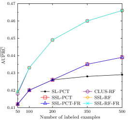
(k) Expr-GO

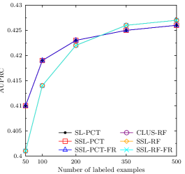
(l) Pheno-GO

Figure 3: Predictive performance of the supervised and semi-supervised methods on the hierarchical multi-label classification datasets.

Figure 3 presents the learning curves in terms of the predictive performance ($\mathrm{AU}\overline{\mathrm{PRC}}$) of semi-supervised (SSL-PCT, SSL-PTC-FR, SSL-RF and SSL-RF-FR) and supervised methods (SL-PCT and CLUS-RF) on the 11 hierarchical multi-label classification datasets.

We observe different behavior on the 6 functional genomics datasets and the 6 datasets from other domains. Namely, on all 6 datasets of the latter group, semi-supervised PCTs are improving over SL-PCTs – albeit not necessarily always for all available amounts of labeled data. This is the case on the Enron and ImCLEF07A datasets, where both SSL-PCTs and SSL-PCT-FR dominate the performance of SL-PCTs, while it seems that on other datasets at least 100 (Slovenian rivers and ImCLEF07D) or 500 (Danish farms) labeled examples are enough to improve over SL-PCTs.

On the other hand, semi-supervised PCTs are not so successful on functional genomics datasets. Analysis of the tree sizes (see Section 6.4) reveals an explanation for such results. Namely, on all of the 6 functional genomics datasets, and for almost all different amounts of labeled data, both supervised and semi-supervised trees are composed of only one node. Note that, these datasets have very large label hierarchies which are very sparsely populated. It seems that for such datasets the amount of labeled data we considered (i.e., up to 500 labeled examples) is not sufficient to build trees – either supervised or semi-supervised. In fact, semi-supervised trees have more than one node on Expr-GO ($\geq$350 of labeled examples) and Eisen (for 500 labeled examples) datasets, and those are exactly the occasions where they improve over supervised trees. We thus hypothesize that for larger amounts of labeled data, SSL-PCTs could outperform supervised PCT also on functional genomics datasets.

In the HMLC task, the feature weighted semi-supervised method (SSL-PCT-FR) and non-feature weighted one (SSL-PCT) mostly have very similar performance. Again, as for the MLC task, there is no clear benefit of feature weighting.

Finally, the semi-supervised random forests (SSL-RF and SSL-RF-FR) outperform supervised random forests (CLUS-RF) on some datasets, namely, in the initial part of the learning curve for the Enron dataset, and for the Church-GO and Derisi-GO datasets. On the other datasets, it seems that unlabeled data is not beneficial for the performance of random forests of PCTs for HMLC.

6.2 Statistical analysis of predictive performance

The results of the statistical analysis (Table 4) show that SSL-PCTs and SSL-PCT-FR are statistically significantly better than the SL-PCTs for most of the different amounts of labeled data considered for both structured output prediction tasks. More specifically, for the HMLC task, usually at least 200 labeled examples are needed to achieve statistical significance. On the MLC task, on the other hand, SSL-PCT achieves statistically significantly better results than SL-PCT up to 200 labeled examples. On this task, the feature weighted SSL-PCTs are more successful: They statistically significantly outperform SL-PCT across all different amounts of labeled examples.

Considering the feature-weighted and non-feature-weighted semi-supervised methods (both single trees and ensembles), in most cases, there is no statistically significant difference between them, except at the HMLC task for 200 labeled examples, where SSL-PCT-FR statistically significantly outperforms SSL-PCT.

As discussed previously, semi-supervised random forests improve over supervised ones in fewer cases as compared to single trees. A statistically significant improvement over CLUS-RF is observed only for the MLC task with 200 labeled examples and the HMLC task with 350 labeled examples. However, in none of the cases, the proposed semi-supervised methods perform statistically significantly worse than their supervised counterparts.

Table 4: P-values of the Wilcoxon signed-rank test applied to the predictive performances ($\mathrm{AU}\overline{\mathrm{PRC}}$) of the supervised and semi-supervised single trees (SL-PCT, SSL-PCT and SSL-PCT-FR) on the datasets considered in this study: 12 for multi-label classification and for 11 hierarchical multi-label classification. In bold, we report significant $p$-values ($<$ 0.05). In a comparison of the two algorithms, i.e., Algorithm1 vs. Algorithm2, the ’$-$’ sign indicates that the sum of ranks where the first algorithm outperformed the second is higher than the sum of ranks where the second algorithm outperformed the first. The ’$+$’ sign indicates the opposite.

Methods			Number of labeled examples
			50	100	200	350	500
Multi-label classification
SL-PCT	vs.	SSL-PCT	0.012 $(+)$	0.008 $(+)$	0.008 $(+)$	0.117 $(+)$	0.071 $(+)$
SL-PCT	vs.	SSL-PCT-FR	0.008 $(+)$	0.008 $(+)$	0.023 $(+)$	0.012 $(+)$	0.008 $(+)$
SSL-PCT	vs.	SSL-PCT-FR	0.969 $(+)$	0.666 $(+)$	0.556 $(+)$	0.078 $(+)$	0.182 $(+)$
CLUS-RF	vs.	SSL-RF	0.209 $(+)$	0.126 $(+)$	0.078 $(+)$	0.092 $(+)$	0.182 $(+)$
CLUS-RF	vs.	SSL-RF-FR	0.17 $(+)$	0.117 $(+)$	0.013 $(+)$	0.638 $(+)$	0.695 $(-)$
SSL-RF	vs.	SSL-RF-FR	0.937 $(+)$	0.209 $(+)$	0.754 $(-)$	0.327 $(-)$	0.388 $(-)$
Hierarchical multi-label classification
SL-PCT	vs.	SSL-PCT	0.937 $(+)$	0.147 $(+)$	0.034 $(+)$	0.025 $(+)$	0.008 $(+)$
SL-PCT	vs.	SSL-PCT-FR	1 $(-)$	0.158 $(+)$	0.034 $(+)$	0.025 $(+)$	0.01 $(+)$
SSL-PCT	vs.	SSL-PCT-FR	0.388 $(-)$	0.136 $(-)$	0.034 $(+)$	0.695 $(-)$	0.347 $(+)$
CLUS-RF	vs.	SSL-RF	0.367 $(+)$	0.136 $(+)$	0.099 $(+)$	0.347 $(+)$	0.136 $(+)$
CLUS-RF	vs.	SSL-RF-FR	1 $(-)$	0.347 $(+)$	0.136 $(+)$	0.034 $(+)$	0.48 $(+)$
SSL-RF	vs.	SSL-RF-FR	0.367 $(-)$	0.666 $(+)$	1 $(-)$	0.239 $(+)$	0.969 $(-)$

6.3 Influence of the amount of supervision

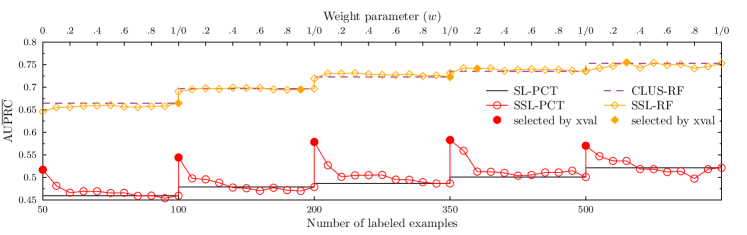
(a) Emotions (MLC)

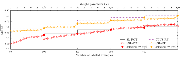
(b) Danish farms (HMLC)

Figure 4: Influence of the parameter $w$ on SSL-PCT (red line) and SSL-RF (orange line) methods. The results refer to 2 datasets with different types of structured outputs: Emotions (MLC) and Danish farms (HMLC). The $w$ values selected by the internal cross-validation algorithm and used in the experiments are marked with colored dots.

As mentioned before, the amount of supervision in the SSL-PCTs is controlled by the $w$ parameter, where $w=0$ results in unsupervised PCTs, $0<w<1$ in semi-supervised PCTs, and $w=1$ in supervised PCTs. Such ability to tune the degree of supervision in SSL-PCTs for the predictive problem at hand is of great practical importance. Namely, semi-supervised methods can, in general, degrade the performance of their supervised counterparts [34, 11, 48, 22]. In this respect, some studies noted that the success of semi-supervised methods is domain-dependent [9]. How to choose a suitable SSL method for the dataset at hand is an unresolved issue; therefore, even if the primary task of SSL methods is to improve the performance over supervised methods, making semi-supervised methods safe is also of high priority. In other words, we make sure that SSL methods do not degrade the performance of the corresponding supervised methods.

In SSL-PCTs, such a safety mechanism is provided by the $w$ parameter. Theoretically, given the optimal value of $w$, SSL-PCTs and SSL-RF would perform at least as well as their supervised counterparts both for MLC and HMLC. The reason is that SL-PCTs and CLUS-RF are a special cases of SSL-PCT and SSL-RF, respectively (they are the same if $w=1$). In practice, however, the $w$ parameter is chosen via internal cross-validation on labeled examples in the training set, thus it is possible to select $w$ sub-optimal for the test set considered.

Our empirical evaluation showed that, SSL-PCT and SSL-RF rarely degrade the performance of SL-PCT and CLUS-RF (Figures 2 and 3). Over all the experiments we performed, SSL-PCTs outperformed their supervised counterpart (SL-PCT) in 52% of experiments, performed worse on 9% of experiments, and equally on 39% of experiments. Moreover, the occasional degradation of the predictive performance was small compared to the improvements of SSL-PCT over SL-PCT. For example, the average relative improvement of SSL-PCTs over SL-PCTs (across all the experiments) is $40\%$, while the average degradation is $7\%$.

Figure 4 clearly shows the role of the parameter $w$ on the predictive performance for 2 datasets with different types of structured output. The Emotions dataset (Fig. 4a) requires no or small supervision because smaller $w$ give a better predictive performance of the SSL-PCT method. For the Danish farms dataset (Fig. 4b), on the other hand, more supervision (i.e., higher $w$) gives a better predictive performance of SSL-PCT. However, up to 500 labeled examples, the SSL-PCT method is unable to improve its supervised counterpart; therefore, $w=1$ is selected to prevent the performance degradation.

In conclusion, our results show that the optimal value of $w$ depends of the dataset and on the different amounts of labeled data, as exemplified in Figure 4. This confirms our initial intuition that different amount of supervision is suitable for different datasets. Therefore, it is difficult to provide a general recommendation for the value of $w$ and it is advisable to optimize this parameter by cross-validation for each dataset, as it is done in our study.

6.4 Interpretability of the models

Interpretability of the predictive models is often a desirable property of machine learning algorithms. Since the models produced by the SSL-PCTs are in the form of a decision tree, they are readily interpretable. To the best of our knowledge, in the literature, no other semi-supervised method for MLC and HMLC produces interpretable models.

The degree of interpretability of the tree-based models is typically expressed in terms of their size. A large tree can be difficult to interpret, and vice versa, a small tree can be easier to interpret. The tree size is sometimes considered a trade-off between accuracy and interpretability. Small trees are easy to interpret, but due to their simplicity may fail in capturing interactions in the data and therefore guarantee satisfactory accuracy. On the other hand, larger trees may mitigate such issues, but at the cost of lower interpretability. Note that increased size does not necessarily translate into the improved predictive power of tree models, due to possible overfitting problems. In general, it is not easy to identify (a priori) the best size of a tree, so to balance between overfitting and underfitting.

Table 5: Model sizes expressed as the number of nodes in trees, obtained with SL-PCTs SSL-PCTs on the 12 MLC datasets and 11 HMLC datasets.

Dataset	Number of labeled examples
	50		100		200		350		500
	SL	SSL	SL	SSL	SL	SSL	SL	SSL	SL	SSL
	-PCT	-PCT	-PCT	-PCT	-PCT	-PCT	-PCT	-PCT	-PCT	-PCT
Multi-label classification
Bibtex	1	21	1	21.4	1	19.4	1	19.4	1	19
Birds	1	15.8	1	20.8	1.2	15.2	2.6	13	4	12.8
Corel5k	1	33.6	1	1	1	1	1	1	1	1
Emotions	3	18.8	5	19	7.4	7.4	11.8	19.2	14.8	14.8
Enron	1	17.6	1	19.2	1	21.4	1	21.2	1.2	20.2
Genbase	2.6	22.8	21.4	23	31.2	26.6	37.2	36.8	43	41.4
Mediana	1.4	32.8	4	4	7.8	7.8	10.2	10.2	12.4	12.4
Medical	1	15.4	1	41.8	1	43.4	3.2	63.6	13.6	63.2
Scene	7.8	25.8	12.4	28.4	19.8	28.4	31.8	29	36.6	37.2
SIGMEA real	3	35.2	3.2	3.2	4.6	4.6	6.6	6.6	8.4	8.4
Slovenian rivers	1	39.2	1	64	1.4	67.6	3	70.8	3.8	55.8
Yeast	1	1	1	1	1	25	1.2	25	2.2	25
Average:	2.1	23.3	4.4	20.6	6.5	22.3	9.2	26.3	11.8	25.9
Hierarchical multi-label classification
Danish farms	1	1	1.4	1.4	3.2	3.2	6	6	8.8	257.6
Slovenian rivers	1	19.8	1	18.2	1	47.4	1.4	52.4	3	50.8
Enron	1	11.6	1	13.8	1.6	15.8	5.6	16.6	6.6	17.2
ImCLEF07A	1	42.8	2	86.6	6.6	133.4	12.8	150.4	19.4	177.4
ImCLEF07D	1	47.4	1.8	215	4.4	295.2	7	159.2	15	172.2
Diatoms	1	49.6	1	56.2	1	57.4	1	72.4	1	89.8
Cellcycle-GO	1	1	1	1	1	1	1	1	1	1
Church-GO	1	1	1	1	1	1	1	1	1	1
Derisi-GO	1	1	1	1	1	1	1	1	1	1
Eisen-GO	1	1	1	1	1	1	1	1	1	27.4
Expr-GO	1	1	1	1	1	1	1	9.2	1	9.2
Pheno-GO	1	1	1	1	1	1	1	1	1	1
Average:	1.0	14.9	1.2	33.1	2.0	46.5	3.3	39.3	5.0	67.1

In Table 5, we compare tree sizes of supervised and semi-supervised PCTs. We observe that, on average, the semi-supervised trees are somewhat larger than the supervised trees. This is intuitive since semi-supervised algorithms use much more data to grow the trees, i.e., both labeled and unlabeled examples. If we focus on individual datasets, we can observe that the size of both the supervised and semi-supervised trees is mainly in the range of a few tens of nodes. Which is still a reasonable size for manual inspection. However, there are few exceptions. Semi-supervised trees are sometimes, with a few hundreds of nodes, much larger than the corresponding supervised trees. In particular, this can be observed on the following datasets: Mediana ($\geq$ 350 labeled), Danish farms (500 labeled), ImCLEF07A, and ImCLEF07D ($\geq$ 200 labeled). These cases, generally characterized by a high number of classes, may be unfeasible for analysis.

A closer analysis of the results is shown in Figure 5, where it is possible to evaluate the influence of the $w$ parameter on the tree size. The analysis reveals that unsupervised trees ($w=0$) are much bigger in size than semi-supervised ($0<w<1$) or supervised ($w=1$) trees. Unsupervised trees do not rely on the output space at all, therefore, it is understandable that in the presence of a very large number of unlabeled data, big trees are grown. Recall that, the $w$ parameter was optimized for predictive performance, but by increasing the value of $w$ (i.e., increasing the degree of supervision) a trade-off between tree size and model performance can be achieved.

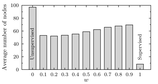
Figure 5: Average tree size per value of the $w$ parameter across all datasets and amounts of labeled data.

6.5 The influence of unlabeled data

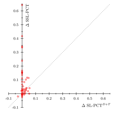
(a) Multi-label classification

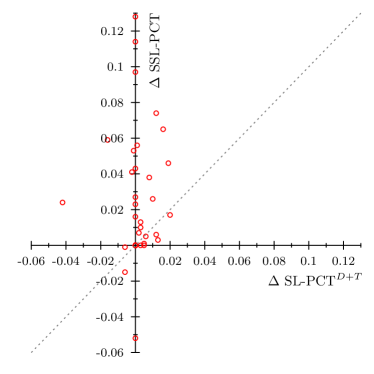
(b) Hierarchical multi-label classification

Figure 6: SSL-PCT and SL-PCT${}^{\text{D+T}}$ vs. SL-PCT considering all the datasets and different percentages of labeled data. $\Delta$SSL-PCT represents the difference between SL-PCT and SSL-PCT, while $\Delta$SL-PCT${}^{\text{D+T}}$ represents the difference between SL-PCT and SL-PCT${}^{\text{D+T}}$. SSL-PCT outperforms SL-PCT${}^{\text{D+T}}$ above the diagonal; SSL-PCT is better than SL-PCT for positive values on the $y$-axis; SSL-PCT is better than SL-PCT${}^{\text{D+T}}$ for positive values on the $x$-axis.

SSL-PCTs differ from supervised PCT mainly in two respects: i) they use both the descriptive attributes and target variables for the candidate split evaluation, and i) they use unlabeled examples in the training process. We have shown that SSL-PCTs have highly competitive predictive performance with respect to supervised PCTs, but we still can question the source of this improvement. Is this improvement motivated by the combination of i) and ii)? Or is i) enough to yield improvements over supervised PCTs? To answer to this question, we compared SSL-PCTs with the supervised modification of PCTs which exploits both the descriptive attributes and target variables for split evaluation but does not use unlabeled data (henceforth, this variant will be denoted as SL-PCT${}^{\text{D+T}}$). With such modification, we can properly evaluate the effect of the unlabeled examples to the predictive performance, since both SSL-PCTs and SL-PCT${}^{\text{D+T}}$ are trained using very similar algorithms with the only difference being in the usage of unlabeled data. In these experiments, we optimized the $w$ parameter for SL-PCT${}^{\text{D+T}}$ via internal 3-fold cross-validation, analogously to SSL-PCTs.

Considering all the datasets and the various percentages of labeled data, the SL-PCT${}^{\text{D+T}}$ algorithms perform better than the SL-PCT in 36% of cases, the same in 54% of cases and worse in 11% of cases. Recall that, the corresponding figures for the SSL-PCTs algorithm are 52%, 39% and 9%. Thus, even without the help of unlabeled data, the SSL-PCTs proposed in this work can improve over SL-PCTs, but they have a better chance to do so if they are supplied with unlabeled data. The following result provides evidence that the unlabeled data are indeed the principal component for the success of the SSL-PCT method: The average relative improvement of SL-PCT${}^{\text{D+T}}$ over SL-PCT is a mere 4%, while for SSL-PCT this figure is 40% (considering only the cases where SL-PCT${}^{\text{D+T}}$ and SSL-PCTs improve over SL-PCTs, respectively). This observation, i.e., the importance of unlabeled data, is in line with the findings of [49], where a rule learning process that considers both the descriptive and target spaces is adopted. The results reported in [49] show that the inclusion of the descriptive space into the heuristic was not beneficial for the predictive performance of predictive clustering rules. However, the study was performed in a supervised learning context, i.e., unlabeled examples were not used.

Finally, Figure 6 allows a detailed evaluation of improvement/degradation of SL-PCT${}^{\text{D+T}}$ over SL-PCT and of SL-PCT${}^{\text{D+T}}$ over SSL-PCT. As stated previously, the SSL-PCT method outperforms SL-PCT more often than SL-PCT${}^{\text{D+T}}$ (this happens when the points are above the diagonal). Furthermore, SSL-PCT yields much larger improvements over SL-PCT than SL-PCT${}^{\text{D+T}}$ (for most of the points on the figure, the improvement along the $y$-axis is much lager than the improvement along the $x$-axis). However, there is some complementarity between the two methods. Namely, SL-PCT${}^{\text{D+T}}$ sometimes improves over SL-PCT even when this is not the case with SSL-PCT (Figure 6, values on the positive side of the x-axis, below the dashed line).

7 Conclusions

In this study, we propose an algorithm for multi-label classification and for hierarchical multi-label classification that works in a semi-supervised learning setting. The method is based on predictive clustering trees and uses both the target and the descriptive space for the evaluation of candidate splits. The (empirically confirmed) intuition is that the usage of unlabeled examples allows the method to take advantage of the smoothness assumption of the semi-supervised learning setting, and therefore better exploit the label dependency introduced in MLC and in HMLC. Semi-supervised trees built in such a way can exploit unlabeled examples, while preserving the appealing characteristics of the supervised trees: producing readily interpretable models and being fast to learn.

In our experiments, we investigate whether the proposed semi-supervised predictive clustering trees and ensembles can outperform supervised predictive clustering trees and random forests. Next, we scrutinize various aspects of the proposed method: the influence of the amount of supervision via the $w$ parameter, model sizes and interpretability, and the influence of unlabeled data on the predictive performance of the algorithm. We performed the empirical evaluation over 12 datasets for the task of multi-label classification and 11 datasets for the task of hierarchical multi-label classification.

The proposed semi-supervised predictive clustering trees showed good predictive performance on both structured output tasks considered: On many of the datasets considered, their predictive performance was superior to that of supervised predictive clustering trees. Due to the parametrization which controls the amount of supervision, the proposed semi-supervised predictive clustering trees are safe to use: They do not degrade the performances with respect to their supervised analogs, they either outperform them or have the same performance. The degree of superiority of semi-supervised over supervised predictive clustering trees does not translate entirely to the tree ensembles, even though semi-supervised random forests often outperform supervised random forests. Other results showed that weighting descriptive attributes by their importance may help the predictive performance of semi-supervised predictive clustering in some cases, but the advantages are not strong enough to advocate the use of feature weighting by default. Thus, by the principle of Occam’s razor, the simpler solution should be preferred, that is, the one without feature weighting. Finally, the semi-supervised trees are marginally larger than the supervised trees, though the sizes of the trees are reasonable for manual inspection in most cases.

In future work, we intend to extend the proposed semi-supervised (hierarchical) multi-label classification algorithm to the case when examples are not independent and are accommodated in a network data structure. This would allow us to exploit the semi-supervised learning setting in network data, where the smoothness assumption naturally holds.

References

- [1] Bauer, E., and Kohavi, R. An empirical comparison of voting classification algorithms: Bagging, boosting, and variants. Machine Learning 36, 1 (1999), 105–139.
- [2] Blockeel, H., De Raedt, L., and Ramon, J. Top-down induction of clustering trees. In Proceeding of the 15th International Conference on Machine learning. Morgan Kaufmann, San Francisco, CA, 1998, pp. 55–63.
- [3] Boutell, M. R., Luo, J., Shen, X., and Brown, C. M. Learning multi-label scene classification. Pattern Recognition 37, 9 (2004), 1757–1771.
- [4] Breiman, L. Random forests. Machine Learning 45, 1 (2001), 5–32.
- [5] Breiman, L., Friedman, J., Olshen, R., and Stone, C. J. Classification and Regression Trees. Wadsworth & Brooks, Monterey, CA., 1984.
- [6] Briggs, F., Huang, Y., Raich, R., Eftaxias, K., Lei, Z., Cukierski, W., Hadley, S. F., Hadley, A., Betts, M., Fern, X. Z., Irvine, J., Neal, L., Thomas, A., Fodor, G., Tsoumakas, G., Ng, H. W., Nguyen, T. N. T., Huttunen, H., Ruusuvuori, P., Manninen, T., Diment, A., Virtanen, T., Marzat, J., Defretin, J., Callender, D., Hurlburt, C., Larrey, K., and Milakov, M. The 9th annual MLSP competition: New methods for acoustic classification of multiple simultaneous bird species in a noisy environment. In Proceedings of the IEEE International Workshop on Machine Learning for Signal Processing (2013), IEEE, pp. 1–8.
- [7] Ceci, M., Loglisci, C., Macchia, L., Malerba, D., and Quercia, L. Document image understanding through iterative transductive learning. In Digital Libraries and Archives - 8th Italian Research Conference, IRCDL 2012, Bari, Italy, February 9-10, 2012, Revised Selected Papers (2012), vol. 354 of Communications in Computer and Information Science, Springer, pp. 117–128.
- [8] Chapelle, O., Schölkopf, B., and Zien, A. Semi-supervised Learning. MIT Press, 2006.
- [9] Chawla, N., and Karakoulas, G. Learning from labeled and unlabeled data: An empirical study across techniques and domains. Journal of Artificial Intelligence Research 23, 1 (2005), 331–366.
- [10] Clare, A. Machine Learning and Data Mining for Yeast Functional Genomics. PhD thesis, University of Wales Aberystwyth, Aberystwyth, United Kingdom, 2003.
- [11] Cozman, F., Cohen, I., and Cirelo, M. Unlabeled data can degrade classification performance of generative classifiers. In Proceedings of the 15th International Florida Artificial Intelligence Research Society Conference (2002), AAAI, Palo Alto, California, pp. 327–331.
- [12] Cunningham, P., and Delany, S. J. k-nearest neighbour classifiers. Multiple Classifier Systems 34 (2007), 1–17.
- [13] Demšar, D., Debeljak, M., Lavigne, C., and Džeroski, S. Modelling pollen dispersal of genetically modified oilseed rape within the field. In Proceedings of the Annual Meeting of the Ecological Society of America (2005), p. 152.
- [14] Demšar, D., Džeroski, S., Larsen, T., Struyf, J., Axelsen, J., Pedersen, M., and Krogh, P. Using multi-objective classification to model communities of soil microarthopods. Ecological Modelling 191, 1 (2006), 131–143.
- [15] Demšar, J. Statistical comparisons of classifiers over multiple data sets. Journal of Machine Learning Research 7 (2006), 1–30.
- [16] Dimitrovski, I., Kocev, D., Loskovska, S., and Džeroski, S. Hierchical annotation of medical images. In Proceedings of the 11th International Multiconference Information Society (2008), Jožef Stefan Institute, Ljubljana, pp. 174–181.
- [17] Dimitrovski, I., Kocev, D., Loskovska, S., and Džeroski, S. Hierarchical classification of diatom images using ensembles of predictive clustering trees. Ecological Informatics 7, 1 (2012), 19–29.
- [18] Diplaris, S., Tsoumakas, G., Mitkas, P. A., and Vlahavas, I. Protein classification with multiple algorithms, vol. 3746 of Lecture Notes in Computer Science. Springer, Berlin, 2005, pp. 448–456.
- [19] Duygulu, P., Barnard, K., de Freitas, J. F. G., and Forsyth, D. A. Object Recognition as Machine Translation: Learning a Lexicon for a Fixed Image Vocabulary. Springer, Berlin, 2002, pp. 97–112.
- [20] Džeroski, S., Demšar, D., and Grbović, J. Predicting chemical parameters of river water quality from bioindicator data. Applied Intelligence 13, 1 (2000), 7–17.
- [21] Elisseeff, A., and Weston, J. A kernel method for multi-labelled classification. In Proccedings of the 15th Annual Conference on Neural Information Processing Systems (2001), MIT Press, Cambridge, Massachusetts, pp. 681–687.
- [22] Guo, Y., Niu, X., and Zhang, H. An extensive empirical study on semi-supervised learning. In Proceedings of the 10th IEEE International Conference on Data Mining (2010), IEEE, pp. 186–195.
- [23] Guo, Y., and Schuurmans, D. Semi-supervised multi-label classification - A simultaneous large-margin, subspace learning approach. In Machine Learning and Knowledge Discovery in Databases - European Conference, ECML PKDD 2012, Bristol, UK, September 24-28, 2012. Proceedings, Part II (2012), P. A. Flach, T. D. Bie, and N. Cristianini, Eds., vol. 7524 of Lecture Notes in Computer Science, Springer, pp. 355–370.
- [24] Katakis, I., Tsoumakas, G., and Vlahavas, I. Multilabel text classification for automated tag suggestion. In Proceedings of the ECML/PKDD 2008 Discovery Challenge (2008), vol. 75.
- [25] Klimt, B., and Yang, Y. The Enron Corpus: A New Dataset for Email Classification Research, vol. 3201 of Lecture Notes in Computer Science. Springer, Berlin, 2004, pp. 217–226.
- [26] Kocev, D., Vens, C., Struyf, J., and Džeroski, S. Ensembles of multi–objective decision trees. In Proceedings of the 18th European Conference on Machine Learning (2007), Springer, Berlin, pp. 624–631.
- [27] Kocev, D., Vens, C., Struyf, J., and Džeroski, S. Tree ensembles for predicting structured outputs. Pattern Recognition 46, 3 (2013), 817–833.
- [28] Kong, X., Ng, M. K., and Zhou, Z. Transductive multilabel learning via label set propagation. IEEE Trans. Knowl. Data Eng. 25, 3 (2013), 704–719.
- [29] Levatić, J., Ceci, M., Kocev, D., and Džeroski, S. Semi-supervised Learning for Multi-target Regression, vol. 8983 of Lecture Notes in Computer Science. Springer, Berlin, 2015, pp. 3–18.
- [30] Levatic, J., Ceci, M., Kocev, D., and Dzeroski, S. Self-training for multi-target regression with tree ensembles. Knowl. Based Syst. 123 (2017), 41–60.
- [31] Levatic, J., Kocev, D., Ceci, M., and Dzeroski, S. Semi-supervised trees for multi-target regression. Inf. Sci. 450 (2018), 109–127.
- [32] Levatić, J., Kocev, D., Debeljak, M., and Džeroski, S. Community structure models are improved by exploiting taxonomic rank with predictive clustering trees. Ecological Modelling 306 (2015), 294–304.
- [33] Levatić, J., Kocev, D., and Džeroski, S. The importance of the label hierarchy in hierarchical multi-label classification. Journal of Intelligent Information Systems 45, 2 (2014), 247–271.
- [34] Nigam, K., McCallum, A. K., Thrun, S., and Mitchell, T. Text classification from labeled and unlabeled documents using em. Machine learning 39, 2-3 (2000), 103–134.
- [35] Petković, M., Kocev, D., and Džeroski, S. Feature ranking for multi-target regression. Machine Learning Journal, 109 (2020), 1179––1204.
- [36] Quinlan, R. J. C4.5: Programs for Machine Learning, 1 ed. Morgan Kaufmann, 1993.
- [37] Read, J., Pfahringer, B., Holmes, G., and Frank, E. Classifier chains for multi-label classification. Machine Learning 85, 3 (2011), 333.
- [38] Santos, A. M., and Canuto, A. M. P. Applying semi-supervised learning in hierarchical multi-label classification. Expert Syst. Appl. 41, 14 (2014), 6075–6085.
- [39] Shi, W., Sheng, V. S., Li, X., and Gu, B. Semi-supervised multi-label learning from crowds via deep sequential generative model. In KDD ’20: The 26th ACM SIGKDD Conference on Knowledge Discovery and Data Mining, Virtual Event, CA, USA, August 23-27, 2020 (2020), R. Gupta, Y. Liu, J. Tang, and B. A. Prakash, Eds., ACM, pp. 1141–1149.
- [40] Skrjanc, M., Grobelnik, M., and Zupanic, D. Insights offered by data-mining when analyzing media space data. Informatica (Slovenia) 25, 3 (2001), 357–363.
- [41] Slavkov, I., Gjorgjioski, V., Struyf, J., and Džeroski, S. Finding explained groups of time-course gene expression profiles with predictive clustering trees. Molecular BioSystems 6, 4 (2010), 729–740.
- [42] Struyf, J., and Džeroski, S. Constraint Based Induction of Multi-objective Regression Trees, vol. 3933 of Lecture Notes in Computer Science. Springer, Berlin, 2006, pp. 222–233.
- [43] Trohidis, K., Tsoumakas, G., Kalliris, G., and Vlahavas, I. P. Multi-label classification of music into emotions. In Proceedings of the 9th International Conference on Music Information Retrieval (2008), vol. 8, Drexel University, Philadelphia, PA, pp. 325–330.
- [44] van Engelen, J. E., and Hoos, H. H. A survey on semi-supervised learning. Mach. Learn. 109, 2 (2020), 373–440.
- [45] Vens, C., Struyf, J., Schietgat, L., Džeroski, S., and Blockeel, H. Decision trees for hierarchical multi-label classification. Machine Learning 73, 2 (2008), 185–214.
- [46] Wilcoxon, F. Individual comparisons by ranking methods. Biometrics Bulletin 1 (1945), 80–83.
- [47] Witten, I. H., and Frank, E. Data Mining: Practical Machine Learning Tools and Techniques. Morgan Kaufmann, 2005.
- [48] Zhou, Z.-H., and Li, M. Semi-supervised regression with co-training style algorithms. IEEE Transaction on Knowledge and Data Engineering 19, 11 (2007), 1479–1493.
- [49] Ženko, B. Learning Predictive Clustering Rules. phdthesis, Faculty of Computer Science, University of Ljubljana, 2007.