Heterogeneous Treatment Effect with Trained Kernels of the Nadaraya-Watson Regression

Abstract

A new method for estimating the conditional average treatment effect is proposed in the paper. It is called TNW-CATE (the Trainable Nadaraya-Watson regression for CATE) and based on the assumption that the number of controls is rather large whereas the number of treatments is small. TNW-CATE uses the Nadaraya-Watson regression for predicting outcomes of patients from the control and treatment groups. The main idea behind TNW-CATE is to train kernels of the Nadaraya-Watson regression by using a weight sharing neural network of a specific form. The network is trained on controls, and it replaces standard kernels with a set of neural subnetworks with shared parameters such that every subnetwork implements the trainable kernel, but the whole network implements the Nadaraya-Watson estimator. The network memorizes how the feature vectors are located in the feature space. The proposed approach is similar to the transfer learning when domains of source and target data are similar, but tasks are different. Various numerical simulation experiments illustrate TNW-CATE and compare it with the well-known T-learner, S-learner and X-learner for several types of the control and treatment outcome functions. The code of proposed algorithms implementing TNW-CATE is available in https://github.com/Stasychbr/TNW-CATE.

Keywords: treatment effect, Nadaraya-Watson regression, neural network, shared weights, meta-learner, regression.

1 Introduction

The efficient treatment for a patient with her/his clinical and other characteristics [1, 2] can be regarded as an important goal of the real personalized medicine. The goal can be achieved by means of the machine learning methods due to the increasing amount of available electronic health records which are a basis for developing accurate models. To estimate the treatment effect, patients are divided into two groups called treatment and control, and then patients from the different groups are compared. One of the popular measures of the efficient treatment used in machine learning models is the average treatment effect (ATE) [3], which is estimated on the basis of observed data about patients as the mean difference between outcomes of patients from the treatment and control groups. Due to the difference between the patients characteristics and the difference between their responses to a particular treatment, the treatment effect is measured by the conditional average treatment effects (CATE) or the heterogeneous treatment effect (HTE) defined as ATE conditional on a patient feature vector [4, 5, 6, 7].

Two main problems can be pointed out when CATE is estimated. The first one is that the control group is usually larger than the treatment group. As a result, we meet the problem of a small training dataset, which does not allow us to apply directly many efficient machine learning methods. The second problem is that each patient cannot be simultaneously in the treatment and control groups, i.e., we either observe the patient outcome under treatment or control, but never both [8]. This is a fundamental problem of computing the causal effect. In addition to the above two problems, there are many difficulties of the machine learning model development concerning with noisy data, with the high dimension of the patient health records, etc. [9].

Many methods for estimating CATE have been proposed and developed due to importance of the problem in medicine and other applied areas [10, 11, 12, 13, 14, 15, 16, 17, 18, 19, 20, 21, 22, 23, 24]. This is only a small part of all publications which are devoted to solving the problem of estimating CATE. Various approaches were used for solving the problem, including the support vector machine [25], tree-based models [9], neural networks [26, 27, 8, 28], transformers [29, 30, 31, 32].

It should be noted that most approaches to estimating CATE are based on constructing regression models for handling the treatment and control groups. However, the problem of the small treatment group motivates to develop various tricks which at least partially resolve the problem.

We propose a method based on using the Nadaraya-Watson kernel regression [33, 34] which is widely applied to machine learning problems. The method is called TNW-CATE (the Trainable Nadaraya-Watson regression for CATE). The Nadaraya-Watson estimator can be seen as a weighted average of outcomes (patient responses) by means of a set of varying weights called attention weights. The attention weights in the Nadaraya-Watson regression are defined through kernels which measure distances between training feature vectors and the target feature vector, i.e., kernels in the Nadaraya-Watson regression conform with relevance of a training feature vector to a target feature vector. If we have a dataset $\{(\mathbf{x}_{1},y_{1}),...,(\mathbf{x}_{n},y_{n})\}$, where $\mathbf{x}_{i}\in\mathbb{R}^{m}$ is a feature vector (key) and $y_{i}\in\mathbb{R}$ is its target value or its label (value), then the Nadaraya-Watson estimator for a target feature vector $\mathbf{z}\in\mathbb{R}^{m}$ (query) can be defined by using weights $\alpha(\mathbf{z},\mathbf{x}_{i})$ as

$$\hat{f}(\mathbf{z})=\sum_{i=1}^{n}\alpha(\mathbf{z},\mathbf{x}_{i})y_{i},\ \alpha(\mathbf{z},\mathbf{x}_{i})=\frac{K(\mathbf{z},\mathbf{x}_{i},\gamma)}{\sum_{j=1}^{n}K(\mathbf{z},\mathbf{x}_{j},\gamma)},$$ (1)

where $K(\mathbf{z},\mathbf{x}_{i},\gamma)$ is a kernel and $\gamma>0$ is a bandwidth parameter.

Standard kernels widely used in practice are the Gaussian, uniform, or Epanechnikov kernels [35]. However, the choice of a kernel and its parameters significantly impact on results obtained from the Nadaraya-Watson regression usage. Moreover, the Nadaraya-Watson regression also requires a large number of training examples. Therefore, we propose a quite different way for implementing the Nadaraya-Watson regression. The way is based on the following assumptions and ideas. First, each kernel is represented as a part of a neural network implementing the Nadaraya-Watson regression. In other words, we do not use any predefined standard kernels like the Gaussian ones. Kernels are trained as the weight sharing neural subnetworks. The weight sharing is used to identically compute kernels under condition that pair $(\mathbf{z},\mathbf{x}_{i})$ of examples is fed into every subnetwork. The neural network kernels become more flexible and sensitive to a complex location structure of feature vectors. In fact, we propose to replace the definition of weights through kernels with a set of neural subnetworks with shared parameters (the neural network weights) such that every subnetwork implements the trainable kernel, but the whole network implements the Nadaraya-Watson estimator. At that, the trainable parameters of kernels are nothing else but weights of each neural subnetwork. The above implementation of the Nadaraya-Watson regression by means of the neural network leads to an interesting result when the treatment examples are considered as a single example whose “features” are the whole treatment feature vectors.

Second, it is assumed that the feature vector domains of the treatment and control groups are similar. For instance, if some components of the feature vectors from the control group are logarithmically located in the feature space, then the feature vectors from the treatment group have the same tendency to be located in the feature space. Fig. 1 illustrates the corresponding location of the feature vectors. Vectors from the control and treatment groups are depicted by small circles and triangles, respectively. It can be seen from Fig. 1 that the control examples as well as the treatment ones are located unevenly along the x-axis. Many standard regression methods do not take into account this peculiarity. Another illustration is shown in Fig. 2 where the feature vectors are located on spirals, but the spirals have different values of the patient outcomes. Even if we were to use a kernel regression, it is difficult to find such standard kernels that would satisfy training data. However, the assumption of similarity of domains allows us to train kernels on examples from the control group because kernels depend only on the feature vectors. In this case, the network memorizes how the feature vectors are located in the feature space. By using assumption about similarity of the treatment and control domains, we can apply the Nadaraya-Watson regression with the trained kernels to the treatment group changing the patient outcomes. TNW-CATE is similar to the transfer learning [36, 37, 38] when domains of source and target data are the same, but tasks are different. Therefore, the abbreviation TNW-CATE can be also read as the Transferable kernels of the Nadaraya-Watson regression for the CATE estimating.

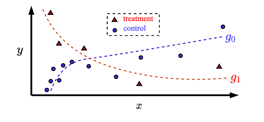
Figure 1: Illustration of the logarithmical location of feature vectors corresponding to patients from the treatment group (small triangles) and from the control group (small circles)

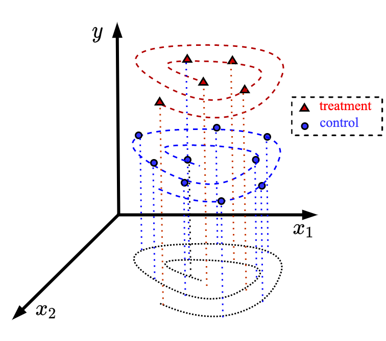
Figure 2: Illustration of the location of feature vectors corresponding to patients from the treatment group (small triangles) and from the control group (small circles) on spirals

Various numerical experiments study peculiarities of TNW-CATE and illustrate the outperformance of TNW-CATE in comparison with the well-known meta-models: the T-learner, the S-learner, the X-learner for several control and treatment output functions. The code of the proposed algorithms can be found in https://github.com/Stasychbr/TNW-CATE.

The paper is organized as follows. Section 2 can be viewed as a review of existing models for estimating CATE. Applications of the Nadaraya-Watson regression in machine learning also are considered in this section. A formal statement of the CATE estimation problem is provided in Section 3. TNW-CATE, its main ideas and algorithms implementing TNW-CATE are described in Section 4. Numerical experiments illustrating TNW-CATE and comparing it with other models are presented in Section 5. Concluding remarks are provided in Section 6.

2 Related work

Estimating CATE. Computing CATE is a very important problem which can be regarded as a tool for implementing the personalized medicine [39]. This fact motivated to develop many efficient approaches solving the problem. An approach based on the Lasso model for estimating CATE was proposed by Jeng et al. [40]. Several interesting approaches using the SVM model were presented in [25, 41]. A “honest” model for computing CATE was proposed by Athey and Imbens [12]. According to the model, the training set is splitting into two subsets such that the first one is used to construct the partition of the data into subpopulations that differ in the magnitude of their treatment effect, and the second subset is used to estimate treatment effects for each subpopulation. A unified framework for constructing fast tree-growing procedures solving the CATE problem was provided in [42, 43]. A modification of the survival causal tree method for estimating the CATE based on censored observational data was proposed in [44]. Xie et al. [45] established the CATE detection problem as a false positive rate control problem, and discussed in details the importance of this approach for solving large-scale CATE detection problems. Algorithms for estimating CATE in the context of Bayesian nonparametric inference were studied in [11]. Bayesian additive regression trees, causal forest, and causal boosting were compared under condition of binary outcomes in [9]. An orthogonal random forest as an algorithm that combines orthogonalization with generalized random forests for solving the CATE estimation problem was proposed in [46]. Estimating CATE as the anomaly detection problem was studied in [47]. Many other approaches can also be found in [48, 49, 50, 51, 52, 53, 54, 39, 55, 56, 57].

A set of meta-algorithms or meta-learners, including the T-learner [19], the S-learner [19], the O-learner [58], the X-learner [19] were investigated and compared in [19].

Neural networks can be regarded as one of the efficient tools for estimating CATE. As a result, many models based on using neural networks have been proposed [26, 59, 27, 60, 8, 61, 62, 63, 64, 65, 28, 66, 67].

Transformer-based architectures using attention operations [68] were also applied to solving the CATE estimating problem [29, 30, 31, 32]. Ideas of applying the transfer learning technique to the CATE estimation were considered in [69, 70, 71, 8]. Ideas of using the Nadaraya-Watson kernel regression in the CATE estimation were studied in [72, 73] where it was shown that the Nadaraya-Watson regression can be used for the CATE estimation. However, the small number of training examples in the treatment group does not allow us to efficiently apply this approach. Therefore, we aim to overcome this problem by introducing a neural network of a special architecture, which implements the trainable kernels in the Nadaraya-Watson regression.

The Nadaraya-Watson regression in machine learning. There are several machine learning approaches based on applying the Nadaraya-Watson regression [74, 75, 76, 77, 78, 79, 80]. Properties of the boosting with kernel regression estimates as weak learners were studied in [81]. A metric learning model with the Nadaraya-Watson kernel regression was proposed in [82]. The high-dimensional nonparametric regression models were considered in [83]. Models taking into account available correlated errors were proposed in [84]. An interesting work discussing a problem of embedding the Nadaraya-Watson regression into the neural network as a novel trainable CNN layer was presented in [85]. Applied machine learning problems solved by using the Nadaraya-Watson regression were considered in [86]. A method of approximation using the kernel functions made from only the sample points in the neighborhood of input values to simplify the Nadaraya-Watson estimator is proposed in [87]. An interesting application of the Nadaraya-Watson regression to improving the local explanation method SHAP is presented in [88] where authors find that the Nadaraya-Watson estimator can be expressed as a self-normalized importance sampling estimator. An explanation of how the Nadaraya-Watson regression can be regarded as a basis for understanding the attention mechanism from the statistics point of view can be found in [68, 89].

In contrast to the above works, we pursue two goals. The first one is to show how kernels in the Nadaraya-Watson regression can be implemented and trained as neural networks of a special form. The second goal is to apply the whole neural network implementing the Nadaraya-Watson regression to the problem of estimating CATE.

3 A formal problem statement

Suppose that the control group of patients is represented as a set of $c$ examples of the form $\mathcal{C}=\{(\mathbf{x}_{1},y_{1}),...,(\mathbf{x}_{c},y_{c})\}$, where $\mathbf{x}_{i}=(x_{i1},...,x_{id})\in\mathbb{R}^{d}$ is the $d$-dimensional feature vector for the $i$-th patient from the control group; $y_{i}\in\mathbb{R}$ is the $i$-th observed outcome, for example, time to death of the $i$-th patient from the control group or the blood sugar level of this patient. The similar notations can be introduced for the treatment group containing $t$ patients, namely, $\mathcal{T}=\{(\mathbf{z}_{1},h_{1}),...,(\mathbf{z}_{t},h_{t})\}$. Here $\mathbf{z}_{i}=(z_{i1},...,z_{id})\in\mathbb{R}^{d}$ and $h_{i}\in\mathbb{R}$ are the feature vector and the outcome of the $i$-th patient from the treatment group, respectively. We will also use the notation of the treatment assignment indicator $T_{i}\in\{0,1\}$ where $T_{i}=0$ ($T_{i}=1$) corresponds to the control (treatment) group.

Let $Y$ and $H$ denote the potential outcomes of a patient if he had received treatment $T=0$ and $T=1$, respectively. Let $\mathbf{X}$ be the random feature vector from $\mathbb{R}^{d}$. The treatment effect for a new patient with the feature vector $\mathbf{x}$, which shows how the treatment is useful and efficient, is estimated by the Individual Treatment Effect (ITE) defined as $H-Y$. Since the ITE cannot be observed, then the treatment effect is estimated by means of CATE which is defined as the expected difference between two potential outcomes as follows [90]:

$$\tau(\mathbf{x})=\mathbb{E}\left[H-Y|\mathbf{X}=\mathbf{x}\right].$$ (2)

The fundamental problem of computing CATE is that, for each patient in the training dataset, we can observe only one of outcomes $y$ or $h$ for each patient. To overcome this problem, the important assumption of unconfoundedness [91] is used to allow the untreated units to be used to construct an unbiased counterfactual for the treatment group [92]. According to the assumption of unconfoundedness, the treatment assignment $T$ is independent of the potential outcomes for $Y$ or H conditional on $\mathbf{x}=\mathbf{z}$, respectively, which can be written as

$$T\perp\{Y,H\}|\mathbf{x}.$$ (3)

Another assumption called the overlap assumption regards the joint distribution of treatments and covariates. According to the assumption, there is a positive probability of being both treated and untreated for each value of $\mathbf{x}$. It is of the form:

$$0<\Pr\{T=1|\mathbf{x}\}<1.$$ (4)

If to accept these assumptions, then CATE can be represented as follows:

$$\tau(\mathbf{x})=\mathbb{E}\left[H|\mathbf{X}=\mathbf{x}\right]-\mathbb{E}\left[Y|\mathbf{X}=\mathbf{z}\right].$$ (5)

The motivation behind unconfoundedness is that nearby observations in the feature space can be treated as having come from a randomized experiment [93].

If we suppose that outcomes of patients from the control and treatment groups are expressed through the functions $g_{0}$ and $g_{1}$ of the feature vectors $X$, then the corresponding regression functions can be written as

$$y=g_{0}(\mathbf{x})+\varepsilon,\ \mathbf{x}\in\mathcal{C},$$ (6)

$$h=g_{1}(\mathbf{z})+\varepsilon,\ \mathbf{z}\in\mathcal{T}.$$ (7)

Here $\varepsilon$ is a is a Gaussian noise variable such that $\mathbb{E}(\varepsilon)=0$. Hence, there holds under condition $\mathbf{x}=\mathbf{z}$

$$\tau(\mathbf{x})=g_{1}(\mathbf{x})-g_{0}(\mathbf{x}).$$ (8)

An example illustrating sets of controls (small circles), treatments (small triangles) and the corresponding unknown function $g_{0}$ and $g_{1}$ are shown Fig. 1.

4 The TNW-CATE description

It has been mentioned that the main idea behind TNW-CATE is to replace the Nadaraya-Watson regression with the neural network of a specific form. The whole network consists of two main parts. The first part implements the Nadaraya-Watson regression for training the control function $g_{0}(\mathbf{x})$. In turn, it consists of $n$ identical subnetworks such that each subnetwork implements the attention weight $\alpha(\mathbf{x},\mathbf{x}_{i})$ or the kernel $K(\mathbf{x},\mathbf{x}_{i})$ of the Nadaraya-Watson regression. Therefore, the input of each subnetwork is two vectors $\mathbf{x}$ and $\mathbf{x}_{i}$, i.e., two vectors $\mathbf{x}$ and $\mathbf{x}_{i}$ are fed to each subnetwork. The whole network consisting of $n$ identical subnetworks and implementing the Nadaraya-Watson regression for training the control function will be called the control network. In order to train the control network, for every vector $\mathbf{x}_{i}$, $i=1,...,c$, $N$ subsets of size $n$ are randomly selected from the control set $\mathcal{C}$ without example $(\mathbf{x}_{i},y_{i})$. The subsets can be regarded as $N$ examples for training the network. Hence, the control network is trained on $N\cdot c$ examples of size $2d\cdot n$. If we have a feature vector $\mathbf{x}$ for estimating $\tilde{y},$ i.e., for estimating function $g_{0}(\mathbf{x})$, then it is fed to each trained subnetworks jointly with each $\mathbf{x}_{i}$, $i=1,...,c$, from the training set. In this case, the trained weights or kernels of the Nadaraya-Watson regression are used to estimate $\tilde{y}$. The number of subnetworks for testing is equal to the number of training examples $n$ in every subset. Since the trained subnetworks are identical and have the same weights (parameters), then their number can be arbitrary. In fact, a single subnetwork can be used in practice, but its output depends on the pair of vectors $\mathbf{x}$ and $\mathbf{x}_{i}$.

Quite the same network called the treatment network is constructed for the treatment group. In contrast to the control network, it consists of $m$ subnetworks with inputs in the form of pairs $(\mathbf{z},\mathbf{z}_{i})$. In the same way, $M$ subsets of size $m$ are randomly selected from the training set of treatments without the example $(\mathbf{z}_{j},h_{j})$, $j=1,...,t$. The treatment network is trained on $M\cdot t$ examples of size $2d\cdot m$. After training, the treatment network allows us to estimate $\tilde{h}$ as function $g_{1}(\mathbf{z})$. If $\mathbf{z}=\mathbf{x}$, then we get an estimate of CATE $\tau(\mathbf{x})$ or $\tau(\mathbf{z})$ as the difference between estimates $\tilde{h}$ and $\tilde{y}$ obtained by using the treatment and control neural networks. It is important to point out that the control and treatment networks are jointly trained by using the loss function defined below.

Let us formally describe TNW-CATE in detail. Consider the control group of patients $\mathcal{C}=\{(\mathbf{x}_{1},y_{1}),...,(\mathbf{x}_{c},y_{c})\}$. For every $i$ from set $\{1,...,c\}$, we define $N$ subsets $\mathcal{C}_{i,r}$, $r=1,...,N$, consisting of $n$ examples randomly selected from $\mathcal{C}\backslash(\mathbf{x}_{i},y_{i})$ as:

$$\mathcal{C}_{i,r}=\{(\mathbf{x}_{1}^{(r)},y_{1}^{(r)}),...,(\mathbf{x}_{n}^{(r)},y_{n}^{(r)})\},\ r=1,...,N,$$ (9)

where $\mathbf{x}_{j}^{(r)}$ is a randomly selected vector of features from the set $\{\mathbf{x}_{1},...,\mathbf{x}_{c}\}\backslash\mathbf{x}_{i}$, which forms $\mathcal{C}_{i,r}$; $y_{j}^{(r)}$ is the corresponding outcome.

Each subsets $\mathcal{C}_{i,r}$ jointly with $(\mathbf{x}_{i},y_{i})$ forms a training example for the control network as follows:

$$\mathbf{a}_{i}^{(r)}=\left(\mathbf{x}_{1}^{(r)},...,\mathbf{x}_{n}^{(r)},\mathbf{x}_{i},y_{1}^{(r)},...,y_{n}^{(r)},y_{i}\right),\ i=1,...,c,\ r=1,...,N.$$ (10)

If we feed this example to the control network, then we expect to get some approximation $\tilde{y}_{i}^{(r)}$ of $y_{i}$. The number of the above examples for training is $N\cdot c$.

Let us consider the treatment group of patients $\mathcal{T}=\{(\mathbf{z}_{1},h_{1}),...,(\mathbf{z}_{t},h_{t})\}$ now. For every $j$ from set $\{1,...,t\}$, we define $M$ subsets $\mathcal{T}_{j,s}$, $s=1,...,M$, consisting of $m$ examples randomly selected from $\mathcal{T}\backslash(\mathbf{z}_{j},h_{j})$ as:

$$\mathcal{T}_{j,s}=\{(\mathbf{z}_{1}^{(s)},h_{1}^{(s)}),...,(\mathbf{z}_{m}^{(s)},h_{m}^{(s)})\},\ s=1,...,M,$$ (11)

where $\mathbf{z}_{l}^{(s)}$ is a randomly selected vector of features from the set $\{\mathbf{z}_{1},...,\mathbf{z}_{t}\}\backslash\mathbf{z}_{j}$, which forms $\mathcal{T}_{j,s}$; $h_{j}^{(s)}$ is the corresponding outcome.

Each subsets $\mathcal{T}_{j,s}$ jointly with $(\mathbf{z}_{j},h_{j})$ forms a training example for the control network as follows:

$$\mathbf{b}_{j}^{(s)}=\left(\mathbf{z}_{1}^{(s)},...,\mathbf{z}_{m}^{(s)},\mathbf{z}_{j},h_{1}^{(s)},...,h_{m}^{(s)},h_{j}\right),\ j=1,...,t,\ s=1,...,M.$$ (12)

If we feed this example to the treatment network, then we expect to get some approximation $\tilde{h}_{j}^{(s)}$ of $h_{j}$. Indices $r$ and $s$ are used to distinguish subsets of controls and treatments.

The architecture of the joint neural network consisting of the control and treatment networks is shown in Fig. 3. One can see from Fig. 3 that normalized outputs $\alpha_{i,j}^{(r)}$ and $\delta_{j,l}^{(s)}$ of the subnetworks in the control and treatment networks are multiplied by $y_{j}^{(r)}$ and $h_{l}^{(s)}$, respectively, and then the obtained results are summed. Here $\alpha_{i,1}^{(r)}+...+\alpha_{i,n}^{(r)}=1$ and $\delta_{j,1}^{(s)}+...+\delta_{j,m}^{(s)}=1$. It should be noted again that the control and treatment networks have the same parameters (weights). Every network implements the Nadaraya-Watson regression with this architecture, i.e.,

$$\tilde{y}_{i}^{(r)}=g_{0}(\mathbf{x}_{i})=\sum_{j=1}^{n}\alpha_{i,j}^{(r)}y_{j}^{(k)},\ \tilde{h}_{j}^{(s)}=g_{1}(\mathbf{z}_{j})=\sum_{j=1}^{n}\delta_{i,j}^{(s)}h_{j}^{(s)},$$ (13)

Here

$$\alpha_{i,j}^{(r)}=\alpha(\mathbf{x}_{i},\mathbf{x}_{j}^{(r)})=\frac{K\left(\mathbf{x}_{i},\mathbf{x}_{j}^{(r)}\right)}{\sum_{k=1}^{n}K\left(\mathbf{x}_{i},\mathbf{x}_{k}^{(r)}\right)},$$ (14)

$$\delta_{i,j}^{(s)}=\delta(\mathbf{z}_{j},\mathbf{z}_{i}^{(s)})=\frac{K\left(\mathbf{z}_{j},\mathbf{z}_{i}^{(s)}\right)}{\sum_{k=1}^{m}K\left(\mathbf{z}_{j},\mathbf{z}_{k}^{(s)}\right)}.$$ (15)

If to consider the whole neural network, then training examples are of the form:

$$\left(\mathbf{a}_{i}^{(r)},\mathbf{b}_{j}^{(s)}\right),\ i=1,...,c,\ j=1,...,t,~{}r=1,...,N,\ s=1,...,M.$$ (16)

The standard expected $L_{2}$ loss function for training the whole network is of the form:

$$L =\frac{1}{N\cdot c}\sum_{r=1}^{N}\sum_{i=1}^{c}\left(\tilde{y}_{i}^{(r)}-y_{i}\right)^{2}+\alpha\frac{1}{M\cdot t}\sum_{s=1}^{M}\sum_{j=1}^{t}\left(\tilde{h}_{j}^{(s)}-h_{j}\right)^{2}$$

$$=\frac{1}{N\cdot c}\sum_{r=1}^{N}\sum_{i=1}^{c}\left(g_{0}\left(\mathbf{a}_{i}^{(r)}\right)-y_{i}\right)^{2}+\alpha\frac{1}{M\cdot t}\sum_{s=1}^{M}\sum_{j=1}^{t}\left(g_{1}\left(\mathbf{b}_{j}^{(s)}\right)-h_{j}\right)^{2}.$$ (17)

Here $\alpha$ is the coefficient which controls how the treatment networks impacts on the training process. In particular, if $\alpha=0$, then only the control network is trained on controls without treatments.

In sum, we achieve our first goal to train subnetworks implementing kernels in the Nadaraya-Watson regression by using examples from control and treatment groups. The trained kernels take into account structures of the treatment and control data. The next task is to estimate CATE by using the trained kernels for some new vectors $\mathbf{x}$ or $\mathbf{z}$. It should be noted that all subnetworks can be represented as a single network due to shared weights. In this case, arbitrary batches of pairs $(\mathbf{x},\mathbf{x}_{i})$ and pairs $(\mathbf{z},\mathbf{z}_{j})$ can be fed to the single network. This implies that we can construct testing neural networks consisting of $c$ and $t$ trained subnetworks in order to estimate $\tilde{y}$ and $\tilde{h}$ corresponding to $\mathbf{z}$ and $\mathbf{x}$, respectively, under condition $\mathbf{z}=\mathbf{x}$. Figs. 4 and 5 show trained neural networks for estimating $\tilde{y}$ and $\tilde{h}$, respectively. It is important to point out that the testing networks are not trained. Sets of $c$ pairs $(\mathbf{x},\mathbf{x}_{1}),...,(\mathbf{x},\mathbf{x}_{c})$ and $t$ pairs $(\mathbf{z},\mathbf{z}_{1}),...,(\mathbf{z},\mathbf{z}_{t})$ are fed to the subnetworks of the control and treatment networks, respectively. The whole examples for testing taking into account outcomes are

$$\mathbf{a}(\mathbf{x})=\left(\mathbf{x}_{1},...,\mathbf{x}_{c},\mathbf{x},y_{1},...,y_{c}\right),$$ (18)

and

$$\mathbf{b}(\mathbf{z})=\left(\mathbf{z}_{1},...,\mathbf{z}_{c},\mathbf{z},h_{1},...,h_{t}\right).$$ (19)

In sum, the networks implement the Nadaraya-Watson regressions:

$$\tilde{y}=g_{0}(\mathbf{x})=\sum_{j=1}^{c}\alpha(\mathbf{x},\mathbf{x}_{j})y_{j},\ \tilde{h}=g_{1}(\mathbf{z})=\sum_{i=1}^{t}\delta(\mathbf{z},\mathbf{z}_{i})h_{i}.$$ (20)

Finally, CATE $\tau(\mathbf{x})$ or $\tau(\mathbf{z})$ is estimated as $\tau(\mathbf{x})=\tau(\mathbf{z})=\tilde{h}-\tilde{y}$.

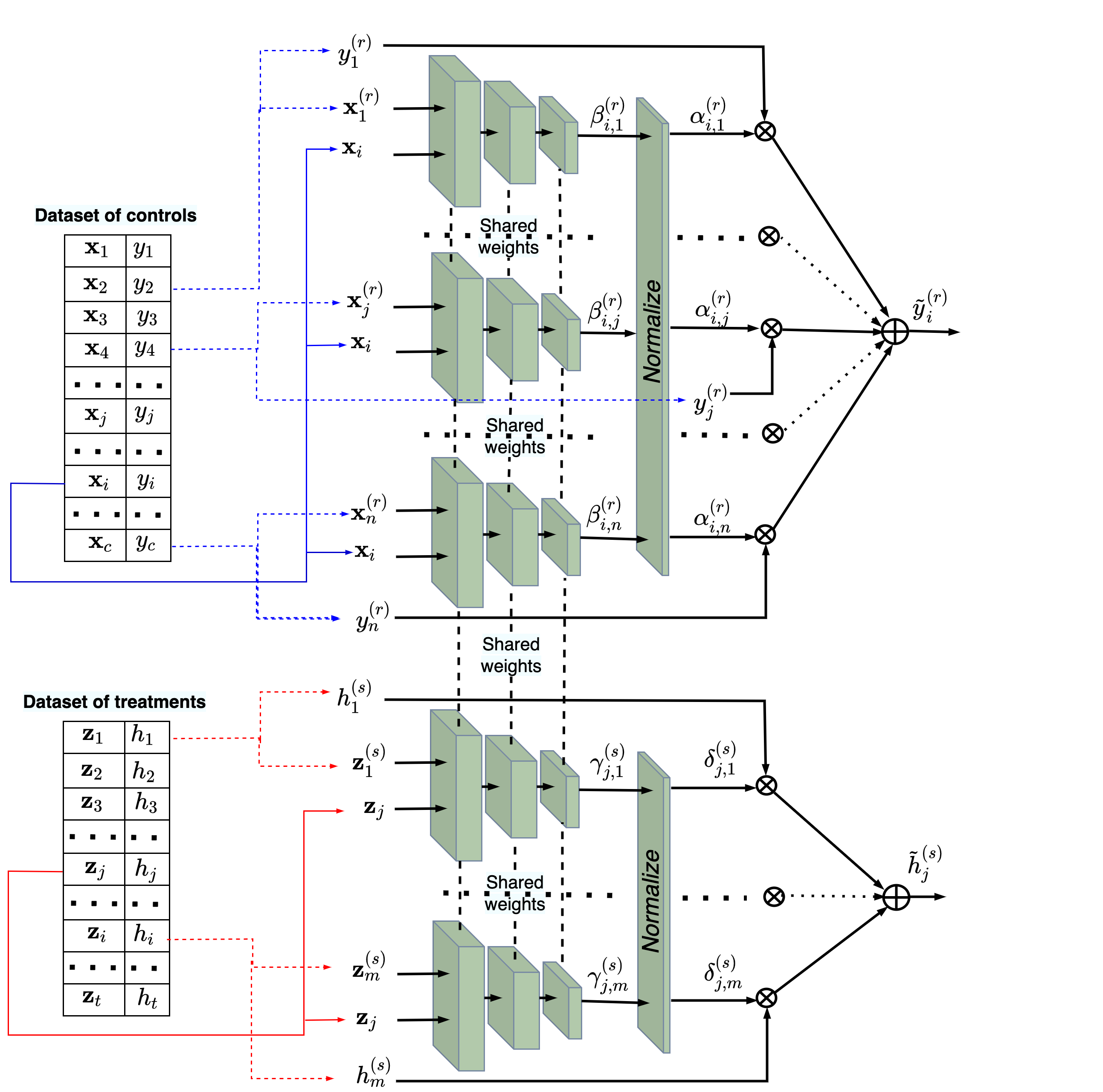
Figure 3: The weight sharing neural network consisting of $n$ subnetworks for training on controls and $m$ subnetworks for training on treatments, which implements two models of the Nadaraya-Watson regression

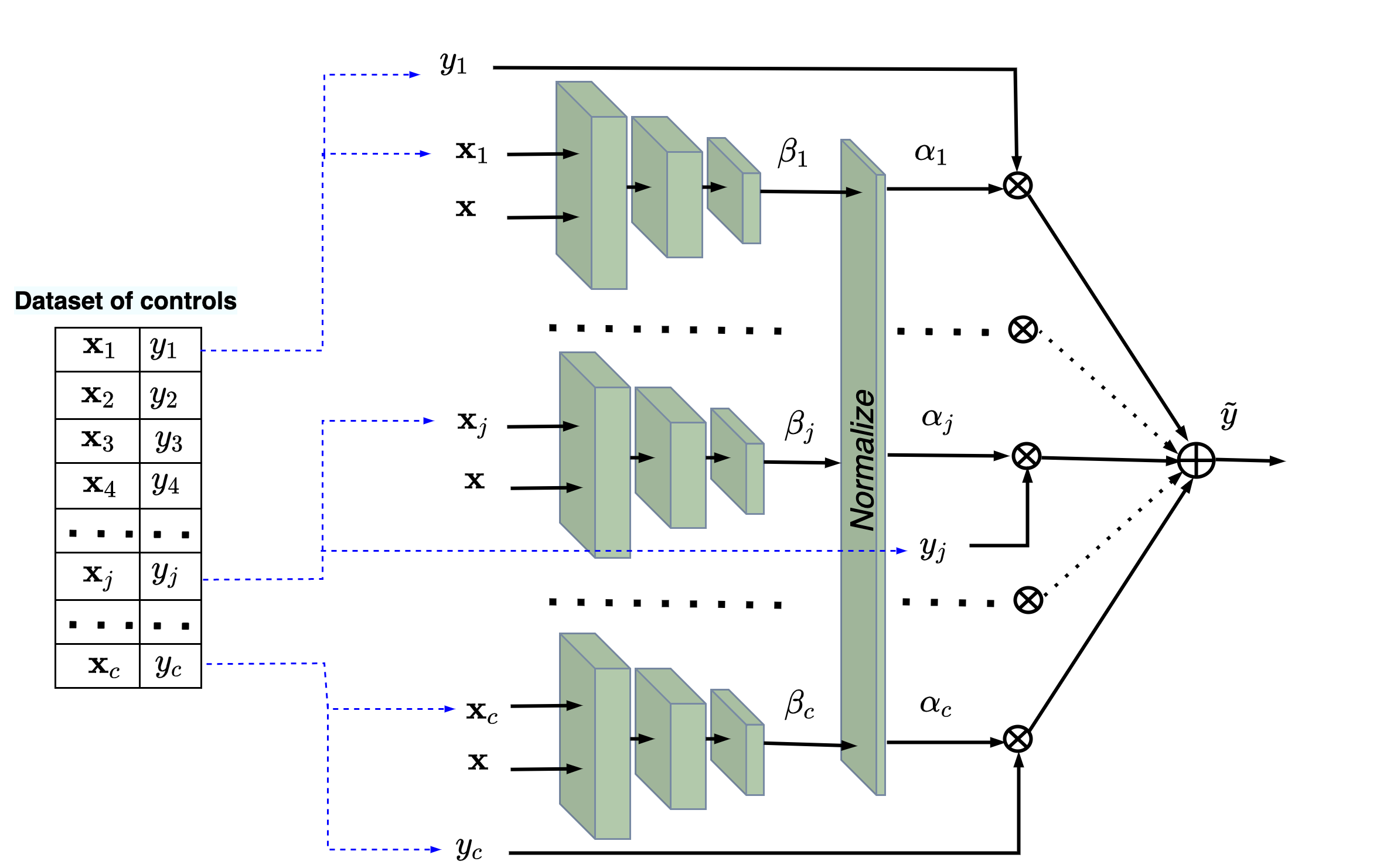
Figure 4: The trained neural network for computing $\tilde{y}$ in accordance with the Nadaraya-Watson regression

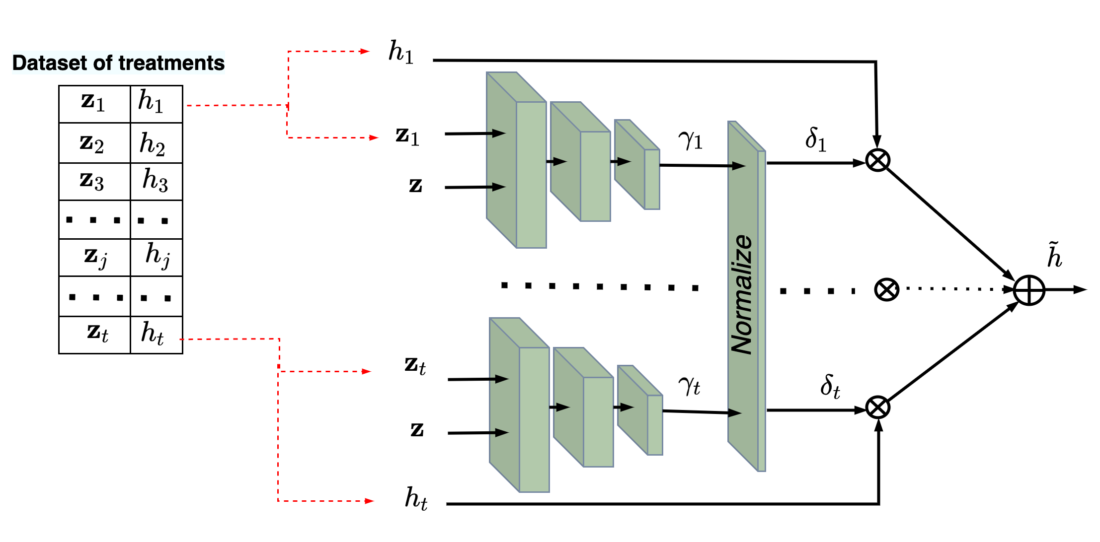
Figure 5: The trained neural network for computing $\tilde{h}$ in accordance with the Nadaraya-Watson regression

The phases of the neural network training and testing are schematically shown as Algorithms 1 and 2, respectively.

Algorithm 1 The algorithm implementing TNW-CATE in the training phase

0:  Datasets $\mathcal{C}$ of $c$ controls and $\mathcal{T}$ of $t$ treatments, numbers $N$ and $M$ of generated subsets of $\mathcal{C}$ and $\mathcal{T}$, numbers of examples in generated subsets $n$ and $m$

0:  The trained weight sharing neural network implementing the Nadaraya-Watson regressions for control and treatment data

1:  for $i=1$, $i\leq c$  do

2:     for $r=1$, $r\leq N$  do

3:        Generate subset $\mathcal{C}_{i,r}\subset\mathcal{C}\backslash(\mathbf{x}_{i},y_{i})$ (see (9))

4:        Form example $\mathbf{a}_{i}^{(r)}$ (see (10))

5:     end for

6:  end for

7:  for $j=1$, $j\leq t$  do

8:     for $s=1$, $s\leq M$  do

9:        Generate subset $\mathcal{T}_{j,s}\subset\mathcal{T}\backslash(\mathbf{z}_{j},h_{j})$ (see (11))

10:        Form example $\mathbf{b}_{j}^{(s)}$ (see (12))

11:     end for

12:  end for

13:  Train the weight sharing neural network with the loss function given in (17) on the set of pairs $(\mathbf{a}_{i}^{(r)},\mathbf{b}_{j}^{(s)})$

Algorithm 2 The algorithm implementing TNW-CATE in the testing phase

0:  Trained neural control and treatment networks implementing the Nadaraya-Watson regressions; datasets $\mathcal{C}$ and $\mathcal{T}$; testing example $\mathbf{x}=\mathbf{z}$

0:  CATE $\tau(\mathbf{x})$

1:  Form the testing example $\mathbf{a}(\mathbf{x})$ in accordance with (18)

2:  Form the testing example $\mathbf{b}(\mathbf{z})$ in accordance with (19)

3:  Feed $\mathbf{a}(\mathbf{x})$ to the control network and $\mathbf{b}(\mathbf{z})$ to the treatment network and get the corresponding predictions $\tilde{y}$ and $\tilde{h}$

4:  $\tau(\mathbf{x})=\tilde{h}-\tilde{y}$

It is important to point out that the neural networks shown in Figs. 4 and 5 are not trained on datasets $\mathcal{C}$ and $\mathcal{T}$. These datasets are used as testing examples. This is an important difference of the proposed approach from other classification or regression models.

Let us return to the case $\alpha=0$ when only the control network is trained on controls without treatments. This case is interesting because it clearly demonstrates the transfer learning model when domains of source and target data are the same, but tasks are different. Indeed, we train kernels of the Nadaraya-Watson regression on controls under assumption that domains of controls and treatments are the same. Kernels learn the feature vector location. Actually, kernels are trained on controls by using outcomes $y_{i}$. However, nothing prevents us from using the same kernels with different outcomes $h_{i}$ if structures of feature vectors in the control and treatment groups are similar. We often use the same standard kernels with the same parameters, for example, Gaussian ones with the temperature parameter, in machine learning tasks. The proposed method does the same, but with a more complex kernel.

5 Numerical experiments

In this section, we provide simulation experiments evaluating the performance of meta-models for CATE estimation. In particular, we compare the T-learner, the S-learner, the X-learner and the proposed method in several simulation studies. Numerical experiments are based on random generation of control and treatment data in accordance with different predefined control and treatment outcome functions because the true CATEs are unknown due to the fundamental problem of the causal inference for real data [8].

5.1 General parameters of experiments

5.1.1 CATE estimators for comparison

The following models are used for their comparison with TNW-CATE.

1. The T-learner [19] is a simple procedure based on estimating the control $g_{0}(\mathbf{x})$ and treatment $g_{1}(\mathbf{z})$ outcome functions by applying a regression algorithm, for example, the random forest [94]. The CATE in this case is defined as the difference $g_{1}(\mathbf{z})-g_{0}(\mathbf{x})$.

2. The S-learner was proposed in [19] to overcome difficulties and disadvantages of the T-learner. The treatment assignment indicator $T_{i}$ in the S-learner is included as an additional feature to the feature vector $\mathbf{x}$. The corresponding training set in this case is modified as $\mathcal{D}^{\ast}=\{(\mathbf{x}_{1}^{\ast},y_{1}),...,(\mathbf{x}_{c+t}^{\ast},y_{c+t})\}$, where $\mathbf{x}_{i}^{\ast}=(\mathbf{x}_{i},T_{i})\in\mathbb{R}^{d+1}$ if $T_{i}=0$, $i=1,...,c$, and $\mathbf{x}_{c+i}^{\ast}=(\mathbf{z}_{i},T_{i})\in\mathbb{R}^{d+1}$ if $T_{i}=1$, $i=1,...,t$. Then the outcome function $g(\mathbf{x},T)$ is estimated by using the training set $\mathcal{D}^{\ast}$. The CATE is determined in this case as $\tau(\mathbf{x})=g(\mathbf{x},1)-g(\mathbf{x},0).$

3. The X-learner [19] is based on computing the so-called imputed treatment effects and is represented in the following three steps. First, the outcome functions $g_{0}(\mathbf{x})$ and $g_{1}(\mathbf{z})$ are estimated using a regression algorithm, for example, the random forest. Second, the imputed treatment effects are computed as follows:

   $$D_{1}(\mathbf{z}_{i})=h_{i}-g_{0}(\mathbf{z}_{i}),\ \ D_{0}(\mathbf{x}_{i})=g_{1}(\mathbf{x}_{i})-y_{i}.$$ (21)

   Third, two regression functions $\tau_{1}(\mathbf{z})$ and $\tau_{0}(\mathbf{x})$ are estimated for imputed treatment effects $D_{1}(\mathbf{z}_{i})$ and $D_{0}(\mathbf{x}_{i})$, respectively. CATE for a point $\mathbf{x}=\mathbf{z}$ is defined as a weighted linear combination of the functions $\tau_{1}(\mathbf{z})$ and $\tau_{0}(\mathbf{x})$ as $\tau(\mathbf{x})=\alpha\tau_{0}(\mathbf{x})+(1-\alpha)\tau_{1}(\mathbf{x})$, where $\alpha\in[0,1]$ is a weight which is equal to the ratio of treated patients [8].

5.1.2 Base models for implementing estimators

Two models are used as the base regressors $g_{0}(\mathbf{x})$ and $g_{1}(\mathbf{z})$, which realize different CATE estimators for comparison purposes.

1. The first one is the random forest. It is used as the base regressor to implement other models due to two main reasons. First, we consider the case of the small number of treatments, and usage of neural networks does not allow us to obtain the desirable accuracy of the corresponding regressors. Second, we deal with tabular data for which it is difficult to train a neural network and the random forest is preferable. Parameters of random forests used in experiments are the following:

   • numbers of trees are 10, 50, 100, 300;

   • depths are 2, 3, 4, 5, 6, 7;

   • the smallest values of examples which fall in a leaf are 1 example, 5%, 10%, 20% of the training set.

   The above values for the hyperparameters are tested, choosing those leading to the best results.

2. The second base model used for realization different CATE estimators is the Nadaraya-Watson regression with the standard Gaussian kernel. This model is used because it is interesting to compare it with the proposed model which is also based on the Nadaraya-Watson regression but with the trainable kernel in the form of the neural network of the special form. Values $10^{i}$, $i=-8,...,10$, and also values $0.5$, $5$, $50$, $100$, $200$, $500$, $700$ of the bandwidth parameter $\gamma$ are tested, choosing those leading to the best results.

We use the following notation for different models depending on the base models and learners:

• T-RF, S-RF, X-RF are the T-learner, the S-learner, the X-learner with random forests as the base regression models;

• T-NW, S-NW, X-NW are the T-learner, the S-learner, the X-learner with the Nadaraya-Watson regression using the standard Gaussian kernel as the base regression models.

5.1.3 Other parameters of numerical experiments

The mean squared error (MSE) as a measure of the regression model accuracy is used. For estimating MSE, we perform several iterations of experiments such that each iteration is defined by the randomly selected parameters of experiments. MSE is computed by using 1000 points. In all experiments, the number of treatments is $10\%$ of the number of controls. For example, if $100$ controls are generated for an experiment, then $10$ treatments are generated in addition to controls such that the total number of examples is $110$. After generating training examples, their responses $y$ are normalized, but the corresponding initial mean and the standard deviation of responses are used to normalize responses of the test examples. This procedure allows us to reduce the variance among results at different iterations. The generated feature vectors in all experiments consist of $10$ features. To select optimal hyperparameters of all regressors, additional validation examples are generated such that the number of controls is $20\%$ of the training examples from the control group. The validation examples are not used for training.

5.1.4 Functions for generating datasets

The following functions are used to generate synthetic datasets:

1. Spiral functions: The functions are named spiral because for the case of two features vectors are located on the Archimedean spiral. For even $d$, we write the vector of features as

   $$\mathbf{x}=(t\sin(t),t\cos(t),...,t\sin(t\cdot d/2),t\cos(t\cdot d/2)).$$ (22)

   For odd $d$, there holds

   $$\mathbf{x}=(t\sin(t),t\cos(t),...,t\sin(t\cdot\left\lceil d/2\right\rceil)).$$ (23)

   The responses are generated as a linear function of $t$, i.e., they are computed as $y=at+b$.

   Values of parameters $a$, $b$ and $t$ for performing numerical experiments with spiral functions are the following:

   • The control group: parameters $a$, $b$, $t$ are uniformly generated from intervals $[1,4]$, $[1,4]$, $[0,10]$, respectively.

   • The treatment group: parameters $a$, $b$, $t$ are uniformly generated from intervals $[8,10]$, $[8,10]$, $[0,10]$, respectively.

2. Logarithmic functions: Features are logarithms of the parameter $t$, i.e., there holds

   $$\mathbf{x}=(a_{1}\ln(t),a_{2}\ln(t),...,a_{d}\ln(t)).$$ (24)

   The responses are generated as a logarithmic function with adding an oscillating term $b\sin(t)$ to $y$, i.e., there holds $y=b(\ln(t)+\sin(t))$.

   Values of parameters $a_{1},...,a_{d}$, $b$ for performing numerical experiments with logarithmic functions are the following:

   • Each parameter from the set $\{a_{1},...,a_{d}\}$ is uniformly generated from intervals $[-4,-1]\cup[1,4]$ for controls as well as for treatments.

   • Parameter $b$ is uniformly generated from interval $[1,4]$ for controls and from interval $[-4,-1]$ for treatments.

   • Values of $t$ are uniformly generated in interval $[0.5,5]$.

3. Power functions: Features are represented as powers of $t$. For arbitrary $d$, the vector of features is represented as

   $$\mathbf{x}=(t^{1/\sqrt{d}},t^{2/\sqrt{d}},...,t^{d/\sqrt{d}}).$$ (25)

   However, features which are close to linear ones, i.e., $x_{i}=t^{i/\sqrt{d}}$ for $0.8<i/\sqrt{d}<1.6$, are replaced with the Gaussian noise having the unit standard deviation and the zero expectation, i.e., $x_{i}\sim\mathcal{N}(0,1)$. The responses are generated as follows:

   $$y=a\cdot\exp\left(-\frac{(t-s)^{2}}{b}\right).$$ (26)

   Values of parameters $a$, $b$, $s$, $t$ for performing numerical experiments with power functions are the following:

   • The control group: parameters $a$ and $b$ are uniformly generated from intervals $[1,2]$ and $[0.25,1]$, respectively; parameter $s$ is $2.5$.

   • The treatment group: parameters $a$ and $b$ are uniformly generated from intervals $[2,4]$ and $[1,2]$, respectively; parameter $s$ is $2.5$.

   • Values of $t$ are uniformly generated in interval $[0,5]$.

4. Indicator functions [19]: The functions are expressed through the indicator function $I$ taking value $1$ if its argument is true.

   • The function for controls is represented as

     $$g_{0}(\mathbf{x})=\mathbf{x}^{\mathrm{T}}\beta+5I(x_{1}>0.5).$$ (27)

   • The function for treatments is represented as

     $$g_{1}(\mathbf{x})=\mathbf{x}^{\mathrm{T}}\beta+5I(x_{1}>0.5)+8I(x_{2}>0.1).$$ (28)

   • Vector $\beta$ is uniformly distributed in interval $[-5;5]^{d}$; values of features $x_{i}=1,...,d$, are uniformly generated from interval $[-1,1]$.

The indicator function differs from other functions considered in numerical examples. It is taken from [19] to study TNW-CATE when the assumption of specific and similar domains for the control and treatment feature vectors can be violated.

In numerical experiments with the above functions, we take parameter $\alpha$ equal to $0.1$, $0.5$, $0.5$ and $0.5$ for the spiral, logarithmic, power and indicator functions, respectively, except for experiments which study how parameter $\alpha$ impacts on the MSE.

5.2 Study of the TNW-CATE properties

In all pictures illustrating dependencies of CATE estimators on parameters of models, dotted curves correspond to the T-learner, the S-learner, the X-learner implemented by using the Nadaraya-Watson regression (triangle markers correspond to T-NW and S-NW, the circle marker corresponds to X-NW). Dashed curves with the same markers correspond to the same models implemented by using RFs. The solid curve with cross markers corresponds to TNW-CATE.

5.2.1 Experiments with numbers of training data

Let us compare different CATE estimators by different numbers of control and treatment examples. We study the estimators by numbers $c$ of controls: $100$, $250$, $500$, $750$, $1000$. Each number of treatments is determined as $10\%$ of each number of controls. Value $n$ is $80$ and $100$, value $m$ is $50\%$ of $t$. Fig. 6 illustrates how MSE of the CATE values depends on the number $c$ of controls for different estimators when different functions are used for generating examples. In fact, these experiments study how MSE depends on the whole number of controls and treatments because the number of treatments increases with the number of controls. For all functions, the increase of the amount of training examples improves most estimators including TNW-CATE. These results are expectable because the larger size of training data mainly leads to the better accuracy of models. It can be seen from Fig. 6 that the proposed model provides better results in comparison with other models. The best results are achieved when the spiral generating function is used. The models different from TNW-CATE cannot cope with the complex structure of data in this case. However, TNW-CATE shows comparative results with the T-learner, the S-learner, the X-learner when the indicator function is used for generating examples. The X-learner outperforms TNW-CATE in this case. The indicator function does not have a complex structure. Moreover, the corresponding outcomes linearly depend on most features (see (27)-(28)) and random forests implementing X-RF are trained better than the neural network implementing TNW-CATE. One can also see from Fig. 6 that models T-NW, S-NW, X-NW based on the Nadaraya-Watson regression with the Gaussian kernel provide close results when the logarithmic generating function is used by larger numbers of training data. This is caused by the fact that the Gaussian kernel is close to the neural network kernel implemented in TNW-CATE.

Fig. 7 illustrates how the number of controls impacts separately on the control (the left plot) and treatment (the right plot) regressions when the power function is used for generating data. It can be also seen from Fig. 7 that MSE provided by the control network is much smaller than MSE of the treatment neural network.

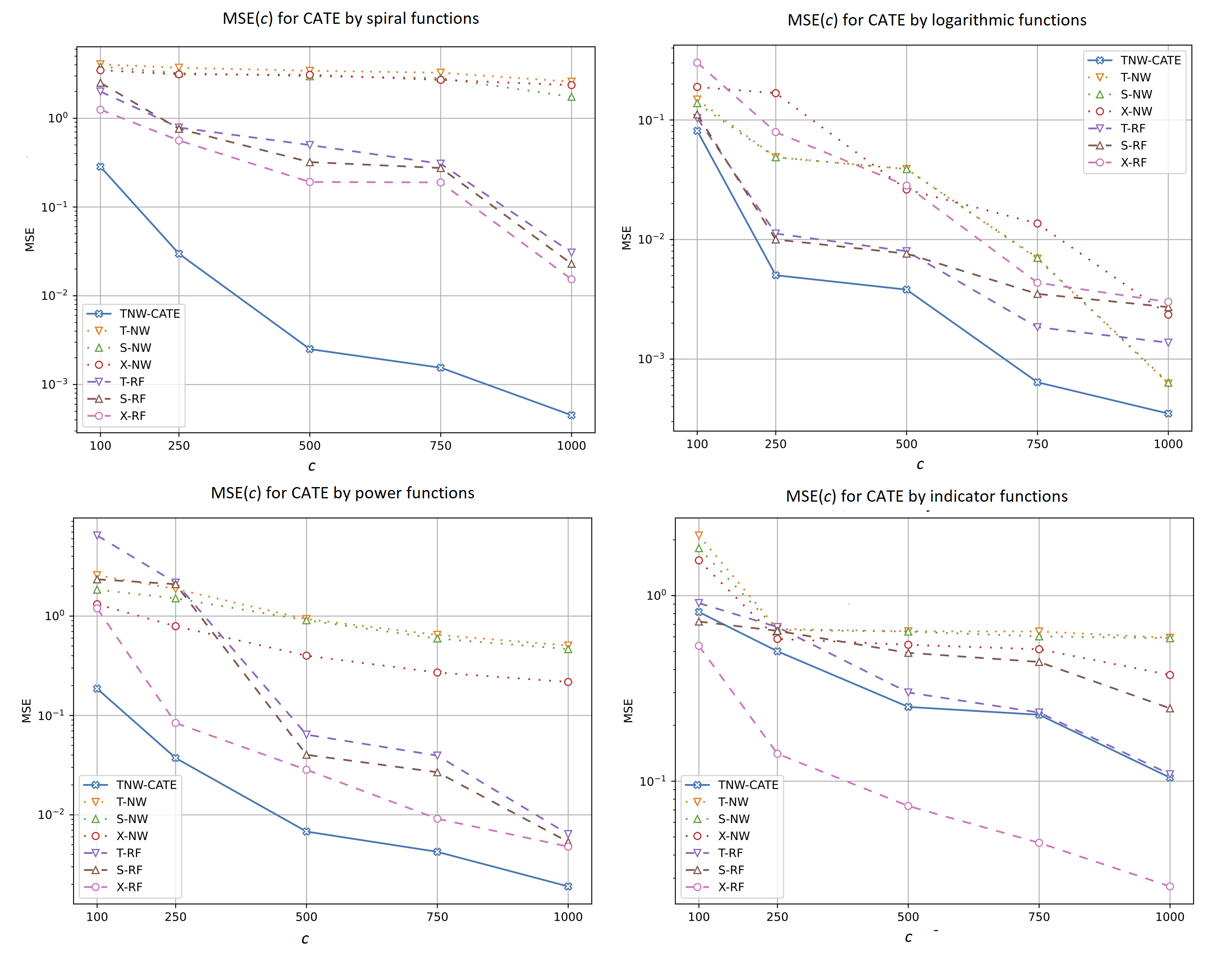
Figure 6: MSE of the CATE values as a function of the number of controls when spiral, logarithmic, power and indicator functions are used for generating examples

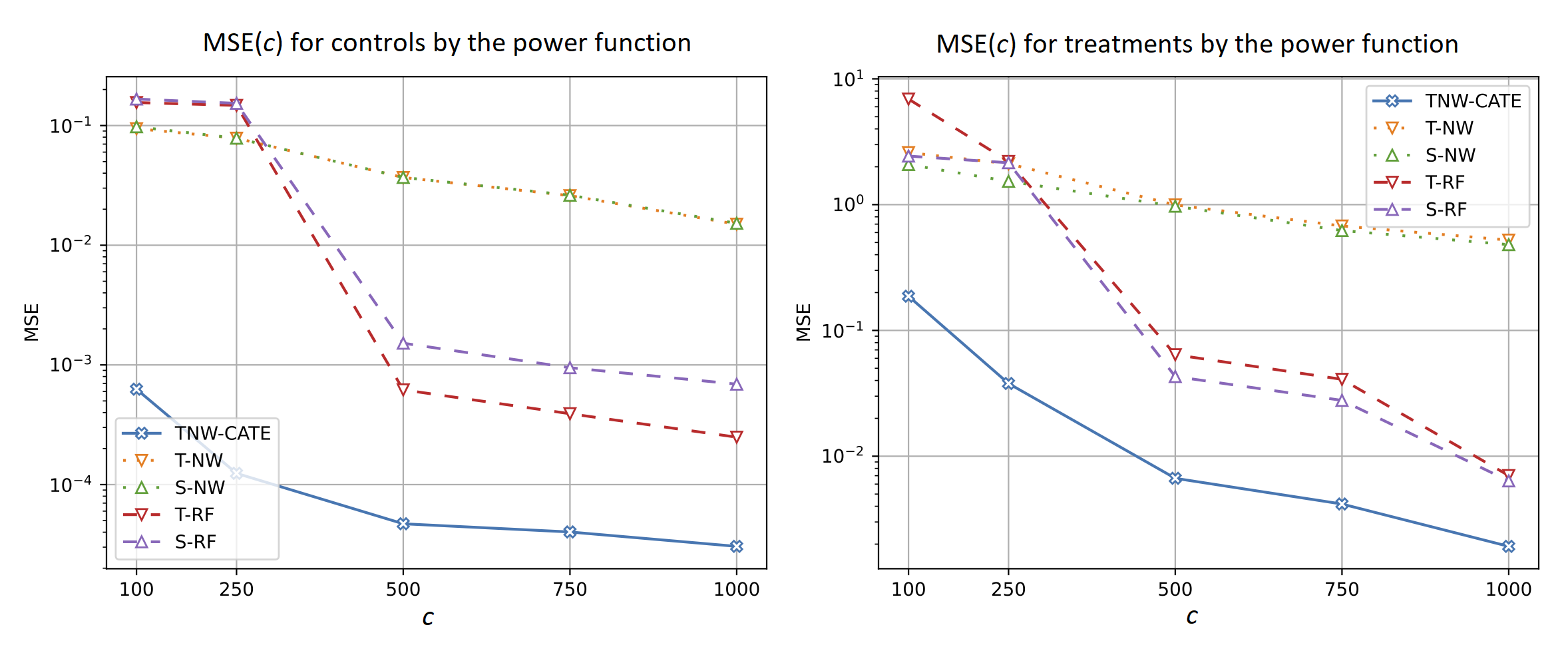
Figure 7: MSE of the control (the left plot) and treatment (the right plot) responses as functions of the number of controls when the power function is used for generating examples

5.2.2 Experiments with different values of the treatment ratio

Another question is how the CATE estimators depend on the ratio of numbers of treatments and controls in the training set. We study the case when the number of controls $c$ is $200$ and the ratio takes values from the set $\{0.1,0.2,0.3,0.4,0.5\}$. The coefficient $\alpha$ is taken in accordance with the certain function as described above.

Similar results are shown in Fig. 8 where plots of MSE of the CATE values as a function of the ratio of numbers of treatments in the training set by different generating functions are depicted. We again see from Fig. 8 that the difference between MSE of TNW-CATE and other models is largest when the spiral function is used. TNW-CATE also provides better results in comparison with other models, except for the case of the indicator function when is TNW-CATE inferior to the X-RF.

Fig. 9 illustrates how the ratio of numbers of treatments impacts separately on the control (the left plot) and treatment (the right plot) regressions when the logarithmic function is used for generating data. It can be seen from Fig. 9 that MSE of the treatment network is very close to MSE of other models almost for all values of the ratio, but the accuracy of the control network significantly differs from other model.

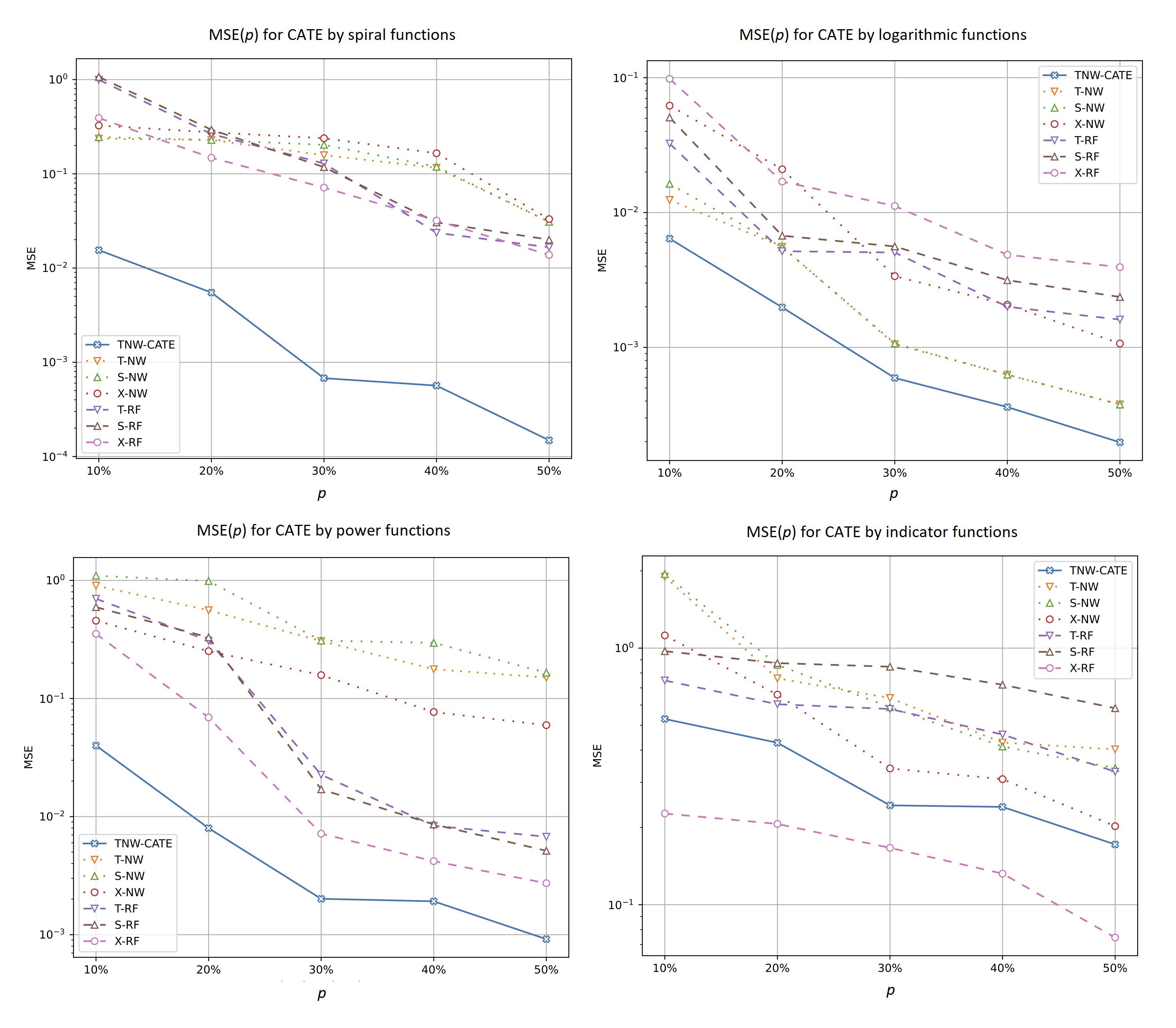
Figure 8: MSE of the CATE values as a function of the ratio of numbers of treatments in the training set when spiral, logarithmic, power and indicator functions are used for generating examples

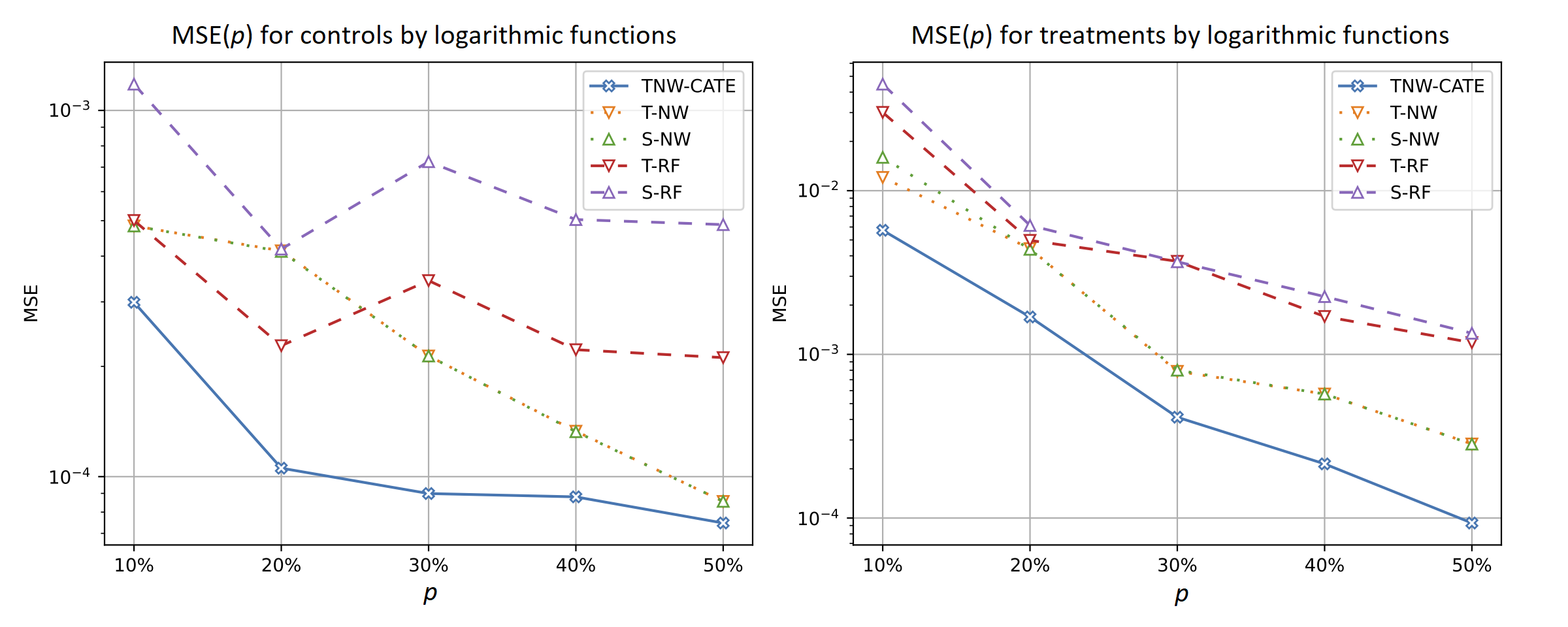
Figure 9: MSE of the control (the left plot) and treatment (the right plot) responses as functions of the ratio of numbers of treatments in the training set when the logarithmic function is used for generating examples

5.2.3 Experiments with different values of $\alpha$

The next experiments allow us to investigate how the CATE estimators depend on the value of hyperparameter $\alpha$ which controls the impact of the control and treatment networks in the loss function (17). The corresponding numerical results are shown in Figs. 10-11. It should be noted that other models do not depend on $\alpha$. One can see from Figs. 10-11 that there is an optimal value of $\alpha$ minimizing MSE of TNW-CATE for every generating function. For example, the optimal $\alpha$ for the spiral function is $0.1$. It can be seen from Fig. 10 that TNW-CATE can be inferior to other models when $\alpha$ is not optimal. For example, the case $\alpha=0$ for the logarithmic function leads to worse results of TNW-CATE in comparison with T-RF and S-RF.

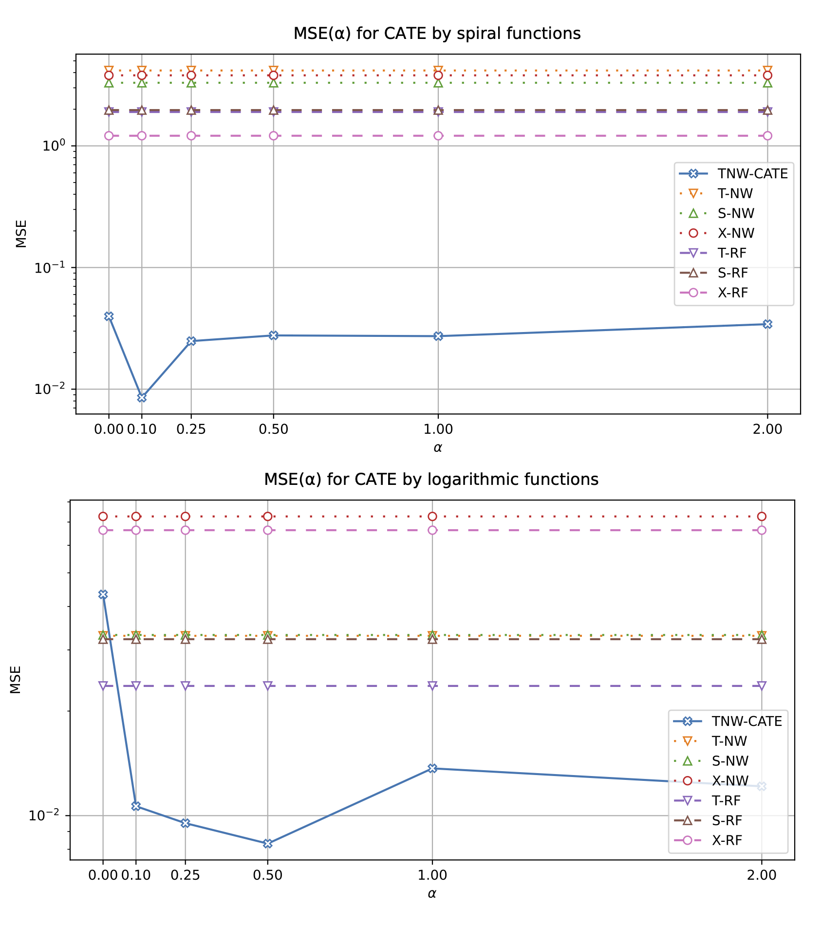
Figure 10: MSE of the CATE values as a function of the coefficient $\alpha$ when spiral (the first plot) and logarithmic (the second plot) functions are used for generating examples

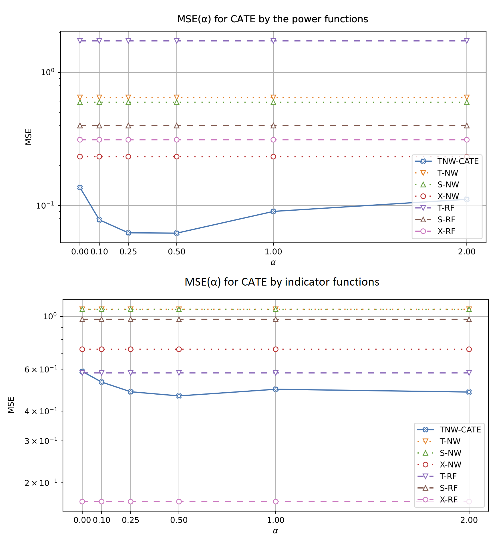
Figure 11: MSE of the CATE values as a function of the coefficient $\alpha$ when power (the first plot) and indicator (the second plot) functions are used for generating examples

Numerical results are also presented in Table 1 where the MSE values corresponding to different models by different generating functions are given. The best results for every function are shown in bold. It can be seen from Table 1 that TNW-CATE provides the best results for the spiral, logarithmic and power functions. Moreover, the improvement is sufficient. TNW-CATE is comparable with the X-NW and X-RF by the logarithmic and power generating functions. At the same time, the proposed model is inferior to X-RF for the indicator function.

Table 1: The best MSE values of CATE for different models and by different generating functions

	Functions
Model	Spiral	Logarithmic	Power	Indicator
T-NW	$3.806$	$0.377$	$1.722$	$0.650$
S-NW	$3.629$	$0.341$	$1.719$	$0.549$
X-NW	$3.279$	$0.542$	$0.632$	$0.353$
T-RF	$2.278$	$0.051$	$2.743$	$0.337$
S-RF	$2.575$	$0.060$	$0.839$	$0.434$
X-RF	$1.385$	$0.202$	$0.805$	$\mathbf{0.061}$
TNW-CATE	$\mathbf{0.232}$	$\mathbf{0.026}$	$\mathbf{0.353}$	$0.257$

It is important to point out that application of many methods based on neural networks, for example, DRNet [65], DragonNet [66], FlexTENet [59] and VCNet [62], to comparing them with TNW-CATE have not been successful because the aforementioned neural networks require the large amount of data for training and the considered small datasets have led to the network overfitting. Therefore, we considered models for comparison, which are based on methods dealing with small data.

6 Conclusion

A new method (TNW-CATE) for solving the CATE problem has been studied. The main idea behind TNW-CATE is to use the Nadaraya-Watson regression with kernels which are implemented as neural networks of the considered specific form and are trained on many randomly selected subsets of the treatment and control data. With the proposed method, we aimed to avoid constructing the regression function $g_{1}$ based only on the treatment group because it may be small. Moreover, we aimed to avoid using standard kernels, for example, Gaussian ones, in the Nadaraya-Watson regression. By training kernels on controls (or controls and treatments), we aimed to transfer knowledge of the feature vector structure in the control group to the treatment group.

In spite of the apparent complexity of the whole neural network for training, TNW-CATE is actually simple because it can be realized as a single small subnetwork implementing the kernel.

Numerical simulation experiments have illustrated the outperformance of TNW-CATE for several datasets.

We used neural networks to learn kernels in the Nadaraya-Watson regression. However, different models can be applied to the kernel implementation, for example, the random forest [94] or the gradient boosting machine [95]. The study of different models for estimating CATE is a direction for further research. We also assumed the similarity between structures of control and treatment data. This assumption can be violated in some cases. Therefore, it is interesting to modify TNW-CATE to take into account the violation. This is another direction for further research. Another interesting direction for research is to incorporate robust procedures and imprecise statistical models to deal with small datasets into TNW-CATE. The incorporation of the models can provide estimates of CATE, which are more robust than estimates obtained by means of TNW-CATE.

References

- [1] M. Lu, S. Sadiq, D.J. Feaster, and H. Ishwaran. Estimating individual treatment effect in observational data using random forest methods. arXiv:1701.05306v2, Jan 2017.
- [2] U. Shalit, F.D. Johansson, and D.A. Sontag. Estimating individual treatment effect: generalization bounds and algorithms. In Proceedings of the 34th International Conference on Machine Learning (ICML 2017), volume PMLR 70, pages 3076–3085, Sydney, Australia, 2017.
- [3] Y. Fan, J. Lv, and J. Wang. DNN: A two-scale distributional tale of heterogeneous treatment effect inference. arXiv:1808.08469v1, Aug 2018.
- [4] D.P. Green and H.L Kern. Modeling heterogeneous treatment effects in survey experiments with Bayesian additive regression trees. Public Opinion Quarterly, 76(3):491–511, 2012.
- [5] J.L. Hill. Bayesian nonparametric modeling for causal inference. Journal of Computational and Graphical Statistics, 20(1), 2011.
- [6] N. Kallus. Learning to personalize from observational data. arXiv:1608.08925, 2016.
- [7] S. Wager and S. Athey. Estimation and inference of heterogeneous treatment effects using random forests. arXiv:1510.0434, 2015.
- [8] S.R. Kunzel, B.C. Stadie, N. Vemuri, V. Ramakrishnan, J.S. Sekhon, and P. Abbeel. Transfer learning for estimating causal effects using neural networks. arXiv:1808.07804v1, Aug 2018.
- [9] T. Wendling, K. Jung, A. Callahan, A. Schuler, N.H. Shah, and B. Gallego. Comparing methods for estimation of heterogeneous treatment effects using observational data from health care databases. Statistics in Medicine, pages 1–16, 2018.
- [10] arXiv:2205.14714. Heterogeneous treatment effects estimation: When machine learning meets multiple treatment regime. N. Acharki and J. Garnier and A. Bertoncello and R. Lugo, May 2022.
- [11] Ahmed Alaa and Mihaela van der Schaar. Limits of estimating heterogeneous treatment effects: Guidelines for practical algorithm design. In Proceedings of the 35th International Conference on Machine Learning, volume 80 of Proceedings of Machine Learning Research, pages 129–138, Stockholmsmässan, Stockholm Sweden, 2018. PMLR.
- [12] S. Athey and G. Imbens. Recursive partitioning for heterogeneous causal effects. Proceedings of the National Academy of Sciences, pages 1–8, 6 2016.
- [13] A. Deng, P. Zhang, S. Chen, D.W. Kim, and J. Lu. Concise summarization of heterogeneous treatment effect using total variation regularized regression. arXiv:1610.03917, Oct 2016.
- [14] C. Fernandez-Loria and F. Provost. Causal classification: Treatment effect estimation vs. outcome prediction. Journal of Machine Learning Research, 23:1–35, 2022.
- [15] C. Fernandez-Loria and F. Provost. Causal decision making and causal effect estimation are not the same…and why it matters. INFORMS Journal on Data Science, pages 1–14, 2022.
- [16] Xiajing Gong, Meng Hu, M. Basu, and Liang Zhao. Heterogeneous treatment effect analysis based on machine-learning methodology. CPT: Pharmacometrics & Systems Pharmacology, 10:1433–1443, 2021.
- [17] T. Hatt, J. Berrevoets, A. Curth, S. Feuerriegel, and M. van der Schaar. Combining observational and randomized data for estimating heterogeneous treatment effects. arXiv:2202.12891, Feb 2022.
- [18] Hao Jiang, Peng Qi, Jingying Zhou, Jack Zhou, and Sharath Rao. A short survey on forest based heterogeneous treatment effect estimation methods: Meta-learners and specific models. In 2021 IEEE International Conference on Big Data (Big Data), pages 3006–3012. IEEE, 2021.
- [19] S.R. Kunzel, J.S. Sekhona, P.J. Bickel, and B. Yu. Meta-learners for estimating heterogeneous treatment effects using machine learning. Proceedings of the National Academy of Sciences, 116(10):4156–4165, 2019.
- [20] S.R. Kunzel, J.S. Sekhon, P.J. Bickel, and Bin Yu. Metalearners for estimating heterogeneous treatment effects using machine learning. PNAS, 116(10):4156–4165, 2019.
- [21] L.V. Utkin, M.V. Kots, V.S. Chukanov, A.V. Konstantinov, and A.A. Meldo. Estimation of personalized heterogeneous treatment effects using concatenation and augmentation of feature vectors. International Journal on Artificial Intelligence Tools, 29(5):1–23, 2020. Article 2050005.
- [22] Lili Wu and Shu Yang. Integrative learner of heterogeneous treatment effects combining experimental and observational studies. In Proceedings of the First Conference on Causal Learning and Reasoning (CLeaR 2022), pages 1–23, https://openreview.net/pdf?id=Q102xPpYV-B, 2022.
- [23] S. Yadlowsky, S. Fleming, N. Shah, E. Brunskill, and S. Wager. Evaluating treatment prioritization rules via rank-weighted average treatment effects. arXiv:2111.07966, Nov 2021.
- [24] Weijia Zhang, Jiuyong Li, and Lin Liu. A unified survey of treatment effect heterogeneity modelling and uplift modelling. ACM Computing Surveys, 54(8):1–36, 2022.
- [25] Y. Zhao, D. Zeng, A.J. Rush, and M.R. Kosorok. Estimating individualized treatment rules using outcome weighted learning. Journal of the American Statistical Association, 107(449):1106–1118, 2012.
- [26] I. Bica, J. Jordon, and M. van der Schaar. Estimating the effects of continuous-valued interventions using generative adversarial networks. In Advances in neural information processing systems (NeurIPS), volume 33, pages 16434–16445, 2020.
- [27] A. Curth and M. van der Schaar. Nonparametric estimation of heterogeneous treatment effects: From theory to learning algorithms. In International Conference on Artificial Intelligence and Statistics, pages 1810–1818. PMLR, 2021.
- [28] U. Shalit, F.D. Johansson, and D. Sontag. Estimating individual treatment effect: generalization bounds and algorithms. In International Conference on Machine Learning, pages 3076–3085, 2017.
- [29] Zhenyu Guo, Shuai Zheng, Zhizhe Liu, Kun Yan, and Zhenfeng Zhu. Cetransformer: Casual effect estimation via transformer based representation learning. In Pattern Recognition and Computer Vision. PRCV 2021, volume 13022 of Lecture Notes in Computer Science, pages 524–535. Springer, Cham, 2021.
- [30] V. Melnychuk, D. Frauen, and S. Feuerriegel. Causal transformer for estimating counterfactual outcomes. arXiv:2204.07258, Apr 2022.
- [31] Yi-Fan Zhang, Hanlin Zhang, Z.C. Lipton, Li Erran Li, and Eric P. Xing. Can transformers be strong treatment effect estimators? arXiv:2202.01336, Feb 2022.
- [32] Yi-Fan Zhang, Hanlin Zhang, Z.C. Lipton, Li Erran Li, and Eric P. Xing. Exploring transformer backbones for heterogeneous treatment effect estimation. arXiv:2202.01336, May 2022.
- [33] E.A. Nadaraya. On estimating regression. Theory of Probability & Its Applications, 9(1):141–142, 1964.
- [34] G.S. Watson. Smooth regression analysis. Sankhya: The Indian Journal of Statistics, Series A, pages 359–372, 1964.
- [35] P.L. Bartlett, A. Montanari, and A. Rakhlin. Deep learning: a statistical viewpoint. Acta Numerica, 30:87–201, 2021.
- [36] J. Lu, V. Behbood, P. Hao, H. Zuo, S. Xue, and G. Zhang. Transfer learning using computational intelligence: A survey. Knowledge-Based Systems, 80:14–23, 2015.
- [37] S. Pan and Q. Yang. A survey on transfer learning. IEEE Trans. on Knowledge and Data Engineering, 22(10):1345–1359, 2010.
- [38] K. Weiss, T.M. Khoshgoftaar, and D. Wang. A survey of transfer learning. Journal of Big Data, 3(1):1–40, 2016.
- [39] S. Powers, J. Qian, K. Jung, A. Schuler, N.H. Shah, T. Hastie, and R. Tibshirani. Some methods for heterogeneous treatment effect estimation in high-dimensions some methods for heterogeneous treatment effect estimation in high-dimensions. arXiv:1707.00102v1, Jul 2017.
- [40] X.J. Jeng, W. Lu, and H. Peng. High-dimensional inference for personalized treatment decision. Electronic Journal of Statistics, 12:12 2074–2089, 2018.
- [41] X. Zhou, N. Mayer-Hamblett, U. Khan, and M.R. Kosorok. Residual weighted learning for estimating individualized treatment rules. Journal of the American Statistical Association, 112(517):169–187, 2017.
- [42] S. Athey, J. Tibshirani, and S. Wager. Solving heterogeneous estimating equations with gradient forests. arXiv:1610.01271, Oct 2016.
- [43] S. Athey, J. Tibshirani, and S. Wager. Generalized random forests. arXiv:1610.0171v4, Apr 2018.
- [44] W. Zhang, T.D. Le, L. Liu, Z.-H. Zhou, and J. Li. Mining heterogeneous causal effects for personalized cancer treatment. Bioinformatics, 33(15):2372–2378, 2017.
- [45] Y. Xie, N. Chen, and X. Shi. False discovery rate controlled heterogeneous treatment effect detection for online controlled experiments. arXiv:1808.04904v1, Aug 2018.
- [46] M. Oprescu, V. Syrgkanis, and Z.S. Wu. Orthogonal random forest for heterogeneous treatment effect estimation. arXiv:1806.03467v2, Jul 2018.
- [47] E. McFowland III, S. Somanchi, and D.B. Neill. Efficient discovery of heterogeneous treatment effects in randomized experiments via anomalous pattern detection. arXiv:1803.09159v2, Jun 2018.
- [48] R. Chen and H. Liu. Heterogeneous treatment effect estimation through deep learning. arXiv:1810.11010v1, Oct 2018.
- [49] J. Grimmer, S. Messing, and S.J. Westwood. Estimating heterogeneous treatment effects and the effects of heterogeneous treatments with ensemble methods. Political Analysis, 25(4):413–434, 2017.
- [50] N. Kallus, A.M. Puli, and U. Shalit. Removing hidden confounding by experimental grounding. arXiv:1810.11646v1, Oct 2018.
- [51] N. Kallus and A. Zhou. Confounding-robust policy improvement. arXiv:1805.08593v2, Jun 2018.
- [52] M.C. Knaus, M. Lechner, and A. Strittmatter. Machine learning estimation of heterogeneous causal effects: Empirical monte carlo evidence. arXiv:1810.13237v1, Oct 2018.
- [53] S.R. Kunzel, S.J.S. Walter, and J.S. Sekhon. Causaltoolbox - estimator stability for heterogeneous treatment effects. arXiv:1811.02833v1, Nov 2018.
- [54] J. Levy, M. van der Laan, A. Hubbard, and R. Pirracchio. A fundamental measure of treatment effect heterogeneity. arXiv:1811.03745v1, Nov 2018.
- [55] W. Rhodes. Heterogeneous treatment effects: What does a regression estimate? Evaluation Review, 34(4):334–361, 2010.
- [56] Y. Xie, J.E. Brand, and B. Jann. Estimating heterogeneous treatment effects with observational data. Sociological methodology, 42(1):314–347, 2012.
- [57] L. Yao, C. Lo, I. Nir, S. Tan, A. Evnine, A. Lerer, and A. Peysakhovich. Efficient heterogeneous treatment effect estimation with multiple experiments and multiple outcomes. arXiv:2206.04907, Jun 2022.
- [58] Y. Wang, P. Wu, Y. Liu, C. Weng, and D. Zeng. Learning optimal individualized treatment rules from electronic health record data. In IEEE International Conference on Healthcare Informatics (ICHI), pages 65–71. IEEE, 2016.
- [59] A. Curth and M. van der Schaar. On inductive biases for heterogeneous treatment effect estimation. In 35th Conference on Neural Information Processing Systems (NeurIPS 2021), pages 1–12, 2021.
- [60] Xinze Du, Yingying Fan, Jinchi Lv, Tianshu Sun, and P. Vossler. Dimension-free average treatment effect inference with deep neural networks. arXiv:2112.01574, Dec 2021.
- [61] N. Nair, K.S. Gurumoorthy, and D. Mandalapu. Individual treatment effect estimation through controlled neural network training in two stages. arXiv:2201.08559, Jan 2022.
- [62] Lizhen Nie, Mao Ye, Qiang Liu, and D. Nicolae. Vcnet and functional targeted regularization for learning causal effects of continuous treatments. In International Conference on Learning Representations (ICLR 2021), pages 1–24, 2021.
- [63] S. Parbhoo, S. Bauer, and P. Schwab. Ncore: Neural counterfactual representation learning for combinations of treatments. arXiv:2103.11175, Mar 2021.
- [64] Tian Qin, Tian-Zuo Wang, and Zhi-Hua Zhou. Budgeted heterogeneous treatment effect estimation. In Proceedings of the 38th International Conference on Machine Learning, PMLR, volume 139, pages 8693–8702, 2021.
- [65] P. Schwab, L. Linhardt, S. Bauer, J.M. Buhmann, and W. Karlen. Learning counterfactual representations for estimating individual dose-response curves. In Proceedings of the AAAI Conference on Artificial Intelligence, volume 34, pages 5612–5619, 2020.
- [66] Claudia Shi, D. Blei, and V. Veitch. Adapting neural networks for the estimation of treatment effects. In Advances in Neural Information Processing Systems, volume 32, pages 1–11. Curran Associates, Inc., 2019.
- [67] V. Veitch, Yixin Wang, and D.M. Blei. Using embeddings to correct for unobserved confounding in networks. In 33rd Conference on Neural Information Processing Systems (NeurIPS 2019), pages 1–11, 2019.
- [68] S. Chaudhari, V. Mithal, G. Polatkan, and R. Ramanath. An attentive survey of attention models. arXiv:1904.02874, Apr 2019.
- [69] R. Aoki and M. Ester. Causal inference from small high-dimensional datasets. arXiv:2205.09281, May 2022.
- [70] Wenshuo Guo, Serena Wang, Peng Ding, Yixin Wang, and M.I. Jordan. Multi-source causal inference using control variates. arXiv:2103.16689, Mar 2021.
- [71] S.R. Kunzel, B.C. Stadie, N. Vemuri, V. Ramakrishnan, J.S. Sekhon, and P. Abbeel. Transfer learning for estimating causal effects using neural networks. arXiv:1808.07804, Aug 2018.
- [72] G.W. Imbens. Nonparametric estimation of average treatment effects under exogeneity: A review. Review of Economics and Statistics, 86(1):4–29, 2004.
- [73] J. Park, U. Shalit, B. Scholkopf, and K. Muandet. Conditional distributional treatment effect with kernel conditional mean embeddings and u-statistic regression. In Proceedings of the 38 th International Conference on Machine Learning, PMLR, volume 139, pages 8401–8412, 2021.
- [74] Y.A. Ghassabeh and F. Rudzicz. The mean shift algorithm and its relation to kernel regression. Information Sciences, 348:198–208, 2016.
- [75] R. Hanafusa and T. Okadome. Bayesian kernel regression for noisy inputs based on Nadaraya–Watson estimator constructed from noiseless training data. Advances in Data Science and Adaptive Analysis, 12(1):2050004–1–2050004–17, 2020.
- [76] A.V. Konstantinov, L.V. Utkin, and S.R. Kirpichenko. AGBoost: Attention-based modification of gradient boosting machine. In 31st Conference of Open Innovations Association (FRUCT), pages 96–101. IEEE, 2022.
- [77] Fanghui Liu, Xiaolin Huang, Chen Gong, Jie Yang, and Li Li. Learning data-adaptive non-parametric kernels. Journal of Machine Learning Research, 21:1–39, 2020.
- [78] M.I. Shapiai, Z. Ibrahim, M. Khalid, Lee Wen Jau, and V. Pavlovich. A non-linear function approximation from small samples based on nadaraya-watson kernel regression. In 2010 2nd International Conference on Computational Intelligence, Communication Systems and Networks, pages 28–32. IEEE, 2010.
- [79] Jianhua Xiao, Zhiyang Xiang, Dong Wang, and Zhu Xiao. Nonparametric kernel smoother on topology learning neural networks for incremental and ensemble regression. Neural Computing and Applications, 31:2621–2633, 2019.
- [80] Yumin Zhang. Bandwidth selection for Nadaraya-Watson kernel estimator using cross-validation based on different penalty functions. In International Conference on Machine Learning and Cybernetics (ICMLC 2014), volume 481 of Communications in Computer and Information Science, pages 88–96, Berlin, Heidelberg, 2014. Springer.
- [81] B.U. Park, Y.K. Lee, and S. Ha. L2 boosting in kernel regression. Bernoulli, 15(3):599–613, 2009.
- [82] Y.-K. Noh, M. Sugiyama, K.-E. Kim, F. Park, and D.D. Lee. Generative local metric learning for kernel regression. In Advances in Neural Information Processing Systems 30 (NIPS 2017), volume 30, pages 1–11, 2017.
- [83] D. Conn and G. Li. An oracle property of the Nadaraya-Watson kernel estimator for high-dimensional nonparametric regression. Scandinavian Journal of Statistics, 46(3):735–764, 2019.
- [84] J.A.K. Suykens K. De Brabanter, J. De Brabanter and B. De Moor. Kernel regression in the presence of correlated errors. Journal of Machine Learning Research, 12:1955–1976, 2011.
- [85] A.B. Szczotka, D.I. Shakir, D. Ravi, M.J. Clarkson, S.P. Pereira, and T. Vercauteren. Learning from irregularly sampled data for endomicroscopy super-resolution: a comparative study of sparse and dense approaches. International Journal of Computer Assisted Radiology and Surgery, 15:1167–1175, 2020.
- [86] X. Liu, Y. Min, L. Chen, X. Zhang, and C. Feng. Data-driven transient stability assessment based on kernel regression and distance metric learning. Journal of Modern Power Systems and Clean Energy, 9(1):27–36, 2021.
- [87] T. Ito, N. Hamada, K. Ohori, and H. Higuchi. A fast approximation of the nadaraya-watson regression with the k-nearest neighbor crossover kernel. In 2020 7th International Conference on Soft Computing & Machine Intelligence (ISCMI), pages 39–44, 2020.
- [88] S. Ghalebikesabi, L. Ter-Minassian, K. Diaz-Ordaz, and C. Holmes. On locality of local explanation models. In 35th Conference on Neural Information Processing Systems (NeurIPS 2021), pages 1–13, 2021.
- [89] A. Zhang, Z.C. Lipton, M. Li, and A.J. Smola. Dive into deep learning. arXiv:2106.11342, Jun 2021.
- [90] D.B. Rubin. Causal inference using potential outcomes: Design, modeling, decisions. Journal of the American Statistical Association, 100(469):322–331, 2005.
- [91] P.R. Rosenbaum and D.B. Rubin. The central role of the propensity score in observational studies for causal effects. Biometrika, 70(1):41–55, 1983.
- [92] G.W. Imbens. Nonparametric estimation of average treatment effects under exogeneity: A review. Review of Economics and Statistics, 86(1):4–29, 2004.
- [93] S. Wager and S. Athey. Estimation and inference of heterogeneous treatment effects using random forests. arXiv:1510.04342v4, Jul 2017.
- [94] L. Breiman. Random forests. Machine learning, 45(1):5–32, 2001.
- [95] J.H. Friedman. Stochastic gradient boosting. Computational statistics & data analysis, 38(4):367–378, 2002.