LAMOST meets $Gaia$ : The Galactic Open Clusters

Open Clusters are born and evolve along the Milky Way plane, on them is imprinted the history of the Galactic disc, including the chemical and dynamical evolution. Chemical and dynamical properties of open clusters can be derived from photometric, spectroscopic, and astrometric data of their member stars. Based on the photometric and astrometric data from the $Gaia$ mission, the membership of stars in more than two thousand Galactic clusters has been identified in the literature. The chemical (e.g. metallicity) and kinematical properties (e.g. radial velocity), however, are still poorly known for many of these clusters. In synergy with the large spectroscopic survey LAMOST (data release 8) and $Gaia$ (data release 2), we report a new comprehensive catalogue of 386 open clusters. This catalogue has homogeneous parameter determinations of radial velocity, metallicity, and dynamical properties, such as orbit, eccentricity, angular momenta, total energy, and 3D Galactic velocity. These parameters allow the first radial velocity determination and the first spectroscopic [Fe/H] determination for 44 and 137 clusters, respectively. The metallicity distribution of majority clusters shows falling trends in the parameter space of the Galactocentric radius, the total energy, and the Z component of angular momentum – except for two old groups that show flat tails in their own parameter planes. Cluster populations of ages younger and older than 500 Myrs distribute diversely on the disc. The latter has a spatial consistency with the Galactic disc flare. The 3-D spatial comparison between very young clusters (¡ 100 Myr) and nearby molecular clouds revealed a wide range of metallicity distribution along the Radcliffe gas cloud wave, indicating a possible inhomogeneous mixing or fast star formation along the wave. This catalogue would serve the community as a useful tool to trace the chemical and dynamical evolution of the Milky Way.

1 Introduction

The $Gaia$ mission (see Gaia Collaboration et al., 2018a, 2021, 2022) is revolutionising our knowledge of the Milky Way (MW) with its very precise and accurate astrometry and photometry of more than 1.8 billion stars. Many of these stars are found in stellar clusters, which are important components of the Galaxy. In particular, open clusters (OCs) could trace the formation history and chemical properties of the Galactic disc. They also provide very useful tests of stellar evolution models (see e.g. Semenova et al., 2020; Magrini et al., 2021, for two examples based on results obtained by the $Gaia$-ESO Survey). Characterizing OCs is therefore a fundamental task. Such a process includes discovering them, separating cluster populations from underlying field interlopers, measuring radial velocities (RV) and chemical abundances, and deriving distances and ages, etc. All these tasks can be done more effectively by combining the $Gaia$ results with ground-based data (see e.g. Bragaglia, 2018; Carrera et al., 2019; Zhong et al., 2020; Casali et al., 2020b; Alonso-Santiago et al., 2021; Spina et al., 2021).

The most commonly used catalogues of OC properties before $Gaia$ are Dias et al. (2002, and its web updates) and Kharchenko et al. (2013), in which 2000 to 3000 objects are considered, respectively. In the $Gaia$ era, mostly thanks to the precise astrometric information (parallax, $\varpi$’ and proper motion, PM) and $Gaia$ ’s full-sky coverage. For instance, membership of OC stars has been studied using $Gaia$ data release 1 (DR1) and the Tycho-Gaia Astrometric Solution (TGAS) by Gaia Collaboration et al. (2017); Cantat-Gaudin et al. (2018b); Yen et al. (2018); Randich et al. (2018). Using $Gaia$ DR2, member stars in known OCs are identified (e.g. Cantat-Gaudin et al., 2018a; Cantat-Gaudin & Anders, 2020; Jackson et al., 2022) and new OCs have been discovered (e.g. Cantat-Gaudin et al., 2019; Castro-Ginard et al., 2018, 2019, 2020; Beccari et al., 2018; Ferreira et al., 2019; Liu & Pang, 2019). The Early Data Release 3 of $Gaia$ , has already been used to detect new OCs (e.g. Castro-Ginard et al., 2021). In particular, Cantat-Gaudin et al. (2020) combine highly reliable cluster membership in OCs – known and identified by other works – and estimate the age, distance, and reddening for $\sim$ 2000 OCs; their data set will be used in the present paper. All these works, together with the revision of the OC census, also mean that many candidate clusters have not been confirmed, see for instance the discussions in Kos et al. (2018) and Cantat-Gaudin et al. (2018a).

The kinematical information of OCs is based on radial velocity measurements of stellar spectra. While $Gaia$ spectroscopic capabilities are limited (see e.g. Sartoretti et al., 2018; Katz et al., 2019), its instrument Radial Velocity Spectrometer (RVS, Cropper et al., 2018) collected data for several million bright stars. Matching the $Gaia$ RVs to OC members (derived by Cantat-Gaudin et al. 2018a), Soubiran et al. (2018) could determine average RVs for nearly 900 clusters and derive their kinematics. The work has been extended by Tarricq et al. (2021), who also included data from ground-based surveys.

$Gaia$ data have already been extensively adopted to clean colour-magnitude diagrams (CMD) of OCs, and to derive more precise ages (and distance, if not computed directly from the cluster $\varpi$), see for instance Randich et al. (2018); Yalyalieva et al. (2018); Dias et al. (2018); Choi et al. (2018) and the method described in Li & Shao (2021). An extensive derivation of cluster ages can be found in Gaia Collaboration et al. (2018b); Bossini et al. (2019). In the latter paper, a Bayesian code was applied to the list of clusters in Cantat-Gaudin et al. (2018a) and they were able to obtain excellent age results for about 270 OCs. However, a common limitation of these works is the absence of metallicity information in the majority of Galactic clusters, which introduced degeneracies with reddening and age.

In fact, metallicity measured with high-resolution spectroscopy is available only for about 10% of the whole OC population. This low percentage of highly resolved OC metallicity is not due to a shortage of studies. To cite only a few, Magrini et al. (2018) combined $Gaia$ -ESO Survey data with compilations from Netopil et al. (2016), while Donati et al. (2015); Reddy et al. (2016); Reddy & Lambert (2019); Casamiquela et al. (2017); Smiljanic et al. (2018); Bragaglia et al. (2018); Casali et al. (2020a) are based on private projects such as BOCCE, OCCASO, and SPA. Although $Gaia$ will obtain the metallicity and some elemental abundances on a grand scale with RVS, to derive more detailed elemental abundances, ground-based surveys are fundamental especially in faint clusters. Examples are the high-resolution $Gaia$ -ESO (Gilmore et al., 2012; Randich et al., 2022), APOGEE (Majewski et al., 2017), GALAH (De Silva et al., 2015), and the low-resolution LAMOST (Large Sky Area Multi-Object Fiber Spectroscopic Telescope, Cui et al., 2012; Deng et al., 2012; Zhao et al., 2012) surveys. Future surveys such as WEAVE (Dalton et al., 2012) and 4MOST (de Jong et al., 2019) are also planning to observe the OC population.

The $Gaia$ -ESO Survey targeted on purpose 62 OCs, observing a few hundred to thousands of stars at an intermediate resolution, and roughly tens of members at high resolution in each of them (Bragaglia et al., 2022; Randich et al., 2022). About 20 more clusters from the ESO archive observations were also re-analysed homogeneously and included in the data release (see for instance Magrini et al., 2017; Bragaglia et al., 2022; Randich et al., 2022). The earlier data release of the main GALAH survey does not have OCs (see e.g. Buder et al., 2018), while their latest release covers 75 OCs (DR3, Buder et al., 2021) which were also analysed together with the APOGEE OCs to provide a homogeneous set (Spina et al., 2021). The APOGEE OC samples are mainly presented within the OCCAM program (Open Clusters Chemical Abundance and Mapping, Donor et al., 2018, 2020), with a few to a few tens of stars in each OC. However, more OC stars have been serendipitously observed both by GALAH and by APOGEE, as found by Carrera et al. (2019). They cross-matched the OC member stars as defined by Cantat-Gaudin et al. (2018a) with the survey data releases and were able to retrieve RVs, metallicities, and chemical abundances for more than 100 OCs, many of them without previous determinations.

The same technique can be applied to the LAMOST survey, to extend the number of OCs with measured RV and metallicity, and investigate their chemical, kinematical, and dynamical properties on galactic scales, with a catalogue of homogeneous analysis. Based on a previous data release (LAMOST DR5) and an earlier $Gaia$ OC membership catalogue (Cantat-Gaudin et al., 2018a), Zhong et al. (2020) explored properties of 295 clusters and discussed their metallicity distributions in the MW. The latest LAMOST data release, DR8, includes 10,388,423 stellar spectra in total, which were observed between October 24th, 2011 and May 27th, 2020. This work is an updated and extended version of Zhong et al. (2020) on the LAMOST OC investigations based on $Gaia$ .

This paper is organised as follows. In section 2 we introduce the LAMOST and $Gaia$ data adopted in this work, together with quality control methods. The catalogue results after the quality control, i.e. the radial velocity and metallicity of the LAMOST OCs, are described in Section 3. In Section 4 we discuss the Galactic metallicity distribution obtained with our LAMOST OC catalogue, the dynamical properties of OCs, and the connection with the Galactic molecular clouds. Lastly, the main conclusions of this paper are summarized in Section 5.

2 Data and quality control

The Large Sky Area Multi-Object Fiber Spectroscopic Telescope (LAMOST, Guo Shou Jing Telescope), located in Xinglong, China, is a quasi-meridian reflecting Schmidt telescope with an effective aperture of $\sim$4 m. With its 4,000 fibres, it is one of the most efficient spectroscopic telescopes. In the low resolution mode (R=1800), its limiting magnitude is $r=19$ mag.

In this work we adopt LAMOST DR8 low-resolution catalogue with stellar parameters (i.e. LRS A, F, G, and K Type Star Catalog). In total, 6,478,063 spectra are published in the original LAMOST catalogue, including 100,468 A-type, 1,983,821 F-type, 3,249,746 G-type, and 1,144,028 K-type stars. All spectra in this catalogue have a criterion of $g$ band signal-to-noise ratio, S/N$>6$ for dark night observations, or S/N$>$15 for bright night observations. RV and stellar parameters (i.e. effective temperature $T_{\mathrm{eff}}$ , surface gravity $\log(g)$ , and iron abundance [Fe/H] ) in this catalogue are determined with the official LAMOST Stellar Parameter pipeline (LASP, Wu et al., 2014), which uses ATLAS9 atmosphere models (Castelli & Kurucz, 2003) and the Grevesse & Sauval (1998) Solar abundances.

To obtain RV and stellar parameters of OC member stars, we cross-matched the LAMOST and Cantat-Gaudin et al. (2020) catalogues, keeping only members with probabilities $>$ 70%. For each star, we matched the above two catalogues with its $Gaia$ source_id . The Cantat-Gaudin et al. (2020) catalogue has already the $Gaia$ DR2 source_id, so the first step of our procedure was to match each LAMOST star with the $Gaia$ DR2 data. We used the CDS X-match service in TOPCAT (Taylor, 2005, 2017) to consider both the PM and the epoch of $Gaia$ stars. Targets are identified with their R.A. and Dec. coordinates within 3.5 arcsec, because the fibre size of LAMOST is 3.3 arcsec (Zhao et al., 2012) and the dome seeing of LAMOST is sometimes slightly larger than the fibre scale (Luo et al., 2015). In the X-match procedure, all $Gaia$ sources in the matching radius are considered because light from different sources cannot be resolved within the LAMOST fibre size. In some cases more than one $Gaia$ sources are matched for a LAMOST observation. However, our determinations of the clusters’ velocity and [Fe/H] are not affected because a Monte Carlo sampling selection will be applied in the procedure (see details in Sec. 2.1). After getting the $Gaia$ DR2 source_id of each star in the LAMOST catalogue, we used the source_id as the identification to cross-match the LAMOST-Gaia table with the $Gaia$ OC member star catalogue (Cantat-Gaudin et al., 2020). In total, 7,570 stars from 386 clusters are in common. The spectra of these stars have high S/N: the mean S/N in $g$ band is 109 and $\sim$ 78% stars have $g$ band S/N $>$30. Fig. 1 shows the sky coverage of the LAMOST OC members (red dots). For comparison, all OC member stars of Cantat-Gaudin et al. (2020) are overlaid as grey dots. Since LAMOST operates from the northern hemisphere, the southernmost matched stars have a declination of $\sim-7^{\circ}$. Among all the LAMOST OCs, 308 OCs have at least two matched stars, the other 78 clusters have only one star in the matched table. We keep all these clusters for further analysis. In principle, even one star can represent the cluster because OCs are very homogeneous in their chemistry and radial velocity.

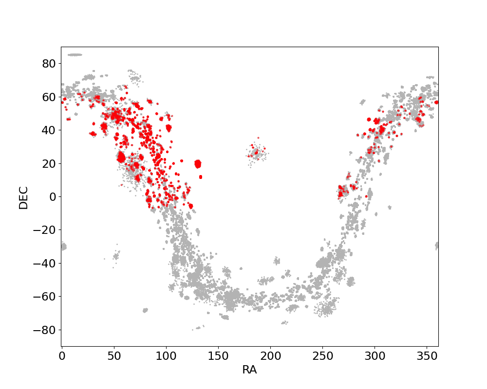
Figure 1: The sky coverage of the LAMOST open cluster (OC) members (red dots) and all the Cantat-Gaudin et al. (2020) OC member stars (grey dots).

To provide accurate chemical and kinematical information for these selected LAMOST OCs, we perform quality control on radial velocity and stellar parameters, respectively.

2.1 Radial velocity quality control

The greatest advantage of LAMOST is the vast number of spectra, but the low resolution makes the stellar RV uncertainty not negligible compared to studies with high-resolution spectra. The median value of the RV uncertainty for our matched LAMOST OC member stars is 6.36$\pm$3.20 km s^-1, which is comparable to or even larger than the typical RV dispersion of a cluster. For instance, the RV dispersion of clusters NGC 2516, NGC 6705, and NGC 6633 are 1.0, 1.6, and 1.5 km s^-1, respectively, as reported in the $Gaia$ -ESO survey based on high resolution spectra (see e.g. Magrini et al., 2017),.

To derive the average RV of clusters, the RV dispersion of each cluster, and a proper RV member quality control, we apply a Monte Carlo (MC) method, by considering each individual RV and its corresponding uncertainty from the LAMOST DR8 catalogue. For simplicity we assume that all RV uncertainties follow Gaussian distributions and then we randomly sample RV of every member star in each cluster 5,000 times. This allows us to derive the mean and median of all the sampled RV values. Member star with RV measurements within 2 $\sigma$ of the MC RV sampling are marked with a quality control flag of flag = 1, while those with $>$ 2 $\sigma$ are marked as flag = 0. The mark of flag = 1 means we use the RV values of the star to determine the cluster radial velocity.

Fig. 2 shows an example of the RV quality control in cluster NGC 2548, where RV of all matched stars are plotted as Gaussian profiles. Dark-grey curves show selected RV member (flag =1), while light-grey curves are stars we discard (flag=0) for the cluster radial velocity determination. The thick blue curve is the Gaussian fit of all the stars with flag=1 in this cluster. The thick blue vertical line represents the mean radial velocity of the cluster ($V_{\rm rad,mean}$). The two vertical dashed lines mark the 2-$\sigma$ departure from $V_{\rm rad,mean}$, which are adopted as thresholds of flag=1 star selections. In the top left region of the Fig. 2, we show numbers of total matched stars in the cluster ($N_{\rm star}$), numbers of RV-selected (flag=1) stars ($N_{\rm star,RV}$), the cluster mean radial velocity ($V_{\rm rad,mean}$), and the corresponding standard deviation ($\sigma\,V_{\rm rad}$), which is adopted as the cluster radial velocity uncertainty, respectively. In most clusters, $V_{\rm rad,mean}$ and the median radial velocity of the cluster $V_{\rm rad,med}$ are very similar to each other, with a mean absolute difference of $\sim$ 0.85 km s^-1. Indeed, 76% of clusters have a difference smaller than this mean value. In the following part of this paper, we use $V_{\rm rad,med}$ to discuss the property of cluster radial velocity $V_{\rm rad}$.

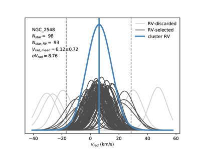
Figure 2: NGC 2548 as an example of the RV selection. The RVs of all the crossed-matched member stars in the cluster are plotted assuming a normal distribution. The light grey colour curves denote stars we discard for further analysis (flag = 0), while the dark grey ones are the selected stars. The two vertical dashed lines mark the 2-$\sigma$ selection criterion. The Monte Carlo model result of all the selected stars is illustrated with the blue Gaussian curve. Their mean RV value ($V_{\rm rad,mean}$), the 1-$\sigma$ RV dispersion ($\sigma V_{\rm rad}$), as well as the number of member stars before ($N_{\rm star}$) and after the RV selection ($N_{\rm star,RV}$), are shown in the legend.

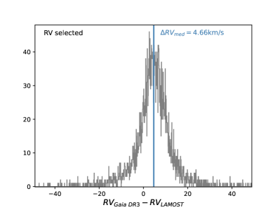
Figure 3: Histogram of the radial velocity difference between $Gaia$ DR3 measurements and LAMOST measurements for all the RV selected members. The median value of the difference $\Delta RV$ = RV${}_{Gaia\leavevmode\nobreak\ DR3}$ - RV_LAMOST is 4.66 km s^-1.

Stellar RV measurements of LAMOST are known to have a systematic offset compared to higher resolution data, with a value about 4-5 km s^-1. In the “Survey of Surveys” work by Tsantaki et al. (2022), where they compare RV measurements from different survey data, the median and mean difference between $Gaia$ DR2 and LAMOST DR5 (RV${}_{Gaia\leavevmode\nobreak\ DR2}$-R_LAMOST) are 4.97 and 5.18 km s^-1, respectively. In Fig. 3 we show the RV measurement difference ($\Delta$RV = RV${}_{Gaia\leavevmode\nobreak\ DR3}$-R_LAMOST) distribution of all the flag=1 OC members. The $\Delta$RV have a median value of 4.66 km s^-1, mean value of 4.82 km s^-1, and a standard deviation of 12.29 km s^-1. All these values based on cluster member stars after the RV quality control are similar to the raw ones reported by Tsantaki et al. (2022) before their RV correction.

2.2 Stellar parameter quality control

Similar to the quality control of $V_{\rm rad}$ described in Sec. 2.1, it is also necessary to control the qualities of stellar parameters before further analysis. This control procedure is based on not only finding [Fe/H] outliers, but also checking member star evolution. In principle, the surface gravity $\log(g)$ and effective temperature $T_{\mathrm{eff}}$ of member stars in the same cluster should follow the evolution of a simple stellar population in the Kiel diagram, where the stellar $\log(g)$ value is an index of the evolutionary phase. The [Fe/H] of these stars, on the other hand, should be almost a constant in different evolutionary phases .

Therefore, such quality control could serve as useful examinations, or even calibrations, to check the accuracy of stellar parameter analysis. In these quality control process to our LAMOST OC member stars, we find a systematic issue for the $\log(g)$ and [Fe/H] parameters of cool main sequence stars. Fig. 4 presents cluster NGC 2632 as an example of such an issue. We find that main sequence stars with $T_{\mathrm{eff}}$ $\lessapprox$ 5000 K do not follow the main sequence evolution trend. For reference, a theoretical isochrone from PARSEC v1.2S (Bressan et al., 2012; Chen et al., 2014, 2015; Tang et al., 2014) with a metallicity of Z=0.013 and log(age)=9.3 is plotted in the Kiel diagram (the upper panel of Fig.4). Most of these stars have a $\log(g)$ value lower than the expected values (see stars in the grey part of the upper panel of Fig. 4). Their [Fe/H] values are also abnormally lower than that of other member stars (see the lower panel of Fig. 4).

On the other hand, giant stars in this temperature regime seem not affected. Member stars’ [Fe/H] values are almost a constant for all giants as well as dwarfs at $T_{\mathrm{eff}}$ $\gtrsim$5000 K. Only the dwarf stars show a decline tend at lower temperature, which is seen in all of our clusters that have dwarf stars in this temperature range. To select OC member stars with a more secure [Fe/H] determination, we discard dwarf stars cooler than 5000 K in our cluster [Fe/H] calculation.

It is always difficult to obtain stellar parameters for very hot and very cool stars. There are few metal lines that can be used in hot star spectra, and the continuum is relatively difficult to derive. For stars with cool temperature, molecular lines dominate their spectra and make the analysis challenging (see discussions in Jofré et al., 2019). Therefore, the second step of our stellar parameter quality control process is excluding [Fe/H] of member stars with $T_{\mathrm{eff}}$ $>$7500 K and $T_{\mathrm{eff}}$ $<$4000 K for the cluster metallicity determinations. The hot star criterion $T_{\mathrm{eff}}$ =7500 K is adopted from LAMOST hot star stellar parameter work (Xiang et al., 2021).

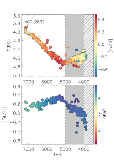
Figure 4: Kiel diagram (upper panel, colour-coded with [Fe/H] ) and [Fe/H] as a function of $T_{\mathrm{eff}}$ (lower panel, colour-coded with $\log(g)$ ) of cluster NGC 2632. For reference, a PARSEC theoretical isochrone of Z=0.013, log(age)=9.3 is plotted in the Kiel diagram. The line-shaded region marks $T_{\mathrm{eff}}$ ¡ 4000 K, and the grey part are 5000 K¡$T_{\mathrm{eff}}$ ¡4000 K.

After the two-step quality control process described above, we end up with 355 OCs for further cluster [Fe/H] determination. The selected member stars are marked with flag=12 in our output catalogue, which means the parameters of these stars are good for both RV and [Fe/H] determination of the cluster. Among these clusters, 203 ones have at least three members with flag=12.

We then calculate the cluster [Fe/H] together with the corresponding uncertainty and scatter using a Monte Carlo method. The mean stellar [Fe/H] uncertainty of our OC member stars from the pipeline LASP is 0.07 dex. Assuming [Fe/H] uncertainty of member stars follow Gaussian distributions, we apply a random [Fe/H] sampling of 5,000 times to each cluster, and obtain the median [Fe/H] _med, mean [Fe/H] _mean, and standard deviation $\sigma$[Fe/H] of all the sample values. The absolute difference between the cluster median [Fe/H] _med and mean [Fe/H] _mean values are very small, with a mean difference of $\sim$0.01 dex. About 70% of clusters have difference smaller than this value. In the rest of this paper, we adopt the median value [Fe/H] _med to discuss the cluster [Fe/H] , and take the sample standard deviation $\sigma$[Fe/H] as the cluster [Fe/H] uncertainty.

Fig. 5 shows the CMD of member stars with $Gaia$ DR2 photometry of two very typical OCs in our catalogue. They are Melotte 22 (Pleiades) in the upper two panels and NGC 2682 (M67) in the lower two panels. The left panel of each cluster is colour-coded with member star [Fe/H] , which means all the coloured ones are flag=12 stars. The right panel of each cluster is colour-coded with member star RV, marking all the flag=1 stars in the cluster. The derived cluster $V_{\rm rad}$ and [Fe/H] values based on the flag=1 and flag=12 members, respectively, are shown in the figure.

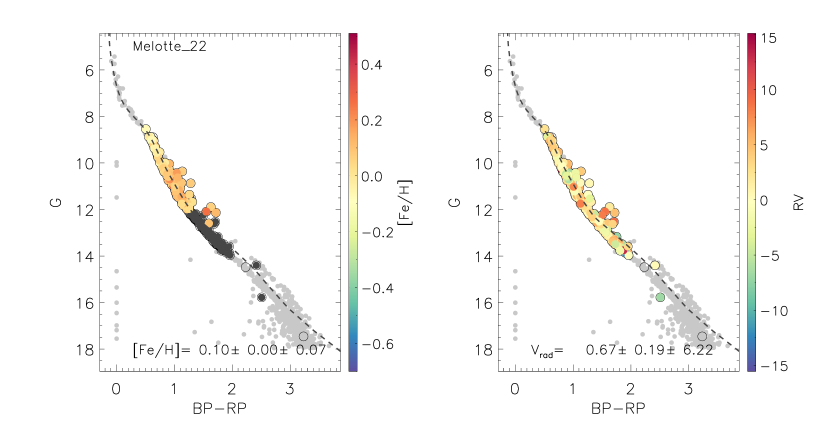
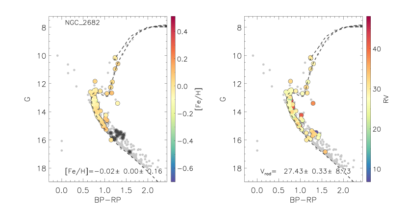
Figure 5: Colour-magnitude diagrams of Melotte 22 and NGC 2682 as examples of the clusters with [Fe/H] in the literature. The grey filled circles are high quality member stars from Cantat-Gaudin et al. (2020), and open circles are all matched stars with LAMOST RV measurements. In the right panel stars good for the cluster $V_{\rm rad}$ determination (flag=1) are colour-coded with their RV values. In the left panel, the colour-filled dots are stars good for [Fe/H] determination (flag=12), and the black ones are stars without [Fe/H] determination or with discarded [Fe/H] . The dashed curve in each sub-figure is the PARSEC isochrone with the Cantat-Gaudin et al. (2020) cluster parameters.

3 Results

3.1 Radial Velocity

3.1.1 Clusters with V_rad in the literature

Catalogues of the Galactic OC radial velocity have been compiled in many works (see e.g. Dias et al., 2002; Kharchenko et al., 2013; Conrad et al., 2014; Soubiran et al., 2018; Dias et al., 2021; Tarricq et al., 2021). We compare our cluster V_rad results to the two most recent and most complete large catalogues, from Tarricq et al. (2021) and Dias et al. (2021), together with the previous LAMOST OC catalogue from Zhong et al. (2020).

Among all our 386 OCs, we found 308 in common with Tarricq et al. (2021), 185 in common with Dias et al. (2021), and 226 in common with Zhong et al. (2020). Figure 6 shows the comparison of the cluster $V_{\rm rad}$ between our results and these three catalogues. The distributions of the $V_{\rm rad}$ difference are also displayed as a histogram in each panel. Compared to the previous LAMOST OC results from Zhong et al. (2020), the median value of the $V_{\rm rad}$ difference is only 0.06 km s^-1(see the right panel of Fig. 6 ), which indicates that the two catalogues are consistent in $V_{\rm rad}$. The median $V_{\rm rad}$ difference between our results and the ones from Tarricq et al. (2021) and Dias et al. (2021) have a value around 6.2 km s^-1 (see the left and middle panel of Fig. 6). These differences should, at least partially, be due to the aforementioned systematic offset of LAMOST RV.

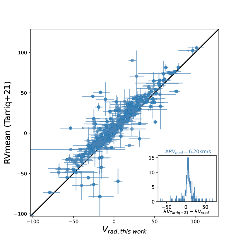
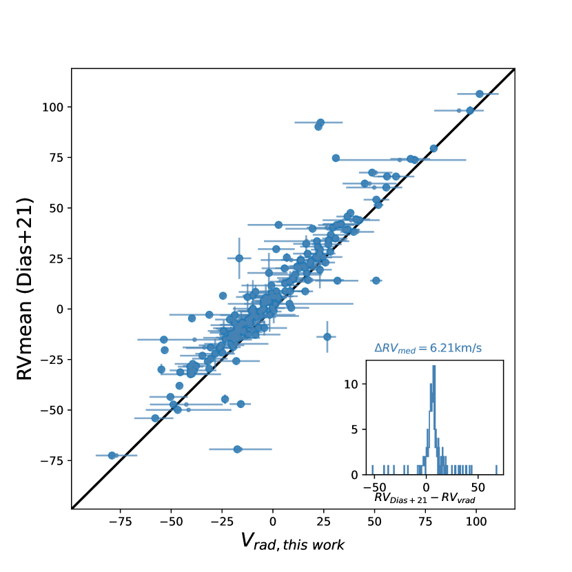
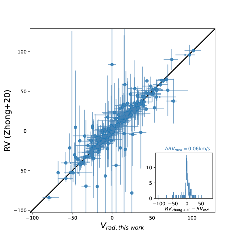
Figure 6: Comparison of our cluster $V_{\rm rad}$ to results in the literature. The left, middle, and right panels show comparison to 308, 185, and 226 OCs of Tarricq et al. (2021), Dias et al. (2021), and Zhong et al. (2020), respectively. The histograms of the cluster radial velocity differences are shown as insets in each panel.

In total, 342 of the OCs in our catalogue already have a $V_{\rm rad}$ measurement in one of these three recent large catalogues. Their $V_{\rm rad}$, $\sigma\,V_{\rm rad}$, number of stars used in the calculation, together with the literature values, are listed in Table 1.

Table 1: Radial velocity of 342 OCs with known $V_{\rm rad}$ in the literature.

cluster	Nall	Nflag1	Vrad,med	Vrad,mean	$\sigma$Vrad	RVTarricq21	NRV	RVDias21	NRV	RVZhong20	NRV
ASCC_10	23	22	-24.20 $\pm$ 1.57	-24.58 $\pm$ 1.23	7.42	-15.61 $\pm$ 4.35	3	-10.87 $\pm$ 5.24	3	-27.21 $\pm$ 5.91	33
ASCC_11	39	39	-21.37 $\pm$ 1.94	-21.02 $\pm$ 1.51	13.18	-14.44 $\pm$ 0.32	3	-14.24 $\pm$ 0.23	3	-21.49 $\pm$ 12.74	52
ASCC_105	5	5	-18.98 $\pm$ 3.05	-18.47 $\pm$ 3.16	5.95	-6.93 $\pm$ 1.36	19	-14.30 $\pm$ 4.09	18	-20.01 $\pm$ 2.47	6
ASCC_108	11	11	-14.93 $\pm$ 3.69	-14.75 $\pm$ 3.41	10.84	-29.67 $\pm$ 19.60	2			-14.73 $\pm$ 6.22	12
…	…	…	…	…	…	…	…	…	…	…

3.1.2 Clusters with newly-obtained $V_{\rm rad}$

The large number of LAMOST spectra enables us to obtain cluster $V_{\rm rad}$ values that were not reported in the literature before. We report here 44 clusters with newly-obtained $V_{\rm rad}$. Table 2 lists their information. These values, together with those listed in Table 1, will be employed later in the paper, for a kinematical analysis of the OC population.

Table 2: Newly-obtained cluster radial velocity of 44 OCs.

cluster	Nall	Nflag1	Vrad,med	Vrad,mean	$\sigma$Vrad
COIN-Gaia_24	44	44	-9.20 $\pm$ 1.35	-9.20 $\pm$ 1.16	8.22
LP_2139	36	34	-4.34 $\pm$ 2.06	-4.03 $\pm$ 1.67	11.62
UBC_88	29	28	-15.78 $\pm$ 2.12	-16.76 $\pm$ 1.71	12.11
COIN-Gaia_23	18	17	1.72 $\pm$ 3.44	1.35 $\pm$ 2.71	12.55
COIN-Gaia_19	17	17	8.53 $\pm$ 2.70	8.81 $\pm$ 2.75	12.64
UBC_616	13	13	52.19 $\pm$ 3.56	50.51 $\pm$ 2.53	14.18
COIN-Gaia_17	13	12	6.80 $\pm$ 2.97	6.84 $\pm$ 2.38	8.94
UPK_282	11	11	-16.46 $\pm$ 2.39	-16.80 $\pm$ 1.92	7.94
UBC_51	9	9	-14.65 $\pm$ 4.73	-19.19 $\pm$ 3.48	17.67
UBC_56	8	8	-12.43 $\pm$ 4.44	-11.97 $\pm$ 3.87	10.75
COIN-Gaia_14	8	8	4.56 $\pm$ 3.46	5.17 $\pm$ 2.66	10.80
COIN-Gaia_39	7	7	-3.84 $\pm$ 4.86	-0.49 $\pm$ 3.70	15.47
UPK_119	5	5	-24.34 $\pm$ 3.16	-24.37 $\pm$ 2.55	5.30
UBC_63	5	5	-22.94 $\pm$ 4.49	-22.15 $\pm$ 3.50	8.99
UBC_80	4	4	38.54 $\pm$ 8.40	38.92 $\pm$ 7.91	13.37
UBC_615	4	4	13.47 $\pm$ 8.18	13.32 $\pm$ 5.87	25.94
COIN-Gaia_20	4	4	-4.35 $\pm$ 5.00	-4.97 $\pm$ 5.06	8.66
UBC_201	4	4	19.08 $\pm$ 6.98	19.52 $\pm$ 6.14	12.94
UBC_188	4	4	-35.56 $\pm$ 6.49	-36.03 $\pm$ 7.86	12.79
UPK_312	4	4	-12.03 $\pm$ 4.01	-11.75 $\pm$ 3.79	6.72
UBC_77	3	3	17.30 $\pm$ 5.95	17.67 $\pm$ 5.26	7.00
UBC_68	3	3	13.19 $\pm$ 5.87	13.06 $\pm$ 4.78	7.31
NGC_381	3	3	-22.88 $\pm$ 6.32	-22.93 $\pm$ 5.57	7.06
COIN-Gaia_40	3	3	7.47 $\pm$ 7.92	8.42 $\pm$ 7.08	11.55
UBC_437	3	3	19.37 $\pm$ 10.24	18.60 $\pm$ 7.24	15.07
UBC_417	3	3	-47.45 $\pm$ 7.35	-47.74 $\pm$ 4.63	9.88
NGC_2169	3	3	14.32 $\pm$ 4.22	14.47 $\pm$ 3.67	4.93
SAI_14	2	2	-69.73 $\pm$ 3.00	-69.73 $\pm$ 3.00	2.51
UBC_198	2	2	-7.13 $\pm$ 7.70	-7.13 $\pm$ 7.70	7.18
UBC_129	2	2	-17.90 $\pm$ 7.33	-17.90 $\pm$ 7.33	6.08
UBC_216	1	1	-1.11 $\pm$ 10.05
UBC_395	1	1	-13.62 $\pm$ 17.02
UBC_150	1	1	-17.43 $\pm$ 6.96
Teutsch_8	1	1	-17.62 $\pm$ 6.45
UPK_131	1	1	-20.25 $\pm$ 5.84
UBC_182	1	1	-28.86 $\pm$ 5.37
UBC_596	1	1	-29.18 $\pm$ 15.03
UBC_430	1	1	-33.62 $\pm$ 12.74
UBC_421	1	1	-40.23 $\pm$ 13.84
UBC_214	1	1	42.81 $\pm$ 11.46
UBC_442	1	1	30.82 $\pm$ 5.93
UBC_206	1	1	27.55 $\pm$ 10.13
COIN-Gaia_21	1	1	1.41 $\pm$ 10.77
UBC_435	1	1	-0.68 $\pm$ 13.71

3.2 Metallicity

As groups of stars form together with the same composition, OCs are an ideal probe to trace the metallicity evolution of the Galactic disc. With OCs, in fact, not only we can improve the S/N by averaging over several member stars, but also we could deal with objects whose age can be determined with a lower uncertainty than that of field stars (with the only possible exception of stars for which a full asteroseismologic analysis is possible, see e.g. Rodrigues et al. (2017); Miglio et al. (2021) ).

In this section we report the metallicity of LAMOST OCs, which consists of 218 clusters with known metallicity collected from the literature, and 137 clusters with newly-obtained spectroscopic metallicity. Here we use the iron abundance [Fe/H] as an index of the stellar metallicity.

3.2.1 Clusters with [Fe/H] in the literature

We collect cluster [Fe/H] measurements from high resolution (HRS) spectra including results of large surveys such as $Gaia$-ESO (Spina et al., 2017; Bragaglia et al., 2022; Randich et al., 2022, and references therein), APOGEE (Donor et al., 2020; Carrera et al., 2019; Spina et al., 2021), GALAH (Carrera et al., 2019; Spina et al., 2021), large projects like SPA (Origlia et al., 2019; Casali et al., 2020a; Zhang et al., 2021; Alonso-Santiago et al., 2021), OCCASO (Casamiquela et al., 2016, 2017, 2018), and high quality (HQ) collections from Netopil et al. (2022). In general, the HRS spectra results we use are similar to the one used in Zhang et al. (2021), but with more OCs from Spina et al. (2021) and HQ results of Netopil et al. (2022). In total, we have 82 clusters in common with HRS [Fe/H] results. The left panel of Fig. 7 shows the comparison between our results based on LAMOST and the HRS values. The difference between the cluster [Fe/H] values of these two data sets, is 0.01$\pm$0.15 dex.

Clusters with less than three member stars for the [Fe/H] determination, both in our case (marked with open square of Fig. 7) and in the HRS works (marked with X), show a relatively large difference between the two sets of result. If we compare clusters with at least three [Fe/H] member stars in both datasets, their difference is 0.00$\pm$0.11 dex, which shows a very good consistency. Therefore, in the following discussions on the Galactic metallicity evolution we only consider clusters with at least three members and with flag=12.

We also compare our results to the previous LAMOST OC work by Zhong et al. (2020) which is based on an earlier data release and different member star selection. There are 206 clusters in the Zhong et al. (2020) catalogue with [Fe/H] determination, the right panel of Fig. 7 shows the [Fe/H] comparison. For all the matched clusters, the [Fe/H] value mean difference is 0.02$\pm$0.23 dex. When only clusters with at least three [Fe/H] member stars are considered, their difference is 0.04$\pm$0.06 dex.

Combining both literature results from HRS studies and low resolution spectra study of Zhong et al. (2020), 218 of our clusters have a reported metallicity. Table 3 lists their information.

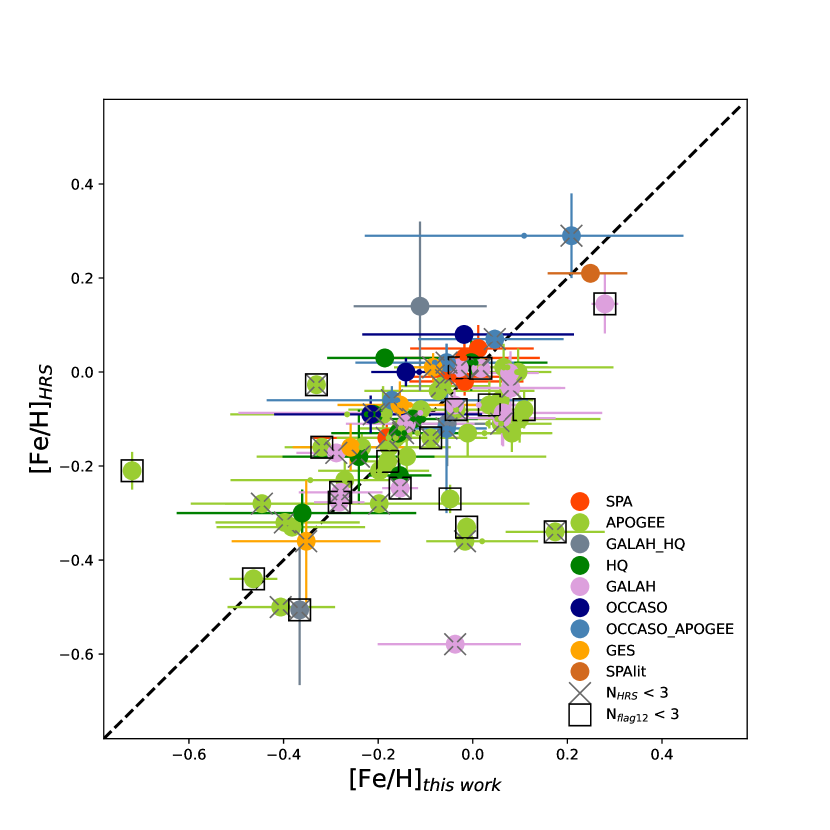
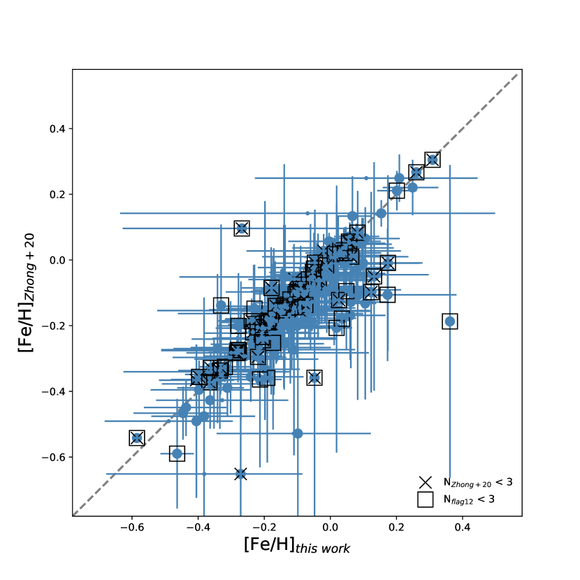
Figure 7: Comparison of 82 clusters’ [Fe/H] to literature results with high resolution spectra (HRS) in the left panel, and of 206 clusters to results from Zhong et al. (2020). The symbol X marks [Fe/H] values with less than 3 member stars, namely 38 clusters on the left (from HRS) and 75 clusters on the right (from Zhong et al., 2020). The open square marks clusters with less than three flag=12 member stars from this work, which are 23 clusters on the left panel and 92 clusters on the right panel.

Table 3: 218 clusters with [Fe/H] values in literature.

cluster	Nflag=12	[Fe/H]med	[Fe/H]mean	$\sigma$[Fe/H]	[Fe/H]HRS	NHRS	source	[Fe/H]Zhong20	NZhong20
ASCC_10	12	-0.03 $\pm$ 0.01	-0.02 $\pm$ 0.01	0.06				-0.10 $\pm$ 0.10	22
ASCC_11	28	-0.18 $\pm$ 0.03	-0.16 $\pm$ 0.03	0.18	-0.14 $\pm$ 0.05	1	SPA	-0.24 $\pm$ 0.09	26
…	…	…	…	…	…	…	…	…	…

3.2.2 Clusters with newly-obtained [Fe/H] 

Here we report [Fe/H] measurements of 137 OCs which do not have spectroscopic [Fe/H] in the literature. Among them, 63 clusters have at least three flag=12 member stars. Table 4 and table 5 list our results for these clusters. Clusters with less than three flag=12 member stars are available in our final catalog as well, but their metallicities should be used with caution. This constitutes an important addition to the number of OCs with metallicity determined on the basis of spectroscopy.

Table 4: Newly-obtained iron abundances for 63 OCs with at least three flag=12 member stars.

cluster	Nflag12	[Fe/H]med	[Fe/H]mean	$\sigma$[Fe/H]	cluster	Nflag12	[Fe/H]med	[Fe/H]mean	$\sigma$[Fe/H]
COIN-Gaia_9	4	0.01 $\pm$ 0.03	-0.01 $\pm$ 0.02	0.09	UBC_6	4	-0.01 $\pm$ 0.02	0.00 $\pm$ 0.02	0.06
COIN-Gaia_10	3	-0.06 $\pm$ 0.11	-0.08 $\pm$ 0.09	0.16	UBC_8	38	-0.12 $\pm$ 0.02	-0.12 $\pm$ 0.01	0.12
COIN-Gaia_11	23	0.16 $\pm$ 0.03	0.16 $\pm$ 0.02	0.18	UBC_51	3	0.04 $\pm$ 0.02	0.05 $\pm$ 0.03	0.03
COIN-Gaia_12	7	-0.00 $\pm$ 0.03	-0.03 $\pm$ 0.05	0.14	UBC_53	4	-0.04 $\pm$ 0.04	-0.04 $\pm$ 0.03	0.07
COIN-Gaia_13	30	-0.07 $\pm$ 0.01	-0.05 $\pm$ 0.02	0.13	UBC_54	37	-0.08 $\pm$ 0.02	-0.08 $\pm$ 0.02	0.16
COIN-Gaia_14	6	0.01 $\pm$ 0.08	0.01 $\pm$ 0.07	0.17	UBC_55	11	-0.12 $\pm$ 0.03	-0.11 $\pm$ 0.03	0.12
COIN-Gaia_17	11	-0.07 $\pm$ 0.05	-0.02 $\pm$ 0.03	0.18	UBC_56	3	-0.05 $\pm$ 0.11	-0.02 $\pm$ 0.11	0.17
COIN-Gaia_18	17	-0.07 $\pm$ 0.03	-0.08 $\pm$ 0.03	0.16	UBC_59	3	-0.11 $\pm$ 0.04	-0.13 $\pm$ 0.08	0.10
COIN-Gaia_19	12	-0.06 $\pm$ 0.03	-0.09 $\pm$ 0.04	0.15	UBC_63	3	-0.12 $\pm$ 0.08	-0.13 $\pm$ 0.08	0.11
COIN-Gaia_20	3	-0.06 $\pm$ 0.04	-0.06 $\pm$ 0.02	0.05	UBC_74	33	-0.10 $\pm$ 0.01	-0.09 $\pm$ 0.02	0.10
COIN-Gaia_23	12	-0.16 $\pm$ 0.05	-0.14 $\pm$ 0.06	0.21	UBC_77	3	-0.04 $\pm$ 0.04	-0.05 $\pm$ 0.05	0.06
COIN-Gaia_24	42	0.06 $\pm$ 0.01	0.01 $\pm$ 0.01	0.13	UBC_88	20	-0.02 $\pm$ 0.02	-0.04 $\pm$ 0.02	0.13
COIN-Gaia_26	9	-0.13 $\pm$ 0.04	-0.11 $\pm$ 0.04	0.21	UBC_434	3	-0.46 $\pm$ 0.07	-0.47 $\pm$ 0.06	0.08
COIN-Gaia_27	3	-0.03 $\pm$ 0.08	-0.03 $\pm$ 0.08	0.10	UBC_586	3	0.08 $\pm$ 0.07	0.08 $\pm$ 0.05	0.08
COIN-Gaia_28	3	-0.14 $\pm$ 0.05	-0.13 $\pm$ 0.06	0.07	UBC_609	3	-0.11 $\pm$ 0.09	-0.12 $\pm$ 0.07	0.13
COIN-Gaia_38	5	0.02 $\pm$ 0.10	0.03 $\pm$ 0.07	0.19	UBC_614	3	-0.01 $\pm$ 0.11	-0.00 $\pm$ 0.07	0.14
COIN-Gaia_39	3	-0.08 $\pm$ 0.10	-0.04 $\pm$ 0.10	0.17	UBC_615	4	-0.15 $\pm$ 0.14	-0.15 $\pm$ 0.11	0.23
COIN-Gaia_41	5	-0.14 $\pm$ 0.07	-0.14 $\pm$ 0.07	0.17	UBC_616	4	-0.25 $\pm$ 0.04	-0.28 $\pm$ 0.05	0.14
LP_2139	30	-0.19 $\pm$ 0.03	-0.17 $\pm$ 0.03	0.19	UBC_619	5	-0.18 $\pm$ 0.06	-0.17 $\pm$ 0.08	0.15
NGC_381	3	-0.13 $\pm$ 0.05	-0.10 $\pm$ 0.03	0.10	UBC_622	3	-0.15 $\pm$ 0.03	-0.15 $\pm$ 0.02	0.05
NGC_1502	5	0.04 $\pm$ 0.06	0.03 $\pm$ 0.04	0.10	UPK_119	5	0.03 $\pm$ 0.02	0.03 $\pm$ 0.02	0.08
NGC_2126	21	-0.23 $\pm$ 0.02	-0.21 $\pm$ 0.03	0.17	UPK_166	7	0.02 $\pm$ 0.03	-0.07 $\pm$ 0.08	0.26
NGC_6997	3	0.07 $\pm$ 0.04	0.06 $\pm$ 0.05	0.06	UPK_168	4	0.10 $\pm$ 0.02	0.07 $\pm$ 0.05	0.10
UBC_2	7	-0.05 $\pm$ 0.04	-0.04 $\pm$ 0.05	0.12	UPK_185	10	0.01 $\pm$ 0.01	0.01 $\pm$ 0.01	0.04
UBC_4	14	-0.11 $\pm$ 0.02	-0.08 $\pm$ 0.01	0.15	UPK_282	7	-0.05 $\pm$ 0.03	-0.06 $\pm$ 0.03	0.08
UBC_13	19	-0.07 $\pm$ 0.03	-0.05 $\pm$ 0.03	0.13	UPK_294	3	-0.16 $\pm$ 0.07	-0.15 $\pm$ 0.06	0.09
UBC_19	7	0.09 $\pm$ 0.01	0.08 $\pm$ 0.05	0.10	UPK_296	16	-0.05 $\pm$ 0.01	-0.03 $\pm$ 0.02	0.14
UBC_31	23	-0.01 $\pm$ 0.01	0.00 $\pm$ 0.01	0.08	UPK_305	12	0.05 $\pm$ 0.02	0.05 $\pm$ 0.01	0.07
UBC_188	3	0.02 $\pm$ 0.04	-0.17 $\pm$ 0.05	0.31	UPK_350	13	-0.06 $\pm$ 0.03	-0.04 $\pm$ 0.03	0.12
UBC_200	17	-0.21 $\pm$ 0.03	-0.16 $\pm$ 0.03	0.21	UPK_381	8	-0.04 $\pm$ 0.08	-0.04 $\pm$ 0.06	0.18
UBC_203	6	-0.39 $\pm$ 0.05	-0.37 $\pm$ 0.03	0.14	UPK_429	9	0.01 $\pm$ 0.05	0.02 $\pm$ 0.07	0.19
UBC_433	3	-0.52 $\pm$ 0.13	-0.52 $\pm$ 0.10	0.17

Table 5: Newly-obtained iron abundances for 74 OCs but with less than three flag=12 member stars.

cluster	Nflag12	[Fe/H]med	[Fe/H]mean	$\sigma$[Fe/H]	cluster	Nflag12	[Fe/H]med	[Fe/H]mean	$\sigma$[Fe/H]
Berkeley_34	2	-0.21 $\pm$ 0.06	-0.21 $\pm$ 0.06	0.05	UBC_216	1	-0.07 $\pm$ 0.12
COIN-Gaia_2	1	-0.24 $\pm$ 0.21			UBC_374	2	0.19 $\pm$ 0.03	0.19 $\pm$ 0.03	0.03
COIN-Gaia_8	2	-0.05 $\pm$ 0.04	-0.05 $\pm$ 0.04	0.08	UBC_395	1	-0.06 $\pm$ 0.09
COIN-Gaia_15	1	-0.01 $\pm$ 0.09			UBC_417	2	-0.04 $\pm$ 0.02	-0.04 $\pm$ 0.02	0.05
COIN-Gaia_16	1	-0.12 $\pm$ 0.08			UBC_419	1	-0.09 $\pm$ 0.06
COIN-Gaia_21	1	-0.11 $\pm$ 0.19			UBC_421	1	-0.37 $\pm$ 0.19
COIN-Gaia_22	1	-0.26 $\pm$ 0.26			UBC_427	1	0.20 $\pm$ 0.06
Collinder_115	1	-0.17 $\pm$ 0.19			UBC_428	2	-0.35 $\pm$ 0.16	-0.35 $\pm$ 0.16	0.13
Collinder_421	2	-0.02 $\pm$ 0.04	-0.02 $\pm$ 0.04	0.04	UBC_430	1	-0.45 $\pm$ 0.13
Czernik_38	1	0.54 $\pm$ 0.10			UBC_431	1	-0.47 $\pm$ 0.15
Dolidze_5	1	-1.93 $\pm$ 0.16			UBC_436	2	-0.19 $\pm$ 0.04	-0.19 $\pm$ 0.04	0.03
FSR_0932	1	-2.17 $\pm$ 0.06			UBC_437	2	-0.20 $\pm$ 0.14	-0.20 $\pm$ 0.14	0.12
FSR_0975	1	-0.18 $\pm$ 0.22			UBC_438	1	-0.39 $\pm$ 0.06
LP_658	1	-0.32 $\pm$ 0.08	-0.32 $\pm$ 0.08	0.00	UBC_440	2	-0.26 $\pm$ 0.05	-0.26 $\pm$ 0.05	0.10
LP_930	1	0.16 $\pm$ 0.04			UBC_442	1	-0.08 $\pm$ 0.06
LP_2198	2	0.25 $\pm$ 0.15	0.25 $\pm$ 0.15	0.13	UBC_445	1	-0.04 $\pm$ 0.33
NGC_457	1	-0.14 $\pm$ 0.18			UBC_587	1	-0.22 $\pm$ 0.08
NGC_2169	1	-0.05 $\pm$ 0.04			UBC_596	1	-0.19 $\pm$ 0.07
NGC_6871	1	0.26 $\pm$ 0.03			UBC_607	2	-0.38 $\pm$ 0.09	-0.38 $\pm$ 0.09	0.12
SAI_14	2	-0.41 $\pm$ 0.08	-0.41 $\pm$ 0.08	0.07	UBC_610	2	-0.26 $\pm$ 0.06	-0.26 $\pm$ 0.06	0.23
Sigma_Ori	2	-0.46 $\pm$ 0.06	-0.46 $\pm$ 0.06	0.22	UBC_629	2	-0.38 $\pm$ 0.06	-0.38 $\pm$ 0.06	0.04
Teutsch_8	1	0.11 $\pm$ 0.18			UPK_45	2	0.08 $\pm$ 0.06	0.08 $\pm$ 0.06	0.05
Teutsch_35	2	0.12 $\pm$ 0.03	0.12 $\pm$ 0.03	0.03	UPK_65	1	0.02 $\pm$ 0.13
UBC_49	2	-0.18 $\pm$ 0.06	-0.18 $\pm$ 0.06	0.08	UPK_79	2	-0.04 $\pm$ 0.04	-0.04 $\pm$ 0.04	0.04
UBC_52	1	0.04 $\pm$ 0.08			UPK_82	1	0.04 $\pm$ 0.01
UBC_57	2	-0.25 $\pm$ 0.09	-0.25 $\pm$ 0.09	0.07	UPK_93	2	-0.01 $\pm$ 0.01	-0.01 $\pm$ 0.01	0.01
UBC_61	1	0.10 $\pm$ 0.16			UPK_108	2	0.00 $\pm$ 0.02	0.00 $\pm$ 0.02	0.03
UBC_68	2	-0.12 $\pm$ 0.10	-0.12 $\pm$ 0.10	0.09	UPK_131	1	0.02 $\pm$ 0.03
UBC_73	2	-0.19 $\pm$ 0.18	-0.19 $\pm$ 0.18	0.14	UPK_136	2	-0.05 $\pm$ 0.05	-0.05 $\pm$ 0.05	0.14
UBC_82	1	-0.13 $\pm$ 0.03			UPK_303	2	0.12 $\pm$ 0.02	0.12 $\pm$ 0.02	0.02
UBC_90	1	-0.28 $\pm$ 0.15	-0.28 $\pm$ 0.15	0.00	UPK_333	2	-0.05 $\pm$ 0.05	-0.05 $\pm$ 0.05	0.05
UBC_141	2	-0.09 $\pm$ 0.04	-0.09 $\pm$ 0.04	0.03	UPK_369	2	0.18 $\pm$ 0.03	0.18 $\pm$ 0.03	0.20
UBC_150	1	-0.05 $\pm$ 0.01			UPK_379	1	-0.05 $\pm$ 0.03
UBC_169	1	-0.08 $\pm$ 0.02			UPK_385	2	0.13 $\pm$ 0.01	0.13 $\pm$ 0.01	0.04
UBC_176	1	0.12 $\pm$ 0.21			UPK_418	2	-0.25 $\pm$ 0.07	-0.25 $\pm$ 0.07	0.11
UBC_182	1	-0.14 $\pm$ 0.29			UPK_422	1	0.06 $\pm$ 0.06
UBC_197	1	-0.08 $\pm$ 0.03			vdBergh_85	1	-0.24 $\pm$ 0.11

4 Discussions

4.1 The Galactic metallicity distribution and dynamical properties of the LAMOST OCs

In order to study the metallicity distribution of the Milky Way disc, one of the most common subjects investigated is the so-called radial metallicity gradient. The metallicity gradient is often displayed with [Fe/H] as a function of the Galactocentric radius $R_{\rm GC}$ , indicating different levels of metal enrichment along the Galactic radius. Stellar open clusters, being groups of stars in a simple stellar population, are ideal probes to trace the metal enrichment history of the Milky Way.

With the homogeneous V_rad and [Fe/H] determination in our newly compiled LAMOST OC catalogue, we can investigate the evolution of the Galactic metallicity – even its gradient evolution – in the past 500 Myr. This 500-Myr range traces back to the time when the Sagittarius dwarf galaxy (Sgr dSph) had its last passage through the MW outer disc (see for instance the discussions in Xu et al., 2020). Sgr dSph is also the last relatively considerable minor merger in the evolution history of our galaxy known to date, which means the gravitational potential of the Galaxy can be considered as a constant in the past 500 Myr. A stable gravitational potential is further the guarantee of orbit calculations for these clusters.

To trace back the orbits of LAMOST OCs and their evolution, we use the publicly licensed code GALPOT (Dehnen & Binney, 1998) and the Milky Way gravitational potential from McMillan (2017). The gravitational potential takes into account the Galactic thick and thin stellar discs, a bulge component, a dark-matter halo, and a cold gas disc. We adopt the Solar motion of (U, V, W)_⊙ = (11.1, 12.24, 7.25) km s^-1 (Schönrich et al., 2010), which is insensitive to the metallicity gradient of the MW disc. The Galactic radius of the Sun is 8.2 kpc, the solar circular speed is 232.8 km s^-1, both suggested by McMillan (2017). Proper motions and distances of clusters are adopted from Cantat-Gaudin et al. (2020).

Figure 8 shows the Galactic metallicity gradient traced by LAMOST OCs in six snapshots during the past 500 Myr, that is, from the present time (look back time 0 Myr, uppermost left panel) back to the time of the last passage of Sgr dSph. It is very difficult for LAMOST to observe stars toward the Galactic centre, so almost all the LAMOST OCs are located with Galactocentric radii $R_{\rm GC}\gtrapprox$8 kpc. As discussed earlier, only clusters with no less than three flag=12 stars are used in the following metallicity discussions. Here we also make a simplification that the cluster [Fe/H] does not change in its life time, i.e., the microscopic diffusion in the stellar surface layer is not considered. To investigate the metal enrichment in different epochs, we divide the LAMOST OCs into six age groups (colour-coded). A second-order polynomial fitting is applied to each age group to measure their metallicity trend:

$$\texttt{[Fe/H]}={a\times R_{GC}^{2}+b\times R_{GC}+c}$$ (1)

For each fitting, we use a Markov chain Monte Carlo (MCMC) method to consider the [Fe/H] uncertainty of each cluster. A number of 300 walkers and an 10,000-step MCMC are used in each fitting, based on the MCMC python package emcee (Foreman-Mackey et al., 2013). The parameters (a, b, c) to second-order polynomial fits of the current time are listed in the $R_{\rm GC}$ column of Table 6.

In the literature, a linear fit has been widely adopted to describe the metallicity radial gradient (see e.g. Friel et al., 2002; Bragaglia & Tosi, 2006; Carrera et al., 2019; Zhong et al., 2020; Zhang et al., 2021), but a break or a “knee” point is needed at $\sim$ 12–14 kpc in order to properly take into account the outer disc clusters (see e.g. Reddy et al., 2016; Donor et al., 2020; Spina et al., 2022). Indeed, radial metallicity distribution studies in other galaxies suggest that breaks and changes of slopes are required in the linear fittings, and non-linear models often fit better than linear models (Scarano & Lépine, 2013). For this reason we use the second-order polynomial model fittings to illustrated the metallicity trends. From the six snapshots of the [Fe/H] trend in Fig. 8, it is clear that, though generally speaking [Fe/H] is higher at smaller $R_{\rm GC}$ , the metallicity gradients evolve among age groups, instead of being a constant curve. In other words, if we were observing OCs at different times in the past 500 Myr, we would have seen very different pictures of the metallicity gradient(s): It covers multiple shapes of being steep, flat, with a turning point, and close to a straight line.

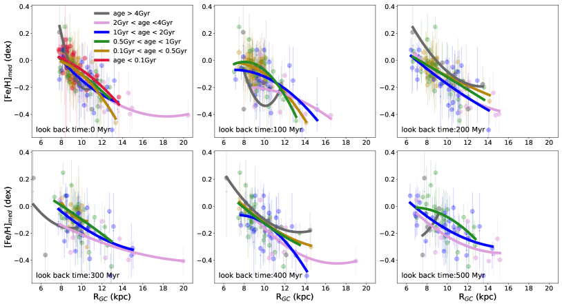
Figure 8: The clusters’ median [Fe/H] as a function of the Galactocentric radius $R_{\rm GC}$ for all the LAMOST clusters with at least three flag=12 stars. Different panels show different look back times according to the orbit calculations. Clusters are divided into six groups according to age from the Cantat-Gaudin et al. (2020) catalogue. The solid curves are the second-order polynomial MCMC fittings of each age group.

In order to interpret radial metallicity gradient variations for different age groups, we modelled the circular orbits of each cluster with GALPOT. Note that radial metallicity gradients are themselves trajectory projections of cluster orbits. We find that the clusters are not travelling in circular orbits. Figure 9 shows the eccentricity (ecc) of LAMOST OCs as a function of their Galactic apocentre distance. Though GALPOT does not give uncertainties of the orbit parameters, we calculate the possible orbit parameter changes according to the scatter of clusters’ V_rad.

Most clusters have a non-circular orbit (ecc$>$0). For instance, Berkeley 29 has at present the highest $R_{\rm GC}$ = 20.44 kpc, being located on the outermost disc in our catalog. However, its apocentric and pericentric distances are 20.54 kpc and 13.92 kpc, respectively, with an eccentricity of 0.19. The most eccentric cluster with at least three flag=12 member stars in our sample is Berkeley 32 (ecc = 0.31). It has a current $R_{\rm GC}$ of 11.00 kpc, but it travels to 12.23 kpc and 6.42 kpc as its apocentre and pericentre, respectively.

Generally speaking, the youngest clusters are more likely to travel with a more circular orbit, while the oldest clusters have higher chances to have larger eccentricity (see the left panel of Fig. 9). The metal-poorer open clusters, whether or not they have a circular orbit, can reach larger apocentric distances than the metal-richer clusters (see the right panel of Fig. 9). The non-circular orbit around the Galactic centre results in clusters that constantly and periodically alter their $R_{\rm GC}$ between their pericentre and apocentre. The alteration period is shorter than one revolution time of the cluster, making the cluster travel back and forth several times in one revolution around the Galactic centre (see also discussions in Lépine et al., 2011). All these facts make the present-day Galactocentric radius $R_{\rm GC}$ not an invariant in the Galactic metallicity distribution investigations.

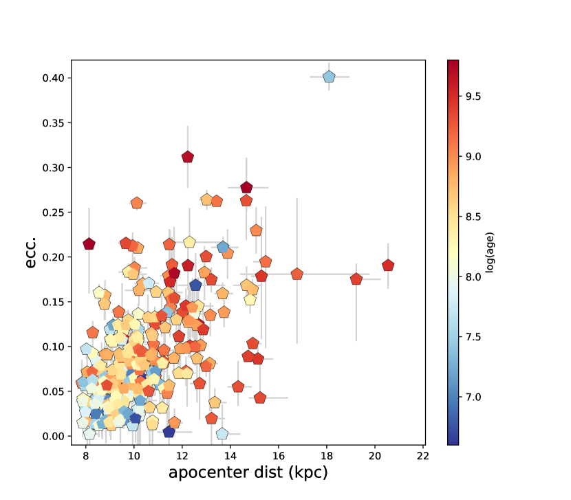
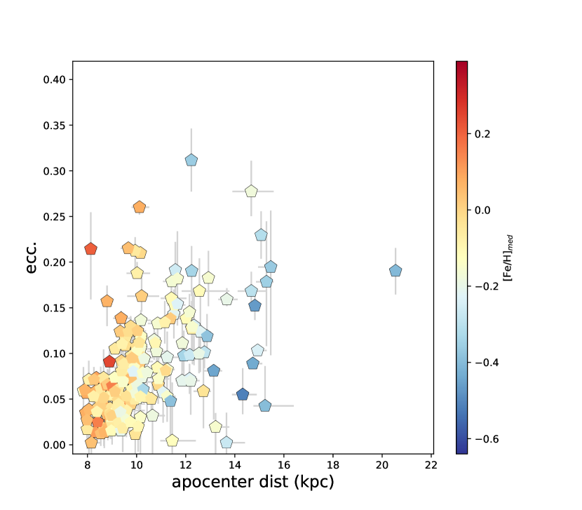
Figure 9: The clusters’ eccentricity as a function of their Galactic apocentric distance. The colour code is the log value of the cluster age in the left panel, and cluster [Fe/H] in the right panel. Only clusters with multiple members are displayed in the left panel, while those with at least three flag=12 stars are displayed in the right panel.

Thanks to the astrometry results provided by $Gaia$ and radial velocity provided by spectroscopic facilities such as LAMOST, we can now use more invariant parameters such as the angular momenta and the dynamical energy to unfold the whole story of the Galactic [Fe/H] evolution in the $Gaia$ era. In Fig. 10 we display the [Fe/H] distribution of the LAMOST OCs as a function of the Z component of their angular momentum (left panel) and the total dynamical energy (right panel). The corresponding uncertainties reflect the scatter of clusters’ V_rad. These two parameters take into account both the spatial positions and the motions, so they are constant for a cluster in a given gravitational potential. We calculate them with GALPOT following the same setups described before in the orbit integration part. The Z component of the angular momentum ($L_{\rm Z}$), i.e. the angular momentum component that describes the motion around the Galactic centre on the Galactic plane, is positive in the direction of the Galactic disc movement and has a larger value at the outer disc. The dynamical energy (Energy) describes the total energy of a cluster including kinetic and potential energy. For disc stars with normal motions, a location further from the Galactic centre usually leads to a higher value of the total energy.

As shown in Fig. 8, OCs are divided into six groups based on their current age and only clusters with at least three flag=12 stars are included in the figure. The second-order polynomial MCMC fitting to each age group is calculated with the same settings as described earlier. The fitting parameters and their 16% and 84% distribution in the MCMC samples are listed in Table. 6. The metallicity distribution along $L_{\rm Z}$ or energy could be considered as the Galactic metallicity gradient form in the $Gaia$ era.

From the [Fe/H] trend we could find that the very old age groups, those with age $>$ 4 Gyr (grey curves) and within an age range of [2 Gyr, 4 Gyr] (plum curves), both show a flat tail at their low metallicity end. Such flat metallicity tail has [Fe/H] $\sim-0.2$ dex for the age $>$ 4 Gyr group, starting from $L_{\rm Z}\sim$ 2.1$\times$10³ kpc km s^-1 and energy $\sim-1.48\times 10^{5}$ km² s^-2, and [Fe/H] $\sim-0.4\leavevmode\nobreak\$ dex for the [2 Gyr, 4 Gyr] group, starting from $L_{\rm Z}\sim 3.\times 10^{3}$ kpc km s^-1 and energy $\sim-1.3\times 10^{5}$ km² s^-2, respectively. The other four younger OC groups do not show such a flat tail feature.

The flat metallicity trend in the outer part of a galactic disc is known in the literature, both in our own Galaxy (see e.g. Lépine et al., 2011; Andreuzzi et al., 2011; Spina et al., 2022) and in other galaxies (Scarano & Lépine, 2013). However, here we show that the OC metallicity gradients appear to depend on their age, and the two flat tails display two different metallicity “plateaus”.

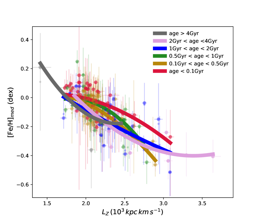
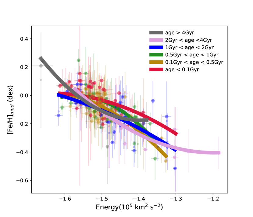
Figure 10: The clusters’ median [Fe/H] as a function of their Z component of the Galactic angular momentum (left panel) and the total Galactic energy (right panel) for all the LAMOST clusters with no less than three flag=12 stars. The solid curves are the second-order polynomial MCMC fittings of each age group.

The nature of the flat metallicity tail is still an open question. Lépine et al. (2011) propose a hypothesis that clusters at the outer Galactic disc with a flat [Fe/H] trend may have their birth place at a smaller $R_{\rm GC}$ . These clusters travel between their orbit pericentre and apocentre, and are observed in their present day position at a larger $R_{\rm GC}$ . This hypothesis could explain the absence of young cluster at the outer Galactic disc and allow a simple trend of metallicity along the Galactic radius. Our metallicity trend with $L_{\rm Z}$ and energy, however, considers both spatial position and motions, thus should not be affected by orbit.

The existence of the flat metallicity tail on the $L_{\rm Z}$ and energy plane, especially the two different flat metallicity tails, must come from an alternative mechanism. Another possible hypothesis proposed by Lépine et al. (2011) is the gas flow from the relative inner region (the corotation radius) of the Galaxy to the external regions, which brings gas with a slightly higher metallicity to the outer regions and flattens the metallicity gradients. The driven of the gas flow could be the gas interaction with the spiral potential perturbation (see detail discussions and simulations in Lépine et al., 2001). With the current set of OC data, we are not able to confirm or exclude this hypothesis. Detailed chemical abundances of the outer disc clusters may help to revive the initial gas composition of these clusters. Whether the gas flow hypothesis can also explain the other flat metallicity tail that of the age $>4$ Gyr clusters requires further investigations.

Another key to understanding the metallicity evolution history of the flat metallicity tail is to investigate the origin of clusters in the Galactic outer disc, namely the clusters with high values of $L_{\rm Z}$ and energy. Such clusters are visible on the right part of both panels in Fig. 10. Are these clusters native residents of our Galaxy, or do they have an extragalactic origin? For instance, the formation and origin of Berkeley 29 – which is the outermost known disc cluster with a $R_{\rm GC}$ of $\sim$20 kpc – are discussed in the literature (Carraro & Bensby, 2009). In their work, Carraro & Bensby (2009) find that the trailing tail of Sgr dSph passes close to the location of Berkeley 29, and their [Mg/Fe], [Ca/Fe] abundances are similar to each other at the same [Fe/H] . They suggest that Berkeley 29 was formed in Sgr dSph and was left on the Galactic disc during one of Sgr dSph’s passages through our Galaxy about 5 Gyr ago. In fact, the mean metallicity of dwarf satellite galaxies may be higher than that of the original outskirts stars of the MW disc. After the satellite galaxy was disrupted by the MW tidal field, the stripped stars distribute mainly on the outer region of MW due to their high kinetic energy and angular momentum. These processes will increase the overall metallicity of the outskirts and form a flat metallicity tail. In a follow-up paper (Chang in prep.), we will discuss in detail the role of minor mergers on forming the flat metallicity tail.

Table 6: The second-order polynomial MCMC fitting parameters of the cluster [Fe/H] as a function of the Galactic radius ($R_{\rm GC}$), the Z component of the Galactic angular momentum ($L_{\rm Z}$), and the total Galactic energy (En) for six age groups, respectively. (a₆, b₆, c₆) stands for the age $>$ 4Gyr group, (a₅, b₅, c₅) stands for the 2Gyr $<$ age $<$ 4Gyr group, (a₄, b₄, c₄) stands for the 1Gyr $<$ age $<$ 2Gyr group, (a₃, b₃, c₃) stands for the 0.5Gyr $<$ age $<$ 1Gyr group, (a₂, b₂, c₂) stands for the 0.1Gyr $<$ age $<$ 0.5Gyr group, and (a₁, b₁, c₁) are the age $<$ 0.1Gyr group. The range of each parameter marks the 16% and 84% of the MCMC fitting sample distribution.

age (Gyr)	par.	RGC	L${}_{Z}/10^{3}$	En$/10^{5}$
	a6	0.066 ${}^{+0.102}_{-0.101}$	0.423 ${}^{+0.706}_{-0.763}$	6.343 ${}^{+9.242}_{-9.366}$
$>4$	b6	-1.379${}^{+2.021}_{-2.038}$	-2.037 ${}^{+3.133}_{-2.890}$	17.821 ${}^{+27.608}_{-27.947}$
	c6	7.019 ${}^{+9.951}_{-9.878}$	2.278 ${}^{+2.965}_{-3.209}$	12.331 ${}^{+20.589}_{-20.830}$
	a5	0.004 ${}^{+0.003}_{-0.003}$	0.177 ${}^{+0.153}_{-0.143}$	3.203 ${}^{+3.122}_{-3.373}$
$[2,4]$	b5	-0.143${}^{+0.090}_{-0.090}$	-1.196 ${}^{+0.809}_{-0.866}$	7.673 ${}^{+8.505}_{-9.148}$
	c5	0.894 ${}^{+0.633}_{-0.629}$	1.621 ${}^{+1.191}_{-1.126}$	4.198 ${}^{+5.765}_{-6.078}$
	a4	0.005 ${}^{+0.008}_{-0.008}$	0.037 ${}^{+0.167}_{-0.229}$	-1.522 ${}^{+3.596}_{-3.235}$
$[1,2]$	b4	-0.170${}^{+0.176}_{-0.176}$	-0.459 ${}^{+1.053}_{-0.765}$	-5.670 ${}^{+10.621}_{-9.556}$
	c4	1.026 ${}^{+0.897}_{-0.898}$	0.685 ${}^{+0.872}_{-1.181}$	-5.182 ${}^{+7.819}_{-7.043}$
	a3	-0.002${}^{+0.009}_{-0.009}$	-0.371 ${}^{+0.187}_{-0.197}$	-6.969 ${}^{+3.223}_{-3.243}$
$[0.5,1]$	b3	-0.017${}^{+0.189}_{-0.190}$	1.349 ${}^{+0.869}_{-0.825}$	-21.900${}^{+9.621}_{-9.671}$
	c3	0.274 ${}^{+0.930}_{-0.925}$	-1.233 ${}^{+0.894}_{-0.940}$	-17.206${}^{+7.164}_{-7.196}$
	a2	-0.009${}^{+0.008}_{-0.008}$	-0.215 ${}^{+0.235}_{-0.173}$	-4.113 ${}^{+2.934}_{-3.074}$
$[0.1,0.5]$	b2	0.122 ${}^{+0.162}_{-0.163}$	0.611 ${}^{+0.811}_{-1.095}$	-13.651${}^{+8.598}_{-9.005}$
	c2	-0.383${}^{+0.833}_{-0.830}$	-0.402 ${}^{+1.238}_{-0.937}$	-11.297${}^{+6.292}_{-6.590}$
	a1	-0.005${}^{+0.012}_{-0.011}$	-0.135 ${}^{+0.252}_{-0.210}$	-2.439 ${}^{+4.097}_{-3.798}$
$<0.1$	b1	0.044 ${}^{+0.205}_{-0.223}$	0.406 ${}^{+0.873}_{-1.053}$	-8.025 ${}^{+12.480}_{-11.586}$
	c1	-0.027${}^{+1.032}_{-0.951}$	-0.277 ${}^{+1.097}_{-0.904}$	-6.577 ${}^{+9.508}_{-8.830}$

One of the most popular and efficient methods to identify different Galactic structures is the Integral Of Motion (IOM) space (see discussions in Helmi, 2020, and references therein). The main idea of this method is using the total energy and the Z component of angular momentum as a long-term record. Stars or clusters with a similar origin tend to cluster in the energy-$L_{\rm Z}$ space.

Fig. 11 shows the IOM of LAMOST OCs. Most clusters lie on a compact region on the IOM space, which represents the dynamical property of the Galactic thin disc. However, a few outliers do exist, in which we highlight a cluster with a small value of both $L_{\rm Z}$ and Energy in the inner part of the Galaxy (NGC 6791), clusters with large values of $L_{\rm Z}$ and Energy in the outer part of the Galaxy (Berkeley 29, Berkeley 34, and Berkeley 19), and clusters showing a departure from the main thin disc property (Berkeley 32, UPK 39, Berkeley 17, and NGC 7128). These clusters must either have a different origin, or have experienced different evolution compared to the majority of normal OCs of the Galactic thin disc.

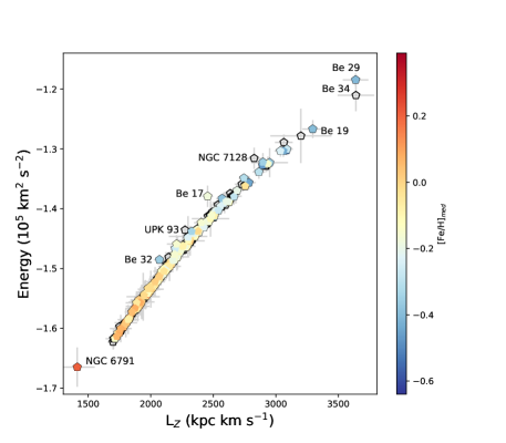
Figure 11: The Integral Of Motion (IOM) of LAMOST OCs with multiple members (N${}_{\sc flag=1}\geq$ 2). The [Fe/H] colour-code is applied to clusters with at least three flag=12 members. The empty symbols are clusters with less than three flag=12 members.

Similar to the Galactic field stars, clusters inhabit and travel on both sides of the Galactic plane. The scale height of the Galactic disc is shaped by the disc stars and OCs. It increases quickly from the Solar $R_{\rm GC}$ to the outer disc on both sides of the plane. This increase in Z distance departure from the Galactic plane is referred as the disc flare. The flare has already been traced with different types of stars, such as blue stragglers (see e.g. Thomas et al., 2019), red clump stars (see e.g. Wan et al., 2017), and red giants (see e.g. Wang et al., 2018).

Using simulations and LAMOST K giant stars, Xu et al. (2020) suggest that the last impact of Sgr dSph contributes to the flare, and identify three different branches of the flare with rotation velocity $V_{\phi}$. According to their results, the boundary of the flare is constructed by stars with a similar $V_{\phi}$ to the main part of the disc stars. The $V_{\phi}$ value for the flare boundary stars is very different compared to halo stars at the same $R_{\rm GC}$ and stars on the disc plane at larger $R_{\rm GC}$ . In Fig. 12 we follow the analysis of Xu et al. (2020) to investigate the LAMOST OCs distribution on the Z-$R_{\rm GC}$ plane. All clusters are colour-coded with their Galactic V_ϕ.

The upper panel shows all LAMOST OCs in our catalogue. It is apparent that the clusters’ Z distances increase toward the outer disc, indicating that OCs can also probe the disc flare. The flare clusters with similar V_ϕ to clusters close to the Galactic plane show an asymmetric structure from the north side to the south side of the Galactic plane. Two sequences of clusters are apparent below the Galactic plane, similar to the south branch and main branch identified by Xu et al. (2020), but less extended. Xu et al. (2020) simulate the disc evolution after the impact of Sgr dSph $\sim$500 Myr ago and conclude that the interaction between the Galactic disc and the dwarf galaxy contribute the flare. To check if OCs are also under the influence of the Sgr dSph passage, we divided our LAMOST OCs into two categories: a young group with age $<500$ Myr, representing clusters born after the last passage of Sgr dSph; and an old group with age $>500$ Myr, representing clusters born before the passage. The two categories are shown in the middle and lower panel of Fig. 12, respectively. We expect clusters in the older category to travel in the Galaxy more like a solid body and behave similarly to field stars, while clusters in the young category should be less affected by the interaction directly because they were gas clouds or even stars of a previous generation, when the impact took place. Indeed, clusters with age ¿ 500 Myr shape the OC flare boundary (see the lower panel of Fig. 12), while clusters with age ¡ 500 Myr are more concentrated along the Galactic plane with a small V_ϕ variation.

We do notice that according to radial migration simulations (see e.g. Minchev et al., 2012), secular evolution of the Galactic disc can increase the scale height in the outer disc and decrease the scale height in the inner region. Thus, it can also produce a flare structure. However, clusters move outward by gaining angular momentum and azimuthal velocity V_ϕ (Schönrich & Binney, 2009) while the low V_ϕ of the LAMOST OCs in the flare region are difficult to reconcile with radial migration. Considering their asymmetric distribution above and under the Galactic plane, we suggest that the disc perturbation introduced by the last impact of Sgr dSph contributes to the OC flare.

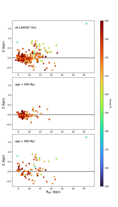
Figure 12: The present-day location of LAMOST OCs on the Z_GC-$R_{\rm GC}$ plane. The upper panel shows all LAMOST OCs, while the middle and lower panels show clusters born after the last passage of the Sgr dSph (age¡500 Myr), and clusters born before the passage (age ¿500 Myr), respectively. Clusters are colour-coded with their azimuthal velocity V_ϕ.

4.2 Connection with nearby molecular clouds

Young clusters are a link between the interstellar medium (ISM) and stellar evolution. Since most stars are born in stellar clusters, linking young clusters to their surrounding molecular clouds offers a great help to understand star formation on a Galactic scale.

Using $Gaia$ DR2 distances and stellar optical and near-infrared photometry, Zucker et al. (2019) present a technique to determine distances of molecular clouds. Zucker et al. (2020) apply this method to $\sim$60 star-forming regions and molecular clouds within 2.5 kpc. To investigate the connections between these clouds and young clusters, we show in Fig.13 the positions of the Zucker et al. (2020) clouds in the Cartesian coordinate X-Y plane (centred on the Sun) and over-plot the young clusters (age $<100$ Myr) of the LAMOST OC sample. Many LAMOST young clusters show an overlap with the molecular clouds on the Galactic plane. With such a young age and a similar Galactic position, they are very likely associated with each other. Since it is easier to obtain metallicity from stars than from molecular clouds, a young cluster is a good probe to study the metallicity evolution of the surrounding molecular clouds. We colour-code clusters in Fig.13 with [Fe/H] in the left panel and cluster age in the right panel. It is clear that even for clusters that share a similar position on the Galactic plane, their [Fe/H] and age differ. This indicates that there are multiple star formation epochs during the past 100 Myr in the Solar neighbourhood, with gas metallicity covering a $\Delta$[Fe/H] $\sim$0.4 dex (i.e. about 2.7 times difference in metallicity). Whether this difference is due to inhomogeneous mixing in the giant molecular cloud, or because of fast star formation and pollution in the past 100 Myr, requires further investigations.

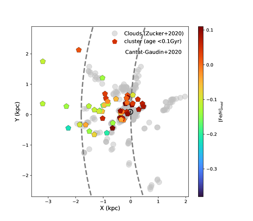
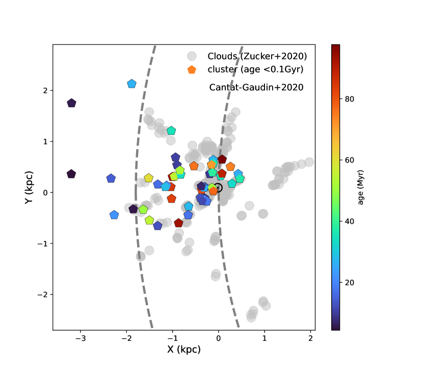
Figure 13: Positions of the age ¡ 0.1 Gyr clusters on the Galactic plane, compared to the nearby molecular clouds from Zucker et al. (2020); Zucker (2019). The two dashed circles indicate a Galactic radius of 8.2 kpc and 10 kpc. The clusters are colour-coded with their median [Fe/H] value in the left panel and with age in the right panel. Only clusters with more than three flag=12 stars are displayed.

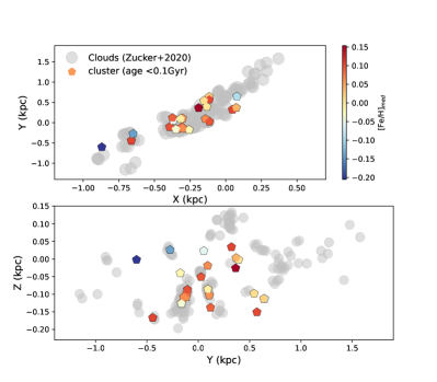
Figure 14: [Fe/H] distribution of clusters along the Radcliffe gas wave. The upper panel is a bird’s eye view and the lower panel is a side view along the Cartesian Y axis. Clusters are colour-coded with their [Fe/H] values.

To study the metallicity distribution along a sequence of nearby molecular clouds, we investigate OCs around the Radcliffe wave, which is a coherent gaseous wave-like structure in the solar neighbourhood reported by Alves et al. (2020) based on the molecular cloud distance catalogue (Zucker et al., 2019, 2020).

Following Alves et al. (2020), we select 24 LAMOST young OCs along the Radcliffe wave. Table 7 lists the Galactic coordinates, Cartesian coordinate XYZ, age, and [Fe/H] of these clusters. They are located along the gas wave clouds in three-dimensional space. Figure 14 shows the spatial distribution of these clusters together with the Radcliffe wave clouds. In both the Cartesian X-Y (upper panel) and Y-Z (lower panel) frame, these clusters show a high spatial consistency with the wave clouds. The metallicities of these clusters, with the higher values in the more central part of the wave, cover a non-negligible range, from sub-solar to super-solar. The highest [Fe/H] is about 1.4 times the Solar metallicity, and the lowest [Fe/H] is about 0.6 times the Solar metallicity. The [Fe/H] distribution of these clusters could be considered as the metallicity distribution of the Radcliffe wave in the past star formation epochs.

Table 7: The Galactic coordinates, age, Cartesian coordinate XYZ (centred on the Sun), age, and [Fe/H] of the 24 very young LAMOST OCs along the Radcliffe wave.

cluster	Glon ($\degree$)	Glat ($\degree$)	age (Myr)	X (pc)	Y (pc)	Z (pc)	[Fe/H]
ASCC_16	201.139	-18.37	13.48	-305	-118	-108	0.06 $\pm$ 0.07
ASCC_21	199.938	-16.60	8.91	-307	-111	-97	0.08 $\pm$ 0.10
ASCC_29	214.743	-0.13	93.32	-869	-602	-2	-0.21 $\pm$ 0.06
Alessi_20	117.615	-3.70	9.33	-190	364	-26	0.15 $\pm$ 0.57
Collinder_69	195.162	-12.05	12.58	-393	-106	-87	0.10 $\pm$ 0.22
Gulliver_6	205.246	-18.14	16.59	-346	-163	-125	0.06 $\pm$ 0.11
IC_348	160.486	-17.81	11.74	-303	107	-103	0.06 $\pm$ 0.13
Melotte_20	147.357	-6.40	51.28	-143	91	-19	0.07 $\pm$ 0.09
Melotte_22	166.462	-23.61	77.62	-114	27	-51	0.10 $\pm$ 0.07
NGC_2183	213.898	-11.84	17.37	-662	-444	-167	0.11 $\pm$ 0.04
NGC_2232	214.458	-7.47	17.78	-257	-176	-40	-0.02 $\pm$ 0.12
NGC_2264	202.941	2.17	27.54	-650	-275	26	-0.14 $\pm$ 0.31
NGC_7063	83.0930	-9.89	97.72	78	646	-113	-0.09 $\pm$ 0.03
RSG_5	81.7190	6.10	34.67	47	323	34	0.11 $\pm$ 0.11
RSG_7	108.781	-0.32	38.90	-133	393	-2	0.00 $\pm$ 0.09
Roslund_6	78.4950	0.58	89.12	74	368	3	0.04 $\pm$ 0.10
Stock_10	171.714	3.56	81.28	-368	53	23	-0.06 $\pm$ 0.10
UPK_166	100.382	-9.91	26.91	-116	638	-113	0.02 $\pm$ 0.26
UPK_168	101.455	-14.58	36.30	-115	571	-151	0.10 $\pm$ 0.10
UPK_185	105.807	-9.94	70.79	-153	543	-98	0.01 $\pm$ 0.04
UBC_17a	205.335	-18.02	18.62	-302	-143	-108	0.06 $\pm$ 0.38
UBC_31	163.527	-14.72	26.30	-317	93	-86	-0.01 $\pm$ 0.08
UBC_17b	205.142	-18.18	11.48	-350	-164	-127	-0.04 $\pm$ 0.09
UBC_19	162.215	-19.48	6.91	-373	119	-138	0.09 $\pm$ 0.10

5 Summary

Using high quality open cluster membership based on $Gaia$ data (Cantat-Gaudin et al., 2020) and spectroscopic results from LAMOST DR8, we obtain a LAMOST OC catalogue with 386 open clusters. The radial velocity and metallicity of these clusters are determined homogeneously. To our knowledge, this is the first radial velocity determination for 44 clusters and the first spectroscopic [Fe/H] determination for 137 clusters. Among the clusters with newly-obtained [Fe/H] , 63 ones are based on at least three member stars with high quality stellar parameter determinations.

The cluster parameter determinations are based on Monte Carlo sampling method. Member stars used for cluster V_rad determinations are marked with flag=1, those used for both V_rad and [Fe/H] determinations are marked with flag=12. The final LAMOST OC parameter catalogue, together with a table of member stars with quality control flag and LAMOST stellar parameters, is available on CDS.

During the quality control process to select flag=12 member stars, we notice a systematic issue of LAMOST cool main sequence stars. Both the surface gravity $\log(g)$ and iron abundance [Fe/H] are under-estimated for main sequence stars with $T_{\mathrm{eff}}$ $\lessapprox$ 5000 K. The problem appears in all clusters that have member stars in this range. These stars are not considered in the cluster parameter determinations. We suggest to take this problem into account also in studies using LAMOST field stars.

Using LAMOST OCs as tracers, we further study the Galactic metallicity distribution and the Galactic disc dynamical properties. We calculate the orbit of the clusters and trace their Galactic metallicity gradient evolution in the past 500 Myr. Since most of the clusters have a non-circular orbit around the Galactic centre, we suggest to use the Z component of the angular momentum L_Z or the total dynamical energy instead of the current Galactic radius $R_{\rm GC}$ to describe the Galactic metallicity gradient. With these two forms of metallicity gradient, we find two flat metallicity trend tails for very old OCs $>$ 4 Gyr and for OCs in the [2 Gyr, 4 Gyr] age range.

We also investigate the OC metallicity distribution in the IOM space. Most of the LAMOST OCs lie in a tight line following the Galactic disc dynamics, while some outlier clusters show different [Fe/H] compared to other clusters in similar IOM space.

LAMOST OCs can be used to trace the Galactic disc flare. The OC flare shows an asymmetric structure above and under the Galactic plane, similar to the field star flare in the literature using LAMOST K giants (Xu et al., 2020). Based on the morphology and V_ϕ distribution of the flare, we suggest that the last impact of Sgr dSph contribute to the OC flare.

The very young LAMOST OCs (age ¡ 100 Myr) are compared to nearby molecular clouds. These young clusters, which are spatially overlapping molecular clouds, can be used to probe star formation history and metallicity evolution of the molecular clouds. We find that even for young clusters with very similar Galactic position, their [Fe/H] and age could differ by a factor of three. This indicates possible inhomogeneous mixing in local ISM (see similar discussions in De Cia et al., 2021) or multiple star formations in OCs during short time scales. Using 24 very young clusters along the Radcliffe wave, we present the metallicity distributions of the gas wave. The nature of this metallicity distribution and its connection to the formation of the Radcliffe wave require further investigations.