Enhancing Space-time Video Super-resolution via Spatial-temporal Feature Interaction

Abstract

The target of space-time video super-resolution (STVSR) is to increase both the frame rate (also referred to as the temporal resolution) and the spatial resolution of a given video. Recent approaches solve STVSR using end-to-end deep neural networks. A popular solution is to first increase the frame rate of the video; then perform feature refinement among different frame features; and at last, increase the spatial resolutions of these features. The temporal correlation among features of different frames is carefully exploited in this process. The spatial correlation among features of different (spatial) resolutions, despite being also very important, is however not emphasized. In this paper, we propose a spatial-temporal feature interaction network to enhance STVSR by exploiting both spatial and temporal correlations among features of different frames and spatial resolutions. Specifically, the spatial-temporal frame interpolation module is introduced to interpolate low- and high-resolution intermediate frame features simultaneously and interactively. The spatial-temporal local and global refinement modules are respectively deployed afterwards to exploit the spatial-temporal correlation among different features for their refinement. Finally, a novel motion consistency loss is employed to enhance the motion continuity among reconstructed frames. We conduct experiments on three standard benchmarks, Vid4, Vimeo-90K and Adobe240, and the results demonstrate that our method improves the state of the art methods by a considerable margin. Our codes will be available at https://github.com/yuezijie/STINet-Space-time-Video-Super-resolution.

1 Introduction

The development of high-definition display techniques, e.g. quantum high dynamic range processor, has enabled the ultra high definition television (UHDTV) which can display videos up to 8K spatial resolution and 240 frames per second (fps) frame rate (also referred to as the temporal resolution of the video). Yet, commonly used video capturing equipment, such as smartphones and web cameras, can only capture full high definition (FHD) videos with a spatial resolution of 2K and a frame rate less than 60 fps [1]. To adapt FHD videos to the UHDTV display for satisfactory visual experience, one promising way is to perform the space-time video super-resolution (STVSR) [2]. STVSR aims to reconstruct videos to their higher spatial and temporal resolution versions. Owing to the clear motion dynamics and fine object details in reconstructed frames, STVSR is beneficial to many applications and has become a research hotspot nowadays.

Traditional STVSR approaches [3, 4, 5] rely on scene-oriented assumptions (e.g. illumination invariance [5]) to align features between given and interpolated frames. This limits their generalizability for complex space-time scenarios [6]. With the advent of deep learning, modern STVSR has been realized as a cascade of video frame interpolation [7, 8, 9] and video super-resolution [10, 11, 12] approaches. Despite their success, these two-stage solutions have drawbacks: the intrinsic relations between spatial and temporal information of video frames are not exploited; the computational cost is also expensive [13, 6].

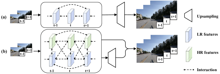
Figure 1: (a) Many advanced STVSR approaches [1, 6, 13, 14, 15] begin with LR features of frames and focus on exploiting their temporal correlation in the network design. (b) Our STINet instead performs a comprehensive spatial-temporal interaction of features with different spatial resolutions (LR and HR) and temporal stamps in STVSR.

To address the above issues, several one-stage STVSR methods have recently been proposed and achieved state of the art performance [16, 15, 1, 6, 13, 14, 17]. Among them, a popular solution (Figure. 1(a)) is to first increase the frame rate of the video, then apply feature refinement among different low-resolution (LR) frame features, and finally increase the spatial resolutions of these features. The whole process is end-to-end optimized. The temporal correlation among different frames, which concerns the information about object deformations and movements along the temporal dimension, is advantageously utilized. On the other hand, the spatial correlation between low- and high-resolution (HR) features, which encodes the complementary spatial information about the texture patterns and structures of objects in images, are not effectively modeled and utilized. We argue that both the spatial and temporal correlations of features are worth exploiting in STVSR so as to capture discriminative spatial-temporal contexts. Our primary motivation is thus to improve STVSR by advantageously performing spatial-temporal feature interaction and refinement (Figure. 1(b)).

We introduce a new end-to-end spatial-temporal feature interaction network (STINet) to enhance STVSR. Given the input of a low-frame-rate low-resolution video, we first initialize its corresponding LR and HR frame features. To interpolate intermediate frame features from them, we design a new spatial-temporal frame interpolation (ST-FI) module consisting of a motion subnet and an interpolation subnet. Shareable blocks are specifically injected into the ST-FI module to facilitate the information interaction between LR and HR features. Having the initialized and interpolated LR and HR features, on one hand, we directly optimize them with their corresponding video ground truth to distinguish between LR and HR predictions for a certain frame; on the other hand, we pass them through several spatial-temporal local refinement (ST-LR) modules, each learns two deformable sampling functions for refining the LR or HR feature with their local neighbors. An interaction subnet is proposed in the ST-LR module to enable the interaction between the predicted sampling offsets in the two functions. Afterwards, we present a spatial-temporal global refinement (ST-GR) module based on a graph convolutional network (GCN). The graph topology and edge attributes are carefully designed to enable the spatial-temporal information passing and exchanging over the whole LR and HR feature sequence. In the end, we fuse the LR and HR features per frame to obtain the high-frame-rate high-resolution video. For the network optimization, we introduce a new motion consistency loss: it computes predicted optical flows across reconstructed frames and defines absolute and relative loss terms to enforce the predictions to conform to either the ground truth or the motion continuity between frames.

In summary, the main contribution of this paper is below:

1. We introduce a novel end-to-end architecture to explicitly perform spatial-temporal feature interaction in STVSR.

2. Three key modules are highlighted: the spatial-temporal frame interpolation module, the spatial-temporal local refinement module, and the spatial-temporal global refinement module. They are carefully designed for comprehensive spatial-temporal feature interaction.

3. A new motion consistency loss is designed to integrate the motion factor into the network optimization.

4. Our method significantly outperforms the state of the art approaches on standard benchmarks Vid4 [18], Vimeo-90K [19] and Adobe240 [20].

Besides above, we notice that most state of the art STVSR solutions can only support single frame interpolation between two adjacent frames whereas in reality we would need multi-frame interpolation to display a FHD video on an UHDTV. To achieve this, we enable our STINet with controllable frame interpolation rate.

2 Related work

2.1 Video frame interpolation

Video frame interpolation (VFI) synthesizes intermediate frames between temporally neighboring frames in the same level of spatial resolution. It can be mainly implemented as kernel-based [21, 22, 7] or flow-based [23, 24, 25, 26] approaches. Kernel-based approaches generate intermediate frames by designing special convolutional kernels in deep neural networks to convolve on adjacent frames. For instance, Lee et al. [21] proposed the spatially-adaptive convolution kernel to map pixels in given frames to proper locations in the intermediate frame. Shi et al. [22] introduced the generalized deformable convolution kernels to select existing pixels for synthesizing new pixels. Flow-based approaches predict flows to map pixels from adjacent frames to new locations in the intermediate frame. For instance, Niklaus et al.  [24] estimated bidirectional optical flows between given frames and passed them with corresponding pixel-level context maps to a frame synthesis network. To reduce artifacts around boundaries of moving objects in intermediate frames, Jiang et al.  [23] employed two consecutive U-Nets to refine the estimated optical flows before feeding them into the frame synthesis network. Huang et al.  [26] designed a knowledge distillation model which constrains flows predicted from the student model to be consistent with that from the teacher model.

2.2 Video super-resolution

Video super-resolution (VSR) is to reconstruct HR frames from their LR counterparts. Existing approaches perform VSR in two main steps [19, 27, 28, 29]: first, aggregating spatial information from the reference and its neighboring LR frames; second, performing feature alignment and warping to reconstruct the corresponding HR frame. Haris et al.  [29] iteratively calculated the residual maps to capture spatial context differences between the reference and neighboring LR frames, then back-projected these residuals on the reference frame to produce its HR version. Jo et al. [30] predicted dynamics upsampling filters via a dynamic filter generation network, which are then used to filter LR frames for enlarging their spatial resolutions. Zhang et al. [31] designed a multi-branch network to learn multi-scale spatial features from LR frames to boost the VSR performance. Other methods have utilized the convolutional LSTM [32], generative adversarial network [33], and graph neural network [34] to reconstruct HR frames.

2.3 Space-time video super-resolution

Space-time video super-resolution (STVSR) aims to increase both the spatial and temporal resolutions of videos. Many traditional approaches rely on scene-oriented assumptions to assist the feature alignment between adjacent LR frames before reconstructing HR frames [3, 4, 5]. For example, Mudenagudi et al.  [5] assumed no illumination changes among neighboring frames and employed the graph-cut optimization to reconstruct high-frame-rate HR videos from low-frame-rate LR videos. Recently, deep learning models have demonstrated robust feature alignment and refinement capabilities in STVSR [16, 1, 6, 13, 14, 35, 15, 36, 37, 17]. Xiang et al.  [6] designed the deformable feature alignment functions to perform intermediate frame interpolation. Xu et al.  [13] enabled the frame reconstruction at an arbitrary intermediate moment. Shi et al.  [17] developed the generalized Pixelshuffle layer to make the spatial resolution of reconstructed videos controllable. Geng et al.  [14] designed a cascaded U-Net style structure to achieve comparable performance with state of the art in STVSR yet using lesser network parameters. Cao et al.  [15] proposed a Fourier data transform layer and a recurrent video enhancement layer to respectively solve the motion blur and motion aliasing problems in the reconstructed videos.

2.4 Comparison of ours to state of the art

The designing spirit of our STINet is to enhance the spatial-temporal feature interaction, which has not been explicitly exploited before in the STVSR task. As mentioned in Sec. 1, many state of the art approaches [1, 17, 6, 13, 14, 15, 35] begin with LR features of frames and focus on exploiting their temporal correlation. [16] has tried to apply local refinement from HR features to LR features or vice versa but there is no mutual information exchange in this process. In contrast, we propose three key modules (ST-FI, ST-LR, and ST-GR) and one motion consistency loss (MCL) to allow HR and LR features comprehensively interacted throughout the network both locally and globally. Particularly, for the local feature refinement, we follow [6, 13, 38] to utilize the deformable convolutional network (DCN) [39] to learn offsets for feature alignment, but our ST-LR module learns two sets of offsets with low and high spatial resolutions respectively and includes a new interaction subnet to enable their interaction. For the global feature refinement, unlike the bidirectional deformable ConvLSTM (BDConvLSTM) used in [6, 13], our ST-GR module builds upon the GCN with a special design of the graph over the whole sequence of LR and HR features to exploit their spatial-temporal correlation. Last, different from the frame reconstruction loss used in [16, 17, 6, 13, 35, 14, 15], we introduce a new MCL to reinforce the motion continuity between frames in the reconstructed video.

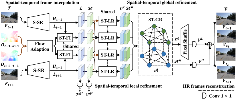
Figure 2: STINet contains four main phases. Phase 1: we initialize the LR and HR features of given frames and interpolate intermediate frame features in the proposed ST-FI module. Phase 2: we pass the LR and HR features into a number of shareable ST-LR modules to capture motion cues from neighboring frames for local feature refinement. Phase 3: we construct a graph network in the ST-GR module which passes complementary spatial-temporal information over whole feature sequence for global feature refinement. Phase 4: we fuse LR and HR features to reconstruct high-frame-rate HR video sequence $\mathcal{V}$.

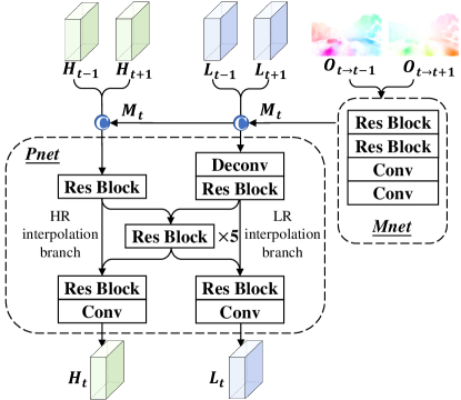
Figure 3: The ST-FI module interpolates intermediate features ($L_{t}$, $H_{t}$) based on both optical flows (${O}_{t\rightarrow{t-1}}$, ${O}_{t\rightarrow{t+1}}$) and initialized LR and HR features ($L_{t-1}$, $L_{t+1}$, $H_{t-1}$, $H_{t+1}$).

3 Method

3.1 Overview

The overview of our STINet is illustrated in Figure. 2. Our goal is to reconstruct the corresponding high-frame-rate HR video sequence $\mathcal{V}$ from the input of low-frame-rate LR video sequence $\mathcal{F}$. STINet contains four phases: spatial-temporal feature interpolation (ST-FI), spatial-temporal local and global refinements (ST-LR and ST-GR), and finally HR frames reconstruction. ST-FI produces LR and HR features of frames, which enables both the spatial (e.g. texture patterns and structures of objects) and temporal (e.g. deformations and movements of objects) information interaction among features of different resolutions and frames. ST-LR and ST-GR elicit the spatial-temporal correlation of features for their local and global refinement, respectively.

Specifically, given two adjacent LR frames $F_{t-1}$ and $F_{t+1}$, we can calculate their bidirectional optical flows ${O}_{t-1\rightarrow{t+1}}$ and ${O}_{t+1\rightarrow{t-1}}$. We first initialize the LR and HR features, i.e. $L_{t-1}$ and $H_{t-1}$, $L_{t+1}$ and $H_{t+1}$, for $F_{t-1}$ and $F_{t+1}$, respectively. The initialization is through the spatial super-resolution (S-SR) module [40], which for instance takes the input of $F_{t-1}$ to output $H_{t-1}$ and $L_{t-1}$. To synthesize intermediate frame features, we adapt ${O}_{t-1\rightarrow{t+1}}$ and ${O}_{t+1\rightarrow{t-1}}$ to obtain optical flows from the target intermediate frame to adjacent frames. Using adapted optical flows as input together with $L_{t-1}$ and $L_{t+1}$ or $H_{t-1}$ and $H_{t+1}$, we interpolate intermediate LR and HR frame features through a spatial-temporal frame interpolation (ST-FI) module (Sec. 3.2). Having LR and HR feature sequences, i.e. $\mathcal{L}=\{L_{t}\}$, $\mathcal{H}=\{H_{t}\}$, on one hand, we optimize them with the corresponding video ground truth i.e. $\mathcal{F}^{gt}$ and $\mathcal{V}^{gt}$, to enforce them to learn the discriminative information; on the other hand, we pass them through several shareable spatial-temporal local refinement (ST-LR) modules to refine each frame feature by its neighbors (Sec. 3.3). Afterwards, we feed the locally-refined features ${\mathcal{L}^{R}}$ and ${\mathcal{H}^{R}}$ to a spatial-temporal global refinement (ST-GR) module to further refine them over the whole sequence (Sec. 3.4), output denoted by ${\mathcal{L}^{G}}$ and ${\mathcal{H}^{G}}$. In the end, we project ${\mathcal{L}^{G}}$ via two Pixelshuffle layers [41] followed by a $1\times 1$ convolutional layer and project ${\mathcal{H}^{G}}$ directly by a $1\times 1$ convolutional layer to obtain the corresponding video frames ${\mathcal{V}^{L}}$ and ${\mathcal{V}^{H}}$, respectively. ${\mathcal{V}^{L}}$ and ${\mathcal{V}^{H}}$ are added to produce the final HR frames $\mathcal{V}$ (Sec. 3.5).

Our network supports multi-frame interpolation given two adjacent frames ($F_{t-1}$ and $F_{t+1}$), as illustrated by Figure. 2. Without loss of generality, below we present it for interpolating a single frame ($t$-th frame $V_{t}$).

3.2 Spatial-temporal feature interpolation

At this phase, we first introduce an optical flow adaption method to obtain optical flows from each intermediate frame to adjacent frames; next, since LR and HR features encode the complementary spatial information about the texture patterns and structures of objects, we design the ST-FI module with a novel interpolation subnet to perform LR and HR feature interaction during the intermediate feature interpolation.

First, in order to interpolate intermediate frame features from features of adjacent frames, we follow flow-based methods [17, 23, 24] to rely on optical flows which describe the velocity distribution of object movement between frames. Different from them, we propose a simple yet effective way to obtain optical flows between the target intermediate frame and their adjacent frames. Having the flows between $F_{t-1}$ and $F_{t+1}$, i.e. ${O}_{t-1\rightarrow{t+1}}$ and ${O}_{t+1\rightarrow{t-1}}$, to adapt them to represent motion information from the frame of an arbitrary moment $t^{\prime}\in(t-1,t+1)$ to that of moment $t-1$/$t+1$, we assume the motion change within the short period ($t+1-(t-1)=2$) is linear, such that:

$$\begin{split}{O}_{t^{\prime}\rightarrow{t-1}}=\frac{t^{\prime}-(t-1)}{2}\times O_{t+1\rightarrow t-1}\\ {O}_{t^{\prime}\rightarrow{t+1}}=\frac{(t+1)-t^{\prime}}{2}\times{O}_{{t-1}\rightarrow{t+1}}\end{split}$$ (1)

This equation can be used for the multi-frame interpolation. For simplicity, here we use $t^{\prime}=t$, so ${O}_{t\rightarrow{t-1}}=0.5\times{O}_{{t+1}\rightarrow{t-1}}$, ${O}_{t\rightarrow{t+1}}=0.5\times{O}_{{t-1}\rightarrow{t+1}}$.

Next, we perform LR and HR intermediate feature interpolation via a spatial-temporal feature interpolation (ST-FI) module. Its structure is shown in Figure. 3, which consists of a motion subnet (Mnet) and an interpolation subnet (Pnet).  The Mnet is inspired by [16] to model a motion representation $M_{t}$ from ${O}_{t\rightarrow{t-1}}$ and ${O}_{t\rightarrow{t+1}}$, which can help spatial alignment from given features to intermediate ones. It is composed of two residual blocks and two convolutional layers.

The Pnet is designed to take the input of $M_{t}$, $L_{t-1}$, $L_{t+1}$, $H_{t-1}$ and $H_{t+1}$ to synthesize intermediate frame features $L_{t}$ and $H_{t}$: We concatenate $M_{t}$ with $L_{t-1}$ ($H_{t-1}$) and $L_{t+1}$ ($H_{t-1}$) as an input for the LR (HR) interpolation branch, respectively. The two branches are jointed through five shareable residual blocks, which help encode mutual and complementary contexts among frame features of different spatial-temporal information. Skip connection is applied to concatenate the input and output of these shareable blocks for LR or HR interpolation branch.

The output feature sequences, $\mathcal{L}=\{L_{t}\}$ and $\mathcal{H}=\{H_{t}\}$ for LR and HR features of both intermediate and adjacent frames, are passed through separated $1\times 1$ convs and supervised by the corresponding ground truth, $\mathcal{F}^{gt}$ and $\mathcal{V}^{gt}$.

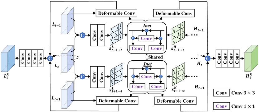
Figure 4: An example architecture of the ST-LR module which takes the input of $L_{t-1}$, $L_{t}$, and $L_{t+1}$ from the left side, and $H_{t-1}$, $H_{t}$, and $H_{t+1}$ from the right side to refine $L_{t}$ and $H_{t}$.

3.3 Spatial-temporal local refinement

This phase aims to refine LR and HR features of each frame by extracting short-term motion cues from their temporal neighbors and learning deformable sampling functions [6, 13]. Specifically, we learn one set of sampling offsets for each LR or HR feature with its certain neighbor, respectively, and enable the information exchange between the learned two sets of offsets via a new interaction subnet.

Figure. 4 illustrates an example of ST-LR that refines $L_{t}$($H_{t}$) using $L_{t-1}$($H_{t-1}$) and $L_{t+1}$($H_{t+1}$). Having a look at the left side, we concatenate $L_{t}$ with $L_{t-1}$ and $L_{t+1}$ respectively and utilize two convolutional layers each to predict the offsets ${s}_{{t-1}\rightarrow t}^{L}$ and ${s}_{{t+1}\rightarrow t}^{L}$. These offsets implicitly describe the forward and backward motion cues from $L_{t-1}$ and $L_{t+1}$ to $L_{t}$. Similar offsets ${s}_{{t-1}\rightarrow{t}}^{H}$ and ${s}_{{t+1}\rightarrow{t}}^{H}$ can be estimated from HR features $\left\{H_{t-1},H_{t},H_{t+1}\right\}$ in the right side. The corresponding offsets pairs, ${s}_{{t-1}\rightarrow{t}}^{L}$ and ${s}_{{t-1}\rightarrow{t}}^{H}$, ${s}_{{t+1}\rightarrow{t}}^{L}$ and ${s}_{{t+1}\rightarrow{t}}^{H}$, are of different resolutions and are fed into a shareable interaction subnet (Inet, specified below) for information exchange. The refined offsets are served as the kernel parameters for deformable convolutional networks (DCN) [39], which are used to align $L_{t-1}$/$L_{t+1}$ towards $L_{t}$, and $H_{t-1}$/$H_{t+1}$ towards $H_{t}$. Last, we respectively concatenate $L_{t}$ and $H_{t}$ with the aligned feature maps and apply four convolutional layers each to obtain locally-refined features ${L_{t}^{R}}$ and ${H_{t}^{R}}$.

We specify our Inet by taking an example of ${s}_{{t-1}\rightarrow{t}}^{L}$ and ${s}_{{t-1}\rightarrow{t}}^{H}$. They are first concatenated and passed through a convolutional layer to capture their complementary information regarding the short-term object motions between $t-1$ and $t$-th frames. The output is respectively concatenated with the original input ${s}_{{t-1}\rightarrow{t}}^{L}$ and ${s}_{{t-1}\rightarrow{t}}^{H}$ followed by one convolutional layer each to produce the refined offsets, $\widehat{s}_{{t-1}\rightarrow{t}}^{L}$ and $\widehat{s}_{{t-1}\rightarrow{t}}^{H}$. This can be understood as a modulation process on the input ${s}_{{t-1}\rightarrow{t}}^{L}$ and ${s}_{{t-1}\rightarrow{t}}^{H}$, which enhances their salient information while suppressing their trivial information. Backward offsets ${\widehat{s}}_{{t+1}\rightarrow{t}}^{L}$ and ${\widehat{s}}_{{t+1}\rightarrow{t}}^{H}$ can be obtained similarly.

The ST-LR module is applied to each feature in $\mathcal{L}$ and $\mathcal{H}$ with a sliding window of size 3. For the first (last) feature in the sequence, its previous (next) neighbor is itself. By the end of this phase, we have refined features ${\mathcal{L}^{R}}$ and ${\mathcal{H}^{R}}$.

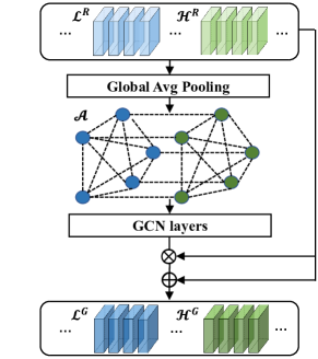
Figure 5: The ST-GR module performs globally spatial-temporal information passing and exchanging over the whole feature sequence via the graph convolutional network (GCN).

3.4 Spatial-temporal global refinement

This phase aims to refine features of each frame over the whole sequence. Since the graph convolutional network (GCN) has been proved effective in video matting [42] and object tracking [43] tasks for its powerful information aggregation ability, we build the ST-GR module upon the GCN. We introduce a novel way to define the edges and edge attributes among different frame features based on their spatial-temporal correlation. It can thus globally exchange the complementary information regarding object spatial structures and temporal movements among LR and HR features of different frames. The graph topology is particularly suitable for this purpose. This can not be achieved by the BDConvLSTMas used in [6, 13]. BDConvLSTM is good at encoding temporal correlation among frames but not spatial correlation among features with different resolutions. Below, we specify our module, its structure is illustrated in Figure. 5.

Features in ${\mathcal{L}^{R}}$ and ${\mathcal{H}^{R}}$ are of dimension $w\times h\times c$. They are firstly fed into a global-average pooling layer to obtain the frame-level global features of dimension $1\times 1\times c$, which are used as node features to construct the graph $\mathcal{A}$. The structure of $\mathcal{A}$ is defined by an adjacency matrix, which represents the connections among nodes. First, each node is connected to its corresponding HR or LR counterpart as they describe the same frame of different spatial resolutions. Second, each node is connected to other nodes of the same spatial-resolution level yet different frames. The connections enable both spatial and temporal correlations between features.

Next, for each connection (edge), we define the edge attribute as a triplet $E=(E^{F},E^{P},E^{T})$ of three factors: 1) Frame-level similarity $E^{F}$ measures the cosine similarity between the frame-level global features (node features) of two connected nodes; 2) Pixel-level similarity $E^{P}$ averages the cosine similarities between pixel-level features (pixel-wise features taken from the $w\times h\times c$ tensor of $L^{R}$/$H^{R}$) of two connected nodes. For the calculation between features with different spatial resolutions, we downsample HR features to match the resolution of LR ones; 3) Temporal closeness $E^{T}$ measures the temporal-distance of two connected nodes. Given the time stamps of $t_{1}$ and $t_{2}$ for two nodes, $E^{T}$ is computed as $1-\sigma\left(\left|t_{1}-t_{2}\right|\right)$; $\sigma$ indicates the sigmoid function. $E^{F}$ and $E^{P}$ measure the globally/locally visual similarity of two features. $E^{T}$ measures the temporal closeness of two frames. For any two nodes that are either visually similar or temporally close, they are assigned with bigger weights by $E^{F},E^{P}$ or $E^{T}$ such that more spatial-temporal information will be exchanged through them in the graph.

Once $\mathcal{A}$ is initialized, we feed the node features together with their connections defined in $\mathcal{A}$ into four GraphSAGE layers [44] to perform spatial-temporal information passing and exchanging for global refinement. Each output node feature ($1\times 1\times c$) is channel-wisely multiplied to its corresponding original HR/LR feature ($w\times h\times c$); the resulting feature serves as a modulation term and is added back to the original feature for refinement. We denote the output of this module by ${\mathcal{L}^{G}}=\left\{L_{t}^{G}\right\}$ and ${\mathcal{H}^{G}}=\left\{H_{t}^{G}\right\}$ for LR and HR feature sequences.

3.5 High-frame-rate High Resolution Video Reconstruction

We follow [13] to feed ${\mathcal{L}^{G}}$ into two Pixelshuffle layers for spatial super-resolution. They are followed by a $1\times 1$ convolutional layer to project the features to 2-dimensional images $\mathcal{V}^{L}$. ${\mathcal{H}^{G}}$ is projected via another $1\times 1$ convolutional layer to obtain $\mathcal{V}^{H}$. They are added to obtain the high-frame-rate HR video $\mathcal{V}=\left\{V_{t}\right\}$: ${V_{t}={V_{t}^{L}}+{V}_{t}^{H}}$.

3.6 Network optimization

Three loss functions are leveraged to optimize the network parameters: the reconstruction loss, the perceptual loss, and the motion consistency loss. The former two are commonly used in STVSR approaches [16, 17, 6, 13, 14]: $l_{rec}=\sum_{t=1}^{N}{\left\|V_{t}-V_{t}^{gt}\right\|}_{2}^{2}$; $l_{per}=\sum_{t=1}^{N}{\left\|\phi(V_{t})-\phi(V_{t}^{gt})\right\|}_{2}^{2}$, where $V_{t}$ and $V_{t}^{gt}$ signifies the prediction and ground truth of $t$-th HR frame; $N$ is the total number of frames; $\phi(\cdot)$ is the feature extractor of the pretrained VGG-19 [45].

Motion consistency loss (MCL). $l_{rec}$ and $l_{per}$ measures the pixel-level and frame-level visual differences between the prediction and ground truth. We propose a novel motion consistency loss to integrate the temporal factor into the optimization, which can help reconstruct motions between frames more accurately. To elicit such temporal information from our predictions, we compute the optical flows between any two predicted frames, i.e. ${O}_{t\rightarrow{p}}^{pred}$ for HR frames $V_{t}$ and $V_{p}$. MCL is defined on the estimated optical flows consisting of two sub terms: the absolute and relative loss. For the absolute loss, we obtain the ground truth optical flows $\mathcal{O}^{gt}$ from $\mathcal{V}^{gt}$, e.g. ${O}_{t\rightarrow{p}}^{gt}$ for HR ground truth frames $V_{t}^{gt}$ and $V_{p}^{gt}$, and compute the mean squared error between the estimated and ground truth flow maps:

$$l_{abs}=\sum_{t=1}^{N}\sum_{p=1}^{N}\left\|{O}_{t\rightarrow{p}}^{pred}-{O}_{t\rightarrow{p}}^{gt}\right\|_{2}^{2}.$$ (2)

Notice [26, 37] have a similar flow loss to Eqn.2 but they only supervise flows between adjacent frames which can be seen as a special case of Eqn.2. Moreoever, they use L1 loss while we use L2 loss as L2 loss works better for us empirically.

For the relative loss, our observation is that objects move smoothly over frames and their motions are normally accumulated towards a certain direction over a short period of time. This means, given three consecutive HR frames, $V_{t-1}$, $V_{t}$ and $V_{t+1}$, the motions of objects between frame $V_{t-1}$ and $V_{t+1}$ should normally be bigger than that between $V_{t-1}$ and $V_{t}$. In practice, we use optical flows to represent motions and define a novel loss $l_{rel}$,

$$\begin{split}l_{rel}=\sum_{t=2}^{N-1}{\sum_{i=1}^{I}\sum_{j=1}^{2}max(sgn({O}_{t-1\rightarrow t,i,j}^{pred})\times}{({O}_{t-1\rightarrow t,i,j}^{pred}-{O}_{t-1\rightarrow t+1,i,j}^{pred}),0)}\end{split}$$ (3)

where $i,j$ represent the $i$-th pixel $j$-th channel of the optical flows. There are in total $I$ pixels and 2 channels ($x$ and $y$ coordinates). $sgn$ indicates the sign (motion direction) of ${O}_{t-1\rightarrow t,i,j}^{pred}$. The interior loss equals to zero as long as ${O}_{t-1\rightarrow t,i,j}^{pred}$ has the same motion direction with ${O}_{t-1\rightarrow{t+1},i,j}^{pred}$ and $|{O}_{t-1\rightarrow t,i,j}^{pred}|$ is smaller than $|{O}_{t-1\rightarrow{t+1},i,j}^{pred}|$, which agrees with the above motion constraint. We apply a rather weak constraint here to avoid over-fitting, especially since we already have a strong constraint in the absolute term. In practice, the relative term brings more benefits to the STVSR performance than the absolute term in MCL.

The overall loss function is a linear combination of the above losses:

$$l=l_{rec}+l^{\prime}_{rec}+\lambda_{1}\times l_{per}+\lambda_{2}\times l_{mcl},$$ (4)

where $l_{mcl}=l_{abs}+l_{rel}$. We use $l^{\prime}_{rec}$ to represent the reconstruction loss we add at Phase 1 (Sec. 3.2). Adding $l_{per}$ and $l_{mcl}$ at Phase 1 does not offer additional improvement in practice. $\lambda_{1}$ and $\lambda_{2}$ are loss weights.

4 Experiments

4.1 Datasets

The training set of this work is Vimeo-90K septuplet dataset [19], which is widely used in previous STVSR approaches [6, 13, 14]. This dataset contains 91,701 video sequences of resolution $448\times 256$. Each sequence contains 7 HR frames. Following [6], we downsample the odd-index frames of each video sequence to their LR counterparts of resolution $112\times 64$ using bicubic interpolation. They are used as the training inputs to reconstruct original 7 HR frames. To evaluate our method, we follow [6, 13, 14] to use the Vid4 [18], Vimeo-90K septuplet test set and Adobe240 [20]. The Vimeo-90K septuplet test set is split into three subsets corresponding to fast, medium and slow motions; there are 1225, 4977 and 1613 video sequences in each subset, respectively.

4.2 Implementation details and evaluation protocol

Implementation details. We initialize the learning rate as $1\times{10}^{-4}$ and decrease it by a factor of 4 for every ${10}^{5}$ iterations. The total number of iterations is $5\times{10}^{5}$ with the batch size being 30. Network parameters are initialized using Kaiming initialization [46] and optimized by the Adam optimizer [47] with a momentum of 0.9. Moreover, following [6], the input LR frames are randomly cropped to $32\times 32$ image patches, while their corresponding $128\times 128$ image patches in HR frames are treated as ground truth. The training set is augmented by randomly flipping, rotating (${180}^{\circ}$) and mirroring. Loss weights $\lambda_{1}$ and $\lambda_{2}$ are both $0.1$. All experiments were performed on four NVIDIA RTX 2080 GPUs.

Evaluation protocol. Like in [6, 13, 14], the Peak Signal-to-Noise Ratio (PSNR) and Structural Similarity Index (SSIM) [48] metrics are leveraged to evaluate the performance. PSNR measures pixel-level reconstruction errors between the prediction and ground truth, while SSIM compares the luminance, contrast and structure differences in the frame-level. By default, we perform single frame interpolation as per most comparable methods [16, 17, 6, 13, 14]. Results of multi-frame interpolation are also provided.

Table 1: Comparison of STINet to state of the art two-stage (top block) and one-stage (middle block) STVSR approaches. The speed is calculated on Vid4 [18]. $\uparrow$ indicates that the larger the better. We indicate the best performing two-stage approaches in shadow. We highlight the best and second best performing one-stage approaches in red and blue.

Method	Vid4		Vimeo-Fast		Vimeo-Medium		Vimeo-Slow		Adobe240		Speed
VFI+VSR/STVSR	PSNR$\uparrow$	SSIM$\uparrow$	PSNR$\uparrow$	SSIM$\uparrow$	PSNR$\uparrow$	SSIM$\uparrow$	PSNR$\uparrow$	SSIM$\uparrow$	PSNR$\uparrow$	SSIM$\uparrow$	fps$\uparrow$
SepConv[49]+Bicubic	23.51	0.6273	32.27	0.8890	30.61	0.8633	29.04	0.8290	26.61	0.7457	-
SepConv[49]+RCAN[50]	24.92	0.7236	34.97	0.9195	33.59	0.9125	32.13	0.8967	26.84	0.7488	2.42
SepConv[49]+RBPN[29]	26.08	0.7751	35.07	0.9238	34.09	0.9229	32.77	0.9090	30.18	0.8706	2.01
SepConv[49]+EDVR[51]	25.93	0.7792	35.23	0.9252	34.22	0.9240	32.96	0.9112	30.28	0.8745	6.36
DAIN[7]+Bicubic	23.55	0.6268	32.41	0.8910	30.67	0.8636	29.06	0.8289	26.61	0.7453	-
DAIN[7]+RCAN[50]	25.03	0.7261	35.27	0.9242	33.82	0.9146	32.26	0.8974	26.86	0.7489	2.23
DAIN[7]+RBPN[29]	25.96	0.7784	35.55	0.9300	34.45	0.9262	32.92	0.9097	30.29	0.8709	1.88
DAIN[7]+EDVR[51]	26.12	0.7836	35.81	0.9323	34.66	0.9281	33.11	0.9119	30.40	0.8749	5.20
BMBC[52]+TTVSR[53]	26.14	0.7920	35.98	0.9330	34.67	0.9287	33.14	0.9123	30.32	0.8698	1.20
BMBC[52]+ETDM[54]	26.20	0.7926	36.00	0.9347	34.75	0.9288	33.14	0.9126	30.40	0.8711	1.19
ABME[55] +TTVSR[53]	26.30	0.7937	36.23	0.9358	35.00	0.9352	33.20	0.9134	30.59	0.8754	3.56
ABME[55]+ETDM[54]	26.38	0.7958	36.24	0.9365	35.08	0.9355	33.28	0.9138	30.54	0.8750	3.45
STARnet [16]	26.06	0.8046	36.19	0.9368	34.86	0.9356	33.10	0.9164	29.92	0.8589	14.08
Zooming Slow-Mo [6]	26.31	0.7976	36.81	0.9415	35.41	0.9361	33.36	0.9138	30.34	0.8713	16.50
DAVSR [15]	23.85	0.7460	-	-	-	-	-	-	-	-	-
TMNet [13]	26.43	0.8016	37.04	0.9435	35.60	0.9380	33.51	0.9159	30.59	0.8760	14.69
VideoINR [35]	25.61	0.7709	-	-	-	-	-	-	29.92	0.8746	-
RSTT-L [14]	26.43	0.7994	36.80	0.9403	35.66	0.9381	33.50	0.9147	-	-	14.98
STINet(Ours)	26.79	0.8049	37.43	0.9465	35.87	0.9390	34.04	0.9180	30.75	0.8769	14.80
STINet w/o HR	26.34	0.8025	36.96	0.9385	35.39	0.9361	33.55	0.9160	30.44	0.8720	17.17
STINet w/o LR	26.43	0.8027	37.10	0.9440	35.41	0.9337	33.68	0.9164	30.58	0.8736	15.54
STINet w/o ST-LR	25.41	0.7477	35.97	0.9344	34.28	0.9240	32.70	0.9016	29.10	0.8248	16.21
STINet w/o ST-GR	25.94	0.7785	36.70	0.9400	35.11	0.9348	33.24	0.9130	29.69	0.8365	16.46
STINet w/o MCL	26.53	0.8037	37.11	0.9443	35.70	0.9362	33.82	0.9165	30.60	0.8743	14.80

4.3 Comparison to state of the art

The state of the art can be divided into two-stage and one-stage approaches. For two-stage approaches, we leverage the combination of latest VFI (SepConv [49], DAIN [7], BMBC[52], ABME[55]) and VSR (Bicubic, RCAN [50], RBPN [29], EDVR [51], ETDM[54], TTVSR[53]) models to achieve STVSR. For one-stage approaches, Zooming Slow-Mo [6], STARnet [16], DAVSR [15], TMNet [13], VideoINR [35] and RSTT-L [14] are compared.

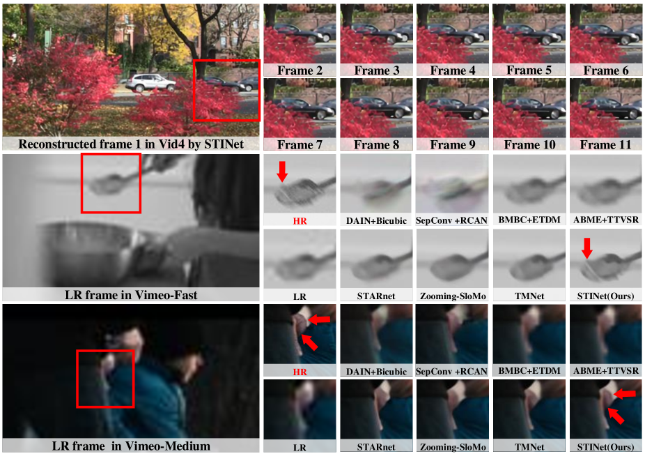
Figure 6: Visual comparison between different STVSR approaches. Our STINet show more visually appealing results than others (zoom in for more details). Ground truth is given as HR.

Table 1 shows the results. For two-stage approaches, having a combination of more recent VFI and VSR models can produce better results than older ones: e.g. ABME + ETDM performs the best. Two-stage approaches treat spatial and temporal information separately while ignoring their correlation, their performance is in general inferior to one-stage approaches. Our STINet significantly outperforms the best performing two-stage approach ABME+ETDM by 0.41dB, 1.19dB, 0.79dB, 0.76dB, 0.21dB on PSNR over five test sets. With respect to the comparison to one-stage approaches, STINet also clearly outperforms all of them on both PSNR and SSIM metrics. For example, on the Vid4 dataset, STINet improves the very recent work [14] by +0.36dB on PSNR and +0.0055 on SSIM.

Besides the reconstruction result, Table 1 also shows that the inference speed of interpolating a single HR frame by STINet is 14.80fps, which is also on par with state of the art. Moreover, the number of parameters for STINet is 11.76M, which is also comparable to that of state of the art, i.e. Zooming Slow-Mo [6] (11.10M), TMNet [13] (12.26M) and VideoINR [35] (11.31M). We’d like to mention that our ST-GR module has saved a lot of parameters compared to the BDConvLSTM layers utilized in [6, 13].

Qualitative results are presented in Figure. 6: in the first row, we show 11 consecutive frames reconstructed by our STINet. We can observe the reconstructed cars with clear textures and smooth movements across frames. In the middle and last rows, we show one-stage approaches produce images with higher qualities and finer details than two-stage ones. For instance, in the middle row, two-stage approaches produce blurring artifacts on the shovel because of its fast motion, while one-stage approaches can reconstruct sharper edges. Furthermore, STINet shows more visually appealing results than others compared to the ground truth, especially on the edges and textures of objects. For instance, in the third row, its reconstructed edges are clearer than others and the color difference between finger and wrist is more obvious.

Table 2: Results on multi-frame interpolation. Method(3) and Method(5) indicate interpolating 3 and 5 frames given two adjacent frames.

	Vid4		Vimeo-Fast		Vimeo-Medium		Vimeo-Slow		Adobe240
Method	PSNR	SSIM	PSNR	SSIM	PSNR	SSIM	PSNR	SSIM	PSNR	SSIM
TMNet(3)	25.45	0.7488	36.28	0.9320	34.52	0.9273	32.75	0.9059	29.44	0.8315
STINet(3)	25.55	0.7579	36.41	0.9335	34.66	0.9280	32.91	0.9086	29.57	0.8323
TMNet(5)	23.72	0.6445	34.74	0.9258	32.70	0.9054	31.26	0.8720	28.03	0.8162
STINet(5)	23.88	0.6557	34.82	0.9277	32.97	0.9095	31.40	0.8786	28.30	0.8176

Table 3: Ablation study on the adapted optical flows.

	Vid4		Vimeo-Fast		Vimeo-Medium		Vimeo-Slow		Adobe240
Method	PSNR	SSIM	PSNR	SSIM	PSNR	SSIM	PSNR	SSIM	PSNR	SSIM
STINet w/o optical flows	26.15	0.7950	36.71	0.9403	35.30	0.9354	33.59	0.9157	30.00	0.8666
STINet w/o flow adaption	26.62	0.8031	37.30	0.9448	35.79	0.9381	34.00	0.9178	30.59	0.8748
STINet	26.79	0.8049	37.43	0.9465	35.87	0.9390	34.04	0.9180	30.75	0.8769

Table 4: Ablation study on the proposed ST-FI, ST-LR and ST-GR.

	Vid4		Vimeo-Fast		Vimeo-Medium		Vimeo-Slow		Adobe240
Method	PSNR	SSIM	PSNR	SSIM	PSNR	SSIM	PSNR	SSIM	PSNR	SSIM
ST-FI w/o share	26.50	0.8015	37.11	0.9432	35.67	0.9355	33.86	0.9160	30.43	0.8727
ST-LR w/o Inet	26.65	0.8033	37.30	0.9451	35.71	0.9372	33.96	0.9176	30.54	0.8738
ST-LR w/o $s^{H}$	26.63	0.8030	37.31	0.9453	35.68	0.9366	34.00	0.9170	30.57	0.8741
ST-LR w/o $s^{L}$	26.69	0.8040	37.36	0.9450	35.74	0.9370	33.96	0.9173	30.59	0.8744
ST-GR w/o $E^{F}$	26.70	0.8038	37.37	0.9450	35.83	0.9365	33.91	0.9162	30.53	0.8741
ST-GR w/o $E^{P}$	26.72	0.8040	37.36	0.9457	35.82	0.9371	33.90	0.9167	30.56	0.8740
ST-GR w/o $E^{T}$	26.74	0.8047	37.38	0.9455	35.83	0.9374	33.94	0.9166	30.68	0.8750
ST-GR$\rightarrow$BDCL	26.71	0.8045	37.40	0.9459	35.77	0.9380	33.93	0.9179	30.58	0.8738
STINet	26.79	0.8049	37.43	0.9465	35.87	0.9390	34.04	0.9180	30.75	0.8769

Multi-frame interpolation. STINet supports multi-frame reconstruction between two adjacent LR frames. Table 2 presents the results of reconstructing 3 and 5 intermediate frames. Among the state of the art, TMNet [13] supports multi-frame interpolation, so we compare to it. STINet yields superior performance to TMNet which demonstrates its strong capability to broadcast FHD videos to UHDTV videos.

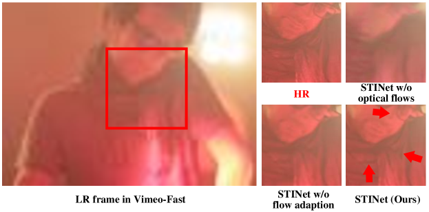
Figure 7: Visual results of the ablation study regarding the adapted optical flows. STINet shows more photo-realistic details. Ground truth is given as HR.

4.4 Ablation study

Table 1 presents the basic ablation study on the proposed ST-FI, ST-LR, ST-GR modules and motion consistency loss, MCL. We use STINet w/o HR to indicate that we only initialize and interpolate LR features in the ST-FI module. The subsequent ST-LR and ST-GR modules are thus degraded to only work on LR features without LR-HR interaction. We observe clear decrease on PSNR and SSIM from STINet to STINet w/o HR. Similar observations can be found on STINet w/o LR where we only use HR features in the main body of the network. The performance decrease of these two variants justify our primary motivation of performing comprehensive LR-HR feature interaction in STVSR.

Next, as shown in Table 1, when we remove ST-LR, ST-GR or MCL from STINet, the performance clearly declines on all datasets. This validates the benefits of ST-LR, ST-GR, and MCL on exploiting spatial-temporal interaction among LR and HR features. Below we detail the ablation study within each module.

Spatial-temporal frame interpolation module (ST-FI).

Adapted optical flows: Referring to Eqn.1, in order to interpolate the intermediate frame feature, we first propose to adapt the original optical flows between two given frames to that from the intermediate frame to given frames. We evaluate the effectiveness of our adapted optical flows in Table 3: STINet w/o optical flows denotes the ST-FI module without using optical flows; STINet w/o flow adaption denotes the ST-FI module using the original optical flows between given frames without adaption, similar to [16]. It can be observed that without using optical flows, the PSNR of STINet significantly decreases by 0.64dB, 0.72dB, 0.57dB, 0.45dB, 0.75dB on five test sets, respectively. Moreover, when using the optical flows yet without flow adaption, the performance of STINet w/o flow adaption is better than that of STINet w/o optical flows but is inferior to STINet. The adapted flows are more accurate to describe motions for the intermediate frame interpolation.

Shareable blocks: next, we evaluate the importance of having shareable residual blocks in ST-FI. Table 4 presents the results using separate residual blocks in the LR and HR interpolation branches (five residual blocks each), i.e. ST-FI w/o share. We can observe that the PSNR decreases by 0.29dB, 0.32dB, 0.20dB, 0.18dB, 0.32dB on five test sets, respectively. This demonstrates that the shareable blocks between LR and HR features are beneficial to encode mutual and complementary information between them and thus help improve the interpolation performance.

Figure. 7 shows some qualitative results for the ablation study of ST-FI. Compared to other variants, STINet reconstructs the scarf with sharper edges and less motion blurs.

Spatial-temporal local refinement module (ST-LR). In ST-LR, we learn two sets of offsets that have the same temporal stamp but different spatial resolutions and we introduce an interaction subnet (Inet) to enable their interaction. First, if we only predict one set of offsets $s^{L}$ (or $s^{H}$) from LR (or HR) features and use it for the local feature alignment in both LR and HR branches, the performance will decrease. We denote the variant by ST-LR w/o $s^{H}$(or ST-LR w/o $s^{L}$) in Table 4. We can observe that both $s^{L}$ and $s^{H}$ contribute to ST-LR; e.g. in Vid4, our STINet shows a decrease of PNSR by -0.10dB and -0.16dB without $s^{L}$ and $s^{H}$, respectively.

Next, we verify the benefits of designing Inet in the ST-LR module. In Table 4, ST-LR w/o Inet denotes ST-LR without Inet such that the learned offsets are directly fed into their respective DCN layers. The performance decreases substantially on all datasets after removing the Inet.

Above results show that the corresponding offsets learned from LR and HR features contain complementary information, and it is essential to interact them for better local feature refinement.

Table 5: Ablation study on the proposed MCL.

	Vid4		Vimeo-Fast		Vimeo-Medium		Vimeo-Slow		Adobe240
Method	PSNR	SSIM	PSNR	SSIM	PSNR	SSIM	PSNR	SSIM	PSNR	SSIM
MCL w/o $l_{abs}$	26.72	0.8044	37.28	0.9444	35.77	0.9376	33.93	0.9170	30.64	0.8751
MCL w/o $l_{rel}$	26.63	0.8039	37.17	0.9443	35.72	0.9366	33.88	0.9167	30.60	0.8747
MCL w/ $l_{abs-AJ}$	26.74	0.8047	37.40	0.9465	35.86	0.9387	34.01	0.9171	30.68	0.8759
MCL w/ $l_{abs-L1}$	26.73	0.8045	37.34	0.9450	35.82	0.9382	33.96	0.9175	30.68	0.8760
MCL w/ $l_{rel-SC}$	26.70	0.8038	37.33	0.9444	35.80	0.9381	33.92	0.9169	30.62	0.8753
MCL (STINet)	26.79	0.8049	37.43	0.9465	35.87	0.9390	34.04	0.9180	30.75	0.8769

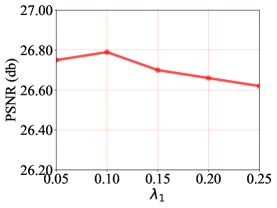
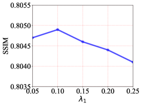
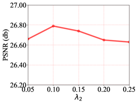
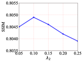
Figure 8: The effect of different loss weights ($\lambda_{1}$ and $\lambda_{2}$) in our loss function. The results are reported on the Vid4 dataset.

Table 6: Results of adding key components of STINet to TMNet [13].

	Vid4		Vimeo-Fast		Vimeo-Medium		Vimeo-Slow		Adobe240
Method	PSNR	SSIM	PSNR	SSIM	PSNR	SSIM	PSNR	SSIM	PSNR	SSIM
TMNet	26.43	0.8016	37.04	0.9435	35.60	0.9380	33.51	0.9159	30.59	0.8760
TMNet w/ HR	26.67	0.8033	37.29	0.9450	35.81	0.9382	33.77	0.9168	30.70	0.8765
TMNet w/ MCL	26.64	0.8029	27.20	0.9439	35.69	0.9385	33.59	0.9163	30.68	0.8762
TMNet w/ ST-GR	26.50	0.8021	37.07	0.9435	35.70	0.9382	33.59	0.9163	30.65	0.8761

Spatial-temporal global refinement module (ST-GR). We investigate the effectiveness of the designed edge attribute in the graph of the ST-GR module. The results are shown in Table 4. We use ST-GR w/o $E^{F}$, ST-GR w/o $E^{P}$ and ST-GR w/o $E^{T}$ to denote the graph without edge attribute $E^{F}$, $E^{P}$ and $E^{T}$ (Sec. 3.4). One can clearly see performance decrease by these variants compared to the original ST-GR (STINet).

Moreover, we compare our ST-GR with the widely used BDConvLSTM layer in previous works [13, 6] for global feature refinement. We denote by ST-GR$\rightarrow$BDCL replacing ST-GR with BDConvLSTM in STINet. Again, the results are inferior to the original STINet. This suggests the superiority of using our ST-GR over BDConvLSTM to globally aggregate spatial-temporal contexts for better feature refinement.

Motion consistency loss (MCL). The motion consistency loss consists of two loss terms, the absolute term $l_{abs}$ (Eqn.2) and the relative term $l_{rel}$ (Eqn.3). To validate their effectiveness, we remove either one and re-train the model. Table 5 shows the results: the PSNR and SSIM decline in all datasets for MCL w/o $l_{abs}$ or $l_{rel}$. Without them, the motions of objects may not be smooth and blurring artifacts may be produced in frames. This is especially the case for the Vimeo-Fast dataset with fast motions. Specifically, we notice that the decline of MCL w/o $l_{rel}$ is bigger than that of MCL w/o $l_{abs}$: for instance, the PSNR decline of the former is 0.16dB while that of the latter is 0.07dB in Vid4. This shows that $l_{rel}$ is more important than $l_{abs}$ in the motion consistency loss.

Next, we present some variants corresponding to $l_{abs}$ and $l_{rel}$, respectively. For $l_{abs}$, referring to Sec. 3.6, we distinguish it from the flow losses in [26, 37]: 1) [26, 37] only supervise flows between adjacent frames; if we do this, denoted by MCL w/ $l_{abs-AJ}$, the performance will be reduced from the original MCL, e.g. in Adobe240, -0.07dB on PSNR and -0.0010 on SSIM. 2) [26, 37] use L1 loss; if we also use L1 loss, denoted by MCL w/ $l_{abs-L1}$, the performance will also be reduced, e.g. in Vid4, -0.06dB on PSNR and -0.0004 on SSIM.

For $l_{rel}$, we design it as a weak constraint rather than a strong one to avoid overfitting. If we instead optimize it upon the exact difference between ${O}_{t-1\rightarrow t}^{pred}-{O}_{t-1\rightarrow t+1}^{pred}$ and ${O}_{t-1\rightarrow t}^{gt}-{O}_{t-1\rightarrow t+1}^{gt}$, denoted by MCL w/ $l_{rel-SC}$ in Table 5, the performance will decrease compared to the original MCL: e.g. the PSNR and SSIM are -0.09dB and -0.0011 on Vid4.

4.5 Parameter variation

We vary the loss weights ($\lambda_{1}$ and $\lambda_{2}$) for the perceptual loss and the proposed MCL in Eqn.4 and report the performance on the Vid4 dataset in Figure. 8. We can observe that the best performance occurs when $\lambda_{1}=0.1$ and $\lambda_{2}=0.1$, which is our default setting.

4.6 Method generalizability

Our proposed components are not only effective in STINet but can also generalize to other methods. We take the state of the art method TMNet [13] as a baseline to add the key components in our STINet. The results are shown in Table 6: 1) we add HR features to the TMNet (denoted as TMNet w/ HR) such that the LR and HR features are respectively refined via two separate branches and finally fused for video reconstruction. Sizeable improvement can be observed upon the original TMNet: i.e. in Vid4, we obtain +0.24dB on PSNR and +0.0017 on SSIM. This validates our idea of exploiting both LR and HR features in the STVSR task. Our STINet further improves upon this idea by introducing spatial-temporal interaction between LR and HR features. 2) We add MCL to TMNet (denoted by TMNet w/ MCL) and also observe sizeable improvement: e.g. in Vid4, 26.64dB on PSNR and 0.8029 on SSIM. 3) We replace the BDConvLSTM layers in TMNet with our ST-GR module for global refinement (denoted by TMNet w/ ST-GR), the performance can be improved: e.g. in Adobe240, 30.65dB on PSNR and 0.8761 on SSIM. These results demonstrate the good generalizability of our proposed components for the STVSR task.

5 Conclusion

In this paper, we propose a spatial-temporal feature interaction network (STINet) for STVSR. Our main contribution is the facilitation of spatial-temporal information interaction among LR and HR features of different frames. Specifically, we introduce the ST-FI module for LR and HR feature interpolation, and the ST-LR module to capture motion cues between features of each frame and its neighbors for local refinement. Moreover, the ST-GR module is presented to perform spatial-temporal information passing and exchanging over the whole feature sequence for global refinement. Last, the proposed motion consistency loss can reinforce STINet to maintain motion continuity among reconstructed frames. Experiments on three datasets demonstrated the effectiveness and superiority of STINet over state of the art. In our future work, we plan to further improve the inference speed of STINet to achieve real-time STVSR.

References

- Kang et al. [2020] J. Kang, Y. Jo, S. W. Oh, P. Vajda, S. J. Kim, Deep Space-Time Video Upsampling Networks, in: ECCV, 2020.
- Shechtman et al. [2002] E. Shechtman, Y. Caspi, M. Irani, Increasing Space-Time Resolution in Video, in: ECCV, 2002.
- Shechtman and Caspi [2005] E. Shechtman, Y. Caspi, Space-time super-resolution, IEEE Transactions on Pattern Analysis and Machine Intelligence 27 (2005) 531–545.
- Shahar et al. [2011] O. Shahar, A. Faktor, M. Irani, Space-time super-resolution from a single video, in: CVPR, 2011.
- Mudenagudi et al. [2011] U. Mudenagudi, S. Banerjee, P. K. Kalra, Space-Time Super-Resolution Using Graph-Cut Optimization, IEEE Transactions on Pattern Analysis and Machine Intelligence 33 (2011) 995–1008.
- Xiang et al. [2020] X. Xiang, Y. Tian, Y. Zhang, Y. Fu, J. P. Allebach, C. Xu, Zooming Slow-Mo: Fast and Accurate One-Stage Space-Time Video Super-Resolution, in: CVPR, 2020.
- Bao et al. [2019] W. Bao, W.-S. Lai, C. Ma, X. Zhang, Z. Gao, M.-H. Yang, Depth-Aware Video Frame Interpolation, in: CVPR, 2019.
- Park et al. [2021] M. Park, H. G. Kim, S. Lee, Y. M. Ro, Robust Video Frame Interpolation With Exceptional Motion Map, IEEE Transactions on Circuits and Systems for Video Technology 31 (2021) 754–764.
- Shen et al. [2021] W. Shen, W. Bao, G. Zhai, L. Chen, X. Min, Z. Gao, Video Frame Interpolation and Enhancement via Pyramid Recurrent Framework, IEEE Transactions on Image Processing 30 (2021) 277–292.
- Song et al. [2021] H. Song, W. Xu, D. Liu, B. Liu, Q. Liu, D. N. Metaxas, Multi-Stage Feature Fusion Network for Video Super-Resolution, IEEE Transactions on Image Processing 30 (2021) 2923–2934.
- Yue et al. [2021] Z. Yue, S. Ding, S. Yang, H. Yang, Z. Li, Y. Zhang, Y. Li, Deep Super-Resolution Network for rPPG Information Recovery and Noncontact Heart Rate Estimation, IEEE Transactions on Instrumentation and Measurement 70 (2021) 1–11.
- Lai et al. [2020] Q. Lai, Y. Nie, H. Sun, Q. Xu, Z. Zhang, M. Xiao, Video super-resolution via pre-frame constrained and deep-feature enhanced sparse reconstruction, Pattern Recognition 100 (2020) 107139.
- Xu et al. [2021] G. Xu, J. Xu, Z. Li, L. Wang, X. Sun, M.-M. Cheng, Temporal Modulation Network for Controllable Space-Time Video Super-Resolution, in: CVPR, 2021.
- Geng et al. [2022] Z. Geng, L. Liang, T. Ding, I. Zharkov, RSTT: Real-time Spatial Temporal Transformer for Space-Time Video Super-Resolution, in: CVPR, 2022.
- Cao et al. [2022] J. Cao, J. Liang, K. Zhang, W. Wang, Q. Wang, Y. Zhang, H. Tang, L. Van Gool, Towards Interpretable Video Super-Resolution via Alternating Optimization, in: ECCV, 2022.
- Haris et al. [2020] M. Haris, G. Shakhnarovich, N. Ukita, Space-Time-Aware Multi-Resolution Video Enhancement, in: CVPR, 2020.
- Shi et al. [2021] Z. Shi, X. Liu, C. Li, L. Dai, J. Chen, T. N. Davidson, J. Zhao, Learning for Unconstrained Space-Time Video Super-Resolution, IEEE Transactions on Broadcasting (2021) 1–14.
- Liu and Sun [2011] C. Liu, D. Sun, A Bayesian approach to adaptive video super resolution, in: CVPR, 2011.
- Xue et al. [2019] T. Xue, B. Chen, J. Wu, D. Wei, W. T. Freeman, Video Enhancement with Task-Oriented Flow, International Journal of Computer Vision 127 (2019) 1106–1125.
- Su et al. [2017] S. Su, M. Delbracio, J. Wang, G. Sapiro, W. Heidrich, O. Wang, Deep Video Deblurring for Hand-Held Cameras, in: CVPR, 2017.
- Lee et al. [2020] H. Lee, T. Kim, T.-y. Chung, D. Pak, Y. Ban, S. Lee, AdaCoF: Adaptive Collaboration of Flows for Video Frame Interpolation, in: CVPR, 2020.
- Shi et al. [2022] Z. Shi, X. Liu, K. Shi, L. Dai, J. Chen, Video Frame Interpolation via Generalized Deformable Convolution, IEEE Transactions on Multimedia 24 (2022) 426–439.
- Jiang et al. [2018] H. Jiang, D. Sun, V. Jampani, M.-H. Yang, E. Learned-Miller, J. Kautz, Super SloMo: High Quality Estimation of Multiple Intermediate Frames for Video Interpolation, in: CVPR, 2018.
- Niklaus and Liu [2018] S. Niklaus, F. Liu, Context-Aware Synthesis for Video Frame Interpolation, in: CVPR, 2018.
- Yan et al. [2021] B. Yan, W. Tan, C. Lin, L. Shen, Fine-Grained Motion Estimation for Video Frame Interpolation, IEEE Transactions on Broadcasting 67 (2021) 174–184.
- Huang et al. [2021] Z. Huang, T. Zhang, W. Heng, B. Shi, S. Zhou, RIFE: Real-Time Intermediate Flow Estimation for Video Frame Interpolation, arXiv preprint arXiv:2011.06294 (2021).
- Tao et al. [2017] X. Tao, H. Gao, R. Liao, J. Wang, J. Jia, Detail-Revealing Deep Video Super-Resolution, in: ICCV, 2017.
- Yi et al. [2020] P. Yi, Z. Wang, K. Jiang, Z. Shao, J. Ma, Multi-Temporal Ultra Dense Memory Network for Video Super-Resolution, IEEE Transactions on Circuits and Systems for Video Technology 30 (2020) 2503–2516.
- Haris et al. [2019] M. Haris, G. Shakhnarovich, N. Ukita, Recurrent Back-Projection Network for Video Super-Resolution, in: CVPR, 2019.
- Jo et al. [2018] Y. Jo, S. W. Oh, J. Kang, S. J. Kim, Deep Video Super-Resolution Network Using Dynamic Upsampling Filters Without Explicit Motion Compensation, in: CVPR, 2018.
- Zhang et al. [2021] D. Zhang, J. Shao, Z. Liang, X. Liu, H. T. Shen, Multi-Branch Networks for Video Super-Resolution With Dynamic Reconstruction Strategy, IEEE Transactions on Circuits and Systems for Video Technology 31 (2021) 3954–3966.
- Huang et al. [2018] Y. Huang, W. Wang, L. Wang, Video Super-Resolution via Bidirectional Recurrent Convolutional Networks, IEEE Transactions on Pattern Analysis and Machine Intelligence 40 (2018) 1015–1028.
- Lucas et al. [2019] A. Lucas, S. Lopez-Tapia, R. Molina, A. K. Katsaggelos, Generative Adversarial Networks and Perceptual Losses for Video Super-Resolution, IEEE Transactions on Image Processing 28 (2019) 3312–3327.
- Tarasiewicz et al. [2021] T. Tarasiewicz, J. Nalepa, M. Kawulok, A Graph Neural Network For Multiple-Image Super-Resolution, in: ICIP, 2021.
- Chen et al. [2022] Z. Chen, Y. Chen, J. Liu, X. Xu, V. Goel, Z. Wang, H. Shi, X. Wang, VideoINR: Learning Video Implicit Neural Representation for Continuous Space-Time Super-Resolution, in: CVPR, 2022.
- Hu et al. [2022] M. Hu, K. Jiang, L. Liao, J. Xiao, J. Jiang, Z. Wang, Spatial-Temporal Space Hand-in-Hand: Spatial-Temporal Video Super-Resolution via Cycle-Projected Mutual Learning, in: CVPR, 2022.
- Zhou et al. [2021] C. Zhou, Z. Lu, L. Li, Q. Yan, J.-H. Xue, How Video Super-Resolution and Frame Interpolation Mutually Benefit, in: ACM Multimedia, 2021.
- Tian et al. [2020] Y. Tian, Y. Zhang, Y. Fu, C. Xu, TDAN: Temporally-Deformable Alignment Network for Video Super-Resolution, in: CVPR, 2020.
- Dai et al. [2017] J. Dai, H. Qi, Y. Xiong, Y. Li, G. Zhang, H. Hu, Y. Wei, Deformable Convolutional Networks, in: ICCV, 2017.
- Haris et al. [2018] M. Haris, G. Shakhnarovich, N. Ukita, Deep Back-Projection Networks for Super-Resolution, in: CVPR, 2018.
- Shi et al. [2016] W. Shi, J. Caballero, F. Huszar, J. Totz, A. P. Aitken, R. Bishop, D. Rueckert, Z. Wang, Real-Time Single Image and Video Super-Resolution Using an Efficient Sub-Pixel Convolutional Neural Network, in: CVPR, 2016.
- Wang et al. [2021] T. Wang, S. Liu, Y. Tian, K. Li, M.-H. Yang, Video Matting via Consistency-Regularized Graph Neural Networks, in: ICCV, 2021.
- Dai et al. [2021] P. Dai, R. Weng, W. Choi, C. Zhang, Z. He, W. Ding, Learning a Proposal Classifier for Multiple Object Tracking, in: CVPR, 2021.
- Hamilton et al. [2017] W. Hamilton, Z. Ying, J. Leskovec, Inductive Representation Learning on Large Graphs, in: NIPS, 2017.
- Simonyan and Zisserman [2015] K. Simonyan, A. Zisserman, Very Deep Convolutional Networks for Large-Scale Image Recognition, in: ICLR, 2015.
- He et al. [2015] K. He, X. Zhang, S. Ren, J. Sun, Delving Deep into Rectifiers: Surpassing Human-Level Performance on ImageNet Classification, in: ICCV, 2015.
- Kingma and Ba [2017] D. P. Kingma, J. Ba, Adam: A Method for Stochastic Optimization, in: ICLR, 2017.
- Wang et al. [2004] Z. Wang, A. Bovik, H. Sheikh, E. Simoncelli, Image Quality Assessment: From Error Visibility to Structural Similarity, IEEE Transactions on Image Processing 13 (2004) 600–612.
- Niklaus et al. [2017] S. Niklaus, L. Mai, F. Liu, Video Frame Interpolation via Adaptive Separable Convolution, in: ICCV, 2017.
- Zhang et al. [2018] Y. Zhang, K. Li, K. Li, L. Wang, B. Zhong, Y. Fu, Image Super-Resolution Using Very Deep Residual Channel Attention Networks, in: ECCV, 2018.
- Wang et al. [2019] X. Wang, K. C. Chan, K. Yu, C. Dong, C. C. Loy, EDVR: Video Restoration With Enhanced Deformable Convolutional Networks, in: CVPR Workshops, 2019.
- Park et al. [2020] J. Park, K. Ko, C. Lee, C.-S. Kim, BMBC: Bilateral Motion Estimation with Bilateral Cost Volume for Video Interpolation, in: ECCV, 2020.
- Liu et al. [2022] C. Liu, H. Yang, J. Fu, X. Qian, Learning Trajectory-Aware Transformer for Video Super-Resolution, in: CVPR, 2022.
- Isobe et al. [2022] T. Isobe, X. Jia, X. Tao, C. Li, R. Li, Y. Shi, J. Mu, H. Lu, Y.-W. Tai, Look Back and Forth: Video Super-Resolution with Explicit Temporal Difference Modeling, in: CVPR, 2022.
- Park et al. [2021] J. Park, C. Lee, C.-S. Kim, Asymmetric Bilateral Motion Estimation for Video Frame Interpolation, in: ICCV, 2021.