Online Learning with Off-Policy Feedback

Abstract

We study the problem of online learning in adversarial bandit problems under a partial observability model called off-policy feedback. In this sequential decision making problem, the learner cannot directly observe its rewards, but instead sees the ones obtained by another unknown policy run in parallel (behavior policy). Instead of a standard exploration-exploitation dilemma, the learner has to face another challenge in this setting: due to limited observations outside of their control, the learner may not be able to estimate the value of each policy equally well. To address this issue, we propose a set of algorithms that guarantee regret bounds that scale with a natural notion of mismatch between any comparator policy and the behavior policy, achieving improved performance against comparators that are well-covered by the observations. We also provide an extension to the setting of adversarial linear contextual bandits, and verify the theoretical guarantees via a set of experiments. Our key algorithmic idea is adapting the notion of pessimistic reward estimators that has been recently popular in the context of off-policy reinforcement learning.

1 Introduction

Off-policy learning is one of the most fundamental concepts in reinforcement learning, concerned with the problem of learning an optimal behavior policy given sample observations generated by a (most likely suboptimal) behavior policy. This setting comes with a unique set of challenges arising from the fact that the learning agent has no influence over the observed data, and thus classical methods for reducing uncertainty via exploration do not directly apply. The inability to explore may suggest that off-policy learning is better approached as a simple “pure exploitation” problem and can be potentially solved by a greedy approach—however, more thought reveals that an effective learning method should also attempt to account for the uncertainty of the random observations. Indeed, the problem setting comes with multiple layers of uncertainty: one layer being the potentially random choices made by the behavior policy, and another being the randomness in the observed rewards. In the present paper, we study a setting where the two uncertainties can be decoupled and addressed individually: the setting of online learning against an adversarial sequence of rewards, with off-policy feedback revealed by a stationary random policy.

The setting we study lies in the intersection of two distinct paradigms of sequential decision making: adversarial online learning and off-policy reinforcement learning. Concretely, we study a sequential decision making problem where in each round, the learner has to pick one of $K$ actions in order to maximize its total rewards. The sequence of reward assignments to actions are decided by an adversary, with each reward function determined the moment before the learner selects its action. The unique feature of the setting is that the learner does not get to observe its reward. However, the learner does observe the reward of another action that has been randomly sampled according to a behavior policy that remains fixed during the learning process. The goal of the learner is then to gain nearly as much reward as the best fixed comparator policy.

While there is indeed no exploration-exploitation dilemma that the learner has to address in this setting, some precaution in selecting the actions is still needed due to the potentially malicious choices of the adversary. Another, perhaps bigger, challenge is that the learner has to estimate the rewards of its own actions from observations made by another policy. The rewards of actions that are observed less frequently are obviously more difficult to estimate. It is thus a sensible requirement to have better performance guarantees against actions that have been more frequently played than against less well-understood actions. More generally, we aim to obtain guarantees that depend on how well the comparator policy is “covered” by the behavior policy.

Our main contribution is an online learning algorithm that guarantees a total expected regret against any comparator policy $\pi^{*}$ that is of order $\sqrt{n}\sum_{a}\frac{\pi^{*}(a)}{\pi_{B}(a)}$, where $\pi_{B}$ is the behavior policy. Our method makes use of a slight pessimistic adjustment to the classic importance-weighted reward estimators commonly used in the adversarial bandit literature. We refer to the problem-dependent factor appearing in the bound as the coverage ratio and denote it by $C(\pi^{*};\pi_{B})$. The coverage ratio quantifies the overlap between the comparator and behavior policies: it is of order $K$ when the two policies closely match each other, but it blows up quickly as the two policies start to differ. Notably, our bounds can be orders of magnitude better than what one would obtain by adapting a standard adversarial bandit method without adjustments. For instance, a naïve analysis of the classic Exp3 method only gives a regret bound of order $\sqrt{n/\min_{a}\pi_{B}(a)}$ against all comparator policies—even against ones that are actually well covered by the behavior policy. Besides providing theoretical results, we also confirm empirically that the performance of these two methods can be quite different, and in particular that Exp3 can indeed fail to take advantage of the comparator policy being poorly covered by the behavior policy.

Our contributions are most easily interpreted in the broader context of online learning under partial monitoring, which generally considers situations where the observations made by the learner are decoupled from its rewards (Rustichini, 1999; Bartók et al., 2014; Lattimore and Szepesvári, 2019). In a general partial monitoring scenario, the learner receives an observation that depends on its action but may be insufficient to reconstruct the obtained reward. A well-studied special case of partial monitoring problems is online learning with feedback graphs (Mannor and Shamir, 2011; Alon et al., 2015, 2017; Kocák et al., 2014, 2016). In this setting, the set of observations associated with each action are given by a directed graph whose nodes are the actions: if actions $a$ and $a^{\prime}$ are connected with an arc pointing from $a$ to $a^{\prime}$, the learner observes the reward of action $a$ when it plays action $a^{\prime}$. The graph may not have self-loops for every action, which allows the possibility that the learner will not observe its own reward. Clearly, our setting can be embedded in this class of problems by considering a sequence of randomly generated star graphs where the action taken by the behavior policy is connected with all other actions. However, the graph does not contain self-loops which renders all existing methods for this problem unsuitable for our problem. In this sense, our contribution sheds some new light on the hardness of learning with feedback graphs without self-loops, and can potentially inspire future work in this domain.

Another line of work closely related to ours is the literature on offline reinforcement learning, where the learner cannot interact with the environment and has instead only access to a fixed dataset gathered by a behavior policy (Levine et al., 2020). In this context, the idea of of employing some form of pessimism has been extremely popular in the last few years, and pessimism has been purported to come with many desirable properties (Jin et al., 2021; Buckman et al., 2021; Uehara and Sun, 2021; Rashidinejad et al., 2021; Xie et al., 2021). One of these is that pessimistic offline RL methods can overcome the typical limitation of requiring the behavior policy to sufficiently explore the whole state-action space, which many previous results suffer from (Antos et al., 2008; Munos and Szepesvári, 2008; Chen and Jiang, 2019; Xie and Jiang, 2021). This assumption is very strong and often not verified in practice. However, a series of recent works show that, via an appropriate use of pessimism, it is possible to obtain bounds which scale with the coverage with respect to a comparator policy, instead of the whole state-action space. Many of these results are surveyed in the work of Xiao et al. (2021), who show that pessimistic policies are minimax optimal with respect to a special objective that weighs problem instances with a notion of inherent difficulty of estimating the value of the optimal policy. On the other hand, they show that without such weighting, pessimism is in fact only one of many possible heuristics that are all minimax optimal when considering the natural version of the optimization objective. This highlights that pessimism may not necessarily play a special role in offline optimization, and that the quest to understand the complexity of offline reinforcement learning is far from being over.

While our results definitely do not settle the debate of whether or not pessimism is the best way to deal with off-policy observations, they do provide some new insights. Most importantly, our findings highlight that pessimism remains an effective method for obtaining comparator-dependent guarantees. Such guarantees have attracted quite some interest in the literature on online learning with fully observable outcomes Chaudhuri et al. (2009); Koolen (2013); Luo and Schapire (2015); Koolen and van Erven (2015); Orabona and Pál (2016); Cutkosky and Orabona (2018). One common building block of parameter-free methods in this context is the Prod algorithm of Cesa-Bianchi et al. (2007), used, for instance, in the algorithm designs of Sani et al. (2014); Gaillard et al. (2014); Koolen and van Erven (2015). Interestingly, our analysis also leans heavily on the tools developed by Cesa-Bianchi et al. (2007). When it comes to the bandit setting, comparator-dependent results are apparently much more sparse and in fact we are only aware of the work of Lattimore (2015) that studies the possibility of guaranteeing better performance against certain comparators. As for our specific problem, we are not aware of any existing method that would be able to guarantee meaningful instance-dependent performance bounds.

Notation.

We denote the set of probability distributions over a set $\mathcal{S}$ as $\Delta_{\mathcal{S}}$. We denote the scalar product of $x,y\in^{d}$ as $\left\langle x,y\right\rangle$ and use $\|\cdot\|_{2}$ to denote the Euclidean norm. For a positive semi-definite matrix $A\in^{d\times d}$, we write $\lambda_{\min}(A)$ and $\operatorname{Tr}{(A)}$ to denote respectively its smallest eigenvalue and its trace. Finally, we use the conventions that $\prod_{k=i}^{j}=1$ and $\sum_{k=i}^{j}=0$ when $j<i$.

2 Preliminaries

We study an $n$-rounds sequential-decision game between a learner (who has a finite set of actions $\mathcal{A}$) and an adversary, where the following steps are repeated in each round $t\in[n]$:

1. The adversary picks a reward function $r_{t}:\mathcal{A}\to[0,1]$, mapping each action to a nonnegative numerical reward,

2. an action $A_{t}\in\mathcal{A}$ is selected by the learner,

3. another action $A^{B}_{t}\in\mathcal{A}$ is selected according to a fixed behavior policy $\pi_{B}$,

4. the learner gains reward $R_{t}=r_{t}(A_{t})$ and observes $R^{B}_{t}=r_{t}(A^{B}_{t})$ along with $A^{B}_{t}$.

Notably, the learner does not get to observe its own reward $R_{t}$ but has to make do with the reward $R^{B}_{t}$ gained by the behavior policy. We allow the adversary to be adaptive in the sense of being able to take into account all past actions of the learner and the behavior policy when selecting the reward function. Also, the learner is allowed to use randomization for selecting its action. Precisely, we will denote the history of interactions up to the end of round $t$ by $\mathcal{F}_{t}=\sigma\left(r_{t},A^{B}_{t},A_{t},\dots,r_{1},A^{B}_{1},A_{1}\right)$, and respectively denote conditional expectations and probabilities with respect to the induced filtration by $\mathbb{E}_{t}\left[\cdot\right]=\mathbb{E}\left[\left.\cdot\right|\mathcal{F}_{t-1}\right]$ and $\mathbb{P}_{t}\left[\cdot\right]=\mathbb{P}\left[\left.\cdot\right|\mathcal{F}_{t-1}\right]$. With this notation, we define the policy of the learner as $\pi_{t}(a)=\mathbb{P}_{t}\left[A_{t}=a\right]$ for all actions $a\in\mathcal{A}$.

The objective of the learner is to minimize the regret, with respect to any time-invariant comparator policy $\pi^{*}\in\Delta_{\mathcal{A}}$, defined as

$$\mathcal{R}(\pi^{*})=\sum^{n}_{t=1}\sum_{a}\bigl{(}\pi^{*}(a)-\pi_{t}(a)\bigr{)}r_{t}(a).$$ (1)

In particular we will be interested in providing bounds on $\mathbb{E}[\mathcal{R}(\pi^{*})]$, where the expectation integrates over all the randomness involved in selecting the random actions $A_{t}$ and $A^{B}_{t}$ and the reward functions $r_{t}$. In words, the expected regret measures the expected gap between the total rewards gained by the learner and the amount gained by a fixed comparator policy $\pi^{*}$.

The most common definition of regret compares the learner’s performance to the optimal policy $\pi^{*}$ that selects the action $a^{*}=\mathop{\mbox{ arg\,max}}_{a}\sum_{t=1}^{n}r_{t}(a)$. However, it is easy to see that this comparator strategy may be unsuitable for measuring performance in the setting we consider. Specifically, it is unreasonable to expect strong guarantees against the optimal policy when the behavior policy selects the optimal actions very rarely. Specifically, the adversary can take advantage of the behavior policy covering the action space only partially, and hide the best rewards among the least-frequently sampled actions. In the most extreme case, the behavior policy may not select some actions at all, which clearly makes it impossible for the learner to compete with the optimal policy. Thus, we aim to achieve regret guarantees that scale with the level of mismatch between the behavior and comparator policies, capturing the intuition that comparator strategies that are well covered by the data should be easier to compete with. Concretely, we will define the coverage ratio between $\pi^{*}$ and $\pi_{B}$ as

$$C(\pi^{*};\pi_{B})=\sum_{a}\frac{\pi^{*}(a)}{\pi_{B}(a)},$$ (2)

and aim to provide regret bounds that scale with this quantity. The intuitive significance of this coverage ratio is that it roughly captures the hardness of estimating the value of the comparator policy $\pi^{*}$ using only data from $\pi_{B}$. Indeed, a simple argument reveals that the estimation error of the total reward of any given action $a$ scales as $\sqrt{n/\pi_{B}(a)}$ in the worst case. Thus, we set out to prove regret guarantees against each comparator $\pi^{*}$ that scale proportionally to the worst-case estimation error of order $\sqrt{C(\pi^{*};\pi_{B})n}$.

3 Algorithm and main results

This section presents our main contributions: a set of algorithms for online off-policy learning and their comparator-dependent performance guarantees that scale with the coverage ratio between the comparator policy and the behavior policy. For the sake of clarity of exposition, we first describe our approach in a relatively simple setting where the number of actions is finite and the behavior policy is known. We then extend the algorithm to be able to deal with unknown behavior policies in Section 3.2 and to linear contextual bandit problems in Section 3.3.

Algorithm 1 Exp3-IX for Off-Policy Learning

  Input: learning rate $\eta$, IX parameters $\left(\gamma_{t}\right)_{t=1}^{n}$

  for $t\leftarrow 1,\dots,n$ do

     compute $w_{t}(a)=\exp(\eta\sum_{k=1}^{t-1}\widetilde{r}_{k}(a))\quad\forall a\in\mathcal{A}$

     play $A_{t}$ according to $\pi_{t}(\cdot)=w_{t}(\cdot)/\sum_{a\in\mathcal{A}}w_{t}(a)$

     observe $A^{B}_{t}$ and $R^{B}_{t}$

     compute $\widetilde{r}_{t}(A^{B}_{t})=R^{B}_{t}/\left(\pi_{B}(A^{B}_{t})+\gamma_{t}\right)$

  end for

3.1 Known behavior policy

Let us first consider the case where the learner has full prior knowledge of $\pi_{B}$. The algorithm we propose is an adaptation of the Exp3-IX algorithm first proposed by Kocák et al. (2014) and later analyzed more generally by Neu (2015). At each time-step $t$ the algorithm computes the weights

$$w_{1}(a) =1,$$

$$w_{t}(a) =w_{t-1}(a)e^{\eta\,\widetilde{r}_{t-1}(a)}=\exp\left(\eta\sum_{k=1}^{t-1}\widetilde{r}_{k}(a)\right),$$

and the normalization factors $W_{t}=\sum_{a}w_{t}(a)$, and uses them to draw the action $A_{t}$ according to $\pi_{t}(a)=\frac{w_{t}(a)}{W_{t}}$. Here, $\eta$ is a positive learning-rate parameter and $\widetilde{r}$ is the Implicit eXploration (IX) estimate of the reward function $r_{t}$, modified to use the rewards obtained by the behavior policy $\pi_{B}$, since the learner cannot see its own rewards:

$$\widetilde{r}_{t}(a)=\frac{R^{B}_{t}\mathbbm{1}\{A^{B}_{t}=a\}}{\pi_{B}(a)+\gamma_{t}}=\frac{r_{t}(a)\mathbbm{1}\{A^{B}_{t}=a\}}{\pi_{B}(a)+\gamma_{t}},$$ (3)

where $\gamma_{t}\geq 0$ is an appropriately chosen parameter. The full algorithm is shown as Algorithm 1 .

When setting $\gamma_{t}=0$, $\widetilde{r}_{t}$ is clearly an unbiased estimator of $r_{t}$ since $\mathbb{E}_{t}\left[\mathbbm{1}\{A^{B}_{t}=a\}\right]=\pi_{B}(a)$. Otherwise, for $\gamma_{t}>0$, the estimator is biased towards zero which can be seen as a pessimistic bias in the sense that it underestimates the true rewards: $\mathbb{E}_{t}\left[\widetilde{r}_{t}(a)\right]\leq r_{t}(a)$. As our results below show, this property is crucially important to achieve our goal to obtain performance guarantees that scale with the mismatch between $\pi^{*}$ and $\pi_{B}$ . In particular, our main result regarding this method is the following:

Theorem 3.1.

For any comparator policy $\pi^{*}$, the expected regret of Exp3-IX initialized with any positive learning rate $\eta$ and $\gamma_{t}=\frac{\eta}{2}$, is bounded as

$$\mathbb{E}[\mathcal{R}(\pi^{*})]\leq\frac{\log K}{\eta}+\frac{\eta}{2}\sum^{n}_{t=1}\sum_{a}\frac{r_{t}(a)\pi^{*}(a)}{\pi_{B}(a)+\frac{\eta}{2}}.$$ (4)

Setting the learning rate to $\eta=\sqrt{\frac{\log K}{n}}$ and to $\eta=\sqrt{\frac{\log K}{C(\pi^{*};\pi_{B})n}}$ respectively gives

$$\mathbb{E}[\mathcal{R}(\pi^{*})] \leq\sqrt{n\log{K}}\left(1+\frac{1}{2}C(\pi^{*};\pi_{B})\right)$$ (5)

$$\mathbb{E}[\mathcal{R}(\pi^{*})] \leq\sqrt{2C(\pi^{*};\pi_{B})n\log{K}}.$$ (6)

The proof is based on a set of small but important changes made to the standard Exp3 analysis originally due to Auer et al. (2002), and is deferred to Section 4. The bound above successfully achieves our goal of guaranteeing better regret against comparator policies that are well-covered by the behavior policy. In particular, the first bound of Equation (5) provides a bound that holds uniformly for all behavior policies without requiring prior commitment to any coverage level, whereas the second bound guarantees improved guarantees against policies with a given coverage level at the price of using a learning-rate parameter that is specific to the desired coverage. Notably, the coverage ratio is of the order $K$ when the comparator policy closely matches the behavior policy, but the actual bound of Equation (4) can be much smaller when there are many actions that the behavior policy selects with probability much smaller than $\gamma$.

It is worthwhile to compare this result with what one would obtain by a straightforward adaptation of a standard adversarial bandit algorithm like Exp3 (Auer et al., 2002)—which essentially corresponds to our algorithm with the choice $\gamma=0$. A standard calculation shows that the regret of this strategy can be upper bounded by

$$\mathbb{E}[\mathcal{R}(\pi^{*})]\leq\frac{\log K}{\eta}+\eta\sum^{n}_{t=1}\sum_{a}\mathbb{E}\left[\frac{\pi_{t}(a)}{\pi_{B}(a)}\right].$$

Notice that the right-hand side of this bound does not depend on the comparator policy, which suggests that this method is not quite suitable for achieving our goal. Even worse, the only way to bound the second term in the bound seems to be by $n/\min_{a}\pi_{B}(a)$, which scales inversely with the coverage of the least well-covered action. A pessimistic interpretation of this argument suggests that Exp3 may have huge regret when some actions are not covered appropriately. A more charitable reading is that Exp3 may not be able to take advantage of situations where the comparator policy is well-covered by the behavior policy. We set out to understand this phenomenon empirically in Section 5.

3.2 Unknown behavior policy

In the previous section we assumed to have full prior knowledge of the behavior policy $\pi_{B}$ in order to compute our reward estimator $\widehat{r}_{t}$. In this section, we show that this is not an inherent limitation of our technique and that it can be easily addressed by using a simple plugin estimator $\widehat{\pi}_{t}$ of the behavior policy, which is then used in the definition of $\widetilde{r}_{t}$:

$$\widehat{\pi}_{1}(\cdot) =0,\qquad\qquad\widehat{\pi}_{t}(a)=\frac{1}{t-1}\sum_{k=1}^{t-1}\mathbbm{1}\{A^{B}_{k}=a\},$$ (7)

$$\widetilde{r}_{t}(a) =\frac{r_{t}(a)\mathbbm{1}\{A^{B}_{t}=a\}}{\widehat{\pi}_{t}(a)+\gamma_{t}}.$$ (8)

We then feed these reward estimates to the exponential-weights procedure described in the previous section. As the following theorem shows, the resulting algorithm satisfies essentially the same regret bound as the method that has full knowledge of $\pi_{B}$.

Theorem 3.2.

For any comparator policy $\pi^{*}$, the expected regret of Exp3-IX with learning rate $\eta=\sqrt{\log(K)/n}$ and parameter sequence $\gamma_{1}=1+\frac{\eta}{2}$, $\gamma_{t}=\frac{\eta}{2}+\sqrt{\log(K(t-1)^{2})/(2t-2)}$, and estimates as in Equation (7), is bounded as

$$\mathbb{E}\left[\mathcal{R}(\pi^{*})\right]=\mathcal{O}\left(C(\pi^{*};\pi_{B})\sqrt{n\log(Kn)}\right).$$ (9)

The parameter tuning achieving the above bound is similar to what is used in the previous theorem, and does not require the learner to have any problem-specific information that would be difficult to acquire. Details are relegated to Appendix B along with the proof of the theorem.

3.3 Linear contextual bandits

We now switch gears and provide an extension to a significantly more advanced setup: that of adversarial linear contextual bandits, first studied by Neu and Olkhovskaya (2020). In each round $t$ of this sequential game, the learner first observes a context $X_{t}$ before making its decision, and the reward function $r_{t}$ is assumed to be an adversarially chosen function of the context $X_{t}$ and the action $A_{t}$ taken by the learner. In particular, the adversary chooses a reward vector $\theta_{t}\in\mathbb{R}^{d}$ at each step, which determines the rewards for each context-action pair as $r_{t}(x,a)=\left\langle\theta_{t},\varphi(x,a)\right\rangle$, where $\varphi:\mathcal{X}\times\mathcal{A}\to\mathbb{R}^{d}$ is a feature map known to both the learner and the adversary. We assume that the contexts live in an abstract space $\mathcal{X}$ and are drawn i.i.d. according to a fixed probability distribution for all $t$. On the other hand, the adversary has full freedom in choosing the reward functions, as long as it only depends on past observations and in particular does not depend on $X_{t}$ or $A_{t}$. The only restriction we put on the adversary is that we continue to require the rewards to be in the interval $[0,1]$. Moreover, as in the previous section the learner is not allowed to see its own rewards, but only the ones of an other policy $\pi_{B}$ running in parallel. In this setting, a policy $\pi$ is a mapping from contexts to probability distributions over the space of actions.

The objective of the learner is to minimize the regret defined with respect to any time-invariant comparator policy $\pi^{*}:\mathcal{X}\rightarrow\Delta_{\mathcal{A}}$ as:

$$\mathcal{R}(\pi^{*})=\sum^{n}_{t=1}\sum_{a}\left(\pi^{*}(a|X_{t})-\pi_{t}(a|X_{t})\right)r_{t}(X_{t},a).$$

Our algorithm for this setting is a combination of the context-wise exponential weights method proposed by Neu and Olkhovskaya (2020) with the ideas developed in the previous section. The algorithm design is complicated by the fact that the implicit exploration estimator is not very straightforward to extend to this setting, which necessitates an alternative (but closely related) approach. In particular, we will define an unbiased estimator of the reward vector $\theta_{t}$ and feed the resulting reward estimates to calculate policy updates via the Prod update rule proposed by Cesa-Bianchi et al. (2007) (see also Cesa-Bianchi and Lugosi (2006), Section 2.7).

Concretely, following the algorithm design of Neu and Olkhovskaya (2020), we define the matrix $\overline{V}(\pi)=\mathbb{E}_{t}\left[\sum_{a}\pi(a|X_{t})\varphi(X_{t},a)\varphi(X_{t},a)^{\mathsf{\scriptscriptstyle T}}\right]$ and the estimator

$$\widehat{\theta}_{t}=\left(\overline{V}(\pi_{B})\right)^{-1}\varphi(X_{t},A^{B}_{t})R^{B}_{t}.$$ (10)

Since $\varphi(X_{t},A^{B}_{t})R^{B}_{t}=\varphi(X_{t},A^{B}_{t})\varphi(X_{t},A^{B}_{t})^{\mathsf{\scriptscriptstyle T}}\theta_{t}$, it is easy to see that $\widehat{\theta}_{t}$ is an unbiased estimator of $\theta_{t}$. These estimators are then used to update a set of weights $w_{t}$ defined for each context-action pair as

$$w_{t}(x,a)=\prod_{k=1}^{t-1}(1+\eta\langle\widehat{\theta}_{k},\varphi(x,a)\rangle),$$

$$W_{t}(x)=\sum_{a}w_{t}(x,a),$$

and the policy is then given as $\pi_{t}(a|x)=\frac{w_{t}(x,a)}{W_{t}(x)}$. Notice that the policy can be easily implemented without explicitly keeping track of the weights for all $(x,a)$ pairs, as they are well-defined through the sequence of reward-estimate vectors $\widehat{\theta}_{1},\dots,\widehat{\theta}_{t-1}$. For simplicity, we assume that the matrix $\overline{V}(\pi_{B})$ is known for the learner and has uniformly lower-bounded eigenvalues so that its inverse exists. Following the naming convention of Neu and Olkhovskaya (2020), we call the resulting algorithm LinProd and show its pseudocode in Algorithm 2.

Algorithm 2 LinProd for off-policy learning

  Input: learning rate $\eta$

  for $t\leftarrow 1,\dots,n$ do

     observe $X_{t}$

     compute $w_{t}(X_{t},\cdot)=\prod_{k=1}^{t-1}\bigl{(}1+\eta\langle\widehat{\theta}_{k},\varphi(X_{t},\cdot)\rangle\bigr{)}$

     draw $A_{t}$ from $\pi_{t}(\cdot|X_{t})=w_{t}(X_{t},\cdot)/\sum_{a}w_{t}(X_{t},a)$

     observe $R^{B}_{t}$ and $\varphi(X_{t},A^{B}_{t})$

     compute $\widehat{\theta}_{t}$ as in Equation 10

  end for

Similarly to the previous sections, we are aiming for a comparator-dependent performance guarantee that depends on the mismatch of the comparator and the behavior policy. However, this quantity is not straightforward to define in the case that we consider, due to the fact that we consider a potentially infinite space of contexts. In particular, the natural idea of considering $\mathbb{E}\left[\sum_{a}\frac{\pi^{*}(a|X_{t})}{\pi_{B}(a|X_{t})}\right]$ as a measure of mismatch is problematic as it can blow up when there exists even a tiny set of contexts where the two policies have no overlap. Intuitively, it should be possible to estimate the reward vector even when there are states where the policies pick different actions, as long as they are aligned in the feature space in an appropriate sense. To make this intuition formal, we will consider the following alternative notion of feature coverage ratio:

$$C_{\varphi}(\pi^{*};\pi_{B})=\operatorname{Tr}\Big{[}{\left(\overline{V}(\pi_{B})\right)^{-1}\,\overline{V}(\pi^{*})}\Big{]}.$$ (11)

This notion of coverage appropriately measures the extent to which the feature vectors $\varphi(X_{t},A_{t}^{*})$ generated by the comparator policy line up with the features excited by the behavior policy. Similar distribution-mismatch measures are common in the offline RL literature, and in particular the results of Jin et al. (2021) are stated in terms of the same quantity. The following theorem gives a performance guarantee stated in terms of this measure of distribution mismatch.

Theorem 3.3.

Let $\eta$ be any positive learning rate and suppose that it is small enough so that $\lambda_{\min}(\overline{V}(\pi_{B}))\geq 2\eta\,\sup_{x,a}\left\|\phi(x,a)\right\|^{2}_{2}$ holds. Then, for any comparator policy $\pi^{*}$ the expected regret of LinProd is upper-bounded by

$$\mathbb{E}\big{[}\mathcal{R}(\pi^{*})\big{]}\leq\frac{\log K}{\eta}+\eta nC_{\varphi}(\pi^{*};\pi_{B}),$$

Setting $\eta=\sqrt{\frac{\log K}{n}}$ and $\eta=\sqrt{\frac{\log K}{C_{\varphi}(\pi^{*};\pi_{B})n}}$ and supposing that $n$ is large enough so that $\eta$ satisfies the condition, the regret can be further bounded respectively as

$$\mathbb{E}[\mathcal{R}(\pi^{*})] \leq\sqrt{n\log K}\left(1+C_{\varphi}(\pi^{*};\pi_{B})\right),$$

$$\mathbb{E}[\mathcal{R}(\pi^{*})] \leq 2\sqrt{C_{\varphi}(\pi^{*};\pi_{B})n\log K}.$$

The bound mirrors the qualities of Theorem 3.1, and in particular it implies good performance when the comparator policy is well-covered by the behavior policy. Under ideal conditions where these policies are close enough, the coverage ratio is of order $d$, which essentially matches the rate proved by Neu and Olkhovskaya (2020) for the case of standard bandit feedback. The bound then degrades as the two policies drift apart.

4 Analysis

This section provides the key ideas required for proving our main results. Due to space restrictions, we will only prove Theorem 3.1 here and defer the proof of the other two theorems to Appendices B and C.

For the analysis, it will be useful to define the unbiased reward estimator $\widehat{r}_{t}(a)=\frac{r_{t}(a)\mathbbm{1}\{A^{B}_{t}=a\}}{\pi_{B}(a)}$, which essentially corresponds to the biased IX estimator $\widetilde{r}_{t}$ when setting $\gamma_{t}=0$. One of the most important properties of the IX estimator that we will repeatedly use is stated in the following inequality:

$$\frac{r_{t}(a)\mathbbm{1}\{A^{B}_{t}=a\}}{\pi_{B}(a)+\gamma_{t}}\leq\frac{1}{2\gamma_{t}}\log\left(1+2\gamma_{t}\widehat{r}_{t}(a)\right).$$ (12)

The result follows from a simple calculation in the proof of Lemma 1 of Neu (2015) that we reproduce in Appendix A.1 for the convenience of the reader. Notably, the term on the right hand side can be thought of as a reward estimator itself. Combining this reward estimator with the exponential weights policy with $\eta=\gamma$ gives rise to the Prod algorithm of Cesa-Bianchi et al. (2007), which is a fact that some of our proofs will implicitly take advantage of. This observation also motivates our algorithm design for the contextual bandit setting in Section 3.3.

The proof of Theorem 3.1

The proof builds on the classical analysis of exponential weights algorithm originally due to Vovk (1990), Littlestone and Warmuth (1994) and Freund and Schapire (1997), and its extension to adversarial bandit problems by Auer et al. (2002). In particular, our starting point is the following lemma that can be proved directly with arguments borrowed from any of these past works:

Lemma 4.1.

$$\sum^{n}_{t=1}\sum_{a}\pi^{*}(a)\widetilde{r}_{t}(a)\leq\frac{\log K}{\eta}$$

$$\qquad+\frac{1}{\eta}\sum^{n}_{t=1}\log\sum_{a}\pi_{t}(a)\exp\left(\eta\widetilde{r}_{t}(a)\right).$$

We include the proof for the sake of completeness in Appendix A.2. To proceed, notice that the above bound can be combined with Equation (12) to obtain

$$\sum^{n}_{t=1}\sum_{a}\pi^{*}(a)\widetilde{r}_{t}(a)\leq\frac{\log K}{\eta}$$ (13)

$$\qquad+\frac{1}{\eta}\sum^{n}_{t=1}\log\sum_{a}\pi_{t}(a)\exp\left(\frac{\eta}{2\gamma}\log\left(1+2\gamma\,\widehat{r}_{t}(a)\right)\right)$$

$$\quad=\frac{\log K}{\eta}+\frac{1}{\eta}\sum^{n}_{t=1}\log\sum_{a}\pi_{t}(a)\left(1+\eta\widehat{r}_{t}(a)\right)$$

$$\quad\leq\frac{\log K}{\eta}+\sum^{n}_{t=1}\sum_{a}\pi_{t}(a)\widehat{r}_{t}(a),$$

where we used the choice $\gamma=\eta/2$ in the second line and the inequality $\log(1+x)\leq x$ that holds for all $x>-1$ in the last line.

It remains to relate the two sums in the above expression to the total reward of the learner and the comparator policy. To this end, we first notice that for any given action $a$, we have

$$\mathbb{E}_{t}\left[\widetilde{r}_{t}(a)\right] =\mathbb{E}_{t}\left[\frac{r_{t}(a)\mathbbm{1}\{A^{B}_{t}=a\}}{\pi_{B}(a)+\gamma}\right]$$ (14)

$$=\frac{r_{t}(a)\pi_{B}(a)}{\pi_{B}(a)+\gamma}=r_{t}(a)-\frac{\gamma r_{t}(a)}{\pi_{B}(a)+\gamma}.$$

Via the tower rule of expectation, this implies

$$\mathbb{E}\left[\sum^{n}_{t=1}\sum_{a}\pi^{*}(a)\widetilde{r}_{t}(a)\right]$$

$$=\mathbb{E}\left[\sum^{n}_{t=1}\sum_{a}\pi^{*}(a)r_{t}(a)\right]-\gamma\sum^{n}_{t=1}\sum_{a}\frac{\pi^{*}(a)r_{t}(a)}{\pi_{B}(a)+\gamma}.$$

Similarly, since $\mathbb{E}_{t}\left[\widehat{r}_{t}(a)\right]=r_{t}(a)$, we also have

$$\mathbb{E}\left[\sum^{n}_{t=1}\sum_{a}\pi_{t}(a)\widehat{r}_{t}(a)\right]=\mathbb{E}\left[\sum^{n}_{t=1}\sum_{a}\pi_{t}(a)r_{t}(a)\right].$$

Putting these two facts together with Equation (13), we obtain the result claimed in the theorem.

5 Empirical Results

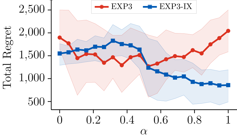
Figure 1: Total regret after $1000$ steps for different values of the interpolation parameter $\alpha$. Thick lines represent the mean regret over $100$ independent runs, while the shaded area represents the interval between the $25\%$ and $75\%$ quantiles.

This section provides a set of experiments to illustrate our main results, and in particular to verify if Exp3-IX can indeed take advantage of behavior policies that are well-aligned with the comparator. In particular, we compare the performance of Exp3-IX (Algorithm 1) and Exp3 in the the following experiment. We instantiate a $100$-armed bandit, with Bernoulli rewards for all arms. By default, all rewards have mean $0.5$. However, for the first half of the game ($t\leq n/2$), we change the mean reward of the last arm to $0.8$, and for the remaining half, the mean of the first arm to $1$. This means that arm $100$ is the best for the first half of the game, but eventually gets outperformed by arm $1$. We set the number of rounds $n$ to $10000$, the learning rate $\eta$ of both algorithms to the recommended $\sqrt{\log(K)/n}$ and $\gamma_{t}=\eta/2$.

We repeat the game for a range of behavior policies defined for each $\alpha$ as $\pi_{B,\alpha}(i)\propto(1-\alpha)\frac{i}{K}+\alpha(1-\frac{i-1}{K})$, for $i\in[0,\dots,K]$, where $\alpha$ varies from $0$ to $1$. Hence, $\alpha$ closer to $1$ means the behavior policy puts large probability mass on the first action, which we use as the comparator in our experiment. We plot the results of the experiment on Figure 1 The results clearly match the intuitions that one can derive from our performance guarantees. First, recall that a naïve analysis of Exp3 suggests that its regret may scale as $\sqrt{n/\min_{a}\pi_{B}(a)}$ in the worst case. Our empirical results show that this crude analysis is not entirely off track: the regret of Exp3 indeed deteriorates as $\min_{a}\pi_{B}(a)$ approaches $0$ at the two extremes $\alpha=0$ and $\alpha=1$. In particular, Exp3 fails to take advantage of the favorable case where the optimal policy is well-covered and performs similarly as in the case where the optimal policy is not covered at all. In comparison, Exp3-IX performs significantly better when the comparator policy is well covered, as predicted by our theory. Other experiments on the same problem with alternative parametrizations gave qualitatively similar results.

6 Conclusion

We introduced a new online learning setting where the learner is only allowed to observe off-policy feedback generated by a fixed behavior policy. We have proposed an algorithm with comparator-dependent regret bounds of order $C(\pi^{*};\pi_{B})\sqrt{n}$, depending on a naturally defined coverage ratio parameter $C(\pi^{*};\pi_{B})$ that characterizes the mismatch between the behavior and the comparator policies. Many questions remain open regarding the potential tightness of this result. First, we have shown that the bounds can be improved to $O(\sqrt{C(\pi^{*};\pi_{B})n})$, if one wishes to restrict their attention to comparators whose coverage level is at a fixed level $C(\pi^{*};\pi_{B})$. However, the tuning required for achieving this result depends on the desired coverage level. It is an interesting open problem to find out if this requirement can be relaxed, and bounds of order $\sqrt{C(\pi^{*};\pi_{B})n}$ can be simultaneously achieved for all comparators $\pi^{*}$ by a single algorithm. We conjecture that this question can be addressed by a careful adaptation of existing techniques for adaptive online learning, and in particular we believe that adapting the methodology of Koolen and van Erven (2015) should be especially suitable for achieving this goal.

Questions regarding the best achievable performances for our newly defined problem are even more exciting. As an adaptation of the results of Xiao et al. (2021) show via an online-to-batch reduction, the minimax regret of any algorithm for this setting has to scale as $\sqrt{n/\min_{a}\pi_{B}(a)}$, suggesting that our naïve adaptation of Exp3 is already minimax optimal. In our view, this makes it all the more interesting to identify characteristics of individual problem instances that make faster learning possible, and we believe that comparator-dependent regret bounds scaling with the coverage ratio are only one of many possible flavors of adaptive performance guarantees. One concrete question that we are particularly interested in is a better understanding of the “Pareto regret frontier” of achievable regrets, roughly corresponding to the set of comparator-dependent regret bounds that are achievable by any algorithm. Clearly, the bounds we achieve are just singular elements of this set. We conjecture that bounds of order $\sqrt{C(\pi^{*};\pi_{B})n}$ are indeed on the regret frontier. Whether this is indeed true or if there are other distinguished entries on the Pareto frontier with desirable properties remains to be seen. All in all, our results highlight that off-policy learning is a field of study that’s ripe with open questions that can be interesting for the online learning community that is typically very keen on instance-dependent analysis.

A more ambitious question for future research is if our techniques can be extended to more challenging settings, and especially online learning in Markov decision processes (Even-Dar et al., 2009; neu10o-ssp; Neu et al., 2014). We think that an extension to this setting would be particularly valuable, given the recent flurry of interest in offline reinforcement learning. In this context, we could potentially exploit the unique feature of our algorithm design that, unlike all other methods, it does not rely on explicit uncertainty quantification for calculating its pessimistic updates. This could mean a major advantage over traditional off-policy RL methods that rely on uncertainty quantification to build confidence sets over abstract objects (like the entire transition function of the Markov process), which is a notoriously hard problem, especially in the infinite-horizon setting. In contrast, as our results in Section 3.3 highlight, the pessimistic nature of our method is realized through an update rule that is slightly more conservative than the standard exponential-weights update rule. We believe that this insight can be very useful for developing new methods for offline RL, even more so since they appear to be directly compatible with the primal-dual off-policy learning methods of Nachum et al. (2019a, b); Uehara et al. (2020).

Appendix A Omitted details from the proof of Theorem 3.1

A.1 Proof of the bound of Equation (12)

This proof is extracted from the proof of Lemma 1 of Neu [2015]. Let $c\in\mathbb{R}_{+}$ be any non-negative constant. Then,

$$\frac{r_{t}(a)\mathbbm{1}\{A_{t}=a\}}{\pi_{B}(a)+c}\leq\frac{r_{t}(a)\mathbbm{1}\{A_{t}=a\}}{\pi_{B}(a)+c\,r_{t}(a)}=\frac{\mathbbm{1}\{A_{t}=a\}}{2c}\cdot\frac{{2c\,r_{t}(a)}/{\pi_{B}(a)}}{1+{c\,r_{t}(a)}/{\pi_{B}(a)}}\leq\frac{1}{2c}\log(1+2c\,\widehat{r}_{t}(a))$$

where the first step follows from $r_{t}(a)\in[0,1]$ and the last one from the inequality $\frac{x}{1+x/2}\leq\log(1+x)$, which holds for all $x\geq 0$.

A.2 The proof of Lemma 4.1

We study the evolution of the potential function $\frac{1}{\eta}\log\frac{W_{n+1}}{W_{1}}$. On the one hand, we have for any action $\bar{a}$ that

$$\frac{1}{\eta}\log\frac{W_{n+1}}{W_{1}}=\frac{1}{\eta}\log\left(\frac{1}{K}\sum_{a}w_{n+1}(a)\right)\geq\frac{1}{\eta}\log\left(\frac{1}{K}\,w_{n+1}(\bar{a})\right)=\sum^{n}_{t=1}\widetilde{r}_{t}(a)-\frac{\log K}{\eta}.$$ (15)

Multiplying this bound with $\pi^{*}(\bar{a})$ and summing up over actions gives the lower bound

$$\frac{1}{\eta}\log\frac{W_{n+1}}{W_{1}}\geq\sum^{n}_{t=1}\sum_{a}\pi^{*}(a)\widetilde{r}_{t}(a)-\frac{1}{\eta}\log K.$$ (16)

On the other hand, the potential can be rewritten as follows:

$$\frac{1}{\eta}\log\frac{W_{n+1}}{W_{1}} =\frac{1}{\eta}\sum^{n}_{t=1}\log\frac{W_{t+1}}{W_{t}}=\frac{1}{\eta}\sum^{n}_{t=1}\log\frac{\sum_{a}w_{t}(a)e^{\eta\widetilde{r}_{t}(a)}}{W_{t}}=\frac{1}{\eta}\sum^{n}_{t=1}\log\sum_{a}\pi_{t}(a)e^{\eta\widetilde{r}_{t}(a)}.$$

Putting the two expressions together concludes the proof.

Appendix B The proof of Theorem 3.2

In this proof, we have to face the added challenge of having to account for the possible inaccuracy of our estimator of $\pi_{B}$. To this end, we define a sequence of “good events” under which the policy estimate is well-concentrated and analyze the regret under this event and its complement, using that the good event should hold with high probability. Concretely, we define the failure probability $\delta_{t}\in(0,1)$, the tolerance parameter $\varepsilon_{t}$, and the $t$-th good event as follows:

$$\varepsilon_{1}=1\,,\quad\varepsilon_{t}=\sqrt{\frac{\log(K/\delta_{t})}{2(t-1)}} E_{t}=\big{\{}|\widehat{\pi}_{t}(a)-\pi_{B}(a)|\leq\varepsilon_{t}\,\,(\forall a\in\mathcal{A})\big{\}}.$$ (17)

An application of Hoeffding’s inequality shows that $E_{t}$ holds with probability at least $1-\delta_{t}$. Now, setting $\gamma_{t}=\varepsilon_{t}+\eta/2$, we can observe that under event $E_{t}$, we have

$$\widetilde{r}_{t}(a)=\frac{r_{t}(a)\mathbbm{1}\{A^{B}_{t}=a\}}{\widehat{\pi}_{t}+\gamma_{t}}\leq\frac{r_{t}(a)\mathbbm{1}\{A^{B}_{t}=a\}}{\pi_{B}(a)+\eta/2}\leq\frac{1}{\eta}\log(1+\eta\widehat{r}_{t}(a)).$$ (18)

We proceed by noticing that the bound of Lemma 4.1 continues to apply, and that we can bound the term appearing on the right-hand side as follows:

$$\mathbb{E}_{t}\left[\frac{1}{\eta}\log\sum_{a}\pi_{t}(a)\exp\left(\eta\widetilde{r}_{t}(a)\right)\right]\leq\mathbbm{1}\{E_{t}\}\mathbb{E}_{t}\left[\frac{1}{\eta}\log\sum_{a}\pi_{t}(a)\exp\left(\eta\widetilde{r}_{t}(a)\right)\right]+\mathbbm{1}\{\overline{E}_{t}\}\frac{2}{\eta}$$

$$\qquad\qquad\leq\mathbbm{1}\{E_{t}\}\mathbb{E}_{t}\left[\sum_{a}\pi_{t}(a)\widehat{r}_{t}(a)\right]+\mathbbm{1}\{\overline{E}_{t}\}\frac{2}{\eta}\leq\sum_{a}\pi_{t}(a)r_{t}(a)+\mathbbm{1}\{\overline{E}_{t}\}\frac{2}{\eta},$$

where in the first line we used that $e^{\eta\widetilde{r}_{t}(a)}\leq e^{\eta/\gamma_{t}}\leq e^{2}$ and in the second line we used the bound of Equation (18), the fact that $E_{t}$ is $\mathcal{F}_{t-1}$-measurable, that $\mathbb{E}_{t}\left[\widehat{r}_{t}(a)\right]=r_{t}(a)$, and finally upper bounded the indicator $\mathbbm{1}\{E_{t}\}$ by one. Taking marginal expectations and summing up for all $t$, we get

$$\mathbb{E}\left[\frac{1}{\eta}\sum_{t=1}^{n}\log\sum_{a}\pi_{t}(a)\exp\left(\eta\widetilde{r}_{t}(a)\right)\right]\leq\mathbb{E}\left[\sum^{n}_{t=1}\sum_{a}\pi_{t}(a)r_{t}(a)\right]+\frac{2}{\eta}\sum^{n}_{t=1}\delta_{t},$$

where we used $\mathbb{E}\left[\mathbbm{1}\{\overline{E}_{t}\}\right]\leq\delta_{t}$.

It thus remains to relate the term on the left-hand side of the bound of Lemma 4.1. To do this, we similarly write

$$\mathbb{E}_{t}\left[\widetilde{r}_{t}(a)\right] \geq\mathbbm{1}\{E_{t}\}\mathbb{E}_{t}\left[\widetilde{r}_{t}(a)\right]=\mathbbm{1}\{E_{t}\}\mathbb{E}_{t}\left[\frac{r_{t}(a)\mathbbm{1}\{A^{B}_{t}=a\}}{\widehat{\pi}_{t}(a)+\gamma_{t}}\right]$$

$$\geq\mathbbm{1}\{E_{t}\}\cdot\frac{r_{t}(a)\pi_{B}(a)}{\pi_{B}(a)+\varepsilon_{t}+\gamma_{t}}\geq\mathbbm{1}\{E_{t}\}r_{t}(a)-\frac{\varepsilon_{t}+\gamma_{t}}{\pi_{B}(a)},$$

where in the first inequality we exploited that $\widetilde{r}_{t}(a)$ is nonnegative, in the second one we used that $E_{t}$ is $\mathcal{F}_{t-1}$-measurable and the defining property of the good event, and in the last one we simplified some expressions. Thus, we have

$$\mathbb{E}\left[\sum^{n}_{t=1}\sum_{a}\pi^{*}(a)r_{t}(a)\right] \leq\mathbb{E}\left[\sum^{n}_{t=1}\sum_{a}\pi^{*}(a)\left(\widetilde{r}_{t}(a)+(1-\mathbbm{1}\{E_{t}\})r_{t}(a)+\frac{\varepsilon_{t}+\gamma_{t}}{\pi_{B}(a)}\right)\right]$$

$$=\mathbb{E}\left[\sum^{n}_{t=1}\sum_{a}\pi^{*}(a)\widetilde{r}_{t}(a)\right]+\sum^{n}_{t=1}\delta_{t}+\sum_{a}\frac{\pi^{*}(a)}{\pi_{B}(a)}\sum^{n}_{t=1}\left(2\varepsilon_{t}+\frac{\eta}{2}\right),$$

where in the last line we recalled that $\gamma_{t}=\varepsilon_{t}+\eta/2$. Putting the two bounds together, we arrive to

$$\mathbb{E}\left[\sum^{n}_{t=1}\sum_{a}\left(\pi^{*}(a)r_{t}(a)-\pi_{t}(a)r_{t}(a)\right)\right] \leq\frac{\log K}{\eta}+\left(1+\frac{2}{\eta}\right)\sum^{n}_{t=1}\delta_{t}+\left(\frac{\eta n}{2}+2\sum^{n}_{t=1}\varepsilon_{t}\right)\sum_{a}\frac{\pi^{*}(a)}{\pi_{b}(a)}$$

Finally, we set $\delta_{1}=0\,,\,\delta_{t}=(t-1)^{-2}$ so that we have $\sum^{n}_{t=1}\delta_{t}=\pi^{2}/6\leq 2$ and we can write

$$\sum^{n}_{t=1}\varepsilon_{t}=1+\sum_{t=1}^{n-1}\sqrt{\frac{\log(Kt^{2})}{2t}}\leq 2\sqrt{n\log(Kn)},$$

where we also used the standard upper bound $\sum_{t=1}^{n}1/\sqrt{t}\leq 2\sqrt{n}$. Putting everything together, we finally get

$$\mathbb{E}\left[\sum^{n}_{t=1}\sum_{a}\left(\pi^{*}(a)r_{t}(a)-\pi_{t}(a)r_{t}(a)\right)\right]\leq\frac{16+\log K}{\eta}+\left(\frac{\eta n}{2}+2\sqrt{n\log(Kn)}\right)C(\pi^{*};\pi_{B})+2.$$

Setting $\eta=\sqrt{\frac{\log K}{n}}$ concludes the proof.

Appendix C The proof of Theorem 3.3

The proof combines ideas from the previous two proofs with ideas from Neu and Olkhovskaya [2020] to deal with the contextual aspect of the problem setting. In the following, let $\widehat{r}_{t}(x,a)=\langle\widehat{\theta}_{t},\varphi(x,a)\rangle$. As a starting point, we fix a context $x\in\mathcal{X}$ and define the estimated regret in context $x$ against comparator $\pi^{*}$ as

$$\widehat{\mathcal{R}}(\pi^{*},x)=\sum^{n}_{t=1}\sum_{a}\left(\pi^{*}(a|x)-\pi_{t}(a|x)\right)\widehat{r}_{t}(x,a).$$ (19)

The following lemma gives a bound on the above quantity:

Lemma C.1.

Suppose that $\eta\widehat{r}_{t}(x,a)\geq-1/2$ holds for all $x,a$. Then, for any fixed $x$ and $\pi^{*}$,

$$\widehat{\mathcal{R}}(\pi^{*},x)\leq\frac{\log K}{\eta}+\eta\sum^{n}_{t=1} \sum_{a}\pi^{*}(a|x)\left(\widehat{r}_{t}(x,a)\right)^{2}.$$ (20)

The proof follows from a careful combination of techniques by Cesa-Bianchi et al. [2007] and Neu and Olkhovskaya [2020], and is deferred to Appendix C.2. We proceed by noting that for any fixed $x$, the second term in the bound can be bounded as follows:

$$\begin{split}\mathbb{E}_{t}\left[\left(\widehat{r}_{t}(x,a)\right)^{2}\right]&=\mathbb{E}_{t}\left[\left(R^{B}_{t}\right)^{2}\varphi(x,a)^{\mathsf{\scriptscriptstyle T}}\left(\overline{V}(\pi_{B})\right)^{-1}\varphi(X_{t},A^{B}_{t})\varphi(X_{t},A^{B}_{t})^{\top}\left(\overline{V}(\pi_{B})\right)^{-1}\varphi(x,a)\right]\\ &\leq\varphi(x,a)^{\top}\left(\overline{V}(\pi_{B})\right)^{-1}\overline{V}(\pi_{B})\left(\overline{V}(\pi_{B})\right)^{-1}\varphi(x,a)=\varphi(x,a)^{\mathsf{\scriptscriptstyle T}}\left(\overline{V}(\pi_{B})\right)^{-1}\varphi(x,a)\\ &=\operatorname{Tr}{\Big{(}\left(\overline{V}(\pi_{B})\right)^{-1}\varphi(x,a)\varphi(x,a)^{\mathsf{\scriptscriptstyle T}}\Big{)}},\end{split}$$ (21)

where we have used $R^{B}_{t}\leq 1$ in the inequality. Furthermore, in order to use the lemma, we first need to verify that its precondition is satisfied. To this end, notice that

$$\left|\widehat{r}_{t}(x,a)\right| =\left|R_{t}\phi(x,a)^{\mathsf{\scriptscriptstyle T}}\left(\overline{V}(\pi_{B})\right)^{-1}\phi(X_{t},A_{t}^{b})\right|\leq\frac{\sup_{x,a}\left\|\phi(x,a)\right\|^{2}_{2}}{\lambda_{\min}(\overline{V}(\pi_{B}))},$$

which follows from a straightforward applicaiton of the Cauchy–Schwarz inequality. Thus, the condition on $\eta$ we impose in the theorem guarantees that $\eta|\widehat{r}_{t}(x,a)|\leq 1/2$. Now we are in position to invoke Lemma C.1, albeit with a specific choice for the context $x$. Specifically, we let $X_{0}$ be a “ghost sample” drawn independently from the context distribution for the sake analysis, and apply Lemma C.1 to obtain

$$\widehat{\mathcal{R}}(\pi^{*},X_{0})\leq\frac{\log K}{\eta}+\eta\sum^{n}_{t=1} \sum_{a}\pi^{*}(a|X_{0})\operatorname{Tr}{\Big{(}\left(\overline{V}(\pi_{B})\right)^{-1}\varphi(X_{0},a)\varphi(X_{0},a)^{\mathsf{\scriptscriptstyle T}}\Big{)}}.$$ (22)

Then, a straightforward calculation inspired by the analysis of Neu and Olkhovskaya [2020] shows that the left-hand side is related to the expected regret as

$$\mathbb{E}\left[\widehat{\mathcal{R}}(\pi^{*},X_{0})\right]=\mathbb{E}\left[\sum^{n}_{t=1}\sum_{a}\left(\pi^{*}(a|X_{t})-\pi_{t}(a|X_{t})\right)r_{t}(X_{t},a)\right].$$ (23)

For completeness, we include this calculation in Appendix C.1. The same technique can be used to deal with the term on the right-hand side as follows:

$$\mathbb{E}\left[\sum^{n}_{t=1}\sum_{a}\pi^{*}(a|X_{0})\operatorname{Tr}\Big{(}{\left(\overline{V}(\pi_{B})\right)^{-1}\phi(X_{0},a)\phi(X_{0},a)^{\mathsf{\scriptscriptstyle T}}}\Big{)}\right]$$

$$=\mathbb{E}\left[\sum^{n}_{t=1}\operatorname{Tr}{\Big{(}\left(\overline{V}(\pi_{B})\right)^{-1}\sum_{a}\pi^{*}(a|X_{0})\phi(X_{0},a)\phi(X_{0},a)^{\mathsf{\scriptscriptstyle T}}}\Big{)}\right]$$

$$=\mathbb{E}\left[\sum^{n}_{t=1}\operatorname{Tr}{\Big{(}\left(\overline{V}(\pi_{B})\right)^{-1}\overline{V}(\pi^{*})\Big{)}}\right]=C_{\varphi}(\pi^{*};\pi_{B}).$$

Thus, taking expectations of both sides of Equation (22) and using the above two results concludes the proof. ∎

C.1 The proof of the regret decomposition of Equation (23)

We start by fixing an arbitrary $x$ and defining the following notion of pseudo-regret in context $x$:

$$\mathcal{R}(\pi^{*},x)=\sum^{n}_{t=1}\sum_{a}\left(\pi^{*}(a|x)-\pi_{t}(a|x)\right)r_{t}(x,a).$$

We first note that $\mathbb{E}[\widehat{\mathcal{R}}(\pi^{*},x)]=\mathbb{E}[\mathcal{R}(\pi^{*},x)]$ holds thanks to the unbiasedness of $\widehat{r}_{t}$ and the independence of $\pi_{t}$ and $\widehat{r}_{t}$. In particular, this follows from the following derivation:

$$\mathbb{E}[\widehat{\mathcal{R}}(\pi^{*},x)] =\mathbb{E}\left[\sum^{n}_{t=1}\mathbb{E}_{#1}\Big{[}\sum_{a}\left(\pi^{*}(a|x)-\pi_{t}(a|x)\right)\widehat{r}_{t}(x,a)\Big{]}\right]$$

$$=\mathbb{E}\left[\sum^{n}_{t=1}\sum_{a}\left(\pi^{*}(a|x)-\pi_{t}(a|x)\right)\mathbb{E}_{#1}\Big{[}\widehat{r}_{t}(x,a)\Big{]}\right]$$

$$=\mathbb{E}\left[\sum^{n}_{t=1}\sum_{a}\left(\pi^{*}(a|x)-\pi_{t}(a|x)\right)r_{t}(x,a)\right]=\mathbb{E}[\mathcal{R}(\pi^{*},x)],$$

where we used the tower rule of expectation in the first step, the fact that $\pi_{t}$ is $\mathcal{F}_{t-1}$-measurable in the second step, and the unbiasedness of the reward estimator in the last step. To relate $\mathbb{E}[\mathcal{R}(\pi^{*},x)]$ and the true expected Regret $\mathbb{E}[\mathcal{R}(\pi^{*})]$, we consider the random variable $\mathcal{R}(\pi^{*},X_{0})$ with $X_{0}$ being a ghost sample drawn from the context distribution independently from the history of contexts $(X_{t})_{t=1}^{n}$. Then, we can write the expectation of this random variable as

$$\mathbb{E}[\mathcal{R}(\pi^{*},X_{0})]=\mathbb{E}\left[\sum^{n}_{t=1}\sum_{a}\left(\pi^{*}(a|X_{0})-\pi_{t}(a|X_{0})\right)r_{t}(X_{0},a)\right]$$

$$=\mathbb{E}\left[\sum^{n}_{t=1}\mathbb{E}_{#1}\Big{[}\sum_{a}\left(\pi^{*}(a|X_{0})-\pi_{t}(a|X_{0})\right)r_{t}(X_{0},a)\Big{]}\right]$$

$$=\mathbb{E}\left[\sum^{n}_{t=1}\mathbb{E}_{#1}\Big{[}\sum_{a}\left(\pi^{*}(a|X_{t})-\pi_{t}(a|X_{t})\right)r_{t}(X_{t},a)\Big{]}\right]=\mathbb{E}[\mathcal{R}(\pi^{*})],$$

where the second line uses the tower rule of expectation and the third one the fact that $X_{0}$ is distributed identically with $X_{t}$ given $\mathcal{F}_{t-1}$. This concludes the proof. ∎

C.2 Proof of Lemma C.1

The proof is inspired by the classic Prod analysis of Cesa-Bianchi et al. [2007], and follows from similar arguments as the proof of Lemma 4.1. The main adjustment we need to these proofs is that now we have to include contexts in our derivations. To this end, let us fix one context $x\in\mathcal{X}$ and suppose that the condition of the theorem is satisfied: $\eta\,\widehat{r}_{t}(x,a)\geq-1/2$ for all actions $a\in\mathcal{A}$.

As before, we will study the evolution of the potential function $\frac{1}{\eta}\log\frac{W_{n+1}(x)}{W_{1}(x)}$. For every action $\bar{a}\in\mathcal{A}$ we have:

$$\frac{1}{\eta}\log W_{n+1}(x) =\frac{1}{\eta}\log\sum_{a}\prod_{t=1}^{n}(1+\eta\widehat{r}_{t}(x,a))\geq\frac{1}{\eta}\log\prod_{t=1}^{n}(1+\eta\widehat{r}_{t}(x,\bar{a}))$$

$$=\frac{1}{\eta}\sum^{n}_{t=1}\log(1+\eta\widehat{r}_{t}(x,\bar{a}))\geq\sum^{n}_{t=1}\big{(}\widehat{r}_{t}(x,\bar{a})-\eta\left(\widehat{r}_{t}(x,\bar{a})\right)^{2}\big{)},$$

where we used our condition on the magnitude of the reward estimates twice: once to use $(1-\eta\widehat{r}_{t}(x,a))\geq 0$ in the first line and once when using the elementary inequality $\log(1+z)\geq z-z^{2}$ that holds for all $z\geq-1/2$ in the second line. Moreover, we can upper-bound the potential as

$$\frac{1}{\eta}\log W_{n+1}(x) =\frac{1}{\eta}\log W_{1}+\frac{1}{\eta}\log\prod_{t=1}^{n}\frac{W_{t+1}(x)}{W_{t}(x)}=\frac{\log K}{\eta}+\frac{1}{\eta}\sum^{n}_{t=1}\log\frac{W_{t+1}(x)}{W_{t}(x)}$$

$$=\frac{\log K}{\eta}+\frac{1}{\eta}\sum^{n}_{t=1}\log\sum_{a}\frac{w_{t}(x,a)}{W_{t}(x)}(1+\eta\,\widehat{r}_{t}(x,a)) \big{(}\text{def. of $W_{t+1}$}\big{)}$$

$$=\frac{\log K}{\eta}+\frac{1}{\eta}\sum^{n}_{t=1}\log\sum_{a}\pi_{t}(a|x)(1+\eta\,\widehat{r}_{t}(x,a)) \big{(}\text{def. of $\pi_{t}$}\big{)}$$

$$=\frac{\log K}{\eta}+\frac{1}{\eta}\sum^{n}_{t=1}\log\Big{(}1+\eta\sum_{a}\pi_{t}(a|x)\widehat{r}_{t}(x,a)\Big{)}$$

$$\leq\frac{\log K}{\eta}+\sum^{n}_{t=1}\sum_{a}\pi_{t}(a|x)\widehat{r}_{t}(x,a),$$

where we used the inequality $\log(1+z)\leq z$ that holds for all $z>-1$.

Combining the lower bound and upper bound, we obtain

$$\sum^{n}_{t=1}\Big{(}\widehat{r}_{t}(x,\bar{a})-\sum_{a}\pi_{t}(a|x)\widehat{r}_{t}(x,a)\Big{)}\leq\frac{\log K}{\eta}+\eta\sum^{n}_{t=1}\left(\widehat{r}_{t}(x,\bar{a})\right)^{2}.$$

Multiplying both sides by $\pi^{*}(\bar{a}|x)$ and summing over all actions $\bar{a}\in\mathcal{A}$ yields the desired result. ∎

References

• Alon etย al. (2015) Noga Alon, Nicolรฒ Cesa-Bianchi, Ofer Dekel, and Tomer Koren. Online learning with feedback graphs: Beyond bandits. In COLT, volumeย 40 of JMLR Workshop and Conference Proceedings, pages 23โ€“35. JMLR.org, 2015.
• Alon etย al. (2017) Noga Alon, Nicolรฒ Cesa-Bianchi, Claudio Gentile, Shie Mannor, Yishay Mansour, and Ohad Shamir. Nonstochastic multi-armed bandits with graph-structured feedback. SIAM J. Comput., 46(6):1785โ€“1826, 2017.
• Antos etย al. (2008) Andrรกs Antos, Csaba Szepesvรกri, and Rรฉmi Munos. Learning near-optimal policies with bellman-residual minimization based fitted policy iteration and a single sample path. Mach. Learn., 71(1):89โ€“129, 2008.
• Auer etย al. (2002) Peter Auer, Nicolรฒ Cesa-Bianchi, Yoav Freund, and Robertย E. Schapire. The nonstochastic multiarmed bandit problem. SIAM J. Comput., 32(1):48โ€“77, 2002.
• Bartรณk etย al. (2014) Gรกbor Bartรณk, Deanย P. Foster, Dรกvid Pรกl, Alexander Rakhlin, and Csaba Szepesvรกri. Partial monitoring - classification, regret bounds, and algorithms. Math. Oper. Res., 39(4):967โ€“997, 2014.
• Buckman etย al. (2021) Jacob Buckman, Carles Gelada, and Marcย G. Bellemare. The importance of pessimism in fixed-dataset policy optimization. In ICLR. OpenReview.net, 2021.
• Cesa-Bianchi and Lugosi (2006) Nicolรฒ Cesa-Bianchi and Gรกbor Lugosi. Prediction, learning, and games. Cambridge University Press, 2006.
• Cesa-Bianchi etย al. (2007) Nicolรฒ Cesa-Bianchi, Yishay Mansour, and Gilles Stoltz. Improved second-order bounds for prediction with expert advice. Mach. Learn., 66(2-3):321โ€“352, 2007.
• Chaudhuri etย al. (2009) Kamalika Chaudhuri, Yoav Freund, and Danielย J. Hsu. A parameter-free hedging algorithm. In NeurIPS, pages 297โ€“305. Curran Associates, Inc., 2009.
• Chen and Jiang (2019) Jinglin Chen and Nan Jiang. Information-theoretic considerations in batch reinforcement learning. In ICML, volumeย 97 of Proceedings of Machine Learning Research, pages 1042โ€“1051. PMLR, 2019.
• Cutkosky and Orabona (2018) Ashok Cutkosky and Francesco Orabona. Black-box reductions for parameter-free online learning in banach spaces. In COLT, volumeย 75 of Proceedings of Machine Learning Research, pages 1493โ€“1529. PMLR, 2018.
• Even-Dar etย al. (2009) Eyal Even-Dar, Shamย M. Kakade, and Yishay Mansour. Online Markov decision processes. Math. Oper. Res., 34(3):726โ€“736, 2009.
• Freund and Schapire (1997) Yoav Freund and Robertย E. Schapire. A decision-theoretic generalization of on-line learning and an application to boosting. J. Comput. Syst. Sci., 55(1):119โ€“139, 1997.
• Gaillard etย al. (2014) Pierre Gaillard, Gilles Stoltz, and Tim van Erven. A second-order bound with excess losses. In COLT, volumeย 35 of JMLR Workshop and Conference Proceedings, pages 176โ€“196. JMLR.org, 2014.
• Jin etย al. (2021) Ying Jin, Zhuoran Yang, and Zhaoran Wang. Is pessimism provably efficient for offline RL? In ICML, volume 139 of Proceedings of Machine Learning Research, pages 5084โ€“5096. PMLR, 2021.
• Kocรกk etย al. (2014) Tomรกลก Kocรกk, Gergely Neu, Michal Valko, and Rรฉmi Munos. Efficient learning by implicit exploration in bandit problems with side observations. In NeurIPS, pages 613โ€“621, 2014.
• Kocรกk etย al. (2016) Tomรกลก Kocรกk, Gergely Neu, and Michal Valko. Online learning with noisy side observations. In AISTATS, volumeย 51 of JMLR Workshop and Conference Proceedings, pages 1186โ€“1194. JMLR.org, 2016.
• Koolen (2013) Wouterย M. Koolen. The Pareto regret frontier. In NeurIPS, pages 863โ€“871, 2013.
• Koolen and van Erven (2015) Wouterย M. Koolen and Tim van Erven. Second-order quantile methods for experts and combinatorial games. In COLT, volumeย 40 of JMLR Workshop and Conference Proceedings, pages 1155โ€“1175. JMLR.org, 2015.
• Lattimore (2015) Tor Lattimore. The Pareto regret frontier for bandits. In NeurIPS, pages 208โ€“216, 2015.
• Lattimore and Szepesvรกri (2019) Tor Lattimore and Csaba Szepesvรกri. Cleaning up the neighborhood: A full classification for adversarial partial monitoring. In ALT, volumeย 98 of Proceedings of Machine Learning Research, pages 529โ€“556. PMLR, 2019.
• Levine etย al. (2020) Sergey Levine, Aviral Kumar, George Tucker, and Justin Fu. Offline reinforcement learning: Tutorial, review, and perspectives on open problems. CoRR, abs/2005.01643, 2020.
• Littlestone and Warmuth (1994) Nick Littlestone and Manfredย K. Warmuth. The weighted majority algorithm. Inf. Comput., 108(2):212โ€“261, 1994.
• Luo and Schapire (2015) Haipeng Luo and Robertย E. Schapire. Achieving all with no parameters: Adanormalhedge. In COLT, volumeย 40 of JMLR Workshop and Conference Proceedings, pages 1286โ€“1304. JMLR.org, 2015.
• Mannor and Shamir (2011) Shie Mannor and Ohad Shamir. From bandits to experts: On the value of side-observations. In NeurIPS, pages 684โ€“692, 2011.
• Munos and Szepesvรกri (2008) Rรฉmi Munos and Csaba Szepesvรกri. Finite-time bounds for fitted value iteration. J. Mach. Learn. Res., 9:815โ€“857, 2008.
• Nachum etย al. (2019a) Ofir Nachum, Yinlam Chow, Boย Dai, and Lihong Li. DualDICE: Behavior-agnostic estimation of discounted stationary distribution corrections. pages 2315โ€“2325, 2019a.
• Nachum etย al. (2019b) Ofir Nachum, Boย Dai, Ilya Kostrikov, Yinlam Chow, Lihong Li, and Dale Schuurmans. AlgaeDICE: Policy gradient from arbitrary experience. CoRR, abs/1912.02074, 2019b.
• Neu (2015) Gergely Neu. Explore no more: Improved high-probability regret bounds for non-stochastic bandits. In NeurIPS, pages 3168โ€“3176, 2015.
• Neu and Olkhovskaya (2020) Gergely Neu and Julia Olkhovskaya. Efficient and robust algorithms for adversarial linear contextual bandits. In COLT, volume 125 of Proceedings of Machine Learning Research, pages 3049โ€“3068. PMLR, 2020.
• Neu etย al. (2014) Gergely Neu, Andrรกs Gyรถrgy, Csaba Szepesvรกri, and Andrรกs Antos. Online Markov decision processes under bandit feedback. IEEE Trans. Autom. Control., 59(3):676โ€“691, 2014.
• Orabona and Pรกl (2016) Francesco Orabona and Dรกvid Pรกl. Coin betting and parameter-free online learning. In NeurIPS, pages 577โ€“585, 2016.
• Rashidinejad etย al. (2021) Paria Rashidinejad, Banghua Zhu, Cong Ma, Jiantao Jiao, and Stuart Russell. Bridging offline reinforcement learning and imitation learning: A tale of pessimism. pages 11702โ€“11716, 2021.
• Rustichini (1999) Aldo Rustichini. Minimizing regret: The general case. Games and Economic Behavior, 29(1-2):224โ€“243, 1999.
• Sani etย al. (2014) Amir Sani, Gergely Neu, and Alessandro Lazaric. Exploiting easy data in online optimization. In NeurIPS, pages 810โ€“818, 2014.
• Uehara and Sun (2021) Masatoshi Uehara and Wen Sun. Pessimistic model-based offline reinforcement learning under partial coverage. arXiv preprint arXiv:2107.06226, 2021.
• Uehara etย al. (2020) Masatoshi Uehara, Jiawei Huang, and Nan Jiang. Minimax weight and q-function learning for off-policy evaluation. In ICML, volume 119 of Proceedings of Machine Learning Research, pages 9659โ€“9668. PMLR, 2020.
• Vovk (1990) Vladimirย G. Vovk. Aggregating strategies. In COLT, pages 371โ€“386. Morgan Kaufmann, 1990.
• Xiao etย al. (2021) Chenjun Xiao, Yifan Wu, Jincheng Mei, Boย Dai, Tor Lattimore, Lihong Li, Csaba Szepesvรกri, and Dale Schuurmans. On the optimality of batch policy optimization algorithms. In ICML, volume 139 of Proceedings of Machine Learning Research, pages 11362โ€“11371. PMLR, 2021.
• Xie and Jiang (2021) Tengyang Xie and Nan Jiang. Batch value-function approximation with only realizability. In ICML, volume 139 of Proceedings of Machine Learning Research, pages 11404โ€“11413. PMLR, 2021.
• Xie etย al. (2021) Tengyang Xie, Ching-An Cheng, Nan Jiang, Paul Mineiro, and Alekh Agarwal. Bellman-consistent pessimism for offline reinforcement learning. In NeurIPS, pages 6683โ€“6694, 2021.