MonoIndoor++:Towards Better Practice of Self-Supervised Monocular Depth Estimation for Indoor Environments

Abstract

Self-supervised monocular depth estimation has seen significant progress in recent years, especially in outdoor environments, i.e., autonomous driving scenes. However, depth prediction results are not satisfying in indoor scenes where most of the existing data are captured with hand-held devices. As compared to outdoor environments, estimating depth of monocular videos for indoor environments, using self-supervised methods, results in two additional challenges: (i) the depth range of indoor video sequences varies a lot across different frames, making it difficult for the depth network to induce consistent depth cues for training, whereas the maximum distance in outdoor scenes mostly stays the same as the camera usually sees the sky; (ii) the indoor sequences recorded with handheld devices often contain much more rotational motions, which cause difficulties for the pose network to predict accurate relative camera poses, while the motions of outdoor sequences are pre-dominantly translational, especially for street-scene driving datasets such as KITTI. In this work, we propose a novel framework-MonoIndoor++ by giving special considerations to those challenges and consolidating a set of good practices for improving the performance of self-supervised monocular depth estimation for indoor environments. First, a depth factorization module with transformer-based scale regression network is proposed to estimate a global depth scale factor explicitly, and the predicted scale factor can indicate the maximum depth values. Second, rather than using a single-stage pose estimation strategy as in previous methods, we propose to utilize a residual pose estimation module to estimate relative camera poses across consecutive frames iteratively. Third, to incorporate extensive coordinates guidance for our residual pose estimation module, we propose to perform coordinate convolutional encoding directly over the inputs to pose networks. The proposed method is validated on a variety of benchmark indoor datasets, i.e., EuRoC MAV, NYUv2, ScanNet and 7-Scenes, demonstrating the state-of-the-art performance. In addition, the effectiveness of each module is shown through a carefully conducted ablation study and the good generalization and universality of our trained model is also demonstrated, specifically on ScanNet and 7-Scenes datasets.

I Introduction

Monocular depth estimation has been applied in a variety of 3D perceptual tasks, including autonomous driving, virtual reality (VR), and augmented reality (AR). Estimating the depth map plays an essential role in these applications, in helping to understand environments, plan agents’ motions, reconstruct 3D scenes, etc. Existing supervised depth methods [1, 2] can achieve high performance, but they require the ground-truth depth data during the training which is often expensive and time-consuming to obtain by using depth sensors (e.g., LiDAR). To this end, a number of recent work [3, 4, 5] have been focused on predicting the depth map from a single image using self-supervised manners and they have shown advantages in scenarios where obtaining the ground-truth is not possible. In these self-supervised frameworks, photometric consistency between multiple views from monocular video sequences has been utilized as the main supervision for training models. Specifically, the recent work [5] has achieved significant success in estimating depth that is comparable to that by the supervised methods [6, 2]. For instance, on the KITTI dataset [7], the Monodepth2, proposed by Godard et al.  [5], achieves an absolute relative depth error (AbsRel) of 10.6%, which is not far from the AbsRel of 7.2% by the DORN which is a supervised model proposed by Fu et al.  [2]. However, most of these self-supervised depth prediction methods [3, 4, 5] are only evaluated on datasets of outdoor scenes such as KITTI, leaving their performance opaque for indoor environments. There are certainly ongoing efforts [8, 9, 10] which considers self-supervised monocular depth estimation for indoor environments, but their performance still trail far behind the one on the outdoor datasets by methods such as [3, 4, 5] or the supervised counterparts [2, 11] on indoor datasets. In this paper, we concentrate on estimating the depth map from a single image for indoor environments in a self-supervised manner which only requires monocular video sequences for training.

This paper investigates the performance discrepancies between the indoor and outdoor scenes and takes a step towards examining what makes indoor depth prediction more challenging than the outdoor case. We first identify that the scene depth range of indoor video sequences varies a lot more than in the outdoor and conjecture that this posits more difficulties for the depth network in inducing consistent depth cues across images from monocular videos, resulting in the worse performance on indoor datasets.

Our second observation is that the pose network, which is commonly used in self-supervised methods [4, 5], tends to have large errors in predicting rotational parts of relative camera poses. A similar finding has been presented in  [12] where predicted poses have much higher rotational errors (e.g., 10 times larger) than geometric SLAM [13] even when they use a recurrent neural network as the backbone to model the long-term dependency for pose estimation. We argue that this problem is not prominent on outdoor datasets, i.e., KITTI, because the camera motions therein are mostly translational. However, frequent cameras rotations are inevitable in indoor monocular videos [14, 15] as these datasets are often captured by hand-held cameras or Micro Aerial Vehicle (MAVs). Thus, the inaccurate rotation prediction becomes detrimental to the self-supervised training of a depth model for indoor environments.

Our third conjecture is that the pose network in existing self-supervised methods is potentially suffering from insufficient cues to estimate relative cameras poses between color image pairs in different views. We argue that, rather than simply inducing camera poses based on color information of image pairs, encoding coordinates information can further improve the reliability of pose network in inferring geometric relations among changing views.

We propose MonoIndoor++, a self-supervised monocular depth estimation method tailored for indoor environments, giving special considerations for above problems. Our MonoIndoor++ consists of three novel modules: a depth factorization module, a residual pose estimation module, and a coordinates convolutional encoding module. In the depth factorization module, we factorize the depth map into a global depth scale (for the target image of the current view) and a relative depth map. The depth scale factor is separately predicted by an extra module (named as transformer-based scale regression network) in parallel with the depth network which predicts a relative depth map. In such a way, the depth network has more model plasticity to adapt to the depth scale changes during training. We leverage the recent advances of transformer [16] in designing the scale regression network to predict the depth scale factor. In the residual pose estimation module, we mitigate the issue of inaccurate camera rotation prediction by performing residual pose estimation in addition to an initial large pose prediction. Such a residual approach leads to more accurate computation of the photometric loss [5], which in turn improves model training for the depth prediction. In the coordinates convolutional encoding module, we encode the coordinates information $(x,y)$ explicitly and incorporate them with color information in the residual pose estimation module, expecting to provide additional cues for pose predictions, which further consolidates residual pose estimation model during training.

It should be mentioned that this paper is an extended version of our previous conference paper [17], where we propose an unsupervised learning framework for monocular depth estimation in indoor environments. In this paper, we i) add more technical details of our proposed method; ii) present coordinate convolutional encoding module in the framework for improved performance of monocular depth prediction; iii) make a more clear explanation of our proposed depth factorization module with transformer-based scale network; iv) conduct extensive experiments and ablation studies on public benchmark datasets, i.e., EuRoC MAV [18], NYUv2 [14], ScanNet [19] and 7-Scenes [20], and perform detailed analysis to demonstrate the effectiveness and good generalizability of our proposed framework in this journal paper.

In summary, our contributions are:

• We propose a novel depth factorization module with a transformer-based scale regression network to estimate a global depth scale factor, which helps the depth network adapt to the rapid scale changes for indoor environments during model training.

• We propose a novel residual pose estimation module that mitigates the inaccurate camera rotation prediction issue in the pose network and in turn significantly improves monocular depth estimation performance.

• We incorporate coordinates convolutional encoding in the proposed residual pose estimation module to leverage coordinates cues in inducing relative camera poses.

• We demonstrate the state-of-the-art performance of self-supervised monocular depth prediction on a wide-variety of publicly available indoor datasets, i.e., EuRoC MAV [15], NYUv2 [14], ScanNet [19] and 7-Scenes [20].

The paper is organized as follows: Section II summarizes related published works in the field; then in Section III, we explain our proposed approach for monocular depth estimation in indoor environments, the proposed approach consisting of a depth factorization, a residual pose and a coordinates convolutional encoding modules; and in Section IV, we present experimental results and ablation studies on a variety of benchmark indoor datasets; and lastly a conclusion of our work is discussed in Section V.

II Related Work

Much effort has been expended for the depth estimation in various environments. This paper addresses the self-supervised monocular depth estimation for indoor environments. In this section, we discuss the relevant work of depth estimation using both supervised and self-supervised methods.

II-A Supervised Monocular Depth Estimation

The depth estimation problem was mostly solved by using supervised methods in early research. Saxena et al.  [21] propose the method to regress the depth from a single image by extracting superpixel features and using a Markov Random Field (MRF). Schonberger et al.  [22] present a system for the joint estimation of depth and normal information with photometric and geometric priors. These methods employ traditional geometry-based methods. Eigen et al.  [23] propose the first deep-learning based method for monocular depth estimation using a multi-scale convolutional neural network (CNN). Later on, deep-learning based methods have shown significant progress on monocular depth estimation, specifically with massive ground-truth data during training the networks. One line of following work improves the performance of depth prediction by better network architecture design. Laina et al.  [24] propose an end-to-end fully convolutional architecture by encompassing the residual learning to predict accurate single-view depth maps given monocular images. Bhat et al.  [25] propose a transformer-based architecture block to adaptively estimate depth maps using a number of bins. Another line of work achieves improved depth estimation results by integrating more sophisticated training losses [26, 2, 11, 27, 28, 29]. Besides, a few methods [30, 31] propose to use two networks, one for depth prediction and the other for motion, to mimic geometric Structure-from-Motion (SfM) or Simultaneous Localization and Mapping (SLAM) in a supervised framework. However, ground-truth depth maps with images are used to train these methods and obtaining ground-truth data is often expensive and time-consuming to capture. Some other methods then resort to remedy this problem by generating pseudo ground-truth depth labels with traditional 3D reconstruction methods [32, 33], such as SfM [15] and SLAM [13, 34], or 3D movies [35]. Such methods have better capacity of generalization across different datasets, but cannot necessarily achieve the best performance for the dataset at hand. Some other ongoing efforts explore to improve robustness of supervised monocular depth estimation for zero-shot cross-dataset transfer. Ranftl et al.  [35] propose robust scale-and shift-invariant losses for training the model using data from mixed dataset and testing on zero-shot datasets, and improve it further by integrating vision transformer in network design [36].

II-B Self-Supervised Monocular Depth Estimation

Recently, significant progress has been made in self-supervised depth estimation as it does not require training with the ground-truth data. Garg et al.  [3] propose the first self-supervised method to train a CNN-based model for monocular depth estimation by using color consistency loss between stereo images. Zhou et al.  [4] employ a depth network for depth estimation and a pose network to estimate relative camera poses between temporal frames, and use outputs to construct the photometric loss across temporal frames to train the model. Many follow-up methods then try to propose new training loss terms to improve self-supervision for training models. Godard et al.  [37] incorporate a left-right depth consistency loss for the stereo training. Bian et al.  [38] put forth a temporal depth consistency loss to ensure predicted depth maps of neighbouring frames are consistent. Wang et al.  [39] first observe the diminishing issue of the depth model during training and propose a normalization method to counter this effect. Yin et al.  [40] and Zou et al.  [41] train three networks (i.e., one depth network, one pose network, and one extra flow network) jointly by enforcing cross-task consistency between optical flow and dense depth. Wang et al.  [42] and Zou et al.  [12] explore techniques to improve the performance of pose network and/or the depth network by leveraging recurrent neural networks, such as LSTMs, to model long-term dependency. Tiwari et al.  [43] design a self-improving loop with monocular SLAM and a self-supervised depth model [5] to improve the performance of each one. Among these recent advances, Monodepth2 [5] significantly improves the performance over previous methods via a set of techniques: a per-pixel minimum photometric loss to handle occlusions, an auto-masking method to mask out static pixels, and a multi-scale depth estimation strategy to mitigate the texture-copying issue in depth. Watson et al.  [44] propose to use cost volume in the deep model and a new consistency loss calculated between the a teacher and a student model for self-supervision training. Unlike Monodepth2, this method show its advantages in using multiple frames during the testing. We implement our self-supervised depth estimation framework based on Monodepth2, but make important changes in designing both the depth and the pose networks.

Most of the aforementioned methods are only evaluated on outdoor datasets such as KITTI. Recent ongoing efforts [8, 9, 45] focus on self-supervised depth estimation for indoor environments. Zhou et al.  [8] first observe existing large rotations on most existing indoor datasets, and then use a pre-processing step to handle large rotational motions by removing all the image pairs with “pure rotation” and design an optical-flow based training paradigm using the processed data. Zhao et al.  [9] adopt a geometry-augmented strategy that solves for the depth via two-view triangulation and then uses the triangulated depth as supervision for model training. Bian et al.  [45, 10] theoretically study the reasons behind the unsatisfying deep estimation performance in indoor environments and argue that “the rotation behaves as noise during training”. They propose a rectification step during the data pre-precessing to remove the rotation between consecutive frames and design an auto-rectify network. We have an observation similar to [8, 45] and [10] that large rotations cause difficulties for training the network. However, we take a different strategy. Instead of removing rotations from training data during the data pre-processing, we progressively estimate camera poses in rotations and translations via a novel residual pose module in an end-to-end manner, and we validate the effectiveness of the proposed method in predicting improved depth on a variety of indoor benchmark datasets.

II-C Transformer

We leverage the transformer in designing our scale regression network inspired by the recent advances [46, 47, 16] of the attention mechanism. Self-attention in the transformer was first used successfully in natural lanuage processing (NLP) to model long-term dependencies. Wang et al.  [46] proposes a non-local operations for computer vision tasks. Recently, self-attention and its variants have been widely used in transformer networks for high-level visions tasks such as image classification [16] and semantic segmentation [48, 49].

II-D Coordinates Encoding

Convolutional neural networks (CNNs) have achieved significant success at many tasks, and it can be complemented with specialized layers for certain usage. For instance, detection models like Faster R-CNN [50] make use of layers to compute coordinate transforms. Jaderberg et al.  [51] propose a spatial Transformer module that can be included into a standard CNN model to provide spatial transformation capabilities. Qi et al.  [52, 53] design the PointNet which takes a set of 3D points represented as $(x,y,z)$ coordinates as well as extra color features for 3D classification and segmentation. Recently, coordinates encoding has been widely used in vision transformers [16, 48, 49] and neural radiance fields representations [54, 55, 56]. Vision transformers [16] take 2D images as the input, reshape the image into a sequence of flattened 2D patches and then employ self-attention blocks for image classification, detection and segmentation. Position embeddings are added to the patch embeddings as a standard processing step to retain positional information. Nerf [54] proposes a method which takes a 3D location $(x,y,z)$ and 2D viewing direction $(\theta,\phi)$ as the input for scene synthesis. Unlike in vision transformers where positional encoding is utilized to provide discrete positions of tokens in the sequence, in Nerf, positional functions are used to map continuous input coordinates into a higher dimensional space for high frequency approximations. Liu et al.  [57] define the CoordConv operation to provide extra coordinates information as part of input channels to convolutional filters for the convolutional neural networks. Most of pose networks in monocular depth estimation pipelines [37, 5] simply take two consecutive frames as the input and outputs relative camera poses. We argue such designs infer rotational and translational relations by only focusing on photometric cues, but ignoring explicit coordinates cues. In our work, we leverage coordinates encoding in the proposed residual pose network.

III Method

Figure 1: Overview of the proposed MonoIndoor++. Depth Factorization Module: We use an encoder-decoder based depth network to predict a relative depth map and a transformer-based scale network to estimate a global scale factor. Residual Pose Estimation Module: We use a pose network to predict an initial camera pose of a pair of frames and residual pose network to iteratively predict residual camera poses based on the predicted initial pose. Coordinates Convolutional Encoding: We encode coordinates information along with the concatenated color image pairs as the input to the pose network and residual pose network for predicting relative camera poses.

In this section, we present detailed descriptions of performing self-supervised depth estimation using the proposed MonoIndoor++. Specifically, we first give an overview of the standard framework for the self-supervised depth estimation. Then, we describe three core components including depth factorization, residual pose and coordinates convolution modules, respectively.

III-A Self-Supervised Monocular Depth Estimation

Self-supervised monocular depth estimation is considered as a novel view-synthesis problem which is defined in [4, 5, 12]. This key idea is to train a model to predict the target image from different viewpoints of source images. The image synthesis is achieved by using the depth map as the bridging variable between the depth network and pose network. Both the depth map of the target image and the estimated relative camera pose between a pair of target and source images are required to train such systems. Specifically, the depth network predicts a dense depth map ${D}_{t}$ given a target image $I_{t}$ as the input. The pose network takes a target image $I_{t}$ and a source image $I_{t^{\prime}}$ from another view and estimates a relative camera pose ${T}_{t\rightarrow t^{\prime}}$ from the target to the source. The depth network and pose network are optimized jointly with the photometric reprojection loss which can then be constructed as follows:

$$\mathcal{L}_{A}=\sum_{t^{\prime}}\rho(I_{t},I_{t^{\prime}\rightarrow t}),$$ (1)

and

$$I_{t^{\prime}\rightarrow t}=I_{t^{\prime}}\langle proj({D}_{t},{T}_{t\rightarrow t^{\prime}},K)\rangle,$$ (2)

where $\rho$ denotes the photometric reconstruction error [4, 5]. It is a weighted combination of the L1 and Structured SIMilarity (SSIM) loss defined as

$$\rho(I_{t},I_{t^{\prime}\rightarrow t})=\frac{\alpha}{2}\big{(}1-\texttt{\footnotesize SSIM}(I_{t},I_{t^{\prime}\rightarrow t})\big{)}+(1-\alpha)\|I_{t},I_{t^{\prime}\rightarrow t}\|_{1}.$$ (3)

$I_{t^{\prime}\rightarrow t}$ is the source image warped to the target coordinate frame based on the depth of the target image which is the output from the depth network. $proj()$ is the transformation function to map image coordinated $p_{t}$ from the target image to its $p_{t^{\prime}}$ on the source image following

$$p_{t^{\prime}}\sim K{T}_{t\rightarrow t^{\prime}}{D}_{t}(p_{t})K^{-1}p_{t},$$ (4)

and $\langle\cdot\rangle$ is the bilinear sampling operator which is locally sub-differentiable.

In addition, an edge-ware smoothness term is normally employed during training which can be written as

$$\mathcal{L}_{s}=|\partial_{x}d^{\ast}_{t}|e^{-|\partial_{x}I_{t}|}+|\partial_{y}d^{\ast}_{t}|e^{-|\partial_{y}I_{t}|},$$ (5)

where $d^{\ast}_{t}=d/\bar{d}_{t}$ is the mean-normalized inverse depth from [39].

Further, inspired by [38], we incorporate the depth consistency loss to enforce the predicted depth maps across the target frame and neighbouring source frames to be consistent during the training. We first warp the predicted depth map ${D}_{t^{\prime}}$ of the source image ${I}_{t^{\prime}}$ by Equation (2) to generate ${D}_{t^{\prime}\rightarrow t}$, which is a corresponding depth map in the coordinate system of the source image. We then transform ${D}_{t^{\prime}\rightarrow t}$ to the coordinate system of the target image via Equation (4) to produce a synthesized target depth map $\widetilde{D}_{t^{\prime}\rightarrow t}$. The depth consistency loss can be written as

$$\mathcal{L}_{d}=\frac{|{D}_{t}-\widetilde{D}_{t^{\prime}\rightarrow t}|}{{D}_{t}+\widetilde{D}_{t^{\prime}\rightarrow t}}.$$ (6)

Thus, the overall objective to train the model is

$$\mathcal{L}=\mathcal{L}_{A}+\tau\mathcal{L}_{s}+\gamma\mathcal{L}_{d},$$ (7)

where $\tau$ and $\gamma$ are the weights for the edge-aware smoothness loss and the depth consistency loss respectively.

As discussed in Section I, existing self-supervised monocular depth estimation models have been used widely in producing competitive depth maps on datasets collected in outdoor environments, e.g., autonomous driving scenes. However, simply using these methods [5] still suffer from worse performance in indoor environments, especially compared with fully-supervised depth prediction methods. We argue that the main challenges in indoor environments come from the fact that i) the depth range changes a lot and ii) indoor sequences captured in existing public indoor datasets, e.g., EuRoC MAV [18] and NYUv2 [14], contain regular rotational motions which are difficult to predict. To handle these issues, we propose MonoIndoor++, a self-supervised monocular depth estimation framework, as shown in Figure 1, to enable improved predicted depth quality in indoor environments. The framework takes as input a single color image and outputs a depth map via our MonoIndoor++ which consists of two core parts: a depth factorization module with a transformer-based scale regression network and a residual pose estimation module. In addition, when designing the residual pose estimation, we incorporate coordinates convolutional operations to encode coordinates information along with color information as input channels explicitly. The details of our main contributions are presented in the following sections.

III-B Depth Factorization Module

Our depth factorization module consists of a depth prediction network and a transformer-based scale regression network.

III-B1 Depth Prediction Network

The backbone model of our depth prediction network is based on Monodepth2 [5], which employs an auto-encoder structure with skip connections between the encoder and the decoder. The depth encoder learns a feature representation given a color image $I$ as input. The decoder takes features from the encoder as the input and outputs relative depth map prediction. In the decoder, a sigmoid activation function is used to process features from the last convolutional layers and a linear scaling function is utilized to obtain the final up-to-the-scale depth prediction, which can be written as follows,

$$d=1/(a\sigma+b),$$ (8)

where $\sigma$ is the outputs after the sigmoid function, $a$ and $b$ are specified to constrain the depth map ${D}$ within a certain depth range. $a$ and $b$ are pre-defined as a minimum depth value and a maximum depth value empirically according to a known environment. For instance, on the KITTI dataset  [7] which is collected in outdoor scenes, $a$ is chosen as 0.1 and $b$ as 100. The reason for setting $a$ and $b$ as these fixed values is that the depth range is consistent across the video sequences when the camera always sees the sky at the far point. However, it is observed that this setting is not valid for most indoor environments. For instance, on the NYUv2 dataset [14] which include various indoor scenes, e.g., office, kitchen, etc., the depth range varies significantly as scene changes. Specifically, the depth range in a bathroom (e.g., 0.1m$\sim$3m) can be very different from the one in a lobby (e.g., 0.1m$\sim$10m). We argue that pre-setting depth range will act as an inaccurate guidance that is harmful for the model to capture accurate depth scales in training models. This is especially true when there are rapid scale changes, which are commonly observed on datasets [14, 18, 19] in indoor scenes. Therefore, to mitigate this problem, our depth factorization module learns a disentangled representation in the form of a relative depth map and a global scale factor. The relative depth map is obtained by the depth prediction network aforementioned and a global scale factor is outputted by a transformer-based scale regression network which is introduced in the next subsection.

III-B2 Transformer-based Scale Regression Network

We propose a transformer-based scale regression network (see Figure 1) as a new branch which takes as input a color image and outputs its corresponding global scale factor. Our intuition is that the global scale factor can be informed by certain areas (e.g., the far point) in the images, and we propose to use a transformer block to learn the global scale factor. Our expectation is that the network can be guided to pay more attention to a certain area which is informative to induce the depth scale factor of the target image of the current view in a scene.

The proposed transformer-based scale regression network takes the feature representations $\mathcal{F}\in\mathbb{R}^{D\times H\times W}$ learnt from the input image as the input and outputs the corresponding global scale factor, where $D$ is dimension, $H$ and $W$ are the height and width of the feature map. Specifically, we project input features $\mathcal{F}\in\mathbb{R}^{D\times H\times W}$ to the query, the key and the value output, which are defined as

$$\psi(\mathcal{F}) =\mathbf{W}_{\psi}\mathcal{F},$$ (9)

$$\phi(\mathcal{F}) =\mathbf{W}_{\phi}\mathcal{F},$$

$$h(\mathcal{F}) =\mathbf{W}_{h}\mathcal{F},$$

where $\mathbf{W}_{\psi}$, $\mathbf{W}_{\phi}$ and $\mathbf{W}_{h}$ are parameters to be learnt. The query and key values are then combined using the function $\mathcal{G_{F}}=\texttt{softmax}(\mathcal{F}^{T}\mathbf{W}^{T}_{\psi}\mathbf{W}_{\phi}\mathcal{F})h(\mathcal{F})$, giving the learnt self-attentions as $\mathcal{G_{F}}$. Finally, the $\mathcal{G_{F}}$ and the input feature representation $\mathcal{F}$ jointly contribute to the output $\mathcal{S_{F}}$ by using

$$\mathcal{S_{F}}=\mathbf{W}_{\mathcal{S_{F}}}\mathcal{G_{F}}+\mathcal{F}.$$ (10)

Once we obtain $\mathcal{S_{F}}$, we apply two residual blocks including two convolutional layers in each, followed by three fully-connected layers with dropout layers in-between, to output the global scale factor $S$ for the target image of current view. We also use a 2D relative positional encoding [58] in calculating attentions with considerations of relative positional information of key features.

III-B3 Probabilistic Scale Regression Head

The proposed transformer-based scale regression network is designed is to predict a single positive number given the input high-dimensional feature map $\mathcal{F}\in\mathbb{R}^{D\times H\times W}$. Inspired by the stereo matching work [59], we propose to use a probabilistic scale regression head to estimate the continuous value for scale factor. Specifically, given a maximum bound that the global scale factor is within, instead of outputting a single number directly, we first output a number of scale values $\widetilde{S}$ as the predictions of each scale $s$ and then calculate the probability of $s$ via the softmax operation $\texttt{softmax}(\cdot)$. Finally, the predicted global scale ${S}$ is calculated as the sum of each scale $s$ weighted by its probability of predicted values as

$${S}=\sum^{D_{max}}_{s=0}s\times\texttt{softmax}(\mathcal{\widetilde{S}}).$$ (11)

Thus, the probabilistic scale regression head enables us to resolve regression problem smoothly with a probabilistic classification-based strategy (see Section IV-E2 for ablation results).

III-C Residual Pose Estimation

The principle of self-supervised monocular depth estimation is built upon the novel view synthesis, which requires both accurate depth maps from the depth network and camera poses from the pose network. Estimating accurate relative camera poses is important for calculating photometric reprojection loss to train the model because inaccurate camera poses might lead to wrong correspondences between the pixels in the target and source images, positing problems in predicting accurate depth maps. A standalone “PoseNet” is widely used in existing methods [5] to take two images as the input and to estimate the 6 Degrees-of-Freedom (DoF) relative camera poses. On datasets in outdoor environments (e.g., autonomous driving scenes like KITTI), we argue that the relative camera poses are fairly simple because the cars which are used to collect video data are mostly moving forward with large translations but minor rotations. This means that pose estimation is normally less challenging for the pose network. In contrast, in indoor environments, the video sequences in widely-used datasets [14] are typically recorded with hand-held devices (e.g., Kinect), so there are more complicated ego-motions involved as well as much larger rotational motions. Thus, it is relatively more difficult for the pose network to learn to predict accurate relative camera poses.

To better mitigate the aforementioned issues, existing methods  [8, 45] concentrate on “removing” or “reducing” rotational components in camera poses during data preprocessing and train their models using preprocessed data. In this work, we argue these preprocessing techniques are not flexible in end-to-end training pipelines, instead, we propose a residual pose estimation module to learn the relative camera pose between the target and source images from different views in an iterative manner (see Figure 2 for core ideas).

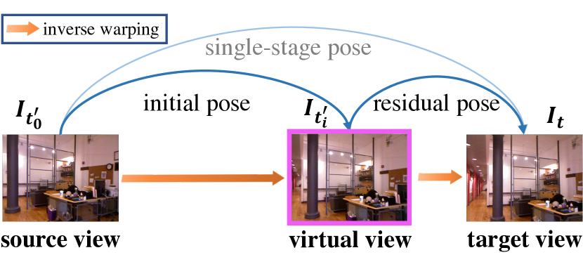
Figure 2: Residual Pose Estimation. A single-stage pose can be decomposed into an initial pose and a residual pose by virtual view synthesis.

Our residual pose module consists of a standard pose network and a residual pose network. In the first stage, the pose network takes a target image $I_{t}$ and a source image $I_{t^{\prime}_{0}}$ as input and predicts an initial camera pose ${T}_{t^{\prime}_{0}\rightarrow t}$, where the subscript $0$ in $t^{\prime}_{0}$ indicates that no transformation is applied over the source image yet. Then Equation (2) is used to bilinearly sample from the source image, reconstructing a warped target image $I_{t^{\prime}_{0}\rightarrow t}$ of a virtual view which is expected to be the same as the target image $I_{t}$ if the correspondences are solved accurately. However, it will not be the case due to inaccurate pose prediction. The transformation for this warping operation is defined as

$$I_{t^{\prime}_{0}\rightarrow t}=I_{t^{\prime}}\langle proj({D}_{t},{T}^{-1}_{t^{\prime}_{0}\rightarrow t},K)\rangle.$$ (12)

Next, we propose a residual pose network (see ResidualPoseNet in Figure 1) which takes the target image and the synthesized target image of a virtual view ($I_{t^{\prime}_{0}\rightarrow t}$) as input and outputs a residual camera pose ${T}^{res}_{(t^{\prime}_{0}\rightarrow t)\rightarrow t}$, representing the camera pose of the synthesized image $I_{t^{\prime}_{0}\rightarrow t}$ with respect to the target image $I_{t}$. Then, we bilinearly sample from the synthesized image as

$$I_{(t^{\prime}_{0}\rightarrow t)\rightarrow t}=I_{t^{\prime}_{0}\rightarrow t}\langle proj({D}_{t},{T}^{res\;-1}_{(t^{\prime}_{0}\rightarrow t)\rightarrow t},K)\rangle.$$ (13)

Once a new synthesized image of a virtual view is obtained, we can continue to estimate the residual camera poses for next view synthesis operation.

We define the general form of Equation (13) as

$$I_{t^{\prime}_{i}\rightarrow t}=I_{t^{\prime}_{i}}\langle proj({D}_{t},{T}^{res-1}_{t^{\prime}_{i}\rightarrow t},K)\rangle,i=0,1,\cdots\;.$$ (14)

by replacing the subscript $t^{\prime}_{0}\rightarrow t$ with $t^{\prime}_{1}$ to indicate that one warping transformation is applied, and similarly for the $i^{\rm th}$ transformation.

To this end, after multiple residual poses are estimated, the camera pose of source image $I_{t}^{\prime}$ with respect to the target image $I_{t}$ can be written as ${T}_{t\rightarrow t^{\prime}}={T}^{-1}_{t^{\prime}\rightarrow t}$ where

$${T}_{t^{\prime}\rightarrow t}=\prod_{i}{T}_{t^{\prime}_{i}\rightarrow t},i=\cdots,k,\cdots,1,0\;.$$ (15)

By iteratively estimating residual poses using a pose network and a residual pose network, we expect to obtain more accurate camera pose compared with the pose predicted from a single-stage pose network, so that a more accurate photometric reprojection loss can be built up for better depth prediction during the model training.

III-D Coordinates Convolutional Encoding

For self-supervised monocular depth estimation, most of existing methods are designed to induce relative camera poses given a pair of color images. In this work, we propose to incorporate coordinates information as a part of input channels along with the color information explicitly to provide additional coordinates cues for pose estimation.

We extend standard convolutional layers to coordinates convolutional layers by initializing extra channels to process coordinates information which is concatenated channel-wise to the input representations (see Coordinates Convolutional Encoding in Figure 1). Given a pair of 2D images, we encode two coordinates $x,y$ with color information $(r,g,b)$, resulting in the 8-channels input as $(r_{1},g_{1},b_{1},r_{2},g_{2},b_{2},i,j)$ where $(r_{1},g_{1},b_{1})$ and $(r_{2},g_{2},b_{2})$ are rgb values of color images, respectively. The $i$ coordinate channel is an $h\times w$ rank-1 matrix with its first row filled with 0’s, its second row with 1’s, its third with 2’s, etc. The $j$ coordinate channel is similar, but with columns filled in with constant values instead of rows. A linear scaling operation is applied over both $i$ and $j$ coordinate values to encode them in the range $[-1,1]$. We adopt coordinates convolutional layers [57] in the residual pose estimation module to process 8-channels input for iterative pose estimation, and the pose estimation can be written as follows:

$$T_{t\rightarrow t^{\prime}}=RPModule(\mathbf{\Omega};Concat(I_{t},I_{t^{\prime}},i,j))$$ (16)

where $RPModule$ is the proposed pose estimation module, $\Omega$ is the parameters of the module which are to be optimized.

IV Experiments

IV-A Implementation Details

We implement our model using PyTorch [60]. In the depth factorization module, we use the same depth network as in Monodepth2 [5]; for the transformer-based scale regression network, we use a transformer module followed by two basic residual blocks and then three fully-connected layers with a dropout layer in-between. The dropout rate is empirically set to 0.5. In the residual pose module, we let the residual pose networks use a common architecture as in Monodepth2 [5] which consists of a shared pose encoder and an independent pose regressor. In the coordinates encoding module, 2D coordinates information $(i,j)$ are directly concatenated with $(r,g,b)$ channels of color images as the input and the convolutional layers are initialized with ImageNet-pretrained weights. Each experiment is trained for 40 epochs using the Adam [61] optimizer and the learning rate is set to $10^{-4}$ for the first 20 epochs and it drops to $10^{-5}$ for remaining epochs. The smoothness term $\tau$ is set as 0.001. The consistency term $\gamma$ are set as 0.1 for EuRoC MAV dataset, 0.035 for NYUv2, ScanNet and 7-Scenes datasets, respectively.

TABLE I: Comparison of our method to existing supervised and self-supervised methods on NYUv2 [14]. Best results among supervised and self-supervised methods are in bold.

Methods	Supervision	Error Metric		Accuracy Metric
		AbsRel	RMS	$\delta_{1}$	$\delta_{2}$	$\delta_{3}$
Make3D [21]	✓	0.349	1.214	0.447	0.745	0.897
Depth Transfer [62]	✓	0.349	1.210	-	-	-
Liu et al.  [63]	✓	0.335	1.060	-	-	-
Ladicky et al.  [64]	✓	-	-	0.542	0.829	0.941
Li et al.  [65]	✓	0.232	0.821	0.621	0.886	0.968
Roy et al.  [66]	✓	0.187	0.744	-	-
Liu et al.  [67]	✓	0.213	0.759	0.650	0.906	0.976
Wang et al.  [68]	✓	0.220	0.745	0.605	0.890	0.970
Eigen et al.  [1]	✓	0.158	0.641	0.769	0.950	0.988
Chakrabarti et al.  [69]	✓	0.149	0.620	0.806	0.958	0.987
Laina et al.  [24]	✓	0.127	0.573	0.811	0.953	0.988
Li et al.  [26]	✓	0.143	0.635	0.788	0.958	0.991
DORN [2]	✓	0.115	0.509	0.828	0.965	0.992
Ranftl et al.  [36]	✓	0.110	0.357	0.904	0.988	0.994
VNL [11]	✓	0.108	0.416	0.875	0.976	0.994
Bhat et al.  [25]	✓	0.103	0.364	0.903	0.984	0.997
Fang et al.  [70]	✓	0.101	0.412	0.868	0.958	0.986
Zhou et al.  [8]	✗	0.208	0.712	0.674	0.900	0.968
Zhao et al.  [9]	✗	0.189	0.686	0.701	0.912	0.978
Monodepth2 [5]	✗	0.160	0.601	0.767	0.949	0.988
SC-Depth [38]	✗	0.159	0.608	0.772	0.939	0.982
P2Net (3-frame) [71]	✗	0.159	0.599	0.772	0.942	0.984
P2Net (5-frame) [71]	✗	0.147	0.553	0.801	0.951	0.987
Bian et al.  [45]	✗	0.147	0.536	0.804	0.950	0.986
Bian et al.  [10]	✗	0.138	0.532	0.820	0.956	0.989
MonoIndoor (Ours)	✗	0.132	0.517	0.834	0.961	0.990

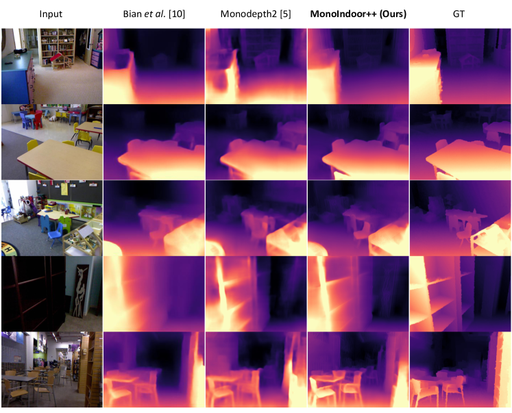
Figure 3: Qualitative comparison on NYUv2 [14]. Images form the left to the right are: input, depth from  [10], [5], MonoIndoor++(Ours), ground-truth depth. Compared with both the baseline method Monodepth2 [5] and recent work [10], our model produces accurate depth maps that are closer to the ground-truth.

IV-B Datasets

IV-B1 NYUv2 [14]

The NYUv2 depth dataset contains 464 indoor video sequences which are captured by a hand-held Microsoft Kinect RGB-D camera. The dataset is widely used as a challenging benchmark for depth prediction. The resolution of videos is 640$\times$ 480. Images are rectified with provided camera intrinsics to remove image distortion. We use the official training and validation splits which include 302 and 33 sequences, respectively. We use officially provided 654 images with dense labelled depth maps for testing. During training, images are resized to 320$\times$256.

IV-B2 EuRoC MAV [15]

The EuRoC MAV Dataset contains 11 video sequences captured in two main scenes, a machine hall and a vicon room. Sequences are categorized as easy, medium and difficult according to the varying illumination and camera motions. For the training, we use three sequences of “Machine hall” (MH_01, MH_02, MH_04) and two sequences of “Vicon room” (V1_01 and V1_02). Images are rectified with provided camera intrinsics to remove image distortion. During training, images are resized to 512$\times$256. We use the Vicon room sequence V1_03, V2_01, V2_02 and V2_03 for testing where the ground-truth depths are generated by projecting Vicon 3D scans onto the image planes. During training, images are resized to 512$\times$256. In addition, we use V2_01 for ablation studies (see Section IV-E1 and Section IV-E2).

IV-B3 ScanNet [19]

The ScanNet dataset contains RGB-D videos of 1513 indoor scans, which is captured by handheld devices. The dataset is annotated with 3D camera poses and instance-level semantic segmentations and is widely used on several 3D scene understanding tasks, including 3D object classification, semantic voxel labeling, and CAD model retrieval. We use officially released train-validation-test splits. The resolution of color images is $1296\times 968$. During training, images are resized to 320$\times$256.

IV-B4 7-Scenes [20]

7-Scenes dataset contains a number of video sequences captured in 7 different indoor scenes, i.e., office, stairs, etc. Each scene contains 500-1000 frames. All scenes are recorded using a handheld Kinect RGB-D camera at the resolution of $640\times 480$. We use the official train-test split. During training, images are resized to 320$\times$256.

IV-C Evaluation Metrics

We use both error metrics and accuracy metrics proposed in [23] for evaluation on all datasets, which include the mean absolute relative error (AbsRel), root mean squared error (RMS) and the accuracy under threshold ($\delta_{i}<1.25^{i},i=1,2,3$). Following previous self-supervised depth estimation methods [5, 9, 10], we multiply the predicted depth maps by a scalar that matches the median with that of the ground-truth because self-supervised monocular methods cannot recover the metric scale. The predicted depths are capped at 10m in all indoor datasets except the EuRoC MAV dataset which one is set as 20m because it contains “Machine hall” scenes with observed large depth scale.

IV-D Experimental Results

IV-D1 Results on NYUv2 Depth Dataset

In this section, we evaluate our MonoIndoor++ on the NYUv2 depth dataset [14]. Following [9, 45], the raw dataset is firstly downsampled 10 times along the temporal dimension to remove redundant frames, resulting in $\sim 20K$ images for training.

Quantitative Results Table I presents the quantitative results of our model MonoIndoor++ and both state-of-the-art (SOTA) supervised and self-supervised methods on NYUv2. It shows that our model outperforms previous self-supervised SOTA methods [5, 71, 10], reaching the best results across all metrics. Specifically, compared with Monodepth2 [5], which is our baseline method, our method improves monocular depth prediction performance significantly, reducing AbsRel from 16.0% to 13.2% and increasing $\delta_{1}$ from 76.7% to 83.4%. Besides, compared to a recent self-supervised method by Bian et al.  [45, 10] which removes rotations via “weak rectification” with a data preprocessing step, our method gives the better performance without additional data preprocessing. It is noted that NYUv2 is very challenging and many previous self-supervised methods [40] fail to get satisfactory results. In addition to that, our model outperforms a group of supervised methods [63, 64, 1, 69, 26] and closes the performance gap between the self-supervised methods and fully-supervised methods [24, 2].

TABLE II: Quantitative results and comparisons between our MonoIndoor++ by integrating our proposed core modules with the baseline Monodepth2 [5] on the test sequence V1_03, V2_01 V2_02, V2_03 of EuRoC. Best results are in bold.

Method	Residual Pose	Depth Factorization	Coordinates Encoding	Error Metric		Accuracy Metric			Error Metric		Accuracy Metric
				AbsRel	RMSE	$\delta_{1}$	$\delta_{2}$	$\delta_{3}$	AbsRel	RMSE	$\delta_{1}$	$\delta_{2}$	$\delta_{3}$
				V1_03					V2_01
Monodepth2 [5]	✗	✗	✗	0.110	0.413	0.889	0.983	0.996	0.157	0.567	0.786	0.941	0.986
MonoIndoor++ (Ours)	✓	✗	✗	0.100	0.379	0.913	0.987	0.997	0.141	0.518	0.815	0.961	0.991
MonoIndoor++ (Ours)	✓	✓	✗	0.080	0.309	0.944	0.990	0.998	0.125	0.466	0.840	0.965	0.993
MonoIndoor++ (Ours)	✓	✓	✓	0.079	0.303	0.949	0.991	0.998	0.115	0.439	0.861	0.972	0.992
				V2_02					V2_03
Monodepth2 [5]	✗	✗	✗	0.156	0.645	0.776	0.945	0.985	0.171	0.620	0.734	0.944	0.988
MonoIndoor++ (Ours)	✓	✗	✗	0.141	0.583	0.814	0.958	0.989	0.147	0.538	0.806	0.963	0.989
MonoIndoor++ (Ours)	✓	✓	✗	0.142	0.581	0.802	0.952	0.990	0.140	0.502	0.810	0.964	0.993
MonoIndoor++ (Ours)	✓	✓	✓	0.133	0.551	0.830	0.964	0.991	0.134	0.482	0.829	0.967	0.993

Qualitative Results Figure 3 visualizes the predicted depth maps on NYUv2. Compared with the results from the baseline method Monodepth2 [5] and recent work [10], depth maps predicted from our model (MonoIndoor++) are more precise and closer to the ground-truth. For instance, looking at the fourth column in the first row, the depth in the region of cabinet predicted from our model is much sharper and cleaner, being close to the ground-truth (the last column). These qualitative results are consistent with our quantitative results in Table I.

IV-D2 Results on EuRoC MAV Dataset

In this section, we present evaluation of self-supervised monocular depth prediction and pose estimation. As there are not many public results on the EuRoC MAV dataset [15], we mainly compare between our MonoIndoor++ and the baseline method Monodepth2 [5].

Quantitative Results We present and validate the effectiveness of each module of our MonoIndoor++ and experimental results are shown Table II. It is observed that the depth prediction performance can be improved by adding each of our proposed modules. Our full model achieves the best performance across all evaluation metrics on various scenes including “difficult” scenes “Vicon room 103” and “Vicon room 203”. For instance, on “Vicon room 201” (V2_01), adding our residual pose module reduces the AbsRel from 15.7% to 14.1% and increases the $\delta_{1}$ from 78.6% to 81.5%, adding our depth factorization module reduces the AbsRel to 12.4% and improves the $\delta_{1}$ to 84.0% and adding our coordinates convolutional encoding reduces the AbsRel to 11.5% and increases the $\delta_{1}$ to 86.1% further. Similar improvements can be observed on other test sequences.

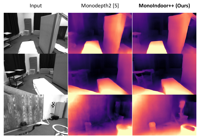
Figure 4: Qualitative comparison of depth prediction on EuRoC MAV. Our MonoIndoor++ produces more accurate and cleaner depth maps.

Qualitative Results We present the qualitative results and comparisons of depth maps predicted by the baseline method Monodepth2 [5] and our MonoIndoor++ in Figure 4. There are no ground-truth dense depth maps on the EuRoC MAV dataset. From Figure 4, it is clear that the depth maps generated by our model are much better than the ones by Monodepth2. For instance, in the third row, our model can predict precise depths for the hole region at the right-bottom corner whereas such a hole structure in the depth map by Monodepth2 is missing. These observations are also consistent with the better quantitative results in Table II, proving the superiority of our model.

TABLE III: Relative pose evalution on the EuRoC MAV [15] dataset. Results show the average absolute trajectory error(ATE), and the relative pose error(RPE) in meters and degrees, respectively. Scene: test sequence name.

Scene	Methods	ATE(m)	RPE(m)	RPE(°)
V1_03	Monodepth2 [5]	0.0681	0.0686	1.3237
	MonoIndoor++ (Ours)	0.0557	0.0542	0.5599
V2_01	Monodepth2 [5]	0.0266	0.0199	1.1985
	MonoIndoor++ (Ours)	0.0229	0.0050	1.1239
V2_02	Monodepth2 [5]	0.0624	0.0481	6.4135
	MonoIndoor++ (Ours)	0.0517	0.0350	7.1928
V2_03	Monodepth2 [5]	0.0670	0.0355	5.3532
	MonoIndoor++ (Ours)	0.0644	0.0676	4.8559

TABLE IV: Comparison of our method to latest self-supervised methods on RGB-D 7-Scenes [20]. Best results are in bold

. Scenes Bian et al.  [45] Monodepth2[5] (Baseline) MonoIndoor++ (Ours) Before Fine-tuning After Fine-tuning Before Fine-tuning After Fine-tuning Before Fine-tuning After Fine-tuning AbsRel Acc $\delta_{1}$ AbsRel Acc $\delta_{1}$ AbsRel Acc $\delta_{1}$ AbsRel Acc $\delta_{1}$ AbsRel Acc $\delta_{1}$ AbsRel Acc $\delta_{1}$ Chess 0.169 0.719 0.103 0.880 0.193 0.654 0.123 0.853 0.157 0.750 0.097 0.888 Fire 0.158 0.758 0.089 0.916 0.190 0.670 0.091 0.927 0.150 0.768 0.077 0.939 Heads 0.162 0.749 0.124 0.862 0.206 0.661 0.130 0.855 0.171 0.727 0.106 0.889 Office 0.132 0.833 0.096 0.912 0.168 0.748 0.105 0.897 0.130 0.837 0.083 0.934 Pumpkin 0.117 0.857 0.083 0.946 0.135 0.816 0.116 0.877 0.102 0.895 0.078 0.945 RedKitchen 0.151 0.78 0.101 0.896 0.168 0.733 0.108 0.884 0.144 0.795 0.094 0.915 Stairs 0.162 0.765 0.106 0.855 0.146 0.806 0.127 0.825 0.155 0.753 0.104 0.857

Pose Evaluation In Table III, we evaluate the proposed residual pose estimation module on all test sequences V1_03, V2_01, V2_02 and V2_03 of the EuRoC MAV [15]. We follow [72] to evaluate relative camera poses estimated by our residual pose estimation module. We use the following evaluation metrics: absolute trajectory error (ATE) which measures the root-mean square error between predicted camera poses and ground-truth, and relative pose error (RPE) which measures frame-to-frame relative pose error in meters and degrees, respectively. As shown in Table III, compared with the baseline model Monodepth2 [5] which employs one-stage pose network, using our method leads to improved relative pose estimation across evaluation metrics on most test scenes. Specifically, on the scene V1_03, the ATE by our MonoIndoor is significantly decreased from 0.0681 meters to 0.0557 meters and RPE(°) is reduced from 1.3237° to 0.5599°. Similar observations are made on the scene V2_02, where the ATE by our MonoIndoor++ is significantly decreased from 0.0681 meters to 0.0557 meters.

IV-D3 Results on RGB-D 7-Scenes Dataset

In this section, we evaluate our MonoIndoor++ on the RGB-D 7-Scenes dataset [20]. Following [45], we extract one image from every 30 frames in each video sequence. For training, we first pre-train our model on the NYUv2 dataset, and then fine-tune the pre-trained model on each scene of 7-Scenes dataset.

Table IV presents the quantitative results and comparisons of our model MonoIndoor++ and latest state-of-the-art (SOTA) self-supervised methods on 7-Scenes dataset. It can be observed that our model outperforms the baseline method Monodepth2 [5] significantly on each scene. Further, compared to the model [45], our method achieve the best performance on most scenes before and after fine-tuning using NYUv2 pretrained models, which demonstrates better generalizability and capability of our model. Moreover, the results show that our method can perform well in a variety of different scenes.

IV-D4 Results on ScanNet Dataset

In this section, we evaluate our MonoIndoor++ on the ScanNet dataset [19]. Referring to [73], the raw dataset is firstly downsampled 10 times along the temporal dimension and then $\sim 100K$ images are randomly selected for training. During testing, $\sim 4K$ are sampled from 100 different testing scenes to evaluate the trained model.

Self-supervised Depth Estimation Evaluation Table V presents the quantitative results of our model MonoIndoor++ and both state-of-the-art (SOTA) supervised and self-supervised methods on ScanNet. It shows that our model outperforms the previous self-supervised method [74] in depth prediction, reaching the best results across all metrics. In addition to that, our model outperforms a group of supervised methods [75, 73].

TABLE V: Comparison of our method to existing supervised and self-supervised methods on ScanNet [19]. Best results among supervised and self-supervised methods are in bold.

Methods	Supervision	AbsRel	SqRel	RMS	RMSlog
Photometric BA [76]	✓	0.268	0.427	0.788	0.330
DeMoN [75]	✓	0.231	0.520	0.761	0.289
BANet [73]	✓	0.161	0.092	0.346	0.214
DeepV2D [31]	✓	0.069	0.018	0.196	0.099
NeuralRecon [77]	✓	0.047	0.024	0.164	0.093
Gu et al.  [74]	✗	0.140	0.127	0.496	0.212
MonoIndoor++ (Ours)	✗	0.113	0.048	0.302	0.148

Zero-shot Generalization We present the zero-shot generalization results of self-supervised depth prediction on ScanNet [19] in Table VI, where we evaluate the proposed MonoIndoor++ pretrained on NYUv2 dataset. From Table VI, it is observed that our NYUv2 pretrained model generalizes better than other recent methods to new dataset. Besides, we show the zero-shot generalization results of relative pose estimation on ScanNet in Table VII. We follow [71, 31] to use 2000 image pairs selected from diverse indoor scenes for pose evaluation. It can be observed that our method outperforms other self-supervised methods. Specifically, compared to Bian et al.  [10], our method significantly reduces tr (cm) from 0.55 meters to 0.27 meters and decreases rot (deg) from 1.82 to 1.19. Both depth and pose results validate the good zero-shot generalizability and capability of our method.

TABLE VI: Zero-shot generalization of our method for self-supervised depth estimation on ScanNet [19]. Best results are in bold.

Methods	Supervision	Error Metric		Accuracy Metric
		AbsRel	RMS	$\delta_{1}$	$\delta_{2}$	$\delta_{3}$
Latina et al.  [24]	✓	0.141	0.339	0.811	.958	0.990
VNL [11]	✓	0.123	0.306	0.848	0.964	0.991
Zhao et al.  [9]	✗	0.179	0.415	0.726	0.927	0.980
Bian et al.  [38]	✗	0.169	0.392	0.749	0.938	0.983
Bian et al.  [10]	✗	0.156	0.361	0.781	0.947	0.987
Monodepth2 [5]	✗	0.170	0.401	0.730	0.948	0.991
MonoIndoor++ (Ours)	✗	0.138	0.347	0.810	0.967	0.993

TABLE VII: Zero-shot generalization of our method for relative pose estimation on ScanNet [19]. Best results are in bold.

Methods	rot (deg)	tr (deg)	tr (cm)
Zhou et al.  [8]	1.96	39.17	1.4
Monodepth2 [5]	2.03	41.12	0.83
P2Net [71]	1.86	35.11	0.89
Bian et al.  [10]	1.82	39.41	0.55
MonoIndoor++ (Ours)	1.19	21.33	0.27

IV-E Ablation Studies

IV-E1 Effects of each proposed module

TABLE VIII: Ablation results of our MonoIndoor++ and comparison with the baseline method on the test sequence V2_01 of EuRoC and NYUv2 datasets. Best results are in bold.

Method	Residual Pose	Depth Factorization	Coordinates Encoding	Depth Consistency	EuRoC MAV V2_01					NYUv2
					Error Metric		Accuracy Metric			Error Metric		Accuracy Metric
					AbsRel	RMSE	$\delta_{1}$	$\delta_{2}$	$\delta_{3}$	AbsRel	RMSE	$\delta_{1}$	$\delta_{2}$	$\delta_{3}$
Monodepth2 [5]	✗	✗	✗	✗	0.157	0.567	0.786	0.941	0.986	0.16	0.601	0.767	0.949	0.988
MonoIndoor++ (Ours)	✓	✗	✗	✗	0.141	0.518	0.815	0.961	0.991	0.142	0.553	0.813	0.958	0.988
MonoIndoor++ (Ours)	✓	✗	✓	✗	0.129	0.481	0.843	0.971	0.990	0.139	0.545	0.821	0.958	0.989
MonoIndoor++ (Ours)	✗	✓	✗	✗	0.149	0.535	0.805	0.955	0.987	0.152	0.576	0.792	0.951	0.987
MonoIndoor++ (Ours)	✓	✓	✗	✗	0.133	0.501	0.833	0.961	0.987	0.139	0.549	0.818	0.958	0.988
MonoIndoor++ (Ours)	✓	✓	✗	✓	0.125	0.466	0.840	0.965	0.993	0.134	0.526	0.823	0.958	0.989
MonoIndoor++ (Ours)	✓	✓	✓	✓	0.115	0.439	0.861	0.972	0.992	0.132	0.517	0.834	0.961	0.990

Figure 5: Qualitative ablation comparisons of depth prediction on NYUv2. Our full model with both depth factorization and residual pose modules produce better depth maps.

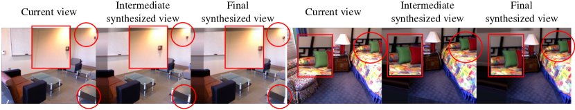
Figure 6: Intermediate synthesized views on NYUv2.

In this section, we perform ablation studies for each module in our proposed MonoIndoor++ on the NYUv2 dataset [14] and the test scene “V2_01” of the EuRoC MAV dataset [15] in Table VIII.

Specifically, We first perform ablation study for the residual pose estimation module. In Table VIII (see row 2 and 3), improved performance can be observed by using the residual pose module, decreasing the AbsRel from 15.7% to 14.1% and increasing $\delta_{1}$ to 81.5% on EuRoC MAV V2_01, and decreasing the AbsRel from 16% to 14.2% and increasing $\delta_{1}$ to 81.3% on NYUv2.

Next, we experiment to validate the effectiveness of the depth factorization module (see row 2 and 5). Comparing with Monodepth2 which predicts depth without any guidance of global scales, by using the depth factorization module with a separate scale network, we observe an improved performance from 15.7% down to 14.9% for AbsRel and from 78.6% up to 80.5% for $\delta_{1}$ on EuRoC MAV V2_01, and decreasing the AbsRel to 15.2% and increasing $\delta_{1}$ to 79.2% on NYUv2.

In addition, by applying the residual pose estimation module along with either the depth factorization module (row 6) or coordinates convolutional encoding (row 4), the performance can be improved consistently. Further, we present ablation results by using depth consistency loss with the residual pose estimation module and the depth factorization module (see row 6 and 7). Also, ablation results of our full model with and without coordinate convolutional encoding are shown in row 7 and row 8.

Last but not the least, using our full model MonoIndoor++, significant improvements can be achieved across all evaluation metrics. For instance, the AbsRel is reduced to 11.5% and the $\delta_{1}$ is increased to 86.1% on EuRoC MAV V2_01 and the AbsRel is reduced to 13.2% and $\delta_{1}$ is increased to 83.2% on NYUv2. These ablation results clearly prove the effectiveness of the proposed modules.

We also present the exemplar depth visualizations by our proposed modules on NYUv2 dataset in Figure 5. In addition, we visualize intermediate and final synthesized views compared with the current view on NYUv2 in Figure 6. Highlighted regions show that final synthesized views are better than the intermediate synthesized views and closer to the current view.

IV-E2 Effects of network design for transformer-based scale regression network

We perform ablation studies for our network design choices for the transformer-based scale regression network in depth factorization module on the test sequence V2_01 of the EuRoC MAV dataset [14]. Firstly, we consider the following designs as the backbone of our scale regression network: I) a pre-trained ResNet-18 [78] followed by a group of Convolutional-BN-ReLU layers; II) a pre-trained ResNet-18 [78] followed by two residual blocks; III) a lightweight network with two residual blocks which shares the feature maps from the depth encoder as input. These three choices are referred to as the ScaleCNN, ScaleNet and ScaleRegressor, respectively in Table IX. Next, we validate the effectiveness of adding new components into our backbone design. As described in Section III-B, we mainly integrate two sub-modules: i) a transformer module and ii) a probabilistic scale regression block.

TABLE IX: Ablation results of design choices and the effectiveness of components in the transformer-based scale regression network of our model (MonoIndoor++) on EuRoC MAV [15]. Porb. Reg.: the probabilistic scale regression block. Note: we only use the residual pose estimation module when experimenting with different network designs for the depth factorization module.

Network Design	Attention	Prob. Reg.	Error Metric		Accuracy Metric
			AbsRel	RMSE	$\delta_{1}$	$\delta_{2}$	$\delta_{3}$
I. ScaleCNN	✓	✓	0.140	0.518	0.821	0.956	0.985
II. ScaleNet	✓	✓	0.141	0.519	0.817	0.959	0.988
III. ScaleRegressor	✗	✗	0.139	0.508	0.817	0.960	0.987
III. ScaleRegressor	✓	✗	0.135	0.501	0.825	0.964	0.989
III. ScaleRegressor	✓	✓	0.125	0.466	0.840	0.965	0.993

As shown in Table IX, the best performance is achieved by ScaleRegressor that uses transformer module and probabilistic scale regression. It proves that sharing features with the depth encoder is beneficial to scale estimation. Comparing the results of three ScaleRegressor variants, the performance gradually improves as we add more components (i.e.., attention and probabilistic scale regression (Prob. Reg.)). Specifically, adding the transformer module improves the overall performance over the baseline backbone; adding the probabilistic regression block leads to a further improvement, which validates the effectiveness of our proposed sub-modules.

IV-E3 Ablation results of coordinates convolutional encoding

We present ablation studies for the encoding position of the coordinates convolutional encoding module on the NYUv2 dataset [14] in Tabel X. To explore the effectiveness of using coordinates encoding technique, we only run our MonoIndoor++ with the residual pose estimation module. We perform coordinates convolutional encoding with the following choices. Specifically, we first encode coordinates information with the color image pairs and extend coordinates convolutional layers to process combined input data. Second, we perform coordinates encoding operations with the feature representations outputted from the pose encoder and the processed features are taken as the input to the pose decoder. Third, we incorporate coordinates encoding operations with both input and features from pose encoder for pose estimation.

TABLE X: Ablation results of encoding position for coordinates conovlutional with our MonoIndoor++ on NYUv2. Init.: initialization of weights.

Model	Encoding Position	Error Metric		Accuracy Metric
		AbsRel	RMS	$\delta_{1}$	$\delta_{2}$	$\delta_{3}$
MonoIndoor	✗	0.142	0.553	0.813	0.958	0.988
MonoIndoor++ (Random Init.)	Input	0.140	0.543	0.817	0.959	0.989
MonoIndoor++ (ImageNet Init.)	Input	0.139	0.545	0.821	0.958	0.989
MonoIndoor++ (ImageNet Init.)	Encoder Features	0.145	0.565	0.806	0.954	0.988
MonoIndoor++ (ImageNet Init.)	Input & Encoder Features	0.141	0.554	0.815	0.957	0.989

From the Table X, it can be observed that, by using coordinates convolutional encoding in residual pose estimation module, performance can be improved. For instance, the AbsRel is decreased to 13.9% from 14.2% and the $\delta_{1}$ is improved from 81.7% to 82.1%. Besides, comparing with encoding coordinates information with feature representations after the pose encoder, applying the coordinates convolutional encoding operation over the input image pairs directly gives the best performance. Further, we test two different initialization methods for coordinates convolutional layers which are with random initializations or ImageNet-pretrained [79] initialization, respectively. The coordinates convolutional encoding layers which are initialized with ImageNet-pretrained weights give slightly improved performance compared to ones with random weights.

V Conclusions

In this work, a novel monocular self-supervised depth estimation framework, called the MonoIndoor++, has been proposed to predict depth map of a single image in indoor environments. The proposed model consists of three modules: (a) a novel depth factorization module with a transformer-based scale regression network which is designed to jointly learn a global depth scale factor and a relative depth map from an input image, (b) a novel residual pose estimation module which is proposed to estimate accurate relative camera poses for novel view synthesis of self-supervised training that decomposes a global pose into an initial pose and one or a few residual poses, which in turn improves the performance of the depth model, (c) a coordinates convolutional encoding module which is utilized to encode coordinates information explicitly to provide additional cues for the residual pose estimation module. Comprehensive evaluation results and ablation studies have been conducted on a wide-variety of indoor datasets, establishing the state-of-the-art performance and demonstrating the effectiveness and universality of our proposed methods.

References

- [1] D. Eigen and R. Fergus, “Predicting depth, surface normals and semantic labels with a common multi-scale convolutional architecture,” in ICCV, 2015.
- [2] H. Fu, M. Gong, C. Wang, K. Batmanghelich, and D. Tao, “Deep ordinal regression network for monocular depth estimation,” in CVPR, 2018.
- [3] R. Garg, V. K. Bg, G. Carneiro, and I. Reid, “Unsupervised cnn for single view depth estimation: Geometry to the rescue,” in ECCV, 2016.
- [4] T. Zhou, M. Brown, N. Snavely, and D. G. Lowe, “Unsupervised learning of depth and ego-motion from video,” in CVPR, 2017.
- [5] C. Godard, O. Mac Aodha, M. Firman, and G. J. Brostow, “Digging into self-supervised monocular depth estimation,” in ICCV, 2019.
- [6] X. Guo, H. Li, S. Yi, J. Ren, and X. Wang, “Learning monocular depth by distilling cross-domain stereo networks,” in ECCV, 2018.
- [7] A. Geiger, P. Lenz, and R. Urtasun, “Are we ready for autonomous driving? the kitti vision benchmark suite,” in CVPR, 2012.
- [8] J. Zhou, Y. Wang, K. Qin, and W. Zeng, “Moving indoor: Unsupervised video depth learning in challenging environments,” in ICCV, 2019, pp. 8618–8627.
- [9] W. Zhao, S. Liu, Y. Shu, and Y.-J. Liu, “Towards better generalization: Joint depth-pose learning without posenet,” in CVPR, 2020.
- [10] J. Bian, H. Zhan, N. Wang, T.-J. Chin, C. Shen, and I. Reid, “Auto-rectify network for unsupervised indoor depth estimation,” TPAMI, 2021.
- [11] W. Yin, Y. Liu, C. Shen, and Y. Yan, “Enforcing geometric constraints of virtual normal for depth prediction,” in ICCV, 2019.
- [12] Y. Zou, P. Ji, , Q.-H. Tran, J.-B. Huang, and M. Chandraker, “Learning monocular visual odometry via self-supervised long-term modeling,” in ECCV, 2020.
- [13] R. Mur-Artal and J. D. Tardós, “Orb-slam2: An open-source slam system for monocular, stereo, and rgb-d cameras,” TOR, vol. 33, no. 5, pp. 1255–1262, 2017.
- [14] N. Silberman, D. Hoiem, P. Kohli, and R. Fergus, “Indoor segmentation and support inference from rgb-d images,” in ECCV, 2012.
- [15] J. L. Schonberger and J.-M. Frahm, “Structure-from-motion revisited,” in CVPR, 2016.
- [16] A. Dosovitskiy, L. Beyer, A. Kolesnikov, D. Weissenborn, X. Zhai, T. Unterthiner, M. Dehghani, M. Minderer, G. Heigold, S. Gelly, J. Uszkoreit, and N. Houlsby, “An image is worth 16x16 words: Transformers for image recognition at scale,” in ICLR, 2021.
- [17] P. Ji, R. Li, B. Bhanu, and Y. Xu, “Monoindoor: Towards good practice of self-supervised monocular depth estimation for indoor environments,” in ICCV, 2021.
- [18] M. Burri, J. Nikolic, P. Gohl, T. Schneider, J. Rehder, S. Omari, M. W. Achtelik, and R. Siegwart, “The euroc micro aerial vehicle datasets,” IJRR, vol. 35, no. 10, pp. 1157–1163, 2016.
- [19] A. Dai, A. X. Chang, M. Savva, M. Halber, T. Funkhouser, and M. Nießner, “Scannet: Richly-annotated 3d reconstructions of indoor scenes,” in CVPR, 2017.
- [20] J. Shotton, B. Glocker, C. Zach, S. Izadi, A. Criminisi, and A. Fitzgibbon, “Scene coordinate regression forests for camera relocalization in rgb-d images,” in CVPR, 2013.
- [21] A. Saxena, M. Sun, and A. Y. Ng, “Make3d: Learning 3d scene structure from a single still image,” TPAMI, vol. 31, no. 5, pp. 824–840, 2008.
- [22] J. L. Schönberger, E. Zheng, M. Pollefeys, and J.-M. Frahm, “Pixelwise view selection for unstructured multi-view stereo,” in ECCV, 2016.
- [23] D. Eigen, C. Puhrsch, and R. Fergus, “Depth map prediction from a single image using a multi-scale deep network,” arXiv preprint arXiv:1406.2283, 2014.
- [24] I. Laina, C. Rupprecht, V. Belagiannis, F. Tombari, and N. Navab, “Deeper depth prediction with fully convolutional residual networks,” in 3DV, 2016.
- [25] S. F. Bhat, I. Alhashim, and P. Wonka, “Adabins: Depth estimation using adaptive bins,” in CVPR, 2021.
- [26] J. Li, R. Klein, and A. Yao, “A two-streamed network for estimating fine-scaled depth maps from single rgb images,” in ICCV, 2017.
- [27] M. Song, S. Lim, and W. Kim, “Monocular depth estimation using laplacian pyramid-based depth residuals,” T-CSVT, vol. 31, no. 11, pp. 4381–4393, 2021.
- [28] Y. Cao, T. Zhao, K. Xian, C. Shen, Z. Cao, and S. Xu, “Monocular depth estimation with augmented ordinal depth relationships,” T-CSVT, vol. 30, no. 8, pp. 2674–2682, 2020.
- [29] Y. Cao, Z. Wu, and C. Shen, “Estimating depth from monocular images as classification using deep fully convolutional residual networks,” T-CSVT, vol. 28, no. 11, pp. 3174–3182, 2018.
- [30] B. Ummenhofer, H. Zhou, J. Uhrig, N. Mayer, E. Ilg, A. Dosovitskiy, and T. Brox, “Demon: Depth and motion network for learning monocular stereo,” in CVPR, 2017, pp. 5038–5047.
- [31] Z. Teed and J. Deng, “Deepv2d: Video to depth with differentiable structure from motion,” in ICLR, 2018.
- [32] Z. Li and N. Snavely, “Megadepth: Learning single-view depth prediction from internet photos,” in CVPR, 2018.
- [33] Z. Li, T. Dekel, F. Cole, R. Tucker, N. Snavely, C. Liu, and W. T. Freeman, “Learning the depths of moving people by watching frozen people,” in CVPR, 2019.
- [34] Z. Teed and J. Deng, “DROID-SLAM: Deep Visual SLAM for Monocular, Stereo, and RGB-D Cameras,” in NeurIPS, 2021.
- [35] R. Ranftl, K. Lasinger, D. Hafner, K. Schindler, and V. Koltun, “Towards robust monocular depth estimation: Mixing datasets for zero-shot cross-dataset transfer,” PAMI, vol. 44, no. 3, pp. 1623–1637, 2022.
- [36] R. Ranftl, A. Bochkovskiy, and V. Koltun, “Vision transformers for dense prediction,” in ICCV, 2021.
- [37] C. Godard, O. Mac Aodha, and G. J. Brostow, “Unsupervised monocular depth estimation with left-right consistency,” in CVPR, 2017.
- [38] J.-W. Bian, Z. Li, N. Wang, H. Zhan, C. Shen, M.-M. Cheng, and I. Reid, “Unsupervised scale-consistent depth and ego-motion learning from monocular video,” in NeurIPS, 2019.
- [39] C. Wang, J. M. Buenaposada, R. Zhu, and S. Lucey, “Learning depth from monocular videos using direct methods,” in CVPR, 2018.
- [40] Z. Yin and J. Shi, “Geonet: Unsupervised learning of dense depth, optical flow and camera pose,” in CVPR, 2018.
- [41] Y. Zou, Z. Luo, and J.-B. Huang, “DF-Net: Unsupervised joint learning of depth and flow using cross-task consistency,” in ECCV, 2018.
- [42] R. Wang, S. M. Pizer, and J.-M. Frahm, “Recurrent neural network for (un-) supervised learning of monocular video visual odometry and depth,” in CVPR, 2019.
- [43] L. Tiwari, P. Ji, Q.-H. Tran, B. Zhuang, S. Anand, and M. Chandraker, “Pseudo rgb-d for self-improving monocular slam and depth prediction,” in ECCV, 2020.
- [44] J. Watson, O. M. Aodha, V. Prisacariu, G. Brostow, and M. Firman, “The Temporal Opportunist: Self-Supervised Multi-Frame Monocular Depth,” in CVPR, 2021.
- [45] J.-W. Bian, H. Zhan, N. Wang, T.-J. Chin, C. Shen, and I. Reid, “Unsupervised depth learning in challenging indoor video: Weak rectification to rescue,” arXiv preprint arXiv:2006.02708, 2020.
- [46] X. Wang, R. Girshick, A. Gupta, and K. He, “Non-local neural networks,” in CVPR, 2018.
- [47] A. Vaswani, N. Shazeer, N. Parmar, J. Uszkoreit, L. Jones, A. N. Gomez, L. u. Kaiser, and I. Polosukhin, “Attention is all you need,” in NeurIPS, 2017.
- [48] Z. Liu, Y. Lin, Y. Cao, H. Hu, Y. Wei, Z. Zhang, S. Lin, and B. Guo, “Swin transformer: Hierarchical vision transformer using shifted windows,” in ICCV, 2021.
- [49] Z. Liu, H. Hu, Y. Lin, Z. Yao, Z. Xie, Y. Wei, J. Ning, Y. Cao, Z. Zhang, L. Dong, F. Wei, and B. Guo, “Swin transformer v2: Scaling up capacity and resolution,” in CVPR, 2022.
- [50] S. Ren, K. He, R. Girshick, and J. Sun, “Faster r-cnn: Towards real-time object detection with region proposal networks,” in NeurIPS, 2015.
- [51] M. Jaderberg, K. Simonyan, A. Zisserman, and K. Kavukcuoglu, “Spatial transformer networks,” in NeurIPS, 2015.
- [52] C. R. Qi, H. Su, K. Mo, and L. J. Guibas, “Pointnet: Deep learning on point sets for 3d classification and segmentation,” CVPR, 2017.
- [53] C. R. Qi, L. Yi, H. Su, and L. J. Guibas, “Pointnet++: Deep hierarchical feature learning on point sets in a metric space,” in NeurIPS, 2017.
- [54] B. Mildenhall, P. P. Srinivasan, M. Tancik, J. T. Barron, R. Ramamoorthi, and R. Ng, “Nerf: Representing scenes as neural radiance fields for view synthesis,” in ECCV, 2020.
- [55] K. Park, U. Sinha, J. T. Barron, S. Bouaziz, D. B. Goldman, S. M. Seitz, and R. Martin-Brualla, “Nerfies: Deformable neural radiance fields,” in ICCV, 2021.
- [56] M. Tancik, V. Casser, X. Yan, S. Pradhan, B. Mildenhall, P. Srinivasan, J. T. Barron, and H. Kretzschmar, “Block-NeRF: Scalable large scene neural view synthesis,” in CVPR, 2022.
- [57] R. Liu, J. Lehman, P. Molino, F. Petroski Such, E. Frank, A. Sergeev, and J. Yosinski, “An intriguing failing of convolutional neural networks and the coordconv solution,” in NeurIPS, 2018.
- [58] I. Bello, B. Zoph, A. Vaswani, J. Shlens, and Q. V. Le, “Attention augmented convolutional networks,” in ICCV, 2019.
- [59] J.-R. Chang and Y.-S. Chen, “Pyramid stereo matching network,” in CVPR, 2018.
- [60] A. Paszke, S. Gross, F. Massa, A. Lerer, J. Bradbury, G. Chanan, T. Killeen, Z. Lin, N. Gimelshein, L. Antiga, A. Desmaison, A. Kopf, E. Yang, Z. DeVito, M. Raison, A. Tejani, S. Chilamkurthy, B. Steiner, L. Fang, J. Bai, and S. Chintala, “Pytorch: An imperative style, high-performance deep learning library,” in NeurIPS, 2019.
- [61] D. P. Kingma and J. L. Ba, “Adam: A method for stochastic gradient descent,” in ICLR, 2015.
- [62] K. Karsch, C. Liu, and S. B. Kang, “Depthtransfer: Depth extraction from video using non-parametric sampling,” TPAMI, 2014.
- [63] M. Liu, M. Salzmann, and X. He, “Discrete-continuous depth estimation from a single image,” in CVPR, 2014.
- [64] L. Ladicky, J. Shi, and M. Pollefeys, “Pulling things out of perspective,” in CVPR, 2014.
- [65] B. Li, C. Shen, Y. Dai, A. van den Hengel, and M. He, “Depth and surface normal estimation from monocular images using regression on deep features and hierarchical crfs,” in CVPR, 2015.
- [66] A. Roy and S. Todorovic, “Monocular depth estimation using neural regression forest,” in CVPR, 2016.
- [67] F. Liu, C. Shen, and G. Lin, “Deep convolutional neural fields for depth estimation from a single image,” in CVPR, 2015.
- [68] P. Wang, X. Shen, Z. Lin, S. Cohen, B. Price, and A. L. Yuille, “Towards unified depth and semantic prediction from a single image,” in CVPR, 2015.
- [69] A. Chakrabarti, J. Shao, and G. Shakhnarovich, “Depth from a single image by harmonizing overcomplete local network predictions,” in NeurIPS, 2016.
- [70] Z. Fang, X. Chen, Y. Chen, and L. V. Gool, “Towards good practice for cnn-based monocular depth estimation,” in WACV, 2020.
- [71] Z. Yu, L. Jin, and S. Gao, “P2net: Patch-match and plane-regularization for unsupervised indoor depth estimation,” in ECCV, 2020.
- [72] H. Zhan, C. S. Weerasekera, J.-W. Bian, and I. Reid, “Visual odometry revisited: What should be learnt?” in ICRA, 2020.
- [73] C. Tang and P. Tan, “Ba-net: Dense bundle adjustment network,” 2018.
- [74] X. Gu, W. Yuan, Z. Dai, C. Tang, S. Zhu, and P. Tan, “Dro: Deep recurrent optimizer for structure-from-motion,” arXiv preprint arXiv:2103.13201, 2021.
- [75] B. Ummenhofer, H. Zhou, J. Uhrig, N. Mayer, E. Ilg, A. Dosovitskiy, and T. Brox, “Demon: Depth and motion network for learning monocular stereo,” in CVPR, 2017.
- [76] H. Alismail, B. Browning, and S. Lucey, “Photometric bundle adjustment for vision-based SLAM,” CoRR, 2016.
- [77] J. Sun, Y. Xie, L. Chen, X. Zhou, and H. Bao, “NeuralRecon: Real-time coherent 3D reconstruction from monocular video,” CVPR, 2021.
- [78] K. He, X. Zhang, S. Ren, and J. Sun, “Deep residual learning for image recognition,” in CVPR, 2016.
- [79] J. Deng, W. Dong, R. Socher, L.-J. Li, K. Li, and L. Fei-Fei, “Imagenet: A large-scale hierarchical image database,” in CVPR, 2009.