On the efficacy of the wisdom of crowds to forecast economic indicators

Abstract

The interest in the wisdom of crowds stems mainly from the possibility of combining independent forecasts from experts in the hope that many expert minds are better than a few. Hence the relevant subject of study nowadays is the Vox Expertorum rather than Galton’s original Vox Populi. Here we use the Federal Reserve Bank of Philadelphia’s Survey of Professional Forecasters to analyze $15455$ forecasting contests to predict a variety of economic indicators. We find that the median has advantages over the mean as a method to combine the experts’ estimates: the odds that the crowd beats all participants of a forecasting contest is $0.015$ when the aggregation is given by the mean and $0.026$ when it is given by the median. In addition, the median is always guaranteed to beat the majority of the participants, whereas the mean beats that majority in 67 percent of the forecasts only. Both aggregation methods yield a $20$ percent error on the average, which must be contrasted with the $15$ percent error of the contests’ winners. A standard time series forecasting algorithm, the ARIMA model, yields a $31$ percent error on the average. However, since the expected error of a randomly selected forecaster is about $22$ percent, our conclusion is that selective attention is the most likely explanation for the mysterious high accuracy of the crowd reported in the literature.

I Introduction

The phenomenon known as Vox Populi or wisdom of crowds is more than a century old, being brought to light by Galton’s 1907 study of a contest to guess the weight of an ox at the West of England Fat Stock and Poultry Exhibition in Plymouth Galton1907 (see Wallis2014 for a brief historical account). Galton used the median of the participants’ estimates as the collective estimate and found that it overestimated the weight of the ox by less than 1 percent of the true weight Galton1907 ; Wallis2014 . The wisdom of crowds has been brought to the attention of a wider audience by a series of business bestsellers published in the early 2000s Surowiecki2004 ; Sunstein2006 ; Page2007 , but the remarkable accuracy of the estimate that results from the aggregation of many independent individuals’ judgments is still somewhat of a mystery today.

A difficulty to address the wisdom of crowds is that it seems to have distinct meanings for different researchers. On the one hand, some researchers view this phenomenon as the finding that the crowd can solve problems better than most individuals in it, including experts Surowiecki2004 . In this perspective, the actual accuracy of the crowd estimate is not relevant: what matters is that its estimate is better than the estimate of most of the participants of the forecasting contest. In other words, the crowd is viewed as another forecaster and the focus is on its rank among the participants. On the other hand, some researchers stress the accuracy of the crowd estimate, despite the large dispersal of the individuals’ judgments, without much regard to its rank Lorenz2011 . This latter perspective seems more fit to describe Galton’s original reaction to the surprising trust-worthiness of the popular judgment Galton1907 . Here we consider extensively these two perspectives.

It is interesting that both views of the wisdom of crowds are trivially vindicated depending on the method we choose to aggregate the independent individuals’ judgments. For instance, if, on the one hand, we adopt Galton’s suggestion and choose the median of the individuals’ judgments as the collective estimate, then it follows that the crowd will always beat at least half of the individuals. In fact, assuming that the true value of the ox weight is to the right of the median then the median is closer to the true value than all the individuals’ estimates that are to the left of the median, which accounts to half of the total estimates. A similar logic applies to the case the true value is to the left of the median. On the other hand, if we adopt the mean of the individuals’ judgments as the collective estimate we can easily show that the error of the collective estimate can never be greater than the average individual error, which equals the expected error of the estimate of a randomly selected participant Page2007 . As an aside, we note that in Galton’s ox-weighing judgment the choice of the mean as the collective estimate yields zero error Wallis2014 .

A natural explanation for the wisdom of crowds calls upon the well-known fact that the combination of unbiased and independent estimates guarantees the accuracy of the statistical average, provided the number of estimates is large Bates1969 . In other words, if the judgments made by numerous different people scatter symmetrically around the truth, then the collective estimate is likely to be very accurate. Somewhat surprisingly, this explanation is rather popular and claims that “the wisdom of crowds effect works if estimation errors of individuals are large but unbiased such that they cancel each other out” abound in the literature Lorenz2011 . It is of course unarguably true that if the individuals’ judgments are unbiased then the wisdom of crowds effect will hold. The trouble with this explanation is the assumption that the independent individuals’ judgments are unbiased, that is, that their means coincide with the true value of the unknown quantity so that there are no systematic errors on the individuals’ estimates. The typical data do not support this assumption. In fact, the pronounced asymmetry of the distribution of individuals’ judgments has not eluded Galton’s attention, who even tried to fit it with a two-piece distribution Wallis2014 . The nonzero skewness of the distribution of individual judgments offers strong evidence for biases on the individuals’ judgments Nash2014 ; Nash2017 . In addition, since there is no meaningful correlation between the asymmetry of the distribution of the individuals’ judgments and the collective estimation error Reia2021 , the cancellation of the participants’ estimation errors cannot be the general explanation for the wisdom of crowds.

Another difficulty to get to the bottom of the wisdom of crowds is that much of the evidence in favor of its existence has relied on anecdotes, such as the celebrated Galton’s ox-weighing contest. This may lead to the suspicion that selective attention is at play, i.e., that prominence is given to the successful outcomes only. For instance, the analysis of three wisdom of crowds experiments, viz., the estimate of the number of candies in a jar, the estimate of the length of a paper strip and the estimate of the number of pages of a book, in which the crowd estimate was given by the arithmetic mean of the participants’ judgments, resulted in $16.5$, $1.8$, and $28.4$ percent errors, respectively Nobre2020 . Nevertheless, one hears mostly of the high accuracy of the crowd estimates Surowiecki2004 ; Sunstein2006 ; Page2007 . As a matter of fact, it is not possible to assess the accuracy of an estimate without considering some standard of comparison and in this paper we offer some proposals in that direction. Of course, a simple and natural comparison standard is the prediction of the winner of a forecasting contest. In particular, for the three wisdom of crowds experiments mentioned above, the percent errors of the winners’ predictions were $0.9$, $0.4$ and $2$, respectively Nobre2020 .

To avoid the selective attention fallacy and aim at statistically meaningful conclusions we need to consider very many independent wisdom of crowds experiments or forecasting contests. Each experiment is fully characterized by the distribution of individuals’ estimates. Here we accomplish this by using forecasts of economic indicators that are publicly available in the Federal Reserve Bank of Philadelphia’s Survey of Professional Forecasters (FRBP-SPF) database FRBP . In particular, we consider quarterly projections of $20$ economic indicators, which amounts to $15455$ independent forecasting contests.

In this paper we expand on a previous study of the FRBP-SPF database Reia2021 by almost doubling the number of forecasts considered and by comparing two methods to combine the individuals’ estimates, viz., the mean and the median. In addition, we assess the accuracy of the crowd’s performance by comparing it with the standard time series forecasting algorithm, the ARIMA (AutoRegressive Integrated Moving Average) model, as well as with the winners of the forecasting contests. Overall we find that the median is superior to the mean as a means to combine the individuals’ judgments, but both choices yield a $20$ percent error on the average. This is a great performance when compared with ARIMA’s that yields a $31$ percent error on the average and it does not fare badly when compared with the $15$ percent error of the contests’ winners. However, since the expected error of a randomly selected forecaster is about $22$ percent, our conclusion is that selective attention is the most likely explanation for the mysterious accuracy of the crowd. This conclusion is strengthened by the debunking of the popular explanation that the participants’ errors cancel each other out resulting in the high accuracy of the crowd estimate.

II The FRBP-SPF database

The Federal Reserve Bank of Philadelphia’s Survey of Professional Forecasters (FRBP-SPF) offers quarterly projections for five quarters of a variety of economic indicators since 1968 FRBP (see Clements2022 for a recent review on the statistical literature based on that database). This survey provides forecasts of the current quarter (i.e., of the quarter in which the survey is held) and of each of the next four quarters. For instance, consider a survey of a particular variable, say NGDP, held in the first quarter of 2006 (or 2006:Q1 in the notation of the documentation of the FRBP-SPF database). The last known historical quarter at that date is 2005:Q4 and the quarterly observation dates forecast are 2006:Q1 (i.e., the current quarter), 2006:Q2, 2006:Q3, 2006:Q4 and 2007:Q1. We focus on the surveys of the 20 economic indicators, viz., NGDP, PGDP, CPROF, UNEMP, EMP, INDPROD, HOUSING, TBILL, TBOND, RGDP, RCONSUM, RNRESIN, RRESINV, RFEDGOV, RSLGOV, REXPORT, CPI, CORECPI, PCE, and COREPCE from the date they entered the FRBP-SPF database until 2020:Q4, which means we need the quarterly historical values of those variables until 2021:Q4. The variables NGDP, PGDP, CPROF, UNEMP, INDPROD, HOUSING, and RGDP were the first to enter the FRBP-SPF database (1968:Q4) and CORECPI was the last (2007:Q1). All forecasters are select economists and the mean number of participants for survey is $\langle n\rangle=35$, whereas the minimum number is $n_{min}=8$ and the maximum $n_{max}=87$.

At this stage we can define a forecasting contest (or a wisdom of crowds experiment) in the framework of the FRBP-SPF database more precisely. We recall that, similarly to Galton’s ox-weighing contest, a forecasting contest involves a group of individuals making independent judgments about the value of an unknown quantity. For instance, consider the forecast of the variable NGDP for 2021:Q4. There are five distinct forecasting contests (one for each forecast horizon) to predict the value of that variable, viz., the surveys held at 2021:Q4, 2021:Q3, 2021:Q2, 2021:Q2 and 2020:Q4. Hence each survey of a particular economic variable can be seen as a forecasting contest. We note that not necessarily the same economists participate of all those surveys, since they held at different dates.

Since the forecasters are unaware of each other’s predictions, it is not too far-fetched to assume that their predictions are independent, which seems a necessary condition for the wisdom of crowds to work Lorenz2011 ; King2011 . We clump together the 20 variables listed above as well as the 5 forecast horizons to form a large ensemble of forecasting contests. Since we need to use percentage errors to compare the forecasters’ performances in those different contests, we have eliminated the contests for which the true (historical) value of the variable is zero. Fortunately, only the variables CPI and PCE have historical values equal zero and those happened for 2013:Q2 only. As there are five forecasting contests associated to each of those values, namely, the contests held at 2013:Q2, 2013:Q1, 2012:Q4, 2012:Q3, and 2012:Q2, we have eliminated solely 10 forecasting contests in total. Overall the total number of forecasting contests in our study is $15455$. This amount contrasts with previous (mostly anecdotal) analyses that considered only a few forecasting contests.

As pointed out, the FRBP database considered here consists of predictions of expert economists, which contrasts with the common, but essentially incorrect, view of the wisdom of crowds as the aggregation of predictions of ordinary people. Of course, the wisdom of crowds as a method of information aggregation depends on the presence of an expressive number of experts in the crowd as nothing good can come from the aggregation of random information Sunstein2006 . In fact, the interest of business-minded researchers in the wisdom of crowds stems from the possibility of combining the forecasts of experts in the hope that many expert minds are better than a few. It is interesting that just after the publication of Galton’s paper on the ox-weighing contest, it was pointed out that Galton had reported the efficacy of Vox Expertorum rather than of Vox Populi, as the participants of the contest were most likely butchers and farmers whose livelihood depended on their ability to judge the weight of farm animals before trading Coste1907 . Moreover, the 6 pence tickets probably deterred the entrance of dilettantes in the contest.

III Mean versus Median

The first question we explore is whether there is an advantage of choosing the mean over the median (and vice versa) to combine the independent participants’ judgments. We recall that in the ox-weighing contest, the median overestimated the weight by 0.8 percent whereas the mean yielded zero error Wallis2014 .

Let $g_{i}$ be the estimate of some unknown quantity (e.g., the weight of the ox in Galton’s contest) by individual $i=1,\ldots,n$, so the arithmetic mean of the individuals’ estimates is

$$\langle g\rangle_{n}=\frac{1}{n}\sum_{i=1}^{n}g_{i}.$$ (1)

If we denote by $G$ the true value of the unknown quantity, then the collective error resulting from the use of the arithmetic mean to aggregate the individuals’ estimates is

$$\gamma_{mean}=|\langle g\rangle_{n}-G|.$$ (2)

Defining the average quadratic individual error as

$$\epsilon_{quad}=\frac{1}{n}\sum_{i=1}^{n}\left(g_{i}-G\right)^{2},$$ (3)

and the diversity of the estimates as

$$\delta=\frac{1}{n}\sum_{i=1}^{n}\left(g_{i}-\langle g\rangle_{n}\right)^{2},$$ (4)

we obtain the identity

$$\gamma_{mean}^{2}=\epsilon_{quad}-\delta,$$ (5)

which is Page’s diversity prediction theorem Page2007 . This theorem asserts that, for a given forecasting contest, the (quadratic) collective error equals the average (quadratic) individual error minus the prediction diversity. This result is sometimes viewed as indication that the increase of the prediction diversity $\delta$ results in the decrease of the quadratic collective error $\gamma_{mean}^{2}$. Of course, since $\delta$ and $\epsilon_{quad}$ cannot be varied independently of each other, this interpretation is not correct. In fact, there is no evidence of meaningful correlation between the diversity of the estimates and the collective error Reia2021 . We note that $\delta$ is known in the statistical literature as the precision of the estimates, that is, the closeness of repeated estimates (of the same quantity) to one another Tan2014 .

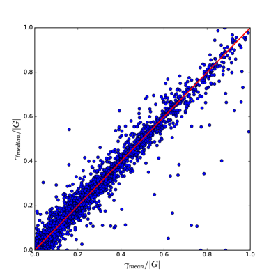
Figure 1: Scatter plot of the relative collective errors $\gamma_{mean}/|G|$ and $\gamma_{median}/|G|$. The solid line is the diagonal $\gamma_{mean}/|G|=\gamma_{median}/|G|$. Pearson’s correlation coefficient is $r=0.98$. Each symbol stands for one of the $15455$ forecasting contests, but not all contests are shown: the upper ranges of the $x$ and $y$ axes were limited to 1 to aid visualization, so about 3 percent of the forecasting contests are not represented in the figure.

To introduce the median we need to define the empirical cumulative distribution function Wasserman2004

$$F_{n}(g)=\frac{1}{n}\sum_{i=1}^{n}I(g_{i}\leq g)$$ (6)

where the indicator function is $I(g_{i}\leq g)=1$ if $g_{i}\leq g$ and $0$ otherwise. The median is then given by

$$F_{n}^{-1}(1/2)=\inf\{g:F_{n}(g)>1/2\}$$ (7)

where $F_{n}^{-1}(q)$ with $q\in[0,1]$ is the empirical quantile function, i.e., the inverse of the empirical distribution function. The collective error resulting from the use of the median to aggregate the individuals’ estimates is then

$$\gamma_{median}=|F_{n}^{-1}(1/2)-G|.$$ (8)

Figure 1 shows the scatter plot of the relative collective errors calculated with the mean and the median, as defined in equations (2) and (8), respectively. As expected, there is a high correlation between these two errors, viz., Pearson’s correlation coefficient is $r=0.98$. The median beats the mean in 50.4 percent of the forecasting contests. Note the outliers with large $\gamma_{mean}$ but small $\gamma_{median}$ that exemplify the robustness of the median to extreme individual estimates.

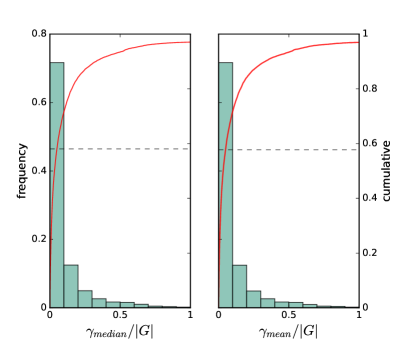
Figure 2: Histograms of the relative collective error calculated with the median $\gamma_{median}/|G|$ (left panel) and of the relative collective error calculated with the mean $\gamma_{mean}/|G|$ (right panel). The red curves are the cumulative distributions and the horizontal dashed lines indicate the value of the cumulative distribution when the relative collective error is $0.05$.

To offer more quantitative information on the data shown in the scatter plot, Fig. 2 exhibits the histograms and the cumulative distributions of the number of forecasting contests with a given relative collective error. The histograms are practically identical for the two aggregation methods, median and mean. In fact, both methods yield relative errors less than $0.05$ in 58 percent of the forecasting contests, but their relative errors are greater than 0.1 in 28 percent of the forecasting contests. In addition, the mean of the relative collective error calculated with the mean is $0.20\pm 0.01$ and the mean of the relative collective error calculated with the median is $0.19\pm 0.01$. The cumulative distributions exhibited in this figure show that about 3 percent of the forecasting contests have relative collective errors greater than 1 and are left out of the histograms (as well as of the scatter plot of Fig. 1) for the sake of visual clarity. We stress, however, that the forecasting contests left out of Figs.  1 and 2 are not influential in leading to the better overall results for the median.) In sum, whereas the crowd performance is clearly distinguishable since 58 percent of its predictions yielded an error of 5 percent or less, it falls short of being miraculous since it errs by more than 10 percent in 28 percent of the forecasting contests. In view of these findings, it seems likely that selective attention has played a considerable role to secure the popularity of the wisdom of crowds.

Next, we measure the fraction of individuals’ estimates that beat the collective estimate for each forecasting contest. The results are presented in form of histograms and cumulative distributions in Fig. 3, where the height of the bars is the proportion of forecasting contests for which that fraction equals $\xi\in\left[0,1\right]$. As already pointed out, the median estimate is always better than the estimates of half of the participants at least, so there is no forecasting contest for which $\xi_{median}>0.5$. However, the mean estimate beats the majority of the participants in 67 percent of the forecasting contests only. This number is obtained by evaluating the cumulative distribution function at $\xi_{mean}=0.5$. The fraction of forecasting contests for which $\xi_{mean}=0$ is $0.015$ and the fraction for which $\xi_{median}=0$ is $0.026$. This is the situation where the crowd beats all participants. Therefore, if the performance criterion is beating most or all participants then the median should definitely be preferred over the mean as an aggregation method since it is by construction guaranteed to beat at least half of the participants and has almost double the chances of beating all them as compared with the mean.

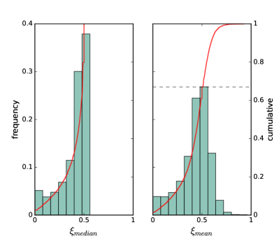
Figure 3: Histograms of the proportion of forecasting contests for which a fraction $\xi$ of the individuals’ estimates are more accurate than the relative collective estimate calculated with median (left panel) and the relative collective estimate calculated with the mean (right panel). The red curves are the cumulative distributions and the horizontal dashed line in the right panel indicates the value of the cumulative distribution at $\xi_{mean}=0.5$.

IV Testing the unbiased estimates assumption

As pointed out, a rather natural explanation for the wisdom of crowds assumes that the individuals’ estimates are unbiased, that is, that the errors spread in equal proportion around the correct value of the unknown quantity. Amusingly, if this assumption were correct one might harvest the benefits of the wisdom of crowds by asking a single individual to make several estimates at different times (see, e.g., Vul2008 ). Of course, the almost insurmountable difficulty to ensure that a same individual produces a large number of independent estimates of a same quantity makes the direct validation of the unbiased estimates assumption unfeasible. However, we can perform a much simpler and more informative test, viz., to check whether there is a meaningful correlation between the (unsigned) asymmetry of the distribution of individuals’ estimates and the collective error. In fact, according to the unbiased estimates assumption, the more asymmetric the distribution of estimates is, the more unlikely that the errors cancel each other out and hence the greater the collective error.

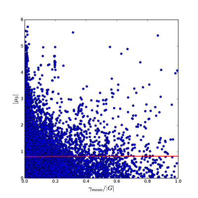
Figure 4: Scatter plot of the relative collective error $\gamma_{mean}/|G|$ calculated with the mean and the unsigned skewness $|\mu_{3}|$. The solid line is the linear regression. The Pearson correlation coefficient is $r=0.03$. The upper range of the $x$ axis was limited to 1 to aid visualization, but about 3 percent of the forecasting contests have relative errors greater than 1.

We recall that the skewness $\mu_{3}$ of a distribution is a dimensionless measure of its asymmetry defined as

$$\mu_{3}=\frac{1}{n}\sum_{i=1}^{n}\left(\frac{g_{i}-\langle g\rangle_{n}}{\delta^{1/2}}\right)^{3},$$ (9)

where $\langle g\rangle_{n}$ is the mean of the individuals’ estimates defined in equation (1) and $\delta$ is the sample variance of those estimates defined in equation (4). A negative value of $\mu_{3}$ implies that the left tail of the distribution of individual estimates is longer than the right tail, whereas a positive $\mu_{3}$ indicates a right-tailed distribution. Since the skewness $\mu_{3}$ measures the asymmetry with respect to the mean, in this analysis we will only consider the case that the collective estimate is calculated using the mean of the individuals’ estimates.

Figure 5: Histogram of the skewness $\mu_{3}$ of the distributions of individuals’ estimates. The wisdom of crowds experiments produce left- and right-tailed distributions in approximately the same proportion.

In Fig. 4 we show the scatter plot of the relative collective error calculated with the mean and the unsigned skewness. The results clearly contradict the unbiased estimates assumption, since they indicate that there is no meaningful correlation between the asymmetry of the distribution of individuals’ estimates and the collective error. More pointedly, Pearson’s correlation coefficient for these two variables is $r=0.03$ and the linear regression is $|\mu_{3}|\approx 0.81$. Particularly conspicuous are the great number of forecasting contests with high asymmetry and low prediction error, as well as with low asymmetry and high prediction error, that produce the triangle-shaped spreading of points depicted in Fig. 4. It is worth to mention here that if one were to expect that the estimates of a particular individual were unbiased, i.e., that they fluctuated symmetrically around the truth, that individual should most certainly be an expert on the matter in question. Hence our claim that the asymmetry of the distributions of the experts’ predictions in the FRBP database debunks the unbiased estimates assumption as an explanation for the accuracy of the crowd’s predictions.

Figure 5 shows that the distribution of the skewness is approximately symmetric, i.e., the number of right- and left-tailed distributions of individuals’ estimates are roughly the same in the forecasting contests of the FRBP database. Hence the asymmetry of those distributions has no role on the wisdom of crowds phenomenon. In fact, a scatter plot of the (signed) skewness against $\gamma_{mean}/|G|$ yields an almost perfectly symmetric distribution of points around $\mu_{3}=0$ (data not shown).

V Assessing the accuracy of the forecasters and the crowd

Figure 6: Scatter plot of the relative error of the ARIMA model $\gamma_{ARIMA}/|G|$ and the relative mean individual error $\epsilon/|G|$. The solid line is the diagonal $\gamma_{ARIMA}/|G|=\epsilon/|G|$. The upper ranges of the $x$ and $y$ axes were limited to 1 to aid visualization, but about 4 percent of the forecasting contests have relative errors greater than 1.

Our previous analysis yielded that the crowd errs by less than 5 percent in 58 percent of the forecasting contests, regardless of the method - mean or median - used to aggregate the participants’ estimates. Here we address the question: how good is this performance? Since the crowd beats all participants, which are all expert economists, in less than 3 percent of the forecasting contests, perhaps an error of 5 percent is nothing to boast about. Actually, we could as well ask: How good are the expert predictions, anyway? Of course, to answer those questions we must specify a standard of comparison. The seminal work of Meehl in the 1950s that made the astonishing claim that well-informed experts predicting outcomes were not as accurate as simple algorithms Meehl1954 (see also Tetlock2016 ) offers a clue. So here we use the basic ARIMA (AutoRegressive Integrated Moving Average) model, which is widely used in fitting and forecasting nonstationary time series Chatfield2000 ; Hyndman2018 , as the comparison standard to assess the goodness of both forecasters’ and crowd’s predictions.

The time series for a fixed variable, say NGDP, is the list of its true values $G$ for each month since the date the variable was included in the FRBP survey. We used the 12 values of the variable before the moment of the prediction to set the optimum parameters of the ARIMA model. In other words, we train the ARIMA model using a 12-quarters moving window. Once the ARIMA model is trained, we use it to predict the values of the variable at the five quarters subsequent to the moment of the prediction, similarly to what is asked to the participants of the FRBP-SPF. Since a fraction of the data of the FRBP-SPF database is used to train the ARIMA model, the number of forecasts used in this section is reduced to $13893$.

Let us first assess the accuracy of the individual forecasters. To achieve that we introduce the mean individual error

$$\epsilon=\frac{1}{n}\sum_{i=1}^{n}|g_{i}-G|,$$ (10)

which can be interpreted as the expected error of an expert selected at random among the $n$ participants of the forecasting contest. Figure 6 shows the scatter plot of the relative error of the ARIMA model $\gamma_{ARIMA}/|G|$ and the relative mean individual error $\epsilon/|G|$ for the $13893$ forecasting contests. We find that the ARIMA model is more accurate than a randomly selected expert in $35$ percent of the forecasting contests. The average relative mean individual error is $0.22\pm 0.01$ and the mean relative error of the ARIMA model is $0.31\pm 0.01$. Hence, at least in economics, the experts have a considerable advantage over simple time series forecasting algorithms.

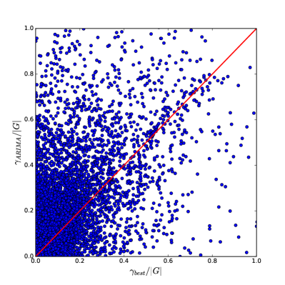
Figure 7: Scatter plot of the relative error of the ARIMA model $\gamma_{ARIMA}/|G|$ and the relative collective error $\gamma_{best}/|G|$. The solid line is the diagonal $\gamma_{ARIMA}/|G|=\gamma_{best}/|G|$. The upper ranges of the $x$ and $y$ axes were limited to 1 to aid visualization, but about 4 percent of the forecasting contests have relative errors greater than 1.

Next we compare the performance of the ARIMA model with the crowd’s performance, which for this analysis we define as $\gamma_{best}=\min\{\gamma_{mean},\gamma_{median}\}$. The results are actually insensitive to this definition because the accuracies of the median and the mean are very close (see Figs. 1 and 2). Figure 7 shows the scatter plot of the relative error of the ARIMA model $\gamma_{ARIMA}/|G|$ and the relative collective error $\gamma_{best}/|G|$. The ARIMA model beats the crowd in 28 percent of the forecasting contests. We recall that the mean relative error of the crowd is $0.19\pm 0.01$ and the mean relative error of the ARIMA model is $0.31\pm 0.01$.

An alternative way to assess the goodness of the crowd’s predictions is to compare them with the individual predictions that were closest to the true values, viz., the winning predictions of the forecasting contests. We have already pointed out that the odds that the crowd beats the winner is $0.015$ when the aggregate of the individuals’ estimates is the mean and $0.026$ when it is the median. Here we add that the mean relative error of the winners is $0.15\pm 0.01$, so the crowd performance as measured by its mean relative error is really not too far from the best the experts can offer.

VI Conclusion

The notion that a group of cooperating individuals can solve problems more efficiently than when those same individuals work in isolation is hardly contentious Rendell2010 , although the factors that make cooperation effective still need some straightening out Fontanari2014 ; Reia2019 . In fact, cooperation may well lead the group astray resulting in the so-called madness of crowds, as pointed out by MacKay almost two centuries ago MacKay1841 : “Men, it has been well said, think in herds; it will be seen that they go mad in herds, while they only recover their senses slowly, and one by one”. Less dramatically, cooperation may simply undermine the benefits of combining independent forecasts, which is known as the wisdom of crowds Lorenz2011 ; King2011 .

More precisely, the wisdom of crowds is the idea that the aggregation of the predictions of many independently deciding individuals is likely to be more accurate than the predictions of most or even all individuals within the crowd Surowiecki2004 . Here we use the Federal Reserve Bank of Philadelphia’s Survey of Professional Forecasters (FRBP-SPF) to offer an extensive statistical appraisal of the wisdom of crowds for the prediction of economic indicators. This approach is immune to the selective attention fallacy that has most likely influenced the anecdotal evidences for the wisdom of crowds that abound in the literature Nobre2020 . In addition, by focusing on the predictions of experts only we are in fact probing the so-called Vox Expertorum Coste1907 , which is the relevant voice when the forecasts address economic, social and political issues.

Our analysis of more than ten thousand forecasting contests reveals a noteworthy performance of the crowd, but that can hardly justify the ado about its wisdom. In particular, the odds that the crowd beats all participants of a forecasting contest is $0.015$ when the mean is used to aggregate the individuals’ estimates and $0.026$ when the aggregation is given by the median. This means that the crowd’s performance in Galton’s weighing contest, for which the mean collective estimate has zero error Wallis2014 , was quite atypical. The median has clear advantages over the mean as the method to combine the individuals’ estimates, specially when the crowd’s performance is compared with the participants’. In particular, the median is always guaranteed to beat at least half of the participants, whereas the mean beats the majority of the participants in 67 percent of the forecasts only (see Fig. 3) and, as just pointed out, the median has almost double the chances to beat all participants as compared to the mean.

Regarding the accuracy of the predictions, however, the advantage of the median is not so noticeable: it is more accurate than the mean in $50.4$ percent of the forecasts. The mean relative errors of both aggregation methods are around $20$ percent, which is not really bad considering that the mean relative error of the winners is $15$ percent and of a standard prediction algorithm (ARIMA) is $31$ percent. It is worth mentioning that the expected error of a randomly chosen forecaster is $22$ percent, so the participants of the FRBP survey predict better than the ARIMA on the average.

Another significant result of our extensive statistical analysis of the wisdom of crowds is the debunking of the unbiased estimates assumption, which purports to explain the accuracy of the crowd by assuming that the individuals’ judgments scatter symmetrically around the true value. If this were correct we should find a strong correlation between the asymmetry of the distribution of the individuals’ estimates and the error of the crowd’s estimate. We find no meaningful correlation between these two quantities (viz., Pearson correlation coefficient is $r=0.03$) and, in fact, there is a large number of forecasting contests with high asymmetry and low collective error (see Fig. 4). Because the large number of forecasting contests used in our analysis, the $p$-values associated to the correlation coefficients are extremely small, so all correlations reported in this paper are statistically significant. Their meaningfulness, however, is determined by the magnitude of the correlation coefficient $r$.

Our study of the wisdom of crowds dovetails with Quetelet’s original proposal of Social Physics as an empirical science Stigler2002 ; Donnelly2015 , where the regularities of the patterns observed in human behavior and refined through a statistical analysis are interpreted as the laws of the society (see also Perc2019 ). Perhaps, the statistical features reported here for the prediction of economic indicators hold true for the prediction of other continuous-valued quantities as well and so they may shed light on how (expert) humans estimate unknown quantities.

- (1) Galton F. Vox Populi. Nature 1907; 75(1949): 450–451.
- (2) Wallis KF. Revisiting Francis Galton’s Forecasting Competition. Statist Sci. 2014; 29(3): 420–424
- (3) Surowiecki J. The Wisdom of Crowds: Why the Many Are Smarter than the Few and How Collective Wisdom Shapes Business, Economies, Societies, and Nations. Doubleday; 2004.
- (4) Sunstein C. Infotopia: How Many Minds Produce Knowledge. Oxford University Press; 2006.
- (5) Page SE. The Difference: How the Power of Diversity Creates Better Groups, Firms, Schools, and Societies. Princeton University Press; 2007.
- (6) Lorenz J, Rauhut H, Schweitzer F, Helbing D. How social influence can undermine the wisdom of crowd effect. Proc Natl Acad Sci USA. 2011; 108(22): 9020–9025.
- (7) Bates JM, Granger CWJ. The combination of forecasts. Oper Res Q. 1969; 20(4): 451–468.
- (8) Nash UW. The Curious Anomaly of Skewed Judgment Distributions and Systematic Error in the Wisdom of Crowds. PLoS ONE 2014; 9(11): e112386.
- (9) Nash UW. Sequential sampling, magnitude estimation, and the wisdom of crowds. J. Math. Psychol. 2017; 77: 165–179.
- (10) Reia SM, Fontanari JF. Wisdom of crowds: much ado about nothing. J Stat Mech. 2021; 2021: 053402.
- (11) Nobre DA, Fontanari JF. Prediction diversity and selective attention in the wisdom of crowds. Complex Syst. 2020; 29(4): 861–875.
- (12) Federal Reserve Bank of Philadelphia. https://www.philadelphiafed.org/research-and-data/real-time-center/survey-of-professional-forecasters; 2022.
- (13) Clements MP, Rich RW, Tracy JS. Surveys of Professionals. Working Paper No. 22-13. Federal Reserve Bank of Cleveland; 2022. https://doi.org/10.26509/frbc-wp-2022-13.
- (14) King AJ, Cheng L, Starke SD, Myatt JP. Is the true ‘wisdom of the crowd’ to copy successful individuals? Biol Lett. 2011; 8(2): 197–200.
- (15) Perry-Coste FH. The ballot-box Nature 1907; 75(1952): 509.
- (16) Tan P-N, Steinbach M, Kumar V. Introduction to Data Mining. Pearson Education Limited; 2014.
- (17) Wasserman L. All of Statistics: A Concise Course in Statistical Inference. Springer; 2004.
- (18) Vul E, Pashler H. Measuring the crowd within: Probabilistic representations within individuals. Psychol Sci. 2008; 19(7): 645–647.
- (19) Meehl P. Clinical Versus Statistical Prediction. University of Minnesota Pres; 1954.
- (20) Tetlock PE, Gardner D. Superforecasting: The Art and Science of Prediction. Crown Publishing Group; 2016.
- (21) Chatfield C. Time-series forecasting. CRC Press; 2000.
- (22) Hyndman RJ, Athanasopoulos G. Forecasting: principles and practice. OTexts; 2018.
- (23) Rendell L, Boyd R, Cownden D, Enquist M, Eriksson K, Feldman MW, Fogarty L, Ghirlanda S, Lillicrap T, Laland KN. Why Copy Others? Insights from the Social Learning Strategies Tournament. Science 2010; 328(5975): 208–213.
- (24) Fontanari JF. Imitative Learning as a Connector of Collective Brains. PLoS ONE 2014; 9(10): e110517.
- (25) Reia SM, Amado AC, Fontanari JF. Agent-based models of collective intelligence. Phys. Life Rev. 2019; 31: 320–331.
- (26) MacKay C. Extraordinary Delusions and the Madness of Crowds. Richard Bentley; 1841.
- (27) Stigler SM. Statistics on the Table: The History of Statistical Concepts and Methods: The History of Statistical Concepts and Methods. Harvard University Press; 2002.
- (28) Donnelly K. Adolphe Quetelet, Social Physics and the Average Men of Science, 1796-1874. University of Pittsburgh Press; 2015.
- (29) Perc M. The social physics collective. Sci. Rep. 2019; 9:16549.