TESS Observations of Kepler systems with Transit Timing Variations

Abstract

We identify targets in the Kepler field that may be characterized by transit timing variations (TTVs) and are detectable by the Transiting Exoplanet Survey Satellite (TESS). Despite the reduced signal-to-noise ratio of TESS transits compared to Kepler, we recover 48 transits from 13 systems in Sectors 14, 15, 26, 40 and 41. We find strong evidence of a nontransiting perturber orbiting Kepler-396 (KOI-2672) and explore two possible cases of a third planet in that system that could explain the measured transit times. We update the ephemerides and mass constraints where possible at KOI-70 (Kepler-20), KOI-82 (Kepler-102), KOI-94 (Kepler-89), KOI-137 (Kepler-18), KOI-244 (Kepler-25), KOI-245 (Kepler-37), KOI-282 (Kepler-130), KOI-377 (Kepler-9), KOI-620 (Kepler-51), KOI-806 (Kepler-30), KOI-1353 (Kepler-289) and KOI-1783 (Kepler-1662).

1 Introduction

Transit timing has been of extraordinary value in characterizing the masses of exoplanets. Before the launch of the Transiting Exoplanet Survey Satellite ((TESS;) Ricker et al., 2015), the majority of low-mass exoplanets with measured sizes and masses were among multitransiting systems characterized by observed transit timing variations (TTVs; Hadden & Lithwick 2014; Jontof-Hutter et al. 2016; Hadden & Lithwick 2017; Jontof-Hutter 2019; Jontof-Hutter et al. 2021. These are due to coherent interactions between planets that cause measurable deviations from a constant orbital period (e.g., Agol et al., 2005; Holman & Murray, 2005; Ford et al., 2011; Fabrycky et al., 2012; Mazeh et al., 2013; Steffen et al., 2013). This windfall accrued from a combination of theoretical advances (Nesvorný & Morbidelli 2008; Nesvorný 2009; Lithwick et al. 2012; Agol & Deck 2016) and the abundance of compact multitransiting systems discovered by the Kepler mission (Lissauer et al. 2011a; Ford et al. 2012; Fabrycky et al. 2014).

The signal-to-noise ratio (S/N) of TTVs increases with orbital period, which biases planetary mass detections to longer orbital periods if long-baseline light curves are taken (Steffen, 2016). Hence, the Kepler mission (Borucki et al., 2010), with its 4 yr near-continuous photometric observations, enabled the majority of low-mass exoplanet characterizations to date. Such characterizations require both interacting neighbors to be transiting to enable planetary masses and radii to be measured. Near first-order mean motion resonances, where orbital periods $P_{in}$ and $P_{out}$ are near the ratio $j:j-1$ for an integer $j$, the TTVs are dominated by a sinusoidal signal of periodicity given by

$$P_{ttv}=\left|\frac{j-1}{P_{in}}-\frac{j}{P_{out}}\right|^{-1}$$ (1)

The majority of TTV mass characterizations are among compact multiplanet systems in the Kepler field, where TTVs are detected at the expected TTV periodicity (or super-period) given the orbital periods of the planets (Lithwick et al. 2012; Hadden & Lithwick 2014).

Both the TTV periodicity and the amplitude of the signal increase as the orbital period ratio approaches commensurability (Lithwick et al., 2012). This adds value to increasing the baseline of photometric observations. Some Kepler targets with TTVs are detectable from ground-based observatories (von Essen et al., 2018). However, due to the long orbital periods and long transit durations of many of the most interesting systems, ground-based transit timing is inefficient. In some cases, only one of ingress or egress is recoverable in one night (e.g., Dalba & Muirhead, 2016). In addition, some of the candidates with long orbital periods have few transits during the season when the Kepler field is observable.

Nevertheless, additional data can significantly improve the constraints of TTV models. Arguably, the most valuable follow-up data are where the periodicity of a large TTV signal is comparable to or exceeds the Kepler baseline (e.g. Kepler-29 and Kepler-177; Vissapragada et al. 2020).

TESS solves some of the problems of ground-based follow-up with its 27-day sectors. So long as a target transits within the relevant time frame, its ingress and egress will likely be covered, enabling precise mid-transit timing measurements. To date, TESS has observed the Kepler field in part or in whole in Sectors 14, 15, 26, 40, and 41. TESS may provide useful transit photometry for a significant number of planets even though the transit S/N is much lower than in the Kepler data set. These may improve planetary mass measurements and refine ephemerides (Battley et al., 2021).

Our aim is to identify targets among Kepler’s multiplanet systems where there are known TTVs or an expectation of TTVs such that TESS data may further characterize planetary masses and orbital parameters. In this section, we compile a list of TTV targets in the Kepler field where there is an expectation of detecting a transit in TESS data. In §2, we explain our light curve analysis and results, including our measured transit times. In §3, we present our analysis of measured transit times alongside Kepler data and characterize the planetary parameters. We discuss the results in §4.

1.1 System Selection

We identified planets with known TTVs according to the transit timing catalog of Holczer et al. (2016), and from this sample we selected for planets within multitransiting systems where the TTVs could be attributable to an interacting neighbor near a first-order or second-order mean motion resonance. For this, we calculated the period ratios of all adjacent planet pairs and the period ratios of nonadjacent planet pairs with one intermediate transiting planet from Kepler’s multitransiting systems. We considered planet pairs to be near first-order resonance if the period ratio fell within a range bounded by the nearest third-order resonances to the first-order resonance. Outside of this domain, we considered period ratios up to 4:1 as nearer to second-order resonances. We excluded pairs with period ratios greater than 4:1, since their interactions are unlikely to cause any observed TTVs. These were at KOI-289, KOI-353, KOI-464, KOI-564, KOI-872, KOI-1781 and KOI-1792. These systems have detectable TTVs, but the known planets are likely noninteracting and hence TTV modeling will not characterize the masses of the transiting planets. These are distinct from systems where prior studies have considered the known planets to be sufficient for TTV modeling, but additional information from TTV or radial velocity (RV) implies the presence of nontransiting perturbers (see §3.3).

We also excluded KOI-676 which has a pair near the 13:4 commensurability. The TTVs detected by Holczer et al. (2016) at the inner planet, KOI-676.01, are most likely caused by a nontransiting perturber.

In addition to the TTV systems identified by Holczer et al. (2016), we added planets with an expected TTV periodicity $>$100 days that have no prior detection of TTVs. The TTV signals of planet pairs near first-order resonances are generally dominated by a single periodicity, given by Equation 1. Among pairs near second-order resonances, TTV signals have more components. For a period ratio near $j:j-2$, we calculated a periodicity that satisfies

$$\frac{1}{P_{ttv}}=\left|\frac{j-2}{P_{in}}-\frac{j}{P_{out}}\right|.$$ (2)

We determined which of these planet candidates were likely detectable in TESS light curves at the 3$\sigma$ level as follows. For a given planet transit depth $\delta_{p}$ and transit duration in hours, $T_{dur}$, we anticipated that

$$S/N_{TESS}\approx\frac{\delta_{p}\sqrt{T_{dur}}}{\delta_{\rm{1\>hr}}}$$ (3)

where $\delta_{\rm{1\>hr}}$ is the TESS uncertainty for a 1 hr observation of the target estimated using the Web TESS Viewing Tool. We adopted the transit depth and duration measurements from Kepler DR25 for this calculation (Thompson et al., 2018). KOI-377.02 was excluded from DR25, and we adopted the values from Mullally et al. (2015).

Finally, from this list we selected targets where transits were expected in the TESS sectors. Our targets are in Table 1.

KOI	P (days)	$\delta$ (ppm)	TESS $\delta_{\rm{1\>hr}}$	Tdur (hr)	Exp. S/NTESS	Pttv (days)
94.01	22.343	5610	526.9	6.66	27.5	156
94.02	10.424	777	526.9	5.23	3.4	156
94.03	54.320	1980	526.9	8.59	11.0	126
137.01	7.642	2270	1270.2	3.41	3.3	268
137.02	14.859	3270	1270.2	3.53	4.8	268
152.01	52.091	2890	1618.7	8.64	5.2	721
244.01	12.720	1180	245.2	2.73	8.0	326
244.02	6.239	402	245.2	3.53	3.1	326
282.01	27.509	639	428.9	5.93	3.6	482
377.01	19.271	6661	1424.0	4.13	9.5	$\approx$ 2000
377.02	38.908	6159	1424.0	4.52	9.2	$\approx$ 2000
620.01	45.155	6210	2691.8	5.78	5.5	1112
620.02	130.178	11600	2691.8	8.45	12.5	$\approx$ 2500
806.01	143.206	10600	4712.5	8.93	6.7	383
806.02	60.325	20300	4712.5	6.62	11.1	383
1353.01	125.865	12400	1786.0	9.02	20.9	874
1426.02	74.928	4120	1880.2	4.74	4.8	$\approx$ 70,000
1426.03	150.019	4320	1880.2	4.38	4.8	$\approx$ 70,000
1783.01	134.479	4030	1694.7	5.93	5.8	$\approx$ 2500
2672.01	88.512	2520	421.0	6.82	15.6	1506
2672.02	42.992	1120	421.0	4.73	5.8	1506
70.01	10.854	1030	590.8	3.78	3.4	171
82.01	16.146	941	318.1	3.72	5.7	123
245.01	39.792	610	135.9	4.47	9.5	302
351.01	331.597	8320	1470.1	14.40	21.5	$\approx$ 2200
351.02	210.601	4160	1470.1	11.99	9.8	$\approx$ 2200

Table 1: Selected KOIs for Transit Timing with TESS. Note. The columns list the KOI, orbital period in days, nominal transit depth (from DR 25), estimated 1 hr photometric precision with TESS, nominal transit duration in hours, expected transit S/N and expected TTV period in days. The top section lists candidates with known TTVs from Holczer et al. (2016). The bottom section lists additional candidates with an expected TTV period $>$100 days.

Most of these targets were anticipated by prior authors (e.g. Christ et al. 2019; Goldberg et al. 2019). Beyond targets identified by Christ et al. (2019), our criteria for inclusion adds planets at KOI-245 (Kepler-37), KOI-282 (Kepler-130), KOI-351 (Kepler-90), KOI-1353 (Kepler-289) and KOI-1783 (Kepler-441).

2 Observations

To date, TESS has observed the Kepler field during Sectors 14, 15, 26, 40, and 41. Kepler’s TTV systems received different baselines of observation based on their position relative to TESS’s pointing and the location of CCD gaps. For the systems that were observed for at least one sector, we accessed the target pixel file (TPF) data from the Mikulski Archive for Space Telescopes through the lightkurve package (Lightkurve Collaboration et al., 2018). TPF data are background-subtracted cutouts with the electron flux in the pixels containing and surrounding the target star (Jenkins et al., 2016). Most Kepler TTV systems were observed with 2-minute cadence under the Cycle 2 TESS Guest Investigator Program G022149 (PI: Jontof-Hutter). In several cases, a system did not receive 2-minute cadence owing to its proximity to the edge of the detector.

2.1 Trapezoidal Transit Modeling with Pixel-level Decorrelation

The TESS mission has an emphasis on bright, nearby star systems (Ricker et al., 2015). Many of the Kepler TTV systems, on the other hand, are relatively faint and distant. Therefore, in many cases, the anticipated transit depths for our Kepler host stars are on the order of the uncertainty in their relative flux measurements from TESS. This presents a critical challenge to measuring the TESS transit times, and hence a careful treatment of the noise in the TESS photometry is warranted.

We employ pixel-level decorrelation (PLD; Deming et al., 2015) to simultaneously model the noise and the transit in the TESS photometry. PLD has been successfully used to model instrumental systematics in light curves stemming from motion of the stellar point-spread function (PSF) and intrapixel sensitivity variations (Ingalls et al., 2012; Deming et al., 2015; Luger et al., 2016). In PLD, the systematic intensity variations are modeled by treating the individual pixel light curves as basis vectors, which are obtained by applying a normalization to remove the noninstrumental signal and linearly combined, i.e.,

$$M_{\mathrm{PLD}}^{t}(\boldsymbol{\alpha})=\frac{\sum_{i=1}^{n}c_{i}P_{i}^{t}}{\sum_{i=1}^{n}P_{i}^{t}},$$

where $M_{\mathrm{PLD}}$ is the PLD model (parameterized by $\boldsymbol{\alpha}$) at time $t$, the $P_{i}$ are the pixel light curves, and the $\boldsymbol{\alpha}=\{c_{1},c_{2},...,c_{n}\}$ are the parameters of the PLD model; the number of basis vectors $n$ is determined by the number of pixels in the optimal TESS aperture.

PLD was initially designed to account for noise in light curves from the Spitzer Space Telescope (Deming et al., 2015). It is similarly applicable to TESS observations in which large pixels undersample the stellar PSF. The PLD coefficients are fit to the data simultaneously with the parameters of the trapezoidal transit model, thus allowing for error propagation. In the following explanation of our methods, we will show the data from the Kepler-396 system as a representative example of the full population of Kepler TTV systems.

For each target in each sector it was observed, we begin by identifying the pixels in the default photometric aperture as calculated by the Science Processing Operations Center (SPOC) data pipeline (Jenkins et al., 2016). The TPF for Kepler-396 from Sector 15 generated with the tpfplotter tool (Aller et al., 2020) is shown in Figure 1. We inspected the aperture for dilution from nearby stars known to exist in the Gaia DR2 catalog (Gaia Collaboration et al., 2018). In a few cases, we altered the default aperture to reduce contamination from background stars, especially if the transit depth we measured was much shallower than expected.

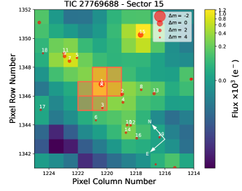
Figure 1: TPF for Kepler-396 from Sector 15 generated with tpfplotter (Aller et al., 2020). The numbered red circles are background stars identified by Gaia with size corresponding to the magnitude difference compared to Kepler-396 (marked with a cross and numbered “1”). The red squares identify the pixels in our custom aperture, which minimizes contamination from a nearby source. These pixels’ light curves—normalized to their sum—formed the set of basis vectors for the PLD analysis of this system.

After masking data during the expected transit time, we identified and removed outlier cadences from the TPF time series by generating a light curve using the default aperture photometry setting in lightkurve. For most systems, we trimmed the data to only include cadences within $\pm$0.5 days of the expected transit. This window was extended in a few cases (including Kepler-396 c) to allow for larger-than-expected TTVs. We then extracted the raw, background-subtracted light curves in each pixel using our photometric aperture. We normalized these light curves to their sum such that each cadence summed to unity. We also included an additional basis vector that was a linearly increasing function of time. The linear combination of the normalized basis vectors, weighted by coefficients $c_{i}$, where $i$ denotes the $i$th pixel, produced the noise model for each star’s light curve. Since the aperture size varied by target and sector, the number of $c_{i}$ coefficients (and thus free parameters) was variable.

The S/N in TESS data for any transit of a KOI is much lower than the S/N in Kepler. Since low S/N is especially prohibitive of detecting limb darkening, we chose to model the transit signal with a simple four-parameter trapezoid model: $T_{C}$ is the mid-transit time, $\delta$ is the transit depth, $T_{14}$ is the total transit time (first to fourth contact), and $T_{23}$ is the full transit time (second to third contact). The trapezoidal representation of the transit represented a sensible balance between simplicity and functionality and allowed us to place priors on the duration of each transit.

2.2 Priors on Trapezoidal Transit Parameters

We placed a uniform prior on the mid-transit time of width $\pm$0.25 days from the projected transit times of Jontof-Hutter et al. (2021) where available, or an extrapolation to a linear fit to the Kepler transit times. In some cases (such as Kepler-396c) the window for a detection in the TESS light curve was increased to $\pm$1 day.

To detect the transits of known planets in TESS light curves, we imposed a strict prior on transit duration from Kepler data. Having a narrow prior on the duration of any transit meant that we did not generally improve on the duration measurements made from the Kepler data. However, given that our goal was to measure the mid-transit time and that the quality of the Kepler data for our faint targets always exceeded that of TESS, this was an acceptable choice.

Assuming low eccentricity, transit durations are given by

$$T_{23}=\frac{P}{\pi}\sin^{-1}\left[\frac{R_{\star}}{a}\frac{\sqrt{(1-k)^{2}-b^{2}}}{\sin i}\right]$$ (4)

and

$$T_{14}=\frac{P}{\pi}\sin^{-1}\left[\frac{R_{\star}}{a}\frac{\sqrt{(1+k)^{2}-b^{2}}}{\sin i}\right]$$ (5)

where $P$ is the orbital period, $R_{\star}/a$ is the radius of the star scaled by the orbital semi-major axis, $k=R_{p}/R_{\star}$, $b$ is the impact parameter, and $i=\cos^{-1}(bR_{\star}/a)$ is the inclination (Winn, 2010). For our trapezoidal transit fits, our free parameters were $T_{14}$ and the ratio the transit durations $f_{T}\equiv T_{23}/T_{14}$, with priors based on published measurements of $R_{\star}/a$, $k$ and $b$ with their reported uncertainties (assumed to be Gaussian) from Kepler DR25.

For asymmetric errors, we adopted the larger of the two as the width of our priors. However, in many cases impact parameters are reported with asymmetric errors, with effectively an upper bound as the only constraint. For these, we assumed a uniform distribution between zero and the implied “2$\sigma$” upper bound.

For example, DR25 reports the impact parameter of Kepler-25 c as $b=0.787^{+0.051}_{-0.401}$, suggesting that while the bounds are uncertain, Kepler-25 c has a high impact parameter, moderately inconsistent with zero. A uniform distribution between zero and the upper limit would thus give too much weight to low values for the impact parameter. However, Kepler DR24 (Coughlin et al., 2016) report $b=0.1062^{+0.2045}_{-0.1062}$. We note that TTVs could cause erroneously high estimates of impact parameter since stacking the transits would increase the inferred ingress and egress time in the combined light curve. This is unlikely to be a factor for Kepler-25 c since the TTVs have an amplitude less than 5 minutes and are insignificant compared to the transit duration of $\approx 2.7$ hr. For this planet, we adopted a uniform distribution up to the upper bound given by DR25.

Kepler-9 c (KOI-377.02) was not included in DR25 or DR24. We have adopted the relevant parameters from the Q1–Q16 Kepler catalog of Mullally et al. (2015).

In cases like KOI-94.03, where $R_{\star}/a$ is poorly constrained, we note that $(R_{\star}/a)^{3}<<1$ and adopt a leading-order approximation for the inverse sine function, in which the ratio:

$$\frac{T_{23}}{T_{14}}\approx\sqrt{\frac{(1-k)^{2}-b^{2}}{(1+k)^{2}-b^{2}}}$$ (6)

This eliminates the uncertainties from $R_{\star}/a$ and $\sin i$.

For KOI-1426.03, the impact parameter reported in DR25 $b=1.25^{+67.03}_{-0.17}$ is likely skewed by TTVs. This also affects the measured scaled planetary radius $k$. In estimating priors for transit duration, we assumed $k\approx\sqrt{\delta}$, and drew samples of $b\sim U[0,1]$.

For the PLD coefficients $c_{i}$, we allowed the sampler to explore all values between positive and negative infinity. Lastly, for transit depth $\delta$, we placed a uniform prior between 0 and 1. We generally did not attempt to correct for transit depth dilution except in a few cases in which we altered the photometric aperture.

2.3 Transit Recovery and Model Fitting

We added the trapezoid model to the noise model to construct the final model light curve, which we fit to the data using the emcee ensemble sampler (Foreman-Mackey et al., 2013). We initiated the fit with all PLD coefficients at zero and all transit parameters at the expected values based on Kepler DR25. We allowed 100 chains to explore the parameter space for 10,000 steps each for a total of $1\times 10^{6}$ evaluations. We determined the burn-in by visual inspection, finding 2000 steps to usually be more than enough time for the chains to identify the region of highest likelihood.

To illustrate our method for identifying and characterizing transit events in TESS data, we show our light-curve analysis for Kepler-396. In Figure 2, we show the full posterior distribution for all parameters modeled for Kepler-396 c. These posteriors are representative of other fits for which a clear transit detection was made. The posteriors for the PLD coefficients are normal distributions centered on zero. The transit duration parameters broadly follow their strict normal priors. The depth posterior is normal and well separated from zero. Lastly, the posterior for mid-transit time $T_{C}$ is unimodal and roughly normal, although it can be skewed as is the case for Kepler-396 c.

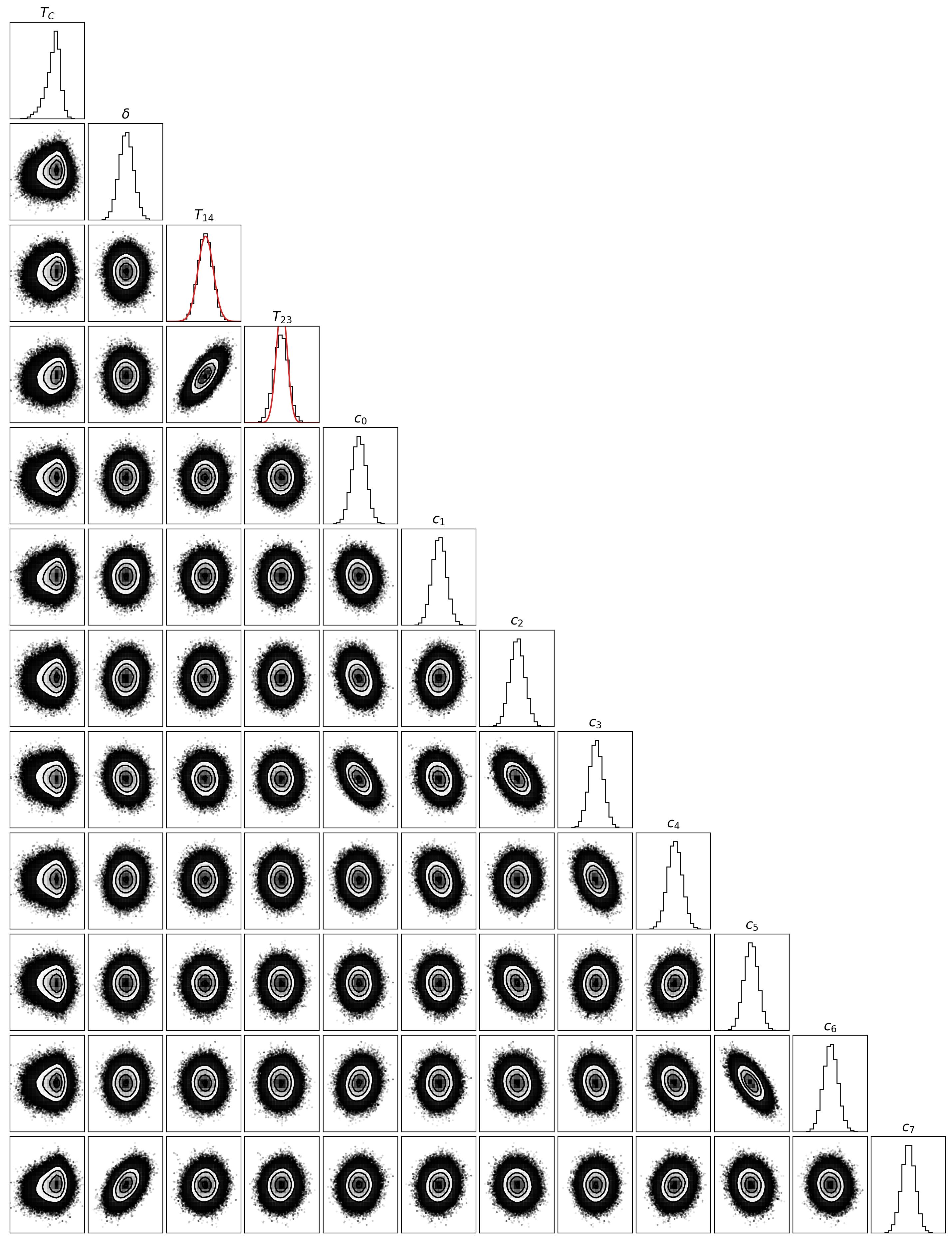
Figure 2: Posterior probability distributions for the PLD and trapezoidal transit fit to the Sector 15 Kepler-396 c transit. The first four columns are the trapezoid parameters, while the remaining columns are PLD basis vector coefficients. The red curves denote the normal priors on $T_{14}$ and $T_{23}$, the latter of which is transformed from the prior on $f_{T}$. These posteriors correspond to the fit shown in Figure 4.

In systems with weaker detections than shown for Kepler-396 c, the posterior on $T_{C}$ was usually broader, was less normal, and sometimes approached the edge of the uniform prior. In these cases, the depth posteriors were sometimes consistent with zero to $\sim 3\sigma$. In systems with nondetections, the depth posteriors were typically within $2\sigma$ of zero and the $T_{C}$ posterior was either multimodal or flat but spanned the entire width of the prior. In weak detections and nondetections, the posteriors of the PLD coefficients were always normal (i.e., we could always fit a noise model even if a transit could not be detected).

In Figures 3 and 4, we show the data and best-fit models for the three transits of Kepler-396 b in Sectors 14, 15, and 41 and the two transits of Kepler-396 c in Sectors 15 and 41. Each panel is centered on the expected mid-transit time. The Sector 15 transit of Kepler-396 c is clearly visible in the light curve and occurred substantially later than expected. The Sector 14 transit of Kepler-396 b is subtler and more representative of most other TTV systems that we modeled. Through the use of PLD, we are able to make an accurate measurement of this planet’s transit even though the depth is on the order of the scatter in the data. The Sector 15 transit of Kepler-396 b, however, is a representative example of marginal detection. The timing of the transit is uncertain owing to correlated noise in the data that is not entirely captured by the PLD model.

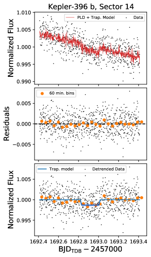
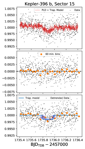
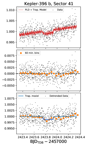
Figure 3: PLD and trapezoidal model fits to the three transits observed for Kepler-396 b. The top panel of each column shows normalized but not detrended flux from the default SPOC apertures. In each column, the data are centered on the expected transit timing based on TTV models of Kepler transit times for this system. The shaded region in the bottom panels shows the 68% credible region for the trapezoidal fits, with the median in bold. The credible region for Kepler-396 b is less constrained in Sector 15 owing to correlated noise that is poorly modeled by PLD.

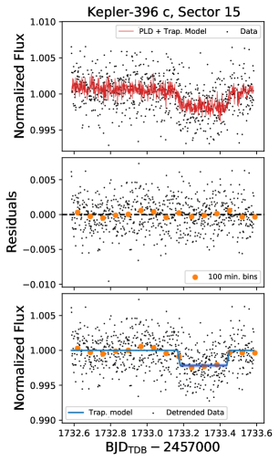
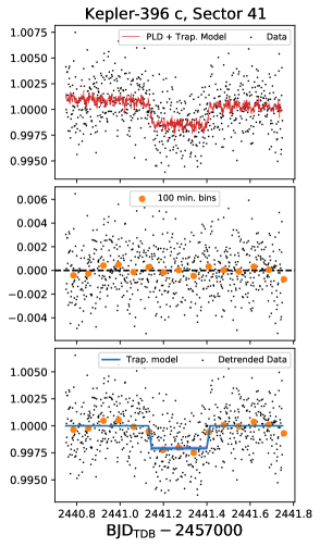
Figure 4: PLD and trapezoidal models fit to the two transits observed for Kepler-396 c. The style of this figure is identical to that of Figure 3. The Sector 15 transit occurs substantially later than expected.

In Tables 2,  3 and 4 we list all the transits that were sought from the TESS data. The majority of stars were observed with short (fast) cadence with exposures every 2 minutes. However, some stars were only observed with long (slow) cadence with exposures every 30 minutes. In the latter case, we accessed the full-frame image (FFI) data and manually chose photometric apertures to minimize contamination from background sources.

We required transit-like signatures to have a depth inconsistent with zero at the 2$\sigma$ level. In addition, despite our modeling of correlated noise, the risk remains of fitting low-S/N transits to noise features. We rejected the fitted central times of transit-like signatures that, by eye, appeared sensitive to residual correlated noise. The noise could affect the time of the transit model, in which the trapezoidal ingress or egress favors variations due to noise. In some cases we found low-S/N transits with mid-transit times that appear unlikely given the projected transit times following the Kepler data. In other cases, correlated noise caused multimodal transit timing posteriors.

The correlated noise can also affect the transit depth. We expect dilution to reduce the depth of transits in many TESS light curves compared to Kepler light curves of the same targets. Hence, we did not reject fits to TESS light curves with shallower transits. However, transits that were measured to be deeper than the Kepler model, while possible with different choices for apertures and background subtraction, are unlikely to be significant, and hence we rejected them as fitted red noise. KOI-137.02 (Kepler-18 d) is an exception to this. Our measured transit depth was 0.55$\%\pm 0.08\%$, significantly deeper than the Kepler DR25 measurement and discrepant at the 2.75$\sigma$ level. Kepler-18 is faint for a TESS target ($V=13.8$), and the flux in each pixel of the photometric aperture was on the order of the background signal. As a result, this system is especially sensitive to the background model, for which we used the SPOC pipeline default. The processed light curve for Sector 14 shows little evidence of time-correlated noise, and the transit is visible by eye at the expected time and with the expected duration. Since this light curve was particularly sensitive to background subtraction, we did not reject the strong detected signal due to its unexpected depth. Hence, we claim this transit as a detection.

In the case of KOI-137, the expected transits from planets c and d overlapped in Sector 15. We accounted for this by simultaneously fitting two trapezoid models with the duration priors of each planet. The result was a multimodal posterior to the mid-transit time for each planet, with transit depths that were larger than expected based on the Kepler data. Away from these transits, the light-curve residuals clearly exhibit time-correlated noise with features as large as or larger than the expected transits. For these reasons, we concluded that we were fitting noise features and claimed a nondetection for both transits.

Kep $\#$	KOI	Sect.	Pr. T14 (hr)	Pr. T23/T34	Pred. Time	Obs. Time	status
20c	70.01	14	3.78 $\pm$ 0.02	0.930 $\pm$ 0.004	1683.709 $\pm$ 0.002		R1
		14			1705.417 $\pm$ 0.002		R2
		26			2400.079 $\pm$ 0.002		R3
		26			2410.933 $\pm$ 0.002	2410.9509 ${}^{+0.026}_{-0.0087}$	A
		26			2421.787 $\pm$ 0.002	2421.6798 ${}^{+0.096}_{-0.0096}$	A
		26			2432.641 $\pm$ 0.002		R2
		26			2443.495 $\pm$ 0.002	2443.515 $\pm$ 0.021	A
102e	82.01	14	3.72 $\pm$ 0.03	0.931 $\pm$0.006	1697.407 $\pm$ 0.002	1697.416 ${}^{+0.021}_{-0.029}$	A
		26			2020.322 $\pm$ 0.003	2020.3142 ${}^{+0.0085}_{-0.018}$	A
		40			2391.673 $\pm$ 0.003	2391.678 $\pm$ 0.010	A
		40			2407.819 $\pm$ 0.003	2407.817 $\pm$ 0.025	A
		41			2423.963 $\pm$ 0.003		R4
		41			2440.109 $\pm$ 0.003		R4
89d	94.01	14	6.664$\pm$0.004	0.851$\pm$0.001	1697.0182 $\pm$ 0.0005		R1
		15			1719.3614 $\pm$ 0.0005	1719.3595 ${}^{+0.0063}_{-0.0071}$	A
		41			2434.3352 $\pm$ 0.0006	2434.3361 ${}^{+0.0041}_{-0.0037}$	A
89c	94.02	14	5.23 $\pm$ 0.02	0.942 $\pm$ 0.001	1692.2613 $\pm$ 0.0021	1692.2954 ${}^{+0.0091}_{-0.0053}$	A
		14			1702.6851 $\pm$ 0.0021	1702.685 ${}^{+0.017}_{-0.041}$	A
		15			1713.1120 $\pm$ 0.0023	1713.098 ${}^{+0.035}_{-0.010}$	A
		15			1723.5370 $\pm$ 0.0025	1723.569 ${}^{+0.041}_{-0.023}$	A
		15			1733.9636 $\pm$ 0.0026		R3
		41			2432.3459 $\pm$ 0.0029		R3
		41			2442.7679 $\pm$ 0.0030		R3
89e	94.03	14	8.59 $\pm$ 0.02	0.907 $\pm$ 0.002	1688.0025 $\pm$ 0.0021	1687.950 ${}^{+0.021}_{-0.018}$	A
18c	137.01	14	3.41 $\pm$ 0.01	0.914 $\pm$ 0.003	1689.8538 $\pm$ 0.0007		R3
		14			1697.4947 $\pm$ 0.0007		R4
		14			1705.1357 $\pm$ 0.0007		R4
		15			1712.7768 $\pm$ 0.0007	1712.761 ${}^{+0.014}_{-0.013}$	A
		15			1720.4178 $\pm$ 0.0007		R4
		15			1728.0587 $\pm$ 0.0007		R3
		15			1735.6996 $\pm$ 0.0007	1735.681 ${}^{+0.042}_{-0.016}$	A

Table 2: Transits Searched for and Recovered from TESS Sectors 14, 15, 26, 40, and 41: Part 1 of 3. Note. Priors in transit duration (Pr. T₁₄ and Pr. T₂₃/T₁₄; Columns (4) and (5)) correspond to the total duration from first to last contact, and the fraction of this duration in which the planet is entirely on the disk of the star respectively. The times listed in Column (6) are the predicted time following fits to Kepler data. Column (7) gives our measured transit time if it was detected. All times are in BJD$-$2,457,000. The last column lists whether we accepted the transit as a detection (A), or whether the transit was rejected for any of several reasons: a likely transit was totally or partially affected by a data gap (R1) the trapezoidal fit was a non-detection (R2), the posterior depth was consistent with zero (R3), or the fitted model appeared by inspection to be sensitive to correlated noise (R4). We note where short-cadence data were unavailable and we relied on FFIs (F).

Kep $\#$	KOI	Sect.	Prior T14 (hr)	Prior T23/T34	Pred. Time	Obs. Time	status
		40			2423.4433 $\pm$ 0.0009		R2 (F)
		41			2431.0857 $\pm$ 0.0009		R2 (F)
		41			2438.7275 $\pm$ 0.0009		R2 (F)
18d	137.02	14	3.53 $\pm$ 0.01	0.898 $\pm$ 0.004	1690.7417 $\pm$ 0.0007	1690.7457 ${}^{+0.0044}_{-0.0037}$	A
		14			1705.6013 $\pm$ 0.0008	1705.6112 ${}^{+0.0060}_{-0.0044}$	A
		15			1720.4610 $\pm$ 0.0008		R4
		15			1735.3209 $\pm$ 0.0008		R4
		41			2433.6879 $\pm$ 0.0009		R1
79d	152.01	14	8.64 $\pm$ 0.02	0.903 $\pm$ 0.002	1690.2027 $\pm$ 0.0041		R3
		41			2419.4699 $\pm$ 0.0044		R1
25c	244.01	14	2.73 $\pm$ 0.05	0.896 $\pm$ 0.049	1687.7166 $\pm$ 0.0006	1687.7126 ${}^{+0.0033}_{-0.0025}$	A
		14			1700.4368 $\pm$ 0.0006	1700.4451 ${}^{+0.0038}_{-0.0061}$	A
		40			2400.0563 $\pm$ 0.0007	2400.0483 ${}^{+0.0027}_{-0.0030}$	A
		40			2412.7763 $\pm$ 0.0007	2412.7788 ${}^{+0.0025}_{-0.0035}$	A
		40			2425.4964 $\pm$ 0.0007	2425.5071 ${}^{+0.0049}_{-0.0055}$	A
		41			2438.2165 $\pm$ 0.0007	2438.2144 ${}^{+0.0034}_{-0.0017}$	A
25b	244.02	14	3.53 $\pm$ 0.01	0.960 $\pm$ 0.004	1685.4406 $\pm$ 0.0016	1685.4358 ${}^{+0.017}_{-0.0055}$	A
		14			1691.6793 $\pm$ 0.0016		R2
		14			1697.9180 $\pm$ 0.0016	1697.9118 ${}^{+0.0061}_{-0.0038}$	A
		14			1704.1567 $\pm$ 0.0016	1704.1262 ${}^{+0.0079}_{-0.0092}$	A
		40			2390.3975 $\pm$ 0.0019		R2
		40			2396.6365 $\pm$ 0.0019	2396.546 ${}^{+0.026}_{-0.034}$	A
		40			2402.8754 $\pm$ 0.0019	2402.879 ${}^{+0.014}_{-0.036}$	A
		40			2409.1143 $\pm$ 0.0019		R2
		40			2415.3531 $\pm$ 0.0019		R2
		40			2421.5921 $\pm$ 0.0019		R2
		41			2427.8308 $\pm$ 0.0019		R2
		41			2434.0697 $\pm$ 0.0020		R2
		41			2440.3084 $\pm$ 0.0020		R2
		41			2446.5472 $\pm$ 0.0020		R1
37d	245.01	14	4.47 $\pm$ 0.02	0.947 $\pm$ 0.010	1708.9298 $\pm$ 0.0019	1708.9327 ${}^{+0.0037}_{-0.0031}$	A
		26			2027.2674 $\pm$ 0.0021	2027.270 ${}^{+0.016}_{-0.020}$	A (F)
		41			2425.1888 $\pm$ 0.0022	2425.1903 ${}^{+0.0039}_{-0.0033}$	A
130c	282.01	14	5.93 $\pm$ 0.04	0.930 $\pm$ 0.008	1701.2660 $\pm$ 0.0022		R2 (F)
		40			2416.4929 $\pm$ 0.0031	2416.4765 ${}^{+0.011}_{-0.0076}$	A
		41			2444.0019 $\pm$ 0.0031		R3
90g	351.02	40	11.99 $\pm$ 0.03	0.886 $\pm$ 0.005	2406.0349 $\pm$ 0.1228		R2 (F)

Table 3: Transits Searched for and Recovered from TESS Sectors 14, 15, 26, 40, and 41: Part 2 of 3. The format is the same as Table 2.

Kep $\#$	KOI	Sect.	Pr. T14 (hr)	Pr. T23/T34	Pred. Time	Obs. Time	status
9b	377.01	14	4.13 $\pm$ 0.01	0.858 $\pm$ 0.004	1691.9272 $\pm$ 0.0102		R2 (F)
		26			2018.8745 $\pm$ 0.0150		R2 (F)
		40			2403.2777 $\pm$ 0.0126	2403.3141 ${}^{+0.0020}_{-0.0018}$	A (F)
		41			2422.5023 $\pm$ 0.0124	2422.5392 ${}^{+0.0057}_{-0.0029}$	A (F)
		41			2441.7270 $\pm$ 0.0122	2441.666 ${}^{+0.036}_{-0.14}$	A (F)
9c	377.02	14	4.53 $\pm$ 0.04	0.743 $\pm$ 0.018	1708.4681 $\pm$ 0.0235		R3
		26			2020.6351 $\pm$ 0.0335		R2 (F)
		40			2411.3611 $\pm$ 0.0289	2411.4242 ${}^{+0.004}_{-0.049}$	A (F)
51b	620.01	14	5.78 $\pm$ 0.02	0.858 $\pm$ 0.007	1694.8509 $\pm$ 0.0023	1694.879 ${}^{+0.021}_{-0.011}$	A
51d	620.02	14	8.45 $\pm$ 0.02	0.815 $\pm$ 0.005	1689.9844 $\pm$ 0.0192	1689.996 ${}^{+0.023}_{-0.013}$	A
30d	806.01	41	8.93 $\pm$ 0.10	0.811 $\pm$ 0.018	2426.6872 $\pm$ 0.0045	2426.82${}^{+0.10}_{-0.18}$	A (F)
30c	806.02	14/15	6.62 $\pm$ 0.03	0.762 $\pm$ 0.009	1696.3701 $\pm$ 0.0011		R1
		41			2420.2896 $\pm$ 0.0015	2420.295${}^{+0.030}_{-0.021}$	A (F)
289c	1353.01	15	9.02 $\pm$ 0.02	0.815 $\pm$ 0.001	1719.7421 $\pm$ 0.0020	1719.730${}^{+0.012}_{-0.014}$	A
297c	1426.02	14	4.74 $\pm$ 0.08	0.683 $\pm$ 0.073	1703.5308 $\pm$ 0.5527		R2
—	1426.03	40	4.38 $\pm$ 0.05	0.739 $\pm$ 0.236	2408.4621 $\pm$ 0.4476		R3 (F)
1662c	1783.01	41	5.93 $\pm$ 0.06	0.139 $\pm$ 0.083	2440.1137 $\pm$ 0.0460	2440.11${}^{+0.11}_{-0.12}$	A (F)
396c	2672.01	15	6.82 $\pm$ 0.10	0.900 $\pm$ 0.013	1733.0845 $\pm$ 0.0102	1733.3103${}^{+0.0039}_{-0.0064}$	A
		41			2441.1036 $\pm$ 0.0131	2441.2730${}^{+0.0061}_{-0.0079}$	A
396b	2672.02	14	4.73 $\pm$ 0.11	0.837 $\pm$ 0.233	1692.9110 $\pm$ 0.0057	1692.9172${}^{+0.0069}_{-0.0060}$	A
		15			1735.9019 $\pm$ 0.0058	1735.887${}^{+0.047}_{-0.036}$	A
		41			2423.8334 $\pm$ 0.0070	2423.8437${}^{+0.0077}_{-0.0070}$	A

Table 4: Transits searched for and recovered from TESS Sectors 14, 15, 26, 40 and 41: Part 3 of 3. The format is the same as Table 2.

We detected and measured 48 transit times from 90 expected transits overall. As can be seen in Tables 2,  3 and  4, only KOI-94.03 (Kepler-89 e), KOI-244.01 (Kepler-25 c), KOI-245.01 (Kepler-37 d), KOI-620.01 (Kepler-51 b) KOI-620.02 (Kepler-51 d), KOI-2672.01 (Kepler-396 c), and KOI-2672.02 (Kepler-396 b) were detected at every expected opportunity. For KOI-152.01 (Kepler-79 d) and KOI-351.02 (Kepler-90 g), we did not detect any of the prospective transits.

Goldberg et al. (2019) estimated which targets would benefit the most from transit times measured with TESS photometry. Of their 25 planets that could be the most improved through TESS observations, many were not on our list, since we did not anticipate a high enough S/N. Of those where we anticipated a detection, we accepted transit fits for Kepler-396 b, Kepler-396 c, Kepler-51 b, Kepler-51 d, Kepler-9 b, and Kepler-9 c.

3 Dynamical Fits and Planet Characterization

3.1 Transit Timing Data Sets

Given our measured transit times from TESS light curves and measured Kepler transit times from Rowe et al. (2015), we fitted dynamical models to measured transit times. Two of our targets have additional transit times from other observing campaigns. Vissapragada et al. (2020) measured a transit time for KOI-1783.01 (Kepler-1662 b) using the Wide-field Infrared Camera on the Hale 200-inch telescope at Palomar Observatory, which we included in our dynamical fits for KOI-1783.

Libby-Roberts et al. (2020) observed a total of four transits of planets orbiting KOI-620 (Kepler-51) with the Hubble Space Telescope. We leave a detailed update of TTV constraints of Kepler-51 from post-Kepler observations to another study (J.H. Livingston et al. in preparation, including ground-based observations), and in this paper include Kepler and TESS data only.

KOI-806.03 (Kepler-30 b) has a very large TTV amplitude of $\approx$ 1 day, with poorly fitted transit times in the catalog of (Rowe et al., 2015) (also noted by Panichi et al. 2018). For this system, we used the transit times from Kepler photometry measured by Holczer et al. (2016).

3.2 Transit Timing Model

Our dynamical fits include five parameters per planet: dynamical mass, orbital period, first transit after epoch (BJD = 2,455,680), and eccentricity vector components e$\cos\omega$ and e$\sin\omega$. We neglect mutual inclinations since these are unlikely to be large enough to cause detectable TTVs (Nesvorný 2009; Fabrycky et al. 2014), and we fix ascending nodes to zero and inclinations at 90^∘. Our dynamical models use an eighth-order Prince-Dormand Runge-Kutta integrator (Lissauer et al., 2011b) to simulate transit times.

We sampled the posteriors of our free parameters with a differential evolution Markov Chain Monte Carlo (MCMC) algorithm. Our priors are uniform in orbital period $P$, and the time of the first transit after epoch $T_{0}$, uniform with positive-definite dynamical masses, and Gaussian in eccentricity vector components with a mean of zero and a standard deviation of 0.1. We initialized our walkers by randomly drawing from uniform distributions near a linear best-fit model to the transit times with circular orbits, with dynamical masses between 0 and 20 $M_{\oplus}/M_{\odot}$, $P$ and $T_{0}$ within 0.001 days of the linear model, and eccentricity vector components drawn uniformly from $[-0.01,0.01]$. We determined burn-in by visual inspection and calculated the effective sample size by measuring the autocorrelation length on our MCMC chains. We obtained a minimum of 1000 effective samples for all parameters.

Following dynamical fits, we characterized planetary masses using the stellar mass posteriors of Berger et al. (2020b) (listed in Table 5) and planetary bulk densities using the measured planetary radii of Berger et al. (2020a). KOI-82.06 does not appear in Berger et al. (2020a). For this planet, we have adopted the measured radius of DR25 (Thompson et al., 2018) increased by 3.4%, since the stellar radius measurement of Berger et al. (2020b) is that much larger than the published value in DR25. KOI-620.03 (Kepler-51 c) has a grazing transit with a poorly constrained radius in Berger et al. (2020a). We adopt the measured radius for this planet from Libby-Roberts et al. (2020).

KOI	Kep #	$M_{\star}$ ($M_{\odot}$)
70	20	0.922 ${}^{+0.043}_{-0.054}$
82	102	0.766 ${}^{+0.032}_{-0.038}$
94	89	1.339${}^{+0.031}_{-0.035}$
137	17	0.976${}^{+0.034}_{-0.049}$
244	25	1.042${}^{+0.084}_{-0.073}$
245	37	0.77${}^{+0.047}_{-0.036}$
282	130	1.026${}^{+0.069}_{-0.07}$
377	9	1.024 ${}^{+0.033}_{-0.047}$
620	51	0.894${}^{+0.036}_{-0.048}$
806	30	0.912${}^{+0.039}_{-0.042}$
1353	289	1.051${}^{+0.031}_{-0.042}$
1783	1662	1.133${}^{+0.052}_{-0.066}$
2672	396	0.946${}^{+0.049}_{-0.058}$

Table 5: Adopted stellar masses for planet characterization (Berger et al., 2020b).

3.3 Nontransiting Perturbers

For two of our systems, KOI-2672 and KOI-94, no good fit to the transit times was found using just the transiting candidates. For these we added an extra planet in dynamical models to improve the fit to the transit times. While there are no unique solutions to the TTVs of these systems including nontransiting perturbers, we compared two suites of solutions for these systems: by including an additional planet beyond the transiting interacting planets, and including an additional planet in a large gap between the known planets.

3.3.1 KOI-2672, Kepler-396

Kepler-396 has two transiting planets orbiting at 43.0 and 88.5 days, respectively. Their proximity to the 2:1 resonance causes an expected periodicity in the TTVs of $\sim$1520 days, close to the 4-yr baseline of Kepler data. We found that a two-planet model is a poor fit to the Kepler data (a reduced $\chi^{2}$ of 5.51), particularly for Kepler-396 c, which has several outlying residuals following dynamical fits. In this, our results differ from Battley et al. (2021); in their figure 11, two fewer transit times for Kepler-396 c are included. The projected transit times for Kepler-396 b from Battley et al. (2021) are closely consistent with their two measured transit times from TESS  and their fits including the two transit times from TESS for Kepler-396 b are almost indistinguishable from their Kepler-only fits. However, as shown in Figure 4, we clearly detect the transit of Kepler-396 c in Sector 15. The mid-transit time is about 5.4 hr after the expected time following two-planet fits to the Kepler data. Our measured transit depth (2070 ppm) is close to the Kepler DR25 value of 2519 ppm, with moderate dilution (see Figure 1). Hence, we include this measured transit time from Sector 15 in our dynamical models. We recovered an additional transit of Kepler-396 c in Sector 41 and include both the measured transit times of Kepler-396 c in our dynamical models.

We explored two plausible three-planet models, both of which significantly improve the model fits to the transit times. Since there are many possible solutions that would improve the goodness of fit with the addition of a planet, a thorough exploration of these possibilities is beyond the scope of this paper. However, we consider two suites of models to test the sensitivity of our posteriors to different possible solutions: one with an additional planet inserted with periods ranging from $\approx$117 to $\approx$152 days, near the 3:2 resonance exterior to Kepler-396 c and near 3:1 with Kepler-396 b (model A), and one with an added planet between the transiting planets, over a range of periods from $\approx$54 to $\approx$60 days, near the 3:2 resonance interior to Kepler-396 c and near the 4:3 resonance with Kepler-396 b (model B). The additional planet adds five parameters to the dynamical fits. These are the same as for the transiting planets and have the same priors, namely, uniform priors in orbital period, orbital phase and mass (with positive-definite masses), and Gaussian priors of width 0.1 in orbital eccentricity vector components. The goodness of fit for the best models is summarized in Table 6.

model	n	m	$\chi^{2}$	red. $\chi^{2}$	$\Delta$BIC
2pl	52	10	549.4	13.08	0
3pl A	52	15	140.97	3.81	-388.67
3pl B	52	15	193.85	5.24	-335.79

Table 6: Summary of Models and Best-fit Solutions for Kepler-396. Note. Models listed in the first column include fits with two (2pl) or three planets (3pl), respectively. Model A (or B) refers to fits with a third planet initially inserted at an orbital period beyond that of Kepler-396 c (or between that of the transiting planets). The second and third columns list the number of data and free parameters, the fourth column lists the lowest $\chi^{2}$ found, the fifth column notes the reduced $\chi^{2}$, and the final column gives the change in BIC for each model compared to the two-planet model.

It is clear that a third planet is justified, with a substantial reduction in the Bayes information criterion (BIC) despite the penalty on additional parameters. Between the three-planet models, model A, with a planet inserted outside the orbit of Kepler-396 c, is a better fit to the data than model B. The TTVs of these models are plotted in Figure 5.

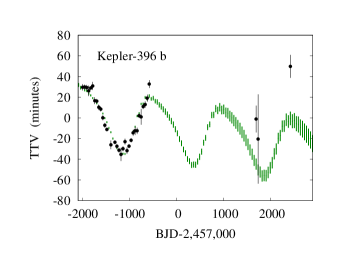
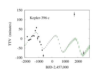
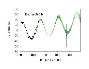
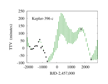
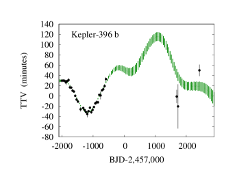
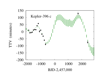
Figure 5: TTV models ($O-C$, in minutes) for Kepler-396, with the combined Kepler/TESS transit times in black and 68% confidence intervals with equal weight in the tails on simulated transit times in green. The top row corresponds to a two-planet model, the middle row includes a nontransiting planet orbiting beyond Kepler-396 c (model A), and the bottom row includes a nontransiting planet orbiting between Kepler-396 b and Kepler-396 c (model B).

KOI	$P$ (days)	$T_{0}$ (days)	$e\cos\omega$	$e\sin\omega$	$\frac{M_{p}}{M_{\star}}\frac{M_{\odot}}{M_{\oplus}}$	$\frac{M_{p}}{M_{\oplus}}$	$\frac{R_{p}}{R_{\oplus}}$	$\rho_{p}$ (g cm-3)
2672.02	42.9921 ${}^{+0.0002}_{-0.0002}$	-1316.6357 ${}^{+0.0007}_{-0.0007}$	-0.007 ${}^{+0.002}_{-0.003}$	-0.005 ${}^{+0.002}_{-0.002}$	10.1 ${}^{+1.1}_{-1.1}$	9.5 ${}^{+1.2}_{-1.1}$	3.23 ${}^{+0.50}_{-0.19}$	1.55 ${}^{+1.04}_{-0.55}$
2672.01	88.5168 ${}^{+0.0005}_{-0.0005}$	-1276.2080 ${}^{+0.0011}_{-0.0011}$	0.059 ${}^{+0.006}_{-0.006}$	0.022 ${}^{+0.004}_{-0.004}$	12.6 ${}^{+1.7}_{-1.6}$	11.8 ${}^{+1.8}_{-1.6}$	4.58 ${}^{+0.13}_{-0.12}$	0.68 ${}^{+0.12}_{-0.10}$
2672.02	42.9926 ${}^{+0.0002}_{-0.0002}$	-1316.6383 ${}^{+0.0007}_{-0.0006}$	-0.095 ${}^{+0.025}_{-0.032}$	-0.031 ${}^{+0.006}_{-0.008}$	5.92 ${}^{+2.93}_{-1.57}$	5.60 ${}^{+2.82}_{-1.51}$	3.23 ${}^{+0.50}_{-0.19}$	0.95 ${}^{+0.84}_{-0.40}$
2672.01	88.5231 ${}^{+0.0025}_{-0.0015}$	-1276.1964 ${}^{+0.0026}_{-0.0059}$	-0.035 ${}^{+0.016}_{-0.021}$	-0.067 ${}^{+0.013}_{-0.017}$	4.91 ${}^{+1.62}_{-1.18}$	4.64 ${}^{+1.53}_{-1.14}$	4.58 ${}^{+0.13}_{-0.12}$	0.27 ${}^{+0.09}_{-0.07}$
2672x	140.9352 ${}^{+0.0781}_{-0.0867}$	-1233.5344 ${}^{+8.5149}_{-1.8773}$	-0.099 ${}^{+0.043}_{-0.021}$	-0.038 ${}^{+0.123}_{-0.024}$	$<$ 6.18	$<$ 5.99	—	—
2672.02	42.9919 ${}^{+0.0002}_{-0.0002}$	-1316.6379 ${}^{+0.0006}_{-0.0006}$	-0.062 ${}^{+0.009}_{-0.010}$	0.019 ${}^{+0.005}_{-0.004}$	6.93 ${}^{+0.93}_{-0.88}$	6.54 ${}^{+0.99}_{-0.92}$	3.23 ${}^{+0.50}_{-0.19}$	1.08 ${}^{+0.74}_{-0.39}$
2672x	57.3666 ${}^{+0.0085}_{-0.0082}$	-1288.0842 ${}^{+0.1530}_{-0.1576}$	0.019 ${}^{+0.007}_{-0.007}$	-0.154 ${}^{+0.010}_{-0.011}$	0.20 ${}^{+0.03}_{-0.03}$	0.19 ${}^{+0.03}_{-0.03}$	—	—
2672.01	88.5173 ${}^{+0.0006}_{-0.0006}$	-1276.2048 ${}^{+0.0011}_{-0.0012}$	-0.021 ${}^{+0.016}_{-0.016}$	0.067 ${}^{+0.008}_{-0.008}$	5.35 ${}^{+0.58}_{-0.57}$	5.05 ${}^{+0.64}_{-0.61}$	4.58 ${}^{+0.13}_{-0.12}$	0.29 ${}^{+0.05}_{-0.04}$

Table 7: Posteriors summarized for KOI-2672 (Kepler-396) at the epoch BJD = 2,455,680, with Two Planets (Top Section), and fits to possible Three-planet Models in Lower Sections, with a Putative Nontransiting Planet named KOI-2672x in Lower Sections. Note. The columns denote the planet, orbital period, first transit after epoch given in BJD-2,457,000, e$\cos\omega$, e$\sin\omega$, dynamical mass scaled to the Earth-Sun system, mass and radius in Earth units, and bulk density in g cm^-3.

After burn-in, model fits with an additional planet beyond Kepler-396 c (model A) settled at an orbital period $\approx$140.9 days. In this case, the additional perturber interacts only with Kepler-396 c owing to the near 3:2 resonance with a TTV periodicity $\approx 770$ days, while its period ratio with Kepler-396 b is 3.3, far from any low-order resonance. By contrast, in model B, with the perturber between the known planets, TTVs with a periodicity $\approx 1027$ days are caused by the near 3:2 resonance with Kepler-396 c. In this case, the orbital periods of Kepler-396 b and the putative perturber at $\approx$57.4 days are consistent with a 4:3 mean motion resonance.

Despite these different configurations, the masses of the transiting planets in the three-planet models agree closely (see Table 7). Between the two cases here, we note that model A is preferred over model B by a significant $\Delta$BIC. The projected transit times for the two models disagree, and hence more observations could further constrain this system. Predicted transit times for the two distinct models are listed in the appendix in Table 11.

3.3.2 KOI-94, Kepler-89

Kepler-89 has four transiting planets. Weiss et al. (2013) found a strong signal in RV and measured the mass of Kepler-89 d at 106 $\pm$ 11 $M_{\oplus}$. In addition, they reported a weak detection of Kepler-89 b (10.5 $\pm$ 4.6 $M_{\oplus}$) and upper limits only on the other planets.

Masuda et al. (2013) found a lower mass for Kepler-89 d from the TTVs ($52.1^{+6.9}_{-7.1}$ $M_{\oplus}$). The TTV signals seen in Kepler-89 c and Kepler-89 d (see Figure 6) can be attributed to the $\sim$160-day periodicity from their proximity to the 2:1 resonance. Kepler-89 e has a strong TTV signal with a periodicity 0f $\sim$730 days. However, with large data gaps and missing transits in the transit timing catalog, the period, phase, and amplitude of this TTV signal are poorly constrained. In any case, the TTVs observed in Kepler-89 e are unlikely to be caused by any of the other transiting planets. It is far from any low-order resonance with other known planets; the period ratio between Kepler-89 e and its adjacent inner neighbor Kepler-89 d is 2.34.

Since these earlier studies, the stellar mass of Kepler-89 has been revised slightly upward, from 1.28 $M_{\odot}$ to 1.34 $M_{\odot}$. This revision would cause the measured mass of Kepler-89 d from RV to be 111 $M_{\oplus}$.

With a four-planet model for the TTV at KOI-94 (Kepler-89), we find a mass for KOI-94.01 (Kepler-89 d) higher than those of Masuda et al. (2013) and Battley et al. (2021). However, as shown in Table 8, the best-fit TTV model with the four transiting planets does not provide a good fit overall, with a reduced $\chi^{2}=2.48$.

We performed dynamical fits to the measured transit times with an additional planet included in the models. There are many possible solutions for an additional planet to explain the $\sim$730-day periodicity in the TTVs of Kepler-89 e, and it is beyond the purposes of this study to thoroughly explore these possibilities. Here we briefly explore two cases. In both cases, we retain the relative compactness of the Kepler-89 system, with the TTVs caused by near mean motion resonances. While there are systems of massive nontransiting planets causing TTVs near their orbital periods and confirmed with RV (e.g. Kepler-419 Almenara et al. 2018, Kepler-448 and Kepler-693, Masuda 2017), in each of these cases the nontransiting perturber is significantly more massive than Jupiter. In the case of Kepler-89, Weiss et al. (2013) estimate an upper limit on planets at a distance of $\sim 1.7$ AU (corresponding to a period $\sim$ 700 days) to be $\sim$ 0.1 $M_{\rm{Jup}}$.

In model A, we inserted an additional planet outside the 54.32-day orbital period of Kepler-89 e, with our walkers initialized over a range of periods ranging from $\approx$93 to $\approx$124 days. For the nontransiting planet, we initialized $T_{0}$ randomly between our chosen epoch and one orbital period later. In this model, the fifth planet induces TTVs in Kepler-89 e but is too distant from the inner three planets to cause variations in their transit times. Hence, while this model is expected a priori to improve the fit to the transit times of Kepler-89 e, it is unlikely to resolve the discrepancy between the RV and four-planet TTV model in measuring the mass of Kepler-89 d.

In model B, we inserted a fifth planet interior to the orbit of Kepler-89 e with walkers initialized over a wide range of periods from $\approx$31 to $\approx$41 days. This is near the 2:3 commensurability with Kepler-89 e and near the 5:3 resonance with Kepler-89 d. Hence, in model B, the putative planet may interact with both Kepler-89 d and Kepler-89 e.

We summarize the best fits found for these four- and five-planet models in Table 8.

model	n	m	$\chi^{2}$	red. $\chi^{2}$	$\Delta$BIC
4pl	277	20	636.5	2.48	0
5pl A	277	25	474.7	1.88	-133.7
5pl B	277	25	478.4	1.90	-130.0

Table 8: Summary of Models and Best-fit Solutions for Kepler-89. Note. Models listed in the first column include fits to Kepler and TESS transit times with four (4pl) or five planets (5pl), respectively. Model A (or B) refers to fits with a fifth planet initially inserted outside the orbit of Kepler-89 e (or between Kepler-89 d and e). The second and third columns list the number of data and free parameters, the fourth column lists the lowest $\chi^{2}$ found, the fifth column notes the reduced $\chi^{2}$, and the final column gives the change in BIC compared to the four-planet model.

We found that an additional planet significantly improves the TTV model and that the additional five parameters are justified, but that there is no significant difference in the likelihood of the two different five-planet models. Our posteriors are summarized in Table 9.

The TTVs plotted in Fig 6 show that an additional planet in the system improves the TTV fit for the outermost transiting planet, Kepler-89 e. Nevertheless, several outlying transit times remain, particularly for the second half of the Kepler data for Kepler-89 c.

KOI	$P$ (days)	$T_{0}$ (days)	$e\cos\omega$	$e\sin\omega$	$\frac{M_{p}}{M_{\star}}\frac{M_{\odot}}{M_{\oplus}}$	$\frac{M_{p}}{M_{\oplus}}$	$\frac{R_{p}}{R_{\oplus}}$	$\rho_{p}$ (g cm-3)
94.04	3.74316 ${}^{+0.00004}_{-0.00004}$	-1316.6922 ${}^{+0.0009}_{-0.0009}$	-0.063 ${}^{+0.038}_{-0.044}$	0.137 ${}^{+0.047}_{-0.048}$	43 ${}^{+19}_{-16}$	58 ${}^{+25}_{-21}$	1.50 ${}^{+0.07}_{-0.04}$	95 ${}^{+46}_{-36}$
94.02	10.4284 ${}^{+0.0013}_{-0.0012}$	-1309.7511 ${}^{+0.0011}_{-0.0010}$	0.033 ${}^{+0.009}_{-0.009}$	0.003 ${}^{+0.011}_{-0.010}$	7.0 ${}^{+2.0}_{-1.6}$	94 ${}^{+2.7}_{-2.2}$	3.71 ${}^{+0.08}_{-0.07}$	1.01 ${}^{+0.30}_{-0.24}$
94.01	22.3424 ${}^{+0.0004}_{-0.0004}$	-1319.2829 ${}^{+0.0001}_{-0.0001}$	0.023 ${}^{+0.022}_{-0.018}$	0.026 ${}^{+0.020}_{-0.017}$	52.2 ${}^{+9.7}_{-8.7}$	70 ${}^{+13}_{-12}$	9.98 ${}^{+0.19}_{-0.20}$	0.39 ${}^{+0.08}_{-0.07}$
94.03	54.3261 ${}^{+0.0015}_{-0.0015}$	-1299.5999 ${}^{+0.0012}_{-0.0010}$	0.024 ${}^{+0.040}_{-0.039}$	0.008 ${}^{+0.033}_{-0.022}$	13.9 ${}^{+2.5}_{-2.2}$	19 ${}^{+3}_{-3}$	6.07 ${}^{+0.12}_{-0.18}$	0.46 ${}^{+0.09}_{-0.08}$
94.04	3.74318 ${}^{+0.00002}_{-0.00002}$	-1316.6922 ${}^{+0.0009}_{-0.0009}$	-0.084 ${}^{+0.040}_{-0.045}$	0.115 ${}^{+0.037}_{-0.036}$	37 ${}^{+15}_{-12}$	50 ${}^{+19}_{-16}$	1.50 ${}^{+0.07}_{-0.04}$	81 ${}^{+36}_{-28}$
94.02	10.4254 ${}^{+0.0009}_{-0.0010}$	-1309.7536 ${}^{+0.0008}_{-0.0007}$	0.046 ${}^{+0.014}_{-0.010}$	-0.001 ${}^{+0.011}_{-0.009}$	4.2 ${}^{+1.3}_{-1.2}$	5.6 ${}^{+1.8}_{-1.6}$	3.71 ${}^{+0.08}_{-0.07}$	0.60 ${}^{+0.20}_{-0.18}$
94.01	22.3427 ${}^{+0.0003}_{-0.0003}$	-1319.2828 ${}^{+0.0001}_{-0.0001}$	0.025 ${}^{+0.012}_{-0.010}$	-0.007 ${}^{+0.014}_{-0.012}$	37 ${}^{+8}_{-8}$	49 ${}^{+11}_{-11}$	9.98 ${}^{+0.19}_{-0.20}$	0.27 ${}^{+0.06}_{-0.06}$
94.03	54.3240 ${}^{+0.0013}_{-0.0013}$	-1299.5951 ${}^{+0.0007}_{-0.0008}$	0.025 ${}^{+0.017}_{-0.018}$	-0.005 ${}^{+0.020}_{-0.019}$	19 ${}^{+4}_{-3}$	25.2 ${}^{+5.1}_{-4.2}$	6.07 ${}^{+0.12}_{-0.18}$	0.62 ${}^{+0.13}_{-0.11}$
94x	118.0 ${}^{+0.4}_{-0.6}$	-1312.3 ${}^{+8.5}_{-5.9}$	0.040 ${}^{+0.057}_{-0.087}$	-0.082 ${}^{+0.043}_{-0.039}$	7.0 ${}^{+2.6}_{-1.8}$	9.4 ${}^{+3.5}_{-2.4}$	—	—
94.04	3.74316 ${}^{+0.00004}_{-0.00005}$	-1316.6922 ${}^{+0.0009}_{-0.0009}$	-0.054 ${}^{+0.067}_{-0.068}$	0.112 ${}^{+0.054}_{-0.063}$	$<$ 65	$<$ 87	1.50 ${}^{+0.07}_{-0.04}$	$<$ 153
94.02	10.4265 ${}^{+0.0014}_{-0.0014}$	-1309.7529 ${}^{+0.0013}_{-0.0012}$	0.025 ${}^{+0.011}_{-0.007}$	0.006 ${}^{+0.012}_{-0.008}$	5.2 ${}^{+1.9}_{-1.7}$	6.9 ${}^{+2.5}_{-2.3}$	3.71 ${}^{+0.08}_{-0.07}$	0.74 ${}^{+0.27}_{-0.25}$
94.01	22.3423 ${}^{+0.0004}_{-0.0003}$	-1319.2827 ${}^{+0.0002}_{-0.0002}$	-0.011 ${}^{+0.013}_{-0.012}$	0.009 ${}^{+0.016}_{-0.013}$	43 ${}^{+10}_{-10}$	57 ${}^{+13}_{-14}$	9.98 ${}^{+0.19}_{-0.20}$	0.32 ${}^{+0.08}_{-0.08}$
94x	39.99 ${}^{+0.03}_{-0.03}$	-1307.5 ${}^{+0.9}_{-0.6}$	0.020 ${}^{+0.034}_{-0.030}$	-0.023 ${}^{+0.030}_{-0.027}$	0.53 ${}^{+0.23}_{-0.19}$	0.71 ${}^{+0.31}_{-0.25}$	—	—
94.03	54.3268 ${}^{+0.0018}_{-0.0018}$	-1299.5960 ${}^{+0.0008}_{-0.0008}$	-0.025 ${}^{+0.024}_{-0.022}$	0.000 ${}^{+0.022}_{-0.021}$	15.5 ${}^{+3.0}_{-2.7}$	20.7 ${}^{+4.0}_{-3.6}$	6.07 ${}^{+0.12}_{-0.18}$	0.51 ${}^{+0.11}_{-0.09}$

Table 9: Posteriors Summarized for Kepler-89 at the Epoch BJD = 2,455,680, with Four Planets (Top Section), and Fits to Possible Five-planet Models in Lower Sections, with a Putative Nontransiting Planet Named KOI-94x. Note. The columns denote the planet, orbital period, first transit after epoch given in BJD-2,457,000, e$\cos\omega$, e$\sin\omega$, dynamical mass scaled to the Earth-Sun system, mass and radius in Earth units, and bulk density in g cm^-3.

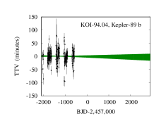
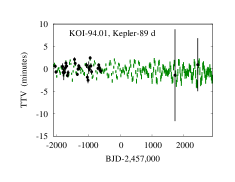
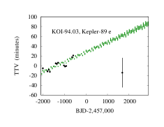
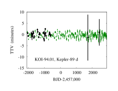
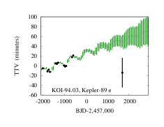
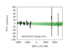
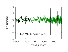
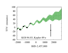
Figure 6: TTV models ($O-C$, in minutes) for KOI-94 (Kepler-89), with the combined Kepler/TESS transit times in black and 68% confidence intervals with equal weight in the tails on simulated transit times in green. The top row corresponds to a four-planet model, the middle row includes a nontransiting planet orbiting beyond Kepler-89 e (model A), and the bottom row includes a nontransiting planet orbiting between Kepler-89 d and Kepler-89 e (model B).

We find similar mass constraints on KOI-94.01 (Kepler-89 d) in both five-planet models, although the results are even more discrepant with the RV data than the four-planet model is. The mass of KOI-94.02 (Kepler-89 c) is lower in the five-planet models than the four-planet model, and the two solutions are consistent with each other.

Most of the improvement in the fit from an additional planet appears in the TTVs of Kepler-89 e, which has a $\sim$730-day periodicity that cannot be explained by near-resonant interactions with the other transiting planets. In both of our five-planet models, the additional planet induces TTVs at this periodicity and improves the fit. The measured transit times from TESS for Kepler-89 c and Kepler-89 d are consistent with prior models, although their uncertainties are too large to have an important effect on the model fits. However, none of our models closely fit the measured transit time from TESS for Kepler-89 e.

In summary, the TESS photometry does not appear to resolve the discrepancy between the TTV masses and the RV data, and while our tests of two different five-planet models improved the fit to the Kepler data, neither provided a good fit to the measured transit time of Kepler-89 e from TESS.

3.4 Other systems

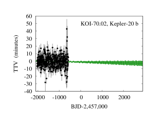
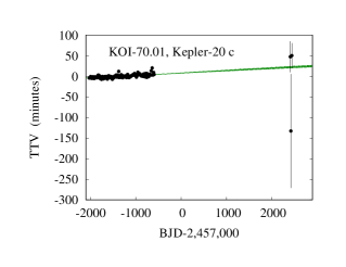
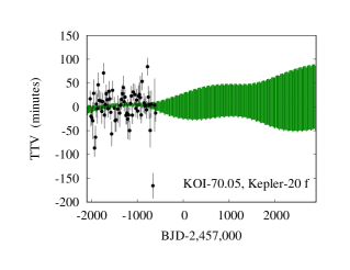
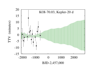
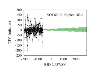
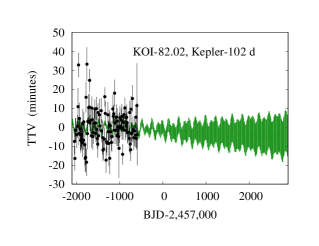
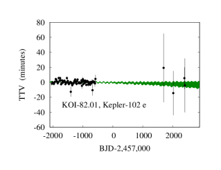
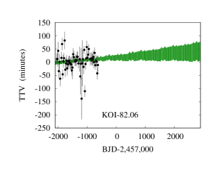
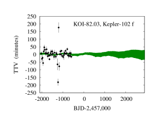
Figure 7: TTV models ($O-C$, in minutes) for planet candidates identified within each panel, with the combined Kepler /TESS transit times in black, and 68% confidence intervals with equal weight in the tails on simulated transit times in green. (Part 1 of 3.)

We list our results for the remaining systems in Table 10 and display their TTVs in Figures 7,  8 and 9.

KOI	$P$ (days)	$T_{0}$ (days)	$e\cos\omega$	$e\sin\omega$	$\frac{M_{p}}{M_{\star}}\frac{M_{\odot}}{M_{\oplus}}$	Mp (M⊕)	Rp (R⊕)	$\rho_{p}$ (g cm-3)
70.02	3.69605 ${}^{+0.00005}_{-0.00008}$	-1319.1472 ${}^{+0.0004}_{-0.0004}$	-0.012 ${}^{+0.037}_{-0.034}$	-0.013 ${}^{+0.025}_{-0.032}$	$<$ 17	$<$ 16	1.71 ${}^{+0.05}_{-0.03}$	$<$ 18
70.04	6.09844 ${}^{+0.00041}_{-0.00041}$	-1317.5396 ${}^{+0.0017}_{-0.0017}$	0.005 ${}^{+0.030}_{-0.031}$	-0.003 ${}^{+0.029}_{-0.030}$	$<$ 6.6	$<$ 6.0	0.81 ${}^{+0.04}_{-0.03}$	$<$ 68
70.01	10.85434 ${}^{+0.00018}_{-0.00015}$	-1312.0217 ${}^{+0.0003}_{-0.0003}$	-0.035 ${}^{+0.036}_{-0.030}$	0.005 ${}^{+0.027}_{-0.021}$	$<$ 36	$<$ 34	2.87 ${}^{+0.15}_{-0.07}$	$<$ 8.3
70.05	19.57800 ${}^{+0.00115}_{-0.00086}$	-1307.4195 ${}^{+0.0038}_{-0.0027}$	-0.013 ${}^{+0.029}_{-0.030}$	-0.008 ${}^{+0.024}_{-0.026}$	$<$ 6.0	$<$ 5.5	0.86 ${}^{+0.05}_{-0.03}$	$<$ 49
70.03	77.61201 ${}^{+0.00029}_{-0.00028}$	-1303.7691 ${}^{+0.0007}_{-0.0007}$	-0.029 ${}^{+0.068}_{-0.065}$	0.036 ${}^{+0.066}_{-0.086}$	$<$ 145	$<$ 133	2.49 ${}^{+0.07}_{-0.05}$	$<$ 48
82.05	5.2868 ${}^{+0.0001}_{-0.0001}$	-1317.4130 ${}^{+0.0037}_{-0.0027}$	-0.053 ${}^{+0.046}_{-0.053}$	0.076 ${}^{+0.046}_{-0.050}$	$<$ 4.2	$<$ 3.2	0.51 ${}^{+0.10}_{-0.05}$	$<$ 246
82.04	7.0713 ${}^{+0.0003}_{-0.0002}$	-1319.8768 ${}^{+0.0023}_{-0.0020}$	-0.044 ${}^{+0.040}_{-0.045}$	0.067 ${}^{+0.039}_{-0.046}$	$<$ 4.9	$<$ 3.7	0.63 ${}^{+0.18}_{-0.05}$	$<$ 401
82.02	10.3123 ${}^{+0.0008}_{-0.0005}$	-1311.0958 ${}^{+0.0014}_{-0.0013}$	-0.026 ${}^{+0.057}_{-0.062}$	0.044 ${}^{+0.041}_{-0.047}$	0.76 ${}^{+0.51}_{-0.36}$	0.59 ${}^{+0.40}_{-0.28}$	1.34 ${}^{+0.03}_{-0.12}$	1.3 ${}^{+0.9}_{-0.6}$
82.01	16.1459 ${}^{+0.0002}_{-0.0002}$	-1305.6906 ${}^{+0.0004}_{-0.0005}$	0.001 ${}^{+0.032}_{-0.036}$	0.001 ${}^{+0.029}_{-0.038}$	$<$ 5.5	$<$ 4.2	2.48 ${}^{+0.04}_{-0.21}$	$<$ 1.6
82.06	22.4108 ${}^{+0.0012}_{-0.0009}$	-1302.4960 ${}^{+0.0048}_{-0.0040}$	-0.021 ${}^{+0.043}_{-0.031}$	-0.009 ${}^{+0.033}_{-0.039}$	$<$ 0.78	$<$ 0.60	0.75 ${}^{+0.05}_{-0.05}$	$<$ 8.4
82.03	27.4546 ${}^{+0.0010}_{-0.0007}$	-1308.1785 ${}^{+0.0024}_{-0.0028}$	0.003 ${}^{+0.033}_{-0.034}$	-0.004 ${}^{+0.031}_{-0.037}$	$<$ 1.2	$<$ 0.90	0.95 ${}^{+0.11}_{-0.10}$	$<$ 6.3
137.03	3.50470 ${}^{+0.00008}_{-0.00005}$	-1318.5278 ${}^{+0.0005}_{-0.0005}$	-0.005 ${}^{+0.033}_{-0.039}$	0.018 ${}^{+0.045}_{-0.035}$	$<$ 36	$<$ 34	1.76 ${}^{+0.17}_{-0.15}$	$<$ 36
137.01	7.64149 ${}^{+0.00019}_{-0.00026}$	-1313.2815 ${}^{+0.0004}_{-0.0004}$	0.002 ${}^{+0.004}_{-0.004}$	-0.031 ${}^{+0.016}_{-0.014}$	6.4 ${}^{+3.4}_{-1.6}$	6.29 ${}^{+3.29}_{-1.59}$	4.26 ${}^{+0.08}_{-0.07}$	0.45 ${}^{+0.24}_{-0.11}$
137.02	14.85905 ${}^{+0.00062}_{-0.00026}$	-1310.7611 ${}^{+0.0006}_{-0.0003}$	-0.004 ${}^{+0.016}_{-0.016}$	-0.031 ${}^{+0.023}_{-0.029}$	8.9 ${}^{+3.0}_{-1.7}$	8.73 ${}^{+2.95}_{-1.66}$	5.16 ${}^{+0.10}_{-0.11}$	0.35 ${}^{+0.12}_{-0.07}$
244.02	6.23826 ${}^{+0.00005}_{-0.00005}$	-1315.2951 ${}^{+0.0003}_{-0.0004}$	0.020 ${}^{+0.033}_{-0.020}$	0.063 ${}^{+0.059}_{-0.037}$	$<$ 2.5	$<$ 2.6	2.78 ${}^{+0.06}_{-0.06}$	$<$ 0.66
244.01	12.72062 ${}^{+0.00005}_{-0.00005}$	-1314.2915 ${}^{+0.0001}_{-0.0001}$	0.010 ${}^{+0.042}_{-0.033}$	0.018 ${}^{+0.075}_{-0.046}$	2.4 ${}^{+2.0}_{-1.2}$	2.52 ${}^{+2.07}_{-1.22}$	5.23 ${}^{+0.10}_{-0.38}$	0.10 ${}^{+0.08}_{-0.05}$
245.03	13.36812 ${}^{+0.00075}_{-0.00074}$	-1314.5933 ${}^{+0.0074}_{-0.0073}$	0.152 ${}^{+0.052}_{-0.047}$	-0.124 ${}^{+0.022}_{-0.024}$	0.68 ${}^{+0.46}_{-0.23}$	0.52 ${}^{+0.36}_{-0.18}$	0.28 ${}^{+0.03}_{-0.02}$	133 ${}^{+118}_{-56}$
245.02	21.30001 ${}^{+0.00072}_{-0.00068}$	-1314.8005 ${}^{+0.0021}_{-0.0022}$	0.025 ${}^{+0.010}_{-0.009}$	0.005 ${}^{+0.011}_{-0.015}$	$<$ 1.6	$<$ 1.2	0.74 ${}^{+0.03}_{-0.02}$	$<$ 17
245.01	39.79212 ${}^{+0.00007}_{-0.00005}$	-1315.2820 ${}^{+0.0003}_{-0.0003}$	0.040 ${}^{+0.013}_{-0.012}$	-0.050 ${}^{+0.009}_{-0.009}$	44 ${}^{+13}_{-12}$	34 ${}^{+11}_{-9}$	1.95 ${}^{+0.05}_{-0.04}$	25 ${}^{+8}_{-7}$
282.02	8.45738 ${}^{+0.00016}_{-0.00025}$	-1317.5050 ${}^{+0.0012}_{-0.0012}$	0.027 ${}^{+0.072}_{-0.066}$	-0.027 ${}^{+0.060}_{-0.058}$	$<$ 190	$<$ 193	1.01 ${}^{+0.02}_{-0.05}$	$<$ 1036
282.01	27.50860 ${}^{+0.00176}_{-0.00065}$	-1297.1777 ${}^{+0.0019}_{-0.0010}$	0.033 ${}^{+0.027}_{-0.033}$	0.004 ${}^{+0.021}_{-0.016}$	$<$ 302	$<$ 309	2.93 ${}^{+0.18}_{-0.12}$	$<$ 73
282.03	87.52747 ${}^{+0.01002}_{-0.00568}$	-1265.6949 ${}^{+0.0104}_{-0.0045}$	0.039 ${}^{+0.103}_{-0.183}$	0.066 ${}^{+0.063}_{-0.049}$	25 ${}^{+14}_{-11}$	25 ${}^{+15}_{-11}$	1.82 ${}^{+0.15}_{-0.58}$	23 ${}^{+16}_{-11}$
377.01	19.24750 ${}^{+0.00002}_{-0.00002}$	-1309.9972 ${}^{+0.0002}_{-0.0002}$	0.055 ${}^{+0.001}_{-0.001}$	0.0123 ${}^{+0.0002}_{-0.0002}$	45.4 ${}^{+0.6}_{-0.6}$	46.5 ${}^{+2.2}_{-2.3}$	7.91 ${}^{+0.16}_{-0.16}$	0.52 ${}^{+0.04}_{-0.04}$
377.02	38.94403 ${}^{+0.00008}_{-0.00008}$	-1292.0357 ${}^{+0.0004}_{-0.0004}$	-0.0639 ${}^{+0.0001}_{-0.0001}$	0.0022 ${}^{+0.0002}_{-0.0002}$	31.3 ${}^{+0.4}_{-0.4}$	32.0 ${}^{+1.5}_{-1.6}$	8.14 ${}^{+0.18}_{-0.18}$	0.33 ${}^{+0.03}_{-0.02}$
620.01	45.15393 ${}^{+0.00036}_{-0.00038}$	-1285.4040 ${}^{+0.0006}_{-0.0006}$	-0.019 ${}^{+0.009}_{-0.010}$	-0.059 ${}^{+0.019}_{-0.022}$	2.8 ${}^{+1.4}_{-1.2}$	2.48 ${}^{+1.23}_{-1.04}$	6.62 ${}^{+0.19}_{-0.17}$	0.05 ${}^{+0.02}_{-0.02}$
620.03	85.31553 ${}^{+0.00138}_{-0.00109}$	-1274.4886 ${}^{+0.0030}_{-0.0030}$	0.024 ${}^{+0.014}_{-0.014}$	-0.048 ${}^{+0.027}_{-0.029}$	3.52 ${}^{+0.51}_{-0.51}$	3.14 ${}^{+0.50}_{-0.48}$	8.98 ${}^{+2.84}_{-2.84}$	0.02 ${}^{+0.05}_{-0.01}$
620.02	130.1827 ${}^{+0.0009}_{-0.0009}$	-1304.0693 ${}^{+0.0009}_{-0.0009}$	0.014 ${}^{+0.011}_{-0.011}$	-0.037 ${}^{+0.022}_{-0.024}$	5.83 ${}^{+1.27}_{-1.15}$	5.22 ${}^{+1.17}_{-1.07}$	9.04 ${}^{+0.25}_{-0.23}$	0.04 ${}^{+0.01}_{-0.01}$
806.03	29.35527 ${}^{+0.00043}_{-0.00042}$	-1311.7788 ${}^{+0.0026}_{-0.0027}$	-0.0079 ${}^{+0.0006}_{-0.0006}$	0.0326 ${}^{+0.0004}_{-0.0004}$	9.47 ${}^{+0.15}_{-0.15}$	8.63 ${}^{+0.42}_{-0.41}$	1.89 ${}^{+0.10}_{-0.16}$	7.1 ${}^{+1.3}_{-1.0}$
806.02	60.31922 ${}^{+0.00024}_{-0.00023}$	-1319.8839 ${}^{+0.0003}_{-0.0003}$	0.0087 ${}^{+0.0006}_{-0.0006}$	-0.0084 ${}^{+0.0005}_{-0.0005}$	546 ${}^{+5}_{-5}$	498 ${}^{+24}_{-23}$	12.03 ${}^{+0.41}_{-0.40}$	1.57 ${}^{+0.19}_{-0.16}$
806.01	143.4992 ${}^{+0.0036}_{-0.0037}$	-1296.7204 ${}^{+0.0011}_{-0.0011}$	-0.0262 ${}^{+0.0013}_{-0.0013}$	-0.0078 ${}^{+0.0013}_{-0.0013}$	20.1 ${}^{+1.4}_{-1.4}$	18.3 ${}^{+1.5}_{-1.5}$	8.79 ${}^{+0.49}_{-0.31}$	0.15 ${}^{+0.03}_{-0.02}$
1353.02	34.54304 ${}^{+0.00101}_{-0.00096}$	-1308.8883 ${}^{+0.0024}_{-0.0022}$	-0.003 ${}^{+0.030}_{-0.027}$	-0.061 ${}^{+0.036}_{-0.040}$	$<$ 13.5	$<$ 14.2	2.41 ${}^{+0.41}_{-0.34}$	$<$ 8.5
K289d	65.95930 ${}^{+0.00145}_{-0.00168}$	-1298.0481 ${}^{+0.0028}_{-0.0028}$	-0.003 ${}^{+0.001}_{-0.001}$	-0.028 ${}^{+0.007}_{-0.009}$	2.89 ${}^{+0.50}_{-0.44}$	3.04 ${}^{+0.55}_{-0.47}$	2.65 ${}^{+1.08}_{-0.19}$	0.9 ${}^{+3.4}_{-0.6}$
1353.01	125.8697 ${}^{+0.0007}_{-0.0005}$	-1301.0103 ${}^{+0.0004}_{-0.0003}$	0.009 ${}^{+0.005}_{-0.005}$	-0.002 ${}^{+0.008}_{-0.011}$	116 ${}^{+11}_{-11}$	122 ${}^{+12}_{-13}$	11.14 ${}^{+0.23}_{-0.23}$	0.48 ${}^{+0.06}_{-0.06}$
1783.01	134.4629 ${}^{+0.0034}_{-0.0035}$	-1190.8662 ${}^{+0.0039}_{-0.0038}$	0.007 ${}^{+0.007}_{-0.005}$	-0.047 ${}^{+0.014}_{-0.016}$	78.9 ${}^{+16.2}_{-13.2}$	89 ${}^{+19}_{-16}$	9.03 ${}^{+0.23}_{-0.24}$	0.67 ${}^{+0.16}_{-0.13}$
1783.02	284.2162 ${}^{+0.0280}_{-0.0215}$	-1113.8267 ${}^{+0.0292}_{-0.0217}$	0.018 ${}^{+0.015}_{-0.014}$	-0.018 ${}^{+0.034}_{-0.029}$	16.3 ${}^{+4.8}_{-3.9}$	18.5 ${}^{+5.5}_{-4.4}$	5.46 ${}^{+0.51}_{-0.30}$	0.63 ${}^{+0.31}_{-0.20}$

Table 10: Posteriors Summarized for Orbital Parameters, Dynamical Masses, and Bulk Planet Properties at the Epoch BJD=2,455,680 (Noted as BJD$-$2,457,000), With Measured Times from TESS in Addition to Kepler Light-curve Transit Times (Rowe & Thompson, 2015) (with Some Exceptions Noted in §3.1). Note. The columns denote orbital period in days, the first transit time after epoch, eccentricity vector components, dynamical mass scaled to the Earth-Sun system, planetary masses, radii and bulk densities. Summary statistics of the posteriors include the median and 68.3% confidence intervals with equal weight in the tails. Upper limits list the 97.7th percentile of the posterior distribution. Note Kepler-289 d (PH3 c, orbiting KOI-1353) does not have a KOI number.

KOI-70 (Kepler-20) has five transiting planets. This system was selected because of a near 3:1 resonance between KOI-70.01 and KOI-70.02, with an expected periodicity $\approx$ 171 days, although no TTVs were reported by Holczer et al. (2016). Buchhave et al. (2016) discovered a nontransiting planet in RV with an orbital period of 34.94 days. This additional planet, while between Kepler-20 c and Kepler-20 d, is far from any low-order resonance with other planets and is unlikely to cause detectable TTV. Indeed, no TTVs were found in this system by Buchhave et al. (2016), and we exclude this additional planet from our analysis.

The two relatively precise measured transit times from TESS are consistent with a linear ephemeris for KOI-70.01, and the third transit time is too uncertain to have an effect on the models. The outer pair at KOI-70 are close to the 4:1 commensurability, with an expected TTV periodicity of $\approx$2171 days. This can be seen in the projected TTV of both planets, leading to the prospect of more meaningful upper limits on their masses with future data, although both planets are too small to be detected in TESS light curves.

KOI-82 (Kepler-102) has six known planet candidates. The overall configuration is more compact than Kepler-11 (Lissauer et al., 2011b), requiring low masses for stability. However, there are few adjacent pairs near resonance, making the TTV signals weak. Our upper limits in mass for most of the planets at Kepler-102 are uninformative, given the planetary radii. However, our results for KOI-82.02 (Kepler-102 d) and KOI-82.01 (Kepler-102 e), as well as revised planet radius measurements, provide evidence for lower bulk densities than found from the weak RV signal observed by Marcy et al. (2014).

KOI-137 (Kepler-18) has three transiting planets with planetary masses measured by a combined RV and TTV data set (Cochran et al., 2011). Kepler-18 b has no evidence of interaction with Kepler-18 c, and its mass is poorly constrained from the TTV alone. Kepler-18 c and Kepler-18 d have anticorrelated TTVs with a periodicity $\sim$270 days. The mass constraints following TESS agree closely with the results of Jontof-Hutter et al. (2021).

KOI-244 (Kepler-25) has two planets with strongly detected anticorrelated TTVs (Lithwick et al., 2012). The TTV periodicity at $\sim$325 days is well sampled by the Kepler data set. The masses following TESS transit times are in close agreement with the masses following dynamical fits with Kepler-only transit times (Jontof-Hutter et al., 2021) and lower than those found via RV (Marcy et al., 2014). Hadden & Lithwick (2017) found that the TTV posteriors are sensitive to priors in eccentricity, and there is closer agreement between the RV and TTV masses with a low-eccentricity prior.

Jontof-Hutter et al. (2021) projected the transit times of Kepler-18 and Kepler-25, and found very little divergence in the decades following the Kepler mission, suggesting that TESS data would not significantly improve the TTV model. Our results confirm that expectation and agree closely with previous mass estimates. For both of these systems, our results are also closely consistent with Battley et al. (2021).

KOI-245 (Kepler-37) did not have a detection of TTVs reported in Holczer et al. (2016). However, there is an expected TTV periodicity of $\sim$300 days, due to the near 2:1 resonance of Kepler-37 c and Kepler-37 d. There is a fourth candidate (KOI-245.04), with a period of 51.22 days, that is dispositioned in the DR25 Supplement as a false positive. It was earlier identified in the Q6 catalog (Batalha et al., 2013) and appears in subsequent Kepler catalogs (Burke et al. 2014; Mullally et al. 2015). Mazeh et al. (2013) published a comprehensive catalog of measured transit times following 12 quarters of Kepler light curves and included KOI-245.04, although no significant TTV signals were detected in the system. The candidate was listed as “confirmed” in the Q16 catalog of Mullally et al. (2015), possibly based on a 1$\sigma$ detection of near-resonant TTVs by Hadden & Lithwick (2014), although only its inner neighbor KOI-245.01 has mass constraints derived from the TTV. Given the small size of the putative KOI-245.04 (0.37 $R_{\oplus}$, Burke et al. 2014), and the near 5:4 resonant period with KOI-245.01, we estimate the amplitude of TTVs in KOI-245.01 potentially caused by KOI-245.04 to be of order $\sim$10 s, which would be undetectable. Hence, we excluded KOI-245.04 from our dynamical fits. In agreement with Hadden & Lithwick (2014), we find the bulk density of KOI-245.01 (Kepler-37 d) to be unphysically high. One possible explanation for the high bulk density inference is significant dilution in the Kepler light curves causing the planet radii to be underestimated. This appears unlikely; according to the ExoFOP Kepler page for KOI-245, the nearest stars in the field are 2 mag fainter. Marcy et al. (2014) reported RV data on KOI-245, and there were no detections, although the upper limit they found for the mass of KOI-245.01 (Kepler-37 d), 12.2 $M_{\oplus}$, is lower than what we find via transit timing. As noted by Hadden & Lithwick (2014) the high dynamical mass from TTV of KOI-245.01 (Kepler-37 d) given the small radius could be caused by orbital eccentricities outside of our prior.

Holczer et al. (2016) detected TTVs at KOI-282.01 (Kepler-132 c) with a periodicity of $\approx$462 days. These can be attributed to the near 3:1 commensurability with its outer neighbor. A similar period ratio exists between KOI-282.01 and its inner neighbor KOI-282.02 (Kepler-130 b), although that pair is farther from resonance, has a shorter TTV period, and has a lower TTV amplitude. The inner two planets have uninformative upper limits only, while the outer planet appears to be weakly detected at the 2$\sigma$ level. The inferred density is significantly higher than other well-characterized exoplanets. As with KOI-245, we attribute this to either eccentricities that are excluded by our prior, in which a lower mass could cause the TTVs, or an underestimate of the planet radius due to dilution. The latter is unlikely since all the identified nearby stars for this target on ExoFOP Kepler are several magnitudes fainter. The single transit detected in the TESS data does little to further constrain the planetary masses.

KOI-377 (Kepler-9) has two sub-Saturn planets that have strongly detected TTVs and a super-Earth that is dynamically isolated from the interacting pair. We included only the large planets, KOI-377.01 (Kepler-9 b) and KOI-377.02 (Kepler-9 c), in our dynamical models. We did not detect the transits of Kepler-9 in Sector 14 despite the expectation of an S/N $>$9 in the absence of correlated noise for both Kepler-9 b and Kepler-9 c. This may be due to stray-light contamination in S14/S15 (e.g. Dalba et al. 2020). For Sectors 40 and 41, we detected transits in the long-cadence data for Kepler-9. Our mass measurements agree closely with Freudenthal et al. (2018).

KOI-620 (Kepler-51) has three planets characterized from strong TTV signals (Masuda, 2014). All three have extremely low bulk densities, although the size of KOI-620.03 (Kepler-51 c) is poorly constrained owing to an impact parameter above unity. Nevertheless, a minimum size for Kepler-51 c implies a very low upper limit in density, like its neighbors. The detected TESS transit times have large uncertainties and do little to further constrain the planetary masses, as found by Battley et al. (2021).

KOI-806 (Kepler-30) has high-amplitude TTVs, with an amplitude of 1 day at the innermost planet KOI-806.03, (Kepler-30 b). The TTVs were initial modeled by Sanchis-Ojeda et al. (2012), before a complete TTV period had been observed. Studies from Wu et al. (2018), Panichi et al. (2018), and Jontof-Hutter et al. (2021) refined the TTV model after the Kepler mission. Our results agree with these studies. Despite the large TTVs in this system, the TESS measurements do not significantly improve the mass posteriors. Both KOI-806.03 (Kepler-30 c) and KOI-806.02 (Kepler-30 d) have low S/N in the TESS light curves and large transit timing uncertainties.

KOI-1353 (Kepler-289) has three planets with strongly detected TTVs. We adopted the transit times and measured planet size for Kepler-289 d of Schmitt et al. (2014), with additional transit times for the other planets from Jontof-Hutter et al. (2021). The additional transit time during the TESS mission is consistent with the projected transit times following the Kepler mission. The measured masses are in close agreement with the results following Kepler data only of Jontof-Hutter et al. (2021).

For KOI-1783 (Kepler-1662), our results are closely consistent with the corresponding models of Vissapragada et al. (2020). In that study, a single ground-based observation of KOI-1783.01 supplemented the Kepler dataset. Here we combined all three datasets.

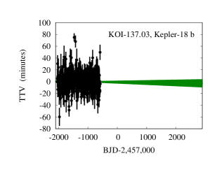
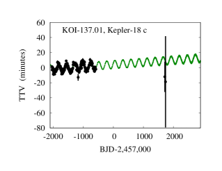
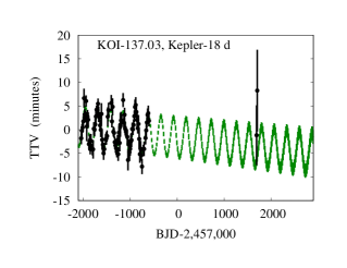
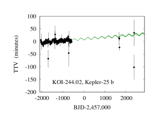
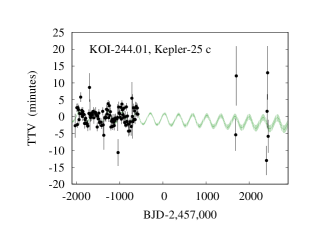
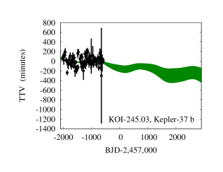
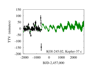
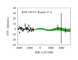
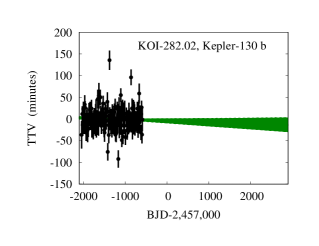
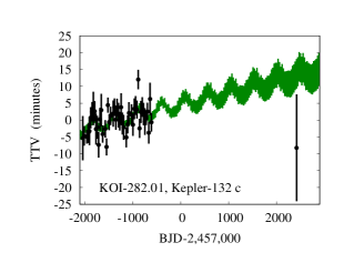
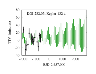
Figure 8: TTV models ($O-C$, in minutes) for planet candidates identified within each panel, with the combined Kepler /TESS transit times in black, and 68% confidence intervals with equal weight in the tails on simulated transit times in green. (Part 2 of 3.)

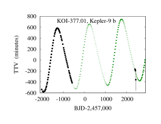
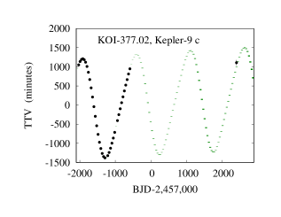
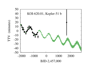
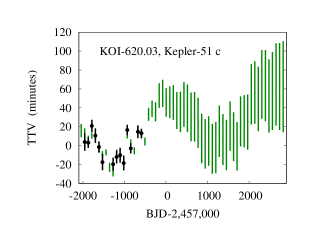
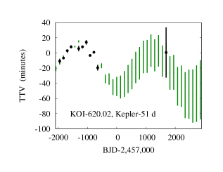
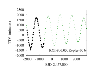
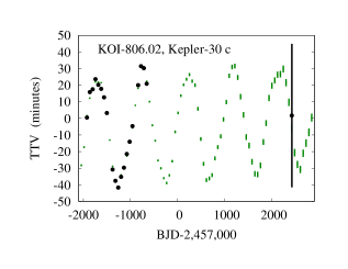
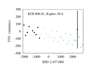
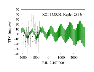
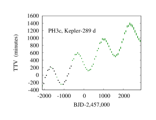
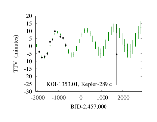
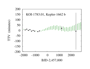
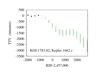
Figure 9: TTV models ($O-C$, in minutes) for planet candidates identified within each panel, with the combined Kepler /TESS transit times in black, and 68% confidence intervals with equal weight in the tails on simulated transit times in green. (Part 3 of 3.)

4 Discussion and Conclusions

For several systems, we have detected transits in TESS  data, at a significantly lower S/N than in Kepler data, with PLD. In all cases, the Kepler data are more precise and there are more measurements than in the TESS data set. Hence, the dynamical constraints we have found here are mostly driven by the Kepler data. Nevertheless, we find strong evidence of an additional perturber at KOI-2672 (Kepler-396). For two very different configurations involving an additional planet, we find closely consistent masses for the two transiting planets, results that are inconsistent with the posteriors for a two-planet model for the system. The transits detected by TESS at this system, alongside the Kepler data, are a significant improvement over the Kepler data alone for the purposes of TTV modeling. If the apparent robustness of the mass measurements of the transiting planets to different configurations with a nontransiting perturber persists with future data and additional modeling, we note that KOI-2672.01 (Kepler-396 c) has a very low density. Its orbital period and low density place it in a similar regime to the lowest density planets characterized via TTVs (e.g. Kepler-51 (Masuda 2014; Libby-Roberts et al. 2020), Kepler-79 d Jontof-Hutter et al. 2014; Chachan et al. 2020), but with a brighter host.

With several transits of KOI-94 (Kepler-89) observed by TESS  we found the one transit of KOI-94.03 (Kepler-89 e) inconsistent at 2$\sigma$ with projections from a range of TTV models that we explored here, with the four known planets, as well as with an additional planet. While the additional planet improved the model fits substantially, we did not find solutions that persisted between different five-planet models, nor did we find solutions that were consistent with the strong detection of KOI-94.01 (Kepler-89 d) in RV.

The choice to apply PLD to TESS photometry borrows from extensive experience with the noise properties of photometry taken by the Spitzer Space Telescope (e.g., Ingalls et al., 2012; Deming et al., 2015). The large pixels in the TESS spacecraft’s detectors result in undersampled PSFs for relatively faint stars. This allows any variation in pixel sensitivity, coupled with random pointing jitter and systematic drift of the spacecraft, to produce time-correlated noise that obscures astrophysical signals. The Kepler systems analyzed here are among the faintest stars for which TESS can achieve a reasonable photometric precision, making them optimal test cases for the application of PLD. Although in many cases our analysis yielded nondetections, in many others PLD enabled low S/N detections of transits that would have otherwise been hidden in the noise. This powerful and simple tool thereby expands the discovery space beyond the demographic of bright stars for which the TESS mission is optimized. Here, we have shown the benefits of this technique for the sample of Kepler planets exhibiting TTVs. Beyond these planets, though, the application of PLD to extract transits from noisy TESS data has several useful applications. Staying with Kepler, the longest-period transiting systems only exhibit a few transits (e.g., Kipping et al., 2016; Dalba et al., 2021), precluding robust TTV analyses. If the TESS extended mission continues, transits of these planets will occasionally occur during TESS observations. These will identify (or rule out) the presence of TTVs and eventually enable new dynamical investigations (e.g., Dalba & Tamburo, 2019). The benefits of PLD extend to planets discovered by TESS as well. Transits of those with orbital periods greater than the observational baseline will not show the periodicity that is usually necessary to confidently claim a planet candidate detection (Díaz et al. 2020; Dalba et al. 2022). For faint stars and/or shallow transits (i.e., small planets), these planets may go undetected or at least not validated. In these cases, PLD will enable careful searches for additional transit signals that will fill in the parameter space of planet discoveries made by the TESS mission.

Despite different host star selection functions, the Kepler and TESS missions can be highly complementary. With PLD, we have unlocked TESS’s ability to detect transits in noisy data and refined the properties of some of Kepler’s most interesting planetary systems.

We thank an anonymous referee for comments that improved this paper. D.J.-H. acknowledges grant No. 80NSSC20K1008 from the TESS GI program. P.D. is supported by a National Science Foundation (NSF) Astronomy and Astrophysics Postdoctoral Fellowship under award AST-1903811. This paper includes data collected with the TESS mission, obtained from the MAST data archive at the Space Telescope Science Institute (STScI). Funding for the TESS mission is provided by the NASA Explorer Program. STScI is operated by the Association of Universities for Research in Astronomy, Inc., under NASA contract NAS 5–26555.

This work made use of tpfplotter by J. Lillo-Box (publicly available in www.github.com/jlillo/tpfplotter), which also made use of the Python packages astropy, lightkurve, matplotlib, and numpy.

Appendix: Projected Transit Times for (KOI-2672) Kepler-396.

We list projected transit times and uncertainties for Kepler-396 b and c in Table 11.

2638.8191 $\pm$ 0.0066	3498.6522 $\pm$ 0.0067	4358.5536 $\pm$ 0.0093	5218.4140 $\pm$ 0.0096	6078.2823 $\pm$ 0.0124	6938.1826 $\pm$ 0.0141
2681.8124 $\pm$ 0.0066	3541.6482 $\pm$ 0.0066	4401.5431 $\pm$ 0.0094	5261.4116 $\pm$ 0.0097	6121.2726 $\pm$ 0.0124	6981.1784 $\pm$ 0.0144
2724.8033 $\pm$ 0.0067	3584.6441 $\pm$ 0.0065	4444.5326 $\pm$ 0.0094	5304.4087 $\pm$ 0.0099	6164.2635 $\pm$ 0.0125	7024.1760 $\pm$ 0.0148
2767.7946 $\pm$ 0.0066	3627.6407 $\pm$ 0.0065	4487.5224 $\pm$ 0.0095	5347.4073 $\pm$ 0.0103	6207.2549 $\pm$ 0.0126	7067.1702 $\pm$ 0.0150
2810.7848 $\pm$ 0.0067	3670.6376 $\pm$ 0.0065	4530.5119 $\pm$ 0.0095	5390.4039 $\pm$ 0.0105	6250.2468 $\pm$ 0.0126	7110.1659 $\pm$ 0.0152
2853.7747 $\pm$ 0.0066	3713.6345 $\pm$ 0.0066	4573.5020 $\pm$ 0.0095	5433.4024 $\pm$ 0.0110	6293.2394 $\pm$ 0.0126	7153.1584 $\pm$ 0.0153
2896.7643 $\pm$ 0.0067	3756.6321 $\pm$ 0.0067	4616.4922 $\pm$ 0.0096	5476.3983 $\pm$ 0.0113	6336.2328 $\pm$ 0.0127	7196.1518 $\pm$ 0.0154
2939.7539 $\pm$ 0.0067	3799.6294 $\pm$ 0.0069	4659.4832 $\pm$ 0.0096	5519.3957 $\pm$ 0.0116	6379.2267 $\pm$ 0.0127	7239.1428 $\pm$ 0.0154
2982.7434 $\pm$ 0.0067	3842.6277 $\pm$ 0.0072	4702.4745 $\pm$ 0.0096	5562.3899 $\pm$ 0.0118	6422.2210 $\pm$ 0.0126	7282.1341 $\pm$ 0.0154
3025.7330 $\pm$ 0.0067	3885.6244 $\pm$ 0.0075	4745.4665 $\pm$ 0.0096	5605.3855 $\pm$ 0.0120	6465.2163 $\pm$ 0.0127	7325.1244 $\pm$ 0.0155
3068.7231 $\pm$ 0.0067	3928.6229 $\pm$ 0.0080	4788.4594 $\pm$ 0.0097	5648.3780 $\pm$ 0.0121	6508.2114 $\pm$ 0.0126	7368.1144 $\pm$ 0.0155
3111.7133 $\pm$ 0.0067	3971.6185 $\pm$ 0.0082	4831.4525 $\pm$ 0.0097	5691.3713 $\pm$ 0.0121	6551.2075 $\pm$ 0.0126	7411.1040 $\pm$ 0.0156
3154.7042 $\pm$ 0.0067	4014.6160 $\pm$ 0.0086	4874.4466 $\pm$ 0.0097	5734.3622 $\pm$ 0.0121	6594.2035 $\pm$ 0.0125	7454.0937 $\pm$ 0.0156
3197.6954 $\pm$ 0.0067	4057.6101 $\pm$ 0.0088	4917.4410 $\pm$ 0.0097	5777.3537 $\pm$ 0.0121	6637.2002 $\pm$ 0.0125	7497.0833 $\pm$ 0.0157
3240.6876 $\pm$ 0.0068	4100.6056 $\pm$ 0.0090	4960.4361 $\pm$ 0.0097	5820.3437 $\pm$ 0.0122	6680.1970 $\pm$ 0.0125	7540.0730 $\pm$ 0.0157
3283.6802 $\pm$ 0.0068	4143.5980 $\pm$ 0.0091	5003.4313 $\pm$ 0.0096	5863.3337 $\pm$ 0.0121	6723.1940 $\pm$ 0.0126	7583.0632 $\pm$ 0.0158
3326.6734 $\pm$ 0.0068	4186.5911 $\pm$ 0.0092	5046.4274 $\pm$ 0.0096	5906.3235 $\pm$ 0.0123	6766.1919 $\pm$ 0.0128	7626.0534 $\pm$ 0.0159
3369.6676 $\pm$ 0.0068	4229.5822 $\pm$ 0.0093	5089.4234 $\pm$ 0.0095	5949.3129 $\pm$ 0.0122	6809.1889 $\pm$ 0.0130	7669.0444 $\pm$ 0.0159
3412.6618 $\pm$ 0.0067	4272.5735 $\pm$ 0.0093	5132.4201 $\pm$ 0.0095	5992.3026 $\pm$ 0.0123	6852.1873 $\pm$ 0.0133	7712.0356 $\pm$ 0.0159
3455.6570 $\pm$ 0.0067	4315.5634 $\pm$ 0.0093	5175.4168 $\pm$ 0.0095	6035.2923 $\pm$ 0.0124	6895.1842 $\pm$ 0.0137	7755.0278 $\pm$ 0.0160
2618.3110 $\pm$ 0.0154	3503.5568 $\pm$ 0.0930	4388.6804 $\pm$ 0.0922	5273.7746 $\pm$ 0.0737	6158.9297 $\pm$ 0.1586	7043.9941 $\pm$ 0.2790
2706.8330 $\pm$ 0.0221	3592.0599 $\pm$ 0.0945	4477.2046 $\pm$ 0.0939	5362.2726 $\pm$ 0.0723	6247.4458 $\pm$ 0.1701	7132.5141 $\pm$ 0.2927
2795.3549 $\pm$ 0.0327	3680.5607 $\pm$ 0.0947	4565.7288 $\pm$ 0.0948	5450.7678 $\pm$ 0.0750	6335.9734 $\pm$ 0.1819	7221.0397 $\pm$ 0.3078
2883.8846 $\pm$ 0.0447	3769.0571 $\pm$ 0.0966	4654.2630 $\pm$ 0.0856	5539.2667 $\pm$ 0.0799	6424.4880 $\pm$ 0.1951	7309.5599 $\pm$ 0.3199
2972.4171 $\pm$ 0.0555	3857.5549 $\pm$ 0.0986	4742.7859 $\pm$ 0.0799	5627.7837 $\pm$ 0.0911	6512.9948 $\pm$ 0.2091	7398.0872 $\pm$ 0.3310
3060.9444 $\pm$ 0.0679	3946.0744 $\pm$ 0.0913	4831.3012 $\pm$ 0.0758	5716.3039 $\pm$ 0.1017	6601.4898 $\pm$ 0.2220	7486.6160 $\pm$ 0.3380
3149.4678 $\pm$ 0.0789	4034.5913 $\pm$ 0.0901	4919.8064 $\pm$ 0.0755	5804.8281 $\pm$ 0.1129	6689.9860 $\pm$ 0.2344	7575.1392 $\pm$ 0.3447
3238.0094 $\pm$ 0.0797	4123.1132 $\pm$ 0.0923	5008.3058 $\pm$ 0.0734	5893.3507 $\pm$ 0.1247	6778.4835 $\pm$ 0.2448	7663.6595 $\pm$ 0.3512
3326.5359 $\pm$ 0.0841	4211.6287 $\pm$ 0.0923	5096.7993 $\pm$ 0.0722	5981.8774 $\pm$ 0.1369	6866.9775 $\pm$ 0.2560	7752.1916 $\pm$ 0.3548
3415.0538 $\pm$ 0.0893	4300.1534 $\pm$ 0.0920	5185.2862 $\pm$ 0.0726	6070.4075 $\pm$ 0.1472	6955.4738 $\pm$ 0.2677	7840.7109 $\pm$ 0.3603
2638.7853 $\pm$ 0.0071	3498.6611 $\pm$ 0.0253	4358.7198 $\pm$ 0.0630	5218.7414 $\pm$ 0.1088	6078.6147 $\pm$ 0.2510	6938.4049 $\pm$ 0.4725
2681.7773 $\pm$ 0.0073	3541.6617 $\pm$ 0.0269	4401.7200 $\pm$ 0.0651	5261.7443 $\pm$ 0.1114	6121.6008 $\pm$ 0.2651	6981.4006 $\pm$ 0.4903
2724.7685 $\pm$ 0.0076	3584.6642 $\pm$ 0.0286	4444.7203 $\pm$ 0.0671	5304.7456 $\pm$ 0.1141	6164.5858 $\pm$ 0.2797	7024.3974 $\pm$ 0.5097
2767.7603 $\pm$ 0.0080	3627.6665 $\pm$ 0.0302	4487.7197 $\pm$ 0.0692	5347.7476 $\pm$ 0.1166	6207.5718 $\pm$ 0.2945	7067.3940 $\pm$ 0.5307
2810.7512 $\pm$ 0.0084	3670.6704 $\pm$ 0.0319	4530.7196 $\pm$ 0.0713	5390.7466 $\pm$ 0.1185	6250.5573 $\pm$ 0.3097	7110.3912 $\pm$ 0.5533
2853.7421 $\pm$ 0.0087	3713.6728 $\pm$ 0.0337	4573.7188 $\pm$ 0.0733	5433.7468 $\pm$ 0.1205	6293.5439 $\pm$ 0.3193	7153.3872 $\pm$ 0.5773
2896.7326 $\pm$ 0.0092	3756.6771 $\pm$ 0.0355	4616.7187 $\pm$ 0.0754	5476.7459 $\pm$ 0.1215	6336.5302 $\pm$ 0.3266	7196.3842 $\pm$ 0.6024
2939.7240 $\pm$ 0.0098	3799.6804 $\pm$ 0.0372	4659.7179 $\pm$ 0.0775	5519.7449 $\pm$ 0.1232	6379.5176 $\pm$ 0.3352	7239.3809 $\pm$ 0.6284
2982.7147 $\pm$ 0.0105	3842.6853 $\pm$ 0.0391	4702.7181 $\pm$ 0.0796	5562.7398 $\pm$ 0.1256	6422.5054 $\pm$ 0.3438	7282.3778 $\pm$ 0.6555
3025.7060 $\pm$ 0.0111	3885.6886 $\pm$ 0.0410	4745.7180 $\pm$ 0.0818	5605.7352 $\pm$ 0.1300	6465.4938 $\pm$ 0.3527	7325.3736 $\pm$ 0.6833
3068.6972 $\pm$ 0.0120	3928.6931 $\pm$ 0.0429	4788.7189 $\pm$ 0.0840	5648.7293 $\pm$ 0.1362	6508.4829 $\pm$ 0.3617	7368.3703 $\pm$ 0.7120
3111.6901 $\pm$ 0.0130	3971.6967 $\pm$ 0.0448	4831.7197 $\pm$ 0.0862	5691.7229 $\pm$ 0.1439	6551.4719 $\pm$ 0.3708	7411.3673 $\pm$ 0.7415
3154.6827 $\pm$ 0.0140	4014.7011 $\pm$ 0.0468	4874.7213 $\pm$ 0.0886	5734.7134 $\pm$ 0.1526	6594.4624 $\pm$ 0.3801	7454.3654 $\pm$ 0.7720
3197.6765 $\pm$ 0.0151	4057.7044 $\pm$ 0.0487	4917.7233 $\pm$ 0.0909	5777.7040 $\pm$ 0.1625	6637.4518 $\pm$ 0.3897	7497.3624 $\pm$ 0.8037
3240.6707 $\pm$ 0.0163	4100.7080 $\pm$ 0.0508	4960.7257 $\pm$ 0.0934	5820.6935 $\pm$ 0.1734	6680.4430 $\pm$ 0.3993	7540.3609 $\pm$ 0.8361
3283.6671 $\pm$ 0.0177	4143.7107 $\pm$ 0.0528	5003.7286 $\pm$ 0.0959	5863.6826 $\pm$ 0.1850	6723.4339 $\pm$ 0.4092	7583.3596 $\pm$ 0.8688
3326.6637 $\pm$ 0.0191	4186.7137 $\pm$ 0.0548	5046.7308 $\pm$ 0.0984	5906.6696 $\pm$ 0.1973	6766.4264 $\pm$ 0.4196	7626.3596 $\pm$ 0.9025
3369.6613 $\pm$ 0.0206	4229.7157 $\pm$ 0.0569	5089.7343 $\pm$ 0.1010	5949.6569 $\pm$ 0.2101	6809.4174 $\pm$ 0.4304	7669.3590 $\pm$ 0.9383
3412.6600 $\pm$ 0.0221	4272.7176 $\pm$ 0.0589	5132.7367 $\pm$ 0.1036	5992.6431 $\pm$ 0.2234	6852.4121 $\pm$ 0.4423	7712.3604 $\pm$ 0.9751
3455.6600 $\pm$ 0.0237	4315.7186 $\pm$ 0.0610	5175.7402 $\pm$ 0.1063	6035.6296 $\pm$ 0.2371	6895.4080 $\pm$ 0.4564	7755.3622 $\pm$ 1.0133
2618.2716 $\pm$ 0.0126	3503.3184 $\pm$ 0.0438	4388.2456 $\pm$ 0.1261	5273.2409 $\pm$ 0.1844	6158.3415 $\pm$ 0.2330	7043.3611 $\pm$ 0.2725
2706.7752 $\pm$ 0.0154	3591.8029 $\pm$ 0.0515	4476.7559 $\pm$ 0.1325	5361.7370 $\pm$ 0.1884	6246.8475 $\pm$ 0.2371	7131.8698 $\pm$ 0.2774
2795.2828 $\pm$ 0.0183	3680.2889 $\pm$ 0.0594	4565.2671 $\pm$ 0.1387	5450.2369 $\pm$ 0.1930	6335.3491 $\pm$ 0.2413	7220.3814 $\pm$ 0.2821
2883.7937 $\pm$ 0.0211	3768.7756 $\pm$ 0.0676	4653.7776 $\pm$ 0.1448	5538.7398 $\pm$ 0.1979	6423.8542 $\pm$ 0.2445	7308.8966 $\pm$ 0.2868
2972.3067 $\pm$ 0.0239	3857.2642 $\pm$ 0.0761	4742.2849 $\pm$ 0.1507	5627.2461 $\pm$ 0.2031	6512.3543 $\pm$ 0.2481	7397.4119 $\pm$ 0.2910
3060.8198 $\pm$ 0.0267	3945.7551 $\pm$ 0.0847	4830.7874 $\pm$ 0.1566	5715.7563 $\pm$ 0.2084	6600.8539 $\pm$ 0.2514	7485.9296 $\pm$ 0.2953
3149.3306 $\pm$ 0.0293	4034.2487 $\pm$ 0.0934	4919.2843 $\pm$ 0.1625	5804.2701 $\pm$ 0.2137	6689.3524 $\pm$ 0.2552	7574.4523 $\pm$ 0.3013
3237.8376 $\pm$ 0.0320	4122.7450 $\pm$ 0.1021	5007.7759 $\pm$ 0.1684	5892.7870 $\pm$ 0.2189	6777.8517 $\pm$ 0.2592	7662.9742 $\pm$ 0.3071
3326.3372 $\pm$ 0.0343	4211.2450 $\pm$ 0.1109	5096.2618 $\pm$ 0.1744	5981.3061 $\pm$ 0.2240	6866.3526 $\pm$ 0.2634	7751.4948 $\pm$ 0.3127
3414.8314 $\pm$ 0.0366	4299.7436 $\pm$ 0.1185	5184.7463 $\pm$ 0.1807	6069.8244 $\pm$ 0.2286	6954.8555 $\pm$ 0.2679	7840.0111 $\pm$ 0.3183

Table 11: Predicted transit timing posteriors (BJD-2,457,000) for KOI-2672.02 (Kepler-396 b) and KOI-2672.01 (Kepler-396 c) for two possible three-planet models. The upper (lower) two panels correspond to a model with a non-transiting planet orbiting near 141 (57) days. (See Section 3.1 for more detail.)

References

- Agol & Deck (2016) Agol, E., & Deck, K. 2016, ApJ, 818, 177, doi: 10.3847/0004-637X/818/2/177
- Agol et al. (2005) Agol, E., Steffen, J., Sari, R., & Clarkson, W. 2005, MNRAS, 359, 567, doi: 10.1111/j.1365-2966.2005.08922.x
- Aller et al. (2020) Aller, A., Lillo-Box, J., Jones, D., Miranda, L. F., & Barceló Forteza, S. 2020, A&A, 635, A128, doi: 10.1051/0004-6361/201937118
- Almenara et al. (2018) Almenara, J. M., Díaz, R. F., Hébrard, G., et al. 2018, A&A, 615, A90, doi: 10.1051/0004-6361/201732500
- Astropy Collaboration et al. (2013) Astropy Collaboration, Robitaille, T. P., Tollerud, E. J., et al. 2013, A&A, 558, A33, doi: 10.1051/0004-6361/201322068
- Astropy Collaboration et al. (2018) Astropy Collaboration, Price-Whelan, A. M., Sipőcz, B. M., et al. 2018, AJ, 156, 123, doi: 10.3847/1538-3881/aabc4f
- Batalha et al. (2013) Batalha, N. M., Rowe, J. F., Bryson, S. T., et al. 2013, ApJS, 204, 24, doi: 10.1088/0067-0049/204/2/24
- Battley et al. (2021) Battley, M. P., Kunimoto, M., Armstrong, D. J., & Pollacco, D. 2021, MNRAS, 503, 4092, doi: 10.1093/mnras/stab701
- Berger et al. (2020a) Berger, T. A., Huber, D., Gaidos, E., van Saders, J. L., & Weiss, L. M. 2020a, AJ, 160, 108, doi: 10.3847/1538-3881/aba18a
- Berger et al. (2020b) Berger, T. A., Huber, D., van Saders, J. L., et al. 2020b, AJ, 159, 280, doi: 10.3847/1538-3881/159/6/280
- Borucki et al. (2010) Borucki, W. J., Koch, D., Basri, G., et al. 2010, Science, 327, 977, doi: 10.1126/science.1185402
- Buchhave et al. (2016) Buchhave, L. A., Dressing, C. D., Dumusque, X., et al. 2016, AJ, 152, 160, doi: 10.3847/0004-6256/152/6/160
- Burke et al. (2014) Burke, C. J., Bryson, S. T., Mullally, F., et al. 2014, ApJS, 210, 19, doi: 10.1088/0067-0049/210/2/19
- Chachan et al. (2020) Chachan, Y., Jontof-Hutter, D., Knutson, H. A., et al. 2020, AJ, 160, 201, doi: 10.3847/1538-3881/abb23a
- Christ et al. (2019) Christ, C. N., Montet, B. T., & Fabrycky, D. C. 2019, AJ, 157, 235, doi: 10.3847/1538-3881/ab1aae
- Cochran et al. (2011) Cochran, W. D., Fabrycky, D. C., Torres, G., et al. 2011, ApJS, 197, 7, doi: 10.1088/0067-0049/197/1/7
- Coughlin et al. (2016) Coughlin, J. L., Mullally, F., Thompson, S. E., et al. 2016, ApJS, 224, 12, doi: 10.3847/0067-0049/224/1/12
- Dalba & Muirhead (2016) Dalba, P. A., & Muirhead, P. S. 2016, ApJ, 826, L7, doi: 10.3847/2041-8205/826/1/L7
- Dalba & Tamburo (2019) Dalba, P. A., & Tamburo, P. 2019, ApJ, 873, L17, doi: 10.3847/2041-8213/ab0bb4
- Dalba et al. (2020) Dalba, P. A., Gupta, A. F., Rodriguez, J. E., et al. 2020, AJ, 159, 241, doi: 10.3847/1538-3881/ab84e3
- Dalba et al. (2021) Dalba, P. A., Kane, S. R., Li, Z., et al. 2021, AJ, 162, 154, doi: 10.3847/1538-3881/ac134b
- Dalba et al. (2022) Dalba, P. A., Kane, S. R., Dragomir, D., et al. 2022, AJ, 163, 61, doi: 10.3847/1538-3881/ac415b
- Deming et al. (2015) Deming, D., Knutson, H., Kammer, J., et al. 2015, ApJ, 805, 132, doi: 10.1088/0004-637X/805/2/132
- Díaz et al. (2020) Díaz, M. R., Jenkins, J. S., Feng, F., et al. 2020, MNRAS, doi: 10.1093/mnras/staa1724
- Fabrycky et al. (2012) Fabrycky, D. C., Ford, E. B., Steffen, J. H., et al. 2012, ApJ, 750, 114, doi: 10.1088/0004-637X/750/2/114
- Fabrycky et al. (2014) Fabrycky, D. C., Lissauer, J. J., Ragozzine, D., et al. 2014, ApJ, 790, 146, doi: 10.1088/0004-637X/790/2/146
- Ford et al. (2011) Ford, E. B., Rowe, J. F., Fabrycky, D. C., et al. 2011, ApJS, 197, 2, doi: 10.1088/0067-0049/197/1/2
- Ford et al. (2012) Ford, E. B., Ragozzine, D., Rowe, J. F., et al. 2012, ApJ, 756, 185, doi: 10.1088/0004-637X/756/2/185
- Foreman-Mackey et al. (2013) Foreman-Mackey, D., Hogg, D. W., Lang, D., & Goodman, J. 2013, PASP, 125, 306, doi: 10.1086/670067
- Freudenthal et al. (2018) Freudenthal, J., von Essen, C., Dreizler, S., et al. 2018, A&A, 618, A41, doi: 10.1051/0004-6361/201833436
- Gaia Collaboration et al. (2018) Gaia Collaboration, Brown, A. G. A., Vallenari, A., et al. 2018, A&A, 616, A1, doi: 10.1051/0004-6361/201833051
- Goldberg et al. (2019) Goldberg, M., Hadden, S., Payne, M. J., & Holman, M. J. 2019, AJ, 157, 142, doi: 10.3847/1538-3881/ab06c9
- Hadden & Lithwick (2014) Hadden, S., & Lithwick, Y. 2014, ApJ, 787, 80, doi: 10.1088/0004-637X/787/1/80
- Hadden & Lithwick (2017) —. 2017, AJ, 154, 5, doi: 10.3847/1538-3881/aa71ef
- Holczer et al. (2016) Holczer, T., Mazeh, T., Nachmani, G., et al. 2016, ApJS, 225, 9, doi: 10.3847/0067-0049/225/1/9
- Holman & Murray (2005) Holman, M. J., & Murray, N. W. 2005, Science, 307, 1288, doi: 10.1126/science.1107822
- Ingalls et al. (2012) Ingalls, J. G., Krick, J. E., Carey, S. J., et al. 2012, in Proc. SPIE, Vol. 8442, Space Telescopes and Instrumentation 2012: Optical, Infrared, and Millimeter Wave, 84421Y, doi: 10.1117/12.926947
- Jenkins et al. (2016) Jenkins, J. M., Twicken, J. D., McCauliff, S., et al. 2016, in Society of Photo-Optical Instrumentation Engineers (SPIE) Conference Series, Vol. 9913, Proceedings of the SPIE, Volume 9913, id. 99133E 20 pp. (2016)., 99133E, doi: 10.1117/12.2233418
- Jontof-Hutter (2019) Jontof-Hutter, D. 2019, Annual Review of Earth and Planetary Sciences, 47, 141, doi: 10.1146/annurev-earth-053018-060352
- Jontof-Hutter et al. (2014) Jontof-Hutter, D., Lissauer, J. J., Rowe, J. F., & Fabrycky, D. C. 2014, ApJ, 785, 15, doi: 10.1088/0004-637X/785/1/15