Benchmarking Machine Learning Robustness in Covid-19 Genome Sequence Classification
Abstract
The rapid spread of the COVID-19 pandemic has resulted in an unprecedented amount of sequence data of the SARS-CoV-2 genome — millions of sequences and counting. This amount of data, while being orders of magnitude beyond the capacity of traditional approaches to understanding the diversity, dynamics, and evolution of viruses is nonetheless a rich resource for machine learning (ML) approaches as alternatives for extracting such important information from these data. It is of hence utmost importance to design a framework for testing and benchmarking the robustness of these ML models.
This paper makes the first effort (to our knowledge) to benchmark the robustness of ML models by simulating biological sequences with errors. In this paper, we introduce several ways to perturb SARS-CoV-2 genome sequences to mimic the error profiles of common sequencing platforms such as Illumina and PacBio. We show from experiments on a wide array of ML models that some simulation-based approaches are more robust (and accurate) than others for specific embedding methods to certain adversarial attacks to the input sequences. Our benchmarking framework may assist researchers in properly assessing different ML models and help them understand the behavior of the SARS-CoV-2 virus or avoid possible future pandemics.
1 Introduction
The novel (RNA) coronavirus, SARS-CoV-2, was identified in January 2020 [1], which began the COVID-19 pandemic that is still ongoing today. With the help of sequencing technology and phylogenetic analysis, the scientific community disclosed that this novel coronavirus has 50% similarity with the Middle-Eastern Respiratory Syndrome Coronavirus (MERS-CoV), 79% sequencing similarity to Severe Acute Respiratory Syndrome Coronavirus (SARS-CoV) — also known simply as “SARS” — and more than 85% similarity with a coronavirus found in bats. Further studies confirmed that bats are the likely reservoir of these coronaviruses; however, the ecological separation of bats from humans indicates that some other organisms may have acted as intermediate hosts. Considering all scientific evidence, the International Committee on Taxonomy of Viruses named the novel RNA virus SARS-CoV-2 [1, 2, 3].
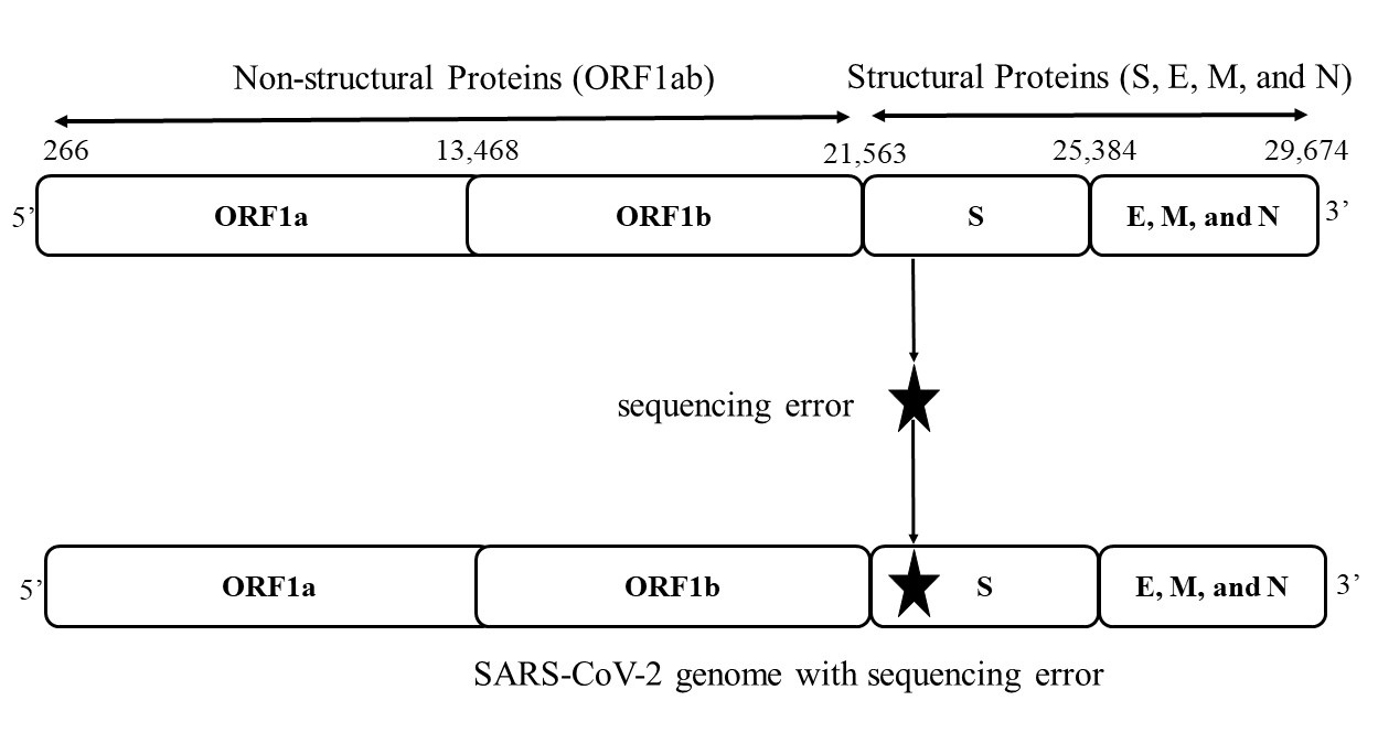
RNA viruses generally introduce errors during replication, the resulting mutations incorporated into the viral genome after repeated replication within a single host, generating a heterogeneous population of viral quasi-species. However, SARS-CoV-2 has an excellent proofreading mechanism that encodes a nonstructural protein 14 (nsp14) allowing it to have a -fold lower mutation rate than typical RNA viruses. Epidemiologists estimate that SARS-CoV-2 undergoes genomic mutations per year on average. Some of these mutations are advantageous, leading to more infectious variants of SARS-CoV-2 that continue to emerge [4]. Moreover, each major variant can be characterized or differentiated by a handful of mutations [5]. Hence, a sequencing error in the SARS-CoV-2 genome (see Figure 1) may lead to a false variant and influence the current study of SARS-CoV-2 virus [5, 6].
The diminishing cost of next-generation sequencing (NGS) technology has aided scientists from different parts of the world to generate large volumes of SARS-CoV-2 whole-genome sequencing (WGS) data. The Centers for Disease Control and Prevention (CDC) of the United States has also provided a wealth of information on resources, tools, and protocols for SARS-CoV-2 WGS data from different sequencing platforms such as Illumina, PacBio, and Ion Torrent. Finally, the Global Initiative on Sharing All Influenza Data (GISAID) hosts the largest SARS-CoV-2 genome sequencing dataset to date — the largest of any virus in history, with millions of sequences. This unprecedented amount of genomic data and easy availability allowed researchers to explore the molecular mechanism, genetic variability, evolutionary progress, and capability of development and spread of novel variants of the virus. On the other hand, this amount of data exceeds the capacity of the more traditional phylogenetic methods such as Nextstrain [9] or even the more recent IQTREE2 [10] by several orders of magnitude — a Big Data challenge. As a result, recent alternative approaches based on clustering and classification of sequences, e.g., to identify major variants have appeared in the literature [6, 11, 12, 13, 14], with promising accuracy and scalability properties.
Many issues still remain, however, such as sequencing errors being mistaken for mutations in different analyses when studying the evolutionary and transmission patterns of SARS-CoV-2 [15, 8], or other viruses. Incorporation of error in NGS sequences due to contamination in sample preparation, sequencing technology, or genome assembly methodology are other confounding factors. Generally, computational biologists filter those sequences having errors or mask those sequence fragments having errors. For example, each GISAID [16] sequence is a consensus sequence from the intra-host viral population sampled from the patient, averaging out the minor variations which exist in this population. While such a consensus sequence is a good representative of this population, i.e., it is still precise enough to capture the SARS-CoV-2 variant harbored by the infected individual, it comes at the cost of losing this important information, such as these minor variations. Such minor variations, when given enough time to evolve, e.g., within an immunocompromised individual can become dominant — one of the theories behind the emergence of the Alpha variant [17].
Many machine learning approaches towards clustering and classification of sequences [6, 12, 13, 14] have been operating under somewhat idealized conditions of virtually error-free consensus sequences, which may not be in certain settings. Moreover, some of these methods rely on a -mer based feature vector representation — an approach that does not even rely on alignment of the sequences, which may not always be available in certain settings, and can also introduce bias [18]. Such a framework should easily cope with errors as well — something machine learning approaches can do very naturally [19]. Hence, there is a great need for some way to reliably benchmark such methods for robustness to errors, which is what we carry out in this paper. Our main research question is the following:
How robust are the existing classification models to adversarial coronavirus inputs?
In this paper, we extend our error testing procedure as a framework for benchmarking the performance of different ML methods in terms of classification accuracy and robustness to different types of simulated nucleotide sequences with errors. This involves using PBSIM and InSilicoSeq tools for simulating long reads and short reads based nucleotide sequences with realistic error profiles.
We highlight the main contributions of this paper as follows:
-
•
We propose several ways of introducing biologically meaningful errors into the SARS-CoV-2 genome sequences, which reflect the error profiles of modern NGS technologies such as Illumina and PacBio.
-
•
We propose two different embedding methods, called PSSM2Vec (based on the concept of position weight matrix) and Min2Vec (based on the concept of minimizers), to generate a fixed length numerical representation of biological sequences. Using these embedding methods, we perform classification on original and errored sequences and report the performance using different evaluation metrics.
-
•
We show that the alignment free method for feature embedding, called Spike2Vec, which is based on the idea of -mers is better in terms of predictive performance when there is no error in the nucleotide sequences. This is likely due to the fact that it preserves nucleotide order information in more detail than the PSSM2Vec or Min2Vec representations (at the expense of being less compact).
-
•
We demonstrate that for the PBSIM (long reads) based errored sequences, that the PSSM2Vec embedding is more robust than the sliding window based Spike2Vec or Min2Vec approaches, possibly because it captures more long-range information.
-
•
We show that for the Illumina based errored sequences, Spike2Vec and Min2Vec are able to show better performance than PSSM2Vec, again because they likely preserve order information in higher detail.
This rest of the paper is organized as follows. In Section 2 we discuss related work. The methods to generate the adversarial examples is described in Section 3. In Section 4, we discuss different embedding methods used to convert the sequences into fixed-length numerical representation. Section 5 contains the details regarding the experimental setup, dataset statistics, and data visualization. We propose our results for accuracy and robustness in Section. 6. We described the limitations of our work in Section 7. Finally, we conclude this paper in Section 8.
2 Related Work
Assessing and benchmarking the robustness of ML or DL approaches by a series of adversarial attacks are popular in the image classification domain [20], but there are others that are closer to the domain of molecular data. In [21], the authors provide a series of realistic adversarial attacks to benchmark methods that predict chemical properties from atomistic simulations e.g., molecular conformation, reactions, and phase transitions. Even closer to the subject of our paper — protein sequences – the authors of [22] show that methods, such as AlphaFold [23] and RoseTTAFold [24] which employ deep neural networks to predict protein conformation are not robust: producing drastically different protein structures as a result of very small biologically meaningful perturbations in the protein sequence. Our approach is similar, albeit with a different goal of classification: namely, to explore how a small number of mutations (simulating the error introduced certain types of NGS technologies) can affect the downstream classification of different machine learning and deep learning approaches. After getting the numerical representation, a popular approach is to get the kernel matrix and give that matrix as input to traditional machine learning classifiers like support vector machines (SVM) [25, 26, 27]. However, these methods are expensive in terms of space complexity. Authors in [14, 6] propose an efficient embedding method for classification and clustering of spike sequences. However, their approaches are either not scalable or perform poorly on bigger datasets.
3 Adversarial Sequence Creation
We use two types of approaches to generate adversarial examples so that we can test the robustness of different machine learning methods.
3.1 PBSIM simulated data generation
PBSIM is developed to simulate Pacific Biosciences (PacBio) sequencing reads. Generally, the PacBio sequencer generates two types of reads: continuous long read (CLR) and circular consensus sequencing short reads (CCS). The CLR reads have a high error rate, and CCS reads have a lower error rate. PBSIM can simulate both CLR and CCS reads with different approaches: sampling-based simulation and model-based simulation. In the sampling-based simulation, PBSIM considers the length and quality of a provided read set to simulate the reads. In model-based simulation, PIBSIM simulates the reads on the basis of an error model [28].
To generate a sequence with errors, we take an original SARS-CoV-2 genomic sequence and simulate reads from it using the model-based approach, with the default PacBio error model. These reads (containing errors) are then aligned to the original sequence, mutations are called, and then consensus sequences (with mutations, some of which are errors) are extracted. We control the amount of error in the reads by adjusting the depth of the reads (a parameter of PBSIM). We generate such a sequence for 8220 different SARS-CoV-2 sequences from GISAID, for read depths 5 and 10 (more depths appear in the supplement).
3.2 InSilicoSeq simulated data generation
The InSilicoSeq open-source tool simulates the reads from different short read technologies such as Illumina. InSilicoSeq is a widely used tool, and several studies generate more realistic NGS data using this tool for planning new experiments and benchmarking purposes [29, 30, 31, 32, 33]. The tool can incorporate errors into the reads based on the details (e.g., chemistry) of recent Illumina platforms. InSilicoSeq supports substitution, insertion, and deletion errors and can model PHRED score. The current release of the InSilicoSeq tool has a pre-built error model for HiSeq, MiSeq, and NovaSeq instruments. Moreover, InSilicoSeq has the option to generate the number of reads according to the user’s requirement [34].
We generate a sequence with errors analogously to the above, this time controlling the error by adjusting this number of reads. We generate a sequence for the 8220 GISAID sequences mentioned above, with a number of reads 5000 and 10000 (with more numbers of reads in the supplement).
4 Feature Embeddings Generation
In this section, we introduce different feature embedding methods used to convert the nucleotide sequence into a fixed length representation.
4.1 Spike2Vec [14]
A popular approach to preserve the ordering of the sequential information, called Spike2Vec [14], takes the sliding window based substrings (called mers) of length (also called -gram). This -mers based representation helps to preserve the order of characters within the sequences [12] (see Figure 2 for example of -mers).
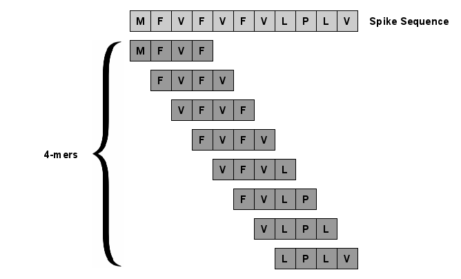
In this approach, first, the -mers are computed for each nucleotide sequence. Then a fixed length frequency vector is generated corresponding to each sequence, which contains the count of each -mer in that sequence. One advantage of using -mers based approach is that it is an “alignment free" method unlike other popular baselines (e.g. One-Hot Encoding “OHE" [6, 12]), which requires the sequences to be aligned. Note that sequence alignment is an expensive process and requires a reference sequence (genome) [35, 36]. It may also introduce bias into the result [18]. The total number of -mers in a given nucleotide sequences are , where is the length of the sequence. The variable is the user defined parameter. In this paper, we take (decided empirically using standard validation set approach [37]).
4.1.1 Frequency Vector Generation
After generating the -mers, the next step is to generate the fixed-length numerical representation (frequency vector) for the set of -mers in a nucleotide sequence. Suppose the set of nucleotides in the whole dataset is represented by alphabet (A, C, G, and T). Now, the length of the frequency vector will be (all possible combinations of -mers in of length ). In our dataset, since we have unique nucleotides in any sequence, the length of frequency vector in our case would be (when we take ).
4.2 PSSM2Vec
The PSSM2Vec embedding is based on the idea of Position Specific Scoring Matrix (PSSM), also called position weight matrix (PWM) [38, 39]. For a given nucleotide sequence , PSSM2Vec designs the PWM. The PWM generation start by first computing the -mers (where , which is decided using standard validation set approach [37]) for . For all the -mers in , a matrix of length is generated, which includes the count of nucleotides at different positions within the -mers. This matrix is also called the Position Frequency Matrix (PFM). In the next step, column wise probabilities are computed for PFM to get a new matrix, called the Position Probability Matrix (PPM). More formally, PPM is computed as follows: . To avoid having zero in the denominator, we add a small value of (called Laplace value or pseudocount) during probability computation. Finally, the PWM is computed from the PPM by taking the log likelihood of each nucleotide at a position . More formally:
| (1) |
where , which corresponds to the equal probability of occurrence for each nucleotide in the sequence. After generating the PWM, we flatten the matrix to generate a single vector, which we refer to as PSSM2Vec.
4.3 Min2Vec
The Min2Vec feature embedding is based on the idea of minimizers [40]. The minimizers is a modified version of -mers and used to represent the biological sequences in more compact form.
Definition 4.1 (Minimizers)
For a given -mer, a minimizer (also called m-mer) is a substring of consecutive nucleotides of length from the -mer, which is lexicographically smallest one in both forward and backward order of the k-mer, where and is fixed.
The pseudocode to compute the minimizers is given in Algorithm 1. For better understanding of pseudocode, we use the syntax of python code. To compute the minimizer, we take and , which is decided empirically using standard validation set approach [37]. After computing the minimizers for a given nucleotide sequence, we follow the same method to generate the frequency vector based representation as describe in Section 4.1.1. For reference, we call this method as Min2Vec.
5 Experimental Setup
All experiments are conducted using an Intel(R) Core i5 (11th generation) with GHz processor having windows ( bit) OS and GB memory. The simulated and pre-processed data is available online 111https://github.com/sarwanpasha/Adversarial_attack_on_biological_sequences. For classification purpose, we use Support Vector Machine (SVM), Naive Bayes (NB), Multi-Layer Perceptron (MLP), K-Nearest Neighbors (KNN), Random Forest (RF), Logistic Regression (LR), and Decision Tree (DT).
To measure the performance of ML models, we apply two different strategies. The first strategy is called Accuracy. In this case, we compute the average accuracy, precision, recall, F1 (weighted), F1 (Macro), and ROC-AUC for the whole (original) dataset without any errored sequence. The second strategy is called robustness. In this case, we only consider the adversarial examples (set of errored sequences) for the test set (and non errored sequences for training set) and compute average accuracy, precision, recall, F1 (weighted), F1 (Macro), and ROC-AUC for the ML models.
5.1 Dataset Statistics
We used the full length nucleotide sequences of coronavirus from a popular and publicly available database of SARS-CoV-2, GISAID 222https://www.gisaid.org/. In our dataset, we have nucleotide sequences along with the COVID-19 variant information. The total number of unique variants in our dataset are . The dataset statistics for the prepossessed data are given in Table 4 (in appendix). Our simulated dataset is available online 333https://drive.google.com/drive/folders/1adtr8FImIYTqxM20wgInRqIZ8EJY4HVS?usp=sharing for reproducibility. We also provide the visualization of different embedding methods (using t-SNE [41]) in Appendix B.
6 Results and Discussion
In this section, we show the accuracy results for the original data followed by the robustness results of PBSIM and Illumina based errored sequences.
6.1 Accuracy Results
To evaluate the performance of original nucleotide sequences (non-errored sequences), we split the original sequences into (random) training and testing set and perform classification on different embedding methods. We ran the experiments 5 times and report average results. The accuracy results for different embeddings and ML models are shown in Table 1. We can observe that the SVM classifiers with Spike2Vec based embedding outperform other embeddings and ML models for all but one evaluation metrics. In terms of runtime, since the length of vectors for PSSM2Vec is smaller than the other embedding methods, its training runtime for NB classifier is the smallest one.
| Embed. Method | ML Algo. | Acc. | Prec. | Recall | F1 weigh. | F1 Macro | ROC- AUC | Train. runtime (sec.) |
|---|---|---|---|---|---|---|---|---|
| Spike2Vec | SVM | 0.87 | 0.87 | 0.87 | 0.86 | 0.76 | 0.87 | 7.43 |
| NB | 0.03 | 0.05 | 0.03 | 0.02 | 0.05 | 0.55 | 0.09 | |
| MLP | 0.75 | 0.74 | 0.75 | 0.74 | 0.36 | 0.68 | 18.42 | |
| KNN | 0.73 | 0.73 | 0.73 | 0.71 | 0.48 | 0.71 | 2.04 | |
| RF | 0.82 | 0.85 | 0.82 | 0.80 | 0.67 | 0.78 | 2.17 | |
| LR | 0.86 | 0.85 | 0.86 | 0.85 | 0.70 | 0.84 | 8.67 | |
| DT | 0.67 | 0.67 | 0.67 | 0.66 | 0.42 | 0.71 | 0.27 | |
| PSSM2Vec | SVM | 0.28 | 0.08 | 0.28 | 0.12 | 0.01 | 0.50 | 3.14 |
| NB | 0.01 | 0.01 | 0.01 | 0.00 | 0.01 | 0.52 | 0.03 | |
| MLP | 0.34 | 0.27 | 0.34 | 0.26 | 0.06 | 0.53 | 17.31 | |
| KNN | 0.32 | 0.28 | 0.32 | 0.28 | 0.13 | 0.55 | 0.33 | |
| RF | 0.33 | 0.30 | 0.33 | 0.31 | 0.16 | 0.57 | 1.60 | |
| LR | 0.28 | 0.08 | 0.28 | 0.12 | 0.01 | 0.50 | 0.68 | |
| DT | 0.29 | 0.28 | 0.29 | 0.28 | 0.13 | 0.56 | 0.06 | |
| Min2Vec | SVM | 0.60 | 0.58 | 0.60 | 0.56 | 0.48 | 0.72 | 15.19 |
| NB | 0.05 | 0.12 | 0.05 | 0.04 | 0.12 | 0.59 | 0.08 | |
| MLP | 0.57 | 0.52 | 0.57 | 0.53 | 0.30 | 0.64 | 26.32 | |
| KNN | 0.55 | 0.56 | 0.55 | 0.53 | 0.37 | 0.66 | 1.51 | |
| RF | 0.75 | 0.79 | 0.75 | 0.74 | 0.61 | 0.76 | 1.72 | |
| LR | 0.58 | 0.55 | 0.58 | 0.54 | 0.40 | 0.68 | 6.36 | |
| DT | 0.64 | 0.64 | 0.64 | 0.64 | 0.48 | 0.74 | 0.14 |
6.2 Robustness Results
For the robustness results, we show the predictive performance of different ML models by first using the PBSIM based adversarial sequences and then show the performance of ML models for Illumina based adversarial examples.
For the PBSIM based sequences, we take the original (non-errored) sequence data for training the ML models and use the PBSIM based () errored sequences as the test set. The purpose of this experimental setting is to evaluate the performance of ML models on the errored sequences, which were not available during the training process. In this experimental setting, we show the results for depth and depth based errored sequences (in test set) in Table 2.
| Depth: 5 | Depth: 10 | ||||||||||||||
|---|---|---|---|---|---|---|---|---|---|---|---|---|---|---|---|
| Embed. Method | ML Algo. | Acc. | Prec. | Recall | F1 weigh. | F1 Macro | ROC- AUC | Train. runtime (sec.) | Acc. | Prec. | Recall | F1 weigh. | F1 Macro | ROC- AUC | Train. runtime (sec.) |
| Spike2Vec | SVM | 0.01 | 0.00 | 0.01 | 0.00 | 0.00 | 0.50 | 16.48 | 0.01 | 0.00 | 0.01 | 0.00 | 0.00 | 0.50 | 16.88 |
| NB | 0.00 | 0.00 | 0.00 | 0.00 | 0.00 | 0.50 | 0.68 | 0.00 | 0.00 | 0.00 | 0.00 | 0.00 | 0.50 | 0.71 | |
| MLP | 0.28 | 0.08 | 0.28 | 0.12 | 0.01 | 0.50 | 23.65 | 0.02 | 0.00 | 0.02 | 0.00 | 0.00 | 0.50 | 16.86 | |
| KNN | 0.28 | 0.08 | 0.28 | 0.12 | 0.01 | 0.50 | 1.68 | 0.28 | 0.08 | 0.28 | 0.12 | 0.01 | 0.50 | 1.78 | |
| RF | 0.28 | 0.08 | 0.28 | 0.12 | 0.01 | 0.50 | 1.78 | 0.28 | 0.08 | 0.28 | 0.12 | 0.01 | 0.50 | 2.88 | |
| LR | 0.01 | 0.00 | 0.01 | 0.00 | 0.00 | 0.50 | 11.30 | 0.01 | 0.00 | 0.01 | 0.00 | 0.00 | 0.50 | 12.04 | |
| DT | 0.01 | 0.00 | 0.01 | 0.00 | 0.00 | 0.50 | 0.34 | 0.01 | 0.00 | 0.01 | 0.00 | 0.00 | 0.50 | 0.36 | |
| PSSM2Vec | SVM | 0.27 | 0.07 | 0.27 | 0.11 | 0.01 | 0.50 | 8.14 | 0.30 | 0.09 | 0.30 | 0.13 | 0.01 | 0.50 | 8.32 |
| NB | 0.27 | 0.07 | 0.27 | 0.11 | 0.01 | 0.50 | 0.34 | 0.30 | 0.09 | 0.30 | 0.13 | 0.01 | 0.50 | 0.36 | |
| MLP | 0.27 | 0.07 | 0.27 | 0.11 | 0.01 | 0.50 | 7.47 | 0.30 | 0.09 | 0.30 | 0.13 | 0.01 | 0.50 | 7.90 | |
| KNN | 0.27 | 0.07 | 0.27 | 0.11 | 0.01 | 0.50 | 0.51 | 0.01 | 0.05 | 0.01 | 0.00 | 0.00 | 0.50 | 0.52 | |
| RF | 0.27 | 0.07 | 0.27 | 0.11 | 0.01 | 0.50 | 1.17 | 0.30 | 0.09 | 0.30 | 0.13 | 0.01 | 0.50 | 0.98 | |
| LR | 0.27 | 0.07 | 0.27 | 0.11 | 0.01 | 0.50 | 3.76 | 0.30 | 0.09 | 0.30 | 0.13 | 0.01 | 0.50 | 3.62 | |
| DT | 0.27 | 0.07 | 0.27 | 0.11 | 0.01 | 0.50 | 0.02 | 0.30 | 0.09 | 0.30 | 0.13 | 0.01 | 0.50 | 0.02 | |
| Min2Vec | SVM | 0.27 | 0.07 | 0.26 | 0.11 | 0.01 | 0.50 | 5.22 | 0.27 | 0.08 | 0.27 | 0.12 | 0.01 | 0.50 | 4.91 |
| NB | 0.26 | 0.07 | 0.27 | 0.11 | 0.26 | 0.50 | 0.43 | 0.27 | 0.08 | 0.27 | 0.12 | 0.01 | 0.50 | 0.34 | |
| MLP | 0.26 | 0.07 | 0.26 | 0.11 | 0.26 | 0.50 | 1.63 | 0.27 | 0.08 | 0.27 | 0.12 | 0.01 | 0.50 | 1.92 | |
| KNN | 0.26 | 0.07 | 0.26 | 0.11 | 0.26 | 0.50 | 0.62 | 0.08 | 0.01 | 0.08 | 0.01 | 0.00 | 0.50 | 0.69 | |
| RF | 0.26 | 0.07 | 0.26 | 0.11 | 0.26 | 0.50 | 0.67 | 0.27 | 0.08 | 0.27 | 0.12 | 0.01 | 0.50 | 0.77 | |
| LR | 0.26 | 0.07 | 0.26 | 0.11 | 0.26 | 0.50 | 0.69 | 0.27 | 0.08 | 0.27 | 0.12 | 0.01 | 0.50 | 0.67 | |
| DT | 0.26 | 0.07 | 0.26 | 0.11 | 0.26 | 0.50 | 0.17 | 0.27 | 0.08 | 0.27 | 0.12 | 0.01 | 0.50 | 0.26 | |
For the Illumina based sequences, we take the original (non-errored) sequence data for training the ML models and use the illumina based errored sequences as the test set. In this experimental setting, we show the results for sequences simulated using different number of short reads (in test set). The results for short reads and short reads based errored sequences are shown in Table 3.
| # of Short Reads: 5000 | # of Short Reads: 10000 | ||||||||||||||
| Embed. Method | ML Algo. | Acc. | Prec. | Recall | F1 weigh. | F1 Macro | ROC- AUC | Train. runtime (sec.) | Acc. | Prec. | Recall | F1 weigh. | F1 Macro | ROC- AUC | Train. runtime (sec.) |
| Spike2Vec | SVM | 0.68 | 0.66 | 0.68 | 0.66 | 0.49 | 0.73 | 6.75 | 0.73 | 0.72 | 0.71 | 0.72 | 0.55 | 0.76 | 10.76 |
| NB | 0.69 | 0.73 | 0.69 | 0.71 | 0.57 | 0.80 | 0.31 | 0.72 | 0.72 | 0.72 | 0.72 | 0.53 | 0.77 | 0.32 | |
| MLP | 0.68 | 0.65 | 0.68 | 0.66 | 0.34 | 0.66 | 75.93 | 0.68 | 0.65 | 0.68 | 0.66 | 0.32 | 0.65 | 27.84 | |
| KNN | 0.73 | 0.73 | 0.73 | 0.72 | 0.57 | 0.76 | 0.75 | 0.73 | 0.72 | 0.73 | 0.72 | 0.56 | 0.76 | 0.68 | |
| RF | 0.72 | 0.72 | 0.72 | 0.70 | 0.51 | 0.72 | 2.44 | 0.73 | 0.73 | 0.73 | 0.71 | 0.55 | 0.74 | 2.43 | |
| LR | 0.72 | 0.70 | 0.72 | 0.70 | 0.52 | 0.74 | 6.71 | 0.72 | 0.71 | 0.72 | 0.71 | 0.54 | 0.75 | 6.69 | |
| DT | 0.51 | 0.53 | 0.51 | 0.52 | 0.32 | 0.66 | 0.24 | 0.56 | 0.56 | 0.56 | 0.56 | 0.41 | 0.70 | 0.21 | |
| PSSM2Vec | SVM | 0.27 | 0.07 | 0.27 | 0.12 | 0.01 | 0.50 | 8.20 | 0.28 | 0.08 | 0.28 | 0.12 | 0.01 | 0.50 | 9.64 |
| NB | 0.01 | 0.00 | 0.01 | 0.00 | 0.01 | 0.51 | 0.39 | 0.02 | 0.01 | 0.02 | 0.01 | 0.03 | 0.52 | 0.25 | |
| MLP | 0.32 | 0.22 | 0.32 | 0.24 | 0.06 | 0.52 | 10.30 | 0.34 | 0.25 | 0.34 | 0.26 | 0.08 | 0.53 | 12.72 | |
| KNN | 0.26 | 0.21 | 0.26 | 0.22 | 0.06 | 0.52 | 1.10 | 0.29 | 0.26 | 0.29 | 0.25 | 0.09 | 0.54 | 0.70 | |
| RF | 0.30 | 0.24 | 0.30 | 0.25 | 0.08 | 0.52 | 2.17 | 0.32 | 0.25 | 0.32 | 0.27 | 0.08 | 0.53 | 1.92 | |
| LR | 0.27 | 0.07 | 0.27 | 0.12 | 0.01 | 0.50 | 3.92 | 0.28 | 0.08 | 0.28 | 0.12 | 0.01 | 0.50 | 3.26 | |
| DT | 0.30 | 0.24 | 0.30 | 0.25 | 0.07 | 0.52 | 0.12 | 0.32 | 0.25 | 0.32 | 0.26 | 0.08 | 0.53 | 0.07 | |
| Min2Vec | SVM | 0.52 | 0.47 | 0.52 | 0.46 | 0.30 | 0.64 | 11.75 | 0.54 | 0.50 | 0.54 | 0.49 | 0.34 | 0.66 | 7.45 |
| NB | 0.05 | 0.27 | 0.05 | 0.04 | 0.09 | 0.63 | 0.20 | 0.07 | 0.37 | 0.07 | 0.08 | 0.14 | 0.64 | 0.19 | |
| MLP | 0.52 | 0.46 | 0.52 | 0.46 | 0.26 | 0.62 | 25.0 | 0.52 | 0.46 | 0.52 | 0.48 | 0.25 | 0.62 | 28.70 | |
| KNN | 0.55 | 0.55 | 0.55 | 0.53 | 0.39 | 0.67 | 0.52 | 0.57 | 0.57 | 0.57 | 0.56 | 0.47 | 0.70 | 0.56 | |
| RF | 0.65 | 0.67 | 0.65 | 0.63 | 0.46 | 0.70 | 1.75 | 0.68 | 0.69 | 0.68 | 0.66 | 0.56 | 0.74 | 1.60 | |
| LR | 0.51 | 0.46 | 0.51 | 0.46 | 0.28 | 0.63 | 2.91 | 0.53 | 0.49 | 0.53 | 0.48 | 0.34 | 0.65 | 2.90 | |
| DT | 0.47 | 0.47 | 0.47 | 0.47 | 0.31 | 0.65 | 0.12 | 0.54 | 0.54 | 0.54 | 0.54 | 0.42 | 0.70 | 0.10 | |
6.3 PBSIM vs Illumina Results Discussion
Third generation sequencing technologies such as PacBio and Oxford Nanopore Technologies (ONT), being newer than traditional high-throughput NGS technologies (e.g., Illumina), offer longer reads, which are useful to efforts such as haplotype assembly [42, 43]. The drawback with these technologies is that they have lower coverage and contain more errors — up to error rate as compared to the less than with state-of-the-art Illiumina [44, 45, 46, 47]. Therefore, it is not surprising that perturbing the coverage in the case of Pacbio (PBSIM) based experiment had a larger effect (see Table 2) on the predictive performance of ML models as compared to the Illumina (insilicoseq) based experiment (see Table 3). The sequences submitted to GISAID 444https://www.gisaid.org/ database are almost exclusively from high-throughput technologies [16], hence we got more stable results on the original sequences (without adding any additional error) extracted from GISAID (see Table 1).
For the PBSIM based errored sequences, we can observe that PSSM2Vec outperforms the other two embedding methods (see Table 2), which means that a sliding window based approach (using -mers or -mers) is not desirable while dealing with Pacbio errors. This could be due to the fact that the PSSM2Vec representation captures more long-range information than the shorter (length ) sliding window. Similarly, for the Illumina based sequences, we can observe the opposite behavior (see Table 3), where the sliding window based approaches are better than the position weight matrix based embedding. This could be because in PSSM2Vec, the order of nucleotides is not preserved in as much detail (because we just take the position weight matrix and make it a 1-D vector by flattening it). In the sliding window based approach, the majority of the nucleotides appear in sliding windows, hence preserving more (order) information, which results in better predictive performance (because of less loss of information in generating the numerical embedding). This comes at the cost of it being a higher dimensional representation, of course.
7 Limitations
We used feature engineering based embeddings for the experiments in this paper. However, using neural network could improve the accuracy and/or robustness of the benchmark dataset. Moreover, we use the Illumina based data with and short reads only — we believe that using a larger number of reads may improve the performance of the underlying classifier. The same is true for PBSIM data where we use only 5 and 10 as read depth. Please note that results on more number of short reads (for illumina) and read depth (for PBSIM) are given in the supplementary material file.
8 Conclusion
In this paper, we propose two different ways to test the robustness of ML models in terms of sequence classification. We test the accuracy and robustness of ML models using different embedding methods. We conclude that for different simulation tools, different embedding methods perform better than the others and there is no clear winner, which consistently outperforms in all scenarios. One interesting future extension is to use other embedding methods from the literature and also apply deep learning models for classification of sequences. Studying adversarial attack on other viruses (e.g. Zika) is also an interesting future extension.
References
- [1] F. Wu, S. Zhao, B. Yu, Y.-M. Chen, W. Wang, Z.-G. Song, Y. Hu, Z.-W. Tao, J.-H. Tian, Y.-Y. Pei et al., “A new coronavirus associated with human respiratory disease in china,” Nature, vol. 579, no. 7798, pp. 265–269, 2020.
- [2] S. E. Park, “Epidemiology, virology, and clinical features of severe acute respiratory syndrome-coronavirus-2 (sars-cov-2; coronavirus disease-19),” Clinical and experimental pediatrics, vol. 63, no. 4, p. 119, 2020.
- [3] Y.-Z. Zhang and E. C. Holmes, “A genomic perspective on the origin and emergence of sars-cov-2,” Cell, vol. 181, no. 2, pp. 223–227, 2020.
- [4] M. I. Nelson, “Tracking the uk sars-cov-2 outbreak,” Science, vol. 371, no. 6530, pp. 680–681, 2021.
- [5] SARS-CoV-2 Variant Classifications and Definitions, https://www.cdc.gov/coronavirus/2019-ncov/variants/variant-info.html, 2021, [Online; accessed 1-September-2021].
- [6] K. Kuzmin et al., “Machine learning methods accurately predict host specificity of coronaviruses based on spike sequences alone,” Biochemical and Biophysical Research Communications, vol. 533, pp. 553–558, 2020.
- [7] Y. Huang, C. Yang, X.-f. Xu, W. Xu, and S.-w. Liu, “Structural and functional properties of sars-cov-2 spike protein: potential antivirus drug development for covid-19,” Acta Pharmacologica Sinica, vol. 41, no. 9, pp. 1141–1149, 2020.
- [8] M. M. Arons, K. M. Hatfield, S. C. Reddy, A. Kimball, A. James, J. R. Jacobs, J. Taylor, K. Spicer, A. C. Bardossy, L. P. Oakley et al., “Presymptomatic sars-cov-2 infections and transmission in a skilled nursing facility,” New England journal of medicine, vol. 382, no. 22, pp. 2081–2090, 2020.
- [9] J. Hadfield, C. Megill, S. Bell, J. Huddleston, B. Potter, C. Callender, P. Sagulenko, T. Bedford, and R. Neher, “Nextstrain: real-time tracking of pathogen evolution,” Bioinformatics, vol. 34, pp. 4121–4123, 2018.
- [10] B. Q. Minh et al., “Iq-tree 2: New models and efficient methods for phylogenetic inference in the genomic era,” Molecular Biology and Evolution, vol. 37, no. 5, pp. 1530–1534, 2020.
- [11] A. Melnyk, F. Mohebbi, S. Knyazev, B. Sahoo, R. Hosseini, P. Skums, A. Zelikovsky, and M. Patterson, “Clustering based identification of sars-cov-2 subtypes,” in International Conference on Computational Advances in Bio and Medical Sciences. Springer, 2020, pp. 127–141.
- [12] S. Ali, B. Sahoo, N. Ullah, A. Zelikovskiy, M. Patterson, and I. Khan, “A k-mer based approach for sars-cov-2 variant identification,” in International Symposium on Bioinformatics Research and Applications. Springer, 2021, pp. 153–164.
- [13] S. Ali, Tamkanat-E-Ali, M. A. Khan, I. Khan, and M. Patterson, “Effective and scalable clustering of sars-cov-2 sequences,” in International Conference on Big Data Research (ICBDR), 2021, pp. 1–8.
- [14] S. Ali and M. Patterson, “Spike2vec: An efficient and scalable embedding approach for covid-19 spike sequences,” in International Conference on Big Data (Big Data), 2021, pp. 1533–1540.
- [15] GISAID History, https://www.gisaid.org/about-us/history/, 2021, [Online; accessed 4-October-2021].
- [16] GISAID Website, https://www.gisaid.org/, 2021, [Online; accessed 09-June-2022].
- [17] D. Frampton, T. Rampling, A. Crosss, H. Bailey, J. Heaney, M. Byott et al., “Genomic characteristics and clinical effect of the emergent sars-cov-2 b.1.1.7 lineage in london, uk: a whole-genome sequencing and hospital-based cohort study,” The Lancet Infectious Diseases, vol. 21, pp. 1246–1256, 2021.
- [18] T. Golubchik, M. J. Wise, S. Easteal, and L. S. Jermiin, “Mind the Gaps: Evidence of Bias in Estimates of Multiple Sequence Alignments,” Molecular Biology and Evolution, vol. 24, no. 11, pp. 2433–2442, 08 2007. [Online]. Available: https://doi.org/10.1093/molbev/msm176
- [19] N. Du, J. Shang, and Y. Sun, “Improving protein domain classification for third-generation sequencing reads using deep learning,” BMC Genomics, vol. 22, no. 251, 2021.
- [20] D. Hendrycks and T. Dietterich, “Benchmarking neural network robustness to common corruptions and perturbations,” arXiv, 2019.
- [21] D. Schwalbe-Koda, A. Tan, and R. Gómez-Bombarelli, “Differentiable sampling of molecular geometries with uncertainty-based adversarial attacks,” Nature Communications, vol. 12, no. 5104, 2021.
- [22] S. K. Jha, A. Ramanathan, R. Ewetz, A. Velasquez, and S. Jha, “Protein folding neural networks are not robust,” arXiv, 2021.
- [23] J. Jumper et al., “Highly accurate protein structure prediction with AlphaFold,” Nature, 2021.
- [24] M. Baek et al., “Accurate prediction of protein structures and interactions using a 3-track network,” bioRxiv, 2021.
- [25] C. Leslie, E. Eskin, J. Weston, and W. Noble, “Mismatch string kernels for svm protein classification,” in Advances in neural information processing systems (NeurIPS), 2003, pp. 1441–1448.
- [26] M. Farhan, J. Tariq, A. Zaman, M. Shabbir, and I. Khan, “Efficient approximation algorithms for strings kernel based sequence classification,” in Advances in neural information processing systems (NeurIPS). ., 2017, pp. 6935–6945.
- [27] P. Kuksa, I. Khan, and V. Pavlovic, “Generalized similarity kernels for efficient sequence classification,” in SIAM International Conference on Data Mining (SDM), 2012, pp. 873–882.
- [28] Y. Ono, K. Asai, and M. Hamada, “Pbsim: Pacbio reads simulator—toward accurate genome assembly,” Bioinformatics, vol. 29, pp. 119–121, 11 2012.
- [29] K. L. Kalantar, T. Carvalho, C. F. A. de Bourcy, B. Dimitrov, G. Dingle, R. Egger, J. Han, O. B. Holmes, Y.-F. Juan, R. King, A. Kislyuk, M. F. Lin, M. Mariano, T. Morse, L. V. Reynoso, D. R. Cruz, J. Sheu, J. Tang, J. Wang, M. A. Zhang, E. Zhong, V. Ahyong, S. Lay, S. Chea, J. A. Bohl, J. E. Manning, C. M. Tato, and J. L. DeRisi, “Idseq—an open source cloud-based pipeline and analysis service for metagenomic pathogen detection and monitoring,” GigaScience, vol. 9, 10 2020.
- [30] M. Sangiovanni, I. Granata, A. S. Thind, and M. R. Guarracino, “From trash to treasure: detecting unexpected contamination in unmapped ngs data,” BMC Bioinformatics, vol. 20, 04 2019.
- [31] A. Whibley, J. L. Kelley, and S. R. Narum, “The changing face of genome assemblies: Guidance on achieving high-quality reference genomes,” Molecular Ecology Resources, vol. 21, pp. 641–652, 01 2021.
- [32] S. Andreu-Sánchez, L. Chen, D. Wang, H. E. Augustijn, A. Zhernakova, and J. Fu, “A benchmark of genetic variant calling pipelines using metagenomic short-read sequencing,” Frontiers in Genetics, vol. 12, 05 2021.
- [33] C. Glickman, J. Hendrix, and M. Strong, “Simulation study and comparative evaluation of viral contiguous sequence identification tools,” BMC Bioinformatics, vol. 22, 06 2021.
- [34] H. Gourlé, O. Karlsson-Lindsjö, J. Hayer, and E. Bongcam-Rudloff, “Simulating illumina metagenomic data with insilicoseq,” Bioinformatics, vol. 35, pp. 521–522, 07 2018.
- [35] B. Chowdhury and G. Garai, “A review on multiple sequence alignment from the perspective of genetic algorithm,” Genomics, vol. 109, no. 5-6, pp. 419–431, 2017.
- [36] L. Denti, Y. Pirola, M. Previtali, T. Ceccato, G. Della Vedova, R. Rizzi, and P. Bonizzoni, “Shark: fishing relevant reads in an rna-seq sample,” Bioinformatics, vol. 37, no. 4, pp. 464–472, 2021.
- [37] P. Devijver and J. Kittler, “Pattern recognition: A statistical approach,” in London, GB: Prentice-Hall, 1982, pp. 1–448.
- [38] G. D. Stormo, T. D. Schneider, L. Gold, and A. Ehrenfeucht, “Use of the ’perceptron’ algorithm to distinguish translational initiation sites in e. coli,” Nucleic Acids Research, vol. 10, no. 9, 1982.
- [39] S. Ali, B. Bello, P. Chourasia, R. T. Punathil, Y. Zhou, and M. Patterson, “Pwm2vec: An efficient embedding approach for viral host specification from coronavirus spike sequences,” MDPI Biology, 2022.
- [40] M. Roberts, W. Haynes, B. Hunt, S. Mount, and J. Yorke, “Reducing storage requirements for biological sequence comparison,” Bioinformatics, vol. 20, pp. 3363–9, 2004.
- [41] L. Van der M. and G. Hinton, “Visualizing data using t-sne.” Journal of Machine Learning Research (JMLR), vol. 9, no. 11, 2008.
- [42] M. Patterson*, T. Marschall*, N. Pisanti, L. van Iersel, L. Stougie, G. W. Klau†, and A. Schonhuth†, “WhatsHap: Weighted haplotype assembly for future-generation sequencing reads,” Journal of Computational Biology, vol. 22, no. 6, pp. 498–509, 2015.
- [43] S. Beretta*, M. Patterson*, S. Zaccaria, G. D. Vedova, and P. Bonizzoni, “HapCHAT: Adaptive haplotype assembly for efficiently leveraging high coverage in long reads,” BMC Bioinformatics, vol. 19, no. 252, 2018.
- [44] J. L. Weirather, M. de Cesare, Y. Wang, P. Piazza, V. Sebastiano, X.-J. Wang, D. Buck, and K. F. Au, “Comprehensive comparison of pacific biosciences and oxford nanopore technologies and their applications to transcriptome analysis,” F1000Research, vol. 6, 06 2017. [Online]. Available: https://www.ncbi.nlm.nih.gov/pmc/articles/PMC5553090/
- [45] S. Fu, A. Wang, and K. F. Au, “A comparative evaluation of hybrid error correction methods for error-prone long reads,” Genome Biology, vol. 20, 02 2019.
- [46] N. Stoler and A. Nekrutenko, “Sequencing error profiles of illumina sequencing instruments,” NAR Genomics and Bioinformatics, vol. 3, 01 2021.
- [47] X. Ma, Y. Shao, L. Tian, D. A. Flasch, H. L. Mulder, M. N. Edmonson, Y. Liu, X. Chen, S. Newman, J. Nakitandwe, Y. Li, B. Li, S. Shen, Z. Wang, S. Shurtleff, L. L. Robison, S. Levy, J. Easton, and J. Zhang, “Analysis of error profiles in deep next-generation sequencing data,” Genome Biology, vol. 20, 03 2019.
Appendix A Appendix A: Dataset Statistics
The information regarding the number of variants (used as class labels) in our data are given in Table 4.
| Variant | Num. of sequences | Variant | Num. of sequences |
|---|---|---|---|
| AY.103 | 2271 | AY.121 | 40 |
| AY.44 | 1416 | AY.75 | 37 |
| AY.100 | 717 | AY.3.1 | 30 |
| AY.3 | 710 | AY.3.3 | 28 |
| AY.25 | 585 | AY.107 | 27 |
| AY.25.1 | 382 | AY.34.1 | 25 |
| AY.39 | 248 | AY.46.6 | 21 |
| AY.119 | 242 | AY.98.1 | 20 |
| B.1.617.2 | 175 | AY.13 | 19 |
| AY.20 | 130 | AY.116.1 | 18 |
| AY.26 | 107 | AY.126 | 17 |
| AY.4 | 100 | AY.114 | 15 |
| AY.117 | 94 | AY.125 | 14 |
| AY.113 | 94 | AY.34 | 14 |
| AY.118 | 86 | AY.46.1 | 14 |
| AY.43 | 85 | AY.92 | 13 |
| AY.122 | 84 | AY.98 | 12 |
| BA.1 | 79 | AY.46.4 | 12 |
| AY.119.2 | 74 | AY.127 | 12 |
| AY.47 | 73 | AY.111 | 10 |
| AY.39.1 | 70 | _ | _ |
Appendix B Appendix B: Data Visualization
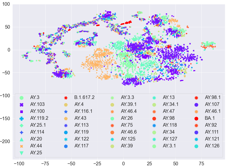
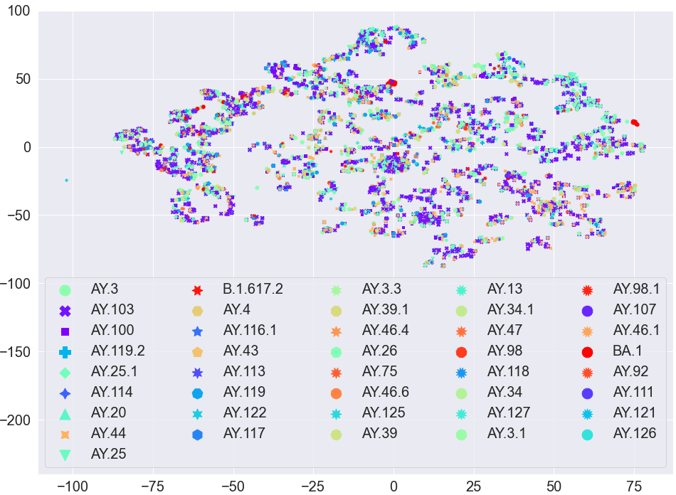
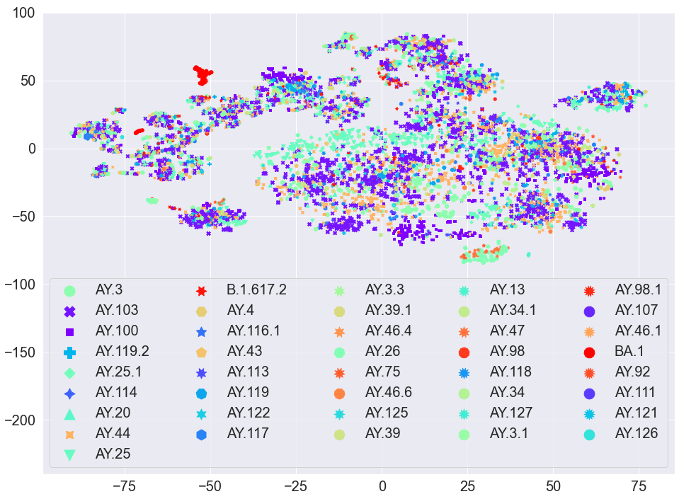
To visualise if there is any (natural) clustering in our data, we generated 2d representation of the feature embeddings using t-distributed stochastic neighbor embedding (t-SNE) approach [41]. The main advantage of t-SNE is that it preserves the pair-wise distance between vectors in dimensions. The t-SNE plot for different coronavirus variants is given in Figure 3(a), Figure 3(b), and Figure 3(c) for Spike2Vec, PSSM2Vec, and Min2Vec, respectively. For Spike2Vec based t-SNE plot, we can observe that some of the variants (e.g. AY.103) is grouped more clearly than the other variants. PSSM2Vec however maintains smaller groups of variants as compared to Spike2Vec. The structure of Min2Vec based t-SNE is more similar to Spike2Vec, however, it grouped some other variants (e.g. AY.96.1) more clearly as compared to Spike2Vec. In general, we can observe that all embedding methods preserves the overall structure of the data.
Appendix C Appendix C: Results and Discussion
The standard deviation of runs for the original data (without any errored sequences) is given in Table 5. Note the the accuracies (average values of runs) for the same data are reported in Table 1 in the main paper.
| Embed. Method | ML Algo. | Acc. | Prec. | Recall | F1 weigh. | F1 Macro | ROC- AUC | Train. runtime (sec.) |
|---|---|---|---|---|---|---|---|---|
| Spike2Vec | SVM | 0.009337 | 0.008654 | 0.009337 | 0.009122 | 0.011612 | 0.011101 | 0.300614 |
| NB | 0.003307 | 0.059135 | 0.003307 | 0.003323 | 0.002726 | 0.007099 | 0.017888 | |
| MLP | 0.012523 | 0.015917 | 0.012523 | 0.015363 | 0.028586 | 0.017015 | 3.836258 | |
| KNN | 0.009530 | 0.011883 | 0.009530 | 0.010848 | 0.022703 | 0.011329 | 0.036290 | |
| RF | 0.005541 | 0.006865 | 0.005541 | 0.006641 | 0.028757 | 0.014456 | 0.263474 | |
| LR | 0.005504 | 0.004573 | 0.005504 | 0.005868 | 0.017053 | 0.012580 | 0.867295 | |
| DT | 0.004102 | 0.002976 | 0.004102 | 0.003101 | 0.013446 | 0.010527 | 0.032883 | |
| PSSM2Vec | SVM | 0.007223 | 0.003972 | 0.007223 | 0.005558 | 0.000217 | 0.000000 | 0.118888 |
| NB | 0.002015 | 0.007148 | 0.002015 | 0.000983 | 0.004011 | 0.006194 | 0.008142 | |
| MLP | 0.005716 | 0.015879 | 0.005716 | 0.006257 | 0.009698 | 0.005917 | 2.603367 | |
| KNN | 0.009810 | 0.013064 | 0.009810 | 0.010757 | 0.023313 | 0.010837 | 0.028786 | |
| RF | 0.006478 | 0.008212 | 0.006478 | 0.007973 | 0.017069 | 0.007942 | 0.052490 | |
| LR | 0.007223 | 0.003972 | 0.007223 | 0.005558 | 0.000217 | 0.000000 | 0.025634 | |
| DT | 0.006273 | 0.009446 | 0.006273 | 0.007321 | 0.013302 | 0.007477 | 0.009866 | |
| Min2Vec | SVM | 0.008510 | 0.008449 | 0.009629 | 0.008932 | 0.015522 | 0.010247 | 0.281588 |
| NB | 0.004464 | 0.060411 | 0.004464 | 0.006046 | 0.02021 | 0.007911 | 0.016351 | |
| MLP | 0.011599 | 0.007398 | 0.011599 | 0.009882 | 0.028691 | 0.015814 | 1.480781 | |
| KNN | 0.006601 | 0.009581 | 0.006601 | 0.007661 | 0.014181 | 0.005275 | 0.014744 | |
| RF | 0.004837 | 0.004967 | 0.004837 | 0.006467 | 0.034441 | 0.017324 | 0.044175 | |
| LR | 0.001902 | 0.005262 | 0.001902 | 0.002995 | 0.014008 | 0.004733 | 0.261828 | |
| DT | 0.010011 | 0.011210 | 0.010011 | 0.010262 | 0.024173 | 0.014445 | 0.011970 |
C.1 Robustness Results on Errored Sequences
The robustness results of PBSIM based errored sequences (with depth and ) are shown in Table 6. Similarly the robustness results with Illumina based errored sequences having number of short reads as and are shown in Table 7.
| Depth: 15 | Depth: 20 | ||||||||||||||
|---|---|---|---|---|---|---|---|---|---|---|---|---|---|---|---|
| Embed. Method | ML Algo. | Acc. | Prec. | Recall | F1 weigh. | F1 Macro | ROC- AUC | Train. runtime (sec.) | Acc. | Prec. | Recall | F1 weigh. | F1 Macro | ROC- AUC | Train. runtime (sec.) |
| Spike2Vec | SVM | 0.01 | 0.00 | 0.01 | 0.00 | 0.00 | 0.50 | 11.19 | 0.01 | 0.00 | 0.01 | 0.00 | 0.00 | 0.50 | 11.17 |
| NB | 0.00 | 0.00 | 0.00 | 0.00 | 0.00 | 0.50 | 0.81 | 0.00 | 0.00 | 0.00 | 0.00 | 0.00 | 0.50 | 0.70 | |
| MLP | 0.00 | 0.00 | 0.00 | 0.00 | 0.00 | 0.50 | 21.66 | 0.01 | 0.00 | 0.01 | 0.00 | 0.00 | 0.50 | 20.82 | |
| KNN | 0.28 | 0.08 | 0.28 | 0.12 | 0.01 | 0.50 | 2.32 | 0.28 | 0.08 | 0.28 | 0.12 | 0.01 | 0.50 | 2.24 | |
| RF | 0.28 | 0.08 | 0.28 | 0.12 | 0.01 | 0.50 | 2.48 | 0.28 | 0.08 | 0.28 | 0.12 | 0.01 | 0.50 | 2.42 | |
| LR | 0.01 | 0.00 | 0.01 | 0.00 | 0.00 | 0.50 | 11.89 | 0.01 | 0.00 | 0.01 | 0.00 | 0.00 | 0.50 | 11.77 | |
| DT | 0.01 | 0.00 | 0.01 | 0.00 | 0.00 | 0.50 | 0.31 | 0.01 | 0.00 | 0.01 | 0.00 | 0.00 | 0.50 | 0.31 | |
| PSSM2Vec | SVM | 0.28 | 0.08 | 0.28 | 0.12 | 0.01 | 0.50 | 9.97 | 0.28 | 0.08 | 0.28 | 0.12 | 0.01 | 0.50 | 9.54 |
| NB | 0.01 | 0.00 | 0.01 | 0.00 | 0.00 | 0.50 | 0.15 | 0.01 | 0.00 | 0.01 | 0.00 | 0.00 | 0.50 | 0.16 | |
| MLP | 0.01 | 0.00 | 0.01 | 0.00 | 0.00 | 0.50 | 15.63 | 0.01 | 0.00 | 0.01 | 0.00 | 0.00 | 0.50 | 19.20 | |
| KNN | 0.01 | 0.00 | 0.01 | 0.00 | 0.00 | 0.50 | 2.21 | 0.01 | 0.00 | 0.01 | 0.00 | 0.00 | 0.50 | 2.18 | |
| RF | 0.00 | 0.00 | 0.00 | 0.00 | 0.00 | 0.50 | 2.03 | 0.00 | 0.00 | 0.00 | 0.00 | 0.00 | 0.50 | 1.94 | |
| LR | 0.28 | 0.08 | 0.28 | 0.12 | 0.01 | 0.50 | 1.13 | 0.28 | 0.08 | 0.28 | 0.12 | 0.01 | 0.50 | 1.11 | |
| DT | 0.00 | 0.00 | 0.00 | 0.00 | 0.00 | 0.50 | 0.09 | 0.00 | 0.00 | 0.00 | 0.00 | 0.00 | 0.50 | 0.08 | |
| Min2Vec | SVM | 0.01 | 0.01 | 0.01 | 0.00 | 0.01 | 0.50 | 15.47 | 0.01 | 0.01 | 0.01 | 0.00 | 0.01 | 0.50 | 17.54 |
| NB | 0.00 | 0.00 | 0.00 | 0.00 | 0.00 | 0.50 | 0.77 | 0.00 | 0.00 | 0.00 | 0.00 | 0.00 | 0.50 | 0.84 | |
| MLP | 0.05 | 0.00 | 0.05 | 0.00 | 0.00 | 0.50 | 24.19 | 0.05 | 0.00 | 0.05 | 0.00 | 0.00 | 0.50 | 34.86 | |
| KNN | 0.05 | 0.00 | 0.05 | 0.00 | 0.00 | 0.50 | 2.50 | 0.05 | 0.00 | 0.05 | 0.00 | 0.00 | 0.50 | 1.93 | |
| RF | 0.09 | 0.01 | 0.09 | 0.01 | 0.00 | 0.50 | 2.39 | 0.28 | 0.08 | 0.28 | 0.12 | 0.01 | 0.50 | 2.25 | |
| LR | 0.00 | 0.00 | 0.00 | 0.00 | 0.00 | 0.50 | 9.45 | 0.00 | 0.00 | 0.00 | 0.00 | 0.00 | 0.50 | 10.11 | |
| DT | 0.07 | 0.01 | 0.07 | 0.01 | 0.00 | 0.50 | 0.20 | 0.07 | 0.01 | 0.07 | 0.01 | 0.00 | 0.50 | 0.19 | |
| # of Short Reads: 15000 | # of Short Reads: 20000 | ||||||||||||||
| Embed. Method | ML Algo. | Acc. | Prec. | Recall | F1 weigh. | F1 Macro | ROC- AUC | Train. runtime (sec.) | Acc. | Prec. | Recall | F1 weigh. | F1 Macro | ROC- AUC | Train. runtime (sec.) |
| Spike2Vec | SVM | 0.68 | 0.69 | 0.68 | 0.67 | 0.44 | 0.72 | 12.41 | 0.68 | 0.69 | 0.68 | 0.67 | 0.44 | 0.72 | 11.60 |
| NB | 0.00 | 0.00 | 0.00 | 0.00 | 0.03 | 0.52 | 0.95 | 0.00 | 0.00 | 0.00 | 0.00 | 0.03 | 0.52 | 0.65 | |
| MLP | 0.63 | 0.64 | 0.63 | 0.62 | 0.32 | 0.67 | 26.30 | 0.63 | 0.65 | 0.63 | 0.63 | 0.31 | 0.66 | 20.25 | |
| KNN | 0.51 | 0.50 | 0.51 | 0.45 | 0.13 | 0.56 | 2.50 | 0.51 | 0.50 | 0.51 | 0.45 | 0.13 | 0.56 | 2.29 | |
| RF | 0.71 | 0.73 | 0.71 | 0.68 | 0.51 | 0.71 | 3.17 | 0.71 | 0.72 | 0.71 | 0.68 | 0.49 | 0.71 | 2.64 | |
| LR | 0.71 | 0.70 | 0.71 | 0.69 | 0.47 | 0.73 | 12.22 | 0.71 | 0.70 | 0.71 | 0.69 | 0.47 | 0.73 | 12.22 | |
| DT | 0.53 | 0.55 | 0.53 | 0.53 | 0.35 | 0.68 | 0.33 | 0.52 | 0.54 | 0.52 | 0.52 | 0.31 | 0.66 | 0.32 | |
| PSSM2Vec | SVM | 0.28 | 0.08 | 0.28 | 0.12 | 0.01 | 0.50 | 9.79 | 0.28 | 0.08 | 0.28 | 0.12 | 0.01 | 0.50 | 9.59 |
| NB | 0.00 | 0.00 | 0.00 | 0.00 | 0.00 | 0.50 | 0.18 | 0.00 | 0.00 | 0.00 | 0.00 | 0.00 | 0.50 | 0.22 | |
| MLP | 0.22 | 0.20 | 0.22 | 0.14 | 0.03 | 0.51 | 15.89 | 0.18 | 0.18 | 0.18 | 0.14 | 0.02 | 0.51 | 19.92 | |
| KNN | 0.17 | 0.22 | 0.17 | 0.14 | 0.02 | 0.51 | 1.98 | 0.17 | 0.22 | 0.17 | 0.14 | 0.02 | 0.51 | 2.28 | |
| RF | 0.12 | 0.17 | 0.12 | 0.12 | 0.03 | 0.51 | 1.76 | 0.13 | 0.18 | 0.13 | 0.13 | 0.03 | 0.51 | 2.00 | |
| LR | 0.28 | 0.08 | 0.28 | 0.12 | 0.01 | 0.50 | 1.01 | 0.28 | 0.08 | 0.28 | 0.12 | 0.01 | 0.50 | 1.03 | |
| DT | 0.13 | 0.19 | 0.13 | 0.13 | 0.03 | 0.51 | 0.09 | 0.12 | 0.18 | 0.12 | 0.12 | 0.03 | 0.51 | 0.08 | |
| Min2Vec | SVM | 0.52 | 0.53 | 0.52 | 0.48 | 0.31 | 0.65 | 19.16 | 0.52 | 0.54 | 0.52 | 0.48 | 0.32 | 0.65 | 18.63 |
| NB | 0.02 | 0.07 | 0.02 | 0.01 | 0.06 | 0.55 | 0.95 | 0.02 | 0.07 | 0.02 | 0.01 | 0.06 | 0.55 | 0.77 | |
| MLP | 0.50 | 0.45 | 0.50 | 0.45 | 0.22 | 0.59 | 33.36 | 0.52 | 0.48 | 0.52 | 0.48 | 0.29 | 0.63 | 37.64 | |
| KNN | 0.37 | 0.35 | 0.37 | 0.31 | 0.10 | 0.55 | 2.42 | 0.37 | 0.35 | 0.37 | 0.31 | 0.10 | 0.55 | 2.34 | |
| RF | 0.64 | 0.68 | 0.64 | 0.60 | 0.46 | 0.69 | 2.21 | 0.64 | 0.67 | 0.64 | 0.60 | 0.45 | 0.69 | 2.44 | |
| LR | 0.51 | 0.53 | 0.51 | 0.46 | 0.30 | 0.64 | 9.14 | 0.51 | 0.53 | 0.51 | 0.46 | 0.30 | 0.64 | 9.38 | |
| DT | 0.51 | 0.53 | 0.51 | 0.51 | 0.35 | 0.68 | 0.19 | 0.51 | 0.53 | 0.51 | 0.51 | 0.36 | 0.68 | 0.19 | |