Cooling with fermionic reservoir

Abstract

Recently, much emphasis has been given to genuinely quantum reservoirs generically called fermionic reservoirs. These reservoirs are characterized by having finite levels, as opposed to bosonic reservoirs, which have infinite levels that can be populated via an increase in temperature. Given this, some studies are being carried out to explore the advantages of using quantum reservoirs, in particular in the operation of heat machines. In this work, we make a comparative study of a thermal refrigerator operating in the presence of either a bosonic or a fermionic reservoir, and we show that fermionic reservoirs have advantages over bosonic ones. We propose an explanation for the origin of these advantages by analyzing both the asymptotic behavior of the states of the qubits and the exchange rates between these qubits and their respective reservoirs.

I Introduction

With the development of quantum thermodynamics (Gemmer et al., 2004; Binder et al., 2019; Strasberg and Winter, 2021), there is an increasing interest in the realization of thermal devices operating at the quantum limit (Abah et al., 2012; Alicki, 2014; Alecce et al., 2015; Roßnagel et al., 2016; Camati et al., 2019; Erdman et al., 2019; Chen et al., 2019). In particular, heat engines whose working substance consists of systems with finite levels of energy, such as two-level systems, can absorb from or deliver to their surroundings quantities of energy as small as their corresponding energy gaps. In contrast, bosonic working substances, modeled by quantum harmonic oscillators, have infinitely many levels, where higher and higher levels can be populated by increasing temperature. Comparative studies exploring the difference between a bosonic and a fermionic working substance demonstrate that there are advantages in considering working substances with finite levels for quantum engines (Henrich et al., 2007; de Assis et al., 2020; Mendes et al., 2021; El Makouri et al., 2022). In particular, systems with finite energy levels, such as two-level systems, can exhibit stationary states with population inversion (Carr, 2013; Braun et al., 2013; de Assis et al., 2019a), giving rise to absolute negative temperatures (Abraham and Penrose, 2017; Struchtrup, 2018). The population inversion associated with negative temperatures of the system requires thermal reservoirs built with fermionic substances, as experimentally demonstrated in (Carr, 2013; Braun et al., 2013; Mendonça et al., 2020). This inverted population effect has been explored in some works (Landsberg et al., 1980; Xi and Quan, 2017; Mendonça et al., 2020), with remarkable impact on the efficiency of heat engines, as experimentally shown in Ref. (de Assis et al., 2019a; Mendonça et al., 2020). On the other hand, fermionic reservoirs (Artacho and Falicov, 1993; Henrich et al., 2007; Álvarez et al., 2010; Linden et al., 2010; Li and Jia, 2011; Nüßeler et al., 2020; Del Re et al., 2020; Mikhailov and Troshkin, 2020) built with two-level substances whose energy gap is $E$ does not necessarily need to present population inversion, in which case its temperature $T$ remains positive, with the average excitation number given by the Fermi-Dirac distribution $n=1/\left(e^{E/T}+1\right)<0.5$, in contrast with bosonic substances where the average excitation number is given by the Bose-Einstein distribution $n=1/\left(e^{E/T}-1\right)$. In the condition of positive temperature, one could imagine that there would be no gain in considering fermionic reservoirs. However, in this work we consider a study of case in which a refrigerator built with two-level substances can present advantages when operating in a fermionic environment as compared to a bosonic one, with both environments at positive temperatures. As the operating conditions are kept the same for both environments, our results emphasize that the presented advantage stems from the quantum nature of the fermionic reservoir.

II Model

In the present work, we consider a self-contained quantum refrigerator (SCQR) composed of three interacting qubits, each in contact with a specific thermal reservoir. This SCQR was first proposed in Ref. (Linden et al., 2010), in which the authors took into account only bosonic reservoirs. Recently, we investigated this SCQR operating with one of the reservoirs being a fermionic one at a negative temperature, see Ref. (Damas et al., 2022). Here, as in Ref. (Linden et al., 2010), we approach the case in which qubits 1, 2, and 3 interact respectively with a thermal reservoir at a cold temperature $T_{c}>0$, a thermal reservoir at a "room" temperature $T_{r}>0$, and a thermal reservoir at a hot temperature $T_{h}>0$ - see the schematic shown in Fig. 1. The device in question works like a refrigerator when $T_{1}-T_{c}<0$, where $T_{1}$ is the temperature of qubit 1. In this case, therefore, heat flows from the cold reservoir to qubit 1. However, considering the asymptotic state, this only occurs if the relations $E_{3}=E_{2}-E_{1}$, with $E_{k}$ being the energy gap of qubit $k$ ($k=1,2,3$), and $T_{c}<T_{r}<T_{h}$ are satisfied (Linden et al., 2010).

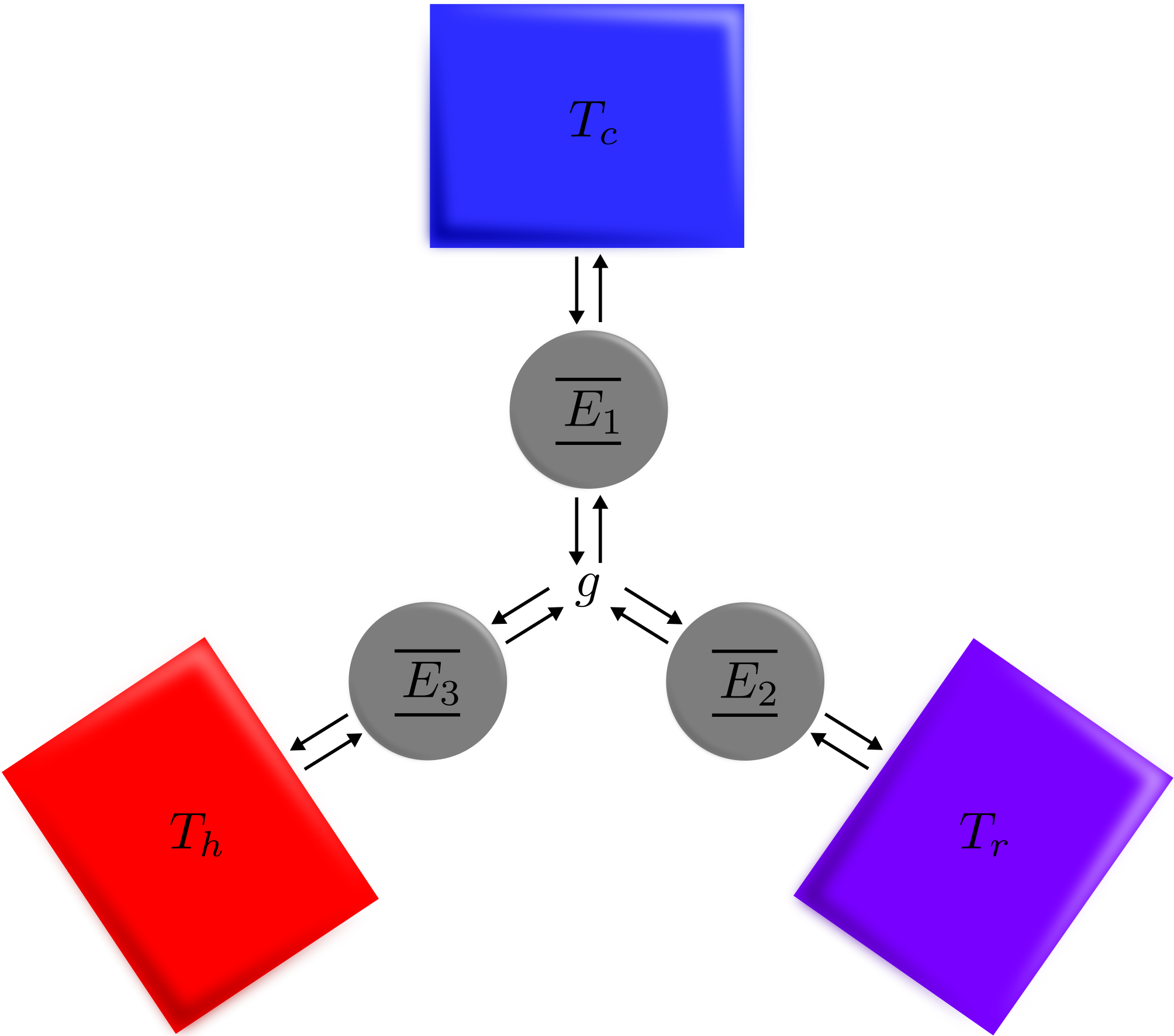
Figure 1: Schematic representation of the SCQR refrigerator and its respective thermal reservoirs. The SCQR is composed of three interacting qubits having energy gaps $E_{1},E_{2}$, and $E_{3}$ in contact with their respective reservoirs. Here, $T_{h}$ is the temperature of the hot reservoir, $T_{r}$ is the temperature of the "room" reservoir, $T_{c}$ is the temperature of the cold reservoir, and g is the coupling constant between the qubits.

We assume the weak coupling limit and the Markovian regime governing the dynamics of the SCQR, such that the master equation is (Breuer et al., 2002; Li and Jia, 2011)

$$\frac{d\rho}{dt}=-i\left[H_{0}+H_{int}\right]+\\ \sum_{k=1}^{3}\Gamma_{B\left(F\right),k}^{\downarrow}\left(\sigma_{-,k}\rho\sigma_{+,k}-\frac{1}{2}\left\{\sigma_{+,k}\sigma_{-,k},\rho\right\}\right)+\\ \sum_{k=1}^{3}\Gamma_{B\left(F\right),k}^{\uparrow}\left(\sigma_{+,k}\rho\sigma_{-,k}-\frac{1}{2}\left\{\sigma_{-,k}\sigma_{+,k},\rho\right\}\right).$$ (1)

Here, the free qubits Hamiltonian $H_{0}$ and the three-body interaction Hamiltonian $H_{int}$ are given by

$$H_{0}=\frac{1}{2}E_{1}\sigma_{z,1}+\frac{1}{2}E_{3}\sigma_{z,3}+\frac{1}{2}E_{3}\sigma_{z,3}$$ (2)

and

$$H_{int}=g\left(\sigma_{-,1}\sigma_{+,2}\sigma_{-,3}+\sigma_{+,1}\sigma_{-,2}\sigma_{+,3}\right),$$ (3)

where $\sigma_{z,k}$ is the z Pauli operator for qubit $k$, $g$ is the coupling constant, and $\sigma_{-,k}$ ($\sigma_{+,k}$) is the lowering (raising) Pauli operator for qubit $k$. Note that Eq. (1) governs the dynamics of either bosonic (Breuer et al., 2002) and fermionic (Artacho and Falicov, 1993; Álvarez et al., 2010; Li and Jia, 2011) thermal reservoirs: if qubit $k$ is interacting with a bosonic (fermionic) thermal reservoir, $\Gamma_{B,k}^{\downarrow}=\gamma_{k}\left(1+n_{B,k}\right)$ ($\Gamma_{F,k}^{\downarrow}=\gamma_{k}\left(1-n_{F,k}\right)$) and $\Gamma_{B,k}^{\uparrow}=\gamma_{k}n_{B,k}$ ($\Gamma_{F,k}^{\uparrow}=\gamma_{k}n_{F,k}$), where $\gamma_{k}$ is the dissipation rate and $n_{B,k}=1/(\text{e}^{E_{k}/T_{\phi_{k}}}-1)$ ($n_{F,k}=1/(\text{e}^{E_{k}/T_{\phi_{k}}}+1)$) is the average excitation number, being $\phi_{1}=c$, $\phi_{2}=r$, and $\phi_{3}=h$. Note that since for bosons $\Gamma_{B,k}^{\downarrow}=\gamma_{k}\left(1+n_{B,k}\right)$, $\Gamma_{B,k}^{\uparrow}=\gamma_{k}n_{B,k}$ and for fermions the average excitation number is limited to 0.5 for positive temperatures, then $\Gamma_{B,k}^{\downarrow}$ and $\Gamma_{B,k}^{\uparrow}$ is always greater than $\Gamma_{F,k}^{\downarrow}$ and $\Gamma_{F,k}^{\uparrow}$. To obtain the asymptotic state of Eq. (1) we used the quantum optics toolbox (Johansson et al., 2012, 2013).

III Results

To compare the SCQR operating in the different configurations involving bosonic and fermionic reservoirs, we start by fixing the energies $E_{1}=1$, $E_{2}=5$, and $E_{3}=4$; the temperatures $T_{c}=1,1.5,2$, and $T_{r}=2$; the coupling constant $g=10^{-2}$; and the dissipation rates $\gamma_{1}=\gamma_{2}=\gamma_{3}=g$. Next, we let $T_{h}$ vary from $10^{-1}$ to $10^{3}$.

Fig. 2(a) shows the temperature difference $T_{1}-T_{c}$ versus $T_{h}$ (on logarithmic scale) for the SCQR working in a bosonic environment for the cold temperatures $T_{c}=1$ (dotted green line), $T_{c}=1.5$ (dashed red line), and $T_{c}=2$ (solid blue line). As said before, cooling occurs when $T_{1}-T_{c}<0$. Similarly, Fig. 2(b) shows $T_{1}-T_{c}$ as a function of $T_{h}$ for the same cold temperatures, but now the SCQR is surrounded by fermionic reservoirs. In Fig. 2(a), $T_{1}-T_{c}$ decreases to a minimum value and then increases until it stabilizes at a negative value close to zero, while, in Fig. 2(b), $T_{1}-T_{c}$ stabilizes at its minimum value. Thus, the SCQR in the fermionic environment has an advantage over the bosonic one, as its efficiency in cooling qubit 1 does not decrease at higher values of $T_{h}$. Furthermore, under fermionic reservoirs, qubit 1 reaches lower minimum temperature values than when under bosonic reservoirs, as can be seen from the difference $T_{1}-T_{c}$, which is more negative for the fermionic environment (compare Figs. 2(a) and 2(b)).

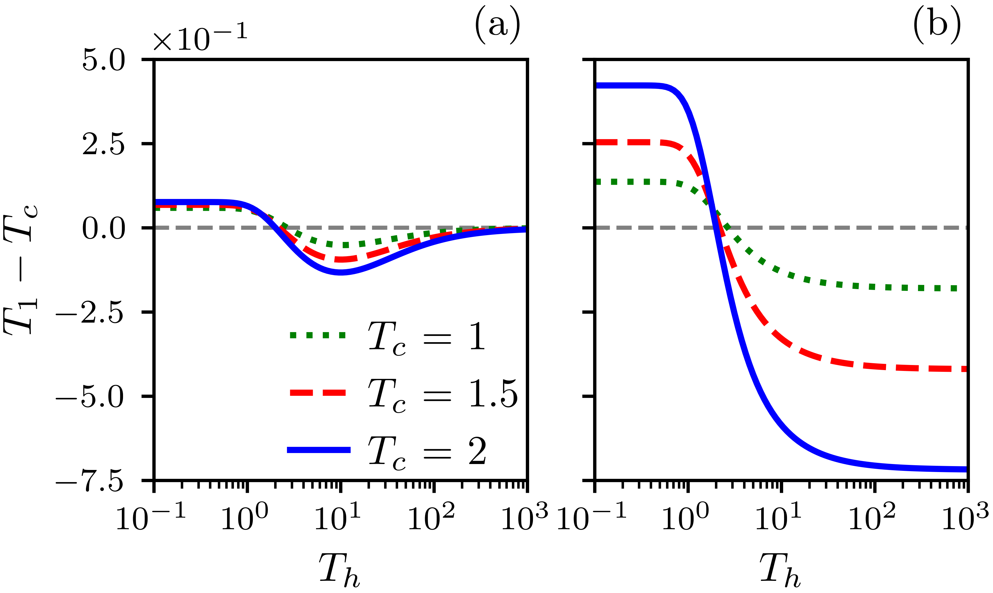
Figure 2: Temperature difference $T_{1}-T_{c}$ versus $T_{h}$ for (a) three bosonic and (b) three fermionic reservoirs, considering three different values of $T_{c}$: $T_{c}=1$ (dotted green line), $T_{c}=1.5$ (dashed red line) and $T_{c}=2$ (solid blue line). Refrigeration occurs for $T_{1}-T_{c}<0$. Note the difference in behavior in the two figures: while in (a) temperature $T_{1}$ reaches a minimum and then starts to increase, in (b) $T_{1}$ decreases monotonically, practically stabilizing for sufficiently high $T_{h}$, thus indicating that the lowest temperatures reached by qubit 1 occur for fermionic reservoirs.

According to our numerical simulations, when considering the bosonic environment, the minimum values for $T_{1}$ are $T_{1}=0.95$ (when $T_{c}=1$), $T_{1}=1.41$ (when $T_{c}=1.5$), and $T_{1}=1.87$ (when $T_{c}=2$). On the other hand, when considering three fermionic reservoirs, since the values for $T_{1}$ continue to decrease with increasing $T_{h}$, we take the minimum value for $T_{1}$ when $T_{h}=100$. These minimum values are $T_{1}=0.82$ (when $T_{c}=1$), $T_{1}=1.09$ (when $T_{c}=1.5$), and $T_{1}=1.29$ (when $T_{c}=2$). By considering $T_{c}$ as a reference we can then calculate the cooling percentage $\left(\left|T_{1}-T_{c}\right|/T_{c}\right)\times 100$ to compare how much the fermionic and bosonic reservoirs cools qubit 1 - see Tab. 1, where 3B (3F) stands for three bosonic (fermionic) reservoirs.

$T_{c}$		(%)
		3B	3F
1		5.14	17.57
1.5		6.31	27.44
2		6.65	35.32

Table 1: Comparative values in the cooling percentage $\left(\left|T_{1}-T_{c}\right|/T_{c}\right)\times 100$ for the refrigerator working at three bosonic (3B) and three fermionic (3F) reservoirs for three values of the reference temperature $T_{c}$.

Tab. 1 shows a significant difference in the cooling percentage for the two sets of reservoirs: it is always higher when using three fermionic reservoirs, thus clearly showing that the fermionic environment is far more efficient in decreasing the temperature $T_{1}$ than the bosonic one. Also, this percentage is better the higher the reference temperature $T_{c}$, such that for $T_{c}=2$, it can reach up to more than four times the value reached using only bosonic reservoirs. For lower values of the cold temperatures $T_{c}$, the percentage difference decreases but using fermionic reservoirs, the cooling when $T_{c}=1$ is still more than double that of the case of bosonic reservoirs alone. It is worth mentioning that by fixing the SCQR parameters as we did, there is a limit to cooling qubit 1. As we found numerically, the corresponding lowest cooling percentage reached by qubit 1, irrespective of the type of reservoir used, occurs when $T_{c}\sim 0.48$. For temperatures lower than $T_{c}\sim 0.48$, $T_{1}-T_{c}>0$, meaning that the SCQR no longer works. Also, the percentage of cooling decreases more and more as $T_{c}$ approaches $0.48$ for both reservoirs. However, the percentage of cooling when using fermionic reservoirs remains higher, as shown in Tab. 2.

$T_{c}$		(%)
		3B	3F
0.48		0.87	3.31
0.60		2.20	7.39
0.80		4.14	12.85

Table 2: Comparative values show that the cooling percentages $\left(\left|T_{1}-T_{c}\right|/T_{c}\right)\times 100$ for fixed parameters decrease as the reference temperature $T_{c}$ approaches $0.48$, where $T_{1}-T_{c}>0$. Note that even so fermionic reservoirs are always more effective for cooling.

As we have seen, for fixed parameters we cannot cool down qubit 1 to zero absolute. However, there is a strategy to keep up cooling toward zero absolute, which is to isolate qubit 1 from its environment. This condition, obtained by imposing $\gamma_{1}\rightarrow 0$ or equivalently $\Gamma_{B\left(F\right),1}^{\downarrow}\rightarrow 0$ and $\Gamma_{B\left(F\right),1}^{\uparrow}\rightarrow 0$ in (1), allows us to obtain the following analytical solution for the temperature of qubit 1:

$$T_{1}=\frac{T_{c}}{1+\frac{E_{3}}{E_{1}}\left(1-\frac{T_{c}}{T_{h}}\right)},$$ (4)

from which we can see that, if we let $E_{3}/E_{1}\rightarrow\infty$, then $T_{1}\rightarrow 0$. This result, obtained in Ref. (Linden et al., 2010), shows that there is no fundamental limit to cool down to zero absolute, provided we can perfectly isolate qubit 1.

So far we have considered fermionic reservoirs for all qubits in the SCQR. Other possibilities include the cases of combinations of bosonic and fermionic reservoirs. In fact, considering the fermionic reservoir as a quantum resource, it may be interesting to consider cases where only one or two fermionic reservoirs are used. For this, it is necessary to consider which qubit the fermionic reservoir is associated with. Let us use a notation in which B (F) denotes the bosonic (fermionic) reservoir and the order in which it appears in the sequence indicates which qubit that reservoir is attached to. For example, the sequence BFB indicates that qubit 1 is subjected to a bosonic reservoir, qubit 2 to a fermionic reservoir, and the third qubit to a bosonic reservoir. Next, we investigate all configurations numerically and grouped the results in Tab. 3, ordering from highest to lowest percentage of cooling and following the same procedure as in the previous tables, i.e., we took the minimum value for $T_{1}$.

$T_{c}$		(%)
		FBF	FFF	FBB	FFB	BBF	BFF	BBB	BFB
0.48		3.38	3.31	1.11	1.10	2.71	2.65	0.87	0.86
0.80		13.09	12.85	7.31	7.22	7.76	7.62	4.14	4.09
1		17.87	17.57	10.81	10.67	9.03	8.87	5.14	5.09
1.5		27.28	27.44	18.65	18.43	10.28	10.13	6.31	6.24
2		35.76	35.32	25.36	25.09	10.46	10.33	6.65	6.58

Table 3: Comparative values showing the cooling percentages $\left(\left|T_{1}-T_{c}\right|/T_{c}\right)\times 100$ for several reservoir configurations. Here, for example, BFF means qubit 1 bound to a bosonic reservoir and qubits 2 and 3 bound to fermionic reservoirs. Note that the highest percentage of cooling occurs for FBF configuration, meaning that qubit 1 is bound to a fermionic reservoir, qubit 2 is bound to a bosonic reservoir and qubit 3 is bound to another fermionic reservoir.

Interestingly, and c ontrary to what one might think, the best case does not occur when three fermionic reservoirs are used. As Tab. 3 shows, the greatest cooling range occurs for FBF case, i.e., when only qubit 1 and 3 are bound to fermionic reservoirs. Although the difference between the FBF and FFF configurations is small, it is still notable that the cooling percentage is higher when only two fermionic reservoirs are used instead of three.

	FBF	FFF	FBB	FFB	BBF	BFF	BBB	BFB
$\Gamma_{B\left(F\right),1}^{\downarrow}$	0.00622	0.00622	0.00622	0.00622	0.02541	0.02541	0.02541	0.02541
$\Gamma_{B\left(F\right),1}^{\uparrow}$	0.00378	0.00378	0.00378	0.00378	0.01541	0.01541	0.01541	0.01541
$\Gamma_{B\left(F\right),2}^{\downarrow}$	0.01089	0.00924	0.01089	0.00924	0.01089	0.00924	0.01089	0.00924
$\Gamma_{B\left(F\right),2}^{\uparrow}$	0.00089	0.00076	0.00089	0.00076	0.00089	0.00076	0.00089	0.00076
$\Gamma_{B\left(F\right),3}^{\downarrow}$	0.00510	0.00510	0.02812	0.02812	0.00510	0.00510	0.02812	0.02812
$\Gamma_{B\left(F\right),3}^{\uparrow}$	0.00490	0.00490	0.01812	0.01812	0.00490	0.00490	0.01812	0.01812

Table 4: Exchange rates $\Gamma_{B\left(F\right),k}^{\downarrow}$ and $\Gamma_{B\left(F\right),k}^{\uparrow}$ of the qubit k with their respective reservoirs. From this Table, we see that the lowest (highest) exchange rates occur for fermionic (bosonic) reservoirs. Note that the FBF configuration presents the smallest exchange rates for qubit 1. This explains why it is more effective for cooling qubit 1 - see main text. The temperatures used are $T_{c}=2$, $T_{r}=2$, and $T_{h}$ varies to minimize the values of $T_{1}$, as the SCQR behavior changes as shown in Figs. 2(a) and 2(b). The same pattern occurs if we use other values for $T_{c}$.

In this regard, note that the FFB and BFF sequences, although each also contain only two fermionic reservoirs and one bosonic reservoir, they have a lower cooling percentage than that of the FBF sequence. For instance, for $T_{c}=2$, the cooling percentage of FBF is $29.72\%$, which is higher than that for sequence FFB ($25.09\%$) and BFF ($10.33\%$). The explanation for this fact is given below. Remembering that the lowest temperature for qubit 1, which is the qubit we want to cool, occurs when it is completely isolated, it is to be expected, therefore, that when the exchange rates $\Gamma_{F(B),1}^{\uparrow}$ and $\Gamma_{F(B),1}^{\downarrow}$ of qubit 1 with its reservoir are the lowest possible, the cooling will take place more effectively, with perfect insulation being the best case. In Tab. 4 we show the exchange rates $\Gamma_{F(B),k}^{\uparrow}$ and $\Gamma_{F(B),k}^{\downarrow}$, $k=1,2,3$, for the k-th qubit for temperatures $T_{c}=2$, $T_{r}=2$, and $T_{h}=10$. From Tab. 4 we see that the $\Gamma_{F(B),1}^{\uparrow}$ and $\Gamma_{F(B),1}^{\downarrow}$ rates are the smallest whenever the sequence starts with F, and remain the smallest irrespective of the temperatures used, according to our simulations. Another relevant point to be considered, which we have already shown in Figs. 2(a) is that bosonic reservoirs have the disadvantage of making the cooling non-monotonic, and therefore less effective. Thus, obtaining better cooling percentages requires that the last reservoir be fermionic, as we also verified in our numerical simulations. The role of the nature of the second reservoir and its relevance to cooling percentages is quite complex. In our numerical simulations, we were able to identify that the best cooling percentages occur, whenever one bosonic reservoir and two fermionic reservoirs are used, in the sequence FBF - see Tab. 3. Regarding other configurations with lower cooling percentages but yet involving two fermionic and one bosonic reservoir, note for example that the FFB sequence may have higher or lower cooling percentages than the BFF sequence depending on whether the temperature $T_{c}$ is higher or lower than unity.

IV Conclusion

Recent studies on heat machines have used quantum reservoirs as a resource to obtain better performances both in engines and in refrigerators (Landsberg et al., 1980; Xi and Quan, 2017; de Assis et al., 2019b, 2020). For example, fermionic reservoirs have been explored in previous works, especially in their purely quantum characteristic of presenting population inversion (de Assis et al., 2019a; Mendonça et al., 2020), which, in turn, is associated with negative effective temperatures (Abraham and Penrose, 2017; Strasberg and Winter, 2021). Here we explore the quantum nature of fermionic reservoirs without taking population inversion into account, such that we restrict to the domain of positive temperatures. Using a qubit-based refrigerator model proposed in Ref. (Linden et al., 2010), we show that, once the operating parameters of the refrigerator are fixed, the use of fermionic reservoirs allows to obtain better results, with respect to the cooling capacity, than the use of bosonic reservoirs. We have verified, for example, that when the qubit to be cooled cannot be perfectly insulated, the use of only fermionic reservoirs allows to reach lower temperatures than the use of only bosonic reservoirs. In addition, contrary to what might be thought, the cooling can be more effective, in the sense of obtaining a higher percentage of cooling, when instead of three, only two fermionic reservoirs are used. We show that an explanation of this somewhat unexpected result is due to the exchanged rates between qubit 1 and its reservoir as well as to the behavior of the asymptotic cooling of qubit 1 when subjected to different types of reservoirs. In summary, when the condition for perfect insulation cannot be reached, our results unequivocally demonstrate the superiority of the fermionic reservoir in the process of cooling qubits to the lowest possible temperatures.