Contrastive Environmental Sound Representation Learning

Machine hearing of the environmental sound is one of the important issues in the audio recognition domain. It gives the machine the ability to discriminate between the different input sounds that guides its decision making. In this work we exploit the self-supervised contrastive technique and a shallow 1D CNN to extract the distinctive audio features (audio representations) without using any explicit annotations.We generate representations of a given audio using both its raw audio waveform and spectrogram and evaluate if the proposed learner is agnostic to the type of audio input. We further use canonical correlation analysis (CCA) to fuse representations from the two types of input of a given audio and demonstrate that the fused global feature results in robust representation of the audio signal as compared to the individual representations. The evaluation of the proposed technique is done on both ESC-50 and UrbanSound8K. The results show that the proposed technique is able to extract most features of the environmental audio and gives an improvement of 12.8% and 0.9% on the ESC-50 and UrbanSound8K datasets respectively.

Keywords Audio classification  $\cdot$ Environmental Sound $\cdot$ Contrastive learning $\cdot$ Machine hearing $\cdot$ Unsupervised Learning

1 Introduction

Human beings are able to hear environmental sounds and discriminate between the different sounds. This is due to the fact that they are equipped with auditory systems that capture sounds and extract meanings from them in a discriminative way [1]. These meanings are necessary in informing how humans make decisions and respond or behave based on the meaning of the sound extracted. Enabling machines to have sensing capabilities such as those of humans e.g. vision, hearing, touch, smell and taste is part of the goal of machine learning [2]. To this end a number of machine learning techniques have been developed that focus on giving machines auditory skills similar to those of human beings[3], [4],[5]. This challenging problem is referred to as machine hearing [2]. A given hearing machine will be faced with a wide variety of sounds that they are required to perform an in-depth analysis of to extract their appropriate features that make them distinct. The process of extracting distinctive features of an audio signal is referred to as feature extraction. Accurate and precise feature extraction is crucial in machine hearing to guarantee the success of machine hearing applications. The features extracted from the sounds can then be used in different tasks such as audio classification, detection, retrieval etc. Recently research on making machines to hear environmental sound and classify them correctly has gained traction [6], [7],[8],[9]. Environmental sound classification (ESC), is geared to make machines identify environmental sounds such as siren, bird chirping, car horn etc and distinguish the sounds. Compared to music and speech audio, environmental sounds have a number of distinctive characteristics that present additional challenges to the machine hearing devices. Some of distinctive features between speech and audio vs environmental sounds include;

1. In speech and music audio signals, their respective phonemes and musical notes are combined so that the hearing human or machine can obtain a sequence of meanings such that they transmit a particular semantic message. However, environmental sounds do not follow any predefined grammar and the semantic sequences remain unclear [2]

2. Both speech and music sounds are constructed from a limited dictionary of phonemes and notes respectively. On the other hand, environmental sounds are theoretically composed of infinite sounds from the environment since any occurring sound in the environment may be included in this category.

3. The environmental sounds depict a larger complexity of the spectrum in the frequency domain as compared to the music and speech sounds [2].

Based on these key differences, a number of state of the art techniques [7],[8],[9] have been developed that focus solely on environmental noise feature extraction and classification. Most of the tools first design techniques that extract audio signal features then use the features to perform classification. All of the tools reviewed have applied the supervised machine learning technique as the main technique of extracting the audio features. One of the core objectives of deep learning is to learn useful representations of input data without annotated dataset [10]. In the recent past, self-supervised methods have shown great success in domains such as computer vision [11], natural language processing [12] and speech recognition [13]. These self-supervised methods learn to extract distinctive features from the input dataset without explicit annotations by recasting the unsupervised representation learning problem into a supervised learning problem. Motivated by this, we also introduce the self-supervised contrastive technique into the environmental sounds domain. We specifically use the contrastive technique to learn how to extract representations of the different environmental sounds. Concretely we make the following contributions;

1. Demonstrate that contrastive self-supervised technique can be used to extract robust feature representations of different environmental sounds.

2. We adopt a shallow 1D CNN model to extract features of an environmental sound and evaluate the effect of increasing the depth of the 1D CNN model in the ESC accuracy.

3. We adopt mini-batch balancing during model training and evaluate its effect on the classification accuracy of minority classes.

4. We exploit canonical correlation analysis to fuse two feature representations from raw normalised waveform and spectrogram inputs and evaluate the accuracy of the merged representation in the ESC.

2 Related Work

Here, we review the different techniques that have been used in the classification of the environmental sounds. In each technique, we discuss, the type of input, the machine learning technique model for capturing features and how the model was trained i.e. supervised or unsupervised. SB_CNN [14] converts raw audio into log-scaled Mel spectrogram representations. It then extracts 2D frame patches from the spectrograms which are then processed by a convolution neural network (CNN) model. The CNN model is connected to a 2 layer fully connected MLP with Softmax activation function in the output layer. The model is trained via a supervised training to capture the audio representation. The tool proposed in [8] first extracts log-scaled Mel spectrogram of the audio then splits the spectrogram into two overlapping segments which act as the input of the proposed CNN model. It then performs a cross validation supervised training to learn audio representations. Pyramid-Combined CNN [7] first converts input audio waveforms into a spectrogram. It then uses average pooling and normalisation to obtain the first transformed spectrogram. It again applies the same process of average pooling and normalisation on the first transformed spectrogram to obtain the second transformed spectrogram. Combined with the original untransformed spectrogram, three spectrograms are obtained. It then uses learned weights of the pre-trained CNN models to extract deep features from the three spectrograms. The obtained features are then fused into a single representation where normalisation is applied. Relief method is then applied on the fused representation to select the most discriminative features. Finally, an SVM classifier is used to determine the class labels of the input waveforms. In ACRNN [15] first converts an audio to its spectrogram form, then uses a CNN model to extract high level feature representation of the spectrogram. The established features are then fed into a bidirectional gated recurrent neural network to learn the temporal correlation information. This is then passed to a fully connected layer for classification. SoundNet [16] uses transfer learning technique . They leverage unlabeled video to learn a representation of sound. The tool uses CNN model to achieve a transfer learning between unlabeled video and raw waveform. From the features extracted from the CNN, a linear SVM is built for classification. The tool in [17] uses raw waveform as the input to a 1D CNN. The 1D CNN is used to capture the features of the waveform. It experiments with different depths of 1D CNN to compare performance differences. DS-CNN [9] uses both raw -waveform and spectrogram as its input. It uses two CNN models where one captures the features of the raw waveform and the other captures the features of the spectrogram. The features representation from the two inputs are combined and classification done based on the combined features. Table 1 summarises the tools.

Table 1: Summary of the state of the art tools for environmental sound classification

Tool	Technique	Type of Input	Type of Training
SB_CNN [14]	2D CNN	spectrogram	Supervised
Piczak-CNN [8]	2D CNN	spectrogram	Supervised
ACRNN [15]	2D CNN+GRU	spectrogram	Supervised
SoundNet100[16]	2D CNN	raw waveform	Supervised
[17]	1D CNN	raw waveform	Supervised
DS-CNN[9]	2 D CNN	raw waveform+spectrogram	Supervised
Pyramid CNN [7]	2 D CNN	spectrogram	Supervised
TFCNN [6]	2 D CNN	spectrogram	Supervised

3 Model

Our model exploits the unsupervised contrastive learning [18],[19],[20] to establish audio representations. The model shown in figure 1 is composed of two key parts;

1. Input preprocessing.

2. Feature encoder

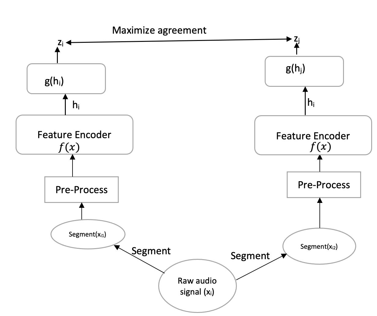
Figure 1: Overall structure of the proposed self-supervised learning for audio representation of environmental sound

3.1 Input Pre-processing

The feature encoder proposed in this work is able to accept two types of inputs. The first type is the normalised waveform similar to the one adopted in [13]. Here, we first segment the raw waveform of length $t$ into two equal parts i.e. each waveform segment has a length $t/2$. The waveform segments’ values are then normalised to zero mean and unit variance. The normalised waveform acts as the first type of input to the feature encoder can accept. The second type of input that can be accepted by the feature encoder is the spectrogram patches. Here, we segment raw audio of time $t$ into two segments each of length $t/2$. From each segment we extract a sequence of 128-dimension log Mel spectrogram features computed using a 25 ms Hamming window with 10 ms stride yielding a spectrogram $X$ of size ${128\times 100t}$. We then randomly select a number of rectangular patches in time from the full Mel spectrogram to act as the input to the feature encoder. Each $x_{i}$ patch has the shape $128\times 100t$ where $t$ is the length of the patch.

3.2 Feature Encoder

For the feature encoder, we use a 1D convolution neural network (CNN). The 1D CNN has been used successfully in other domains such as in fault detection [21] and patient electrocardiogram classification [22]. It was utilised in these domains since it has a low computational complexity and it is able to extract features of dataset without any predetermined transformation. Since the proposed feature encoder can accept both raw waveform and spectrogram as its input, 1D CNN was considered ideal. The main unique architectural design of the 1D CNN is that each CNN layer is equipped to perform both convolution and subsampling [22] [21]( see fig 2). To compute the input of a neuron $k$ at layer $l$, the output maps of the previous layer $l-1$ are convolved with their respective kernels and then summed to obtain $x_{k}^{l}$ the input of neuron $k$ at layer $l$ (eqn 1).

$$x_{k}^{l}=b_{k}^{l}+\sum_{i=1}^{N}Conv1D(w_{ik},s_{i}^{l-1})$$ (1)

where $w_{ik}^{l-1}$ is the weight connecting $i^{th}$ neuron at layer $l-1$ and $k$ neuron in layer $l$. $s_{i}^{l-1}$ is the output of the $i$ neuron at layer $l-1$, $b_{k}^{l}$ is the bias of the $k^{th}$ neuron at layer $l$. To compute the output $s_{k}^{l}$of the $k^{th}$ neuron at layer $l$, $x_{k}^{l}$ processed via a non-linear function $f$ ( eqn 2) then sub-sampling is applied (eqn 3).

$$y_{k}^{l}=f(x_{k}^{l})$$ (2)

$$s_{k}^{l}=Subsampling(y_{k}^{l})$$ (3)

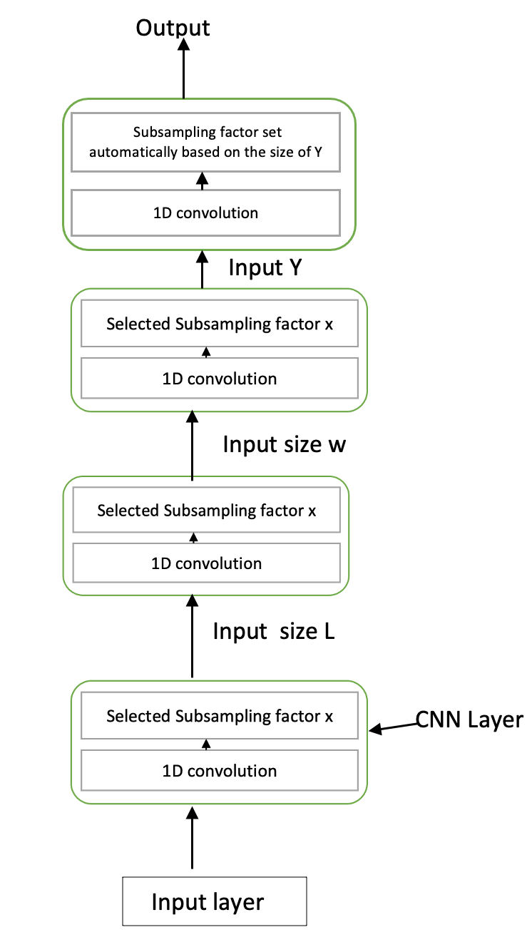
Figure 2: 1D CNN with four CNN layers

The 1D CNN architecture is also adaptive and allows for any number of hidden layers. This is enabled by the fact that the last sub-sampling factor is dynamically set to be equal to the size of its input map.

4 Model Training with normalised waveform as the input

The self-supervised contrastive framework for generating environmental sound representation is based on the idea that two audio waveform segments $x_{i}$ and $x_{j}$ generated from a given waveform $X$ are likely to contain some level of overlapping information. This is based on our analysis of UrbanSound8K [23] dataset where the majority of the waveform visualisation has a repetitive nature hence exhibiting high periodicity ( see fig 3 for some visualisations of selected raw waveforms). During training we seek to learn environmental sound audio representations by setting up a contrastive task $\mathcal{C}$ which requires that a segment $s_{i}$ should be able to identify its sibling from a set of other segments. To compute the loss $\mathcal{L}$, we sample a random mini-batch of $M$ examples of raw waveforms and segment each into two equal parts resulting in $2M$ raw waveforms each of size $t/2$. Each of the $2M$ raw waveforms are then normalised to zero mean and unit variance. The normalised waveforms serve as the input of the feature encoder. The feature encoder generates waveform representation $h$ which is then projected to an MLP network which produces final representation $z$ where contrastive loss is applied. Denoting as $z_{i}$ and $z_{i}^{\prime}$ the two segment representations of audio sounds of the $i^{th}$ audio input, the contrastive loss is defined according to equation 4.

$$\mathcal{L}=\frac{1}{M}\sum_{i=1}^{i=M}L_{i}$$ (4)

and

$$L_{i}=\log\frac{\exp(\nicefrac{{sim(z_{i},z_{i}^{\prime})}}{{\tau}})}{\sum_{k=1}^{i=2M}\mathbb{1}_{[k\neq i]}\exp(\nicefrac{{sim(z_{i},z_{k})}}{{\tau}})}$$ (5)

where $sim(u,v)=\frac{u^{T}v}{||u||||v||}$

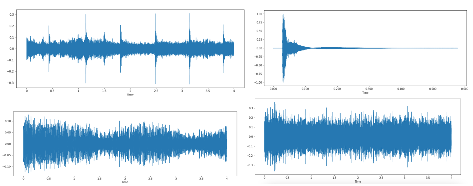
Figure 3: Raw waveform of car horn, gun shot, street music and air conditioner respectively.

5 Model Training with Spectrogram as input

Here, we sample a random mini-batch of $M$ examples of raw waveforms and segment each into two equal parts resulting in $2M$ raw waveforms each of size $t/2$. From each segment we extract a sequence of 128-dimension log Mel spectrogram features as described in section 3.1. From the full Mel spectrogram of a segment, we then randomly select rectangular patches in time. Each patch has a fixed duration of 1.5 s resulting in a rectangular patch of shape $P\in R^{128\times 150}$. The patches are then mapped to 1D vector embedding of size 768 through a trainable non-linear projection( see eqn 6) introduced just before the feature encoder. The embeddings are then projected to the feature encoder and finally to the MLP where contrastive learning is applied according to equation 4 and 5.

$$k=f(W(P_{1}^{T}E+P_{2}^{T}E+\cdots+P_{N}^{T}E))$$ (6)

where $E\in R^{128\times 768}$ and $N$ is the total number of randomly patches selected per Mel spectrogram of a segment and $W\in R^{1\times 150}$ and $f$ is a nonlinear function.

6 Feature Fusion of waveform and spectrogram representation

Here both the normalized raw waveform and the extracted patches of spectrogram are fed into two trained contrastive learners as shown in figure 1. The two feature representations generated by the two contrastive learners are fused using canonical correlation analysis (CCA) [24], [25] into a single global representation. We begin by giving a brief review of key intuition behind CCA. Consider two multivariate random vector ($\textbf{x},\textbf{y})$. The idea behind CCA is to find the basis vectors $\beta$ and $\alpha$ for two sets of variables x and y such that the correlation between the projections of x and y onto the basis vectors $\beta$ and $\alpha$ i.e. $k_{1}=\beta^{T}x$ and $w_{1}=\alpha^{T}x$ are mutually maximized. If $S_{x}=\{x_{1},x_{2},\cdots c_{n}\}$ and $S_{y}=\{y_{1},y_{2},\cdots y_{n}\}$, CCA seeks to define a new direction of $S_{x}$ by choosing a new direction $\beta$ and projecting the vector $S_{x}$ onto that direction i.e $S_{x}\beta=(\langle\beta,x_{1}\rangle,\langle\beta,x_{2}\rangle,\cdots,\langle\beta,x_{n}\rangle)$. Similarly, $S_{y}$ can be projected to a new directions by choosing a direction $\alpha$ i.e. $S_{y}\alpha=(\langle\alpha,y_{1}\rangle,\langle\alpha,y_{2}\rangle,\cdots,\langle\alpha,y_{n}\rangle)$. The first task therefore is to select $\beta$ and $\alpha$ that maximise the correlation between the two vectors according to

$$\sigma=\max_{\alpha,\beta}corr(S_{x}\beta S_{y}\alpha)=\max_{\alpha,\beta}\frac{\langle S_{x}\beta,S_{y}\alpha\rangle}{||S_{x}\beta||||S_{y}\alpha||}$$

Defining the empirical expectation of a function $f(\textbf{x,y})$ as

$$E[f(x,y)]=\frac{1}{m}\sum_{i=1}^{i=m}f(\textbf{x,y})$$

the expression of $\sigma$ can be rewritten as

$$\sigma=\max_{\alpha,\beta}\frac{E[\langle\beta,\textbf{x}\rangle\langle\alpha,\textbf{y}\rangle]}{\sqrt{E[\langle\beta,\textbf{x}\rangle^{2}]E[\langle\alpha,\textbf{y}\rangle]^{2}]}}$$

$$=\max_{\alpha,\beta}\frac{E[\langle\beta,\textbf{x}\rangle\langle\alpha,\textbf{y}\rangle]}{\sqrt{E[\beta^{\prime}\textbf{xx}^{\prime}\beta]E[\alpha^{\prime}\textbf{yy}^{\prime}\alpha)]}}$$

$$=\max_{\alpha,\beta}\frac{\beta^{\prime}E[\textbf{xy}^{\prime}]\alpha^{\prime}}{\sqrt{\beta^{\prime}_{x}E[\textbf{xx}^{\prime}]\beta\alpha^{\prime}E[\textbf{yy}^{\prime}]\alpha)}}$$

Note that the covariance matrix of (x,y) as

$$cov(x,y)=E\left[\begin{bmatrix}\textbf{x}\\ \textbf{y}\\ \end{bmatrix}\begin{bmatrix}\textbf{x}\\ \textbf{y}\\ \end{bmatrix}^{\prime}\right]=\begin{bmatrix}C_{\textbf{xx}}&C_{\textbf{xy}}\\ C_{\textbf{yx}}&C_{\textbf{yy}}\end{bmatrix}$$

$cov(\textbf{x,y})$ matrix is composed of within set covariance $C_{\textbf{xx}}$ and $C_{\textbf{yy}}$ and the between the set covariance $C_{\textbf{xy}}=C_{\textbf{yx}}^{\prime}$ based on this, $\sigma$ can be rewritten as

$$\sigma=\max_{\alpha,\beta}\frac{\beta^{\prime}C_{\textbf{xy}}\alpha^{\prime}}{\sqrt{w^{\prime}_{x}C_{\textbf{xx}}\beta\alpha^{\prime}C_{\textbf{yy}}\alpha^{\prime}}}$$ (7)

therefore canonical correlation is maximised based on the values of the basis vectors $\beta$ and $\alpha$

In this work, Given the two feature vectors $Z$ and $R$ , we exploit CCA to fuse the two features into a single representation that only keeps discriminant information and reduces redundancy between the two representations as much as possible. To fuse the two representations we follow the following steps [25];

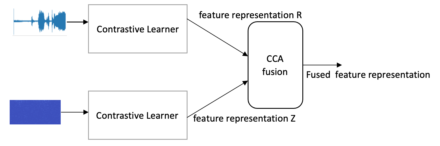
Figure 4: Fusing representation from different input types.

First use the trained contrastive learners to extract two feature vectors representation of the raw waveform and the spectrogram (see fig 4). We then perform the canonical correlation analysis (CCA) between the two representations for fusion as follows;

1. Compute the covariance matrices $S_{rr}$,$S_{zz}$ and $S_{rz}$ representing covariance matrix of $R$, $Z$ and between $Z$ and $R$ respectively.

2. Compute $G1=S_{rr}^{-1/2}S_{rz}S_{zz}^{-1}S_{zr}S_{rr}^{-1/2}$, $G2=S_{zz}^{-1/2}S_{zr}S_{rr}^{-1}S_{rz}S_{zz}^{-1/2}$ and establishing their non-zero eigenvalues $\lambda_{1}^{2}\geq\lambda_{2}^{2}\geq\cdots\geq\lambda_{r}^{2}$ and corresponding orthonormal eigenvectors $u_{i}$ and $v_{i}$ with $1\leq i\leq r$

3. Compute iteratively the canonical projection vectors (CPV) $\alpha_{i}$ and $\beta_{i}$ where $1\leq i\leq r$. $\alpha_{i}$ and $\beta_{i}$ are computed such that they maximise the correlation between the projections $a_{i}=\alpha_{i}^{T}R$ and $b_{i}=\alpha_{i}^{T}Z$. The projections $a_{i}$ and $b_{i}$ are referred to as a pair of canonical variates.

4. Select the first $d$ pair of projections such that $R^{*}=(\alpha_{1}^{T}z,\alpha_{2}^{T}z,\cdots,\alpha_{d}^{T}z)=(\alpha_{1},\alpha_{2},\cdots,\alpha_{d})^{T}z=W_{z}^{T}z$ and $Z^{*}=(\beta_{1}^{T}r,\beta_{2}^{T}r,\cdots,\beta_{d}^{T}r)=(\beta_{1},\beta_{2},\cdots,\beta_{d})^{T}z=W_{r}^{T}r$.

5. Compute feature fusion as $T=X^{*}+Y^{*}$

7 Experimental Setup

7.1 Contrastive Training Details

The 1D CNN was implemented with 4 convolution layers. For the three hidden layers we used 64,32 and 16 neurons respectively. The kernel sizes used were 1,9,15 and 4 for the first, second, third and fourth CNN layers. We also use a sub-sampling value of 4 for the first three layers and the last CNN layer is set to 5 automatically. The output of the last CNN layer is fed into a 2 layer MLP for the final projection of the audio features to the 128-D representations. We use the Adam optimizer for the optimization, batch size of 64, learning rate of 0.001 and training steps of 400. ReLu activation is used in all layers. Further, a dropout is added to the fully connected layer with a probability of 0.5.

7.2 Dataset

We exploited two datasets to evaluate the model proposed in this work. The first dataset is $ESC-50$ [26] which has 50 unique classes of audio data. Each class has 40 audio data with a length of 5 s. The $ESC-50$ dataset is balanced i.e. each class contains 40 audio data. The second dataset is the UrbanSound8K [23] that contains annotated audio sounds collected from the urban setting. It contains 10 classes ( see table 1). The audio clips have varying lengths with the longest being 4 seconds. Further this dataset is class imbalanced i.e. some classes contain instances that are less than 1000. The distribution is shown in table 2.

Table 2: Number of audio per class in UrbanSound8K dataset

Class	Number of instances
Street Music	1000
Siren	929
Gun shot	374
Engine idling	1000
drilling	1000
dog bark	1000
children playing	1000
car horn	429
Air conditioner	1000
Total	8732

7.3 Mini-batch balancing

The UrbanSound8K is unbalanced, therefore training the model with this unbalanced dataset may generate a model that shows weak generalisation ability for the minority classes. To mitigate against this, we adopt the balanced mini-batch training [27]. We allow for an overlap selection of minority samples within the same epoch. Further, we restrict the number of samples from each class in a given mini-batch to be equal to the batch size divided by the number of classes.

7.4 Evaluation objectives

We conducted a number of experiments with a goal to establish if;

1. The proposed method generates environmental audio representation that results in accurate classifications of the environmental sounds.

2. The input type significantly affect the quality of representations generated by the proposed method.

3. Increasing the depth of 1D CNN improves the quality of representations generated by the proposed model.

4. Mini-batch balancing has any effect in boosting the classifications of minority classes.

7.5 What is the quality of audio representation generated by the proposed model

The first experiment is to evaluate the ability of representations generated by the proposed technique to capture the features of the audio dataset. To do this, we set up a classification task by adding a 1 MLP layer of size 10 for the UrbanSound8K and 50 for $ESC-50$ dataset on top of a trained contrastive learner. Our goal is to establish the ability of the representations generated by the learner in classifying the environmental sounds correctly. We evaluate the three possible configurations;

1. When the input to the contrastive learner is normalised raw waveform.

2. When the input to the contrastive learner is the spectrogram patches.

3. When there is fusion of both raw waveform and the spectrogram features.

The results are shown in table 3.

Table 3: Performance of the three configurations proposed in this work.

Technique	ESC-50	UrbanSound8K
Contrastive (raw waveform)	94.42	95.1
Contrastive (spectrogram patches)	94.9	95.43
Contrastive (fusion)	96.2	97.1

From the results in table 3, when raw waveform is the input, the model reports the lowest accuracy as compared to the other two. However, the margin of results between contrastive (raw waveform) and contrastive (spectrogram patches) is marginal, signalling the ability of 1D CNN to capture the features of both untransformed and transformed waveforms well. The fused features between the representations of raw waveform and spectrogram gives superior results demonstrating the need to capture feature representation from both the input types.

8 What is the effect of CNN depth on the quality of representations generated

Here, we experimented with different number of 1D CNN layers in the feature encoder to establish the optimum depth of the 1D CNN model that produces audio representations that capture more accurate features of an audio input. We used a 1D CNN with 4,6,8 and 10 layers. The number of neurons used in each layer is shown in table 4. We mainly use 1,9,15 and 6 as the kernel sizes and sub-sampling factors of 4 and 2.

Table 4: No. of neurons used in a given layer

Layer	Number of Neurons
2	64
3	32
4	16
5	64
6	32
7	16
8	62
9	32
10	16

The results of the experiments are shown in table 5. From the results, there is no definite trend with the varying number of layers. An increase in the depth of the 1D CNN does not offer significant benefit in terms of classification accuracy in all the model configurations. This may point to the ability of the 1D CNN to capture most features even when a shallow depth is used.

Table 5: Effects of varying CNN depth on the performance of the proposed model

	Layers	ESC-50	UrbanSound8K
Contrastive(raw waveform)	4	94.42	95.1
	6	94.67	95.04
	8	94.30	95.12
	10	94.16	95.28
Contrastive(Spectrogram patches)	4	94.9	95.43
	6	95.56	95.49
	8	94.8	95.83
	10	94.94	95.92
Contrastive(fusion)	4	96.2	97.1
	6	96.03	97.41
	8	96.24	97.04
	10	96.76	97.71

8.1 What is the effect of mini-batch balancing on the class prediction

Here we evaluate if mini-balancing improves the classification of the minority classes in the UrbanSound8K. The evaluation uses the contrastive(Spectrogram) model configuration. We first perform training when the mini-batch balancing technique has not been applied during training. The results are shown in the confusion matrix figure 5. From the results the minority classes gunshot and car horn have the lowest classification accuracy of 85% and 89% respectively. This shows that the model does not see enough instances of the two classes to effectively capture their features. Figure 6 shows the confusion results when mini-batch balancing has been applied during training.

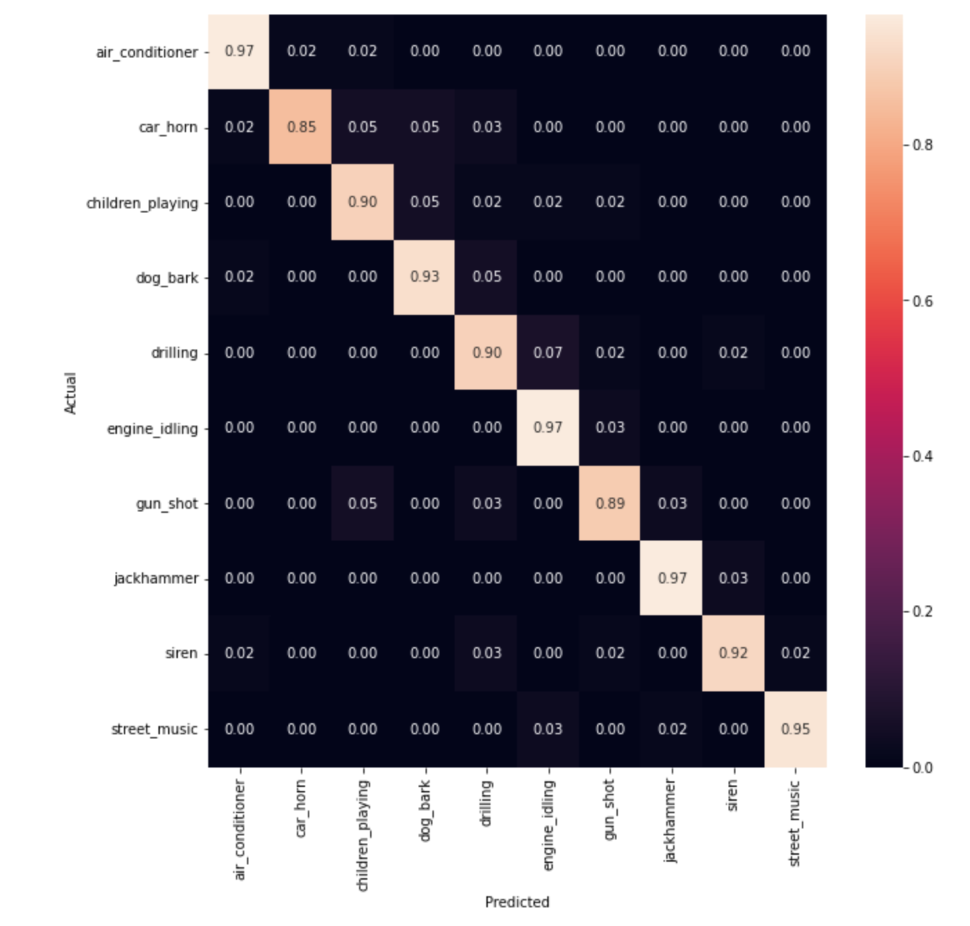
Figure 5: Confusion matrix of evaluation results without mini-batch balancing.

When mini-batch balancing is applied during training, it improves the classification accuracy of car horn and gunshot classes to 91% and 93% respectively, justifying the need for mini-batch balancing during training to boost the number of instances of the minor classes seen by the learner during training hence improving its ability to generalise well for these classes.

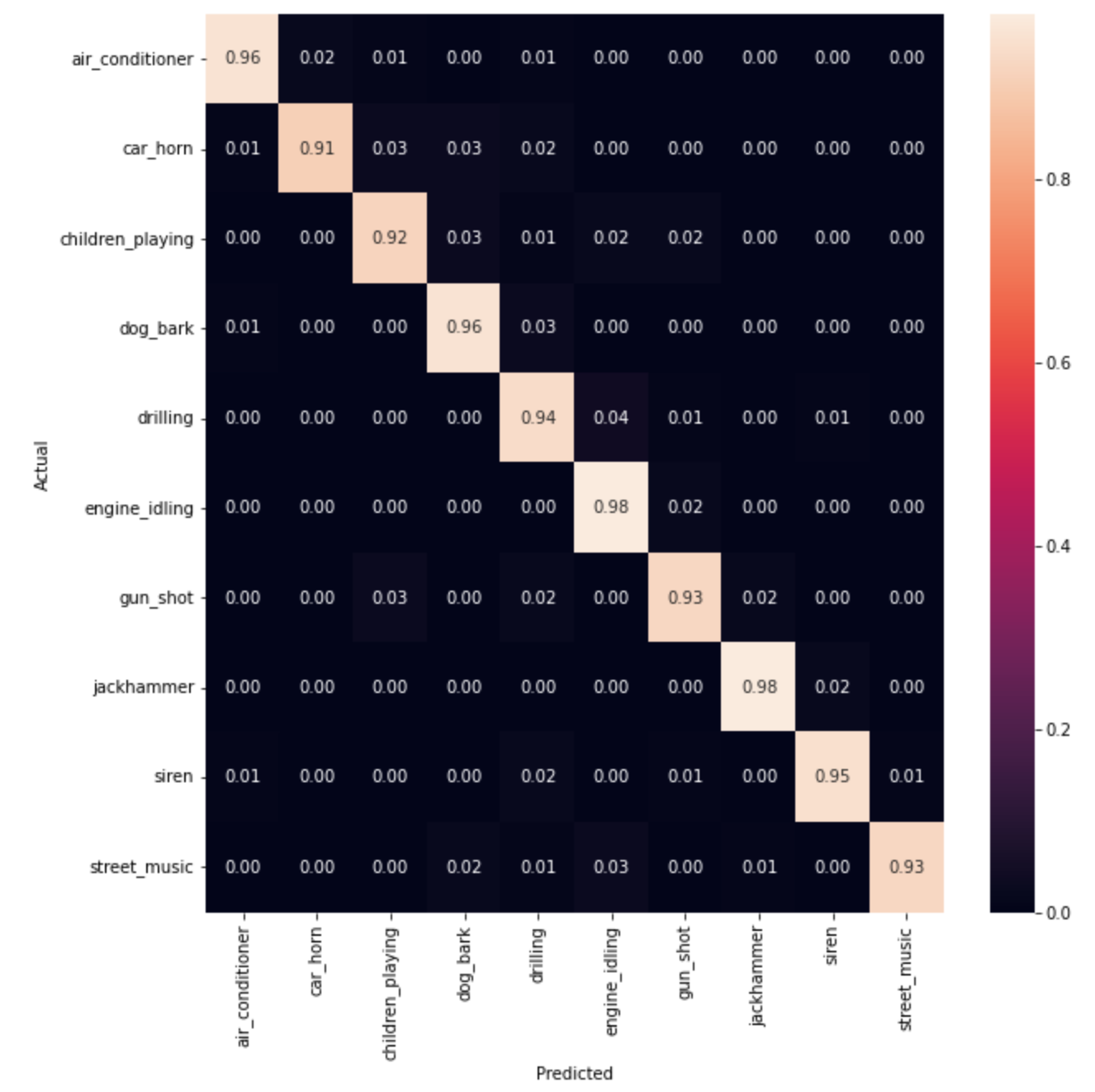
Figure 6: Confusion matrix of evaluation results with mini-batch balancing.

8.2 Comparison to other state of the art tools

Finally, we compared the results of the proposed technique in classifying environmental sounds and the existing state of the art tools for environmental sound classification. We compare the tools on both the ESC-50 and the UrbanSound8K dataset. The results are shown in table 6. On the ESC-50 the three configurations proposed in this work outperforms the existing methods. Contrastive (raw waveform) the least performing technique proposed outperforms the best performing tool TFCNN by a 10% margin. This demonstrates the robustness of the contrastive learning method and the ability of the 1D CNN to capture most of the audio features. On the UrbanSound8K dataset Contrastive (raw waveform) achieves an accuracy of 95.1% which is 2.1% lower than TSCNN the highest performing tool on this dataset. Contrastive(fusion) method outperforms all the existing techniques in both ESC-50 and UrbanSound8K. It records 12.08% increase as compared to the best performing tool TFCNN on the $ESC-50$ dataset. On the UrbanSound8K it achieves an increase of 0.9% as compared to TSCNN is the best performing tool on this dataset.

Table 6: Effects of varying CNN depth on the performance of the proposed model

Tool	ESC-50	UrbanSound8K
Piczak-CNN [8]	65.0%	73.7%
TFCNN [6]	84 .4%	93.1%
Pyramid CNN[7]	81.4%	78.1%
SB_CNN [14]	-	79.0%
SoundNet [16]	74.2%	-
DS-CNN[9]	82.8%	92.2%
TSCNN [28]	-	97.2%
Contrastive (raw waveform)	94.42	95.1
Contrastive (spectrogram patches)	95.3	96.1
Contrastive (fusion)	97.2	98.1

9 Conclusion

This work proposes the use of self-supervised contrastive learning to train a learner which can extract features from the environmental sounds. We exploit a shallow 1D CNN network to extract features of a given audio. We examine the effect of type of input on the quality of representations generated by the learner. Further, we examine the effect of fusing representations from two types of input. The mini-batch balancing is also performed to improve the generalisation of the minority classes by the learner. Overall the proposed technique records a significant improvement in accuracy in the classification task as compared to the existing methods. This demonstrated the robustness of the contrastive learning method and the ability of the 1D CNN to extract the features of waveform.

References

- Elizalde et al. [2022] Benjamin Elizalde, Soham Deshmukh, Mahmoud Al Ismail, and Huaming Wang. CLAP: Learning Audio Concepts From Natural Language Supervision. 2022. URL http://arxiv.org/abs/2206.04769.
- Alías et al. [2016] Francesc Alías, Joan Claudi Socoró, and Xavier Sevillano. A review of physical and perceptual feature extraction techniques for speech, music and environmental sounds. Applied Sciences, 6(5), 2016. ISSN 14545101. doi:10.3390/app6050143.
- Baum et al. [2018] Elizabeth Baum, Mario Harper, Ryan Alicea, and Camilo Ordonez. Sound identification for fire-fighting mobile robots. Proceedings - 2nd IEEE International Conference on Robotic Computing, IRC 2018, 2018-Janua:79–86, 2018. doi:10.1109/IRC.2018.00020.
- Paltz [2005] New Paltz. Regunathan Radhakrishnan , Ajay Divakaran and Paris Smaragdis Mitsubishi Electric Research Labs. Signal Processing, pages 158–161, 2005.
- Youn et al. [2008] Prof M Youn, Prof B H Lee, Prof K Chung, Jia-ching Wang, Hsiao-ping Lee, Jhing-fa Wang, and Cai-bei Lin. The authors would like to acknowledge various forms of help in for Home Automation. Science, 5(1):25–31, 2008.
- Mu et al. [2021] Wenjie Mu, Bo Yin, Xianqing Huang, Jiali Xu, and Zehua Du. Environmental sound classification using temporal-frequency attention based convolutional neural network. Scientific Reports, 11(1):1–14, 2021. ISSN 20452322. doi:10.1038/s41598-021-01045-4.
- Demir et al. [2020] Fatih Demir, Muammer Turkoglu, Muzaffer Aslan, and Abdulkadir Sengur. A new pyramidal concatenated CNN approach for environmental sound classification. Applied Acoustics, 170:1–7, 2020. ISSN 1872910X. doi:10.1016/j.apacoust.2020.107520.
- Piczak [2015a] Karol J Piczak. ENVIRONMENTAL SOUND CLASSIFICATION WITH CONVOLUTIONAL NEURAL NETWORKS Karol J . Piczak Institute of Electronic Systems Warsaw University of Technology. 2015 IEEE 25th International Workshop on Machine Learning for Signal Processing (MLSP), pages 1–6, 2015a.
- Li et al. [2018] Shaobo Li, Yong Yao, Jie Hu, Guokai Liu, Xuemei Yao, and Jianjun Hu. An ensemble stacked convolutional neural network model for environmental event sound recognition, 2018. ISSN 20763417.
- Verma et al. [2020] Vikas Verma, Minh-Thang Luong, Kenji Kawaguchi, Hieu Pham, and Quoc V. Le. Towards Domain-Agnostic Contrastive Learning. 2020. URL http://arxiv.org/abs/2011.04419.
- He et al. [2016] Kaiming He, Xiangyu Zhang, Shaoqing Ren, and Jian Sun. Deep residual learning for image recognition. Proceedings of the IEEE Computer Society Conference on Computer Vision and Pattern Recognition, 2016-Decem:770–778, 2016. ISSN 10636919. doi:10.1109/CVPR.2016.90.
- Clark et al. [2020] Kevin Clark, Minh-Thang Luong, Quoc V. Le, and Christopher D. Manning. ELECTRA: Pre-training Text Encoders as Discriminators Rather Than Generators. pages 1–18, 2020. URL http://arxiv.org/abs/2003.10555.
- Baevski et al. [2020] Alexei Baevski, Henry Zhou, Abdelrahman Mohamed, and Michael Auli. wav2vec 2.0: A framework for self-supervised learning of speech representations. Advances in Neural Information Processing Systems, 2020-Decem(Figure 1):1–19, 2020. ISSN 10495258.
- Salamon and Bello [2017] Justin Salamon and Juan Pablo Bello. Deep Convolutional Neural Networks and Data Augmentation for Environmental Sound Classification. IEEE Signal Processing Letters, 24(3):279–283, 2017. ISSN 10709908. doi:10.1109/LSP.2017.2657381.
- Zhang et al. [2021] Zhichao Zhang, Shugong Xu, Shunqing Zhang, Tianhao Qiao, and Shan Cao. Attention based convolutional recurrent neural network for environmental sound classification. Neurocomputing, 453:896–903, 2021. ISSN 18728286. doi:10.1016/j.neucom.2020.08.069. URL https://doi.org/10.1016/j.neucom.2020.08.069.
- Aytar et al. [2016] Yusuf Aytar, Carl Vondrick, and Antonio Torralba. SoundNet: Learning sound representations from unlabeled video. Advances in Neural Information Processing Systems, (Nips):892–900, 2016. ISSN 10495258.
- Dai et al. [2017] Wei Dai, Chia Dai, Shuhui Qu, Juncheng Li, and Samarjit Das. Very deep convolutional neural networks for raw waveforms. ICASSP, IEEE International Conference on Acoustics, Speech and Signal Processing - Proceedings, pages 421–425, 2017. ISSN 15206149. doi:10.1109/ICASSP.2017.7952190.
- Qian et al. [2021a] Rui Qian, Tianjian Meng, Boqing Gong, Ming Hsuan Yang, Huisheng Wang, Serge Belongie, and Yin Cui. Spatiotemporal Contrastive Video Representation Learning. Proceedings of the IEEE Computer Society Conference on Computer Vision and Pattern Recognition, pages 6960–6970, 2021a. ISSN 10636919. doi:10.1109/CVPR46437.2021.00689.
- Qian et al. [2021b] Rui Qian, Tianjian Meng, Boqing Gong, Ming Hsuan Yang, Huisheng Wang, Serge Belongie, and Yin Cui. Spatiotemporal Contrastive Video Representation Learning. Proceedings of the IEEE Computer Society Conference on Computer Vision and Pattern Recognition, pages 6960–6970, 2021b. ISSN 10636919. doi:10.1109/CVPR46437.2021.00689.
- Jaiswal et al. [2020] Ashish Jaiswal, Ashwin Ramesh Babu, Mohammad Zaki Zadeh, Debapriya Banerjee, and Fillia Makedon. A Survey on Contrastive Self-Supervised Learning. Technologies, 9(1):2, 2020. doi:10.3390/technologies9010002.
- Eren et al. [2019] Levent Eren, Turker Ince, and Serkan Kiranyaz. A Generic Intelligent Bearing Fault Diagnosis System Using Compact Adaptive 1D CNN Classifier. Journal of Signal Processing Systems, 91(2):179–189, 2019. ISSN 19398115. doi:10.1007/s11265-018-1378-3.
- Malik et al. [2022] Junaid Malik, Ozer Can Devecioglu, Serkan Kiranyaz, Turker Ince, and Moncef Gabbouj. Real-Time Patient-Specific ECG Classification by 1D Self-Operational Neural Networks. IEEE Transactions on Biomedical Engineering, 69(5):1788–1801, 2022. ISSN 15582531. doi:10.1109/TBME.2021.3135622.
- Salamon et al. [2014] Justin Salamon, Christopher Jacoby, and Juan Pablo Bello. A dataset and taxonomy for urban sound research. MM 2014 - Proceedings of the 2014 ACM Conference on Multimedia, (1):1041–1044, 2014. doi:10.1145/2647868.2655045.
- Hardoon et al. [2003] David R Hardoon, Sandor Szedmak, and John Shawe-taylor. Canonical correlation analysis ; An methods. Science, 16(12):2639–64, 2003. URL http://www.ncbi.nlm.nih.gov/pubmed/15516276.
- Sun et al. [2005] Quan Sen Sun, Sheng Gen Zeng, Yan Liu, Pheng Ann Heng, and De Shen Xia. A new method of feature fusion and its application in image recognition. Pattern Recognition, 38(12):2437–2448, 2005. ISSN 00313203. doi:10.1016/j.patcog.2004.12.013.
- Piczak [2015b] Karol J. Piczak. ESC: Dataset for environmental sound classification. MM 2015 - Proceedings of the 2015 ACM Multimedia Conference, pages 1015–1018, 2015b. doi:10.1145/2733373.2806390.
- Shimizu et al. [2019] Ryota Shimizu, Kosuke Asako, Hiroki Ojima, Shohei Morinaga, Mototsugu Hamada, and Tadahiro Kuroda. Balanced mini-batch training for imbalanced image data classification with neural network. Proceedings - 2018 1st IEEE International Conference on Artificial Intelligence for Industries, AI4I 2018, pages 27–30, 2019. doi:10.1109/AI4I.2018.8665709.
- Su et al. [2019] Yu Su, Ke Zhang, Jingyu Wang, and Kurosh Madani. Environment sound classification using a two-stream CNN based on decision-level fusion. Sensors (Switzerland), 19(7), apr 2019. ISSN 14248220. doi:10.3390/s19071733.