Core-collapse Supernovae in the Dark Energy Survey: Luminosity Functions and Host Galaxy Demographics

Abstract

We present the luminosity functions and host galaxy properties of the Dark Energy Survey (DES) core-collapse supernova (CCSN) sample, consisting of 69 Type II and 50 Type Ibc spectroscopically and photometrically-confirmed supernovae over a redshift range $0.045<z<0.25$. We fit the observed DES $griz$ CCSN light-curves and K-correct to produce rest-frame $R$-band light curves. We compare the sample with lower-redshift CCSN samples from Zwicky Transient Facility (ZTF) and Lick Observatory Supernova Search (LOSS). Comparing luminosity functions, the DES and ZTF samples of SNe II are brighter than that of LOSS with significances of 3.0$\sigma$ and 2.5$\sigma$ respectively. While this difference could be caused by redshift evolution in the luminosity function, simpler explanations such as differing levels of host extinction remain a possibility. We find that the host galaxies of SNe II in DES are on average bluer than in ZTF, despite having consistent stellar mass distributions. We consider a number of possibilities to explain this – including galaxy evolution with redshift, selection biases in either the DES or ZTF samples, and systematic differences due to the different photometric bands available – but find that none can easily reconcile the differences in host colour between the two samples and thus its cause remains uncertain.

1 Introduction

Core-collapse supernovae (CCSNe) are among the most complex and diverse astrophysical events, demonstrating a wide range of spectroscopic and photometric properties (Filippenko, 1997; Gal-Yam, 2017; Modjaz et al., 2019). Type II SNe show hydrogen features in their spectra due to the outer hydrogen envelope of the progenitor star, while stripped envelope SNe (i.e., SNe Ib, Ic, IIb) present different features depending on the degree to which the outer hydrogen and helium envelopes have been stripped away by processes such as stellar winds (e.g., Woosley et al., 1993) and binary interaction (e.g., Nomoto et al., 1995). While it is generally understood that CCSNe result from the cessation of fusion in the cores of massive stars after the formation of iron leading to the core collapsing, there is a great deal that remains uncertain about the exact mechanisms of this process. Studying the properties of populations of CCSNe can help constrain our knowledge of the processes involved in the explosion (Li et al., 2011; Richardson et al., 2014).

The most straightforward population diagnostic is the luminosity function, the distribution of peak luminosities observed across the SN population. An accurate knowledge of the luminosity function is important in simulating CCSN explosions to ensure they exhibit the range of properties of the observed population. Luminosity functions are also important when simulating sky surveys to ensure simulated SNe are created with realistic properties. Simulations of this nature are used for a number of applications, for example calculating SN rates (e.g., Bazin et al., 2009; Graur et al., 2017a; Frohmaier et al., 2021), optimising observing strategies and preparing for upcoming surveys (e.g., Jones et al., 2017; Villar et al., 2018) and modelling the contamination of CCSNe in cosmological samples of SNe Ia (e.g., Vincenzi et al., 2019; Vincenzi et al., 2021b).

The host galaxies of SNe provide further demographic information about their properties and sample the stellar populations from which the progenitor star is drawn. CCSNe are generally found across a wide variety of star-forming host galaxy environments (e.g. Anderson et al., 2010; Graur et al., 2017b), while the most luminous transients (e.g., superluminous supernovae, broad line SNe Ic, see e.g. Angus et al., 2016; Perley et al., 2016; Modjaz et al., 2020) and rapidly-evolving transients (RETs, Wiseman et al., 2020b) are typically found in low mass, low metallicity and/or strongly star-forming environments. SNe Ib/c have also been shown to more closely trace underlying star formation in their host galaxies than SNe II (e.g., Anderson & James, 2009; Galbany et al., 2018).

Several studies have examined CCSNe luminosity functions, primarily in the local universe. For example, Li et al. (2011, hereafter L11) produced luminosity functions for all SNe in the Lick Observatory Supernova Search (LOSS; Li, 2000), including 105 CCSNe, and Richardson et al. (2014) presented luminosity functions based on data from the Asiago Supernova Catalogue (Barbon et al., 1989) supplemented by further SNe from other studies. Here, we measure luminosity functions based on SNe detected by the Dark Energy Survey (DES) Supernova Program (DES-SN, Bernstein et al., 2012). DES-SN is a deep, untargeted, five-season rolling SN search survey over 27 deg² of sky. This leads to a higher redshift sample than presented in previous work (Smith et al., 2020b), providing an opportunity to study any redshift evolution in the CCSN luminosity function and the effect of any evolution in the SN host galaxy populations (e.g. Elbaz et al., 2011): such an evolution may in turn lead to an evolution in the CCSN population. The Zwicky Transient Facility’s (ZTF) Bright Transient Survey (Perley et al., 2020) provides an additional sample of CCSNe which lie in a redshift range between that of DES and LOSS. We also include this sample in our analysis to allow for further investigation of any redshift evolution.

In this paper, we present luminosity functions and host galaxy properties of CCSNe in DES, and compare these to samples from LOSS and ZTF. In Section 2, we detail these three samples and describe the selection of objects suitable for inclusion in a luminosity function. Section 3 describes the method used to construct luminosity functions for both DES and ZTF, and presents the luminosity functions themselves. In Section 4 we discuss the host galaxy demographics of the samples and the correlations between different host properties and peak SN luminosity. We discuss our results in Section 5 and conclude in Section 6. Throughout, we assume a flat $\Lambda$CDM cosmology with $\Omega_{M}=0.3$ and H${}_{0}=70$ km s^-1 Mpc^-1, and correct external samples to this cosmological model as required. All photometry has been corrected for the effects of Milky Way extinction using dust maps presented in Schlegel et al. (1998) and re-calibrated in Schlafly & Finkbeiner (2011), assuming $R_{V}=3.1$. All quoted magnitudes are in the AB system (Oke & Gunn, 1983).

2 Core-collapse Supernova Samples

We begin by presenting the different CCSN samples we have used for this analysis, detailing the selection criteria applied to the DES and ZTF samples and how we use the data presented in L11. We do not compare with the luminosity functions presented in Richardson et al. (2014). This is because the sample presented is from a wide variety of different instruments and surveys which makes it very difficult to correct for Malmquist bias based on the limiting magnitude of each survey as we do in this work (see Section 3.1). Drout et al. (2011) presents a collection of 25 SNe Ibc and includes peak absolute magnitudes, however, all of these objects are brighter than -17.5, which suggests that only the most intrinsically luminous objects are included. As a result, this sample is not included in our comparisons. A sample of CCSNe is available from SDSS-II (e.g., Taylor et al., 2014), however, peak luminosities and Malmquist bias corrections are not available for these objects to allow for a comparison. Finally, Arcavi et al. (2012) and Kiewe et al. (2012) present SNe II and IIn, respectively, from the Caltech Core-Collapse Project (Gal-Yam et al., 2007, CCCP). However, these samples combined contain relatively few objects with only 12 that have estimated peak absolute magnitudes; a further 9 have absolute magnitudes but of the plateau phase of a SN II rather than peak and 5 have only lower limits for the peak. As a result, we do not compare to this sample in this analysis.

Throughout this analysis, we treat CCSNe as two general classes rather than subdividing further. This is to ensure sufficient numbers of SNe in each class, and to acknowledge the uncertainties in the photometric SN classification that we use in the DES-SN sample. We refer to Type II SNe to include all hydrogen-rich SNe and Type Ibc SNe to include all hydrogen-poor/stripped-envelope SNe. Although SNe IIb, such as the very luminous SN IIb DES14X2fna in the DES-SN sample (Grayling et al., 2021), do show hydrogen features at early times, they also have a partially stripped outer hydrogen envelope and are included with SNe Ibc for this analysis. Table 1 contains summary information for each sample.

Table 1: Sample sizes for our luminosity functions after applying selection criteria.

Survey	Total Sample Size		Sample After Quality Cuts		Sample After Redshift and Magnitude Cuts
	SNe II	SNe Ibc	SNe II	SNe Ibc	SNe II	SNe Ibc
DES (spectroscopically confirmed CCSNe)	52	18	33	13	31	11
DES (photometric CCSNe with host spec-z)	–	–	56	42	38	39
LOSS	69	36	–	–	37	21
ZTF	349	162	214	105	174	89

2.1 The DES core collapse supernova sample

The DES-SN CCSN sample contains three categories of objects: those with a spectroscopic confirmation, those with a spectroscopic redshift of the host galaxy, and those with photometric redshift information for the host galaxy. We discuss each of these in turn.

2.1.1 Spectroscopically confirmed CCSNe

The DES-SN CCSN sample has 70 spectroscopically-confirmed CCSNe between redshifts $0.045<z<0.33$. These were obtained over a variety of telescopes and instruments during the course of the DES survey (Smith et al., 2020a).

We apply the following selection criteria to ensure that the light curve can be analysed to measure the peak SN brightnesses required for the luminosity function:

• Each SN must have photometric coverage before and after maximum to ensure an accurate interpolation of the peak luminosity.

• Each object must have a well-constrained explosion epoch inferred either from the date of last non-detection of the SN, or from spectral template matching using the Supernova Identification code (snid; Blondin & Tonry, 2007) following the prescriptions of Gutiérrez et al. (2017). An explosion epoch is required to select an appropriate model spectral energy distribution (SED) at each epoch for the K-correction of observed photometry to the rest-frame, as the SED models we use are defined with respect to explosion. For objects with pre-explosion non-detections, we assume an explosion epoch halfway between the last non-detection and the first detection.

• Each object must have at least 9 detections which are deemed real by a supervised machined learning classifier (see Goldstein et al., 2015, for details of the classifier). A limit of 9 is selected to maximise both the sample size and photometric coverage, as overall this cut eliminates only 4 objects with the next object only having 6 detections deemed real by the classifier.

This selection leaves 46 spectroscopically-confirmed CCSNe in DES. Of these, 33 are spectroscopically hydrogen-rich (Type II) and 13 hydrogen-poor/stripped-envelope (Type Ibc).

2.1.2 Photometric CCSNe with host spec-z

DES also detected a much larger number of transients which have no spectroscopic confirmation. We first investigate transients which have a spectroscopic measurement of the SN host galaxy redshift (spec-z); for example, from the OzDES survey (Yuan et al., 2015; Childress et al., 2017; Lidman et al., 2020) or external redshift catalogues - Vincenzi et al. (2021b) presents details of the different host galaxy redshift sources using galaxy associations from Wiseman et al. (2020a). To this sample, we apply a number of cuts to select objects that:

• were detected in at least nine epochs based on the classifier detailed in Goldstein et al. (2015) to ensure good photometric coverage, matching the cut applied to spectroscopically confirmed sample in Section 2.1.1.

• have an assigned host galaxy with a spectroscopic redshift less than 0.3 (as an initial redshift cut).

• were single-season transients, removing some obvious AGN.

These cuts gave a total of 1609 transients. We remove all spectroscopically-confirmed objects that are not CCSNe (e.g., SNe Ia, AGN) and remove the remaining AGN using the classifier discussed in Section 2.2.3 of Wiseman et al. (2020b). We next remove SNe Ia from the sample employing the photometric SN classifier SuperNNova (Möller & de Boissière, 2019), using the trained model discussed in Vincenzi et al. (2021a). We follow Wiseman et al. (2021), Möller et al. (2022) and Vincenzi et al. (2021a) in removing all objects with a probability of being a SN Ia ($P_{\textrm{Ia}}$) of greater than 0.5. For the remaining objects, we apply the same quality cuts in terms of requiring coverage pre- and post-peak and a well-constrained explosion date as in Section 2.1.1 and visually inspect the photometry of the remaining objects to ensure they are consistent with a CCSN; 51 objects are excluded as they are active in several observing seasons and do not resemble SNe, while 1 is excluded as it lacks any $r$-band data. We then classify remaining objects as SNe II or SNe Ibc using the light curve template fitter pSNid (Sako et al., 2011) – 8 SNe are excluded as they are either classified as SNe Ia by pSNid or are consistent with both SNe II and Ibc. This leaves a sample of 98 photometrically-confirmed CCSNe from DES, of which 56 are SNe II and 42 SNe Ibc; combined with spectroscopically-confirmed objects, the total DES CCSN sample with spectroscopic redshifts has 89 SNe II and 55 SNe Ibc. The requirement for constraint of peak luminosity means that the quality cuts we apply are relatively strict, making this sample smaller than might be used for other purposes such as rate calculations.

To assess the suitability of pSNid for these purposes, we evaluate its performance for the full sample of 70 spectroscopically-confirmed SNe in DES; we obtain an estimated pSNid class for 69 of these. For SNe II, there are 8 misclassifications out of 51 - 6 are classified as SNe Ia and 2 as SNe Ibc by pSNid. For SNe Ibc, there are 2 misclassifications out of 18 objects, with one misclassified as a SN Ia and one as a SN II. This gives accuracy for these classes of 84 and 89 per cent respectively and an overall accuracy of 86 per cent. We opt to use SuperNNova to remove SNe Ia and then pSNid to separate SNe II from SNe Ibc, rather than simply using pSNid for all SNe, as SuperNNova has been shown to have very high performance upwards of 98 when separating SNe Ia from non-SNe Ia (Möller & de Boissière, 2019; Vincenzi et al., 2021a). Out of all DES transient candidates, of all objects classified as SNe Ia by SuperNNova around 5 per cent are classified as CCSNe rather than SNe Ia by pSNid. The good level of agreement between these classifiers is reassuring, but we favour SuperNNova due to its high performance. It is not possible to use SuperNNova for both tasks as a suitable SuperNNova model for multi-class classification trained on DES-like light curves is not currently available.

It should be noted that we do not apply a confidence threshold based on chi-squared ($\chi^{2}$) - for example, if the SN II template in pSNid is a much better fit to a given SN than either the SN Ia or Ibc templates, it was classified as a SN II regardless of the SN II template $\chi^{2}$ value when fitting the light curve. Given all the checks and cuts we apply to remove SNe Ia and other types of transients prior to using pSNid, we can be confident that all remaining objects are CCSNe and are therefore justified in not using a $\chi^{2}$ cut. Nevertheless, as a check, we analyse the properties of the sample excluding the 20 objects with the worst $\chi^{2}$ values and find that this does not impact the trends we observe.

2.1.3 Photometric CCSNe with host photo-z

Beyond the sample of CCSNe with spectroscopic host redshifts, there are a number of CCSNe in DES with no spectroscopic information, for example because the host was too faint to take a reliable spectrum. While we cannot directly include these objects in our luminosity function, it is important to understand any selection effects that arise from excluding these objects from the sample.

Photometric redshifts (photo-zs) have been produced for three of the ten DES-SN fields from coadded photometry as outlined in Hartley et al. (2022), based on the photometric redshift fitting code EAzY (Brammer et al., 2008). To produce a sample of DES CCSNe without spectroscopic host redshifts, we take all real transient candidates in the full DES-SN sample, select those located in hosts with photometric redshifts, and remove known AGN and other transient types such as variable stars using existing catalogues. We use SuperNNova to remove all likely SNe Ia using a model trained without spectroscopic redshift information - this cut leaves 45 objects (again, using $P_{\textrm{Ia}}>0.5$). Finally, we visually inspect each light curve to remove other types of transient that are clearly not SN-like in nature (e.g., AGN) and apply the same quality cuts as in Sections 2.1.1 and 2.1.2, leaving 25 CCSNe.

As we apply redshift cuts in this analysis and there are large uncertainties in photometric redshifts, the exact size of this sample is not fixed but typically varies between 3 and 8 – this is discussed in detail in Appendix A. In brief, this analysis suggests that we obtain spectroscopic host redshifts for $\sim 75-90$ per cent of CCSNe observed by DES. This sample of objects with photometric redshifts is used only for selection efficiency checks.

2.2 The ZTF Bright Transient Survey

Perley et al. (2020) presents a public catalogue of transients from the ZTF Bright Transient Survey with spectroscopic classifications. Excluding SNe Ia and super-luminous SNe, this sample consists of 511 CCSNe. For all of these objects, we gather publicly-available $g$ and $r$-band photometry from the Lasair transient broker (Smith et al., 2019). We apply the same cuts as for the DES sample, only including objects with photometric coverage both pre and post-peak in both bands and with a well-constrained explosion date. This leaves a sample of 319 CCSNe from ZTF: 214 SNe II and 105 SNe Ibc, applying our broad classifications as described earlier.

2.3 LOSS

The Lick Observatory Supernova Search (LOSS; Li, 2000) was a galaxy-targeted SN survey that monitored approximately 5000 nearby galaxies for transients using the Katman Automatic Imaging Telescope (KAIT). Luminosity functions of different SN sub-types from LOSS were presented in L11, and we re-categorise these into our broader classifications. Note that L11 includes SNe IIb with SNe II rather than SNe Ibc, hence the LOSS luminosity functions presented here will differ slightly from L11. With this classification scheme the LOSS sample contains 105 CCSNe: 69 SNe II and 36 SNe Ibc. It should be noted that Shivvers et al. (2017) revisits the classification of the LOSS sample, with some object classes modified from L11. However, because we are using broad labels of SNe II and Ibc, in all cases the new class falls into the same category as the original. In Shivvers et al. (2017), there are a small number of SNe which show hydrogen lines with only a single spectrum which are presented as having an uncertain class of either SN II or SN IIb. We class these objects as SNe II as robust classification of a SN IIb requires multiple spectra showing the transition from hydrogen to helium, although changing this has little impact on our results.

Note that for this analysis we correct the LOSS absolute magnitudes presented in L11 from H${}_{0}=73$ km s^-1 Mpc^-1 to H${}_{0}=70$ km s^-1 Mpc^-1 and also convert from Vega to AB magnitudes using conversions from Blanton & Roweis (2007). This is done to ensure consistency with DES and ZTF.

2.4 Host galaxy properties

We also assign every SN across the three samples to a host galaxy, and estimate the physical properties of those hosts. We use DES host galaxy associations and $griz$ photometry from Wiseman et al. (2020a). We perform galaxy SED fits based on the SED models produced by the spectral evolution code PÉGASE.2 (Fioc & Rocca-Volmerange, 1997, 2019) following the procedure as outlined in Smith et al. (2020b) and Kelsey et al. (2020), assuming a Chabrier initial mass function (Chabrier, 2003). This provides us with host galaxy stellar masses, star formation rates (SFRs) and rest-frame colours. These fits require an input redshift: for the sample with photometric redshifts, the larger redshift uncertainties must be accounted for. We calculate distributions of host properties for this sample which factor in redshift uncertainty using a method outlined in Appendix A.

For LOSS, several choices for stellar masses are available. Host galaxy stellar masses are presented in L11 using $K$ and $B$-band mass-to-luminosity ratios, and Graur et al. (2017a) presents stellar mass and SFR values for LOSS hosts from Sloan Digital Sky Survey (SDSS, Blanton et al., 2017) spectroscopy. In addition, the majority of LOSS hosts have stellar mass and SFRs calculated in the literature using a variety of different methods, including using near-infrared and far-ultraviolet flux (Leroy et al., 2019; Karachentseva et al., 2020). However, for consistency across our samples, we obtain $ugriz$ photometry for the hosts from SDSS and follow the same SED-fitting procedure described above. Each SN in LOSS is already matched to a host in Table 4 of Leaman et al. (2011), which we match to a corresponding SDSS galaxy.

Out of 58 LOSS CCSNe in our sample, 30 fall in the SDSS footprint and we are able to match to an SDSS host for 26 of these. To assess the quality of our method, we compare the stellar mass and SFR values calculated from SED fits to previously published literature values (see Appendix B). We find that our inferred stellar masses from SED fitting are consistent with other methods although there is unsurprising scatter in the SFR values derived from SED fits that are known to be difficult to measure using only $ugriz$ data (Childress et al., 2013). As rest-frame $U-R$ colour correlates with morphology and traces star formation (Lintott et al., 2008; Trayford et al., 2016), we instead use rest-frame $U-R$ colour as a proxy for star-formation. We opt to use $U-R$ rather than SFR because it is more directly linked to the observed photometry and is not dependent on the star formation history (SFH) model used in the SED fits. By contrast, the SFR is estimated based on the average SFR over the 250 Myr prior to the best-fit timestep in the SFH (see section 2.2.2 of Smith et al. 2020). It is thus dependent on the choice of that SFH (and sensitive to other assumptions that we make) and is not directly linked to any observable. The $U-R$ colour is directly linked to the observed colours, modulo a $k$-correction (for which the best-fit SED is used). We also find that $U-R$ correlates well with our inferred specific star formation rate (sSFR) values.

For ZTF, we again search for host $ugriz$ photometry in SDSS, using a broad search radius of 50″ radius around the SN position, matching to the closest galaxy and then visually confirming the matches. Out of the 263 CCSNe in our ZTF sample, 212 objects lie within the SDSS footprint and we are able to match 203 of these to an SDSS galaxy.

3 Core collapse SN luminosity functions

We construct luminosity functions for the DES and ZTF samples using the following procedure:

1. We interpolate the observed photometry to obtain simultaneous observations in all photometric bands ($griz$ in the case of DES, $gr$ for ZTF) using Gaussian Processes (GP; Rasmussen & Williams 2005). We use the python package george (Ambikasaran et al., 2015), following the process outlined in Angus et al. (2019). Each photometric band is interpolated separately.

2. We K-correct this interpolated observed photometry to the rest-frame, using SED models for SNe II from Dessart et al. (2013a) and for SNe Ibc from Levan et al. (2005). At each epoch with observations, we interpolate the time series SED to obtain a model SN SED. We then warp the model SED to colour-match it to our GP-interpolated photometry in all bands and use this spectrum for the K-correction.

3. This K-corrected rest-frame photometry is then again interpolated using GPs in order to estimate the peak luminosity of each object as well as its corresponding uncertainty.

We make an additional selection on peak absolute magnitude and redshift for each survey to produce the luminosity functions. The absolute magnitude limit of our combined sample is set by DES as it is the highest redshift survey and thus shallowest in terms of absolute magnitude: we exclude objects with a peak absolute magnitude fainter than $-16$ mag in $R$-band. We also exclude objects brighter than $-19.5$ mag in $R$-band to ensure a like-for-like comparison between the samples as these are only present in ZTF.

We make a redshift selection in the DES sample of $z<0.25$ to obtain a volume-limited sample above our absolute magnitude limit, and similarly use a redshift selection for the ZTF sample of $z<0.06$. This means that our ZTF sample does not overlap in redshift with the DES sample. This leaves 69 SNe II and 58 SNe Ibc in DES, 37 SNe II and 21 SNe Ibc in LOSS, and 177 SNe II and 89 SNe Ibc in ZTF, as detailed in Table 1.

Fig. 1 shows our final samples, including those objects removed by this selection. As shown in Fig. 1, Malmquist bias (i.e. bias towards more luminous objects at higher redshifts) is seen in our samples. The ZTF sample in particular shows a strong trend towards more luminous supernovae at higher redshift - the redshift cut at 0.25 and greater depth of DES means that it is less affected by this, while the local nature of LOSS means that this sample has good completeness over the absolute magnitude range we are studying.

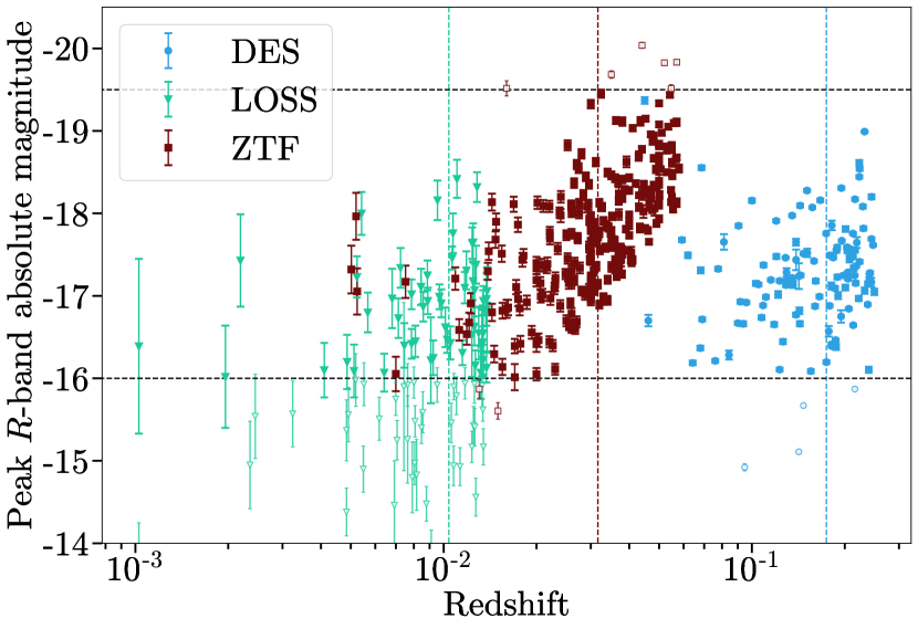
Figure 1: Peak rest-frame CCSN $R$-band absolute magnitude, corrected for Milky Way extinction, plotted against redshift for the DES, LOSS and ZTF CCSN samples. Horizontal dashed lines indicate the median redshift of each SN sample, while vertical dashed lines represent the bounds of the absolute magnitude selection cut we apply. Closed symbols denote SNe included in the final samples and open circles are SNe excluded by the cut.

3.1 Correcting for Malmquist Bias

We correct for Malmquist bias using a simple $V_{\text{max}}$ correction (Schmidt, 1968). This weights fainter objects, which would not be detected (or followed up) over the full survey volume, higher in the luminosity function calculation. For a volume-limited sample with an upper redshift limit $z_{\text{survey}}$, each SN has an upper redshift limit $z_{\text{max}}$, beyond which the object would fall below the detection limit of the survey. We calculate the weight $w$ each object makes to the luminosity function according to

$$w=\begin{cases}\Big{(}\frac{d_{c}(z_{\text{survey}})}{d_{c}(z_{\text{max}})}\Big{)}^{3}&\text{if }z_{\text{max}}<z_{\text{survey}}\\ 1&\text{otherwise}\end{cases}$$ (1)

where $d_{c}$ is the comoving distance. Thus, an intrinsically luminous SN that could have been detected over the full survey volume is given a weight of 1, while a fainter SN is assigned an increased weight.

This approach assumes that each survey has a magnitude limit above which it is complete. For the DES sample we use limits of $m=23.5$ and $m=24.5$ for the shallow and deep fields respectively (Kessler et al., 2015). In reality, completeness in SN surveys is more complex than a simple cut-off, and thus this assumption introduces some uncertainty in the analysis; however, we find that altering these limits within $\pm 0.5$ mag has no significant effect on the luminosity distributions.

For ZTF we consider the 97, 93 and 75 per cent spectroscopic completeness limits of $18$, $18.5$ and $19$ mag respectively (Perley et al., 2020). In brief, we find that we obtain consistent luminosity functions with a limit of either 18.5 or 19 mag and that a limit of 18 mag causes the sample to miss fainter supernovae (see Appendix C). As a result, we use 19 mag as the magnitude limit in this analysis to maximise the sample size.

Finally, we experimented with using the $V_{\mathrm{max}}$ correction for the LOSS sample. However, as expected we found that the sample is complete in the absolute magnitude range we are studying.

We now form the luminosity functions for the three SN samples. We incorporate the weighting (equation 1) into our cumulative distributions using

$$C(M_{n})=\frac{\sum_{i=1}^{n}w_{i}}{\sum_{i=1}^{N}w_{i}},$$ (2)

where $C(M_{n})$ is the cumulative density up to absolute magnitude $M$, $n$ is the index position of in the sorted distribution of $M$ values, $i$ is the index of each supernova and $N$ is the total number of objects. In this section we use the two-sample Kolmogorov–Smirnov (KS) test to compare different luminosity functions – this weighted cumulative distribution is incorporated into all KS tests in this section.

3.2 CCSN luminosity functions

The left two panels of Fig. 2 shows the SN II luminosity functions. Histogram uncertainties in the upper panel represent the expected uncertainties from Poisson statistics and are derived from confidence limits presented in Gehrels (1986), while the cumulative density function (CDF) uncertainties in the lower panel represent the statistical uncertainties in the individual measurement and are estimated from a Monte Carlo (MC) approach described as follows:

• The measured values of peak absolute magnitude and their uncertainties are used as the mean and standard deviations of a Gaussian distribution.

• 1000 randomised CDFs are generated using the Gaussian distribution of each data point.

• The mean and standard deviation of the CDFs at each value are calculated – these are the values and uncertainties plotted.

Uncertainties here will depend on both the uncertainty on the luminosity of each SN and also on the sample size, as for a smaller sample changing an individual measurement will have a larger effect on the CDF. As can be seen, LOSS overall has a larger uncertainty in the CDF than DES in this figure. This is because DES photometry has lower uncertainties than LOSS photometry, meaning that the Gaussian distributions of each point are narrower.

Table 2 shows the results of two-sample KS tests between the different samples, with the $p$-values converted to a significance in $\sigma$. The DES sample overall appears brighter than both LOSS and ZTF, with significances of 3.0$\sigma$ and 1.8$\sigma$ respectively. The ZTF sample is also brighter than LOSS at a significance level of 2.5$\sigma$.

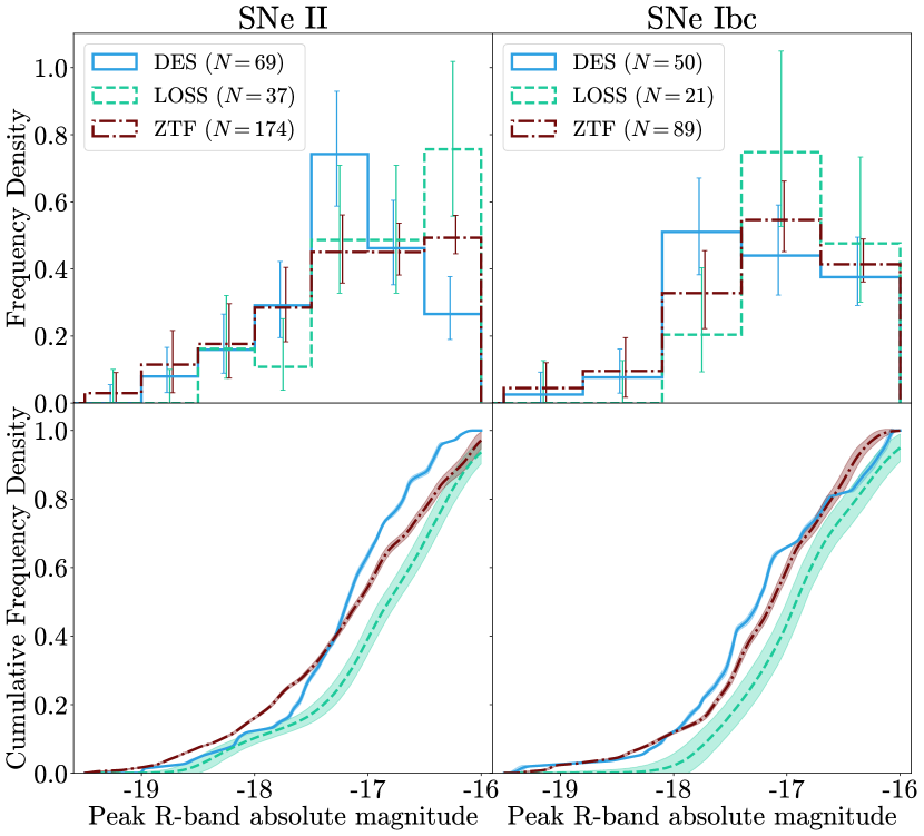
Figure 2: SNe II and Ibc $R$-band luminosity functions for the DES, LOSS and ZTF samples. Each event has been weighted by equation 1 ($V_{\text{max}}$ correction). Histogram uncertainties are from the Poisson distribution confidence limits of Gehrels (1986), while CDF uncertainties are derived from a Monte Carlo approach based on the measurement uncertainty of each value.

Table 2: Two-sample KS tests between the SN II and SN Ibc luminosity functions.

Survey 1	Survey 2	KS test significance
		SNe II	SNe Ibc
DES	LOSS	3.0$\sigma$	1.9$\sigma$
DES	ZTF	1.8$\sigma$	1.1$\sigma$
LOSS	ZTF	2.5$\sigma$	1.8$\sigma$

The right two panels of Fig. 2 shows the luminosity function of SNe Ibc in DES, ZTF and LOSS. DES appears slightly more luminous than both LOSS and ZTF although at low significance levels of 1.9$\sigma$ and 1.1$\sigma$.

3.3 Parameterised luminosity functions

In order to allow these luminosity functions to be used in simulations going forward, we fit a number of different distributions to the histograms presented in Section 3.2. We do this for our newly derived DES and ZTF luminosity functions; LOSS luminosity functions are already presented in L11. These fits are only possible where the distributions peak above $-16$ and begin to decline again as otherwise we cannot constrain the location of the peak of the luminosity function. For SNe II in ZTF, the distribution does not obviously begin to decline above $-16$ which makes this difficult. As a result, for this fit we include two extra SNe which have a peak $R$-band magnitude below $-16$ which allows the peak of the distribution to be constrained. This fit is included for completeness, but we emphasise that the results for SNe II in ZTF should be considered with the strong caveat that these two extra objects have significant weight in determining the location of the peak of the distribution.

We consider both Gaussian and Lorentzian fits to the luminosity functions. We also consider skewed Gaussian distributions but find we are not able to constrain the skewness parameter $\gamma$ with the available data. The parameter values for these fits are shown in Table 3. The exact parameter values for the distributions are sensitive to the binning of the histogram. The values shown in this table are based on the bin edges presented in Fig. 2, from $-19.5$ to $-16$ in steps of 0.5 for SNe II and 0.7 for SNe Ibc. For these fits, we use the mean of the absolute magnitudes in each bin for the x-coordinates. In this table, we present the uncertainty in each parameter when fitting to distributions with these bins (fit error). To take into account the how varying the binning will affect the parameter values, we also present a binning error; this is defined as the standard deviation of the parameter values measured when considering all possible bin widths from 0.10 to 1.0 in steps of 0.01.

To assess the quality of each fit, we also present reduced $\chi^{2}$ values. These are calculated assuming a $\sqrt{N}$ uncertainty in the histogram, rather than the uncertainties based on Gehrels (1986) presented in Fig. 2, in order to provide symmetric uncertainties for the fitting process. For SNe II in DES, a Gaussian distribution provides a reasonable fit although is too broad around the peak and underestimates the number of brighter SNe. A Lorentzian distribution better fits the sharp peak and brighter tail of the luminosity function. For SNe Ibc in DES, both distributions provide similar fits although the Gaussian has a lower reduced $\chi^{2}$. In contrast, for SNe II in ZTF a Gaussian better represents the luminosity function and a Lorentzian overestimates the number of brighter SNe. As for SNe Ibc in ZTF, a Gaussian has a lower reduced $\chi^{2}$ and better represents the luminosity function around peak although again underestimates the number of SNe in the brighter tail.

Table 3: Reduced $\chi^{2}$ values and parameter values for different model fits to our calculated luminosity functions, including mean $\mu$ and width $\sigma$. The fit error represents the uncertainty in the fit to the distributions using the binning detailed in Section 3.3. The binning error represents the uncertainty in the parameter values based on the binning of the data and is defined as the standard deviation of the parameter values measured when considering all possible bin widths from 0.10 to 1.0 in steps of 0.01.

Survey	SN Type	Model Type	Reduced $\chi^{2}$	Parameter	Value	Fit Error	Binning Error
DES	II	Gaussian	1.44	$\mu$	$-17.10$	0.13	0.07
				$\sigma$	0.70	0.13	0.06
		Lorentzian	0.41	$\mu$	$-17.10$	0.05	0.05
				$\sigma$	0.53	0.08	0.11
DES	Ibc	Gaussian	1.59	$\mu$	$-17.05$	0.19	0.18
				$\sigma$	0.72	0.16	0.28
		Lorentzian	2.88	$\mu$	$-16.96$	0.25	0.18
				$\sigma$	0.72	0.29	0.38
ZTF∗	II	Gaussian	1.98	$\mu$	$-16.85$	0.09	0.15
				$\sigma$	1.02	0.07	0.11
		Lorentzian	5.53	$\mu$	$-16.73$	0.13	0.12
				$\sigma$	0.84	0.15	0.14
ZTF	Ibc	Gaussian	2.11	$\mu$	$-16.98$	0.14	0.12
				$\sigma$	0.78	0.11	0.10
		Lorentzian	3.22	$\mu$	$-16.95$	0.10	0.10
				$\sigma$	0.60	0.11	0.11

• ^∗Please note, for SNe II in ZTF two extra objects with a peak $R$-band absolute magnitude below -16 were included in order to constrain the peak of the distribution.

4 Host galaxy demographics

The host galaxy properties of a SN provide insight into the environment in which the progenitor star exploded. In this section, we explore the demographics of the host galaxies of our SNe in detail. When considering any differences in the samples we perform both two-sample KS and Anderson-Darling (AD) tests to assess.

4.1 Host stellar mass

Fig. 3 shows the distribution of host galaxy stellar masses across our three samples for SNe II and SNe Ibc. DES and ZTF appear consistent with each other, but show discrepancies with LOSS. This difference is expected: LOSS is a galaxy targeted SN survey that monitored massive, luminous galaxies so low mass galaxies will be underrepresented in the LOSS sample. We perform a two-sample KS and AD tests for each combination of samples with results in Table 4 which reinforce our interpretations above.

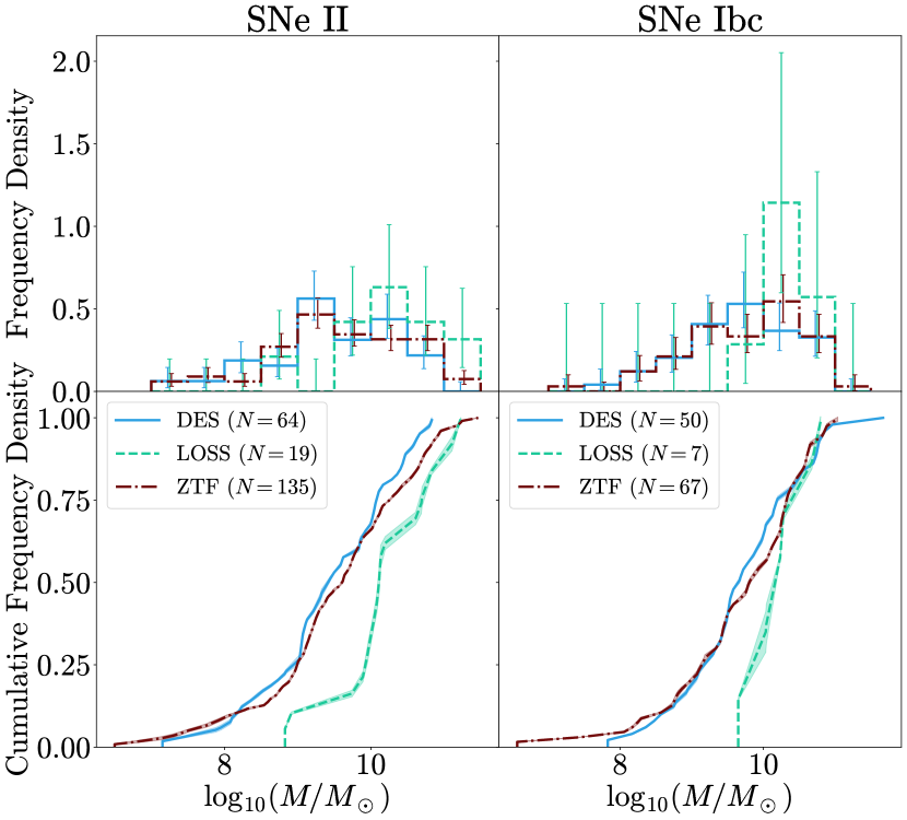
Figure 3: Host galaxy stellar mass distributions and cumulative distributions for SNe II and SNe Ibc for the DES, LOSS and ZTF samples. Histogram uncertainties here (and throughout the paper) are estimated from the Poisson distribution, while CDF uncertainties are estimated from the Monte Carlo approach described in Section 3.2.

4.2 Host rest-frame colours

Fig. 4 shows the distribution of rest-frame $U-R$ colours for the host galaxies in our three samples. For SNe II, we see differences between the three samples: the high-redshift DES sample has the bluest host galaxies, followed by the lower-redshift ZTF sample and then the local LOSS sample. Two-sample KS and AD tests show that the differences between the samples have significances in excess of 3$\sigma$ respectively. For the redshift range considered here, $griz$ does not cover rest-frame $U$-band meaning some extrapolation is involved in calculating $U-R$ for DES hosts. However, we see similar results when using rest-frame $B-V$ which is covered by $griz$. For SNe Ibc, the distributions visually suggest a similar finding however the offset between DES and ZTF is reduced and significance levels are below 2$\sigma$ for $U-R$ and below 2.3$\sigma$ for $B-V$.

Figure 4: As Fig. 3, but for the host galaxy rest-frame $U-R$ colour in place of stellar mass.

Fig. 5 shows host galaxy stellar mass plotted against host galaxy rest-frame $U-R$ colour for each of the three samples, with the thicker symbols showing the mean and standard error for each property across galaxies in bins of $8.25<\log(M/M_{\odot})<9.25$, $9.25<\log(M/M_{\odot})<10.25$ and $10.25<\log(M/M_{\odot})<11.25$ for each sample. Across DES, ZTF and LOSS we see strong correlations between host stellar mass and host $U-R$ colour. This plot also shows that the difference we see in rest-frame $U-R$ colour between DES and ZTF is observed across the range of host galaxy masses in the DES sample, i.e., at fixed stellar mass the DES host galaxy sample is bluer, with this difference more pronounced for SNe II.

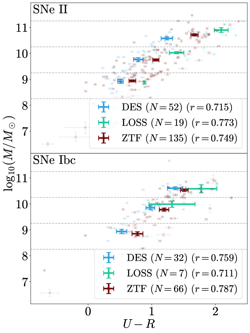
Figure 5: Host galaxy stellar mass plotted against host galaxy rest-frame $U-R$ colour for each sample along with correlation coefficients for each. Thick data points represent the mean and standard error for stellar mass and colour for each sample in stellar mass bins of $8.25<\log(M/M_{\odot})<9.25$, $9.25<\log(M/M_{\odot})<10.25$ and $10.25<\log(M/M_{\odot})<11.25$. The horizontal dashed lines mark these bin boundaries.

Table 4: The results of two-sample KS and AD tests between the distributions of host galaxy stellar mass, rest-frame $U-R$ and $B-V$ colour. Also shown are metallicity values derived from stellar mass in Section 5.2.4 and $U-R$ (SFRcorr) and $U-R$ (Zcorr), the rest-frame $U-R$ colour corrected for SFR and metallicity evolution with redshift introduced in Section 5.3.3.

Property	Survey 1	Survey 2	KS test significance		AD test significance
			SNe II	SNe Ibc	SNe II	SNe Ibc
Stellar mass	DES	LOSS	3.2$\sigma$	2.0$\sigma$	3.4$\sigma$	1.9$\sigma$
	DES	ZTF	0.4$\sigma$	0.5$\sigma$	0.8$\sigma$	0.3$\sigma$
	LOSS	ZTF	3.4$\sigma$	1.5$\sigma$	2.9$\sigma$	1.4$\sigma$
$U-R$	DES	LOSS	4.7$\sigma$	1.9$\sigma$	4.8$\sigma$	2.6$\sigma$
	DES	ZTF	3.4$\sigma$	1.6$\sigma$	3.8$\sigma$	1.8$\sigma$
	LOSS	ZTF	2.7$\sigma$	1.4$\sigma$	3.7$\sigma$	2.0$\sigma$
$B-V$	DES	LOSS	4.3$\sigma$	2.1$\sigma$	4.8$\sigma$	2.7$\sigma$
	DES	ZTF	3.6$\sigma$	1.9$\sigma$	3.9$\sigma$	2.3$\sigma$
	LOSS	ZTF	2.6$\sigma$	1.5$\sigma$	3.7$\sigma$	2.2$\sigma$
Metallicity	DES	LOSS	4.0$\sigma$	2.4$\sigma$	4.0$\sigma$	2.2$\sigma$
	DES	ZTF	1.4$\sigma$	0.9$\sigma$	1.8$\sigma$	0.8$\sigma$
	LOSS	ZTF	3.5$\sigma$	1.5$\sigma$	3.0$\sigma$	1.5$\sigma$
$U-R$ (SFRcorr)	DES	LOSS	4.3$\sigma$	1.4$\sigma$	4.7$\sigma$	2.0$\sigma$
	DES	ZTF	3.0$\sigma$	0.9$\sigma$	3.4$\sigma$	1.3$\sigma$
	LOSS	ZTF	2.8$\sigma$	1.4$\sigma$	3.6$\sigma$	2.0$\sigma$
$U-R$ (Zcorr)	DES	LOSS	3.8$\sigma$	1.6$\sigma$	4.5$\sigma$	2.4$\sigma$
	DES	ZTF	2.4$\sigma$	0.9$\sigma$	2.8$\sigma$	1.0$\sigma$
	LOSS	ZTF	2.7$\sigma$	1.4$\sigma$	3.6$\sigma$	2.1$\sigma$

4.3 Relations between SN and Host Properties

We next consider the relations between the properties of the SNe and the properties of the host galaxies for the three samples.

4.3.1 SNe II/Ibc host properties comparison

Fig. 6 and Fig. 7 show the distributions of host stellar mass and $U-R$ colour comparing the host galaxies of SNe II and Ibc, and Table 5 shows the results of two-sample KS tests between these distributions. For host stellar mass, we do not see any significant differences between the hosts of SNe II and SNe Ibc. We also see no significant difference in host $U-R$ colour for LOSS and ZTF, the latter consistent with the findings of Perley et al. (2020). For the DES sample, the hosts of SNe Ibc appear slightly redder with a significances of 2.0$\sigma$ from the KS and AD tests. Taking $U-R$ as a proxy for star formation rate, this could indicate that SNe Ibc are exploding in galaxies with less star formation than SNe II. SNe Ibc have been shown to trace galaxy star formation more closely than SNe II (e.g., Anderson & James, 2009; Galbany et al., 2018) which would makes this result surprising, albeit with the caveats that these differences refer to local properties rather than the global host properties we present here and that the significance level is not high.

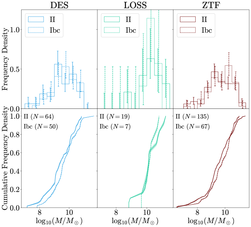
Figure 6: Host galaxy stellar mass distributions and cumulative distributions for each of the DES, LOSS and ZTF samples showing the properties of the hosts of SNe II and SNe Ibc for each sample.

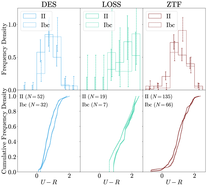
Figure 7: As Fig. 6, but for host galaxy rest-frame $U-R$ colour instead of stellar mass.

Table 5: The results of two-sample KS tests between the SNe II and SNe Ibc host properties in each survey.

Property	Survey	KS test significance	AD test significance
Stellar mass	DES	1.1$\sigma$	1.4$\sigma$
	LOSS	0.1$\sigma$	0.2$\sigma$
	ZTF	1.2$\sigma$	1.3$\sigma$
$U-R$	DES	2.0$\sigma$	2.0$\sigma$
	LOSS	0.1$\sigma$	0.2$\sigma$
	ZTF	1.8$\sigma$	1.5$\sigma$

4.3.2 SN/host correlations

We also consider relations between the properties of the host galaxy and the properties of the SN, looking at correlations between peak SN luminosity and host stellar mass and rest-frame colour. Table 6 shows the Pearson correlation coefficients ($r$) between these properties for each of the DES, LOSS and ZTF samples.

For both SN II and SN Ibc samples, we see no obvious or significant trends between the SN luminosities and the properties of the galaxies that host them – the correlations seen for SNe Ibc in LOSS are not statistically significant and correspond to only 7 galaxies. Gutiérrez et al. (2018) also finds no relation between stellar mass and peak SN luminosity for SNe II, and Wiseman et al. (2020b) finds a lack of strong evidence for a relation between peak transient luminosity and host mass and sSFR for RETs.

Table 6: Correlation coefficients between peak SN $R$-band absolute magnitude and host galaxy stellar mass and rest-frame $U-R$ colour for SNe II and Ibc in DES, LOSS and ZTF.

Property	Survey	SN Type	Correlation with SN peak
			$R$-band absolute magnitude (r)
Stellar mass	DES	II	0.09
		Ibc	0.03
	LOSS	II	-0.28
		Ibc	0.57
	ZTF	II	-0.12
		Ibc	0.14
$U-R$	DES	II	-0.06
		Ibc	0.07
	LOSS	II	-0.12
		Ibc	0.55
	ZTF	II	0.07
		Ibc	0.21

5 Discussion

In this section we explore our results, considering and assessing a number of potential causes for some of the noteworthy trends that we observe.

5.1 Impact of photometric misclassification

We begin by discussing the potential impact of misclassification of the sample of photometric CCSNe with host spec-z in DES. SNe Ia have been removed using SuperNNova model presented in Vincenzi et al. (2021a), which has a high degree of accuracy upward of 98 per cent. As discussed in Section 2.1.2, the pSNid model used to split this sample into SNe II and Ibc has an accuracy of 86 per cent on the sample of DES CCSNe with spectroscopic classifications, with similar performance on each of the two classes. While this method works well, it does leave open the possibility that a small proportion of SNe in this sample are assigned to the wrong class.

To investigate what effect this may have on our analysis, we repeat the Monte Carlo process for CDF uncertainty outlined in Section 3.2 but this time in each iteration we flip 14 per cent of the classes, corresponding to the expected error rate, for the photometrically classified DES CCSNe (SNe II are changed to SNe Ibc and vice versa) to see what effect this has on the final CDF. Fig. 8 shows the luminosity functions and host galaxy $U-R$ distributions for the three samples, with the randomised class flipping applied to DES photometrically classified SNe. Overall, these distributions appear very similar to those in Fig. 2 and 4 and the incorporation of the class flipping has little effect. We also try restricting the sample to only spectroscopically confirmed supernovae from DES and see the same trends for SNe II, although there are too few spectroscopically confirmed SNe Ibc to make this comparison.

Considering the overall samples after quality cuts, but before redshift and magnitude cuts, the final ZTF sample consists of 174 SNe II and 89 SNe Ibc, a ratio of $\sim$2:1. In contrast, the photometrically confirmed sample with hosts spectroscopic redshifts from DES consists of 56 SNe II and 42 SNe Ibc at a ratio of $\sim$1.33:1. At first glance, this suggests that pSNid is classifying too many objects as SNe Ibc. However, it is important also to consider the spectroscopically confirmed sample from DES - as this sample is based on targeted follow-up, it would not be expected to follow the same ratio of classes as an untargeted sample such as ZTF. Combining both these DES samples, there are 89 SNe II and 55 SNe Ibc, a ratio of $\sim$1.75:1 which is much closer to ZTF. After redshift and magnitude cuts, this ratio shifts further from 2:1, but the relatively small sample sizes compared with ZTF mean this is not surprising. Overall, we consider the results presented in this analysis robust to the potential misclassification of SNe II and Ibc.

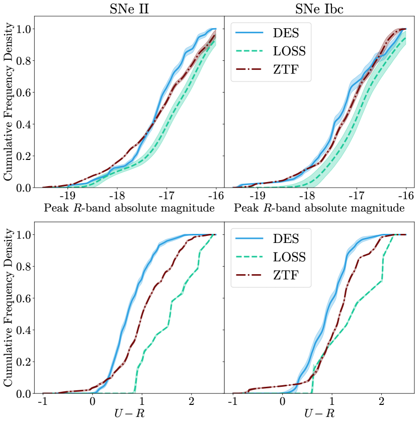
Figure 8: CDFs for the luminosity functions and rest-frame host galaxy $U-R$ colours for each of the DES, LOSS and ZTF samples, incorporating a 14 per cent misclassification rate for photometrically classified SNe in DES as outlined in Section 5.1.

5.2 Difference in the luminosity function

As part of our analysis, we have carried out two-sample KS tests between the luminosity functions of DES, LOSS and ZTF. For SNe II, DES is brighter than LOSS at a significance level of 3.0$\sigma$ and appears brighter than ZTF although only at a significance of 1.8$\sigma$. For SNe Ibc, DES also appears brighter than both LOSS and ZTF although at a significances of only 1.9$\sigma$ and 1.1$\sigma$. Although the significance levels are not high, these differences raise the possibility of underlying differences in the luminosity functions of these samples. If there is a difference, one natural explanation would be redshift evolution in the underlying stellar populations and progenitor stars. However, we first consider other, simpler explanations.

5.2.1 Incompleteness

The most straight forward explanation for any difference between DES and LOSS is a lack of completeness in the DES sample due to lower sensitivity to fainter SNe. Fig. 1 shows the peak absolute magnitudes of all objects in our samples plotted against redshift, prior to making any selection in absolute magnitude. Fig. 2 shows the main differences between DES and LOSS for SNe II are in the [$-16$, $-16.5$] luminosity bin and for SNe Ibc are in the [$-16$, $-16.7$]. DES is not complete in this range and the distribution is affected by the $V_{\text{max}}$ correction, whereas the LOSS sample is not affected by this correction. The $V_{\text{max}}$ correction for DES gives a maximum weighting of  2.9 but for ZTF this is much higher due to the lack of completeness in the sample, up to a maximum of 14.5 although this is typically around 2-3. We can mitigate for this with lower redshift cuts for DES and ZTF to obtain more complete samples – doing so reduces the significances from the KS test due to the smaller sample size but overall the trends that we see appear unchanged. This suggests that incompleteness is not the cause of potential differences between the samples.

5.2.2 Host Properties

An alternative possibility is that any difference in luminosity function could be explained by a difference in host properties between the samples. For example, the host galaxies of the LOSS sample are significantly more massive and redder than that of DES, likely because of the galaxy-targeted nature of LOSS (Section 4). However, as there are no significant correlations between either host colour or mass and peak SN luminosity (Section 4.3) this is unlikely to cause any differences in the luminosity function.

5.2.3 Host Extinction

The difference in luminosity function could also result from differing levels of host galaxy extinction between the two samples. This could be due to both global and local host properties; for example, on average we might expect a higher level of host extinction in more massive, redder, dustier host galaxies and SNe closer to the central dusty regions of the host.

The DES hosts are, on average, bluer than those of LOSS and ZTF, which could indicate higher levels of host extinction in LOSS and ZTF that might explain any differences we see. To explore this possibility, we compare the luminosity functions of LOSS and ZTF with only SNe in DES that are in redder host galaxies. When we make cuts at either $U-R>0.5$, $U-R>0.75$ or $U-R>1.0$, while the KS test significances are reduced by the smaller sample size we find that the same overall trends are observed as for the full sample. This would indicate that differing levels of host extinction do not cause any differences we see, though without measurements of the host extinction we cannot rule this out as a possibility – local environment properties are likely to play a significant part in the level of extinction. We also consider the possibility of differing SN radial distributions across the three samples leading to differing levels of extinction, but do not find any significant differences in the physical separation between SN and host.

5.2.4 Metallicity

Differences in metallicity may also explain potential differences in the luminosity functions; for example, DES SNe may occur in lower metallicity environments than LOSS or ZTF. As previously mentioned, host metallicity affects the supernova population as the most luminous classes of supernovae preferentially occur in low-mass, low-metallicity environments. Metallicity varies with stellar mass, star formation rate, redshift (e.g. Zahid et al. 2013; Yates et al. 2012; Curti et al. 2020) and also radially within a galaxy (Parikh et al., 2021). There are a number of reasons why the DES hosts could be expected to be lower metallicity than either the LOSS or ZTF hosts: the DES hosts are lower stellar mass than those of LOSS, they are bluer and hence more star forming than hosts in ZTF or LOSS (although the effect of increased SFR on metallicity will vary depending on galaxy mass) and they are at higher redshift. Metallicity differences are a possible cause of any differences in luminosity function.

While we do not have metallicity values calculated from host galaxy spectroscopy, we can get an indication of global host galaxy metallicity using the relation between stellar mass and metallicity given in equation 4 of Zahid et al. (2013). We calculate global galaxy metallicity using following approach:

• We fit a straight line to the relation between the redshifts and mass-metallicity relation parameters quoted in Table 1 of Zahid et al. (2013). We use only the samples from SDSS, the Smithsonian Hectospec Lensing Survey (SHELS; Geller et al., 2014) and the DEEP2 survey (Newman et al., 2013) quoted here as the higher redshift samples have very uncertain values for these parameters.

• For a galaxy at a given redshift, we use these linear fits to estimate the mass-metallicity relation parameters at that redshift and then use the relation at that redshift to convert our measured stellar mass from SED fits to a metallicity.

The results of two-sample KS and AD tests between the global host metallicities of each of our samples are shown in Table 4 - as for stellar mass, DES and ZTF are consistent while both show differences to LOSS. Of course, in reality there will be a large degree of scatter around the mass-metallicity relation. However, this indicates differing host metallicity could explain differences between DES and ZTF but not between DES and LOSS.

We can also probe metallicity looking at the decline rates during the plateau phase after maximum light of SNe II. Theoretical models suggest that the metallicity of the progenitor star may affect the decline rate during the ‘plateau’ phase of the SN light curve (Dessart et al., 2013b), however, observations do not show this dependence (Anderson et al., 2016). The absence of correlations could be related to the lack of SNe II in low-luminosity hosts. Nevertheless, some relations can be established when SNe II in faint hosts are included. Gutiérrez et al. (2018) find that slow-decliner SNe II (i.e. SNe with lower s2 values) occur preferentially in low-luminosity (and therefore low-metallicity) hosts. For SNe II in DES and ZTF, we calculate the decline rate of this phase of the light curve (corresponding to s2 in Anderson et al., 2014) and find that the decline rates calculated are consistent across the two samples. This suggests that there is not a significant metallicity difference between the two samples, indicating that this is unlikely to explain any differences between DES and ZTF.

5.2.5 Summary

The notion of a luminosity function which evolves with redshift is an interesting one - the differences we see in the luminosity functions of SNe II in DES and LOSS and SNe Ibc in DES, LOSS and ZTF raise this as a possibility, with the caveat that the significances are not especially high. Any differences could be explained by a lack of completeness in the DES sample, however this will have been significantly mitigated for by the $V_{max}$ correction and making a lower redshift cut does not change the trends we see. Greater dust extinction from redder host galaxies is another possible explanation given that LOSS and ZTF hosts are bluer than DES, but selecting only DES SNe in redder hosts or ZTF and LOSS SNe in bluer hosts does not change the trends we see which suggests that this is not the case - despite this, without measurements of the host extinction we cannot rule this out as a possibility. Differing metallicity also does not seem to explain the differences as we see consistent global host galaxy metallicities between DES and ZTF using the mass-metallicity relation of Zahid et al. (2013) and consistent decline rates after peak for SNe II.

5.3 Host galaxy colour discrepancy

Section 4.2 uncovered a puzzling trend: SNe II in DES on average occur in bluer galaxies than those in ZTF and LOSS. A difference in host galaxy properties between DES/ZTF and LOSS can be explained, at least in part, by the differences in targeting between the surveys. However, the difference in host rest-frame colour between DES and ZTF is not so easily understood. In this section we explore possible explanations for this difference.

5.3.1 DES spectroscopic selection bias

The DES sample in Fig. 4 contains only CCSNe with a spectroscopic host redshift, obtained from a variety of sources (Vincenzi et al., 2021b). Typically, galaxy redshifts are measured through the presence of narrow emission lines in their spectra, which will generally be stronger in bluer, star-forming galaxies. This may lead to a bias towards bluer galaxies in the DES sample, although Vincenzi et al. (2021b) finds that the difference in spectroscopic selection efficiency in DES between red and blue galaxies is small. By contrast, ZTF has an automated SN spectroscopic follow-up programme which provides redshift information for 93 per cent of observed transients with $m<18.5$ mag and 100 per cent with $m<17$ mag. As a result, any possible bias affecting DES would not affect ZTF.

We compare the DES samples with host spec-zs (both the spectroscopically confirmed and photometric with spec-z samples) and ZTF samples to the DES CCSN sample with only photo-zs. (Fig. 9). However, rather than explaining the difference in host colour, this photometric sample appears bluer than the DES spec-z sample. Considering the host stellar mass distribution for this sample, this is not unexpected: the DES hosts without spectroscopic redshifts are low stellar mass galaxies which are typically bluer and more strongly star-forming than higher mass galaxies. In summary, the difference in host rest-frame colour cannot be easily explained by a simple spectroscopic selection bias in DES.

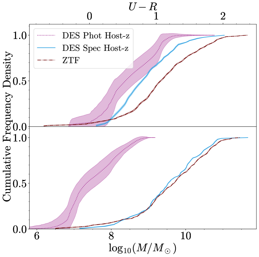
Figure 9: Host galaxy rest-frame $U-R$ (top) and stellar mass (bottom) cumulative distributions for all CCSNe in the the DES sample of objects without spectroscopic host redshifts, compared with the DES sample with spectroscopic host redshifts as well as the ZTF sample.

5.3.2 ZTF spectroscopic selection effects

An alternative explanation is some selection bias in ZTF which favours SNe in redder hosts. The ZTF BTS sample has a very high level of spectroscopic completeness; however, spectroscopy is not captured exclusively by the ZTF spectroscopic instrument SEDMachine (SEDM) – in cases where the SEDM spectra are unreliable other instruments may be used, and in cases where an object is first classified by another survey ZTF do not take an additional spectrum. To understand whether this may introduce selection effects, we examine the sub-sample of ZTF SNe only with a classification reported by SEDM. However, we find no significant difference in this population: a two-sample KS test between the $U-R$ host colour distributions of DES and only ZTF SNe classified by SEDM has a significance of 3.2$\sigma$ and 3.4$\sigma$ from KS and AD tests, almost unchanged from the full ZTF sample.

5.3.3 Redshift evolution of the host galaxies

Another possible explanation is redshift evolution, with a period of $\sim$1–2 Gyr between most of the ZTF and DES SNe exploding. ZTF hosts are therefore on average older and less strongly star-forming. The host galaxy SFRs can be corrected for redshift evolution following the method of section 4.2 of Taggart & Perley (2021), based on the star-forming sequences of thousands of galaxies outlined in Salim et al. (2007) and Noeske et al. (2007), correcting the SFR values to $z=0$. However, we do not measure SFR directly, and instead measure $U-R$ colour. We adapt the Taggart & Perley (2021) method to $U-R$ using the following steps:

• We calculate the SFR correction for each galaxy; this correction will be the same for sSFR as well.

• We fit a linear relationship between $U-R$ colour and sSFR for all host galaxies in our sample.

• We use the gradient of this line to convert the sSFR correction into a $U-R$ correction.

We can then compare the distributions of these corrected colours with those of the ZTF hosts.

Fig. 10 shows the distributions of rest-frame $U-R$ colour corrected for the evolution of SFR, hereafter $U-R$ (SFRcorr). The correction factor between typical DES and ZTF redshifts is $\simeq 0.03$–$0.04$ mag and thus the effect is small: the significance of the difference between DES and ZTF from the two-sample KS test is reduced by only 0.4$\sigma$. Based on this, the difference in host colour seems unlikely to be caused by redshift evolution of the underlying galaxy populations.

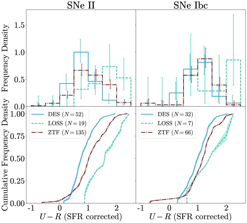
Figure 10: Host galaxy rest-frame $U-R$ colour distributions and cumulative distributions, corrected for the effects of SFR evolution with redshift, for both SNe II and SNe Ibc for DES, LOSS and ZTF samples.

However, another redshift evolution we should consider is the evolution of the mass-metallicity relation with redshift. The metallicity of the host galaxies will have an effect on the emission lines produced, which will in turn affect galaxy colour. To investigate this, we use the following process to correct $U-R$ colour for the effects of metallicity evolution:

• Fit a relation between our metallicity values inferred from Zahid et al. (2013) discussed in Section 5.2.4 and our rest-frame host galaxy $U-R$ colours. Unlike the SFR correction, this relationship is not linear. Instead, we fit an exponential relation with a linear term of the form $y=mx+c+e^{A(x-x_{0})}$ where $m$, $c$, $A$ and $x_{0}$ are the fitting parameters.

• Compare the metallicity difference for each galaxy of a given mass between its actual redshift and $z=0$.

• Use the fitted relation between metallicity and $U-R$ to estimate how much this change in metallicity would affect the rest-frame $U-R$ colour.

• Modify our calculated $U-R$ colours by this correction factor to calculate the rest-frame $U-R$ colour corrected for metallicity evolution, hereafter $U-R$ (Zcorr).

This correction involves the use of two relations which show a large degree of scatter, the mass-metallicity relation from Zahid et al. (2013) and our relation between $U-R$ colour and metallicity. However, this does give an indication of the extent that evolving metallicity will have on $U-R$ colour.

Fig. 11 shows the distributions of $U-R$ (Zcorr). This correction factor is larger than the previous correction for SFR evolution. For SNe II, this correction reduces the gap between DES and ZTF and the significance of this offset is reduced to 2.4$\sigma$ and 2.8$\sigma$ for both KS and AD tests, however the offset in $U-R$ between DES and ZTF across different galaxy masses as in Fig. 5 is still seen. Overall, metallicity evolution with redshift may explain some but not all of the offset in rest-frame $U-R$ colour between host galaxies in DES and ZTF.

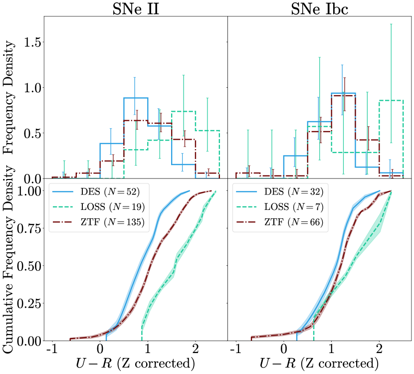
Figure 11: Host galaxy rest-frame $U-R$ colour distributions and cumulative distributions, corrected for the effects of metallicity evolution with redshift, for both SNe II and SNe Ibc for DES, LOSS and ZTF samples.

5.3.4 Systematic differences in photometry used

An additional possibility is that the difference sources of host galaxy photometry between DES and ZTF is causing some systematic offset between the two samples. It may be that the inclusion of $u$-band data in the SED fits for the ZTF hosts is causing a systematic difference compared with the $griz$-only SED fits for the DES hosts (Section 2.4). We remove the $u$-band data from the ZTF host photometry and repeat the SED fits using only $griz$, but find that the ZTF rest-frame colours from $griz$ fits are consistent with those from $ugriz$ fits and thus that the difference between DES and ZTF host colours remains.

Alternatively, there may be differences between DES and SDSS photometry which cause an offset when considering the same bands. To investigate this possibility, we match DES supernovae to the SDSS host catalogue using a 5″search radius, finding 47 objects with SDSS host galaxies. We then repeat the SED fits using SDSS photometry instead of DES. We find that rest-frame $U-R$ colours from SDSS photometry are consistent with those from DES with no systematic offset between the two. Overall, the difference in host colour does not seem to be caused by systematic differences in the data used to calculate host properties.

5.3.5 Summary

In summary, the difference in host galaxy rest-frame colour between the ZTF and DES samples is not obviously caused by selection biases in the two samples or systematic differences in the SED fitting for DES and ZTF, and metallicity evolution with redshift can only partially explain this offset. We further note that the difference in host colour is much more pronounced in the SN II host sample: if there were some overall systematic bias, we would expect to see the same effect in the SN Ibc sample as well. It remains unclear what may be driving the difference in host colour, and more data is required to study this in further detail.

6 Conclusions

DES provides a large sample of high-redshift spectroscopically and photometrically-confirmed CCSNe. We derive rest-frame luminosity functions for the DES sample using SED models to K-correct to the rest-frame and GP-interpolations to estimate the peak luminosity. Using the deep $griz$ DES host photometry from Wiseman et al. (2020a), we calculate the host properties of the DES sample using SED fits. To examine any selection biases in the sample and investigate the possible effect of redshift evolution on the luminosity function and host properties, we also compare SN and host properties to a low redshift CCSN sample from LOSS and an intermediate redshift sample from ZTF. From this comparison, our main conclusions are as follows:

1. We present luminosity functions of SNe II and SNe Ibc for DES, LOSS and ZTF, incorporating a $V_{max}$ correction to mitigate for the effects of Malmquist bias. Where we see a peak in the luminosity function, we fit Gaussian and Lorentzian distributions and present the parameter values to allow these to be used to simulate CCSN samples.

2. We explore differences between the DES luminosity functions. The DES luminosity functions appears brighter than those of LOSS and ZTF, with differences of significance level 3.0$\sigma$ and 1.8$\sigma$ to each survey for SNe II and 1.9$\sigma$ and 1.1$\sigma$ for SNe Ibc. This could result from higher levels of host galaxy extinction in LOSS and ZTF, however selecting a subset of DES SNe which explode in redder host galaxies does not change the trends we see which suggests this is not the case. This raises the possibility of a luminosity function which evolves with redshift, although at the significance levels we calculate we cannot be sure that any differences are real. Were these effects real, we also cannot rule out causes such as differing host extinction without measurements of this.

3. There are differences in the host galaxy properties of the LOSS CCSNe compared to the DES and ZTF CCSNe, but these are expected given that LOSS is a galaxy-targeted survey while DES and ZTF are untargeted.

4. There are also differences in the host galaxy properties of DES CCSNe compared with those in ZTF. The host galaxy stellar masses of both samples are consistent across both SNe II and SNe Ibc. However for SNe II, DES host galaxies are significantly bluer than the ZTF hosts with a significance levels of 3.4$\sigma$ and 3.8$\sigma$ from two-sample KS and AD tests respectively.

5. We explore correcting the host galaxy colours to account for redshift evolution, and study the possibility that this difference is caused by selection biases in the DES or ZTF samples or systematic differences in the data used, but find that none of the are able to adequately explain the differences.

6. The host masses and rest-frame $U-R$ colours of SNe II compared to SNe Ibc are generally consistent in both the LOSS and ZTF samples. In the DES sample, hosts of SNe II appear bluer than those of SNe Ibc but only at a significance level of 2.0$\sigma$.

7. Overall, we observe little environmental dependence on SN peak magnitude across the three samples.

Data Availability Statement

The data underlying this article, as well as the observed DES-SN photometry, are available in the article and in its online supplementary material. The ZTF photometry used can be accessed through the Lasair broker (https://lasair.roe.ac.uk/).

Affiliations

¹ School of Physics and Astronomy, University of Southampton, Southampton, SO17 1BJ, UK
² Finnish Centre for Astronomy with ESO (FINCA), FI-20014 University of Turku, Finland
³ Tuorla Observatory, Department of Physics and Astronomy, FI-20014 University of Turku, Finland
⁴ Institute of Cosmology and Gravitation, University of Portsmouth, Portsmouth, PO1 3FX, UK
⁵ Institut d’Estudis Espacials de Catalunya (IEEC), 08034 Barcelona, Spain
⁶ Institute of Space Sciences (ICE, CSIC), Campus UAB, Carrer de Can Magrans, s/n, 08193 Barcelona, Spain
⁷ Centre for Astrophysics & Supercomputing, Swinburne University of Technology, Victoria 3122, Australia
⁸ Center for Astrophysics $|$ Harvard & Smithsonian, 60 Garden Street, Cambridge, MA 02138, USA
⁹ School of Mathematics and Physics, University of Queensland, Brisbane, QLD 4072, Australia
¹⁰ Centre for Gravitational Astrophysics, College of Science, The Australian National University, ACT 2601, Australia
¹¹ The Research School of Astronomy and Astrophysics, Australian National University, ACT 2601, Australia
¹² Department of Physics, Duke University Durham, NC 27708, USA
¹³ Cerro Tololo Inter-American Observatory, NSF’s National Optical-Infrared Astronomy Research Laboratory, Casilla 603, La Serena, Chile
¹⁴ Laboratório Interinstitucional de e-Astronomia - LIneA, Rua Gal. José Cristino 77, Rio de Janeiro, RJ - 20921-400, Brazil
¹⁵ Fermi National Accelerator Laboratory, P. O. Box 500, Batavia, IL 60510, USA
¹⁶ Department of Physics, University of Michigan, Ann Arbor, MI 48109, USA
¹⁷ Centro de Investigaciones Energéticas, Medioambientales y Tecnológicas (CIEMAT), Madrid, Spain
¹⁸ CNRS, UMR 7095, Institut d’Astrophysique de Paris, F-75014, Paris, France
¹⁹ Sorbonne Universités, UPMC Univ Paris 06, UMR 7095, Institut d’Astrophysique de Paris, F-75014, Paris, France
²⁰ University Observatory, Faculty of Physics, Ludwig-Maximilians-Universität, Scheinerstr. 1, 81679 Munich, Germany
²¹ Department of Physics & Astronomy, University College London, Gower Street, London, WC1E 6BT, UK
²² Instituto de Astrofisica de Canarias, E-38205 La Laguna, Tenerife, Spain
²³ Universidad de La Laguna, Dpto. Astrofísica, E-38206 La Laguna, Tenerife, Spain
²⁴ INAF-Osservatorio Astronomico di Trieste, via G. B. Tiepolo 11, I-34143 Trieste, Italy
²⁵ Center for Astrophysical Surveys, National Center for Supercomputing Applications, 1205 West Clark St., Urbana, IL 61801, USA
²⁶ Department of Astronomy, University of Illinois at Urbana-Champaign, 1002 W. Green Street, Urbana, IL 61801, USA
²⁷ Institut de Física d’Altes Energies (IFAE), The Barcelona Institute of Science and Technology, Campus UAB, 08193 Bellaterra (Barcelona) Spain
²⁸ Astronomy Unit, Department of Physics, University of Trieste, via Tiepolo 11, I-34131 Trieste, Italy
²⁹ Institute for Fundamental Physics of the Universe, Via Beirut 2, 34014 Trieste, Italy
³⁰ Hamburger Sternwarte, Universität Hamburg, Gojenbergsweg 112, 21029 Hamburg, Germany
³¹ Department of Physics, IIT Hyderabad, Kandi, Telangana 502285, India
³² Jet Propulsion Laboratory, California Institute of Technology, 4800 Oak Grove Dr., Pasadena, CA 91109, USA
³³ Institute of Theoretical Astrophysics, University of Oslo. P.O. Box 1029 Blindern, NO-0315 Oslo, Norway
³⁴ Kavli Institute for Cosmological Physics, University of Chicago, Chicago, IL 60637, USA
³⁵ Instituto de Fisica Teorica UAM/CSIC, Universidad Autonoma de Madrid, 28049 Madrid, Spain
³⁶ Department of Physics and Astronomy, University of Pennsylvania, Philadelphia, PA 19104, USA
³⁷ Observatório Nacional, Rua Gal. José Cristino 77, Rio de Janeiro, RJ - 20921-400, Brazil
³⁸ Santa Cruz Institute for Particle Physics, Santa Cruz, CA 95064, USA
³⁹ Center for Cosmology and Astro-Particle Physics, The Ohio State University, Columbus, OH 43210, USA
⁴⁰ Department of Physics, The Ohio State University, Columbus, OH 43210, USA
⁴¹ Australian Astronomical Optics, Macquarie University, North Ryde, NSW 2113, Australia
⁴² Lowell Observatory, 1400 Mars Hill Rd, Flagstaff, AZ 86001, USA
⁴³ Sydney Institute for Astronomy, School of Physics, A28, The University of Sydney, NSW 2006, Australia
⁴⁴ Institució Catalana de Recerca i Estudis Avançats, E-08010 Barcelona, Spain
⁴⁵ Physics Department, 2320 Chamberlin Hall, University of Wisconsin-Madison, 1150 University Avenue Madison, WI 53706-1390
⁴⁶ Department of Astronomy, University of California, Berkeley, 501 Campbell Hall, Berkeley, CA 94720, USA
⁴⁷ Institute of Astronomy, University of Cambridge, Madingley Road, Cambridge CB3 0HA, UK
⁴⁸ Department of Astrophysical Sciences, Princeton University, Peyton Hall, Princeton, NJ 08544, USA
⁴⁹ Centro de Investigaciones Energéticas, Medioambientales y Tecnológicas (CIEMAT), Av. Complutense, 22, E- 28040 Madrid, Spain
⁵⁰ Department of Physics and Astronomy, Pevensey Building, University of Sussex, Brighton, BN1 9QH, UK
⁵¹ Kavli Institute for Particle Astrophysics & Cosmology, P. O. Box 2450, Stanford University, Stanford, CA 94305, USA
⁵² SLAC National Accelerator Laboratory, Menlo Park, CA 94025, USA
⁵³ Computer Science and Mathematics Division, Oak Ridge National Laboratory, Oak Ridge, TN 37831
⁵⁴ Excellence Cluster Origins, Boltzmannstr. 2, 85748 Garching, Germany
⁵⁵ Max Planck Institute for Extraterrestrial Physics, Giessenbachstrasse, 85748 Garching, Germany
⁵⁶ Universitäts-Sternwarte, Fakultät für Physik, Ludwig-Maximilians Universität München, Scheinerstr. 1, 81679 München, Germany

Appendix A Estimating host properties using photometric redshifts

For the DES-SN sample of CCSNe with only photometric host redshifts, we estimate host galaxy properties using the following Monte Carlo (MC) process:

• For each object, we have 0.5th, 2.5th, 16th, 84th, 97.5th and 99.5th percentiles of the photometric redshift distribution. Studying the cumulative distributions of these values shows the distribution to be approximately Gaussian - as such, we model the redshift distribution of each host as a Gaussian, estimating the mean and standard deviation of this Gaussian by fitting a generalised error function to our cumulative distribution.

• We use the $griz$ photometry of each host from the DES deep coadded host images to estimate the properties of the host, following the same SED fitting process as for objects with spectroscopic redshift information. We do this for every redshift between the 0.5 and 99.5 percentiles in the redshift distribution of each host, in intervals of 0.001. This gives the properties the host galaxy would have were it located at each redshift in this distribution.

• For each host galaxy, we draw a random redshift from a Gaussian distribution using our estimates of mean and standard deviation. We then select the properties of each host galaxy at these redshifts and use these to produce a CDF for each host property for this randomised sample. (If a randomised redshift lies outside the redshift range of our spectroscopic sample, it is excluded from the sample.)

• We repeat this 10,000 times in an Monte Carlo process, examining the spread of the CDFs over all iterations to obtain a final CDF with an associated error. This allows us to include the large uncertainties in host redshift into a comparison of the host galaxy properties for different samples.

We find that only including SNe with a randomised redshift of less than 0.25 in each iteration gives a sample size that varies between 3 and 8, and typically 5 or 6. Photometric redshifts are currently only available for three out of the ten DES fields – extrapolating, we would expect there to be between 10–27 CCSNe for which we have DES photometry but no spectroscopic host redshift, and which would otherwise be included in our luminosity functions. Our luminosity function sample contains 98 DES SNe with spectroscopic host redshifts, thus we have spectroscopic host redshifts for $\sim 75-90$ per cent of the CCSNe which should be included in our sample suggesting that these ‘missing’ SNe should not have a significant effect on the luminosity function.

Appendix B SED-fitting analysis for LOSS host galaxies

Fig. 12 shows comparisons with our host properties from SED fitting for the $B$/$K$-band stellar masses and host stellar masses and SFRs from Leroy et al. (2019) and Karachentseva et al. (2020). These were performed with the full LOSS SN sample, without the selection of events used for the SNe in the luminosity functions – this gives 56 host galaxies with properties derived from SED fits to SDSS photometry, 96 host galaxies with $B$/$K$-band masses and 71 with previously published literature values for stellar mass and SFR.

Our stellar masses from SED-fitting are consistent with the $B$/$K$-band masses. The Pearson correlation coefficient ($r$) for these two sets of masses is 0.75 indicating a strong correlation, with a dispersion of 0.39 dex. Comparing our stellar masses from others in the literature gives $r=0.65$ and a dispersion of 0.65 dex. Overall, our masses seem broadly consistent with those derived from other methods. However, the correlation between our SFR values derived from SED fits and those from literature is only $r=0.30$ with a dispersion of 2.17 dex, demonstrating the uncertainties in estimating SFRs from SED fitting which have a stronger dependence on star-formation history. We do not use SFR in our analysis, and instead use rest-frame $U-R$, which is well-constrained by the observed data.

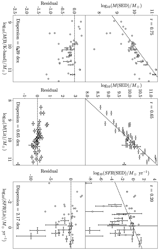
Figure 12: Upper panels: Host galaxy stellar masses and SFRs for LOSS from our SED fits to SDSS $ugriz$ photometry compared with stellar masses derived from the $K$-band mass-to-luminosity ratio presented in L11 and with stellar masses and SFRs presented in Leroy et al. (2019) and Karachentseva et al. (2020). Correlation coefficients are shown, and the dashed line shows a perfect agreement. Lower panels: Residuals from the perfect agreement in the upper panels.

Appendix C ZTF Magnitude Limit for Malmquist Bias Correction

As mentioned in Section 3.1, we consider the 97, 93 and 75 per cent spectroscopic completeness limits of ZTF, $18$, $18.5$ and $19$ mag respectively. The luminosity functions for ZTF with these three limits are shown in figure 13. Above -17 mag, these appear consistent with each other, however these luminosity functions diverge between -16 and -17. A limit of 18 mag omits some SNe in this region and appears to bias the sample in favour of brighter objects. The luminosity functions for a limit of 18.5 and 19 appear consistent with each other - as a result, we settle on a limit of 19 mag to maximise the sample size.

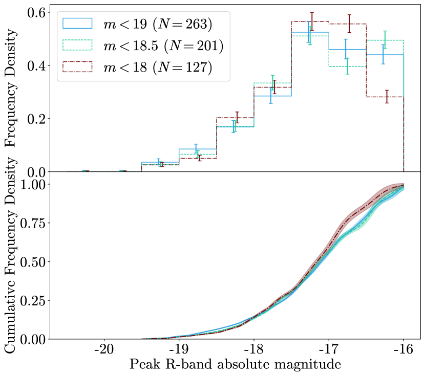
Figure 13: As Fig. 2, but for samples only from ZTF with $V_{max}$ corrections calculated for magnitude limits of 18, 18.5 and 19 mag.

Appendix D Data Tables

Table LABEL:long_table present the peak $R$-band absolute magnitudes and host galaxy properties used for all analysis in this work, for the three different samples. Table 8 presents DECam photometry of the DES sample presented in this paper.

Table 7: Supernova peak $R$-band absolute magnitudes (M${}_{\text{max}}$) and host galaxy properties for the DES, LOSS and ZTF samples presented in this work, along with their associated errors. Please note, objects denoted with ^∗ correspond to two SNe II in ZTF with M${}_{\text{max}}$ less than -16 which have used only for the fits presented in Section 3.3, to help constrain the peak of the luminosity function, and not in the rest of the analysis.

SN	Survey	Class	Source${}^{\text{a}}$	z	M${}_{\text{max}}^{\text{b}}$	err	weight${}^{\text{c}}$	$M^{\text{d}}$	err	$U-R^{\text{e}}$	err	$B-V^{\text{f}}$	err
DES13C2jtx	DES	II	spec	0.223	-18.61	0.03	1.00	10.63	0.02	1.32	0.01	0.72	0.01
DES13X3fca	DES	II	spec	0.096	-16.92	0.02	1.00	10.02	0.01	1.48	0.01	0.69	0.01
DES14C3aol	DES	II	spec	0.076	-16.21	0.02	1.00	10.83	0.02	1.71	0.02	0.89	0.02
DES14X2cy	DES	II	spec	0.232	-18.99	0.01	1.00	9.22	0.02	0.43	0.02	0.38	0.01
DES14X2nzt	DES	II	spec	0.195	-18.31	0.02	1.00	–	–	–	–	–	–
DES15C2eaz	DES	II	spec	0.062	-17.49	0.03	1.00	8.10	0.01	0.78	0.03	0.39	0.02
DES15C2lna	DES	II	spec	0.069	-16.72	0.02	1.39	10.02	0.03	1.07	0.04	0.62	0.02
DES15C2lpp	DES	II	spec	0.181	-17.12	0.04	1.00	10.47	0.01	1.21	0.02	0.65	0.01
DES15C2npz	DES	II	spec	0.123	-17.18	0.02	1.00	9.13	0.01	0.73	0.02	0.46	0.01
DES15E1iuh	DES	II	spec	0.105	-17.14	0.02	1.00	7.44	0.08	0.68	0.14	0.43	0.06
DES15S1by	DES	II	spec	0.129	-17.13	0.03	1.00	9.33	0.04	0.60	0.06	0.40	0.01
DES15S1cj	DES	II	spec	0.167	-18.16	0.02	1.00	10.17	0.01	1.33	0.02	0.71	0.01
DES15S1lrp	DES	II	spec	0.223	-18.44	0.02	1.00	8.36	0.05	0.71	0.10	0.41	0.05
DES15S2eaq	DES	II	spec	0.068	-16.37	0.03	2.09	9.22	0.01	0.69	0.02	0.44	0.01
DES15X2mku	DES	II	spec	0.09	-16.67	0.02	1.47	8.73	0.04	–	–	0.36	0.02
DES15X3mpq	DES	II	spec	0.188	-17.55	0.02	1.00	10.29	0.01	1.00	0.02	0.56	0.01
DES15X3nad	DES	II	spec	0.10	-18.15	0.03	1.00	–	–	–	–	–	–
DES16C1cbg	DES	II	spec	0.111	-16.99	0.02	1.02	9.07	0.01	0.85	0.03	0.51	0.01
DES16C2cbv	DES	II	spec	0.109	-17.37	0.03	1.00	8.08	0.02	0.10	0.02	0.25	0.01
DES16X2bkr	DES	II	spec	0.159	-17.42	0.02	1.00	8.20	0.02	–	–	0.31	0.02
DES16X3cpl	DES	II	spec	0.205	-17.29	0.01	1.00	9.07	0.03	–	–	0.59	0.03
DES17C2pf	DES	II	spec	0.135	-17.22	0.02	1.00	7.15	0.14	0.39	0.23	0.34	0.09
DES17C3aye	DES	II	spec	0.157	-18.07	0.02	1.00	9.83	0.01	0.89	0.02	0.51	0.01
DES17C3bei	DES	II	spec	0.103	-17.15	0.03	1.00	10.46	0.01	1.12	0.02	0.61	0.01
DES17E2bhj	DES	II	spec	0.186	-17.09	0.03	1.00	10.44	0.01	1.03	0.03	0.57	0.01
DES17S2oo	DES	II	spec	0.23	-17.82	0.03	1.00	7.95	0.16	0.53	0.22	0.39	0.11
DES17X1aow	DES	II	spec	0.139	-17.65	0.04	1.00	10.56	0.06	–	–	0.91	0.01
DES17X1axb	DES	II	spec	0.139	-16.77	0.02	1.30	9.44	0.02	0.39	0.03	0.35	0.01
DES17X1gd	DES	II	spec	0.189	-17.59	0.03	1.00	9.02	0.03	0.31	0.03	0.31	0.01
DES17X2dql	DES	II	spec	0.143	-16.66	0.03	1.48	–	–	–	–	–	–
DES17X3dub	DES	II	spec	0.123	-16.11	0.02	1.00	8.53	0.06	0.45	0.09	0.36	0.02
DES13C1ffj	DES	II	phot	0.218	-17.36	0.02	1.00	9.32	0.04	–	–	0.36	0.02
DES13C1woj	DES	II	phot	0.232	-17.06	0.04	1.00	9.04	0.02	0.47	0.03	0.38	0.02
DES13C3abtm	DES	II	phot	0.195	-16.75	0.08	1.00	9.43	0.02	0.23	0.02	0.27	0.01
DES13C3avns	DES	II	phot	0.242	-17.28	0.02	1.00	9.85	0.02	0.48	0.03	0.36	0.01
DES13E1ackb	DES	II	phot	0.216	-17.55	0.03	1.00	9.04	0.03	–	–	0.37	0.02
DES13E1pat	DES	II	phot	0.223	-18.54	0.03	1.00	10.80	0.06	1.86	0.02	0.95	0.01
DES13X1hxq	DES	II	phot	0.24	-17.22	0.05	1.00	9.31	0.01	0.56	0.02	0.40	0.01
DES14C1lnl	DES	II	phot	0.196	-17.67	0.01	1.00	8.46	0.03	0.38	0.04	0.29	0.02
DES14C2rqo	DES	II	phot	0.216	-18.17	0.02	1.00	7.88	0.06	0.41	0.09	0.34	0.05
DES14C2rso	DES	II	phot	0.223	-17.41	0.02	1.00	10.04	0.02	0.79	0.02	0.47	0.01
DES14C3asy	DES	II	phot	0.174	-16.20	0.02	1.00	9.05	0.01	0.57	0.02	0.40	0.01
DES14C3kzd	DES	II	phot	0.078	-17.33	0.03	1.00	10.59	0.01	1.18	0.02	0.64	0.01
DES14E1bdh	DES	II	phot	0.238	-16.89	0.02	1.13	9.11	0.02	0.49	0.02	0.38	0.01
DES14E2fmi	DES	II	phot	0.21	-17.56	0.03	1.00	9.50	0.01	0.73	0.02	0.44	0.01
DES14E2gvo	DES	II	phot	0.126	-16.44	0.03	1.91	10.06	0.01	–	–	0.79	0.01
DES14S1mkj	DES	II	phot	0.189	-17.23	0.03	1.00	9.93	0.01	–	–	0.71	0.01
DES14S2dbe	DES	II	phot	0.201	-17.81	0.03	1.00	10.67	0.01	0.91	0.02	0.52	0.01
DES14S2obu	DES	II	phot	0.18	-17.49	0.03	1.00	9.59	0.01	–	–	0.45	0.01
DES14X2mqu	DES	II	phot	0.092	-16.93	0.03	1.09	9.85	0.01	0.91	0.02	0.53	0.01
DES14X3ddy	DES	II	phot	0.205	-17.21	0.02	1.00	9.86	0.02	0.56	0.02	0.41	0.01
DES14X3ili	DES	II	phot	0.142	-17.24	0.16	1.00	9.05	0.02	0.56	0.03	0.41	0.01
DES15C1ats	DES	II	phot	0.244	-17.16	0.05	1.00	9.32	0.02	0.54	0.02	0.39	0.01
DES15C1lwn	DES	II	phot	0.206	-16.84	0.02	1.20	9.03	0.02	0.28	0.02	0.31	0.01
DES15C2lpm	DES	II	phot	0.19	-17.00	0.04	1.00	10.10	0.01	0.87	0.02	0.50	0.01
DES15X2aso	DES	II	phot	0.207	-17.44	0.04	1.00	9.59	0.02	0.65	0.02	0.43	0.01
DES16C1ftn	DES	II	phot	0.205	-17.27	0.03	1.00	9.62	0.01	1.02	0.02	0.57	0.01
DES16C3ecv	DES	II	phot	0.244	-17.69	0.02	1.00	–	–	–	–	–	–
DES16C3fuk	DES	II	phot	0.25	-17.05	0.04	1.00	–	–	–	–	–	–
DES16E1eab	DES	II	phot	0.179	-16.88	0.02	1.15	8.64	0.03	0.34	0.03	0.34	0.01
DES16E1eke	DES	II	phot	0.081	-17.65	0.09	1.00	8.24	0.01	0.68	0.03	0.43	0.01
DES16S2eam	DES	II	phot	0.181	-16.39	0.02	2.03	10.36	0.01	1.00	0.04	0.55	0.01
DES16X3qx	DES	II	phot	0.187	-16.46	0.02	1.00	10.81	0.02	1.28	0.02	0.70	0.01
DES17C2eoa	DES	II	phot	0.213	-16.64	0.02	1.51	10.06	0.01	0.69	0.02	0.43	0.01
DES17E1dtv	DES	II	phot	0.199	-17.25	0.02	1.00	10.11	0.01	1.21	0.02	0.65	0.01
DES17E2brh	DES	II	phot	0.222	-16.97	0.03	1.04	10.00	0.01	–	–	0.48	0.01
DES17X1gco	DES	II	phot	0.203	-17.59	0.02	1.00	8.84	0.01	0.38	0.02	0.35	0.01
DES17X2ayo	DES	II	phot	0.122	-17.02	0.04	1.00	8.83	0.02	–	–	0.39	0.01
DES17X2bxs	DES	II	phot	0.177	-16.57	0.06	1.65	10.40	0.01	–	–	0.64	0.01
DES13C1feu	DES	Ibc	spec	0.059	-17.68	0.03	1.00	10.42	0.04	1.29	0.04	0.70	0.01
DES14X2fna	DES	Ibc	spec	0.045	-19.37	0.04	1.00	8.17	0.01	0.83	0.02	0.43	0.02
DES15C1mat	DES	Ibc	spec	0.12	-17.48	0.03	1.00	10.54	0.01	0.87	0.02	0.50	0.01
DES15E2mhi	DES	Ibc	spec	0.208	-17.51	0.04	1.00	8.93	0.01	0.64	0.02	0.43	0.01
DES16C1zb	DES	Ibc	spec	0.13	-17.18	0.02	1.00	10.70	0.01	1.18	0.02	0.64	0.01
DES16S1kt	DES	Ibc	spec	0.068	-17.31	0.04	1.00	9.90	0.04	1.02	0.05	0.58	0.02
DES16X2bvf	DES	Ibc	spec	0.135	-17.97	0.02	1.00	8.57	0.02	0.32	0.03	0.32	0.02
DES16X2dqz	DES	Ibc	spec	0.204	-17.55	0.03	1.00	8.75	0.02	0.94	0.06	0.52	0.03
DES16X3bdb	DES	Ibc	spec	0.229	-18.08	0.02	1.00	9.68	0.01	–	–	0.50	0.01
DES17C1bzd	DES	Ibc	spec	0.12	-17.91	0.02	1.00	11.67	0.02	1.28	0.02	0.70	0.01
DES17C1ffz	DES	Ibc	spec	0.09	-17.85	0.02	1.00	9.50	0.01	–	–	0.54	0.01
DES13C1anve	DES	Ibc	phot	0.214	-17.34	0.03	1.00	9.44	0.02	0.57	0.03	0.40	0.01
DES13C1hxh	DES	Ibc	phot	0.161	-17.18	0.03	1.00	9.98	0.01	0.87	0.04	0.50	0.01
DES13C2rgr	DES	Ibc	phot	0.244	-18.20	0.03	1.00	9.44	0.02	–	–	0.24	0.01
DES13C3absw	DES	Ibc	phot	0.069	-18.55	0.03	1.00	9.08	0.04	–	–	0.66	0.02
DES13C3aeiv	DES	Ibc	phot	0.174	-17.76	0.02	1.00	8.36	0.03	–	–	0.28	0.01
DES13C3lex	DES	Ibc	phot	0.109	-16.88	0.02	1.00	8.48	0.01	–	–	0.20	0.01
DES13C3tqe	DES	Ibc	phot	0.217	-17.15	0.03	1.00	9.11	0.02	0.31	0.02	0.33	0.01
DES13S1rww	DES	Ibc	phot	0.201	-17.10	0.03	1.00	9.06	0.04	0.42	0.04	0.37	0.02
DES13S2hxn	DES	Ibc	phot	0.143	-16.82	0.04	1.23	9.53	0.02	–	–	0.39	0.01
DES13X1atuq	DES	Ibc	phot	0.084	-16.28	0.06	2.31	9.98	0.03	1.16	0.04	0.65	0.02
DES14C2bcu	DES	Ibc	phot	0.213	-17.47	0.02	1.00	10.86	0.01	–	–	0.94	0.01
DES14C3dzo	DES	Ibc	phot	0.247	-17.62	0.01	1.00	9.54	0.01	–	–	0.44	0.01
DES14C3guv	DES	Ibc	phot	0.215	-17.25	0.02	1.00	9.86	0.01	–	–	0.44	0.01
DES14C3ouq	DES	Ibc	phot	0.107	-16.74	0.03	1.00	10.03	0.01	1.10	0.02	0.60	0.01
DES14C3qby	DES	Ibc	phot	0.219	-17.65	0.07	1.00	10.50	0.01	1.28	0.01	0.69	0.01
DES14C3sle	DES	Ibc	phot	0.144	-17.25	0.02	1.00	9.48	0.01	–	–	0.58	0.01
DES14E1nyv	DES	Ibc	phot	0.118	-16.65	0.03	1.49	10.39	0.04	1.61	0.03	0.84	0.01
DES14X1mhi	DES	Ibc	phot	0.129	-17.28	0.05	1.00	9.78	0.01	1.50	0.02	0.79	0.01
DES14X1qwn	DES	Ibc	phot	0.151	-18.28	0.02	1.00	10.74	0.02	–	–	0.91	0.01
DES14X1tae	DES	Ibc	phot	0.046	-16.70	0.07	1.42	10.77	0.01	2.02	0.02	1.02	0.02
DES14X3fok	DES	Ibc	phot	0.094	-16.66	0.03	1.00	10.18	0.01	1.08	0.02	0.59	0.02
DES15C3hbo	DES	Ibc	phot	0.16	-16.87	0.02	1.00	9.72	0.01	0.79	0.03	0.47	0.01
DES15C3lrw	DES	Ibc	phot	0.129	-17.46	0.01	1.00	9.40	0.01	–	–	0.61	0.01
DES15C3mbe	DES	Ibc	phot	0.181	-16.41	0.02	1.00	8.94	0.02	0.52	0.03	0.37	0.01
DES15C3mud	DES	Ibc	phot	0.182	-17.85	0.06	1.00	10.02	0.01	1.10	0.01	0.60	0.01
DES15C3nqt	DES	Ibc	phot	0.139	-17.44	0.12	1.00	10.78	0.01	1.25	0.02	0.68	0.01
DES15X2kzu	DES	Ibc	phot	0.136	-17.14	0.04	1.00	9.67	0.01	0.87	0.02	0.51	0.02
DES15X3nso	DES	Ibc	phot	0.238	-17.15	0.02	1.00	9.32	0.01	0.72	0.02	0.44	0.01
DES16C3aky	DES	Ibc	phot	0.239	-16.10	0.04	1.00	8.77	0.02	–	–	0.38	0.02
DES16C3byu	DES	Ibc	phot	0.143	-18.09	0.02	1.00	10.96	0.01	–	–	0.94	0.01
DES16E1bkh	DES	Ibc	phot	0.115	-17.19	0.02	1.00	10.13	0.01	–	–	0.75	0.01
DES16S1bnj	DES	Ibc	phot	0.183	-17.46	0.02	1.00	7.83	0.09	0.23	0.13	0.28	0.05
DES16S1ku	DES	Ibc	phot	0.064	-16.19	0.03	2.59	10.20	0.04	1.33	0.04	0.72	0.02
DES16X1bax	DES	Ibc	phot	0.213	-17.76	0.02	1.00	10.14	0.01	0.94	0.02	0.53	0.01
DES16X1fmd	DES	Ibc	phot	0.155	-16.09	0.03	2.92	9.22	0.03	0.54	0.05	0.39	0.01
DES16X2eaw	DES	Ibc	phot	0.151	-17.52	0.05	1.00	10.74	0.02	1.44	0.03	0.77	0.01
DES16X3cpc	DES	Ibc	phot	0.147	-17.51	0.01	1.00	9.58	0.01	–	–	0.66	0.01
DES17C3pt	DES	Ibc	phot	0.187	-16.38	0.04	1.00	9.51	0.02	0.63	0.03	0.41	0.01
DES17X3mr	DES	Ibc	phot	0.166	-16.99	0.02	1.00	9.30	0.02	–	–	0.56	0.01
SN 1999D	LOSS	II	spec	0.01	-16.47	0.16	1.00	10.04	0.01	0.89	0.03	0.51	0.01
SN 1999an	LOSS	II	spec	0.005	-16.09	0.32	1.00	8.83	0.01	0.90	0.02	0.47	0.02
SN 1999el	LOSS	II	spec	0.005	-18.00	0.26	1.00	–	–	–	–	–	–
SN 1999em	LOSS	II	spec	0.002	-16.02	0.62	1.00	–	–	–	–	–	–
SN 1999go	LOSS	II	spec	0.013	-18.32	0.18	1.00	–	–	–	–	–	–
SN 2000cb	LOSS	II	spec	0.006	-16.07	0.23	1.00	9.74	0.07	1.56	0.01	0.83	0.01
SN 2000dc	LOSS	II	spec	0.01	-16.99	0.15	1.00	–	–	–	–	–	–
SN 2000eo	LOSS	II	spec	0.01	-18.16	0.24	1.00	–	–	–	–	–	–
SN 2001K	LOSS	II	spec	0.011	-16.43	0.20	1.00	9.89	0.03	1.52	0.01	0.76	0.01
SN 2001bq	LOSS	II	spec	0.008	-17.11	0.22	1.00	–	–	–	–	–	–
SN 2001bq	LOSS	II	spec	0.008	-17.11	0.22	1.00	–	–	–	–	–	–
SN 2001cm	LOSS	II	spec	0.012	-17.10	0.19	1.00	11.23	0.01	–	0.01	1.17	0.01
SN 2001do	LOSS	II	spec	0.011	-17.46	0.14	1.00	–	–	–	–	–	–
SN 2001hf	LOSS	II	spec	0.014	-16.96	0.32	1.00	–	–	–	–	–	–
SN 2002an	LOSS	II	spec	0.012	-17.65	0.23	1.00	–	–	–	–	–	–
SN 2002ds	LOSS	II	spec	0.007	-16.73	0.24	1.00	–	–	–	–	–	–
SN 2002gw	LOSS	II	spec	0.009	-16.25	0.21	1.00	–	–	–	–	–	–
SN 2003G	LOSS	II	spec	0.011	-18.42	0.23	1.00	10.08	0.03	1.60	0.01	0.85	0.01
SN 2003dv	LOSS	II	spec	0.008	-16.45	0.19	1.00	8.91	0.01	0.87	0.02	0.47	0.02
SN 2003ef	LOSS	II	spec	0.013	-16.55	0.32	1.00	–	–	–	–	–	–
SN 2003hg	LOSS	II	spec	0.014	-17.06	0.14	1.00	10.83	0.01	1.58	0.01	0.82	0.01
SN 2003hl	LOSS	II	spec	0.008	-16.42	0.18	1.00	11.11	0.00	2.14	0.01	1.06	0.01
SN 2003iq	LOSS	II	spec	0.008	-17.02	0.18	1.00	11.11	0.00	2.14	0.01	1.06	0.01
SN 2003ld	LOSS	II	spec	0.013	-16.42	0.41	1.00	10.11	0.01	1.20	0.01	0.67	0.01
SN 2004al	LOSS	II	spec	0.013	-16.55	0.22	1.00	–	–	–	–	–	–
SN 2004ci	LOSS	II	spec	0.013	-16.23	0.18	1.00	10.61	0.13	1.86	0.03	0.94	0.02
SN 2004dd	LOSS	II	spec	0.013	-16.16	0.18	1.00	9.96	0.03	1.29	0.02	0.71	0.02
SN 2004er	LOSS	II	spec	0.014	-16.82	0.18	1.00	10.14	0.01	1.03	0.01	0.60	0.01
SN 2004et	LOSS	II	spec	0.001	-16.39	1.06	1.00	–	–	–	–	–	–
SN 2005H	LOSS	II	spec	0.012	-17.31	0.23	1.00	10.12	0.02	1.02	0.03	0.59	0.02
SN 2005J	LOSS	II	spec	0.013	-16.94	0.18	1.00	10.20	0.14	1.82	0.03	0.89	0.03
SN 2005an	LOSS	II	spec	0.01	-16.62	0.24	1.00	–	–	–	–	–	–
SN 2005aq	LOSS	II	spec	0.012	-16.53	0.51	1.00	–	–	–	–	–	–
SN 2005mg	LOSS	II	spec	0.013	-17.07	0.32	1.00	10.70	0.03	2.16	0.02	1.07	0.01
SN 2006be	LOSS	II	spec	0.007	-16.40	0.27	1.00	9.96	0.01	1.98	0.02	1.00	0.01
SN 2006bp	LOSS	II	spec	0.004	-16.10	0.33	1.00	10.69	0.01	2.32	0.01	1.13	0.01
SN 2006ca	LOSS	II	spec	0.009	-17.25	0.18	1.00	–	–	–	–	–	–
SN 1998dt	LOSS	Ibc	spec	0.014	-16.84	0.51	1.00	–	–	–	–	–	–
SN 1999bu	LOSS	Ibc	spec	0.009	-16.22	0.52	1.00	10.68	0.03	2.02	0.01	1.01	0.01
SN 1999cd	LOSS	Ibc	spec	0.014	-16.13	0.18	1.00	–	–	–	–	–	–
SN 1999dn	LOSS	Ibc	spec	0.009	-16.94	0.16	1.00	–	–	–	–	–	–
SN 2000C	LOSS	Ibc	spec	0.012	-17.64	0.19	1.00	10.03	0.01	0.61	0.01	0.42	0.01
SN 2000H	LOSS	Ibc	spec	0.012	-17.18	0.23	1.00	–	–	–	–	–	–
SN 2000N	LOSS	Ibc	spec	0.013	-16.63	0.23	1.00	–	–	–	–	–	–
SN 2001is	LOSS	Ibc	spec	0.013	-16.07	0.32	1.00	–	–	–	–	–	–
SN 2002J	LOSS	Ibc	spec	0.012	-16.31	0.15	1.00	10.80	0.02	2.02	0.01	1.01	0.01
SN 2002ap	LOSS	Ibc	spec	0.002	-17.43	0.56	1.00	–	–	–	–	–	–
SN 2002jj	LOSS	Ibc	spec	0.013	-17.38	0.23	1.00	10.04	0.05	1.51	0.02	0.80	0.02
SN 2002jz	LOSS	Ibc	spec	0.005	-16.20	0.33	1.00	–	–	–	–	–	–
SN 2003aa	LOSS	Ibc	spec	0.01	-16.91	0.17	1.00	–	–	–	–	–	–
SN 2004al	LOSS	Ibc	spec	0.013	-16.85	0.22	1.00	–	–	–	–	–	–
SN 2004be	LOSS	Ibc	spec	0.007	-16.97	0.36	1.00	–	–	–	–	–	–
SN 2004dk	LOSS	Ibc	spec	0.005	-17.23	0.25	1.00	10.23	0.00	2.25	0.00	1.10	0.01
SN 2004gq	LOSS	Ibc	spec	0.006	-16.80	0.24	1.00	–	–	–	–	–	–
SN 2005U	LOSS	Ibc	spec	0.011	-17.76	0.24	1.00	10.28	0.01	1.29	0.01	0.71	0.01
SN 2005az	LOSS	Ibc	spec	0.009	-16.87	0.18	1.00	9.65	0.02	0.90	0.01	0.54	0.01
SN 2006F	LOSS	Ibc	spec	0.013	-16.44	0.41	1.00	–	–	–	–	–	–
SN 2006T	LOSS	Ibc	spec	0.007	-17.34	0.24	1.00	–	–	–	–	–	–
ZTF18aaaibml	ZTF	II	spec	0.035	-17.76	0.04	1.66	9.25	0.01	0.41	0.01	0.36	0.01
ZTF18aavqdyq	ZTF	II	spec	0.026	-16.61	0.06	7.66	8.92	0.02	0.81	0.04	0.42	0.02
ZTF18aawyjjq	ZTF	II	spec	0.04	-17.55	0.04	2.20	10.65	0.02	1.84	0.02	0.90	0.01
ZTF18abceakp	ZTF	II	spec	0.03	-17.50	0.11	2.34	7.52	0.07	0.63	0.15	0.36	0.08
ZTF18abcezmh	ZTF	II	spec	0.057	-18.13	0.05	1.02	9.62	0.02	0.57	0.02	0.41	0.01
ZTF18abcpmwh	ZTF	II	spec	0.015	-17.51	0.10	2.31	10.81	0.0	1.74	0.0	0.85	0.01
ZTF18abcptmt	ZTF	II	spec	0.05	-18.10	0.04	1.06	9.15	0.02	0.73	0.03	0.45	0.01
ZTF18abltfho	ZTF	II	spec	0.055	-18.81	0.03	1.0	10.42	0.01	0.72	0.01	0.45	0.01
ZTF18abokyfk	ZTF	II	spec	0.017	-17.11	0.09	3.95	–	–	–	–	–	–
ZTF18abqyvzy	ZTF	II	spec	0.015	-17.90	0.10	1.38	8.96	0.02	0.41	0.02	0.34	0.02
ZTF18abrlljc	ZTF	II	spec	0.05	-18.57	0.03	1.0	–	–	–	–	–	–
ZTF18abvmlow	ZTF	II	spec	0.007	-16.05	0.21	16.22	8.98	0.02	1.17	0.02	0.65	0.01
ZTF18abvvmdf	ZTF	II	spec	0.03	-17.08	0.07	4.11	10.34	0.04	1.30	0.02	0.71	0.01
ZTF18abzrgim	ZTF	II	spec	0.021	-17.37	0.08	2.77	10.61	0.05	1.79	0.02	0.91	0.01
ZTF18acebssa	ZTF	II	spec	0.03	-18.35	0.05	1.0	10.20	0.02	1.68	0.02	0.87	0.01
ZTF18acefuhk	ZTF	II	spec	0.057	-18.68	0.03	1.0	9.10	0.02	0.25	0.03	0.30	0.01
ZTF18achtnvk	ZTF	II	spec	0.04	-17.73	0.04	1.72	9.97	0.02	1.58	0.04	0.82	0.03
ZTF18acqwdla	ZTF	II	spec	0.028	-18.72	0.06	1.0	8.76	0.03	0.64	0.04	0.42	0.02
ZTF18acrtvmm	ZTF	II	spec	0.023	-17.57	0.07	2.12	10.90	0.05	2.0	0.02	0.99	0.01
ZTF18acszaiy	ZTF	II	spec	0.03	-17.84	0.05	1.49	10.02	0.06	1.90	0.04	0.96	0.02
ZTF18acuqskr	ZTF	II	spec	0.045	-18.35	0.05	1.0	9.86	0.02	1.42	0.02	0.75	0.01
ZTF18acvwdkk	ZTF	II	spec	0.023	-16.11	0.07	15.01	–	–	–	–	–	–
ZTF18adazblo	ZTF	II	spec	0.027	-16.60	0.06	7.76	9.88	0.02	0.96	0.01	0.57	0.01
ZTF18adbacau	ZTF	II	spec	0.037	-17.36	0.04	2.81	10.57	0.04	1.42	0.02	0.77	0.01
ZTF18adbmrug	ZTF	II	spec	0.024	-17.97	0.08	1.25	–	–	–	–	–	–
ZTF19aadnxog	ZTF	II	spec	0.02	-18.13	0.08	1.02	10.03	0.02	1.23	0.02	0.66	0.02
ZTF19aailepg	ZTF	II	spec	0.03	-17.43	0.05	2.55	8.98	0.01	0.48	0.01	0.39	0.01
ZTF19aakjcxs	ZTF	II	spec	0.038	-19.11	0.05	1.0	9.63	0.01	0.91	0.02	0.52	0.01
ZTF19aaloqmd	ZTF	II	spec	0.034	-17.58	0.05	2.09	9.12	0.02	1.0	0.02	0.58	0.01
ZTF19aamhgwm	ZTF	II	spec	0.034	-17.84	0.05	1.50	10.13	0.02	1.10	0.02	0.62	0.01
ZTF19aamhmsx	ZTF	II	spec	0.047	-18.18	0.04	1.0	9.10	0.03	0.99	0.05	0.47	0.03
ZTF19aamkmxv	ZTF	II	spec	0.014	-17.54	0.11	2.21	9.29	0.01	1.14	0.02	0.64	0.01
ZTF19aamvape	ZTF	II	spec	0.03	-17.96	0.05	1.28	7.16	0.19	1.31	0.30	0.68	0.21
ZTF19aanfnvl	ZTF	II	spec	0.032	-17.72	0.05	1.74	11.24	0.0	2.36	0.0	1.14	0.01
ZTF19aanfqug	ZTF	II	spec	0.046	-17.79	0.04	1.59	6.77	0.19	-0.19	0.25	0.13	0.15
ZTF19aanhhal	ZTF	II	spec	0.026	-17.15	0.06	3.72	10.96	0.04	1.87	0.01	0.95	0.01
ZTF19aaniore	ZTF	II	spec	0.03	-17.23	0.05	3.35	10.85	0.01	2.03	0.01	1.01	0.01
ZTF19aanpcep	ZTF	II	spec	0.031	-17.74	0.05	1.71	8.99	0.02	0.94	0.05	0.46	0.02
ZTF19aanqzhm	ZTF	II	spec	0.049	-18.33	0.05	1.0	–	–	–	–	–	–
ZTF19aanrrqu	ZTF	II	spec	0.024	-18.01	0.06	1.19	8.80	0.02	0.11	0.02	0.25	0.03
ZTF19aapafit	ZTF	II	spec	0.019	-16.92	0.08	5.05	9.23	0.02	0.90	0.05	0.50	0.02
ZTF19aapafqd	ZTF	II	spec	0.032	-17.56	0.05	2.17	10.73	0.02	1.90	0.01	0.93	0.01
ZTF19aapbfot	ZTF	II	spec	0.03	-16.97	0.05	4.75	8.59	0.03	0.74	0.07	0.40	0.02
ZTF19aapzbjr	ZTF	II	spec	0.03	-17.77	0.05	1.64	9.78	0.02	0.98	0.02	0.57	0.02
ZTF19aaqdkrm	ZTF	II	spec	0.034	-17.83	0.05	1.52	10.13	0.02	1.10	0.02	0.62	0.01
ZTF19aaqxosb	ZTF	II	spec	0.019	-16.56	0.08	8.23	10.48	0.05	1.47	0.01	0.79	0.01
ZTF19aathllr	ZTF	II	spec	0.055	-18.77	0.04	1.0	–	–	–	–	–	–
ZTF19aatqzim	ZTF	II	spec	0.05	-18.22	0.04	1.0	10.65	0.01	1.72	0.02	0.89	0.01
ZTF19aaugaam	ZTF	II	spec	0.05	-18.84	0.03	1.0	10.13	0.01	1.06	0.01	0.61	0.01
ZTF19aauisdr	ZTF	II	spec	0.043	-17.82	0.05	1.53	9.38	0.02	0.66	0.03	0.43	0.01
ZTF19aauishy	ZTF	II	spec	0.023	-16.40	0.07	10.21	9.17	0.02	0.73	0.04	0.46	0.02
ZTF19aauxxgk	ZTF	II	spec	0.026	-18.01	0.06	1.19	–	–	–	–	–	–
ZTF19aavbjfp	ZTF	II	spec	0.028	-17.06	0.05	4.20	8.60	0.03	0.69	0.05	0.45	0.02
ZTF19aavbkly	ZTF	II	spec	0.041	-17.40	0.04	2.67	10.37	0.01	1.24	0.02	0.65	0.02
ZTF19aavhblr	ZTF	II	spec	0.05	-18.37	0.06	1.0	9.0	0.02	0.93	0.04	0.53	0.02
ZTF19aavjukt	ZTF	II	spec	0.036	-18.43	0.05	1.0	9.10	0.01	0.29	0.01	0.34	0.01
ZTF19aavkptg	ZTF	II	spec	0.038	-17.26	0.04	3.20	9.73	0.05	1.74	0.06	0.87	0.01
ZTF19aawgxdn	ZTF	II	spec	0.031	-17.29	0.05	3.07	10.82	0.02	1.65	0.02	0.82	0.02
ZTF19aazfvhh	ZTF	II	spec	0.034	-17.20	0.05	3.50	–	–	–	–	–	–
ZTF19aazudta	ZTF	II	spec	0.024	-16.88	0.07	5.35	–	–	–	–	–	–
ZTF19aazyvub	ZTF	II	spec	0.023	-17.09	0.07	4.04	9.37	0.02	1.25	0.02	0.62	0.02
ZTF19abacxod	ZTF	II	spec	0.018	-16.85	0.09	5.57	9.81	0.01	0.74	0.02	0.46	0.01
ZTF19abajxet	ZTF	II	spec	0.015	-17.68	0.10	1.84	10.25	0.02	1.05	0.01	0.61	0.01
ZTF19abbnamr	ZTF	II	spec	0.014	-17.30	0.10	3.06	10.88	0.02	1.63	0.01	0.85	0.01
ZTF19abbwfgp	ZTF	II	spec	0.026	-18.10	0.06	1.06	10.71	0.03	1.82	0.01	0.90	0.01
ZTF19abbxykm	ZTF	II	spec	0.047	-18.96	0.03	1.0	9.30	0.02	1.15	0.03	0.64	0.02
ZTF19abcneik	ZTF	II	spec	0.035	-17.35	0.06	2.85	9.25	0.03	1.10	0.05	0.60	0.02
ZTF19abctxhf	ZTF	II	spec	0.05	-18.16	0.04	1.0	9.76	0.02	1.03	0.02	0.59	0.01
ZTF19abddsvk	ZTF	II	spec	0.058	-18.54	0.05	1.0	9.93	0.02	0.86	0.04	0.51	0.02
ZTF19abdviwl	ZTF	II	spec	0.03	-17.50	0.05	2.35	7.30	0.14	0.44	0.20	0.35	0.07
ZTF19abecaca	ZTF	II	spec	0.032	-19.45	0.05	1.0	9.68	0.01	0.78	0.02	0.49	0.01
ZTF19abegizf	ZTF	II	spec	0.037	-17.48	0.05	2.39	–	–	–	–	–	–
ZTF19abfloxk	ZTF	II	spec	0.016	-16.84	0.11	5.61	–	–	–	–	–	–
ZTF19abgndlf	ZTF	II	spec	0.03	-17.65	0.05	1.91	–	–	–	–	–	–
ZTF19abgrmfu	ZTF	II	spec	0.035	-18.46	0.05	1.0	8.73	0.02	0.94	0.03	0.56	0.02
ZTF19abiqfxi	ZTF	II	spec	0.054	-19.44	0.03	1.0	9.48	0.02	0.68	0.04	0.43	0.01
ZTF19abiszoe	ZTF	II	spec	0.043	-18.22	0.10	1.0	10.72	0.02	1.90	0.01	0.93	0.01
ZTF19abjpntj	ZTF	II	spec	0.055	-18.14	0.03	1.01	10.67	0.02	1.23	0.02	0.67	0.02
ZTF19abjsmmv	ZTF	II	spec	0.02	-17.19	0.08	3.53	10.47	0.08	1.75	0.02	0.90	0.02
ZTF19abkfqqp	ZTF	II	spec	0.03	-19.32	0.05	1.0	11.25	0.02	1.42	0.02	0.75	0.01
ZTF19ablfdwt	ZTF	II	spec	0.026	-17.31	0.06	3.03	9.15	0.03	1.04	0.04	0.58	0.02
ZTF19ablojrw	ZTF	II	spec	0.049	-18.53	0.05	1.0	–	–	–	–	–	–
ZTF19abovstj	ZTF	II	spec	0.045	-18.22	0.06	1.0	9.49	0.01	0.90	0.02	0.53	0.02
ZTF19abpidqn	ZTF	II	spec	0.015	-16.29	0.10	11.72	–	–	–	–	–	–
ZTF19abpxiff	ZTF	II	spec	0.055	-18.19	0.05	1.0	–	–	–	–	–	–
ZTF19abpyqog	ZTF	II	spec	0.031	-17.12	0.05	3.85	–	–	–	–	–	–
ZTF19abqgtqo	ZTF	II	spec	0.036	-17.44	0.04	2.54	9.08	0.03	0.68	0.05	0.44	0.02
ZTF19abqhobb	ZTF	II	spec	0.018	-17.49	0.08	2.38	9.07	0.02	0.71	0.04	0.45	0.01
ZTF19abqrhvt	ZTF	II	spec	0.021	-18.09	0.07	1.08	9.29	0.01	0.87	0.03	0.42	0.02
ZTF19abqrhvy	ZTF	II	spec	0.032	-18.13	0.05	1.02	11.19	0.01	1.58	0.01	0.82	0.01
ZTF19abrbmvt	ZTF	II	spec	0.039	-17.81	0.04	1.56	11.09	0.08	2.23	0.03	1.09	0.01
ZTF19abueupg	ZTF	II	spec	0.02	-16.05	0.07	16.29	9.19	0.06	1.25	0.04	0.70	0.02
ZTF19abukakm	ZTF	II	spec	0.057	-18.65	0.03	1.0	–	–	–	–	–	–
ZTF19abuzinv	ZTF	II	spec	0.02	-16.45	0.07	9.46	–	–	–	–	–	–
ZTF19abwsagv	ZTF	II	spec	0.038	-18.18	0.04	1.0	–	–	–	–	–	–
ZTF19abyuzch	ZTF	II	spec	0.024	-18.20	0.07	1.0	–	–	–	–	–	–
ZTF19abzqwpr	ZTF	II	spec	0.037	-18.24	0.08	1.0	9.36	0.02	0.85	0.03	0.50	0.01
ZTF19acanzwg	ZTF	II	spec	0.047	-18.29	0.04	1.0	–	–	–	–	–	–
ZTF19acbhvgi	ZTF	II	spec	0.031	-17.36	0.05	2.81	7.79	0.07	1.06	0.13	0.60	0.08
ZTF19acbmxky	ZTF	II	spec	0.048	-18.34	0.04	1.0	9.78	0.02	0.87	0.03	0.52	0.01
ZTF19acbrzzr	ZTF	II	spec	0.03	-17.17	0.05	3.61	7.40	0.06	0.16	0.10	0.20	0.04
ZTF19acbwejj	ZTF	II	spec	0.014	-16.80	0.11	5.95	8.63	0.02	0.39	0.02	0.37	0.01
ZTF19acbwouf	ZTF	II	spec	0.03	-17.03	0.05	4.39	7.14	0.22	-0.04	0.31	0.16	0.15
ZTF19accbeju	ZTF	II	spec	0.055	-18.61	0.05	1.0	10.58	0.01	1.61	0.02	0.84	0.01
ZTF19acchaza	ZTF	II	spec	0.035	-17.79	0.05	1.60	8.16	0.04	0.78	0.06	0.48	0.03
ZTF19acctwpz	ZTF	II	spec	0.017	-16.39	0.09	10.29	7.75	0.10	0.96	0.18	0.56	0.08
ZTF19aceshib	ZTF	II	spec	0.048	-18.67	0.04	1.0	9.75	0.01	0.96	0.02	0.56	0.02
ZTF19acfejbj	ZTF	II	spec	0.011	-17.21	0.14	3.44	9.72	0.01	0.92	0.01	0.55	0.01
ZTF19acftude	ZTF	II	spec	0.04	-17.98	0.04	1.24	9.89	0.01	1.12	0.02	0.62	0.01
ZTF19acgbkzr	ZTF	II	spec	0.026	-16.64	0.06	7.34	10.16	0.02	1.20	0.02	0.68	0.01
ZTF19achjqbk	ZTF	II	spec	0.05	-17.93	0.04	1.32	–	–	–	–	–	–
ZTF19acignlo	ZTF	II	spec	0.048	-18.87	0.03	1.0	9.85	0.01	0.98	0.03	0.55	0.01
ZTF19acjwdnu	ZTF	II	spec	0.053	-18.76	0.03	1.0	7.75	0.17	0.85	0.30	0.47	0.15
ZTF19aclobbu	ZTF	II	spec	0.012	-16.68	0.12	7.01	8.29	0.02	0.98	0.02	0.57	0.01
ZTF19acrcxri	ZTF	II	spec	0.027	-18.55	0.06	1.0	8.76	0.01	0.24	0.01	0.32	0.01
ZTF19acryurj	ZTF	II	spec	0.022	-18.08	0.07	1.08	10.53	0.04	1.71	0.02	0.87	0.02
ZTF19acwrrvg	ZTF	II	spec	0.027	-18.59	0.06	1.0	–	–	–	–	–	–
ZTF19acxowrr	ZTF	II	spec	0.051	-18.54	0.03	1.0	10.94	0.02	1.65	0.02	0.85	0.01
ZTF19acyjviz	ZTF	II	spec	0.022	-17.34	0.07	2.88	9.40	0.02	1.01	0.01	0.59	0.01
ZTF19aczlldp	ZTF	II	spec	0.028	-18.0	0.06	1.21	7.96	0.05	0.15	0.05	0.25	0.02
ZTF19adannbl	ZTF	II	spec	0.048	-18.93	0.05	1.0	–	–	–	–	–	–
ZTF19adavzew	ZTF	II	spec	0.04	-17.85	0.04	1.47	9.16	0.01	1.03	0.02	0.57	0.01
ZTF19adccrca	ZTF	II	spec	0.045	-17.82	0.03	1.53	9.20	0.01	0.99	0.02	0.56	0.01
ZTF20aabconi	ZTF	II	spec	0.043	-18.07	0.04	1.11	–	–	–	–	–	–
ZTF20aabqiav	ZTF	II	spec	0.05	-18.82	0.04	1.0	8.92	0.03	0.88	0.04	0.52	0.02
ZTF20aacbyec	ZTF	II	spec	0.036	-19.13	0.04	1.0	10.93	0.01	1.31	0.02	0.70	0.01
ZTF20aadchdd	ZTF	II	spec	0.04	-17.92	0.04	1.34	6.50	0.09	-0.63	0.08	0.03	0.09
ZTF20aaeoqqd	ZTF	II	spec	0.05	-18.62	0.05	1.0	10.73	0.06	1.88	0.03	0.94	0.02
ZTF20aaetrle	ZTF	II	spec	0.02	-17.34	0.07	2.91	–	–	–	–	–	–
ZTF20aafckit	ZTF	II	spec	0.031	-17.88	0.05	1.41	9.01	0.02	0.52	0.02	0.39	0.01
ZTF20aahbamv	ZTF	II	spec	0.045	-19.15	0.03	1.0	9.62	0.02	1.21	0.02	0.67	0.01
ZTF20aahqbsr	ZTF	II	spec	0.022	-16.44	0.07	9.59	10.77	0.03	1.54	0.02	0.81	0.02
ZTF20aaieyup	ZTF	II	spec	0.012	-16.91	0.12	5.13	–	–	–	–	–	–
ZTF20aamamnp	ZTF	II	spec	0.05	-18.70	0.04	1.0	8.04	0.05	0.08	0.05	0.28	0.03
ZTF20aamazzl	ZTF	II	spec	0.056	-18.05	0.03	1.14	9.73	0.01	0.88	0.02	0.51	0.01
ZTF20aamoaim	ZTF	II	spec	0.048	-18.06	0.09	1.12	8.31	0.06	0.54	0.13	0.33	0.05
ZTF20aamxuwl	ZTF	II	spec	0.037	-17.99	0.06	1.23	10.43	0.05	1.74	0.03	0.89	0.02
ZTF20aaoldej	ZTF	II	spec	0.026	-16.91	0.06	5.12	9.57	0.02	0.73	0.03	0.46	0.01
ZTF20aaophpu	ZTF	II	spec	0.017	-16.01	0.16	17.11	–	–	–	–	–	–
ZTF20aatqesi	ZTF	II	spec	0.041	-19.03	0.04	1.0	–	–	–	–	–	–
ZTF20aauqhka	ZTF	II	spec	0.039	-18.29	0.04	1.0	9.64	0.02	0.87	0.04	0.52	0.02
ZTF20aaurfhs	ZTF	II	spec	0.035	-17.96	0.05	1.27	10.28	0.02	2.05	0.02	1.02	0.01
ZTF20aaurjbj	ZTF	II	spec	0.043	-18.71	0.04	1.0	8.88	0.01	-0.03	0.02	0.21	0.02
ZTF20aavhixe	ZTF	II	spec	0.051	-18.98	0.04	1.0	10.07	0.01	0.96	0.02	0.54	0.02
ZTF20aavptjf	ZTF	II	spec	0.03	-17.58	0.05	2.10	8.54	0.02	-0.04	0.02	0.20	0.03
ZTF20aavvaup	ZTF	II	spec	0.033	-18.08	0.05	1.10	8.88	0.01	0.52	0.02	0.36	0.02
ZTF20aawgrcu	ZTF	II	spec	0.042	-18.36	0.04	1.0	9.41	0.02	1.48	0.06	0.73	0.02
ZTF20aawijco	ZTF	II	spec	0.025	-17.26	0.06	3.20	–	–	–	–	–	–
ZTF20aawjbsf	ZTF	II	spec	0.022	-16.97	0.08	4.73	8.70	0.02	0.90	0.02	0.54	0.01
ZTF20aaxunbm	ZTF	II	spec	0.055	-18.28	0.03	1.0	10.04	0.01	1.45	0.04	0.73	0.01
ZTF20aaynrrh	ZTF	II	spec	0.005	-17.32	0.29	2.97	–	–	–	–	–	–
ZTF20aazrxef	ZTF	II	spec	0.033	-17.91	0.05	1.36	11.47	0.01	1.63	0.01	0.85	0.01
ZTF20aazswwk	ZTF	II	spec	0.032	-16.89	0.05	5.24	–	–	–	–	–	–
ZTF20aazycgy	ZTF	II	spec	0.03	-18.10	0.06	1.06	10.31	0.02	1.39	0.01	0.75	0.01
ZTF20abbpkpa	ZTF	II	spec	0.033	-16.98	0.05	4.66	9.20	0.01	1.08	0.02	0.60	0.02
ZTF20abccixp	ZTF	II	spec	0.044	-18.78	0.04	1.0	8.94	0.04	0.66	0.05	0.43	0.02
ZTF20abcgkom	ZTF	II	spec	0.055	-18.49	0.04	1.0	9.72	0.01	0.45	0.01	0.38	0.01
ZTF20abekbzp	ZTF	II	spec	0.04	-17.43	0.04	2.56	9.24	0.02	0.75	0.02	0.46	0.01
ZTF20abekcdt	ZTF	II	spec	0.049	-17.88	0.04	1.42	10.03	0.01	1.16	0.02	0.64	0.01
ZTF20abjaapj	ZTF	II	spec	0.03	-17.80	0.05	1.57	7.92	0.12	1.71	0.16	0.88	0.11
ZTF20abjatqy	ZTF	II	spec	0.026	-17.75	0.06	1.68	–	–	–	–	–	–
ZTF20abjonjs	ZTF	II	spec	0.016	-16.82	0.10	5.78	–	–	–	–	–	–
ZTF20abjuxoy	ZTF	II	spec	0.027	-17.19	0.06	3.53	–	–	–	–	–	–
ZTF20abliiex	ZTF	II	spec	0.039	-18.62	0.07	1.0	–	–	–	–	–	–
ZTF20ablklei	ZTF	II	spec	0.025	-17.74	0.06	1.71	10.12	0.02	1.45	0.02	0.77	0.01
ZTF20ablygyy	ZTF	II	spec	0.017	-18.11	0.09	1.05	10.07	0.03	1.60	0.02	0.79	0.02
ZTF20abonvte	ZTF	II	spec	0.053	-18.80	0.04	1.0	9.21	0.03	0.62	0.04	0.42	0.01
ZTF20abwdaeo	ZTF	II	spec	0.021	-17.15	0.07	3.71	9.62	0.01	1.37	0.02	0.75	0.01
ZTF20abxmwwd	ZTF	II	spec	0.03	-16.95	0.06	4.88	–	–	–	–	–	–
ZTF20abyylgi	ZTF	II	spec	0.029	-18.44	0.05	1.0	–	–	–	–	–	–
ZTF20abyzomt	ZTF	II	spec	0.022	-17.69	0.07	1.82	9.48	0.01	0.41	0.01	0.36	0.01
ZTF20abyzprl	ZTF	II	spec	0.053	-18.50	0.03	1.0	10.70	0.03	1.66	0.02	0.86	0.01
ZTF20accrldu	ZTF	II	spec	0.038	-17.56	0.04	2.16	–	–	–	–	–	–
ZTF20acedqis	ZTF	II	spec	0.05	-18.84	0.04	1.0	9.82	0.01	1.41	0.02	0.75	0.01
ZTF19abudlps*	ZTF	II	spec	0.013	-15.87	0.11	20.76	–	–	–	–	–	–
ZTF20aapycrh*	ZTF	II	spec	0.015	-15.60	0.10	29.76	–	–	–	–	–	–
ZTF18aakkrjm	ZTF	Ibc	spec	0.021	-17.01	0.07	4.48	9.44	0.01	1.30	0.01	0.71	0.01
ZTF18aaxiuyp	ZTF	Ibc	spec	0.03	-17.17	0.05	3.61	10.08	0.01	1.17	0.01	0.65	0.01
ZTF18abdkkwa	ZTF	Ibc	spec	0.025	-17.24	0.07	3.29	10.09	0.03	1.28	0.02	0.71	0.01
ZTF18abfzfcv	ZTF	Ibc	spec	0.038	-17.51	0.05	2.31	10.16	0.01	1.02	0.02	0.57	0.02
ZTF18abfzhct	ZTF	Ibc	spec	0.04	-18.43	0.04	1.0	9.93	0.03	1.11	0.03	0.63	0.01
ZTF18abojpnr	ZTF	Ibc	spec	0.038	-17.58	0.06	2.11	–	–	–	–	–	–
ZTF18acbzvpg	ZTF	Ibc	spec	0.026	-16.78	0.07	6.08	10.54	0.04	1.42	0.02	0.76	0.01
ZTF18achcpwu	ZTF	Ibc	spec	0.055	-18.45	0.04	1.0	–	–	–	–	–	–
ZTF18acnncve	ZTF	Ibc	spec	0.044	-18.02	0.08	1.18	8.74	0.03	0.86	0.05	0.52	0.03
ZTF18aczqzrj	ZTF	Ibc	spec	0.043	-18.68	0.04	1.0	9.51	0.01	0.97	0.02	0.56	0.02
ZTF18adasisj	ZTF	Ibc	spec	0.034	-18.49	0.05	1.0	–	–	–	–	–	–
ZTF19aaejtof	ZTF	Ibc	spec	0.038	-17.44	0.08	2.54	9.44	0.02	1.36	0.05	0.70	0.02
ZTF19aafmyow	ZTF	Ibc	spec	0.026	-18.37	0.06	1.0	8.06	0.04	0.54	0.06	0.36	0.02
ZTF19aailcgs	ZTF	Ibc	spec	0.02	-16.46	0.08	9.35	10.94	0.17	1.96	0.04	0.98	0.02
ZTF19aailsge	ZTF	Ibc	spec	0.036	-17.34	0.06	2.91	10.63	0.02	1.26	0.02	0.70	0.01
ZTF19aakirwj	ZTF	Ibc	spec	0.032	-17.14	0.05	3.77	10.34	0.03	1.35	0.02	0.73	0.02
ZTF19aaknate	ZTF	Ibc	spec	0.012	-16.53	0.13	8.49	–	–	–	–	–	–
ZTF19aakpcuw	ZTF	Ibc	spec	0.032	-17.77	0.06	1.64	9.79	0.01	0.55	0.01	0.40	0.01
ZTF19aalouag	ZTF	Ibc	spec	0.055	-18.83	0.03	1.0	10.28	0.01	1.22	0.02	0.66	0.01
ZTF19aamgghn	ZTF	Ibc	spec	0.03	-17.91	0.06	1.35	9.09	0.05	1.27	0.05	0.71	0.02
ZTF19aamsetj	ZTF	Ibc	spec	0.028	-18.12	0.06	1.04	10.39	0.02	1.51	0.02	0.74	0.02
ZTF19aanfukh	ZTF	Ibc	spec	0.028	-17.34	0.07	2.90	10.85	0.01	1.54	0.0	0.75	0.01
ZTF19aanijpu	ZTF	Ibc	spec	0.05	-19.33	0.04	1.0	8.86	0.04	0.57	0.08	0.38	0.02
ZTF19aaoxvfe	ZTF	Ibc	spec	0.036	-17.24	0.05	3.30	9.18	0.02	1.04	0.04	0.54	0.02
ZTF19aapadxs	ZTF	Ibc	spec	0.035	-17.69	0.05	1.82	–	–	–	–	–	–
ZTF19aaugupw	ZTF	Ibc	spec	0.041	-17.52	0.07	2.26	9.17	0.04	0.64	0.06	0.43	0.02
ZTF19aavoweu	ZTF	Ibc	spec	0.036	-17.66	0.05	1.88	10.65	0.01	1.26	0.01	0.69	0.01
ZTF19aawqcgy	ZTF	Ibc	spec	0.021	-16.99	0.07	4.59	–	–	–	–	–	–
ZTF19aaxfcpq	ZTF	Ibc	spec	0.038	-18.41	0.05	1.0	9.84	0.01	1.21	0.02	0.67	0.01
ZTF19aaxzdtw	ZTF	Ibc	spec	0.041	-17.43	0.05	2.55	8.78	0.02	-0.04	0.02	0.20	0.02
ZTF19abafmwj	ZTF	Ibc	spec	0.034	-16.95	0.05	4.89	10.60	0.01	1.76	0.03	0.86	0.02
ZTF19abamqxo	ZTF	Ibc	spec	0.057	-19.10	0.05	1.0	9.18	0.02	0.74	0.03	0.46	0.01
ZTF19abdoior	ZTF	Ibc	spec	0.047	-18.27	0.05	1.0	10.24	0.01	1.47	0.02	0.77	0.01
ZTF19abfsxpw	ZTF	Ibc	spec	0.029	-18.08	0.07	1.08	9.48	0.02	0.93	0.02	0.55	0.01
ZTF19abgfuhh	ZTF	Ibc	spec	0.035	-17.60	0.05	2.06	8.17	0.03	0.78	0.10	0.44	0.04
ZTF19ablesob	ZTF	Ibc	spec	0.056	-19.09	0.04	1.0	–	–	–	–	–	–
ZTF19abqmsnk	ZTF	Ibc	spec	0.036	-17.65	0.07	1.91	9.34	0.02	0.89	0.03	0.50	0.02
ZTF19abqqrgy	ZTF	Ibc	spec	0.03	-17.59	0.06	2.07	9.43	0.02	1.12	0.03	0.61	0.02
ZTF19abqshry	ZTF	Ibc	spec	0.031	-17.12	0.06	3.89	10.04	0.01	1.07	0.01	0.61	0.01
ZTF19abqwtfu	ZTF	Ibc	spec	0.014	-18.14	0.10	1.01	9.41	0.04	1.86	0.02	0.94	0.02
ZTF19abtsnyy	ZTF	Ibc	spec	0.04	-18.28	0.04	1.0	–	–	–	–	–	–
ZTF19abupned	ZTF	Ibc	spec	0.05	-19.08	0.03	1.0	9.07	0.02	0.74	0.04	0.46	0.01
ZTF19abvdgqo	ZTF	Ibc	spec	0.037	-18.37	0.04	1.0	–	–	–	–	–	–
ZTF19abxjrge	ZTF	Ibc	spec	0.022	-17.39	0.08	2.72	–	–	–	–	–	–
ZTF19abxtcio	ZTF	Ibc	spec	0.016	-16.14	0.10	14.46	8.57	0.03	1.13	0.03	0.65	0.02
ZTF19abztknu	ZTF	Ibc	spec	0.054	-19.05	0.03	1.0	–	–	–	–	–	–
ZTF19acbmojx	ZTF	Ibc	spec	0.027	-16.69	0.07	6.93	9.50	0.02	1.17	0.02	0.66	0.01
ZTF19ackjene	ZTF	Ibc	spec	0.044	-19.12	0.05	1.0	–	–	–	–	–	–
ZTF19ackjjwf	ZTF	Ibc	spec	0.016	-16.86	0.09	5.50	10.26	0.04	1.27	0.02	0.71	0.01
ZTF19acmbekd	ZTF	Ibc	spec	0.05	-18.39	0.08	1.0	8.81	0.06	1.18	0.10	0.64	0.04
ZTF19acmelor	ZTF	Ibc	spec	0.027	-17.40	0.06	2.68	10.32	0.02	1.25	0.01	0.69	0.01
ZTF19acxxwvi	ZTF	Ibc	spec	0.011	-16.59	0.13	7.90	9.75	0.02	1.01	0.02	0.58	0.01
ZTF19acyogrm	ZTF	Ibc	spec	0.02	-17.40	0.08	2.68	9.82	0.16	1.92	0.03	0.96	0.03
ZTF19adcfsad	ZTF	Ibc	spec	0.025	-17.15	0.07	3.71	10.35	0.02	1.39	0.02	0.76	0.01
ZTF20aaekkuv	ZTF	Ibc	spec	0.02	-16.43	0.10	9.82	8.29	0.03	0.86	0.04	0.52	0.02
ZTF20aaelulu	ZTF	Ibc	spec	0.005	-17.96	0.28	1.27	–	–	–	–	–	–
ZTF20aaertpj	ZTF	Ibc	spec	0.029	-17.02	0.06	4.45	9.58	0.01	0.90	0.01	0.54	0.01
ZTF20aahgejq	ZTF	Ibc	spec	0.046	-17.66	0.03	1.90	9.40	0.02	0.79	0.03	0.48	0.02
ZTF20aaiftgi	ZTF	Ibc	spec	0.034	-17.85	0.06	1.47	–	–	–	–	–	–
ZTF20aaiqiti	ZTF	Ibc	spec	0.025	-16.70	0.07	6.81	10.30	0.02	1.49	0.02	0.78	0.02
ZTF20aajcdad	ZTF	Ibc	spec	0.018	-17.44	0.08	2.54	10.23	0.03	1.52	0.02	0.79	0.02
ZTF20aalcyih	ZTF	Ibc	spec	0.027	-17.69	0.06	1.82	7.44	0.0	-0.68	0.0	0.02	0.01
ZTF20aalxlis	ZTF	Ibc	spec	0.025	-18.83	0.06	1.0	10.12	0.01	1.34	0.01	0.71	0.01
ZTF20aammtwx	ZTF	Ibc	spec	0.027	-17.71	0.06	1.78	–	–	–	–	–	–
ZTF20aamqmhj	ZTF	Ibc	spec	0.048	-18.04	0.04	1.15	10.56	0.03	1.95	0.02	0.97	0.02
ZTF20aatzhhl	ZTF	Ibc	spec	0.008	-17.17	0.20	3.63	10.88	0.02	1.99	0.02	1.0	0.01
ZTF20aavcvrm	ZTF	Ibc	spec	0.055	-18.15	0.03	1.0	6.56	0.14	-0.60	0.14	0.04	0.21
ZTF20aavgcnu	ZTF	Ibc	spec	0.018	-16.42	0.10	9.90	–	–	–	–	–	–
ZTF20aavhyel	ZTF	Ibc	spec	0.025	-17.45	0.06	2.49	8.72	0.02	0.74	0.03	0.46	0.01
ZTF20aavzffg	ZTF	Ibc	spec	0.005	-17.05	0.28	4.24	10.23	0.0	2.25	0.0	1.10	0.01
ZTF20aaxhzhc	ZTF	Ibc	spec	0.037	-17.47	0.05	2.43	8.94	0.03	0.69	0.06	0.42	0.02
ZTF20aaxvzja	ZTF	Ibc	spec	0.033	-16.95	0.06	4.86	10.64	0.02	1.46	0.02	0.77	0.01
ZTF20aazkjfv	ZTF	Ibc	spec	0.037	-18.15	0.05	1.0	9.08	0.02	0.35	0.02	0.33	0.01
ZTF20abbpkng	ZTF	Ibc	spec	0.037	-17.44	0.05	2.53	10.59	0.01	1.13	0.02	0.63	0.01
ZTF20abbplei	ZTF	Ibc	spec	0.031	-18.62	0.05	1.0	10.82	0.02	1.88	0.02	0.92	0.01
ZTF20abfcrzj	ZTF	Ibc	spec	0.023	-17.13	0.07	3.80	–	–	–	–	–	–
ZTF20abhlncz	ZTF	Ibc	spec	0.031	-17.06	0.05	4.19	9.93	0.02	0.98	0.02	0.56	0.01
ZTF20abjpvce	ZTF	Ibc	spec	0.031	-17.36	0.05	2.82	–	–	–	–	–	–
ZTF20abqdkne	ZTF	Ibc	spec	0.028	-18.23	0.05	1.0	9.67	0.03	0.73	0.05	0.46	0.02
ZTF20abswdbg	ZTF	Ibc	spec	0.03	-17.42	0.05	2.58	–	–	–	–	–	–
ZTF20abtkjfw	ZTF	Ibc	spec	0.017	-16.96	0.08	4.80	–	–	–	–	–	–
ZTF20abvquuo	ZTF	Ibc	spec	0.03	-17.95	0.06	1.29	8.25	0.03	0.85	0.05	0.50	0.03
ZTF20abvvnqh	ZTF	Ibc	spec	0.037	-17.54	0.05	2.23	–	–	–	–	–	–
ZTF20abwxywy	ZTF	Ibc	spec	0.017	-17.86	0.09	1.45	9.78	0.02	1.13	0.02	0.64	0.01
ZTF20abwzqzo	ZTF	Ibc	spec	0.023	-17.21	0.07	3.42	10.46	0.03	1.78	0.02	0.88	0.02
ZTF20abxpoxd	ZTF	Ibc	spec	0.022	-17.77	0.07	1.64	11.04	0.01	–	0.01	–	0.01
ZTF20abywsut	ZTF	Ibc	spec	0.031	-17.65	0.05	1.92	10.45	0.02	1.61	0.02	0.79	0.02
ZTF20abyznqs	ZTF	Ibc	spec	0.05	-18.22	0.05	1.0	10.25	0.01	1.25	0.03	0.66	0.01
ZTF20abzjcdg	ZTF	Ibc	spec	0.046	-18.09	0.06	1.08	–	–	–	–	–	–

• Notes:
  ${}^{\text{a}}$Source of classification; spectroscopic or photometric. ${}^{\text{b}}$Peak $R$-band absolute magnitude. ${}^{\text{c}}$Weight from V${}_{\text{max}}$ correction. ${}^{\text{d}}$Host galaxy stellar mass, expressed as $\log_{10}(M/M_{\odot})$. ${}^{\text{e}}$Host galaxy rest-frame $U-R$ colour. ${}^{\text{f}}$Host galaxy rest-frame $B-V$ colour.

Table 8: DECam photometry of the DES CCSN sample presented in this paper. Values quoted are flux densities in f_λ. A full, machine-readable version of this table can be found in the electronic version of the article.

• Notes:
  ${}^{\text{a}}$Date of explosion. ${}^{\text{b}}$Phase with respect to explosion date. ${}^{\text{c}}$Values are $f_{\lambda}$ quoted in terms of $10^{-19}$ erg s^-1 cm^-2 Å^-1, can be converted into AB magnitudes with $m=-2.5\log(f_{\lambda})-ZP$ where $ZP$ is the zero point 20.802, 21.436, 21.866 and 22.214 for $griz$ bands respectively.

SN	UTC	MJD	t${}_{\text{exp}}^{\text{a}}$	Phase${}^{\text{b}}$	g${}^{\text{c}}$	err	r${}^{\text{c}}$	err	i${}^{\text{c}}$	err	z${}^{\text{c}}$	err
					($10^{-19}$ erg s-1 cm-2 Å-1)
DES13C1anve	20131111	56607.06	56614.59	-6.20	-3.86	6.33	-1.72	3.34	-0.99	2.43	3.34	2.16
DES13C1anve	20131118	56614.07	56614.59	-0.43	2.95	6.92	–	–	–	–	–	–
DES13C1anve	20131118	56614.08	56614.59	-0.42	–	–	6.91	3.21	5.98	1.83	2.08	1.23
DES13C1anve	20131119	56615.10	56614.59	0.42	-4.59	8.37	8.58	3.95	9.66	1.92	0.665	1.51
DES13C1anve	20131202	56628.08	56614.59	11.11	22.8	2.47	17.6	1.67	13.7	1.34	10.7	1.29
DES13C1anve	20131209	56635.13	56614.59	16.92	23.4	3.01	21.9	1.9	18.1	1.5	–	–
DES13C1anve	20131209	56635.14	56614.59	16.93	–	–	–	–	–	–	11.3	1.2
DES13C1anve	20131216	56642.09	56614.59	22.65	–	–	–	–	19	6.24	8.7	2.27
DES13C1anve	20131219	56645.08	56614.59	25.12	17.4	5.12	15.1	2.77	16.6	1.65	11.6	1.11
DES13C1anve	20131223	56649.17	56614.59	28.49	6.82	4.36	16.6	2.46	12.3	1.73	10.3	1.4
Full machine readable version in electronic version of article

References

- Ambikasaran et al. (2015) Ambikasaran S., Foreman-Mackey D., Greengard L., Hogg D. W., O’Neil M., 2015, IEEE Transactions on Pattern Analysis and Machine Intelligence, 38, 252
- Anderson & James (2009) Anderson J. P., James P. A., 2009, MNRAS, 399, 559
- Anderson et al. (2010) Anderson J. P., Covarrubias R. A., James P. A., Hamuy M., Habergham S. M., 2010, MNRAS, 407, 2660
- Anderson et al. (2014) Anderson J. P., et al., 2014, ApJ, 786, 67
- Anderson et al. (2016) Anderson J. P., et al., 2016, A&A, 589, A110
- Angus et al. (2016) Angus C. R., Levan A. J., Perley D. A., Tanvir N. R., Lyman J. D., Stanway E. R., Fruchter A. S., 2016, MNRAS, 458, 84
- Angus et al. (2019) Angus C. R., et al., 2019, MNRAS, 487, 2215
- Arcavi et al. (2012) Arcavi I., et al., 2012, ApJ, 756, L30
- Barbon et al. (1989) Barbon R., Cappellaro E., Turatto M., 1989, A&AS, 81, 421
- Bazin et al. (2009) Bazin G., et al., 2009, A&A, 499, 653
- Bernstein et al. (2012) Bernstein J. P., et al., 2012, ApJ, 753, 152
- Blanton & Roweis (2007) Blanton M. R., Roweis S., 2007, AJ, 133, 734
- Blanton et al. (2017) Blanton M. R., et al., 2017, AJ, 154, 28
- Blondin & Tonry (2007) Blondin S., Tonry J. L., 2007, ApJ, 666, 1024
- Brammer et al. (2008) Brammer G. B., van Dokkum P. G., Coppi P., 2008, The Astrophysical Journal, 686, 1503
- Chabrier (2003) Chabrier G., 2003, PASP, 115, 763
- Childress et al. (2013) Childress M., et al., 2013, ApJ, 770, 107
- Childress et al. (2017) Childress M. J., et al., 2017, MNRAS, 472, 273
- Curti et al. (2020) Curti M., Mannucci F., Cresci G., Maiolino R., 2020, MNRAS, 491, 944
- Dessart et al. (2013a) Dessart L., Hillier D. J., Waldman R., Livne E., 2013a, MNRAS, 433, 1745
- Dessart et al. (2013b) Dessart L., Hillier D. J., Waldman R., Livne E., 2013b, MNRAS, 433, 1745
- Drout et al. (2011) Drout M. R., et al., 2011, ApJ, 741, 97
- Elbaz et al. (2011) Elbaz D., et al., 2011, A&A, 533
- Filippenko (1997) Filippenko A. V., 1997, ARA&A, 35, 309
- Fioc & Rocca-Volmerange (1997) Fioc M., Rocca-Volmerange B., 1997, A&A, 500, 507
- Fioc & Rocca-Volmerange (2019) Fioc M., Rocca-Volmerange B., 2019, A&A, 623, A143
- Frohmaier et al. (2021) Frohmaier C., et al., 2021, MNRAS, 500, 5142
- Gal-Yam (2017) Gal-Yam A., 2017, Observational and Physical Classification of Supernovae. Springer, p. 195, doi:10.1007/978-3-319-21846-5_35
- Gal-Yam et al. (2007) Gal-Yam A., Cenko S. B., Fox D. B., Leonard D. C., Moon D. S., Sand D. J., Soderberg A. M., 2007, in di Salvo T., Israel G. L., Piersant L., Burderi L., Matt G., Tornambe A., Menna M. T., eds, American Institute of Physics Conference Series Vol. 924, The Multicolored Landscape of Compact Objects and Their Explosive Origins. pp 297–303 (arXiv:astro-ph/0611919), doi:10.1063/1.2774873
- Galbany et al. (2018) Galbany L., et al., 2018, ApJ, 855, 107
- Gehrels (1986) Gehrels N., 1986, ApJ, 303, 336
- Geller et al. (2014) Geller M. J., Hwang H. S., Fabricant D. G., Kurtz M. J., Dell’Antonio I. P., Zahid H. J., 2014, ApJS, 213, 35
- Goldstein et al. (2015) Goldstein D. A., et al., 2015, AJ, 150, 82
- Graur et al. (2017a) Graur O., Bianco F. B., Huang S., Modjaz M., Shivvers I., Filippenko A. V., Li W., Eldridge J. J., 2017a, ApJ, 837, 120
- Graur et al. (2017b) Graur O., Bianco F. B., Modjaz M., Shivvers I., Filippenko A. V., Li W., Smith N., 2017b, ApJ, 837, 121
- Grayling et al. (2021) Grayling M., et al., 2021, MNRAS, 505, 3950
- Gutiérrez et al. (2017) Gutiérrez C. P., et al., 2017, ApJ, 850, 89
- Gutiérrez et al. (2018) Gutiérrez C. P., et al., 2018, MNRAS, 479, 3232
- Hartley et al. (2022) Hartley W. G., et al., 2022, MNRAS, 509, 3547
- Jones et al. (2017) Jones D. O., et al., 2017, ApJ, 843, 6
- Karachentseva et al. (2020) Karachentseva V. E., Karachentsev I. D., Kashibadze O. G., 2020, Astrophysics, 63, 151
- Kelsey et al. (2020) Kelsey L., et al., 2020, MNRAS, 501, 4861
- Kessler et al. (2015) Kessler R., et al., 2015, AJ, 150, 172
- Kiewe et al. (2012) Kiewe M., et al., 2012, ApJ, 744, 10
- Leaman et al. (2011) Leaman J., Li W., Chornock R., Filippenko A. V., 2011, MNRAS, 412, 1419
- Leroy et al. (2019) Leroy A. K., et al., 2019, ApJS, 244, 24
- Levan et al. (2005) Levan A., et al., 2005, ApJ, 624, 880
- Li (2000) Li W. D., 2000, AIP Conference Proceedings
- Li et al. (2011) Li W., et al., 2011, MNRAS, 412, 1441
- Lidman et al. (2020) Lidman C., et al., 2020, MNRAS, 496, 19
- Lintott et al. (2008) Lintott C. J., et al., 2008, MNRAS, 389, 1179
- Modjaz et al. (2019) Modjaz M., Gutiérrez C. P., Arcavi I., 2019, Nature Astronomy, 3, 717
- Modjaz et al. (2020) Modjaz M., et al., 2020, The Astrophysical Journal, 892, 153
- Möller et al. (2022) Möller A., et al., 2022, arXiv e-prints, p. arXiv:2201.11142
- Möller & de Boissière (2019) Möller A., de Boissière T., 2019, MNRAS, 491, 4277–4293
- Newman et al. (2013) Newman J. A., et al., 2013, ApJS, 208, 5
- Noeske et al. (2007) Noeske K. G., et al., 2007, The Astrophysical Journal, 660, L43
- Nomoto et al. (1995) Nomoto K. I., Iwamoto K., Suzuki T., 1995, Phys. Rep., 256, 173
- Oke & Gunn (1983) Oke J. B., Gunn J. E., 1983, ApJ, 266, 713
- Parikh et al. (2021) Parikh T., Thomas D., Maraston C., Westfall K. B., Andrews B. H., Boardman N. F., Drory N., Oyarzun G., 2021, MNRAS, 502, 5508
- Perley et al. (2016) Perley D. A., et al., 2016, ApJ, 830, 13
- Perley et al. (2020) Perley D. A., et al., 2020, The Astrophysical Journal, 904, 35
- Rasmussen & Williams (2005) Rasmussen C. E., Williams C. K. I., 2005, Gaussian Processes for Machine Learning (Adaptive Computation and Machine Learning). The MIT Press
- Richardson et al. (2014) Richardson D., III R. L. J., Wright J., Maddox L., 2014, The Astronomical Journal, 147, 118
- Sako et al. (2011) Sako M., et al., 2011, ApJ, 738, 162
- Salim et al. (2007) Salim S., et al., 2007, ApJS, 173, 267
- Schlafly & Finkbeiner (2011) Schlafly E. F., Finkbeiner D. P., 2011, ApJ, 737, 103
- Schlegel et al. (1998) Schlegel D. J., Finkbeiner D. P., Davis M., 1998, ApJ, 500, 525
- Schmidt (1968) Schmidt M., 1968, ApJ, 151, 393
- Shivvers et al. (2017) Shivvers I., et al., 2017, PASP, 129, 054201
- Smith et al. (2019) Smith K. W., et al., 2019, Research Notes of the AAS, 3, 26
- Smith et al. (2020a) Smith M., et al., 2020a, AJ, 160, 267
- Smith et al. (2020b) Smith M., et al., 2020b, MNRAS, 494, 4426
- Taggart & Perley (2021) Taggart K., Perley D. A., 2021, MNRAS, 503, 3931
- Taylor et al. (2014) Taylor M., et al., 2014, ApJ, 792, 135
- Trayford et al. (2016) Trayford J. W., Theuns T., Bower R. G., Crain R. A., Lagos C. d. P., Schaller M., Schaye J., 2016, MNRAS, 460, 3925
- Villar et al. (2018) Villar V. A., Nicholl M., Berger E., 2018, ApJ, 869, 166
- Vincenzi et al. (2019) Vincenzi M., Sullivan M., Firth R. E., Gutiérrez C. P., Frohmaier C., Smith M., Angus C., Nichol R. C., 2019, MNRAS, 489, 5802
- Vincenzi et al. (2021a) Vincenzi M., et al., 2021a, arXiv e-prints, p. arXiv:2111.10382
- Vincenzi et al. (2021b) Vincenzi M., et al., 2021b, MNRAS, 505, 2819
- Wiseman et al. (2020a) Wiseman P., et al., 2020a, MNRAS, 495, 4040
- Wiseman et al. (2020b) Wiseman P., et al., 2020b, MNRAS, 498, 2575
- Wiseman et al. (2021) Wiseman P., et al., 2021, MNRAS, 506, 3330
- Woosley et al. (1993) Woosley S. E., Langer N., Weaver T. A., 1993, ApJ, 411, 823
- Yates et al. (2012) Yates R. M., Kauffmann G., Guo Q., 2012, MNRAS, 422, 215
- Yuan et al. (2015) Yuan F., et al., 2015, MNRAS, 452, 3047
- Zahid et al. (2013) Zahid H. J., Geller M. J., Kewley L. J., Hwang H. S., Fabricant D. G., Kurtz M. J., 2013, ApJ, 771, L19