Auto-Positioning in Radio-based Localization Systems: A Bayesian Approach

Abstract

The application of radio-based positioning systems is ever increasing. In light of the dissemination of the Internet of Things and location-aware communication systems, the demands on localization architectures and amount of possible use cases steadily increases. While traditional radio-based localization is performed by utilizing stationary nodes, whose positions are absolutely referenced, collaborative auto-positioning methods aim to estimate location information without any a-priori knowledge of the node distribution. The usage of auto-positioning decreases the installation efforts of localization systems and therefore allows their market-wide dissemination. Since observations and position information in this scenario are correlated, the uncertainties of all nodes need to be considered. In this paper we propose a discrete Bayesian method based on a multi-dimensional histogram filter to solve the task of robust auto-positioning, allowing to propagate historical positions and estimated position uncertainties, as well as lowering the demands on observation availability when compared to conventional closed-form approaches. The proposed method is validated utilizing different multipath-, outlier and failure-corrupted ranging measurements in a static environment, where we obtain at least 58% higher positioning accuracy compared to a baseline closed-form auto-positioning approach.

I Introduction

The development of location-based services (LBS) enabled by radio-based localization comprises a vast majority of indoor positioning systems (IPS) [1]. With the on-going integration of communication and localization systems [2], especially in the context of the Internet of Things (IoT) [3] and future, beyond 5G mobile communication systems [4], diversification of conventional radio-based IPS is constantly increasing. This includes technologies [5], network architectures [2], use cases and corresponding positioning scenarios [6].

Traditionally, radio-based localization is performed by classifying network nodes into two categories: stationary anchors or base stations, whose positions are known, and mobile tags, whose locations are of interest [7]. With this in mind, the localization of mobile nodes is only achievable when a certain amount of stationary devices are present and their locations is precisely determined a-priori. However, the aforementioned diversification and on-going network densification possibly leads to a rise in IPS at a scale, where anchor-individual surveying will not be feasible anymore.

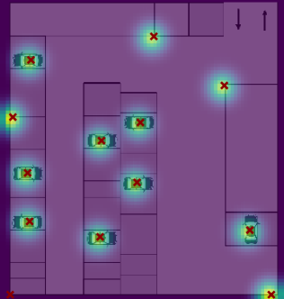
Figure 1: Collaborative auto-positioning for smart parking applications: State estimation and associated uncertainties based on probability grid mapping (purple, reference positions in red).

In addition, a strict distinction between stationary and mobile devices will not be applicable anymore due to the variant nature of many applications, where variability of the environment is a main focus and non-stationary configurations are imperatively required. While this may be regarded challenging conceptionally, these new architectures also provide the capabilities for immersive IPS and ehance their scalability.

A potential use case in the context of intelligent transportation systems (ITS) is depicted in Fig. 1 [8], where LBS for in-house parking are provided. In this example, the amount of stationary anchors can drastically be reduced by incorporating quasi-static devices representing parking cars. This use case is addressed as efficient parking is one of the main challenges for individual motorized transportation in urban areas [9]. In this context, the usage of auto-positioning enables a time- and cost-efficient roll out of IPS by dispensing positional surveying of stationary nodes. In addition, static infrastructure can be reduced as quasi-static nodes can be incorporated. This also corresponds to a variety of use cases in other application fields.

I-A Status quo of Auto-Positioning

For this task, collaborative auto-positioning, also known as self-calibration, is intended as the automatic procedure that allows anchor nodes to identify their own locations without additional interventions, e.g. manual surveying [10]. In the context of location-aware communication systems, auto-positioning can aid to increase the applicability and scalability of both device-based and device-free localization [11]. This holds true, especially for dense, location-aware networks like 5G [12, 13].

The basic idea of auto-positioning is related to collaborative localization, which has been intensively studied in the past years [14], where inter-mobiles ranges are used to support the localization process and still rely on previously surveyed locations of the reference points. A comprehensive survey and literature review of self-calibration and collaborative localization, especially emphasizing their differences and similarities is given in [10]. Theoretical works with regards to achievable performance are provided in [15], where the Cramér-Rao lower bound for auto-positioning is investigated.

A common approach to auto-positioning without any pre-surveyed anchor positions is the usage of closed-form (CF) methods as proposed in [15, 16, 17]. These methods are based on similar assumptions for auto-positioning, which will further be discussed in Section II. However, CF methods require the simultaneous incorporation of observations obtained from multiple nodes. Hence, the success rate in the presence of unknown constellations and measurement failures is limited.

A Least-Squares-Estimation (LSE) approach is used in [16] to minimize the errors between the inter-anchor measurements. The calibration of the anchors is done if a certain error threshold is exceeded. The automate coordinate formation in [17] is supplemented with a node placement strategy and an outlier removal algorithm. Ref. [18] utilizes additional calibration modules within the network in order to reduce the positional error. For this additional anchor calibration, the performance of three localization algorithms is tested via multidimensional scaling, semidefinite programming and iterative trilateration.

In order to further increase the accuracy of auto-positioning based on trilateration by means of hardware and ranging enhancements, [19] proposes an antenna delay calibration based on an Asymmetric Double-sided Two-way Ranging (ADS-TWR) scheme. Furthermore, [20] proposes two novel algorithms to improve the accuracy and success rate of auto-positioning, namely Triangle Reconstruction Algorithm (TRA) and Channel Impulse Response Positioning (CIRPos). Both algorithms, were tested in a simulated environment. With regards to technologies, most of the cited works investigated the proposed methods based on Ultra-Wideband (UWB) respectively simulation procedures.

In general, auto-positioning leads to correlated inter-node observations, whose uncertainties with respect to the position information and measurement noise need to be considered during estimation. Especially in the presence of non-line-of-sight and multipath propagation robust state estimation is required, as these error types lead to non-gaussian residual distributions, which hurt the presumptions of estimators like the LSE. The works in [21, 18, 19, 20] target the accuracy improvement of self-calibration by identifying non-line-of-sight observations, e.g. by applying machine learning.

I-B Focus and structure of this paper

This paper presents a grid-based Bayesian formulation of the collaborative auto-positioning problem for IPS. A grid-based representation was chosen in order to provide a shared state space for collaborative users and to potentially include a-priori knowledge about the environment. The presented, non-parametric filtering approach provides a robust state estimation compared to conventional CF methods for non-stationary and unknown network configurations, while lowering the requirements with regards to connectivity and availability of viable ranging measurements. To underline this, we use multipath- and outlier-corrupted simulation data aiming to provide a real-world proximate data foundation for method validation. The simulation procedure emulates UWB range measurements with respect to three different scenarios.

The rest of the paper is organized as follows: Section II describes a baseline CF auto-positioning method. The there described relations are used for initialization of the grid-based auto-positioning method, which is presented in Section III. In order to validate the proposed method, a brief introduction on the applied empirical simulation method for three different ranging residual distributions and quantitative positioning accuracy results for these scenarios are given in Section IV. The paper concludes with a summary and proposals for future research work in Section V.

II Closed-Form Auto-Positioning

The aforementioned CF methods for auto-positioning based on distance measurements are applied by meeting a variety of presumptions. In order to estimate the positions of three anchors $\boldsymbol{A}_{0}$, $\boldsymbol{A}_{1}$ and $\boldsymbol{A}_{2}$ within a network, the methods proposed in [15] and [20] formulate the following presumptions:

• $\boldsymbol{A}_{0}$ is situated at the coordinate origin;

• The direction from $\boldsymbol{A}_{0}$ to $\boldsymbol{A}_{1}$ defines the positive x-axis;

• $\boldsymbol{A}_{2}$ lies in the half-plane with positive y-coordinate;

• Extension: $\boldsymbol{A}_{3}$ lies in the positive z-direction.

A corresponding two-dimensional constellation and the provided pair-wise distance measurements $\boldsymbol{d}$ are depicted in Fig. 2. Given this frame, each anchor position $\boldsymbol{A}_{n}$ is defined as $\boldsymbol{A}_{n}=[x_{n},y_{n}]^{\intercal}$. Assuming a total of $N$-nodes, the inter-anchor distances form the square measurement matrix $\boldsymbol{D}_{t}$ at timestep $t$:

$$\boldsymbol{D}_{t}=\begin{pmatrix}d_{0,0}&d_{0,1}&\cdots&d_{0,N}\\ d_{1,0}&d_{1,1}&\cdots&d_{1,N}\\ \vdots&\vdots&\ddots&\vdots\\ d_{n,0}&d_{N,1}&\cdots&d_{N,N}\end{pmatrix}$$

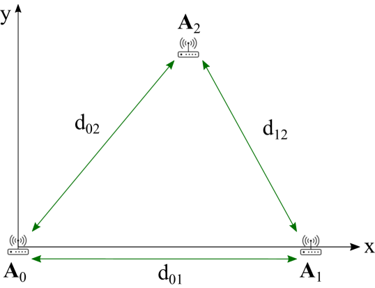
Figure 2: Configuration of network nodes $\boldsymbol{A}_{0}$ to $\boldsymbol{A}_{2}$ and their pair-wise distances $d$.

Please note, that the x-coordinate of $\boldsymbol{A}_{1}$ represents the measured distance between itself and node $\boldsymbol{A}_{0}$.

$$\boldsymbol{A}_{0} =[x_{0},y_{0}]^{\intercal}=[0,0]^{\intercal}$$ (1)

$$\boldsymbol{A}_{1} =[x_{1},y_{1}]^{\intercal}=[d_{01},0]^{\intercal}$$ (2)

$$\boldsymbol{A}_{2} =[x_{2},y_{2}]^{\intercal}=[\frac{d_{02}^{2}-d_{12}^{2}+x_{1}^{2}}{2x_{1}},\sqrt{d_{02}^{2}-x_{2}^{2}}]^{\intercal}$$ (3)

Additional nodes in the network can be calculated via Eq. 3 or estimated based on the position data of the first three nodes and their ranges to them. A detailed derivation of Eq. 3 is given in [17].

Given CF approaches, we identify two major challenges when it comes to real-world applications: Presence of corrupted measurements (multipath reception and outliers) and measurement failures. Concerning the latter, both the pair-wise distances $d_{0,1}$ between $\boldsymbol{A}_{0}$ and $\boldsymbol{A}_{1}$ and the respective ranging measurements to the node of interest $n$ $d_{0,n}$ and $d_{1,n}$ need to be available in order to estimate node positions for $n>1$. In the presence of measurement confusions, failures and nodes possibly being out of reception range, this leads to descending success rates, which we will further discuss in Section IV. In addition, CF methods as well as parametric estimators are performing poorly in the presence of non-line-of-sight (NLOS) and multipath reception as well as correlation between observations. Therefore real-world scenarios provide inherent challenges for these methods, which need to be considered.

III Bayesian Auto-Positioning Approach

In order to do so, we propose a Bayesian formulation based on a discrete grid in order to solve the auto-positioning problem. This Markov Localization recursively estimates the a-posteriori probability density function (pdf), commonly reffered to as belief or posterior, of the current state via the observation Likelihood, while incorporating process knowledge and state history via the Markov assumption and Bayes’ rule in order to provide a more robust state estimation [22]:

$$\text{posterior}\propto\text{likelihood}\times\text{prior}$$ (4)

III-A Fundamentals

The proposed method, which we will refer to as collaborative grid positioning (CGP) is based on an equidistant grid representation of the state space, which therefore represents possible realizations of the node’s location. This representation was chosen because it provides a shared and unified state space of multiple nodes while dispensing a foundation for non-parametric state estimation, which is more robust towards non-gaussian measurement noise and multi-modalities. The method is also referred to as multi-dimensional histogram filter (HF) [22], which corresponds to the point-mass filter [23].

For this method, the state space given the two-dimensional state vector $\mathcal{X}_{t}=[x_{t},y_{t}]^{\intercal}$ representing the position of a node, is decomposed in a discrete and finite set of $M$-equidistant realizations $X_{M}$:

$$\text{dom}(\boldsymbol{\mathcal{X}})=\boldsymbol{X}_{1}\cup\boldsymbol{X}_{2}\cup\dots\boldsymbol{X}_{M}$$ (5)

The general procedure for the estimation of a single node, following the well-known Recursive Bayes’ Filter structure, is given in Fig. 3, where the hidden state space vector $\boldsymbol{\mathcal{X}}_{t}$ is incrementally estimated based on the last given state $\boldsymbol{\mathcal{X}}_{t-1}$.

Figure 3: Conceptual structure of CGP.

The corresponding calculations are given as follows [22]:

$$\overline{\boldsymbol{p}}_{t} =\boldsymbol{p}_{t-1}\sum_{m}\boldsymbol{P}(\boldsymbol{\mathcal{X}}_{t,m}|{\boldsymbol{\mathcal{X}}}_{t-1})$$ (6)

$$\boldsymbol{p}_{t} =\eta\;\overline{\boldsymbol{p}}_{t}\sum_{m}\boldsymbol{P}(\mathcal{\boldsymbol{\mathcal{Z}}}_{t}|\boldsymbol{\mathcal{X}}_{t,m})$$ (7)

$$\boldsymbol{\hat{\mathcal{X}}}_{t} =\text{argmax}\;\boldsymbol{p}_{t},$$ (8)

where $\overline{\boldsymbol{p}}_{t}$ and $\boldsymbol{p}_{t}$ denote the predicted and the resulting belief, based on the observation Likelihood $\boldsymbol{P}(\mathcal{\boldsymbol{\mathcal{Z}}}_{t}|\boldsymbol{\mathcal{X}}_{t,m})$ and the normalization constant $\eta$. The resulting state estimation $\boldsymbol{\hat{\mathcal{X}}}_{t}$ is obtained from maximizing the current belief.

III-B Inter-node Likelihood calculation

In contrast to conventional radio-based localization systems, where observations are only obtained from stationary anchors, collaborative auto-positioning needs to consider and propagate the associated uncertainties about the locations of the network nodes. This also poses a major challenge in collaborative positioning scenarios [24].

In order to underline this problem, the correlation and statistical dependency is depicted in Fig. 4, which shows the correlation dependencies of inter-node observations.

Figure 4: Graphical representation of the state estimation problem based on correlated inter-node observations.

Therefore, the uncertainty of both the ranging measurements $\sigma_{r}$ as well as the uncertainties of the node estimations $\sigma_{\boldsymbol{A}_{n}}$ need to be accounted for Likelihood calculation. Given two nodes $\boldsymbol{A}_{1,2}$ and in correspondence to [25], the inter-node ranging noise is given as:

$$\sigma_{1,2}=\sigma_{r}+\sqrt{\textrm{tr}(\hat{\boldsymbol{\Sigma}}_{1})}+\sqrt{\textrm{tr}(\hat{\boldsymbol{\Sigma}}_{2})},$$ (9)

where $\textrm{tr}(\cdot)$ denotes the trace operator. The node-individual covariance matrices $\boldsymbol{\Sigma}_{n}$ can be computed as the sample variance given the previously defined state space and the calculated Likelihood for each sample by determining the weighted average:

$$\boldsymbol{\Sigma}_{n,t}\approx\sum_{m}\boldsymbol{p}_{m}(\boldsymbol{X}_{m}-\hat{\boldsymbol{\mathcal{X}}}_{n,t})^{2}$$ (10)

A graphical example of the measurement uncertainties between a conventional range measurement obtained from a stationary anchor compared to auto-positioning is given in Fig. 5.

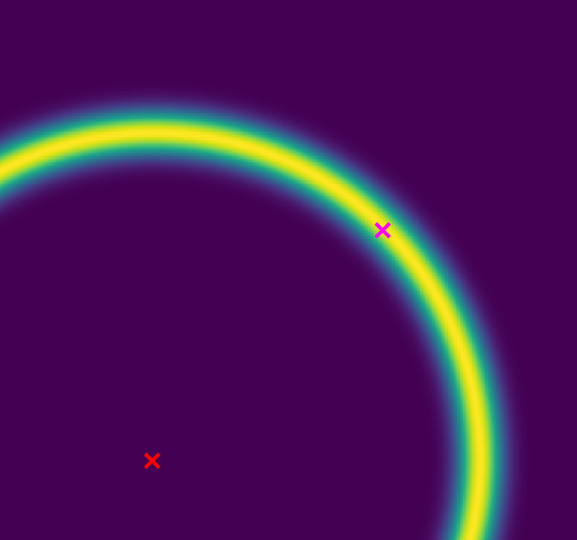
(a) Stationary

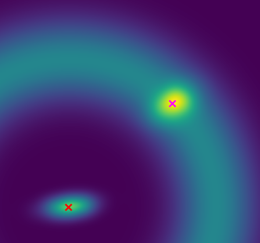
(b) Non-stationary

Figure 5: Observation variance: (a) Uncorrelated case with stationary nodes; (b) Correlated case for non-stationary nodes.

Given the auto-positioning problem at hand, the observation Likelihood based on the ranging measurement $r$ can be sampled from a normal distribution:

$$\boldsymbol{P}(\mathcal{\boldsymbol{\mathcal{Z}}}|\boldsymbol{\mathcal{X}}_{m})\leftarrow\mathcal{N}(\boldsymbol{y}_{m},\boldsymbol{\Sigma})$$ (11)

where $y$ denotes the euclidean distance residual between the observed measurement and $m$-grid-node relation:

$$\boldsymbol{y}_{m}=\left\|\boldsymbol{X}_{n}-\boldsymbol{X}_{m}\right\|_{2}-\boldsymbol{r}$$ (12)

III-C Implementational Details

The structure and a flowchart of the CGP implementation are visualized in Fig. 6. Similar to the CF, the position of $\boldsymbol{A}_{0}$ is set to the origin of the coordinate system. Next up, the position of $\boldsymbol{A}_{1}$ is estimated with the proposed CGP approach in a one-dimensional representation, depending on the availability of the ranging measurement to $\boldsymbol{A}_{0}$. This dimensional reduction corresponds to a HF and can be applied based on the presumptions formulated in Section II.

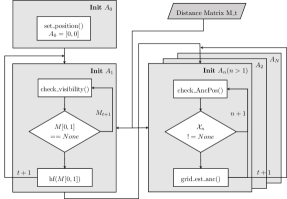
Figure 6: Flowchart of the proposed CGP auto-positioning.

In contrast to the CF, for CGP the next step is to estimate the remaining sensor node positions based on all previously estimated sensor node positions and their measured distances to the node of interest. This is done by applying the two-dimensional CPG as previously described. In order to lower the demands on the availability of observations compared to the CF approach, CGP does not require specific ranging combinations to be available (cf. Section II), which raises its robustness against measurement failures. This effect will further be discussed in Section IV. Therefore, in each estimation step, the visibility to all remaining nodes is checked and available observations in combination with the originating state estimation and associated uncertainty are taken into account.

Due to the non-parametric nature of the CGP, NLOS reception and measurement outliers are compensated to a certain extent, without the need for additional error identification and mitigation, which helps in providing an easily applicable auto-positioning approach.

IV Validation and Results

In order to assess the proposed auto-positioning method with respect to the aforementioned challenges, a semi-empirical ranging simulation procedure based on our previously published work [26] is applied. Since many high-precision positioning systems for IPS are based on the UWB technology, the simulation intends to rebuild typical error types in magnitudes with respect to IPS scenarios. The simulation procedure allows an adaptive tuning of parameters to ensure real-world proximate performance validation. The scenario of choice corresponds to the constellation depiced in Fig. 1.

IV-A Methodology

We assume that a ranging measurement $r$ comprises the true, euclidean distance between two nodes $d=\left\|\boldsymbol{A}_{1}-\boldsymbol{A}_{2}\right\|_{2}$ and additive errors following [27]:

$$r=\begin{cases}d+{\text{\char 101}}&\text{if }p>\dfrac{d}{d_{\mathrm{max}}}\\ \emptyset&\text{else.}\end{cases}$$ (13)

The additive error terms are modeled as linearly distant-dependent with respect to an empirical maximum range $d_{\text{max}}$, which can be set with regards to the application and technology at hand. If the formulated condition is not met, a measurement failure is simulated. In addition, the probability $p$ for sporadic measurement perturbations is modeled as a Bernoulli experiment with $p\sim\mathcal{U}(0,1)$. The distance dependency of errors was empirically shown in [26] and also influences the success rate of simulated measurements. Depending on this ratio, the classification of the error variable is obtained from:

$${\text{\char 101}}=\begin{cases}{\text{\char 101}}_{\mathrm{mp}}&\text{if }p_{\text{\char 101}}>0.8-0.3\dfrac{d}{d_{\mathrm{max}}},{\text{\char 101}}_{\mathrm{mp}}<d\\ {\text{\char 101}}_{\mathrm{out}}&\text{if }p_{\text{\char 101}}<p_{\mathrm{out}}\\ {\text{\char 101}}_{\mathrm{hw}}&\text{else,}\end{cases}$$ (14)

where the outlier probability $p_{\text{out}}$ is also an empirical value describing the outlier probability. Based on this classification and among the aforementioned measurement failures, three types of errors are sampled:

$${\text{\char 101}}_{\mathrm{mp}} \sim\mathcal{LN}(\overline{R}_{\mathrm{mp}},\sigma_{\mathrm{mp}}^{2})$$ (15)

$${\text{\char 101}}_{\mathrm{out}} \sim\mathcal{U}(-d,d_{\mathrm{max}}-d)$$ (16)

$${\text{\char 101}}_{\mathrm{hw}} \sim\mathcal{N}(0,\sigma_{r}^{2}).$$ (17)

${\text{\char 101}}_{\mathrm{hw}}$ represent normally distributed LOS measurements, ${\text{\char 101}}_{\mathrm{out}}$ a uniformly distributed outlier magnitude with respect to the given reference distance. Finally, ${\text{\char 101}}_{\mathrm{mp}}$ is modeled as a right-skewed log normal distribution [28], where the skewness of the log normal distribution depends on the diversity of the NLOS channel. The applied parameters and probabilities are summarized in Table I.

IV-B Ranging Simulation

In total, three different ranging distributions are simulated, where the measurement residuals for each scenario are shown in Fig. 7 and each scenario emulates different environmental conditions. In addition, Table I also contains the relative amount of LOS, NLOS, outlier and failure rates.

Given a constellation of 13 nodes (cf. Fig. 1), each scenario contains 1.000 measurement epochs and therefore approximately 13.000 estimated positions based on around 170.000 ranging measurements, allowing a statistical assessment of each constellation.

Table I: Overview of simulation parameterization for three simulation scenarios, percentage ranging simulation results and quantitative positioning performance of both CF and CGP.

		I	II	III
Parameter	PDFs	$\mathcal{N}(0,0.9)\quad\mathcal{LN}(0.8,1.07)$
	$d_{\textrm{max}}$ (m)	100	100	50
	$p_{\textrm{out}}$	0	0.07	0.20
	NLOS (%)	0	0.21	0.20
Simulation	LOS (%)	1	0.61	0.56
	NLOS (%)	0	0.21	0.20
	Outlier (%)	0	0.06	0.15
	Failures (%)	0	0.12	0.09
CF	RMSE (m)	0.41	3.80	6.99
	1-$\sigma$ (m)	0.51	2.06	4.01
	2-$\sigma$ (m)	0.93	19.41	37.25
	3-$\sigma$ (m)	1.25	47.22	62.93
	Succes (%)	1	0.37	0.36
CGP	RMSE (m)	0.17	0.42	0.93
	1-$\sigma$ (m)	0.28	0.50	1.43
	2-$\sigma$ (m)	0.36	0.58	1.57
	3-$\sigma$ (m)	0.44	0.59	1.58
	Succes (%)	1	1	1

Scenario I corresponds to exclusively gaussian noise representing only LOS measurements. Additionally, scenario II incorporates multipath errors, outliers and measurement failures. Finally, scenario III puts even more emphasis on occurring outliers.

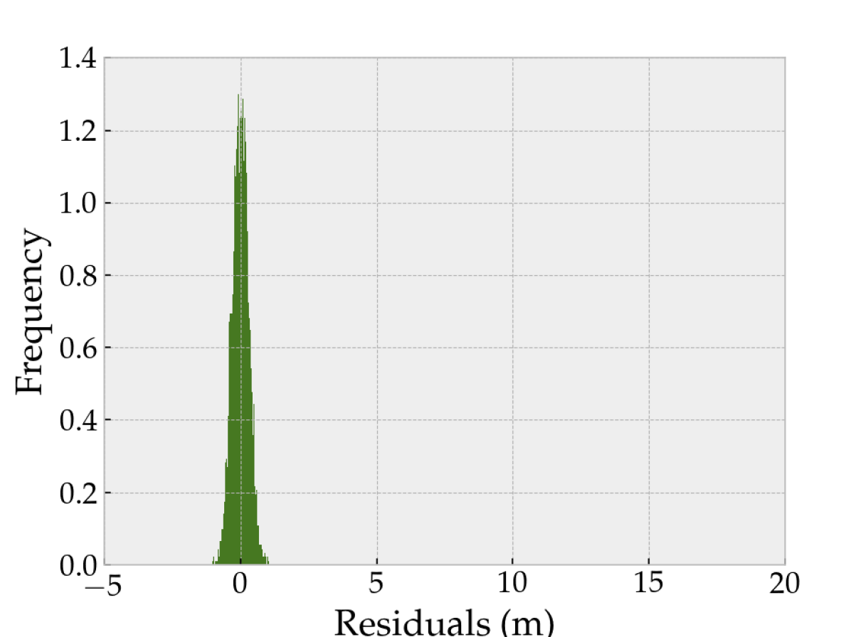
(a) I

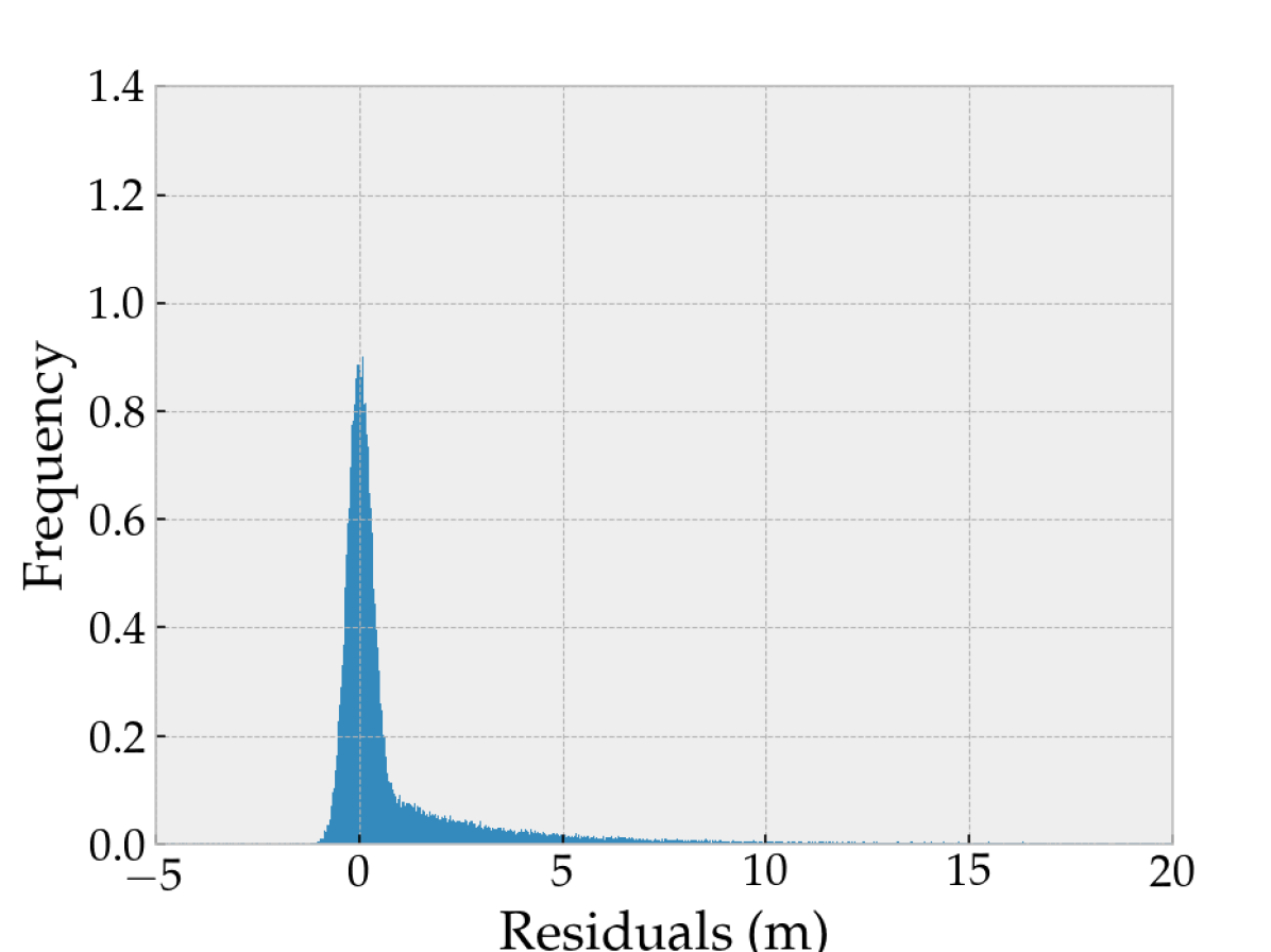
(b) II

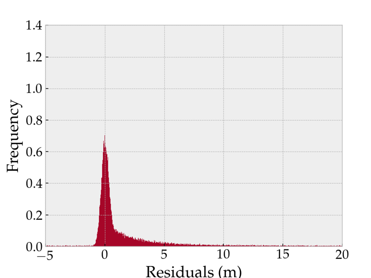
(c) III

Figure 7: Histogram of ranging residual PDFs for the examined scenarios. Simulation parameters are included in Table I.

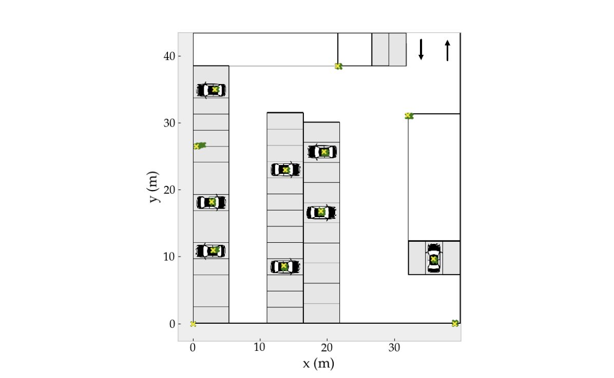
(a) I

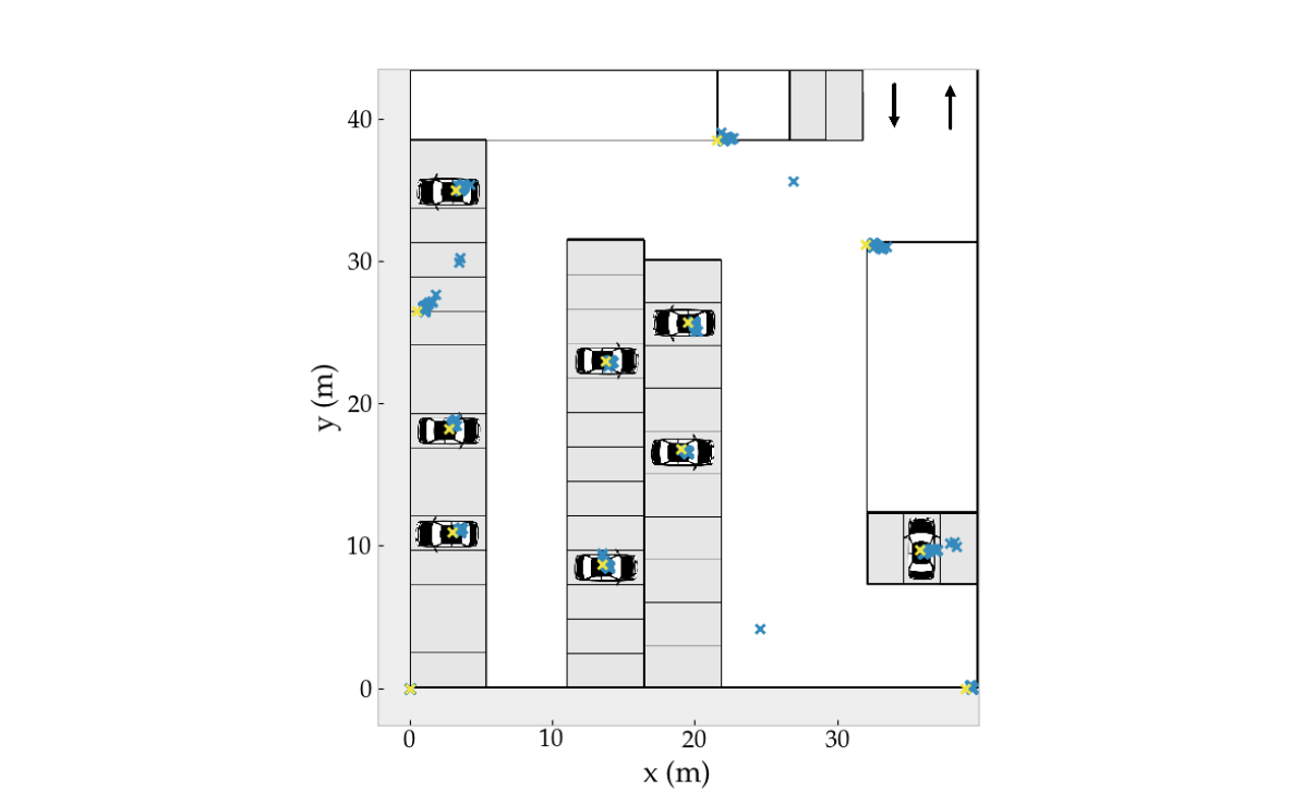
(b) II

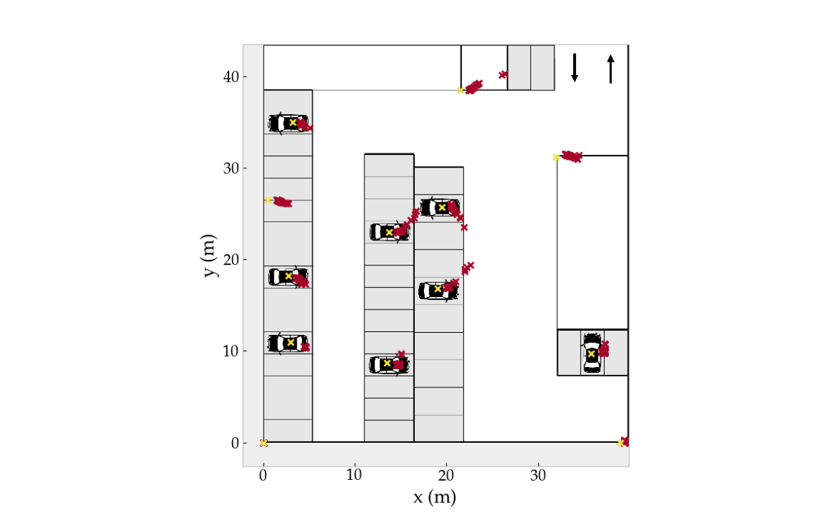
(c) III

Figure 8: Qualitative results of CGP position estimation based on the previously presented residual PDFs (cf. Fig. 7) including the references (yellow) and estimated node positions (green, blue, red).

IV-C Positioning Performance

In this subsection we provide performance results of the proposed CGP approach in comparison to the aforementioned CF method and with respect to the previously introduced ranging residual distributions (cf. Fig. 7). The qualitative results for each distribution are shown in Fig. 8. In addition, the individual root mean square errors (RMSE) and error quantiles for both CGP and CF are detailed in Table I. A graphical presentation of quantitative results is also given in Fig. 9, which depicts the empirical cumulative distribution functions (ECDFs) for both the CGP and the CF methods and simulation scenarios.

As expected, scenario I achieves the most accurate position estimates. The underlying gaussian distribution contains no multipath effects, outliers and observation failures so that the ECDFs of both methods converges quickly (cf. Fig. 9) and reveals a RMSE of $0.41\text{\,}\mathrm{m}$ respectively $0.17\text{\,}\mathrm{m}$ for CF and CGP with a $3-\sigma$ error quantile ($99,73\%$) of $1.25\text{\,}\mathrm{m}$ and $0.44\text{\,}\mathrm{m}$.

The results based on data sets II and III which entail multipath errors ${\text{\char 101}}_{\mathrm{mp}}$ about 20% as well as different amounts of outliers and failures, are qualitatively shown in Figs. 8(b) and 8(c). Again, the proposed CGP method outperforms the baseline CF approach in terms of accuracy. This is also underlined in Fig. 9.

Next to the resulting accuracy, we want to emphasize the advantages of CGP compared to CF with regards to success rate. For both scenario II and III, the overall CF success rate is around 0.36%. Due to the restrictions of observation availability, the success rate drastically decreases.

For the introduced use case of location-aware smart parking applications, III reveals that, even in the presence of 15% outliers and 0.09% measurement failures, a $3-\sigma$ accuracy of $1.58\text{\,}\mathrm{m}$ was achieved, which corresponds to a parking lot selective positioning accuracy.

V Conclusion

In this paper, the research topic of auto-positioning for radio-based localization systems in non-static configurations was addressed. In general, auto-positioning aims to both provide position estimation of stationary anchors without time-consuming position surveying, as well as being to able to be seamlessly integrated in non-stationary network configurations. In this context, a novel approach of auto-positioning for node self-calibration, intended to provide robust state estimation in the presence of NLOS reception, ourliers and measurement failures, was presented.

This is achieved by extending previously CF methods with a non-parametric, grid-based formulation, which we referred to as CGP. In order to emphasize the advantages of CGP in comparison with CF methods, we discussed and described three different ranging residual distributions, which correspond to different environmental and reception scenarios and are characterized by distinct error occurrence probabilities and magnitudes.

Based on this, we empirically showed, that the proposed CGP method was able to outperform the baseline CF approach both in terms of node positioning accuracy and success rate, due to the robust formulation as well as imposing fewer requirements for network connectivity and availability of ranging measurements.

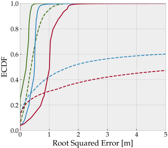
Figure 9: ECDFs for all scenarios (CGP solid, CF dotted).

References

- [1] C. Laoudias, A. Moreira, S. Kim, S. Lee, L. Wirola, and C. Fischione, “A survey of enabling technologies for network localization, tracking, and navigation,” IEEE Communications Surveys & Tutorials, vol. 20, no. 4, pp. 3607–3644, 2018. [Online]. Available: https://doi.org/10.1109/comst.2018.2855063
- [2] J. A. Zhang, M. L. Rahman, K. Wu, X. Huang, Y. J. Guo, S. Chen, and J. Yuan, “Enabling joint communication and radar sensing in mobile networks—a survey,” IEEE Communications Surveys & Tutorials, vol. 24, no. 1, pp. 306–345, 2022. [Online]. Available: https://doi.org/10.1109/comst.2021.3122519
- [3] K. Shafique, B. A. Khawaja, F. Sabir, S. Qazi, and M. Mustaqim, “Internet of things (IoT) for next-generation smart systems: A review of current challenges, future trends and prospects for emerging 5g-IoT scenarios,” IEEE Access, vol. 8, pp. 23 022–23 040, 2020. [Online]. Available: https://doi.org/10.1109/access.2020.2970118
- [4] A. Bourdoux, A. N. Barreto, B. van Liempd, C. de Lima, D. Dardari, D. Belot, E.-S. Lohan, G. Seco-Granados, H. Sarieddeen, H. Wymeersch, J. Suutala, J. Saloranta, M. Guillaud, M. Isomursu, M. Valkama, M. R. K. Aziz, R. Berkvens, T. Sanguanpuak, T. Svensson, and Y. Miao, “6G White Paper on Localization and Sensing,” ArXiv, 2020. [Online]. Available: http://arxiv.org/abs/2006.01779
- [5] G. M. Mendoza-Silva, J. Torres-Sospedra, and J. Huerta, “A meta-review of indoor positioning systems,” Sensors, vol. 19, no. 20, p. 4507, 10 2019. [Online]. Available: https://doi.org/10.3390/s19204507
- [6] X. Li, Y. Cui, J. A. Zhang, F. Liu, X. Jing, and O. A. Dobre, “Assisting living by wireless sensing: The role of integrated sensing and communications in 6g era,” 2022. [Online]. Available: https://arxiv.org/abs/2202.09522
- [7] F. Zafari, A. Gkelias, and K. K. Leung, “A survey of indoor localization systems and technologies,” IEEE Communications Surveys Tutorials, vol. 21, no. 3, pp. 2568–2599, 2019.
- [8] A. Jung., P. Schwarzbach., and O. Michler., “Future parking applications: Wireless sensor network positioning for highly automated in-house parking,” in Proceedings of the 17th International Conference on Informatics in Control, Automation and Robotics - ICINCO,, INSTICC. SciTePress, 2020, pp. 710–717.
- [9] J. Ninnemann, P. Schwarzbach, and O. Michler, “Multipath-assisted Radio Sensing and Occupancy Detection for Smart In-house Parking in ITS,” in 2021 International Conference on Indoor Positioning and Indoor Navigation (IPIN), 2022.
- [10] M. Ridolfi, A. Kaya, R. Berkvens, M. Weyn, W. Joseph, and E. D. Poorter, “Self-calibration and collaborative localization for uwb positioning systems: A survey and future research directions,” ACM Comput. Surv., vol. 54, no. 4, may 2021. [Online]. Available: https://doi.org/10.1145/3448303
- [11] A. Liu, Z. Huang, M. Li, Y. Wan, W. Li, T. X. Han, C. Liu, R. Du, D. K. P. Tan, J. Lu, Y. Shen, F. Colone, and K. Chetty, “A survey on fundamental limits of integrated sensing and communication,” IEEE Communications Surveys & Tutorials, pp. 1–1, 2022. [Online]. Available: https://doi.org/10.1109/comst.2022.3149272
- [12] A. Hakkarainen, J. Werner, M. Costa, K. Leppanen, and M. Valkama, “High-efficiency device localization in 5g ultra-dense networks: Prospects and enabling technologies,” in 2015 IEEE 82nd Vehicular Technology Conference (VTC2015-Fall). IEEE, Sep. 2015. [Online]. Available: https://doi.org/10.1109/vtcfall.2015.7390965
- [13] H. Kim, K. Granstrom, L. Gao, G. Battistelli, S. Kim, and H. Wymeersch, “5g mmWave cooperative positioning and mapping using multi-model PHD filter and map fusion,” IEEE Transactions on Wireless Communications, vol. 19, no. 6, pp. 3782–3795, Jun. 2020. [Online]. Available: https://doi.org/10.1109/twc.2020.2978479
- [14] N. Chukhno, S. Trilles, J. Torres-Sospedra, A. Iera, and G. Araniti, “D2d-based cooperative positioning paradigm for future wireless systems: A survey,” IEEE Sensors Journal, vol. 22, no. 6, pp. 5101–5112, Mar. 2022. [Online]. Available: https://doi.org/10.1109/jsen.2021.3096730
- [15] M. Hamer and R. D’Andrea, “Self-calibrating ultra-wideband network supporting multi-robot localization,” IEEE Access, vol. 6, pp. 22 292–22 304, 2018.
- [16] C. M. Almansa, W. Shule, J. P. Queralta, and T. Westerlund, “Autocalibration of a mobile uwb localization system for ad-hoc multi-robot deployments in gnss-denied environments,” 2020. [Online]. Available: https://arxiv.org/abs/2004.06762
- [17] P. Loahavilai, C. Thanapirom, P. Rattanawan, T. Chulapakorn, S. Yanwicharaporn, C. Kingkan, K. Prasertsuk, and N. Cota, “Rapid deployment of ultra-wideband indoor positioning system,” in 2021 18th International Joint Conference on Computer Science and Software Engineering (JCSSE), 2021, pp. 1–6.
- [18] P. Krapež and M. Munih, “Anchor calibration for real-time-measurement localization systems,” IEEE Transactions on Instrumentation and Measurement, vol. 69, no. 12, pp. 9907–9917, 2020.
- [19] C. Phoojaroenchanachai, C. Suwatthikul, K. Maneerat, K. Hormsup, K. Chinda, S. Wisadsud, T. Demeechai, L. Kovavisaruch, and K. Kaemarungsi, “An extendable auto-position for uwb-based indoor positioning systems,” in 2021 25th International Computer Science and Engineering Conference (ICSEC), 2021, pp. 334–339.
- [20] J. Pereira, “Anchor self-calibrating schemes for uwb based indoor localization,” Ph.D. dissertation, Rochester Institute of Technology, 2021.
- [21] M. Ridolfi, J. Fontaine, B. Van Herbruggen, W. Joseph, J. Hoebeke, and E. De Poorter, “Uwb anchor nodes self-calibration in nlos conditions: a machine learning and adaptive phy error correction approach,” Wireless Networks, vol. 27, 05 2021.
- [22] S. Thrun, W. Burgard, and D. Fox, Probabilistic Robotics (Intelligent Robotics and Autonomous Agents). The MIT Press, 2005.
- [23] R. Bucy and K. Senne, “Digital synthesis of non-linear filters,” Automatica, vol. 7, no. 3, pp. 287–298, May 1971. [Online]. Available: https://doi.org/10.1016/0005-1098(71)90121-x
- [24] A. Minetto, A. Gurrieri, and F. Dovis, “A cognitive particle filter for collaborative DGNSS positioning,” IEEE Access, vol. 8, pp. 194 765–194 779, 2020. [Online]. Available: https://doi.org/10.1109/access.2020.3033626
- [25] D. Medina, L. Grundhofer, and N. Hehenkamp, “Evaluation of estimators for hybrid GNSS-terrestrial localization in collaborative networks,” in 2020 IEEE 23rd International Conference on Intelligent Transportation Systems (ITSC). IEEE, Sep. 2020. [Online]. Available: https://doi.org/10.1109/itsc45102.2020.9294750
- [26] P. Schwarzbach, R. Weber, and O. Michler, “Statistical evaluation and synthetic generation of ultra-wideband distance measurements for indoor positioning systems,” IEEE Sensors Journal, vol. 22, no. 6, pp. 4836–4843, Mar. 2022. [Online]. Available: https://doi.org/10.1109/jsen.2021.3121627
- [27] Y. Qi, H. Kobayashi, and H. Suda, “Analysis of wireless geolocation in a non-line-of-sight environment,” IEEE Transactions on wireless communications, vol. 5, no. 3, pp. 672–681, 2006.
- [28] A. Prorok, P. Tomé, and A. Martinoli, “Accommodation of nlos for ultra-wideband tdoa localization in single- and multi-robot systems,” in 2011 International Conference on Indoor Positioning and Indoor Navigation, 2011, pp. 1–9.