A conforming auxiliary space preconditioner for the mass conserving mixed stress method

Abstract.

We are studying the efficient solution of the system of linear equation stemming from the mass conserving mixed stress (MCS) method discretization of the Stokes equations. To that end we perform static condensation to arrive at a system for the pressure and velocity unknowns. An auxiliary space preconditioner for the positive definite velocity block makes use of efficient and scalable solvers for conforming Finite Element spaces of low order and is analyzed with emphasis placed on the polynomial degree of the discretization. Numerical experiments demonstrate the potential of this approach and the efficiency of the implementation.

1. Introduction

Let $\Omega\subset\mathbb{R}^{d}$ be a bounded domain with $d=2$ or $3$ with Lipschitz boundary $\Gamma\mathrel{\mathop{\mathchar 58\relax}}=\partial\Omega$. Let $u$ and $p$ be the velocity and the pressure, respectively. Given an external body force $f\mathrel{\mathop{\mathchar 58\relax}}\Omega\to\mathbb{R}^{d}$ and the double of kinematic viscosity denoted by ${\nu}$, the velocity-pressure formulation of the Stokes system is given by

(1a) $$-\operatorname{div}({\nu}{\varepsilon}(u))+\nabla p =f\quad\textrm{in }\Omega,$$

(1b) $$\operatorname{div}(u) =0\quad\textrm{in }\Omega,$$

where ${\varepsilon}({{u}})=\frac{1}{2}(\nabla u+(\nabla u)^{{T}})$. By introducing additional matrix valued variables $\sigma\mathrel{\mathop{\mathchar 58\relax}}=-\nu{\varepsilon}(u)$ for the stress and $\omega\mathrel{\mathop{\mathchar 58\relax}}=\frac{1}{2}(\nabla u-(\nabla u)^{T})$, these equations can be restated as

(2a) $$-\nu^{-1}\operatorname{dev}{(\sigma)}-\nabla u+\omega =0\quad\textrm{in }\Omega,$$

(2b) $$\operatorname{div}(\sigma)+\nabla p =f\quad\textrm{in }\Omega,$$

(2c) $$\sigma-\sigma^{{T}} =0\quad\textrm{in }\Omega,$$

(2d) $$\operatorname{div}(u) =0\quad\textrm{in }\Omega,$$

where (2a) is motivated by the fact that for the solution of (1) we have $$\sigma=-\nu{\varepsilon}(u)=-\nu\operatorname{dev}{({\varepsilon}(u))}=\operatorname{dev}{(\sigma)} \omega u$$. The introduction of as a Lagrange multiplier enables the derivation of discrete methods that enforce the symmetry constraint (2c) weakly, see also [37, 17, 6]. As boundary conditions, we consider Dirichlet ones for the velocity , homogenous purely for clarity of the presentation, and two kinds of outlet conditions,

(2e) $$u =0\quad\textrm{on }\Gamma_{D},$$

(2f) $$(\sigma+pI)n =0\quad\textrm{on }\Gamma_{N},$$

(2g) $$((\sigma+pI)n)\cdot n=u_{t} =0\quad\textrm{on }\Gamma_{\tilde{N}},$$

where $I$ is the $d\times d$ identity matrix and $u_{t}$ is the tangential part of $u$. We assume that both $\Gamma_{D}$ and at least one of $\Gamma_{N}$ or $\Gamma_{\tilde{N}}$ have positive measure. As usual, when $\Gamma_{N}=\Gamma_{\tilde{N}}=\emptyset$, an additional condition must be imposed on the pressure to make it unique.

In recent years, divergence-free and pressure-robust Finite Element discretizations, that is those whose solutions fulfill (2d) strongly, and allow for pressure-independent a-priori error estimates respectively, have been of great interest [27].

For the velocity-pressure formulation (1), one class of such methods are certain Hybrid Discontinuous Galerkin (HDG) methods that take the velocity in $H(\operatorname{div},\Omega)$ and the pressure in $L^{2}(\Omega)$, i.e. they only build normal continuity into the Finite Element space while the tangential continuity of the solution is enforced via Lagrange parameters. To make the resulting system for the velocity positive definite, a consistent stabilization term has to be added, often involving either a parameter that has to be sufficiently large or a lifting of the jump, see [36, 5].

In [30, 25], the authors presented a novel variational formulation for the Stokes equations that still takes the velocity in $H(\operatorname{div},\Omega)$ and pressure in $L^{2}(\Omega)$, remaining the property of exactly divergence-free and pressure-robust solutions, but is based on (2) instead of (1). This mass conserving mixed stress (MCS) method features a normal-tangential continuous stress space and requires no stabilizing term. It was already remarked in the original work [30] that static condensation can be performed to eliminate certain $\sigma$ degrees of freedom (dofs) and later in [26] this approach was taken to it’s logical conclusion of breaking the normal-tangential continuity of $\sigma$ with a Lagrange parameter and eliminating $\sigma$ entirely. The resulting, condense, system is one for the velocity in $H(\operatorname{div},\Omega)$, the pressure in $L^{2}(\Omega)$, and the newly introduced Lagrange parameter $\hat{u}$; It turns out to be an approximation to the tangential velocity trace on the mesh facets. The velocity unknowns $u,\hat{u}$ take the place of $\sigma$ as primal variables in the condense saddle point system, with the pressure remaining the Lagrange parameter enforcing (2d). That is, the condense system involves the same variables, and has the same structure as the HDG methods mentioned above, but without the need for a stabilization term. As the first contribution of this work we take a closer look at the condense system and in particular proof that the velocity block is in fact positive definite, as was claimed in [26] for a low order MCS method, and is related to the velocity block stemming from an HDG method with optimal stabilization.

We then move on to the question of how to efficiently solve the condense system and consider preconditioned Krylov space methods. Preconditioning techniques for saddle point systems based on separate preconditioners for the primal (velocity) and Lagrange (pressure) unknowns are a well studied subject, see [9], and the pressure Schur complement is easily preconditioned, see [40]. Therefore, our focus is on identifying and analyzing suitable preconditioners for the condense velocity block.

The literature on preconditioners for conforming methods is vast and includes, among others, domain decomposition, see [38], as well as Geometric, see [13], and Algebraic, see [43], Multigrid methods and an even somewhat comprehensive review would be beyond the scope of this work. We will take as given that efficient and scalable solvers for conforming methods exist and are available.

Preconditioners for HDG methods are not quite as well studied in literature, one recurring theme is the attempt to reuse conforming preconditioners for these non-conforming spaces. For example, a non-nested Multigrid method with conforming coarse grid spaces was studied in [16], and auxiliary space preconditioners (ASP, see [41]) that also feature a conforming sub-space were considered in [23].

The idea at the heart of both approaches is to decompose functions in the non-conforming space into a conforming component plus a (small) remainder and to address them separately with some pre-existing conforming preconditioner and a simple, computationally inexpensive method such as (Block-)Jacobi, respectively.

The principal focus in this work is on the introduction and analysis of ASPs for the MCS method. The main improvement over the theory in [23] is that the analysis of the velocity preconditioners extends techniques from [34] and is explicit in the polynomial degree of the discretization. In particular, the main result, Theorem 3, states that the condition number of a particular ASP is bounded by $\gamma\cdot(\log(k))^{3}$, where ${k}$ is the polynomial degree of the discretization and $\gamma$ is a constant stemming from the relation between condense MCS and HDG norms.

We close out the discussion with numerical experiments that demonstrate the robustness and scalability of the proposed preconditioners. It is a testament to the elegance and simplicity of the ASP method that we were able to scale the computations to a relatively large scale by leveraging existing, scalable and highly performant software.

Outline

We gather notation used throughout this work in Section 2 and introduce various Finite Element spaces and norms in Section 3 which also contains some useful technical results. Section 4 reviews the MCS method itself and contains a thorough discussion of static condensation as well as results on the obtained condense systems. Approaches for preconditioning saddle point matrices with separate preconditioners for the primal unknowns and Lagrange multipliers as well as the method of auxiliary space preconditioning are recalled in Section 5. The main results can be found in Section 6, where different variations of ASPs for the velocity block of the Stokes system are discussed. In Section 7, we sketch the treatment of the lowest order case which is not covered by the theory developed in previous sections. Finally, numerical experiments are performed in Section 8.

2. Notation

With ${\mathbb{M}}$ denoting the vector space of real $d\times d$ matrices, we define the subsets of skew-symmetric and skew-symmetric trace-free matrices by

$${\mathbb{K}}=\{\tau\in{\mathbb{M}}\mathrel{\mathop{\mathchar 58\relax}}\tau+\tau^{{T}}=0\}\quad\textrm{and}\quad{\mathbb{D}}=\{\tau\in{\mathbb{M}}\mathrel{\mathop{\mathchar 58\relax}}\tau\mathrel{\mathop{\mathchar 58\relax}}I=0\},$$

where $(\cdot)^{{T}}$ denotes the transpose and $I\in{\mathbb{M}}$ the identity matrix. To differentiate between scalar-, vector- and matrix-valued functions on some subset $D\subseteq\Omega$ we include the range in the notation for the latter two while we omit it for the former one, i.e. where $L^{2}(D,\mathbb{R})=L^{2}(D)$ denotes the space of square integrable $\mathbb{R}$-valued scalar functions, the spaces $L^{2}(D,\mathbb{R}^{d})$ and $L^{2}(D,{\mathbb{M}})$ denote the analogous vector- and matrix-valued spaces. Similarly, ${\mathbb{P}}^{{k}}(D,\mathbb{R})={\mathbb{P}}^{k}(D)$, etc., denote the set of scalar-, vector- or matrix- valued polynomials up to degree ${k}$ on $D$. We use the notation $(\cdot,\cdot)_{D}$ for the $L^{2}$-inner product on $D$ and set $\|\cdot\|^{2}_{D}=(\cdot,\cdot)_{D}$. The $L^{2}$-orthogonal projection onto ${\mathbb{P}}^{{k}}(D,\cdot)$ (the range should be clear from context) is denoted by $\Pi^{{k}}_{D}$ and we will occasionally omit the subscript. Similarly, the $L^{2}$-orthogonal projector onto the (restrictions to $D$ of) the rigid body modes $R_{D}\mathrel{\mathop{\mathchar 58\relax}}=\{u(x)=a+b\times x\mathrel{\mathop{\mathchar 58\relax}}a,b\in\mathbb{R}^{d}\}$ is written as $\Pi^{R}_{D}$.

In the following, let $\phi$, $\Phi$, and $\Psi$ be smooth scalar-, vector-, and matrix-valued functions, respectively. The operator $\nabla$ is to be understood from context as resulting in either in a vector whose components are $\partial_{i}\phi\mathrel{\mathop{\mathchar 58\relax}}=\partial\phi/\partial x_{i}$ or a matrix with components $(\partial_{i}\Phi_{j})$. For vector-valued functions in three dimensions the operator $\operatorname{curl}$ is defined as $\operatorname{curl}\Phi\mathrel{\mathop{\mathchar 58\relax}}=\nabla\times\Phi$ and in two we understand it to refer to the scalar-valued $\operatorname{curl}\phi\mathrel{\mathop{\mathchar 58\relax}}=-\partial_{2}\phi_{1}+\partial_{1}\phi_{2}$. The divergence operator $\operatorname{div}$ is understood as $\operatorname{div}\Phi\mathrel{\mathop{\mathchar 58\relax}}=\sum_{j=1}^{d}\partial_{j}\Phi_{j}$ for vectors and is applied row-wise to matrices, i.e. $(\operatorname{div}\Psi)_{i}\mathrel{\mathop{\mathchar 58\relax}}=\sum_{j=1}^{d}\partial_{j}\Psi_{ij}$. Besides the well known trace operator $\textrm{tr}({\Psi})\mathrel{\mathop{\mathchar 58\relax}}=\sum_{j=1}^{d}\Psi_{ii}$ and the deviatoric part $\operatorname{dev}{(\Psi)}\mathrel{\mathop{\mathchar 58\relax}}=\Psi-\frac{1}{d}\textrm{tr}({\Psi})I$ we further introduce the operator $\kappa\mathrel{\mathop{\mathchar 58\relax}}\mathbb{R}^{d(d-1)/2}\to{\mathbb{K}}$ by

$$\kappa(\phi)\mathrel{\mathop{\mathchar 58\relax}}=\frac{1}{2}\begin{pmatrix}0&-\phi\\ \phi&0\end{pmatrix}\;\text{ if }d=2,\qquad\kappa(\Phi)\mathrel{\mathop{\mathchar 58\relax}}=\frac{1}{2}\begin{pmatrix}0&-\Phi_{3}&\Phi_{2}\\ \Phi_{3}&0&-\Phi_{1}\\ -\Phi_{2}&\Phi_{1}&0\end{pmatrix}\;\text{ if }d=3.$$

Based on these differential operators, we use standard notation for the Sobolev spaces $H^{m}(\Omega,\mathbb{R})=H^{m}(\Omega),H(\operatorname{div},\Omega)$ and $H(\operatorname{curl},\Omega)$ with $m\geq 0$. Further, for some $\Gamma_{*}\subseteq\partial\Omega$, a subscript ”$0,\Gamma_{*}$” indicates that the corresponding natural traces vanish on $\Gamma_{*}$, and we use only the zero subscript if $\Gamma_{*}=\partial\Omega$.

We denote by $\mathcal{T}_{h}$ a quasi-uniform and shape regular triangulation of the domain $\Omega$ into tetrahedra. Let $h$ denote the maximum of the diameters of all elements in $\mathcal{T}_{h}$. The set of element interfaces and boundaries, or facets, is denoted by $\mathcal{F}_{h}$ and the set of facets of a particular element $T\in\mathcal{T}_{h}$ is $\mathcal{F}_{T}\mathrel{\mathop{\mathchar 58\relax}}=\{F\in\mathcal{F}_{h}\mathrel{\mathop{\mathchar 58\relax}}F\subseteq\partial T\}$. By an abuse of notation, we shall also use $\mathcal{F}_{h}$ to denote the domain formed by union of all $F\in\mathcal{F}_{h}$. We assume that the mesh resolves the domain boundary parts in the sense that $\forall F\in\mathcal{F}_{h}$ with $F\subseteq\partial\Omega~{}\exists!\Gamma_{*}\in\{\Gamma_{D},\Gamma_{N},\Gamma_{\tilde{N}}\}$ such that $F\subseteq\Gamma_{*}$. This splits $\mathcal{F}_{h}$ into boundary facets $\mathcal{F}_{h}^{\scriptscriptstyle D}\mathrel{\mathop{\mathchar 58\relax}}=\{F\in\mathcal{F}_{h}\mathrel{\mathop{\mathchar 58\relax}}F\subseteq\Gamma_{D}\}$, $\mathcal{F}_{h}^{\scriptscriptstyle N}\mathrel{\mathop{\mathchar 58\relax}}=\{F\in\mathcal{F}_{h}\mathrel{\mathop{\mathchar 58\relax}}F\subseteq\Gamma_{N}\}$, and $\mathcal{F}_{h}^{\scriptscriptstyle\tilde{N}}\mathrel{\mathop{\mathchar 58\relax}}=\{F\in\mathcal{F}_{h}\mathrel{\mathop{\mathchar 58\relax}}F\subseteq\Gamma_{\tilde{N}}\}$, and interior facets $\mathcal{F}_{h}^{0}\mathrel{\mathop{\mathchar 58\relax}}=\mathcal{F}_{h}\setminus(\mathcal{F}_{h}^{\scriptscriptstyle D}\cup\mathcal{F}_{h}^{\scriptscriptstyle N}\cup\mathcal{F}_{h}^{\scriptscriptstyle\tilde{N}})$. According to this mesh we also introduce the “broken” spaces

$$H^{m}(\mathcal{T}_{h},\cdot)\mathrel{\mathop{\mathchar 58\relax}}=\prod_{T\in\mathcal{T}_{h}}H^{m}(T,\cdot),\quad{\mathbb{P}}^{{k}}(\mathcal{T}_{h},\cdot)\mathrel{\mathop{\mathchar 58\relax}}=\prod_{T\in\mathcal{T}_{h}}{\mathbb{P}}^{{k}}(T,\cdot),\quad{\mathbb{P}}^{{k}}(\mathcal{F}_{h},\cdot)\mathrel{\mathop{\mathchar 58\relax}}=\prod_{F\in\mathcal{F}_{h}}{\mathbb{P}}^{{k}}(F,\cdot),$$

where, as before, we include the range explicitly e.g. as in ${\mathbb{P}}^{{k}}(\mathcal{T}_{h},\mathbb{R}^{d})$. On each $F\in\mathcal{F}_{h}$ we denote by ${[\![\cdot]\!]}$ and ${\{\!\{\cdot\}\!\}}$ the standard jump and mean value operators and take them to be the identity on boundary facets. On each element boundary and each facet $F\in\mathcal{F}_{h}$ we denote by $n$ the outward unit normal vector. The scalar normal and vector-valued tangential traces of a sufficiently smooth function $v$ are given by $v_{n}\mathrel{\mathop{\mathchar 58\relax}}=v\cdot n$ and $v_{t}\mathrel{\mathop{\mathchar 58\relax}}=v-v_{n}n$. Similarly, the normal-normal and normal-tangential traces of a smooth matrix-valued function $\Psi$ are $\Psi_{nn}\mathrel{\mathop{\mathchar 58\relax}}=\Psi\mathrel{\mathop{\mathchar 58\relax}}(n\otimes n)=n^{{{T}}}\Psi n$ and $\Psi_{nt}=\Psi n-\Psi_{nn}n$.

We write functions in general Sobolev spaces as $u,\hat{u},\omega$, etc., discrete functions with a subscript $h$ as $u_{h},\hat{u}_{h},\omega_{h}$, etc., and their via Galerkin isomorphism identified coefficient vectors w.r.t to some given Finite Element basis as $\bm{u},\hat{\bm{u}},\bm{\omega}$, etc. For readability of the presentation we make no difference between row and column vectors and, for example, write $(\bm{u},\bm{\hat{u}})$ for the coefficient vector of $(u_{h},\hat{u}_{h})$ which should strictly speaking be the column vector $(\bm{u}^{T},\bm{\hat{u}}^{T})^{T}$. Similarly, operators are capital letters $A,B$, etc., their discrete counterparts $A_{h},B_{h}$, etc., and the corresponding Finite Element matrices $\bm{A},\bm{B}$, etc. Occasionally, when it is useful to emphasize the Galerkin isomorphism we use $\sim_{\scriptscriptstyle\text{G}}$, e.g. $u_{h}\sim_{\scriptscriptstyle\text{G}}\bm{u}$ or $A_{h}\sim_{\scriptscriptstyle\text{G}}\bm{A}$.

Finally, throughout this work we write $A\lesssim B$ when there exists a constant $c>0$ independent of the mesh size $h$ and the viscosity $\nu$ such that $cA\leq B$ and $A\sim B\Leftrightarrow A\lesssim B\wedge B\lesssim A$. For example, due to quasi-uniformity we have $h\sim\textrm{diam}(T)~{}\forall T\in\mathcal{T}_{h}$. For two elliptic operators $A,B$ (or symmetric and positive definite matrices $\bm{A},\bm{B}$) we take $A\lesssim B$ to mean that the maximum eigenvalue of the generalized eigenvalue problem $Ax=\lambda Bx$ is bounded by a constant $C$ similarly independent of $h$ and $\nu$. Note that in inequalities related to discrete functions or operators, unless explicitly stated otherwise, these constants can depend on the polynomial degree. Henceforth we assume that $\nu$ is a constant.

3. Finite Elements and norm equivalences

Reminding ourselfs that the lowest order case is addressed separately in Section 7, we define the following approximation spaces for ${k}\geq 2$:

(3) $$V_{h} \mathrel{\mathop{\mathchar 58\relax}}=\{u_{h}\in{\textrm{BDM}}^{{k}}(\mathcal{T}_{h})\mathrel{\mathop{\mathchar 58\relax}}(u_{h})_{n}=0\textrm{ on }\Gamma_{D}\},$$

(4) $$\hat{V}_{h} \mathrel{\mathop{\mathchar 58\relax}}=\{\hat{u}_{h}\in{\mathbb{P}}^{{k}-1}(\mathcal{F}_{h},\mathbb{R}^{d})\mathrel{\mathop{\mathchar 58\relax}}(\hat{u}_{h})_{n}=0~{}\forall F\in\mathcal{F}_{h}\textrm{ and }\hat{u}_{h}=0~{}\forall F\subset\Gamma_{D}\cup\Gamma_{\tilde{N}}\},$$

(5) $$W_{h} \mathrel{\mathop{\mathchar 58\relax}}={\mathbb{P}}^{{k}-1}(\mathcal{T}_{h},{\mathbb{K}}),$$

(6) $$\Sigma_{h} \mathrel{\mathop{\mathchar 58\relax}}=\{\tau_{h}\in{\mathbb{P}}^{{k}}(\mathcal{T}_{h},{{\mathbb{D}}})\mathrel{\mathop{\mathchar 58\relax}}(\tau_{h})_{{{n}}{{t}}}\in{\mathbb{P}}^{{k}-1}(F,\mathbb{R}^{d})~{}\forall F\in\mathcal{F}_{h}\},$$

(7) $$Q_{h} \mathrel{\mathop{\mathchar 58\relax}}={\mathbb{P}}^{{k}-1}(\mathcal{T}_{h},\mathbb{R}),$$

(8) $$\bar{V}_{h} \mathrel{\mathop{\mathchar 58\relax}}=\{u_{h}\in{\mathbb{P}}^{1}(\mathcal{T}_{h},\mathbb{R}^{d})\cap H^{1}(\Omega,\mathbb{R}^{d})\mathrel{\mathop{\mathchar 58\relax}}u_{h}=0\textrm{ on }\Gamma_{D}\}.$$

See [12] for a detailed discussion of the $H(\operatorname{div})$-conforming Brezzi-Douglas-Marini (BDM) space appearing in the definition of $V_{h}$. Note that, restricted to a single element $T$, in addition to ${\mathbb{P}}^{{k}-1}(T,{\mathbb{D}})$, the stress space $\Sigma_{h}$ also includes functions in $\mathbb{P}^{{k}}(T,{\mathbb{D}})$ with vanishing normal tangential trace (“$nt$-bubbles”). We further define the space of divergence free velocities $V_{h}^{0}\mathrel{\mathop{\mathchar 58\relax}}=\{v_{h}\in V_{h}\mathrel{\mathop{\mathchar 58\relax}}\operatorname{div}(v_{h})=0\}$ and the product spaces $\mathcal{V}_{h}\mathrel{\mathop{\mathchar 58\relax}}=V_{h}\times\hat{V}_{h}$, $U_{h}\mathrel{\mathop{\mathchar 58\relax}}=V_{h}\times\hat{V}_{h}\times W_{h}$ and $U^{0}_{h}\mathrel{\mathop{\mathchar 58\relax}}=V^{0}_{h}\times\hat{V}_{h}\times W_{h}$. Following [35], for $T\in\mathcal{T}_{h}$, $F\in\mathcal{F}_{T}$ and $u\in{\mathbb{P}}^{{k}}(F,\mathbb{R}^{d})$ we write

(9) $$\|u\|_{j,F,T}^{2}\mathrel{\mathop{\mathchar 58\relax}}=\sup_{\sigma\in{\mathbb{P}}^{{k}}(T,\mathbb{R}^{d})}\frac{(u,\sigma)_{F}^{2}}{\|\sigma\|_{T}^{2}}\sim h^{-1}\sum_{j=0}^{{k}}{k}({k}-j+1)\|(\Pi^{j}_{F}-\Pi_{F}^{j-1})u\|_{F}^{2},$$

where $\Pi^{-1}_{F}\mathrel{\mathop{\mathchar 58\relax}}=0$ and the equivalence was shown in [35, Theorem 2]. Note that where it is clear from context which volume element $T$ is meant, we omit it from the subscript and simply write $\|\cdot\|_{j,F}$. We define Hybrid Discontinuous Galerkin (HDG) norms on $\mathcal{V}_{h}$ and $U_{h}$ by

(10) $$\|(u_{h},\hat{u}_{h})\|_{{\varepsilon},h}^{2} \mathrel{\mathop{\mathchar 58\relax}}=\sum_{T\in\mathcal{T}_{h}}\Big{(}\|{\varepsilon}(u_{h})\|_{T}^{2}+\sum_{F\in\mathcal{F}_{T}}\|\Pi^{{k}-1}(u_{h}-\hat{u}_{h})_{t}\|_{j,F}^{2}\Big{)},$$

(11) $$\|(u_{h},\hat{u}_{h},\omega_{h})\|^{2}_{U_{h}} \mathrel{\mathop{\mathchar 58\relax}}=\sum_{T\in\mathcal{T}_{h}}\|{\varepsilon}(u_{h})\|_{T}^{2}+\|\kappa(\operatorname{curl}(u_{h}))-\omega_{h}\|_{T}^{2}+h^{-1}\|\Pi^{{k}-1}(u_{h}-\hat{u}_{h})_{t}\|_{\partial T}^{2},$$

(12) $$|(u_{h},\hat{u}_{h},\omega_{h})|^{2}_{U_{h},*} \mathrel{\mathop{\mathchar 58\relax}}=\sum_{T\in\mathcal{T}_{h}}\|\operatorname{dev}{(\nabla u-\omega_{h})}\|_{T}^{2}+h^{-1}\|\Pi^{{k}-1}(u_{h}-\hat{u}_{h})_{t}\|_{\partial T}^{2}.$$

In (10), the terms for $F\in\Gamma_{\tilde{N}}$, where $\hat{u}_{h}=0$, weakly enforce $u_{t}=0$ from (2g). There holds the equivalence (see [26])

(13) $$\|(u_{h},\hat{u}_{h},\omega_{h})\|^{2}_{U_{h}} \sim|(u_{h},\hat{u}_{h},\omega_{h})|^{2}_{U_{h},*}+d^{-1}\|\operatorname{div}(u_{h})\|_{0}^{2}\quad \forall(u_{h},\hat{u}_{h},\omega_{h})\in U_{h}.$$

3.1. Technical results

For readability, the technical details of this Section are moved to the Appendix.

3.1.1. Interpolation operators

A well known interpolation operator $\mathcal{I}_{\scriptscriptstyle f}\mathrel{\mathop{\mathchar 58\relax}}H^{2}(\mathcal{T}_{h},\mathbb{R}^{d})\rightarrow\bar{V}_{h}^{f}\mathrel{\mathop{\mathchar 58\relax}}={\mathbb{P}}^{1}(\mathcal{T}_{h},\mathbb{R}^{d})\cap H^{1}(\Omega,\mathbb{R}^{d})$ is defined by

(14) $$(\mathcal{I}_{\scriptscriptstyle f}(u))(p)=\frac{1}{|\chi_{p}|}\sum_{T\in\chi_{p}}u_{|T}(p)\quad\forall p\in\mathcal{V},$$

where $\chi_{p}$ is the set of all elements that share the vertex $p$, and $|\chi_{p}|$ is the number of such elements. Bounds for the approximation error of $\mathcal{I}_{\scriptscriptstyle f}$ in $H^{1}$-like norms are very standard and well known, and with a Korn inequality for broken $H^{1}$ spaces like

(15) $$\sum_{T\in\mathcal{T}_{h}}\|\nabla u\|_{T}^{2}\leq C_{K}\sum_{T\in\mathcal{T}_{h}}\|{\varepsilon}(u)\|_{T}^{2}+\!\!\!\sum_{F\in\mathcal{F}_{h}^{0}\cup\mathcal{F}_{h}^{\scriptscriptstyle D}}\|\Pi^{R}_{F}{[\![u]\!]}\|^{2}_{F}\quad\forall u\in H^{1}(\mathcal{T}_{h},\mathbb{R}^{d}),$$

derived in [14], it can easily be bounded by an $\|\cdot\|_{{\varepsilon},h}$ like one. However, as the kernel of ${\varepsilon}$ is controlled only by the $\mathcal{F}_{h}^{\scriptscriptstyle D}$ terms, $C_{k}$ can degenerate depending on the shape of $\Omega$ and $\Gamma_{D}$. As it would otherwise later on enter into condition number estimates, the following Lemma 1 bounds the approximation error of $\mathcal{I}_{\scriptscriptstyle f}$ independent of $C_{K}$.

Lemma 1.

There holds

(16) $$\sum_{T\in\mathcal{T}_{h}}h^{-2}\|u -\mathcal{I}_{\scriptscriptstyle f}u\|_{T}^{2}+\|\nabla(u-\mathcal{I}_{\scriptscriptstyle f}u)\|_{T}^{2}\lesssim\sum_{T\in\mathcal{T}_{h}}\|{\varepsilon}(u)\|_{T}^{2}+\sum_{F\in\mathcal{F}_{h}^{0}}h^{-1}\|\Pi^{R}_{F}{[\![u]\!]}\|_{F}^{2}\quad\forall u\in H^{2}(\mathcal{T}_{h},\mathbb{R}^{d}).$$

Proof.

See Appendix A. ∎

A minor technical detail is our need for an interpolation operator not into $\bar{V}_{h}^{f}$ but into $\bar{V}_{h}$. It can be obtained by simply interpolating into $\bar{V}_{h}^{f}$ and then zeroing out degrees of freedom on $\Gamma_{D}$ via

$$\pi_{0}\mathrel{\mathop{\mathchar 58\relax}}\bar{V}_{h}^{f}\rightarrow\bar{V}_{h}\quad\text{defined by}\quad\pi_{0}\bar{u}_{h}(p)=\begin{cases}0&p\in\overline{\Gamma}_{D}\\ \bar{u}_{h}(p)&\text{else}\end{cases}\quad\text{for}\quad p\in\mathcal{V}.$$

Lemma 2.

For $\mathcal{I}\mathrel{\mathop{\mathchar 58\relax}}H^{2}(\mathcal{T}_{h})\rightarrow\bar{V}_{h}\mathrel{\mathop{\mathchar 58\relax}}u\rightarrow\pi_{0}\mathcal{I}_{\scriptscriptstyle f}u$ there holds

(17) $$\sum_{T\in\mathcal{T}_{h}}h^{-2}\|u -\mathcal{I}u\|_{T}^{2}+\|\nabla(u-\mathcal{I}u)\|_{T}^{2}\lesssim\sum_{T\in\mathcal{T}_{h}}\|{\varepsilon}(u)\|_{T}^{2}+\sum_{F\in\mathcal{F}_{h}^{0}}h^{-1}\|\Pi^{R}_{F}{[\![u]\!]}\|_{F}^{2}\quad\forall u\in H^{2}(\mathcal{T}_{h},\mathbb{R}^{d}).$$

Proof.

See Appendix A. ∎

3.1.2. Trace norms

For $F\in\mathcal{F}_{h}$ and an arbitrary element $T\in\mathcal{T}_{h}$ with $F\in\mathcal{F}_{T}$ we define for all $\hat{u}\in{\mathbb{P}}^{{k}}(F,\mathbb{R})$ discrete versions of the $H^{1/2}(F,\mathbb{R})$ and the $H_{00}^{1/2}(F,\mathbb{R})$-norm for (scalar) HDG spaces as

$$\|\hat{u}\|_{1,F}^{2} \mathrel{\mathop{\mathchar 58\relax}}=\inf_{w\in{\mathbb{P}}^{{k}}(T)}\{\|\nabla w\|_{T}^{2}+\|w-\hat{u}\|_{j,F}^{2}\},\quad\textrm{and}\quad\|\hat{u}\|_{1,F,0}^{2}\mathrel{\mathop{\mathchar 58\relax}}=\inf_{w\in{\mathbb{P}}^{{k}}(T)}\{\|\nabla w\|_{T}^{2}+\|w-\hat{u}\|_{j,F}^{2}+\sum_{\begin{subarray}{c}\tilde{F}\in\mathcal{F}_{T}\setminus\{F\}\end{subarray}}\|w\|_{j,F}^{2}\}.$$

In [35] the authors proved the inverse estimate

(18) $$\|\hat{u}\|_{1,F,0}^{2}\lesssim(\log{{k}})^{3}\|\hat{u}\|_{1,F}^{2}\quad\forall\hat{u}\in{\mathbb{P}}^{{k}}(F,\mathbb{R})~{}\text{such that}~{}\Pi^{0}_{F}\hat{v}=0.$$

A similar estimate can be derived for the hybrid, vector-valued velocity space $\mathcal{V}_{h}$ and norms involving the symmetric gradient,

(19) $$\|(u,\hat{u})\|_{{\varepsilon},F}^{2} \mathrel{\mathop{\mathchar 58\relax}}=\inf_{\begin{subarray}{c}w\in{\mathbb{P}}^{{k}}(T)\\ w_{n}=u_{n}\textrm{ on }F\end{subarray}}\{\|{\varepsilon}(w)\|_{T}^{2}+\|\Pi^{{k}-1}(w-\hat{u})_{t}\|_{j,F}^{2}\}$$

(20) $$\|(u,\hat{u})\|_{{\varepsilon},F,0}^{2} \mathrel{\mathop{\mathchar 58\relax}}=\inf_{\begin{subarray}{c}w\in{\mathbb{P}}^{{k}}(T)\\ w_{n}=u_{n}\textrm{ on }F,\\ w_{n}=0\textrm{ on }\partial T\setminus F\end{subarray}}\|{\varepsilon}(w)\|_{T}^{2}+\|\Pi^{{k}-1}(w-\hat{u})_{t}\|_{j,F}^{2}+\sum_{\tilde{F}\in\mathcal{F}_{T}\setminus\{F\}}\|\Pi^{{k}-1}w_{t}\|_{j,\tilde{F}}^{2}$$

The difference lies not only in the appearance of ${\varepsilon}$ instead of $\nabla$ but also, and more importantly, in the fact that, as $V_{h}\subseteq H(\operatorname{div})$, the normal trace is enforced strongly, and one has to slightly modify the strategy from [35].

Corollary 1.

For $(u,\hat{u})\in\mathcal{V}_{h}$ with $\Pi^{R}_{F}(u_{n}n+\hat{u}_{t})=0$ there holds

(21) $$\|(u,\hat{u})\|_{{\varepsilon},F,0}^{2}\lesssim(\log k)^{3}\|(u,\hat{u})\|_{{\varepsilon},F}^{2}.$$

Proof.

See Appendix B ∎

4. The MCS method

The method considered in this work is based on formulation (2), where $\omega$ is used as a Lagrange multiplier to weakly enforce the symmetry constraint (2c), see also [6, 17, 37]. In [30], a novel variational formulation of (2) without the symmetry constraint was presented where the velocity and pressure spaces were $H(\operatorname{div},\Omega)$ and $L^{2}(\Omega)$ and the stress space for the variable $\sigma$ was defined as $H(\operatorname{curl}\operatorname{div})\mathrel{\mathop{\mathchar 58\relax}}=\{\sigma\in L^{2}(\Omega,{\mathbb{D}})\mathrel{\mathop{\mathchar 58\relax}}\operatorname{div}(\sigma)\in H(\operatorname{div},\Omega)^{*}\}$, where the superscript $*$ denotes the classical dual space. The variational version of (2b) then became

(22) $$\langle\operatorname{div}(\sigma),v\rangle_{\operatorname{div}}+(\operatorname{div}(v),p)=(f,v)\quad\forall v\in H(\operatorname{div},\Omega),$$

where $\langle\cdot,\cdot\rangle_{\operatorname{div}}$ denotes the duality pairing on $H(\operatorname{div},\Omega)$. The authors showed that Finite Element approximation of $\sigma$ in $H(\operatorname{curl}\operatorname{div})$ demands normal-tangential continuity. The method described in the following is based on this variational formulation and in many ways is a variation of previous MCS methods from [24, 25, 30, 26]. Like the method from [26], we incorporate the normal-tangential continuity of $\sigma_{h}$ via a Lagrange multiplier in $\hat{V}_{h}$, similar to approaches taken in hybridized mixed methods for the Poisson problem, see [3, 15, 4, 22]. For a detailed discussion on this hybridization technique see also [12, Section 7.2.2]. The main motivation for breaking the normal-tangential continuity by hybridization is that it enables local, element-wise elimination, or static condensation, of all $\Sigma_{h}$ and $W_{h}$ dofs. The resulting, condense, system is the one we actually have to solve, that is the one we are interested in preconditioning and will therefore be discussed in great detail in Section 4.2.

The hybridized mass conserving mixed stress method with weakly imposed symmetry finds $(\sigma_{h},(u_{h},\hat{u}_{h},\omega_{h}),p_{h})\in\Sigma_{h}\times U_{h}\times Q_{h}$ such that

(23a) $$-\nu^{-1}(\sigma_{h},{\tau}_{h})+b(\tau_{h},(u_{h},\hat{u}_{h},\omega_{h})) =0 \quad\forall\tau_{h}\in\Sigma_{h},$$

(23b) $$b(\sigma_{h},(v_{h},\hat{v}_{h},\eta_{h}))+{\nu}{d}^{-1}(\operatorname{div}(u_{h}),\operatorname{div}(v_{h}))-(\operatorname{div}(v_{h}),p_{h}) =(f,v_{h}) \quad\forall(v_{h},\hat{v}_{h},\eta_{h})\in U_{h},$$

(23c) $$-(\operatorname{div}(u_{h}),q_{h}) =0 \quad\forall q_{h}\in Q_{h},$$

with the bilinear form

$$b(\tau_{h},(u_{h},\hat{u}_{h},\omega_{h})) \mathrel{\mathop{\mathchar 58\relax}}=\sum\limits_{T\in\mathcal{T}_{h}}\int_{T}\operatorname{div}(\tau_{h})\cdot u_{h}-\int_{\partial T}(\tau_{h})_{nn}(u_{h})_{n}+\int_{T}\tau_{h}\mathrel{\mathop{\mathchar 58\relax}}\omega_{h}-\int_{\partial T}(\tau_{h})_{nt}\hat{u}_{h}.$$

The first two integrals in $b$ can be interpreted as a discrete version of the duality pair given in (22) and the third weakly enforces the symmetry constraint. The last terms incorporate the normal-tangential continuity of $\sigma_{h}$ and the tangential part of (2f). Since

$$\sum\limits_{T\in\mathcal{T}_{h}}-\int_{\partial T}(\tau_{h})_{nt}\hat{u}_{h}=\sum\limits_{F\in\mathcal{F}_{h}}\int_{F}{[\![(\tau_{h})_{nt}]\!]}\hat{u}_{h}$$

and ${[\![(\tau_{h})_{nt}]\!]}\in\hat{V}_{h}$, testing (23b) with all $(0,\hat{v}_{h},0),\hat{v}_{h}\in\hat{V}_{h}$ results in ${[\![(\sigma_{h})_{nt}]\!]}=0$ on all $F\in\mathcal{F}_{h}^{0}$. On $\Gamma_{D}$ and $\Gamma_{\tilde{N}}$ the integrals vanish together with $(\hat{v}_{h})_{t}=0$ and on $\Gamma_{N}$ the remaining integrals weakly incorporate the tangential part of (2f), $((-\nu\sigma_{h}+p_{h}I)n)_{t}=(-\nu\sigma_{h})_{nt}=0$. More details on boundary conditions in all possible combinations can be found in [30].

The term ${\nu}{d}^{-1}(\operatorname{div}(u_{h}),\operatorname{div}(v_{h}))$ was added to guarantee inf-sup stability of the diffusive sub problem (24) defined below. However, since the solution $u_{h}$ is exactly divergence-free (by (23c) and $\operatorname{div}(V_{h})=Q_{h}$), the added term is consistent. Finally note that we did not include the deviator in the discrete formulation (as compared to (2a)) since functions $\tau_{h}\in\Sigma_{h}$ are elements of ${\mathbb{D}}$ and so $\operatorname{dev}{(\tau_{h})}=\tau_{h}$.

For the definition of the preconditioner derived later, we define the sub problem: Find $(\sigma_{h},(u_{h},\hat{u}_{h},\omega_{h}))\in\Sigma_{h}\times U_{h}$ such that

(24) $$\mathcal{K}((\sigma_{h},(u_{h},\hat{u}_{h},\omega_{h})), (\tau_{h},(v_{h},\hat{v}_{h},\eta_{h})))=(f,v_{h})\quad\forall(\tau_{h},(v_{h},\hat{v}_{h},\eta_{h}))\in\Sigma_{h}\times U_{h},$$

with

$$\mathcal{K}((\sigma_{h}, (u_{h},\hat{u}_{h},\omega_{h})),(\tau_{h},(v_{h},\hat{v}_{h},\eta_{h})))=-\nu^{-1}(\sigma_{h},\tau_{h})+b(\tau_{h},(u_{h},\hat{u}_{h},\omega_{h}))+b(\sigma_{h},(v_{h},\hat{v}_{h},\eta_{h}))+{\nu}{d}^{-1}(\operatorname{div}(u_{h}),\operatorname{div}(v_{h})).$$

Note that with the added $\nu d^{-1}(\operatorname{div}({u_{h}}),\operatorname{div}({v_{h}}))$ term, equation (24) reads as a discrete variational formulation of the elliptic problem $-\operatorname{div}(\nu{\varepsilon}(u))=f$.

Remark 1.

Note that the MCS method here, like the one from [25] it is most closely related to, is only stable for ${k}\geq 2$. A stable minimal order MCS method with ${k}=1$ was introduced in [26] and we will return to it in Section 7.

4.1. Stability analysis

In the following we summarize the stability results for the discrete method defined above. We only prove solvability of (24), all other results follow with the same techniques and steps as in [24, 25, 30, 26]. Lemma 4, which can, just as Lemma 3, be found in the stated literature, is an inf-sup stability result for the constraint given by the bilinear form $b$. It is posed in the semi-norm $|\cdot|_{U_{h},*}$ as, since all elements in $\Sigma_{h}$ are trace-free, the divergence of functions in $U_{h}$ can not be controlled. Theorem 1 states that with the addition of the term $\nu d^{-1}(\operatorname{div}(u_{h}),\operatorname{div}(v_{h}))$ in (23b) we can switch to the proper norm $\|\cdot\|_{U_{h}}$ and (24) is solvable independently of the divergence constraint. Finally, Corollary 2, which is again already proven in the literature, provides solvability of (23) including the divergence constraint.

Lemma 3.

There hold the continuity estimates

$$\nu^{-1}(\sigma_{h},\tau_{h}) \leq\nu^{-1}\|\sigma_{h}\|_{0}\|\tau_{h}\|_{0} \forall\tau_{h},\sigma_{h}\in\Sigma_{h},$$

$$b(\tau_{h},(u_{h},\hat{u}_{h},\omega_{h})) \lesssim\|\tau_{h}\|_{0}\|(u_{h},\hat{u}_{h},\omega_{h})\|_{U_{h}} \forall(\tau_{h},(u_{h},\hat{u}_{h},\omega_{h}))\in\Sigma_{h}\times U_{h},$$

$$(\operatorname{div}(u_{h}),q_{h}) \lesssim\|(u_{h},\hat{u}_{h},\omega_{h})\|_{U_{h}}\|q_{h}\|_{0} \forall(q_{h},(u_{h},\hat{u}_{h},\omega_{h}))\in Q_{h}\times U_{h},$$

$${\nu}{d}^{-1}(\operatorname{div}(u_{h}),\operatorname{div}(v_{h})) \leq\nu d^{-1}\|\operatorname{div}(u_{h})\|_{0}\|\operatorname{div}(v_{h})\|_{0} \forall u_{h},v_{h}\in V_{h}.$$

Lemma 4.

Let $(v_{h},\hat{v}_{h},\eta_{h})\in U_{h}$ be arbitrary. There exists a $\sigma_{h}\in\Sigma_{h}$ such that

$$b(\sigma_{h},(v_{h},\hat{v}_{h},\eta_{h}))\gtrsim|(v_{h},\hat{v}_{h},\eta_{h})|^{2}_{U_{h},*},\quad\textrm{and}\quad\|\sigma_{h}\|_{0}\lesssim|(v_{h},\hat{v}_{h},\eta_{h})|_{U_{h},*}.$$

Theorem 1.

Let $(\tau_{h},(v_{h},\hat{v}_{h},\eta_{h}))\in\Sigma_{h}\times U_{h}$ be arbitrary, there holds the inf-sup stability

$$\sup_{\begin{subarray}{c}\sigma_{h}\in\Sigma_{h}\\ (u_{h},\hat{u}_{h},\eta_{h})\in U_{h}\end{subarray}} \frac{\mathcal{K}((\sigma_{h},(u_{h},\hat{u}_{h},\omega_{h})),(\tau_{h},(v_{h},\hat{v}_{h},\eta_{h})))}{{\nu}^{-1/2}\|\sigma_{h}\|_{0}+{\nu}^{1/2}\|(u_{h},\hat{u}_{h},\omega_{h})\|_{U_{h}}}\gtrsim{\nu}^{-1/2}\|\tau_{h}\|_{0}+{\nu}^{1/2}\|(v_{h},\hat{v}_{h},\eta_{h})\|_{U_{h}}.$$

Proof.

This follows with standard techniques, i.e. using Lemma 4, Young’s and Cauchy Schwarz’s inequality and the norm equivalence (13). ∎

Corollary 2.

Let $(\tau_{h},(v_{h},\hat{v}_{h},\eta_{h}),q_{h})\in\Sigma_{h}\times U_{h}\in Q_{h}$ be arbitrary, there holds the inf-sup stability

$$\sup_{\begin{subarray}{c}\sigma_{h}\in\Sigma_{h}\\ (u_{h},\hat{u}_{h},\eta_{h})\in U_{h}\\ p_{h}\in Q_{h}\end{subarray}} \frac{\mathcal{K}((\sigma_{h},(u_{h},\hat{u}_{h},\omega_{h})),(\tau_{h},(v_{h},\hat{v}_{h},\eta_{h})))+(\operatorname{div}(u_{h}),q_{h})+(\operatorname{div}(v_{h}),p_{h})}{{\nu}^{-1/2}(\|\sigma_{h}\|_{0}+\|p_{h}\|_{0})+{\nu}^{1/2}\|(u_{h},\hat{u}_{h},\omega_{h})\|_{U_{h}}}$$

$$\qquad\qquad\qquad\gtrsim({\nu}^{-1/2}\|\tau_{h}\|_{0}+\|q_{h}\|_{0})+{\nu}^{1/2}\|(v_{h},\hat{v}_{h},\eta_{h})\|_{U_{h}}.$$

4.2. Static condensation of local variables

We now discuss the structure of the Finite Element matrix directly obtained from the MCS method (23) and that of various Schur complements thereof. Writing $\phi^{\sigma},\phi^{u},\phi^{\hat{u}},\phi^{\omega}$ and $\phi^{p}$ for the basis functions of $\Sigma_{h},V_{h},\hat{V}_{h},W_{h}$ and $Q_{h}$ respectively and, complying with the notation for the Galerkin isomorphism introduced in Section 2, $\bm{u}$ for the coefficients of $u_{h}$ with respect to the basis given by $\phi^{u}$, etc., (23) in matrix form is

(25) $$\begin{pmatrix}\begin{pmatrix}-\bm{M}_{\bm{\sigma}\bm{\sigma}}&\bm{B}_{\bm{\omega}\bm{\sigma}}^{{T}}\\ \bm{B}_{\bm{\omega}\bm{\sigma}}&\bm{0}\\ \end{pmatrix}&\begin{pmatrix}\bm{B}_{\bm{u}\bm{\sigma}}^{{T}}&\bm{B}_{\bm{\hat{u}}\bm{\sigma}}^{{T}}\\ \bm{0}&\bm{0}\\ \end{pmatrix}&\begin{pmatrix}\bm{0}\\ \bm{0}\\ \end{pmatrix}\\ \begin{pmatrix}\bm{B}_{\bm{u}\bm{\sigma}}&\bm{0}\\ \bm{B}_{\bm{\hat{u}}\bm{\sigma}}&\bm{0}\\ \end{pmatrix}&\begin{pmatrix}\bm{A}^{\operatorname{div}}_{\bm{u}\bm{u}}&\bm{0}\\ \bm{0}&\bm{0}\\ \end{pmatrix}&\begin{pmatrix}\bm{B}_{\bm{p}\bm{u}}^{T}\\ \bm{0}\\ \end{pmatrix}\\ \begin{pmatrix}\bm{0}&\bm{0}\\ \end{pmatrix}&\begin{pmatrix}\bm{B}_{\bm{p}\bm{u}}&\bm{0}\\ \end{pmatrix}&\bm{0}\end{pmatrix}\begin{pmatrix}\begin{pmatrix}\bm{\sigma}\\ \bm{\omega}\\ \end{pmatrix}\\ \begin{pmatrix}\bm{u}\\ \bm{\hat{u}}\\ \end{pmatrix}\\ \bm{p}\end{pmatrix}=\begin{pmatrix}\begin{pmatrix}\bm{0}\\ \bm{0}\\ \end{pmatrix}\\ \begin{pmatrix}\bm{F}\\ \bm{0}\\ \end{pmatrix}\\ \bm{0}\\ \end{pmatrix}.$$

The right hand side vector $\bm{F}$ is given by $\bm{F}_{i}=(f,\phi^{u}_{i})$ and the system matrix with

$$(\bm{M}_{\bm{\sigma}\bm{\sigma}})_{ij} =\nu^{-1}(\phi_{i}^{\sigma},\phi_{j}^{\sigma}), (\bm{B}_{\bm{\hat{u}}\bm{\sigma}})_{ij} =\sum\limits_{T}-\int_{\partial T}(\phi_{j}^{\sigma})_{nt}(\phi_{i}^{\hat{u}})_{t},$$

$$(\bm{B}_{\bm{\omega}\bm{\sigma}})_{ij} =\sum\limits_{T}\int_{\partial T}\phi_{j}^{\sigma}\mathrel{\mathop{\mathchar 58\relax}}\phi_{i}^{\omega}, (\bm{A}^{\operatorname{div}}_{\bm{u}\bm{u}})_{ij} =\nu d^{-1}(\operatorname{div}{(\phi_{i}^{u})},\operatorname{div}(\phi_{j}^{u})),$$

$$(\bm{B}_{\bm{p}\bm{u}})_{ij} =(\operatorname{div}{(\phi^{u}_{j})},\phi^{p}_{i}), (\bm{B}_{\bm{u}\bm{\sigma}})_{ij} =\sum\limits_{T}\int_{T}\operatorname{div}(\phi_{j}^{\sigma})\phi_{i}^{u}-\int_{\partial T}(\phi_{j}^{\sigma})_{nn}(\phi_{i}^{u})_{n}.$$

is a saddle point matrix with Lagrange multipliers $\bm{\omega},\bm{u},\bm{\hat{u}}$ and $\bm{p}$ enforcing (2c), (2a), the $nt$-continuity of $\sigma$, and (2d) respectively.

Static condensation of $\bm{\sigma},\bm{w}$

The diagonal block for $\bm{\sigma},\bm{w}$ does not couple with the incompressibility constraint and, thanks to the introduction of $\hat{u}_{h}$ as additional multiplier, is block diagonal. It is also invertible since every block represents the simple projection problem of finding $(\sigma_{h}^{T},\omega_{h}^{T})\in\Sigma_{h}(T)\times W_{h}(T)$ for some $T\in\mathcal{T}_{h}$ such that

(26a) $$-\frac{1}{\nu}(\sigma_{h}^{T},\tau_{h})_{T}+(\tau_{h},\omega_{h}^{T})_{T} =g_{T}(\tau_{h}) \quad\forall\tau_{h}\in\Sigma_{h}(T),$$

(26b) $$(\sigma^{T}_{h},\eta_{h})_{T} =0 \quad\forall\eta_{h}\in W_{h}(T),$$

where $\Sigma_{h}(T),W_{h}(T)$ are the restrictions of the corresponding (discontinuous) global spaces to $T$ and $g_{T}$ is some right hand side. Standard arguments and the Brezzi theorem prove that (26) is inf-sup stable, that is, writing

$$\bm{M}\mathrel{\mathop{\mathchar 58\relax}}=\begin{pmatrix}-\bm{M}_{\bm{\sigma}\bm{\sigma}}&\bm{B}_{\bm{\omega}\bm{\sigma}}^{{T}}\\ \bm{B}_{\bm{\omega}\bm{\sigma}}&\bm{0}\\ \end{pmatrix},\quad\bm{B}_{\bm{\sigma}}\mathrel{\mathop{\mathchar 58\relax}}=\begin{pmatrix}\bm{B}_{\bm{u}\bm{\sigma}}&\bm{0}\\ \bm{B}_{\bm{\hat{u}}\bm{\sigma}}&\bm{0}\\ \end{pmatrix},\quad\bm{A}^{\operatorname{div}}\mathrel{\mathop{\mathchar 58\relax}}=\begin{pmatrix}\bm{A}^{\operatorname{div}}_{\bm{u}\bm{u}}&\bm{0}\\ \bm{0}&\bm{0}\\ \end{pmatrix},$$

$\bm{M}$ is invertible and the Schur complement $\bm{A}\mathrel{\mathop{\mathchar 58\relax}}=\bm{A}^{\operatorname{div}}-\bm{B}_{\bm{\sigma}}\bm{M}^{-1}\bm{B}_{\bm{\sigma}}^{{T}}$ is well defined and, as $\bm{M}$ is block diagonal, can be computed element-wise. Eliminating $\bm{\sigma},\bm{\omega}$ from (25) in this way leaves us with the system

(27) $$\bm{K}\begin{pmatrix}\begin{pmatrix}\bm{u}\\ \bm{\hat{u}}\\ \end{pmatrix}\\ \bm{p}\end{pmatrix}\mathrel{\mathop{\mathchar 58\relax}}=\begin{pmatrix}\bm{A}&\bm{B}^{T}\\ \bm{B}&\bm{0}\\ \end{pmatrix}\begin{pmatrix}\begin{pmatrix}\bm{u}\\ \bm{\hat{u}}\\ \end{pmatrix}\\ \bm{p}\end{pmatrix}=\begin{pmatrix}\begin{pmatrix}\bm{F}\\ \bm{0}\\ \end{pmatrix}\\ \bm{0}\\ \end{pmatrix}.$$

The symmetry of $\bm{K}$ is obvious and in the next Lemma 5 we show that the upper left block $\bm{A}$ is also positive definite and we are now in the very standard setting of a saddle point problem with symmetric and positive definite (SPD) “$A$-block”. The velocity unknowns $u_{h},\hat{u}_{h}$ move to the position of primal variables, while the pressure $p_{h}$ remains the Lagrange parameter for the divergence constraint. After solving (27) to get $u_{h},\hat{u}_{h},p_{h}$, we can recover $\sigma_{h}$ and $\omega_{h}$ by solving the local problems (26).

Lemma 5.

The Schur complement $\bm{A}$ is symmetric positive definite and with

$$\mathcal{V}_{h}^{c}\mathrel{\mathop{\mathchar 58\relax}}=\{(v_{h},\hat{v}_{h})\in\mathcal{V}_{h}\mathrel{\mathop{\mathchar 58\relax}}v_{h}\in H^{1}(\Omega,\mathbb{R}^{d}),\Pi^{{k}-1}_{F}(u_{h}-\hat{u}_{h})_{t}=0~{}\forall F\in\mathcal{F}_{h}\}$$

there holds

(28) $$\nu\|(u_{h},\hat{u}_{h})\|^{2}_{{\varepsilon},h}\lesssim\|(u_{h} ,\hat{u}_{h})\|_{A}^{2}\leq\nu\|(u_{h},\hat{u}_{h})\|^{2}_{{\varepsilon},h}\quad\forall(u_{h},\hat{u}_{h})\in\mathcal{V}_{h},$$

(29) $$\|(u_{h},\hat{u}_{h})\|_{A}^{2} =\nu\|{\varepsilon}(u_{h})\|_{0}^{2}\quad\forall(u_{h},\hat{u}_{h})\in\mathcal{V}_{h}^{c}.$$

Proof.

Let $(u_{h},\hat{u}_{h})\in\mathcal{V}_{h}$ be arbitrary and set $(\bm{\sigma},\bm{\omega})\mathrel{\mathop{\mathchar 58\relax}}=-\bm{M}^{-1}\bm{B}_{\bm{\sigma}}^{T}(\bm{u},\bm{\hat{u}})$, i.e. the local functions $(\sigma_{h|T},\omega_{h|T})\mathrel{\mathop{\mathchar 58\relax}}=(\sigma^{T}_{h},\omega^{T}_{h})$ are the solution of (26) with right hand side

(30) $$g_{T}(\tau_{h})\mathrel{\mathop{\mathchar 58\relax}}=-b(\tau_{h},(u_{h},\hat{u}_{h},0))=\int_{T}\tau_{h}\mathrel{\mathop{\mathchar 58\relax}}\nabla u_{h}-\int_{\partial T}(\tau_{h})_{nt}(u_{h}-\hat{u}_{h})_{t},$$

where we used an element-wise integration by parts for $b$. From (26b) we see $(\bm{B}_{\bm{\omega}\bm{\sigma}}\bm{\sigma},\bm{\omega})=\int_{\Omega}\sigma_{h}\mathrel{\mathop{\mathchar 58\relax}}\omega_{h}=0$ and there holds

$$\|(u_{h},\hat{u}_{h})\|_{A}^{2} =(\bm{\sigma},\bm{\omega},\bm{u},\bm{\hat{u}})\begin{pmatrix}\bm{M}&\bm{B}_{\bm{\sigma}}^{{T}}\\ \bm{B}_{\bm{\sigma}}&\bm{A}^{\operatorname{div}}\\ \end{pmatrix}(\bm{\sigma},\bm{\omega},\bm{u},\bm{\hat{u}})^{{T}}$$

$$=(\bm{M}_{\bm{\sigma}\bm{\sigma}}\bm{\sigma},\bm{\sigma})+(\bm{A}^{\operatorname{div}}(\bm{u},\bm{\hat{u}}),(\bm{u},\bm{\hat{u}})).$$

With $(\bm{A}^{\operatorname{div}}(\bm{u},\bm{\hat{u}}),(\bm{u},\bm{\hat{u}}))=\nu d^{-1}\|\operatorname{div}(u_{h})\|_{0}^{2}$ this gives

(31) $$\|(u_{h},\hat{u}_{h})\|_{A}^{2}=\nu^{-1}\|\sigma_{h}\|_{0}^{2}+\nu d^{-1}\|\operatorname{div}(u_{h})\|_{0}^{2}.$$

We now insert (30) into (26a) and test with $\tau_{h}=\sigma_{h}^{T}$. The term $(\tau_{h},\omega_{h}^{T})_{T}=0$ drops out due to (26b) and we see that $\forall T\in\mathcal{T}_{h}$

$$\nu^{-1}\|\sigma_{h}\|_{T}^{2}=g_{T}(\sigma_{h}).$$

We can use (26b) again to see $(\sigma_{h},\nabla u_{h})_{T}=(\sigma_{h},\operatorname{dev}{({\varepsilon}(u_{h}))})_{T}$ , as $\textrm{tr}({\sigma_{h}})=0$ is built into $\Sigma_{h}(T)$ and get

$$\nu^{-1}\|\sigma_{h}\|_{T} \leq\frac{|(\nabla u_{h},\sigma_{h})_{T}|+|((\sigma_{h})_{nt},(u_{h}-\hat{u}_{h})_{t})_{\partial T}|}{\|\sigma_{h}\|_{T}}$$

$$=\frac{|(\operatorname{dev}{({\varepsilon}(u_{h}))},\sigma_{h})_{T}|+\sum_{F\in\mathcal{F}_{T}}|((\sigma_{h})_{nt},(u_{h}-\hat{u}_{h})_{t})_{F}|}{\|\sigma_{h}\|_{T}}$$

$$\leq\|\operatorname{dev}{({\varepsilon}(u_{h}))}\|_{T}+\sum_{F\in\mathcal{F}_{T}}\sup_{\tau_{h}\in\Sigma_{h}(T)}\frac{((\tau_{h})_{nt},(u_{h}-\hat{u}_{h})_{t})_{F}}{\|\tau_{h}\|_{T}}$$

$$\leq\|\operatorname{dev}{({\varepsilon}(u_{h}))}\|_{T}+\sum_{F\in\mathcal{F}_{T}}\|\Pi^{{k}-1}(u_{h}-\hat{u}_{h})_{t}\|_{j,F}.$$

Thus, with (31)

$$\|(u_{h},\hat{u}_{h})\|_{A}^{2} \leq\nu\sum_{T\in\mathcal{T}_{h}}\Big{(}\|\operatorname{dev}{({\varepsilon}(u_{h}))}\|_{T}^{2}+d^{-1}\|\operatorname{div}(u_{h})\|_{T}^{2}+\sum_{F\in\mathcal{F}_{T}}\|\Pi^{{k}-1}(u_{h}-\hat{u}_{h})_{t}\|_{j,F}^{2}\Big{)}$$

$$=\nu\sum_{T\in\mathcal{T}_{h}}\Big{(}\|{\varepsilon}(u_{h})\|_{T}^{2}+\sum_{F\in\mathcal{F}_{T}}\|\Pi^{{k}-1}(u_{h}-\hat{u}_{h})_{t}\|_{j,F}^{2}\Big{)}=\nu\|(u_{h},\hat{u}_{h})\|_{{\varepsilon},h}^{2}.$$

It remains to prove the other direction. By Lemma 4 there exists a $\tau_{h}\in\Sigma_{h}$ with $\|\tau\|_{0}\lesssim|u_{h},\hat{u}_{h},\omega_{h}|_{U_{h},*}$ such that, once again inserting (30) into (26a), we see that

$$|(u_{h},\hat{u}_{h},\omega_{h})|_{U_{h},*}\lesssim\frac{b(\tau_{h},(u_{h},\hat{u}_{h},\omega_{h}))}{\|\tau_{h}\|_{0}}=\sum\limits_{T\in\mathcal{T}_{h}}\frac{\nu^{-1}(\sigma_{h},\tau_{h})_{T}}{\|\tau_{h}\|_{0}}\leq\nu^{-1}\|\sigma_{h}\|_{0}$$

and therefore there holds

$$\nu\|(u_{h},\hat{u}_{h})\|_{{\varepsilon},h}^{2} \lesssim\nu|(u_{h},\hat{u}_{h},\omega_{h})|^{2}_{U_{h},*}+\nu d^{-1}\|\operatorname{div}(u_{h})\|_{0}^{2}\lesssim\nu^{-1}\|\sigma_{h}\|_{0}^{2}+\nu d^{-1}\|\operatorname{div}(u_{h})\|_{0}^{2}=\|(u_{h},\hat{u}_{h})\|_{A}^{2}.$$

Finally, for $(u_{h},\hat{u}_{h})\in\mathcal{V}_{h}^{c}$ we have $\Pi^{{k}-1}_{F}(u_{h}-\hat{u}_{h})_{t}=0~{}\forall F\in\mathcal{F}_{h}$ and the distributional terms in (30) vanish. The solutions of (26) are then simply given by $\sigma_{h}=-\nu\operatorname{dev}{({\varepsilon}(u_{h}))}$ and $\omega_{h}=\kappa(\operatorname{curl}(u_{h}))$ and (31) states

$$\|(u_{h},\hat{u}_{h})\|_{A}^{2} =\nu\|\operatorname{dev}{({\varepsilon}(u_{h}))}\|_{0}^{2}+\nu d^{-1}\|\operatorname{div}(u_{h})\|_{0}^{2}=\nu\|{\varepsilon}(u_{h})\|_{0}^{2}.$$

∎

Remark 2.

In $A$, we have a discretization of $\operatorname{div}(\nu{\varepsilon}(u))$ with degrees of freedom $u_{h}$ and $\hat{u}_{h}$ only. This is less reminiscent of a mixed method like MCS than of a HDG method and it is interesting to further elaborate on the relationship between the MCS method and DG and HDG methods. In general, DG and HDG methods require a stabilizing term to assure solvability. An example is the well known interior penalty method where the $L^{2}$-norm of jumps, $\alpha\frac{{k}^{2}}{h}\|u_{h}-\hat{u}_{h}\|_{F}^{2}$ for $F\in\mathcal{F}_{h}$ with some sufficiently large $\alpha$ is used. Any dependence on such a parameter is avoided here, however this is not an unique feature of the MCS method. Other DG and HDG methods that also avoid this parameter feature a lifting $\sigma_{h}$ of the jump similar to (9) instead of its $L^{2}$ norm, see [36]. That lifting has to be explicitly computed and is then condense out. A final class of DG methods, for example the one in [8], see also [36, 18], features a simultaneous lifting of the jump and the fluxes. This is similar to what happens here, where $\sigma_{h}$ both approximates the flux $-\nu{\varepsilon}(u)$ and automatically and canonically stabilizes the condense system through its interaction with the tangential jumps.

Static condensation of high order velocity functions

The base functions of $V_{h}$ can be split into two different types, see [10]. We write $\phi^{u,\circ}$ for the high order “element bubble” base functions whose support is entirely within some element $T\in\mathcal{T}_{h}$ and whose normal trace on $\partial T$ vanishes. The span of these base functions is denoted by $V_{h}^{\circ}$ and we write $\mathcal{V}_{h}^{\circ}\mathrel{\mathop{\mathchar 58\relax}}=V_{h}^{\circ}\times\{0\}\subseteq\mathcal{V}_{h}$. The remaining base functions $\phi^{u,\partial}$ of $V_{h}$ have support entirely within the patch of some facet $F$ and their normal trace on all other facets in the patch vanishes. As the supports of different $\phi^{u,\circ}$ do not overlap, in

$$\bm{A}=\begin{pmatrix}\bm{A}_{\circ\circ}&\bm{A}_{\circ\partial}&\bm{A}_{\circ\bm{\hat{u}}}\\ \bm{A}_{\partial\circ}&\bm{A}_{\partial\partial}&\bm{A}_{\partial\bm{\hat{u}}}\\ \bm{A}_{\bm{\hat{u}}\circ}&\bm{A}_{\bm{\hat{u}}\partial}&\bm{A}_{\bm{\hat{u}}\bm{\hat{u}}}\\ \end{pmatrix}$$

the upper left block $\bm{A}_{\circ\circ}$ is block diagonal and invertible. This lets us form a second, “double” Schur complement

$$\bm{A}^{\partial}\mathrel{\mathop{\mathchar 58\relax}}=\begin{pmatrix}\bm{A}_{\partial\partial}&\bm{A}_{\partial\bm{\hat{u}}}\\ \bm{A}_{\bm{\hat{u}}\partial}&\bm{A}_{\bm{\hat{u}}\bm{\hat{u}}}\\ \end{pmatrix}-\begin{pmatrix}\bm{A}_{\partial\circ}\\ \bm{A}_{\bm{\hat{u}}\circ}\end{pmatrix}\bm{A}_{\circ\circ}^{-1}\begin{pmatrix}\bm{A}_{\circ\partial}&\bm{A}_{\circ\bm{\hat{u}}}\end{pmatrix}.$$

In the bigger system (27), all $V_{h}$ degrees of freedom couple with the divergence constraint and we cannot perform this static condensation independently of the pressure variables. However, for higher order problems, implementing multiplication with $\bm{A}$ via the exact factorization

(32) $$\bm{A} =\begin{pmatrix}\bm{I}&\bm{A}_{\partial\circ}\bm{A}_{\circ\circ}^{-1}\\ \bm{0}&\bm{I}\\ \end{pmatrix}\begin{pmatrix}\bm{A}^{\partial}&\bm{0}\\ \bm{0}&\bm{A}_{\circ\circ}\\ \end{pmatrix}\begin{pmatrix}\bm{I}&\bm{0}\\ \bm{A}_{\circ\circ}^{-1}\bm{A}_{\circ\partial}&\bm{I}\\ \end{pmatrix},$$

is still advantageous. Both the left and right factors as well as $\bm{A}_{\circ\circ}$ are block diagonal and only $\bm{A}^{\partial}$ instead of the larger $\bm{A}$ needs to be assembled as a proper sparse matrix. We will revisit the idea of also preconditioning $\bm{A}$ via this factorization in Section 6.1.

Splitting the coordinate vector $\bm{u}$ of the $V_{h}$ component of $(u_{h},\hat{u}_{h})\in\mathcal{V}_{h}$ into $\bm{u}_{\circ}$ and $\bm{u}_{\partial}$, the norm induced by $\bm{A}^{\partial}$ on $(\bm{u}_{\partial},\bm{\hat{u}})$ is

(33) $$\|(\bm{u}_{\partial},\bm{\hat{u}})\|_{\bm{A}^{\partial}}=\inf_{\bm{v}_{\circ}}\|(\bm{u}_{\circ}+\bm{v}_{\circ},\bm{u}_{\partial},\bm{\hat{u}})\|_{\bm{A}}=\inf_{(v_{h},\hat{v}_{h})\in\mathcal{V}_{h}^{\circ}}\|(u_{h}+v_{h},\hat{u}_{h}+\hat{v}_{h})\|_{A}.$$

That is, the norm induced by $\bm{A}^{\partial}$ is just the one induced by $\bm{A}$ on the energy minimal extension to $\mathcal{V}_{h}^{\circ}$ dofs. The lifting operator, or (discrete) harmonic extension, $\mathcal{H}\mathrel{\mathop{\mathchar 58\relax}}\mathcal{V}_{h}\rightarrow\mathcal{V}_{h}$ maps $(u_{h},\hat{u}_{h})$, to the minimizer in (33):

$$\mathcal{H}(u_{h},\hat{u}_{h})=\operatorname*{arg\,min}_{(v_{h},\hat{v}_{h})\in\mathcal{V}_{h}^{\circ}}\|(u_{h}+v_{h},\hat{u}_{h}+\hat{v}_{h})\|_{\bm{A}}.$$

Equivalently, writing $(\bm{w},\bm{\hat{w}})\sim_{\scriptscriptstyle\text{G}}(w_{h},\hat{w}_{h})\mathrel{\mathop{\mathchar 58\relax}}=\mathcal{H}(u_{h},\hat{u}_{h})$, $\mathcal{H}$ is defined by

(34) $$\bm{w}_{\partial}=\bm{u}_{\partial},\quad\quad\bm{\hat{w}}=\bm{\hat{u}}\quad\textrm{and}\quad\bm{w}_{\circ}=-\bm{A}_{\circ}^{-1}(\bm{A}_{\circ\partial}\bm{u}_{\partial}+\bm{A}_{\circ\bm{\hat{u}}}\bm{\hat{u}}).$$

The range of $\mathcal{H}$ is

(35) $$\mathcal{V}_{h}^{\text{harm}}\mathrel{\mathop{\mathchar 58\relax}}=\mathcal{H}(\mathcal{V}_{h})=\{(u_{h},\hat{u}_{h})\in\mathcal{V}_{h}\mathrel{\mathop{\mathchar 58\relax}}\bm{A}_{\circ\circ}\bm{u}_{\circ}+\bm{A}_{\circ\partial}\bm{u}_{\partial}+\bm{A}_{\circ\bm{\hat{u}}}\bm{\hat{u}}=0\},$$

and for such “discrete harmonic” or “lifted” functions $(u_{h},\hat{u}_{h})\in\mathcal{V}_{h}^{\text{harm}}$ there holds

(36) $$\|(u_{h},\hat{u}_{h})\|_{A}=\|(\bm{u}_{\circ},\bm{u}_{\partial},\bm{\hat{u}})\|_{\bm{A}}=\|(\bm{u}_{\partial},\bm{\hat{u}})\|_{\bm{A}^{\partial}}.$$

Here we encounter a slight complication of notation: Per default, $(u_{h},\hat{u}_{h})\in\mathcal{V}_{h}^{\text{harm}}$ is associated with it’s coordinate vector $(\bm{u}^{\circ},\bm{u}^{\partial},\bm{\hat{u}})$, but $\bm{A}^{\partial}$ only takes the $(\bm{u}^{\partial},\bm{\hat{u}})$ coordinates (which determine $\bm{u}^{\circ}$ according to (35)). The space $\mathcal{V}_{h}^{\text{harm}}$ is spanned by lifted, discrete harmonic, basis functions,

$$\mathcal{V}_{h}^{\text{harm}}=\textrm{span}\{\mathcal{H}(\phi^{u,\partial},0)\mathrel{\mathop{\mathchar 58\relax}}\phi^{u,\partial}\in\Phi^{u,\partial}\}+\textrm{span}\{\mathcal{H}(0,\phi^{\hat{u}})\mathrel{\mathop{\mathchar 58\relax}}\phi^{\hat{u}}\in\Phi^{\hat{u}}\},$$

where $\Phi^{u,\partial}$ is the set of all $\phi^{u,\partial}$ and $\Phi^{\hat{u}}$ the one of all $\phi^{\hat{u}}$ basis functions. The induced Galerkin Isomorphism $\sim_{\scriptscriptstyle\text{G}}^{\partial}$ defines the natural operator $A^{\partial}$ associated with $\bm{A}^{\partial}$ and identifies $(u_{h},\hat{u}_{h})\in\mathcal{V}_{h}^{\text{harm}}$ with $(\bm{u}^{\partial},\bm{\hat{u}})$. Where there is potential for confusion we explicitly write $(u_{h},\hat{u}_{h})\sim_{\scriptscriptstyle\text{G}}^{\partial}(\bm{u}^{\partial},\bm{\hat{u}})$ in contrast to $(u_{h},\hat{u}_{h})\sim_{\scriptscriptstyle\text{G}}(\bm{u}^{\circ},\bm{u}^{\partial},\bm{\hat{u}})$.

Analogously, we define the Schur complement like norm

(37) $$\|(u_{h},\hat{u}_{h})\|_{{\varepsilon},h,\partial}\mathrel{\mathop{\mathchar 58\relax}}=\inf_{(v_{h},\hat{v}_{h})\in\mathcal{V}_{h}^{\circ}}\|(u_{h}+v_{h},\hat{u}_{h}+\hat{v}_{h})\|_{{\varepsilon},h}$$

and the associated lifting operator $\mathcal{H}_{{\varepsilon}}\mathrel{\mathop{\mathchar 58\relax}}\mathcal{V}_{h}\rightarrow\mathcal{V}_{h}$ such that

$$\|(u_{h},\hat{u}_{h})\|_{{\varepsilon},h,\partial}=\|\mathcal{H}_{{\varepsilon}}(u_{h},\hat{u}_{h})\|_{{\varepsilon},h,}\quad\forall(u_{h},\hat{u}_{h})\in\mathcal{V}_{h}.$$

Note that both $\|\cdot\|_{A^{\partial}}$ and $\|\cdot\|_{{\varepsilon},h,\partial}$ can be defined on the entirety of $\mathcal{V}_{h}$ but are only semi-norms as they vanish on $\ker{\mathcal{H}}=\ker{\mathcal{H}}_{{\varepsilon}}=\mathcal{V}_{h}^{\circ}$. Restricted to $\mathcal{V}_{h}^{\text{harm}}$ they are proper norms and equivalent.

Corollary 3.

There holds

(38) $$\gamma^{-1}\nu\|(u_{h},\hat{u}_{h})\|^{2}_{{\varepsilon},h,\partial}\leq\|(u_{h},\hat{u}_{h})\|^{2}_{A^{\partial}}\leq\nu\|(u_{h},\hat{u}_{h})\|^{2}_{{\varepsilon},h,\partial}\quad\forall(u_{h},\hat{u}_{h})\in\mathcal{V}_{h}^{\text{harm}}$$

for some $\gamma>0$.

Proof.

Follows immediately from Lemma 5. ∎

Unlike the constant in the lower bound in (28), $\gamma$ later on directly enters into condition number estimates and it is important to talk about whether, or how, it depends on the polynomial degree ${k}$. Numerical experiments on the unit tetrahedron suggest $\gamma=\mathcal{O}(1)$ or possibly $\gamma=\mathcal{O}(\log({k})^{l})$ with some moderate $l>0$. We have not pursued further a rigorous proof of this fact. Such a proof would essentially require a ${k}$-explicit version of Lemma 4 in $\mathcal{V}_{h}^{\text{harm}}$.

5. Preconditioning framework

A final Schur complement can be formed with respect to the pressure unknowns, however this involves the inverse $\bm{A}^{-1}$. With the resulting (negative) pressure Schur complement $\bm{S}_{p}\mathrel{\mathop{\mathchar 58\relax}}=\bm{B}\bm{A}^{-1}\bm{B}^{T}$, we have the exact factorization

(39) $$\bm{K}=\left(\begin{matrix}\bm{I}&\bm{0}\\ \bm{B}\bm{A}^{-1}&\bm{I}\end{matrix}\right)\left(\begin{matrix}\bm{A}&\bm{0}\\ \bm{0}&-\bm{S}_{p}\end{matrix}\right)\left(\begin{matrix}\bm{I}&\bm{A}^{-1}\bm{B}^{T}\\ \bm{0}&\bm{I}\end{matrix}\right)$$

for the saddle point matrix $\bm{K}$. Solving (27) could in principle be reduced to solving separate problems for the pressure and velocity. While this is not feasible due to the appearance of $\bm{A}^{-1}$ in the pressure Schur complement, this line of thought still takes a prominent role in common preconditioning techniques for $\bm{K}$ based on separate preconditioners $\hat{\bm{A}}$ for $\bm{A}$ and $\hat{\bm{S}}_{p}$ for $\bm{S}_{p}$. See [9] and the references therein for an overview of such methods. Motivated by (39), here we use

(40) $$\hat{\bm{K}}^{-1}\mathrel{\mathop{\mathchar 58\relax}}=\left(\begin{matrix}\bm{I}&-\hat{\bm{A}}\bm{B}^{T}\\ \bm{0}&\bm{I}\end{matrix}\right)\left(\begin{matrix}\hat{\bm{A}}^{-1}&\bm{0}\\ \bm{0}&\hat{\bm{S}}_{p}^{-1}\end{matrix}\right)\left(\begin{matrix}\bm{I}&\bm{0}\\ -\bm{B}\hat{\bm{A}}^{-1}&\bm{I}\end{matrix}\right).$$

Note that unlike suggested by (40), the operation $\bm{x}\mapsto\hat{\bm{K}}^{-1}\bm{x}$ can be implemented such that it requires only two applications of $\hat{\bm{A}}^{-1}$ instead of three. A rigorous analysis of $\hat{\bm{K}}$ for the generic saddle point case as well as a number of other, similar, preconditioners built from $\hat{\bm{A}}$ and $\hat{\bm{S}}_{p}$ can be found in [44].

5.1. Pressure Schur preconditioner

From the standard Stokes-LBB condition on $\mathcal{V}_{h}$ using the norm $\|\cdot\|_{{\varepsilon},h}$, see for example in [26], and the equivalence result Lemma 5 we can conclude the MCS Stokes-LBB condition

$$\sup\limits_{(v_{h},\hat{v}_{h})\in\mathcal{V}_{h}}\frac{(\operatorname{div}(v_{h}),q_{h})}{\|(v_{h},\hat{v}_{h})\|_{A}}\geq\gamma_{L}\|q_{h}\|_{0}\quad\forall q_{h}\in Q_{h}.$$

It is generally well known that given this LBB condition, $\bm{S}_{p}$ is equivalent to the scaled mass matrix $(\bm{M}_{p}\bm{p},\bm{q})\mathrel{\mathop{\mathchar 58\relax}}=\nu^{-1}(p_{h},q_{h})_{0}$ for $p_{h},q_{h}\in Q_{h}$, see [39, 40]. As $Q_{h}$ is completely discontinuous across elements in the MCS discretization, inverting the block-diagonal matrix $\bm{M}_{p}$ is feasible and we use $\hat{\bm{S}}_{p}\mathrel{\mathop{\mathchar 58\relax}}=\bm{M}_{p}$.

Note that for norms similar to the ones used here, $\gamma_{L}$ was proven to be independent of ${k}$ in two dimensions in [29] and numerical experiments performed in the same work strongly suggest that the independence also holds in three dimensions.

5.2. Auxiliary space preconditioning

We give the fictitious space Lemma 6 below in the compact form it takes, for example, in [43, Theorem 6.3].

Lemma 6.

Let $H,\widetilde{H}$ be two real Hilbert spaces equipped with norms induced by $A\mathrel{\mathop{\mathchar 58\relax}}H\rightarrow H^{*}$ and $\widetilde{A}\mathrel{\mathop{\mathchar 58\relax}}\widetilde{H}\rightarrow\widetilde{H}^{*}$ and let there exist a linear operator $\Pi\mathrel{\mathop{\mathchar 58\relax}}\widetilde{H}\rightarrow H$ such that the continuity condition

(41) $$\mathinner{\!\left\lVert\Pi\tilde{v}\right\rVert}_{A}^{2}\leq c_{0}\mathinner{\!\left\lVert\tilde{v}\right\rVert}_{\widetilde{A}}^{2}\quad\quad\forall\tilde{v}\in\tilde{H}$$

and the stability condition,

(42) $$\forall v\in H~{}\exists\tilde{v}\in\widetilde{H}\quad\text{such that}\quad v=\Pi\tilde{v}\quad\text{and}\quad\mathinner{\!\left\lVert\tilde{v}\right\rVert}_{\widetilde{A}}^{2}\leq c_{1}\mathinner{\!\left\lVert v\right\rVert}_{A}^{2},$$

hold. Then, for the preconditioner $\hat{A}_{\textrm{a}}$ defined by $\hat{A}_{\textrm{a}}^{-1}\mathrel{\mathop{\mathchar 58\relax}}=\Pi\widetilde{A}^{-1}\Pi^{*}$, there holds the spectral estimate

(43) $$c_{0}^{-1}(v,v)_{A}\leq(\hat{A}_{\textrm{a}}^{-1}Av,v)_{A}\leq c_{1}(v,v)_{A}\quad\forall v\in H.$$

The term auxiliary space method, as coined in [41], refers to the case where the titular fictitious space $\widetilde{H}$ is a product space that contains $H$ itself as a component, $\widetilde{H}=H\times V_{1}\times\ldots\times V_{n}$, so $\Pi$ takes the form $\Pi=(I|\Pi_{1}|\ldots|\Pi_{n})$, and $\tilde{A}\mathrel{\mathop{\mathchar 58\relax}}=\textrm{diag}(M,\bar{A}_{1},\ldots,\bar{A}_{n})$ is a diagonal operator with $M\mathrel{\mathop{\mathchar 58\relax}}H\rightarrow H^{*}$ and $\bar{A}_{j}\mathrel{\mathop{\mathchar 58\relax}}V_{j}\rightarrow V_{j}^{*}$ and induced norm $\|(v,v_{1},\ldots,v_{n})\|^{2}_{\tilde{A}}=\|v\|_{M}^{2}+\sum_{j=1}^{n}\|v_{j}\|_{\bar{A}_{j}}^{2}$. The stability condition (42) then demands the existence of a stable decomposition $v=v_{0}+\sum_{j=1}^{n}v_{j}$ with $v_{0}\in H$ and $v_{j}$ in the range of $\Pi_{j}$. The underlying idea is that the remainder $v_{0}\in H$ in this composition is small and somehow localized and $M$ can be a computationally cheap method (or “smoother”). Often, $M$ is given by some form of additive or multiplicative Schwarz method such as (Block-)Jacobi or (Block-)Gauss-Seidel. In the only relevant case here, where all involved spaces are finite dimensional and $n=1$, the ASP $\hat{A}_{a}$ is just

$$\hat{A}_{a}^{-1}=\Pi\widetilde{A}^{-1}\Pi^{*}=\Pi\left(\begin{matrix}M^{-1}&0\\ 0&\bar{A}_{1}^{-1}\end{matrix}\right)\Pi^{*}=M^{-1}+\Pi_{1}\tilde{A}_{1}^{-1}\Pi_{1}^{*}.$$

As alluded to by the subscript, $\hat{A}_{a}$ is an additive preconditioner in that, given some right hand side vector $b$ and intermediate approximation $x^{0}$ with residual $r^{0}\mathrel{\mathop{\mathchar 58\relax}}=b-Ax^{0}$, one Richardson iteration with preconditioner $\hat{A}_{\textrm{a}}$ is to perform

$$x^{0}\rightarrow x^{0}+M^{-1}r^{0}+\Pi_{1}\tilde{A}_{1}^{-1}\Pi_{1}^{*}r^{0},$$

i.e. to perform two updates additively. The multiplicative ASP $\hat{A}_{\textrm{m}}$ is implicitly defined by performing these updates successively instead,

$$x^{1}\mathrel{\mathop{\mathchar 58\relax}}=x^{0}+M^{-1}r^{0}, \quad\quad r^{1}\mathrel{\mathop{\mathchar 58\relax}}=b-Ax^{1},$$

$$x^{2}\mathrel{\mathop{\mathchar 58\relax}}=x^{1}+\Pi_{1}\tilde{A}_{1}^{-1}\Pi_{1}^{*}r^{1}, \quad\quad r^{2}\mathrel{\mathop{\mathchar 58\relax}}=b-Ax^{2},$$

and then, performing another smoothing step with the adjoint smoother $M^{*}$

$$x^{3}\mathrel{\mathop{\mathchar 58\relax}}=x^{2}+(M^{*})^{-1}r^{2}$$

yielding $x^{3}\mathrel{\mathop{\mathchar 58\relax}}=x^{0}+\hat{A}_{\textrm{m}}^{-1}r^{0}$. Multiplication with $\hat{A}_{\textrm{m}}^{-1}$ is just performing this procedure once starting with $x^{0}=0$. With symmetry ensured by the additional smoothing step, positive definiteness of $\hat{A}_{\textrm{m}}$ follows from $A\leq M$ and $\Pi_{1}\tilde{A}_{1}^{-1}\Pi_{1}^{*}\leq A^{-1}$ which can always be achieved by scaling the component preconditioners. If $M$ is a (Block-)Jacobi preconditioner, scaling of $M$ can be avoided by replacing it with the corresponding (Block-)Gauss-Seidel iteration which never over-corrects, see [42].

Lemma 7.

Let an ASP $\hat{A}_{\textrm{a}}$ with $n=1$ fulfill the conditions of Lemma 6, and $M$ be either self-adjoint and positive definite with $M\leq A$ or given by (Block-)Gauss-Seidel iterations. Let $\tilde{A}_{1}$ self-adjoint and positive definite with

(44) $$\Pi_{1}^{*}A\Pi_{1}\leq\tilde{A}_{1}.$$

Then $\hat{A}_{\textrm{m}}$ is self-adjoint and positive definite and there holds

(45) $$c_{1}^{-1}\hat{A}_{\textrm{m}}\lesssim A\leq\hat{A}_{\textrm{m}}.$$

Proof.

Can be shown within the framework of space decomposition and subspace correction, see [42]. The analysis there rests on a strengthened Cauchy-Schwarz type inequality and a stable decomposition. The former is implied by limited overlap of subspaces and the additional requirements posed on $M$ and $\tilde{A}_{1}$ and the latter is directly related to (42). See also the discussion in [43, Section 6], where convergence bounds for multiplicative two-grid Algebraic Multigrid methods are derived from the fictitious space lemma. ∎

6. Preconditioners for $A$

From the point of view of Section 5.2, a straightforward approach to preconditioning $A$ is to use the conforming low order space $\bar{V}_{h}$, where preconditioning is well understood and efficient and scalable software is widely available, as basis for an ASP. A slight complication in the analysis arises due to the non-conformity in boundary conditions between $\mathcal{V}_{h}=V_{h}\times\hat{V}_{h}$, where tangential Dirichlet conditions on $\Gamma_{\tilde{N}}$ are imposed in $\hat{V}_{h}$, and $\bar{V}_{h}$, where $\Gamma_{\tilde{N}}$ does not feature any Dirichlet conditions. While imposing strong tangential Dirichlet conditions in $\bar{V}_{h}$ would sidestep the issue and be convenient for theory, in practice this is only a simple matter when the outflow lies in an axis-aligned plane and we can impose Dirichlet conditions in the $x,y$ or $z$ component. Therefore, we for now assume that $\Gamma_{\tilde{N}}=\emptyset$ and address the case $\Gamma_{\tilde{N}}\neq\emptyset$ separately in Lemma 9 at the end of this Section.

On $\bar{V}_{h}$, we define the bilinear form $\bar{a}(\cdot,\cdot)$ (as usual, with associated operator $\bar{A}$ and Finite Element matrix $\bar{\bm{A}}$) by

(46) $$\bar{a}(\bar{u}_{h},\bar{v}_{h})\mathrel{\mathop{\mathchar 58\relax}}=\nu^{-1}\int_{\Omega}{\varepsilon}(\bar{u}_{h})\mathrel{\mathop{\mathchar 58\relax}}{\varepsilon}(\bar{v}_{h})\quad\forall\bar{u}_{h},\bar{v}_{h}\in\bar{V}_{h}.$$

To define the operator $\Pi$ in (41) we need the embedding operator

(47) $$E\mathrel{\mathop{\mathchar 58\relax}}\bar{V}_{h}\rightarrow\mathcal{V}_{h}\mathrel{\mathop{\mathchar 58\relax}}\bar{u}_{h}\mapsto(\bar{u}_{h},(\bar{u}_{h})_{t})$$

with associated Finite Element matrix $\bm{E}$.

Corollary 4.

For $\bar{u}_{h}\in\bar{V}_{h}$ there holds

(48) $$\|E\bar{u}_{h}\|_{A}=\|\bar{u}_{h}\|_{\bar{A}}.$$

Proof.

For $\bar{u}_{h}\in\bar{V}_{h}$ and $\Gamma_{\tilde{N}}=\emptyset$ there holds $E\bar{u}_{h}\in\mathcal{V}_{h}^{c}$ from Lemma 5 and (48) follows from (29). ∎

To establish the stable decomposition (42) we use $\mathcal{I}$ from Lemma 2 and define

(49) $$\mathcal{I}_{\bar{V}_{h}}\mathrel{\mathop{\mathchar 58\relax}}\mathcal{V}_{h}\rightarrow\bar{V}_{h}\mathrel{\mathop{\mathchar 58\relax}}(u_{h},\hat{u}_{h})\mapsto\mathcal{I}u_{h}.$$

Corollary 5.

For $(u_{h},\hat{u}_{h})\in\mathcal{V}_{h}$ and $(w_{h},\hat{w}_{h})\mathrel{\mathop{\mathchar 58\relax}}=(I-E\mathcal{I}_{\bar{V}_{h}})(u_{h},\hat{u}_{h})$ there holds

(50) $$\sum_{T\in\mathcal{T}_{h}}\Big{(}\|{\varepsilon}(w_{h})\|_{T}^{2}+h^{-2}\|w_{h}\|_{T}^{2}+\sum_{F\in\mathcal{F}_{T}}\|\Pi^{{k}-1}(w_{h}-\hat{w}_{h})_{t}\|_{j,F}^{2}\Big{)}\lesssim\|(u_{h},\hat{u}_{h})\|_{{\varepsilon},h}^{2},$$

Proof.

Per definition of $E$ there holds $\Pi^{{k}-1}(w_{h}-\hat{w}_{h})_{t}=\Pi^{{k}-1}(u_{h}-\hat{u}_{h})_{t}$ and the facet terms are bounded trivially. The volume terms are bounded with Lemma 2 and the identity for the jump terms in (9). ∎

With $\bar{V}_{h}$ being of low order, robustness in the polynomial degree ${k}$ has to be achieved by the smoother.

Theorem 2.

Let $\bm{M}$ be the overlapping Block-Jacobi preconditioner for $\bm{A}$ that has one block per facet $F\in\mathcal{F}_{h}$ that contains all $\mathcal{V}_{h}$ degrees of freedom associated to either $F$ or any $T\in\mathcal{T}_{h}$ such that $F\in\mathcal{F}_{T}$. Let $\bm{C}$ be an SPD preconditioner for $\bar{\bm{A}}$ such that $\bm{C}\sim\bar{\bm{A}}$. Then, conditions (41) and (42) of Lemma 6 are fulfilled for $H=\mathcal{V}_{h}$, $\widetilde{H}=\mathcal{V}_{h}\times\bar{V}_{h}$,

$$\Pi\mathrel{\mathop{\mathchar 58\relax}}\widetilde{H}\rightarrow H\mathrel{\mathop{\mathchar 58\relax}}((u_{h},\hat{u}_{h}),\bar{u}_{h})\mapsto(u_{h},\hat{u}_{h})+E\bar{u}_{h},$$

and $\tilde{A}\mathrel{\mathop{\mathchar 58\relax}}=\operatorname{diag}(M,C)$ with $c_{0}\lesssim 1$ and $c_{1}\lesssim\gamma\cdot(\log{{k}})^{3}$. That is, for $\hat{\bm{A}}_{a}^{-1}\mathrel{\mathop{\mathchar 58\relax}}=\bm{M}^{-1}+\bm{E}\bm{C}^{-1}\bm{E}^{T}$ there holds

$$\hat{\bm{A}}_{a}\lesssim\bm{A}\lesssim\gamma\cdot(\log{{k}})^{3}\hat{\bm{A}}_{a}.$$

We postpone the proof of Theorem 2 to Section 6.1, where we discuss preconditioning of $A^{\partial}$, as obtaining the logarithmic bound in ${k}$ is more natural in that context.

Remark 3.

If one is satisfied with a polynomial bound in ${k}$, Theorem 2 can be shown only using standard Finite Element inverse estimates and Corollaries 4 and 5.

6.1. Preconditioning via the condense system

Using the factorization in (32) to implement multiplication with $\bm{A}$ also opens up a way to precondition $\bm{A}$, where replacing $\bm{A}^{\partial}$ by some preconditioner $\hat{\bm{A}}^{\partial}$ yields a preconditioner

$$\hat{\bm{A}}^{\text{ext}}\mathrel{\mathop{\mathchar 58\relax}}=\begin{pmatrix}\bm{I}&\bm{A}_{\partial\circ}\bm{A}_{\circ\circ}^{-1}\\ \bm{0}&\bm{I}\\ \end{pmatrix}\begin{pmatrix}\hat{\bm{A}}^{\partial}&\bm{0}\\ \bm{0}&\bm{A}_{\circ\circ}\\ \end{pmatrix}\begin{pmatrix}\bm{I}&\bm{0}\\ \bm{A}_{\circ\circ}^{-1}\bm{A}_{\circ\partial}&\bm{I}\\ \end{pmatrix}$$

for $\bm{A}$. From the factorization (32) it clearly follows that

$$c_{1}\hat{\bm{A}}^{\text{ext}}\leq\bm{A}\leq c_{2}\hat{\bm{A}}^{\text{ext}}\quad\Leftrightarrow\quad c_{1}\hat{\bm{A}}^{\partial}\leq\bm{A}^{\partial}\leq c_{2}\hat{\bm{A}}^{\partial}$$

and we are left with the task to precondition the “double” Schur complement $\bm{A}^{\partial}$. Analogues for $\bm{A}^{\partial}$ of the preconditioners $\hat{\bm{A}}_{a}$ and $\hat{\bm{A}}_{m}$ can be constructed straightforwardly with the modified embedding operator

(51) $$E^{\partial}\mathrel{\mathop{\mathchar 58\relax}}\bar{V}_{h}\rightarrow\mathcal{V}_{h}^{\text{harm}}\mathrel{\mathop{\mathchar 58\relax}}\bar{u}_{h}\mapsto\mathcal{H}E\bar{u}_{h}.$$

Note that the matrix $\bm{E}^{\partial}\sim_{\scriptscriptstyle\text{G}}^{\partial}E^{\partial}$ is just a sub-matrix of $\bm{E}$ as $\mathcal{H}$ does not change $(\bm{u}^{\partial},\bm{\hat{u}})$ coefficients, see (34), that is simply

$$\bm{E}=\begin{pmatrix}\bm{E}_{\circ}\\ \bm{E}_{\partial}\\ \bm{E}_{\bm{\hat{u}}}\\ \end{pmatrix}\quad\quad\bm{E}^{\partial}=\begin{pmatrix}\bm{E}_{\partial}\\ \bm{E}_{\bm{\hat{u}}}\\ \end{pmatrix}.$$

We could modify the bilinear form in $\bar{V}_{h}$ and use $\bar{\bm{A}}\mathrel{\mathop{\mathchar 58\relax}}=\bm{E}^{\partial,T}\bm{A}^{\partial}\bm{E}^{\partial}$, which would be computable element-wise. In that case, the exact analogue of Corollary 4 would hold. However, as we now show, this is not strictly necessary and for ease of implementation we opt to keep $\bar{\bm{A}}$ defined by (46).

Lemma 8.

For $(u_{h},\hat{u}_{h})\in\mathcal{V}_{h}$ there holds

(52) $$\mathcal{I}u^{\circ}_{h} =0,$$

(53) $$\mathcal{I}_{\bar{V}_{h}}(u_{h},\hat{u}_{h}) =\mathcal{I}_{\bar{V}_{h}}\mathcal{H}(u_{h},\hat{u}_{h})=\mathcal{I}_{\bar{V}_{h}}\mathcal{H}_{{\varepsilon}}(u_{h},\hat{u}_{h}).$$

Proof.

Any $u^{\circ}_{h}\in V_{h}^{\circ}$ restricted to $T\in\mathcal{T}_{h}$ is a normal bubble. At any vertex $p$ of $T$, ${d}$ linearly independent components of $(u_{h}^{\circ})_{|T}(p)$ vanish, and therefore $(u_{h}^{\circ})_{|T}(p)$ and $\mathcal{I}u_{h}^{\circ}$ also vanish as a whole. This concludes the proof as $\mathcal{H},\mathcal{H}_{{\varepsilon}}$ only add some $v_{h}\in V_{h}^{\circ}$ to the $V_{h}$ component of $(u_{h},\hat{u}_{h})\in\mathcal{V}_{h}$. ∎

Corollary 6.

For $\bar{u}_{h}\in\bar{V}_{h}$ there holds

(54) $$\gamma^{-1}\|\bar{u}_{h}\|_{\bar{A}}\lesssim\gamma^{-1}\nu\|\mathcal{H}_{{\varepsilon}}E\bar{u}_{h}\|_{{\varepsilon},h,\partial}\lesssim\|E^{\partial}\bar{u}_{h}\|_{A^{\partial}}\leq\|\bar{u}_{h}\|_{\bar{A}}.$$

Proof.

The sharp upper bound is a consequence of the energy minimization (33) and Corollary 4,

$$\|E^{\partial}\bar{u}_{h}\|_{A^{\partial}}^{2}=\|\mathcal{H}E\bar{u}_{h}\|_{A}^{2}\leq\|E\bar{u}_{h}\|_{A}^{2}=\|\bar{u}_{h}\|_{\bar{A}}^{2}.$$

With $(u_{h},\hat{u}_{h})\mathrel{\mathop{\mathchar 58\relax}}=\mathcal{H}_{{\varepsilon}}E\bar{u}_{h}$ and (52) we conclude the identity $\mathcal{I}u_{h}=\mathcal{I}\mathcal{H}_{{\varepsilon}}E\bar{u}_{h}=\mathcal{I}E\bar{u}_{h}=\bar{u}_{h}$. Now, (17) and (9) show

$$\|\bar{u}_{h}\|_{\bar{A}}^{2}=\nu\|{\varepsilon}(\mathcal{I}u_{h})\|_{0}^{2} \lesssim\nu\|{\varepsilon}(u_{h})\|_{0}^{2}+\nu\|{\varepsilon}(\mathcal{I}u_{h}-u_{h})\|_{0}^{2}\lesssim\nu\|(u_{h},\hat{u}_{h})\|_{{\varepsilon},h}^{2}=\nu\|\mathcal{H}_{{\varepsilon}}E\bar{u}_{h}\|_{{\varepsilon},h}^{2}$$

and the rest follows form the lower bound in (38). ∎

Corollary 7.

For $(u_{h},\hat{u}_{h})\in\mathcal{V}_{h}$ and either $(w_{h},\hat{w}_{h})\mathrel{\mathop{\mathchar 58\relax}}=\mathcal{H}_{{\varepsilon}}(I-E\mathcal{I}_{\bar{V}_{h}})(u_{h},\hat{u}_{h})$ or $(w_{h},\hat{w}_{h})\mathrel{\mathop{\mathchar 58\relax}}=\mathcal{H}(I-E\mathcal{I}_{\bar{V}_{h}})(u_{h},\hat{u}_{h})$ there holds

(55) $$\sum_{T\in\mathcal{T}_{h}}\Big{(}\|\nabla w_{h}\|_{T}^{2}+h^{-2}\|w_{h}\|_{T}^{2}+\sum_{F\in\mathcal{F}_{T}}\|\Pi^{{k}-1}(w_{h}-\hat{w}_{h})_{t}\|_{j,F}^{2}\Big{)}\lesssim\|(u_{h},\hat{u}_{h})\|_{{\varepsilon},h,\partial}^{2}.$$

Proof.

With the readily apparent $\mathcal{I}_{\bar{V}_{h}}E\mathcal{I}_{\bar{V}_{h}}=\mathcal{I}_{\bar{V}_{h}}$ and (53) we see

$$E\mathcal{I}_{\bar{V}_{h}}\mathcal{H}_{{\varepsilon}}(I-E\mathcal{I}_{\bar{V}_{h}})=0\quad\text{and}\quad\mathcal{H}_{{\varepsilon}}(I-E\mathcal{I}_{\bar{V}_{h}})(u_{h},\hat{u}_{h})=\mathcal{H}_{{\varepsilon}}(I-E\mathcal{I}_{\bar{V}_{h}})\mathcal{H}_{{\varepsilon}}(u_{h},\hat{u}_{h}).$$

This lets us insert a zero into $(w_{h},\hat{w}_{h})$ to obtain an expression without $\mathcal{H}_{{\varepsilon}}$ in front,

$$(w_{h},\hat{w}_{h})=\mathcal{H}_{{\varepsilon}}(I-E\mathcal{I}_{\bar{V}_{h}})(u_{h},\hat{u}_{h})=(I-E\mathcal{I}_{\bar{V}_{h}})\mathcal{H}_{{\varepsilon}}(I-E\mathcal{I}_{\bar{V}_{h}})\mathcal{H}_{{\varepsilon}}(u_{h},\hat{u}_{h}).$$

Corollary 5 applied to $\mathcal{H}_{{\varepsilon}}(I-E^{\partial}\mathcal{I}_{\bar{V}_{h}})\mathcal{H}_{{\varepsilon}}(u_{h},\hat{u}_{h})$ shows

$$\sum_{T\in\mathcal{T}_{h}}\Big{(}h^{-2}\|w_{h}\|_{0}^{2}+ \|\nabla w_{h}\|_{0}^{2}+\sum_{F\in\mathcal{F}_{T}}h^{-1}\|\Pi^{{k}-1}(w_{h}-\hat{w}_{h})_{t}\|_{j,F}^{2}\big{)}\lesssim\|\mathcal{H}_{{\varepsilon}}(I-E\mathcal{I}_{\bar{V}_{h}})\mathcal{H}_{{\varepsilon}}(u_{h},\hat{u}_{h})\|_{{\varepsilon},h}^{2}.$$

The proof is concluded by the energy minimization of $\mathcal{H}_{{\varepsilon}}$,

$$\|\mathcal{H}_{{\varepsilon}}(I-E\mathcal{I}_{\bar{V}_{h}})\mathcal{H}_{{\varepsilon}}(u_{h},\hat{u}_{h})\|_{{\varepsilon},h}^{2} \leq\|(I-E\mathcal{I}_{\bar{V}_{h}})\mathcal{H}_{{\varepsilon}}(u_{h},\hat{u}_{h})\|_{{\varepsilon},h}^{2}\lesssim\|\mathcal{H}_{{\varepsilon}}(u_{h},\hat{u}_{h})\|_{{\varepsilon},h}^{2}=\|(u_{h},\hat{u}_{h})\|_{{\varepsilon},h,\partial}^{2},$$

where the continuity of $E\mathcal{I}_{\bar{V}_{h}}$ in the $\|\cdot\|_{{\varepsilon},h}$ norm follows from Lemma 2. The other case $(w_{h},\hat{w}_{h})\mathrel{\mathop{\mathchar 58\relax}}=\mathcal{H}(I-E\mathcal{I}_{\bar{V}_{h}})(u_{h},\hat{u}_{h})$ works analogously. ∎

An operator that, like $E\mathcal{I}_{\bar{V}_{h}}$, extracts a low order component out of $(u_{h},\hat{u}_{h})\in\mathcal{V}_{h}$ is

(56) $$\Pi^{\operatorname{lo}}\mathrel{\mathop{\mathchar 58\relax}}=\begin{cases}\mathcal{V}_{h}\rightarrow\big{(}V_{h}\cap{\mathbb{P}}^{1}(\mathcal{T}_{h},\mathbb{R}^{d})\big{)}\times\big{(}\hat{V}_{h}\cap{\mathbb{P}}^{1}(\mathcal{F}_{h},\mathbb{R}^{{d}})\big{)}\\ (u_{h},\hat{u}_{h})\mapsto(\mathcal{I}_{{\textrm{BDM}}}^{1}u_{h},\Pi^{1}_{F}\hat{u}_{h}),\end{cases}$$

where $\mathcal{I}_{{\textrm{BDM}}}^{1}$ is the standard ${\textrm{BDM}}^{1}$ interpolator, see [12], that is, $\forall F\in\mathcal{F}_{h}$ there holds $(\mathcal{I}_{{\textrm{BDM}}}^{1}u_{h})_{n}=(\Pi^{1}_{F}(u_{h}))_{n}$.

Corollary 8.

For $(u_{h},\hat{u}_{h})\in\mathcal{V}_{h}^{\text{harm}}$ and $(w_{h},\hat{w}_{h})\mathrel{\mathop{\mathchar 58\relax}}=\mathcal{H}_{{\varepsilon}}(I-\Pi^{\operatorname{lo}})(u_{h},\hat{u}_{h})$ there holds

(57) $$\sum_{T\in\mathcal{T}_{h}}\Big{(}\|\nabla w_{h}\|_{T}^{2}+h^{-2}\|w_{h}\|_{T}^{2}+\sum_{F\in\mathcal{F}_{T}}\|\Pi^{{k}-1}(w_{h}-\hat{w}_{h})_{t}\|_{j,F}^{2}\Big{)}\lesssim\|(u_{h},\hat{u}_{h})\|_{{\varepsilon},h,\partial}^{2}.$$

Proof.

Follows from the Bramble-Hilbert Lemma, an element-level Korn inequality and Lemma 8 with similar arguments as the previous Corollary 7. ∎

Theorem 3.

Let $\bm{M}^{\partial}$ be the block Jacobi preconditioner for $\bm{A}^{\partial}$, consisting of one block per facet $F\in\mathcal{F}_{h}$ that contains all $\mathcal{V}_{h}^{\text{harm}}$ degrees of freedom associated to $F$. Let $\bm{C}$ be an SPD preconditioner for $\bar{\bm{A}}$ such that $\bm{C}\sim\bar{\bm{A}}$. Then, conditions (41) and (42) of Lemma 6 are fulfilled for $H=\mathcal{V}_{h}^{\text{harm}}$, $\widetilde{H}=\mathcal{V}_{h}^{\text{harm}}\times\bar{V}_{h}$,

$$\Pi\mathrel{\mathop{\mathchar 58\relax}}\widetilde{H}\rightarrow H\mathrel{\mathop{\mathchar 58\relax}}((u_{h},\hat{u}_{h}),\bar{u}_{h})\mapsto(u_{h},\hat{u}_{h})+E^{\partial}\bar{u}_{h},$$

and $\tilde{A}\mathrel{\mathop{\mathchar 58\relax}}=\operatorname{diag}(M^{\partial},C)$ with $c_{0}\lesssim 1$ and $c_{1}\lesssim\gamma\cdot(\log{{k}})^{3}$. That is, for $(\hat{\bm{A}}_{a}^{\partial})^{-1}\mathrel{\mathop{\mathchar 58\relax}}=(\bm{M}^{\partial})^{-1}+\bm{E}^{\partial}\bm{C}^{-1}\bm{E}^{\partial,T}$ there holds

$$\hat{\bm{A}}_{a}^{\partial}\lesssim\bm{A}^{\partial}\lesssim\gamma\cdot(\log{{k}})^{3}\hat{\bm{A}}_{a}^{\partial}.$$

Proof.

The continuity condition (41) holds as $\|E^{\partial}\bar{u}_{h}\|_{A^{\partial}}\leq\|\bar{u}_{h}\|_{\bar{A}}$ is shown in Corollary 6 and $\|(u_{h},\hat{u}_{h})\|_{A^{\partial}}^{2}\lesssim\|(u_{h},\hat{u}_{h})\|_{M^{\partial}}^{2}$ follows from limited overlap of basis functions. For some $(u_{h},\hat{u}_{h})\in H=\mathcal{V}_{h}$, the choice

$$\tilde{v}\mathrel{\mathop{\mathchar 58\relax}}=((I-E^{\partial}\mathcal{I}_{\bar{V}_{h}})(u_{h},\hat{u}_{h}),\mathcal{I}_{\bar{V}_{h}}(u_{h},\hat{u}_{h}))\in\widetilde{H},$$

fulfills $(u_{h},\hat{u}_{h})=\Pi\tilde{v}$. The stability condition (42) is verified by showing

(58) $$\|(I-E^{\partial}\mathcal{I}_{\bar{V}_{h}})(u_{h},\hat{u}_{h})\|_{M^{\partial}}^{2}+\|\mathcal{I}_{\bar{V}_{h}}(u_{h},\hat{u}_{h})\|_{C}^{2}\lesssim\gamma\cdot(\log{{k}})^{3}\|(u_{h},\hat{u}_{h})\|_{A^{\partial}}^{2}.$$

For the second term, $C\lesssim\bar{A}$ and Corollary 6 bound it by $\|E^{\partial}\mathcal{I}_{\bar{V}_{h}}(u_{h},\hat{u}_{h})\|_{{\varepsilon},h,\partial}^{2}$ which is then further bounded by the $\|\cdot\|_{A^{\partial}}$ norm with continuity of $E^{\partial}\mathcal{I}_{\bar{V}_{h}}$ in $\|\cdot\|_{{\varepsilon},h,\partial}$, as implied by Corollary 7, and (38) where we incur the factor $\gamma$. The other bound requires a more careful approach. For general $(v_{h},\hat{v}_{h})\in\mathcal{V}_{h}^{\text{harm}}$, and therefore also for $(I-E^{\partial}\mathcal{I}_{\bar{V}_{h}})(u_{h},\hat{u}_{h})\in\mathcal{V}_{h}^{\text{harm}}$, the lower bound in (38) shows

(59) $$\nu\sum_{F\in\mathcal{F}_{h}}\|(v_{h},\hat{v}_{h})\|_{{\varepsilon},F}^{2}\lesssim\nu\|(v_{h},\hat{v}_{h})\|_{{\varepsilon},h,\partial}^{2}\lesssim\gamma\|(v_{h},\hat{v}_{h})\|_{A^{\partial}}^{2}.$$

In the first step we bounded the facet terms in the sum, where an infimum is taken over functions with arbitrary traces on neighboring faces, by $\|(v_{h},\hat{v}_{h})\|_{{\varepsilon},h,\partial}$, where these traces are fixed. On the other hand, the upper inequality in (38) shows

(60) $$\|(v_{h},\hat{v}_{h})\|_{M^{\partial}}^{2}=\sum_{F\in\mathcal{F}_{h}}\|(v_{h},\hat{v}_{h})^{(F)}\|_{A^{\partial}}^{2}\lesssim\nu\sum_{F\in\mathcal{F}_{h}}\|(v_{h},\hat{v}_{h})\|_{{\varepsilon},F,0}^{2},$$

where $(v_{h},\hat{v}_{h})^{(F)}$ denotes the element of $\mathcal{V}_{h}^{\text{harm}}$ that has the same coordinates as $(v_{h},\hat{v}_{h})$ for degrees of freedom associated to $F$ and whose degrees of freedom are zero otherwise (Galerkin isomorphism $\sim_{\scriptscriptstyle\text{G}}^{\partial}$). Given the continuity of $E^{\partial}\mathcal{I}_{\bar{V}_{h}}$ in $\|\cdot\|_{{\varepsilon},h,\partial}$ (see Corollary 7), the crucial step is therefore to bound $\|\cdot\|_{{\varepsilon},F,0}$ by $\|\cdot\|_{{\varepsilon},F}$, as in Corollary 1. However, Corollary 1 is only applicable if $\Pi^{R}_{F}((v_{h})_{n}n+\hat{v}_{h})=0~{}\forall F\in\mathcal{F}_{h}$, which is not usually true for $(I-E^{\partial}\mathcal{I}_{\bar{V}_{h}})(u_{h},\hat{u}_{h})$.

This does not pose a problem for low-order functions or, crucially, their harmonic extensions, where an alternative path via an inverse inequality bypasses the trace estimate. For a low order $(v_{h},\hat{v}_{h})\in\mathcal{V}_{h}\cap({\mathbb{P}}^{1}(\mathcal{T}_{h})\times{\mathbb{P}}^{1}(\mathcal{F}_{h}))$, a standard, and necessarily $k$-independent, inverse estimate is

(61) $$\sum_{F\in\mathcal{F}_{h}}\|(v_{h},\hat{v}_{h})^{(F)}\|_{{\varepsilon},h}^{2}\lesssim\sum_{T\in\mathcal{T}_{h}}h^{-2}\|v_{h}\|_{T}^{2}+\sum_{F\in\mathcal{F}_{h}}\|\Pi^{{k}-1}(v_{h}-\hat{v}_{h})_{t}\|_{j,F}^{2}.$$

Because of the energy minimization in $\|\cdot\|_{{\varepsilon},h,\partial}$, the estimate holds with the same constant also for discrete harmonix extensions $(v_{h},\hat{v}_{h})\in\mathcal{H}_{{\varepsilon}}\big{(}\mathcal{V}_{h}\cap({\mathbb{P}}^{1}(\mathcal{T}_{h})\times{\mathbb{P}}^{1}(\mathcal{F}_{h}))\big{)}$ of these low order functions where $\|(v_{h},\hat{v}_{h})^{(F)}\|_{{\varepsilon},h}=\|(v_{h},\hat{v}_{h})^{(F)}\|_{{\varepsilon},h,\partial}$. For approximation errors, the right hand side can then further be bounded Corollary 7 and Corollary 8.

Therefore, the strategy is to use the operator $\Pi^{\operatorname{lo}}$ as defined in (56) to split the $\|\cdot\|_{M^{\partial}}$ term in (58) into low and high order components. The former can then be bounded via the inverse estimate and the latter via the trace inequality, we have

$$\|(I-E^{\partial}\mathcal{I}_{\bar{V}_{h}})(u_{h},\hat{u}_{h})\|_{M^{\partial}}^{2}~{}\lesssim~{} \|\mathcal{H}\Pi^{\operatorname{lo}}(I-E^{\partial}\mathcal{I}_{\bar{V}_{h}})(u_{h},\hat{u}_{h})\|_{M^{\partial}}^{2}+\|(I-\mathcal{H}\Pi^{\operatorname{lo}})(I-E^{\partial}\mathcal{I}_{\bar{V}_{h}})(u_{h},\hat{u}_{h})\|_{M^{\partial}}^{2}.$$

As for $(v_{h},\hat{v}_{h})\in\mathcal{V}_{h}$, the (low order) normal trace of the $V_{h}$ component of $E\mathcal{I}_{\bar{V}_{h}}(v_{h},\hat{v}_{h})$ and the entire $\hat{V}_{h}$ component are not changed by $\mathcal{H}$ there holds

$$\Pi^{\operatorname{lo}}E^{\partial}\mathcal{I}_{\bar{V}_{h}}(v_{h},\hat{v}_{h})=\Pi^{\operatorname{lo}}\mathcal{H}E\mathcal{I}_{\bar{V}_{h}}(v_{h},\hat{v}_{h})=\Pi^{\operatorname{lo}}E\mathcal{I}_{\bar{V}_{h}}(v_{h},\hat{v}_{h})=E\mathcal{I}_{\bar{V}_{h}}(v_{h},\hat{v}_{h}).$$

That is $\Pi^{\operatorname{lo}}E^{\partial}\mathcal{I}_{\bar{V}_{h}}=E\mathcal{I}_{\bar{V}_{h}}$, therefore $\mathcal{H}\Pi^{\operatorname{lo}}E^{\partial}\mathcal{I}_{\bar{V}_{h}}=\mathcal{H}E\mathcal{I}_{\bar{V}_{h}}=E^{\partial}\mathcal{I}_{\bar{V}_{h}}$ and the high order term can be simplified,

$$\|(I-\mathcal{H}\Pi^{\operatorname{lo}})(I-E^{\partial}\mathcal{I}_{\bar{V}_{h}})(u_{h},\hat{u}_{h})\|_{M^{\partial}}^{2}= \|(I-\mathcal{H}\Pi^{\operatorname{lo}})(u_{h},\hat{u}_{h})\|_{M^{\partial}}^{2}.$$

Note that we can apply Corollary 1 not only to $(I-\Pi^{\operatorname{lo}})(u_{h},\hat{u}_{h})$, which is apparent from the definition of $\Pi^{\operatorname{lo}}$, but also to $(I-\mathcal{H}\Pi^{\operatorname{lo}})(u_{h},\hat{u}_{h})$ because again, as argued above, $\mathcal{H}$ does not change the relevant traces. Therefore, (60), (21) and then (59) show

$$\|(I-\mathcal{H}\Pi^{\operatorname{lo}})(u_{h},\hat{u}_{h})\|_{M^{\partial}}^{2}\lesssim \nu(\log{{k}})^{3}\|(I-\mathcal{H}\Pi^{\operatorname{lo}})(u_{h},\hat{u}_{h})\|_{{\varepsilon},h,\partial}^{2}\lesssim\nu(\log{{k}})^{3}\|(u_{h},\hat{u}_{h})\|_{{\varepsilon},h,\partial}^{2},$$

where the continuity of $\mathcal{H}\Pi^{\operatorname{lo}}$ used in the last estimate follows from the Bramble Hilbert Lemma as in the proof of Corollary 8. Finally, the bound

$$\|(I-\mathcal{H}\Pi^{\operatorname{lo}})(I-E^{\partial}\mathcal{I}_{\bar{V}_{h}})(u_{h},\hat{u}_{h})\|_{M^{\partial}}^{2}\lesssim \gamma\cdot(\log{{k}})^{3}\|(u_{h},\hat{u}_{h})\|_{A^{\partial}}^{2}.$$

follows with (38). As for the low order term, with $\mathcal{H}\Pi^{\operatorname{lo}}E^{\partial}\mathcal{I}_{\bar{V}_{h}}=\mathcal{H}E\mathcal{I}_{\bar{V}_{h}}$ we see

$$\|\mathcal{H}\Pi^{\operatorname{lo}}(I-E^{\partial}\mathcal{I}_{\bar{V}_{h}})(u_{h},\hat{u}_{h})\|_{M^{\partial}}^{2} =\|\mathcal{H}(\Pi^{\operatorname{lo}}-E\mathcal{I}_{\bar{V}_{h}})(u_{h},\hat{u}_{h})\|_{M^{\partial}}^{2}$$

and applying (61) to the (harmonic extension of) the low order function $(\Pi^{\operatorname{lo}}-E\mathcal{I}_{\bar{V}_{h}})(u_{h},\hat{u}_{h})$ gives

$$\|\mathcal{H}\Pi^{\operatorname{lo}}(I-E^{\partial}\mathcal{I}_{\bar{V}_{h}})(u_{h},\hat{u}_{h})\|_{M^{\partial}}^{2}\leq\nu \sum_{F\in\mathcal{F}_{h}}\|\big{(}\mathcal{H}(\Pi^{\operatorname{lo}}-E\mathcal{I}_{\bar{V}_{h}})(u_{h},\hat{u}_{h})\big{)}^{(F)}\|_{{\varepsilon},h,\partial}^{2}$$

$$=\nu \sum_{F\in\mathcal{F}_{h}}\|\big{(}\mathcal{H}_{{\varepsilon}}(\Pi^{\operatorname{lo}}-E\mathcal{I}_{\bar{V}_{h}})(u_{h},\hat{u}_{h})\big{)}^{(F)}\|_{{\varepsilon},h}^{2}$$

$$\lesssim\nu \Big{(}\sum_{T\in\mathcal{T}_{h}}h^{-2}\|w_{h}\|_{T}^{2}+\!\!\sum_{F\in\mathcal{F}_{T}}\|\Pi^{{k}-1}(w_{h}-\hat{w}_{h})_{t}\|_{j,F}^{2}\Big{)},$$

where we write $(w_{h},\hat{w}_{h})\mathrel{\mathop{\mathchar 58\relax}}=\mathcal{H}_{{\varepsilon}}(\Pi^{\operatorname{lo}}-E\mathcal{I}_{\bar{V}_{h}})(u_{h},\hat{u}_{h})$. We further split $(w_{h},\hat{w}_{h})$ into $(\alpha_{h},\hat{\alpha}_{h})\mathrel{\mathop{\mathchar 58\relax}}=\mathcal{H}_{{\varepsilon}}(I-E\mathcal{I}_{\bar{V}_{h}})(u_{h},\hat{u}_{h})$ and $(\beta_{h},\hat{\beta}_{h})\mathrel{\mathop{\mathchar 58\relax}}=\mathcal{H}_{{\varepsilon}}(I-\Pi^{\operatorname{lo}})(u_{h},\hat{u}_{h})$ and get

$$\|\mathcal{H}\Pi^{\operatorname{lo}}(I-E^{\partial}\mathcal{I}_{\bar{V}_{h}})(u_{h},\hat{u}_{h})\|_{M^{\partial}}^{2}\lesssim \nu\Big{(}\sum_{T\in\mathcal{T}_{h}}h^{-2}\|\alpha_{h}\|_{T}^{2}+\!\!\sum_{F\in\mathcal{F}_{T}}\|\Pi^{{k}-1}(\alpha_{h}-\hat{\alpha}_{h})_{t}\|_{j,F}^{2}\Big{)}$$

$$+\nu\Big{(}\sum_{T\in\mathcal{T}_{h}}h^{-2}\|\beta_{h}\|_{T}^{2}+\!\!\sum_{F\in\mathcal{F}_{T}}\|\Pi^{{k}-1}(\beta_{h}-\hat{\beta}_{h})_{t}\|_{j,F}^{2}\Big{)}.$$

Corollary 7 and (38) bound the former two terms,

$$\nu\Big{(}\sum_{T\in\mathcal{T}_{h}}h^{-2}\|\alpha_{h}\|_{T}^{2}+\!\!\sum_{F\in\mathcal{F}_{T}}\|\Pi^{{k}-1}(\alpha_{h}-\hat{\alpha}_{h})_{t}\|_{j,F}^{2}\Big{)}\lesssim\nu\|(u_{h},\hat{u}_{h})\|_{{\varepsilon},h,\partial}\lesssim\gamma\|(u_{h},\hat{u}_{h})\|_{A^{\partial}},$$

and Corollary 8 and (38) the latter two,

$$\nu\Big{(}h^{-2}\|\beta_{h}\|_{T}^{2}+\sum_{F\in\mathcal{F}_{T}}\|\Pi^{{k}-1}(\beta_{h}-\hat{\beta}_{h})_{t}\|_{j,F}^{2}\Big{)}\lesssim\nu\|(u_{h},\hat{u}_{h})\|_{{\varepsilon},h,\partial}\lesssim\gamma\|(u_{h},\hat{u}_{h})\|_{A^{\partial}}.$$

∎

Proof of Theorem 2.

Similarly to the proof of Theorem 3, the continuity condition follows from Corollary 4, limited overlap of basis functions and this time also limited overlap of the Jacobi blocks themselves. Also similarly, the stability condition is proven by setting $\tilde{v}\mathrel{\mathop{\mathchar 58\relax}}=((I-E\mathcal{I}_{\bar{V}_{h}})(u_{h},\hat{u}_{h}),\mathcal{I}_{\bar{V}_{h}}(u_{h},\hat{u}_{h}))\in\widetilde{H}$ and using Corollary 5. The bound $\|(I-E\mathcal{I}_{\bar{V}_{h}})(u_{h},\hat{u}_{h})\|_{M}^{2}\lesssim\|(u_{h},\hat{u}_{h})\|_{A}^{2}$ follows from

$$\|(I-E^{\partial}\mathcal{I}_{\bar{V}_{h}})(u_{h},\hat{u}_{h})\|_{M}^{2}\lesssim\gamma\cdot(\log{{k}})^{3}\|(u_{h},\hat{u}_{h})\|_{A}^{2},$$

which was already shown in the proof of Theorem 3, and the estimate

$$\|(E-E^{\partial})\mathcal{I}_{\bar{V}_{h}}(u_{h},\hat{u}_{h})\|_{M}^{2}=\|(I-\mathcal{H})E\mathcal{I}_{\bar{V}_{h}}(u_{h},\hat{u}_{h})\|_{M}^{2}\lesssim\|(u_{h},\hat{u}_{h})\|_{A}^{2}.$$

It holds because $(I-\mathcal{H})E\mathcal{I}_{\bar{V}_{h}}(u_{h},\hat{u}_{h})$ is a normal bubble, that is all its coupling degrees of freedom are zero, and $A$ restricted to such functions is block diagonal. ∎

Corollary 9.

Let $\hat{\bm{A}}_{m}$ and $\hat{\bm{A}}_{m}^{\partial}$ be the multiplicative versions of $\hat{\bm{A}}$ and $\hat{\bm{A}}^{\partial}$, respectively, with the Block-Jacobi smoothers $\bm{M}$, $\bm{M}^{\partial}$ replaced by Block-Gauss-Seidel sweeps and let $\bar{\bm{A}}\leq\bm{C}$. Then there holds

(62) $$\gamma^{-1}\cdot(\log{{k}})^{-3}\hat{\bm{A}}_{m}\lesssim \bm{A}\leq\hat{\bm{A}}_{m},$$

(63) $$\gamma^{-1}\cdot(\log{{k}})^{-3}\hat{\bm{A}}_{m}^{\partial}\lesssim \bm{A}^{\partial}\leq\hat{\bm{A}}_{m}^{\partial}.$$

Proof.

The former result (62) follows from Theorem 2 and Lemma 7, where condition (44) is fulfilled due to $\bar{\bm{A}}\leq\bm{C}$ and Corollary 4. The latter one (63) follows along the same lines with Theorem 3 and the strict upper bound in (54) for Lemma 7. ∎

Remark 4.

Although we have only experimental evidence that the constant $\gamma$ in Theorem 2 and Theorem 3 is benign, the proofs of these theorems show that in the $\|\cdot\|_{{\varepsilon},h}$ and $\|\cdot\|_{{\varepsilon},h,\partial}$ norm they hold independently of $\gamma$. That is, we have results for ASPs for HDG methods with optimal stabilization that are explicit and robust in ${k}$.

6.2. Non-conformity in Boundary Conditions

We now return to the case of $\Gamma_{\tilde{N}}\neq\emptyset$. Instead of enforcing zero tangential Dirichlet conditions on $\Gamma_{\tilde{N}}$ in $\bar{V}_{h}$, it suffices to add a tangential penalty to $\bar{A}$ and for $E$ to zero out $\hat{V}_{h}$ degrees of freedom on $\Gamma_{\tilde{N}}$.

Lemma 9.

For some $C>0$, let $\bar{A}$ be defined by the modified bilinear form

$$\bar{a}(\bar{u}_{h},\bar{v}_{h})\mathrel{\mathop{\mathchar 58\relax}}=\int_{\Omega}\nu{\varepsilon}(\bar{u}_{h})\mathrel{\mathop{\mathchar 58\relax}}{\varepsilon}(\bar{v}_{h})+\sum_{F\subseteq\Gamma_{\tilde{N}}}\int_{F}\frac{\nu C{k}^{2}}{h}(\bar{u}_{h})_{t}(\bar{v}_{h})_{t}.$$

and $\pi_{0}\mathrel{\mathop{\mathchar 58\relax}}\mathcal{V}_{h}\rightarrow\mathcal{V}_{h}$ be the operator that zeros out $\hat{V}_{h}$ degrees of freedom on $\Gamma_{\tilde{N}}$. Then, for $C$ large enough there holds

$$\|\bar{u}_{h}\|_{\bar{A}}^{2} \lesssim\|\pi_{0}E\bar{u}_{h}\|_{A}^{2}\leq\|\bar{u}_{h}\|_{\bar{A}}^{2},\quad\textrm{and}\quad\|\bar{u}_{h}\|_{\bar{A}}^{2}\lesssim\|\mathcal{H}\pi_{0}E\bar{u}_{h}\|_{A^{\partial}}^{2}\leq\|\bar{u}_{h}\|_{\bar{A}}^{2}.$$

These estimates are robust in ${k}$.

Proof.

With the upper bound in (28) and (9) there holds

$$\|\pi_{0}E\bar{u}_{h}\|_{A}^{2} \leq\nu\Big{(}\|{\varepsilon}(\bar{u}_{h})\|_{0}^{2}+\sum_{F\in\mathcal{F}_{h}^{\scriptscriptstyle\tilde{N}}}\|\Pi^{{k}-1}(\bar{u}_{h})_{t}\|_{j,F}^{2}\Big{)}\lesssim\nu\Big{(}\|{\varepsilon}(\bar{u}_{h})\|_{0}^{2}+\sum_{F\in\mathcal{F}_{h}^{\scriptscriptstyle\tilde{N}}}\frac{{k}^{2}}{h}\|\Pi^{{k}-1}(\bar{u}_{h})_{t}\|_{F}^{2}\Big{)},$$

that is for large enough $C$ we have $\|\pi_{0}E\bar{u}_{h}\|_{A}^{2}\leq\|\bar{u}_{h}\|_{\bar{A}}^{2}$. The lower bound $\|\bar{u}_{h}\|_{\bar{A}}^{2}\lesssim\|\pi_{0}E\bar{u}_{h}\|_{A}^{2}$ similarly follows from the lower bound in (28) and the fact that, as $\bar{u}_{h}\in{\mathbb{P}}^{1}(\mathcal{T}_{h})$ is of low order, the high order terms in (9) vanish and there holds

$$\frac{{k}^{2}}{h}\|\Pi^{{k}-1}(\bar{u}_{h})_{t}\|_{F}^{2}\sim\|\Pi^{{k}-1}(\bar{u}_{h})_{t}\|_{j,F}^{2}$$

with a ${k}$-robust constant. The estimates for the $\|\cdot\|_{A^{\partial}}$-norm follow from the ones for the $\|\cdot\|_{A}$-norm with energy minimization as in the proof of Corollary 6. ∎

Modifying $\bar{A}$ and the embedding operators like this on shows the proofs of Section 6 also for the case $\Gamma_{\tilde{N}}\neq\emptyset$.

7. The lowest order case

The MCS method of Section 4 is, as already mentioned there, not stable in the lowest order case ${k}=1$. Stability of the method is recovered when a simplified stress tensor $\sigma=-\nu\nabla(u)$ is used in (1a), but we are interested in treating the full symmetric stress tensor $\sigma=-\nu{\varepsilon}(u)$. For that, the five coupling degrees of freedom per facet we have with ${k}=1$, three in $V_{h}\subseteq{\textrm{BDM}}^{1}$ and two enforced by $\hat{V}_{h}$, are too few to capture the six rigid body modes.

In [26], this was remedied by using a vector-valued $W_{h}$ instead of the ${\mathbb{K}}$-valued one here, which just means that all occurrences of $\omega_{h}$ have to be replaced by $\kappa(\omega_{h})$ everywhere, and taking it as a subset of $H(\operatorname{div})$,

$$W_{h} \mathrel{\mathop{\mathchar 58\relax}}=\{\omega_{h}\in H_{0,D}(\operatorname{div},\Omega)\mathrel{\mathop{\mathchar 58\relax}}(\omega_{h})_{|T}\in{\mathbb{P}}^{0}(T,\mathbb{R}^{3})+x{\mathbb{P}}^{0}(T,\mathbb{R})~{}\forall T\in\mathcal{T}_{h}\},$$

providing the missing coupling degree of freedom per facet. Motivated by the fact that the divergence of $\omega_{h}=\operatorname{curl}(u)\in H(\operatorname{div},\Omega)$ vanishes for the true solution $u\in H^{1}(\Omega,\mathbb{R}^{d})$, a consistent stabilizing term $(\operatorname{div}(\omega_{h}),\operatorname{div}(\eta_{h}))_{0}$ was added to the bilinear form. We only briefly sketch how to adapt the preconditioners and their analysis developed here. Since $W_{h}\subseteq H(\operatorname{div},\Omega)$ has a coupling degree of freedom per facet, $\omega_{h}$ remains after static condensation and $A$ is a system for $(u_{h},\hat{u}_{h},\omega_{h})\in\mathcal{V}_{h}^{\text{lo}}\mathrel{\mathop{\mathchar 58\relax}}=V_{h}\times\hat{V}_{h}\times W_{h}$. The norm in $\mathcal{V}_{h}^{\text{lo}}$ is

$$\|(u_{h},\hat{u}_{h},\omega_{h})\|_{{\varepsilon},h,\text{lo}}^{2}\mathrel{\mathop{\mathchar 58\relax}}=\sum_{T\in\mathcal{T}_{h}}\Big{(}\|{\varepsilon}(u_{h})\|_{T}^{2}+\sum_{F\in\mathcal{F}_{T}} h^{-1}\|\Pi_{F}^{0}(u_{h}-\hat{u})_{h}\|_{F}^{2}+h\|(\operatorname{curl}(u_{h})-\omega_{h})_{n}\|_{F}^{2}\Big{)},$$

this is justified by the discrete Korn inequality

$$\sum_{T\in\mathcal{T}_{h}}\|\nabla u_{h}\|_{T}^{2}\lesssim\sum_{T\in\mathcal{T}_{h}}\|{\varepsilon}(u_{h})\|_{T}^{2}+\sum_{F\in\mathcal{F}_{h}}h^{-1}\big{\|}\Pi^{0}_{F}{[\![u_{h}]\!]}_{t}\big{\|}_{F}^{2}+h\big{\|}{[\![n\cdot\operatorname{curl}(u_{h})]\!]}\big{\|}_{F}^{2}$$

introduced in [26, Lemma 3.1]. We only need to adapt the ”embedding” operator $E$ which now has a $W_{h}$ component and projects into the $\hat{V}_{h}$ component as for $u_{h}\in\bar{V}_{h}$ the piecewise ${\mathbb{P}}^{1}$ tangential trace $(\bar{u}_{h})_{t}\notin\hat{V}_{h}$,

$$E\mathrel{\mathop{\mathchar 58\relax}}\bar{V}_{h}\rightarrow\mathcal{V}_{h}^{\text{lo}}\mathrel{\mathop{\mathchar 58\relax}}\bar{u}_{h}\mapsto(\bar{u}_{h},\Pi_{F}^{0}(\bar{u}_{h})_{t},\operatorname{curl}(\bar{u}_{h})).$$

The analysis also needs to be only slightly modified using the equivalence

$$\sum_{T\in\mathcal{T}_{h}}\|{\varepsilon}(u_{h})\|_{T}^{2} +\sum_{F\in\mathcal{F}_{h}}h^{-1}\big{\|}\Pi^{R}_{F}{[\![u_{h}]\!]}_{t}\big{\|}_{F}^{2}\sim\sum_{T\in\mathcal{T}_{h}}\|{\varepsilon}(u_{h})\|_{T}^{2}+\sum_{F\in\mathcal{F}_{h}}h^{-1}\big{\|}\Pi^{0}_{F}{[\![u_{h}]\!]}_{t}\big{\|}_{F}^{2}+h\big{\|}\Pi^{0}_{F}{[\![n\cdot\operatorname{curl}(u_{h})]\!]}\big{\|}_{F}^{2}$$

introduced together with the Korn inequality in [26, Lemma 3.1].

8. Numerical results

We now present numerical results that were achieved using the Netgen/NGSolve meshing and Finite Element software, [32, 33], and the Algebraic Multigrid extension library NgsAMG, [28], available from [1, 2]. The computations were performed on the Vienna Scientific Cluster (VSC4).

We considered two problems, the first of which is a standard benchmark problem from literature where we investigate the relative performance of different ASP variations and demonstrate robustness in the polynomial degree. The second problem is a flow around an airplane model and is meant to demonstrate the effectiveness of the method even in less academic situations.

For both cases, the viscosity is fixed to $\nu=10^{-3}$, the preconditioner in the conforming auxiliary space $\hat{V}_{h}$ was given by a single Algebraic Multigrid V-cycle and we used preconditioned GMRES with a relative tolerance of $10^{-6}$ to solve the saddle point problem. Instead of the difficult to parallelize Block-Gauss-Seidel smoothers in $\hat{\bm{A}}_{m}$ and $\hat{\bm{A}}_{m}^{\partial}$, we use block versions of the scalable semi-multiplicative $\ell_{1}$-smoothers from [7]. We show weak scaling results and therefore aim to keep the number of elements per core constant, however are only able to ensure this approximately because of the unstructured tetrahedral meshes we use,

The obtained results, listed in Tables 2 - 4 will be discussed in detail below. For every computation we list the number of elements in the mesh $|\mathcal{T}_{h}|$ and the number of cores #P. With the $\Sigma_{h}$ dofs freedom condensed out of the system, the relevant number of dofs is that of $\mathcal{V}_{h}\times Q_{h}$ which we list as #D. We give the number of iterations of GMRES needed as #IT and the total time to solution $t_{\text{tot}}$ in seconds as well as the separate times for setting up $t_{\text{sup}}$ and solving $t_{\text{sol}}$ the systems, all excluding the time for loading the mesh.

8.1. Flow around a cylinder

This first series of computations concerns the flow around a cylinder as in [31]. The cuboid-shaped channel $\Omega$ with cylindrical obstacle $\Omega_{c}$, $\Omega\mathrel{\mathop{\mathchar 58\relax}}=(0,2.5)\times(0,0.41)\times(0,0.41)\setminus\overline{\Omega}_{c}$ is depicted on the left in Figure 1. The boundary parts are $\Gamma_{N}=\emptyset$, $\Gamma_{\tilde{N}}=\{(2.5,y,z)\in\partial\Omega\}$ with $\Gamma_{D}=\Gamma_{\textrm{in}}\cup\Gamma_{\textrm{wall}}$ split into inflow boundary $\Gamma_{\text{in}}\mathrel{\mathop{\mathchar 58\relax}}=\{(0,y,z)\in\partial\Omega\}$, where we impose a parabolic velocity inflow and wall boundary $\Gamma_{\textrm{wall}}$ with homogenous Dirichlet conditions.

8.1.1. Full versus condense system

We first discuss whether preconditioning $\bm{A}$ via $\bm{A}^{\partial}$ as described in Section 6.1 is purely convenient for theory or also advantageous in practice. For that, we compare the multiplicative ASPs over a range of problem sizes and fixed polynomial degree ${k}=2$. As can be clearly seen in Table 1, preconditioning via the condense system leads to considerably better performance and is the approach we take from here on out.

8.1.2. Additive versus multiplicative ASP

The second choice is between additive and multiplicative ASPs, we again fix the polynomial degree to ${k}=2$ for the comparison in Table 2. From the results it is once again clear that the multiplicative preconditioner is superior and our method of choice going forward.

8.1.3. High order robustness

Finally, we demonstrate robustness in the polynomial degree ${k}$ with results for ${k}\in\{1,2,4\}$. Our choice of preconditioner, informed by previous results, is the multiplicative ASP for the condense system, this time with two smoothing steps. Due to considerably increased memory requirements, different meshes were used for ${k}=4$ than for ${k}=1,2$.

			Full system				Condense system
$|\mathcal{T}_{h}|$	#D	#P	#IT	$t_{\text{tot}}$	$t_{\text{sup}}$	$t_{\text{sol}}$	#IT	$t_{\text{tot}}$	$t_{\text{sup}}$	$t_{\text{sol}}$
$55\,248$	$1\,918\,320$	7	166	67.2	9.0	58.2	76	29.3	9.5	19.8
$181\,351$	$6\,267\,214$	19	119	58.2	10.2	48.0	63	32.4	11.3	21.1
$310\,272$	$10\,644\,864$	36	235	163.1	9.1	154.0	92	59.1	10.2	48.9
$792\,940$	$27\,242\,308$	81	128	110.6	11.8	98.8	65	53.0	12.3	40.7
$1\,450\,808$	$49\,732\,592$	166	159	134.9	10.6	124.3	73	54.5	10.8	43.7
$3\,535\,872$	$120\,857\,856$	408	172	171.1	11.3	159.8	78	65.3	11.8	53.5
$6\,343\,520$	$216\,809\,072$	720	164	141.7	11.1	130.6	74	55.2	11.9	43.3
$11\,606\,464$	$396\,240\,256$	1333	164	169.2	12.0	157.2	75	68.0	12.9	55.1
$23\,176\,704$	$791\,367\,168$	2667	193	430.2	24.0	406.2	81	78.6	14.8	63.8

Table 1. Comparison of multiplicative ASPs for the full system $\bm{A}$ and the condense system $\bm{A}^{\partial}$ for the channel problem with ${k}=2$.

			Additive				Multiplicative
$|\mathcal{T}_{h}|$	#D	#P	#IT	$t_{\text{tot}}$	$t_{\text{sup}}$	$t_{\text{sol}}$	#IT	$t_{\text{tot}}$	$t_{\text{sup}}$	$t_{\text{sol}}$
$55\,248$	$1\,918\,320$	5	191	60.9	13.9	47.0	75	46.0	14.2	31.8
$211\,920$	$7\,314\,384$	17	191	75.8	12.8	63.0	73	45.6	14.3	31.3
$441\,984$	$15\,187\,008$	35	206	154.4	13.4	141.0	77	65.7	14.6	51.1
$1\,450\,808$	$49\,732\,592$	111	169	132.8	14.0	118.7	73	73.1	15.2	57.9
$6\,343\,520$	$216\,809\,072$	480	179	176.0	15.7	160.3	74	90.9	17.0	73.9
$13\,562\,880$	$462\,883\,584$	1040	209	261.5	16.7	244.8	78	120.0	18.0	101.9
$35\,229\,696$	$1\,201\,324\,032$	2698	230	400.2	18.0	382.3	88	159.4	20.3	139.13
$50\,748\,160$	$1\,729\,955\,008$	3876	202	301.4	18.1	283.3	84	151.9	19.4	132.5

Table 2. Comparison of additive and multiplicative ASPs for $\bm{A}^{\partial}$ for the channel problem with ${k}=2$.

		$k=1$					$k=2$
$|\mathcal{T}_{h}|$	#P	#D	#IT	$t_{\text{tot}}$	$t_{\text{sup}}$	$t_{\text{sol}}$	#D	#IT	$t_{\text{tot}}$	$t_{\text{sup}}$	$t_{\text{sol}}$
$8601$	1	$118\,677$	86	11.6	4.2	7.4	$306\,162$	49	23.9	7.9	16.0
$317\,028$	36	$4\,209\,312$	82	21.6	5.8	15.8	$10\,954\,848$	53	42.8	10.2	32.6
$761\,759$	85	$10\,035\,161$	79	23.7	6.6	17.2	$26\,164\,394$	52	54.2	12.0	42.2
$2\,019\,989$	225	$26\,575\,415$	81	27.4	6.9	20.5	$69\,310\,742$	57	61.2	12.1	49.1
$6\,406\,377$	712	$83\,843\,277$	82	30.4	7.3	23.2	$218\,937\,570$	58	67.9	12.8	55.2
$21\,122\,473$	2347	$276\,148\,897$	85	32.6	8.2	24.3	$721\,277\,578$	62	74.8	14.7	60.1
$46\,480\,267$	5165	$606\,224\,245$	97	44.8	12.0	32.8	$1\,584\,290\,626$	75	92.1	15.0	77.1
$64\,511\,647$	7168	$841\,627\,447$	98	43.1	10.2	32.9	$2\,199\,348\,070$	75	94.6	16.1	78.5
$96\,966\,427$	10775	$1\,264\,069\,699$	106	66.0	30.1	35.9
		$k=4$
$8601$	11	$1\,201\,175$	63	40.8	19.4	21.4
$45\,267$	57	$6\,264\,135$	65	48.8	22.9	25.9
$181\,197$	227	$24\,828\,710$	65	63.7	28.2	35.5
$317\,028$	397	$43\,311\,810$	67	61.4	27.0	34.4
$761\,759$	953	$103\,609\,180$	65	65.7	27.4	38.3
$1\,650\,451$	2064	$224\,483\,535$	66	61.7	24.8	36.9
$6\,406\,377$	8008	$868\,129\,755$	64	68.7	27.7	41.0

Table 3. Multiplicative ASP for $\bm{A}^{\partial}$ with two smoothing steps for the channel problem and varying polynomial order ${k}$.

$|\mathcal{T}_{h}|$	#D	#P	#IT	$t_{\text{tot}}$	$t_{\text{sup}}$	$t_{\text{sol}}$
$918\,984$	$31\,754\,532$	63	61	68.4	24.2	44.3
$1\,441\,885$	$49\,739\,362$	99	41	55.8	25.1	30.7
$1\,939\,677$	$66\,786\,714$	132	44	67.4	26.5	40.8
$3\,741\,663$	$128\,314\,458$	253	41	65.7	27.4	38.3
$11\,535\,080$	$395\,053\,808$	876	50	72.3	25.1	47.2
$15\,517\,416$	$530\,942\,928$	1176	52	79.1	25.6	53.5
$29\,933\,304$	$1\,022\,124\,000$	2261	53	82.6	26.6	56.0

Table 4. Results for the model airplane problem, ${k}=2$, multiplicative ASP for $\bm{A}^{\partial}$, two smoothing steps.

Figure 1. Channel with cylindrical obstacle (left) and airplane model (right)

8.2. Flow around an airplane model

The computational domain $\Omega$ here is the “air” in a cuboid-shaped box surrounding an airplane model $\Omega_{p}$ depicted in Figure 1, we have $\Omega=(-8,10)\times(-7,7)\times(-3,4)\setminus\Omega_{p}$. The airplane itself is contained in the bounding box $[-5.2,5.3]\times[-4.9,4,9]\times[-0.5,1.6]$. Boundary conditions, similar to the last case, are imposed velocity inflow on the side of the box in front of the plane $\Gamma_{\textrm{in}}$ and homogenous Dirichlet conditions on $\partial\Omega_{p}$ with the rest of the boundary taken up by $\Gamma_{\tilde{N}}=\partial\Omega\setminus(\Gamma_{\textrm{in}}\cup\partial\Omega_{p})$. The results can be found in Table 4.

9. Conclusions

In this work we introduced and analyzed a series of auxiliary space preconditionersfor certain mass conserving mixed stress discretizations of Stokes equations. In the norm induced by these MCS methods, the analysis is mostly explicit in the polynomial degree and even yields completely explicit results in the norm induced by certain hybrid discontinuous Galerkin methods that feature optimal stabilization. Numerical experiments demonstrate the robustness of the preconditioners in the polynomial degree.

10. Acknowledgments

The authors have been partially funded by the Austrian Science Fund (FWF) through the research program “Taming complexity in partial differential systems” (F65) - project “Automated discretization in multiphysics” (P10).

Appendix A Interpolation

A standard result for $\mathcal{I}_{\scriptscriptstyle f}$, which, for example, follows from the Bramble Hilbert Lemma, the discussion of jump terms arising from nodal averaging for ${\mathbb{P}}^{1}(\mathcal{T}_{h},\mathbb{R}^{d})$ functions in [14, Section 3], and a trace inequality is

(64) $$\begin{aligned} \sum_{T\in\mathcal{T}_{h}}h^{-2}\|u-&\mathcal{I}_{\scriptscriptstyle f}u\|_{T}^{2}+\|\nabla(u-\mathcal{I}_{\scriptscriptstyle f}u)\|_{T}^{2}\\ &\lesssim\sum_{T\in\mathcal{T}_{h}}\|\nabla u\|_{T}^{2}+\sum_{F\in\mathcal{F}_{h}^{0}}h^{-1}\|\Pi^{0}{[\![u]\!]}\|_{F}^{2}\end{aligned}\quad\forall u\in H^{2}(\mathcal{T}_{h},\mathbb{R}^{d}).$$

Following [14, Section 3], for $T\in\mathcal{T}_{h}$ we define $E_{T}\mathrel{\mathop{\mathchar 58\relax}}H^{1}(T,\mathbb{R}^{d})\rightarrow{\textbf{RM}}(T)$ by

$$\int_{T}(u-E_{T}u)\cdot q =0\quad\forall q\in{\mathbb{P}}^{0}(T,\mathbb{R}^{d})\quad\textrm{and}\quad\int_{T}(\operatorname{curl}{u}-\operatorname{curl}{(E_{T}u)})\cdot q=0\quad\forall q\in{\mathbb{P}}^{0}(T,\mathbb{R}^{d(d-1)/2}),$$

that is $\operatorname{curl}{(E_{T}u)}=\Pi^{0}_{T}\operatorname{curl}{u}$ and $\Pi^{0}_{T}E_{T}u=\Pi^{0}_{T}u$, such that (also [14, Section 3])

(65) $$h^{-2}\mathinner{\!\left\lVert u-E_{T}u\right\rVert}_{T}^{2}+\mathinner{\!\left\lVert\nabla(u-E_{T}u)\right\rVert}_{T}^{2} \lesssim\mathinner{\!\left\lVert{\varepsilon}(u)\right\rVert}_{T}^{2}.$$

With the element center of mass $x_{T}\mathrel{\mathop{\mathchar 58\relax}}=\Pi^{0}_{T}x$, elementary calculations show

$$E_{T}u(x)=\Pi^{0}_{T}u+\kappa\big{(}\Pi^{0}_{T}\operatorname{curl}{u}\big{)}\cdot(x-x_{T}).$$

Proof of Lemma 1.

For any $T\in\mathcal{T}_{h}$, define the set of element patch elements $\mathcal{T}_{h,T}\mathrel{\mathop{\mathchar 58\relax}}=\{S\in\mathcal{T}_{h}\mathrel{\mathop{\mathchar 58\relax}}\bar{T}\cap\bar{S}\neq\emptyset\}$ and the element patch $\omega_{T}\mathrel{\mathop{\mathchar 58\relax}}=(\bigcup_{S\in\mathcal{T}_{h,T}}\overline{S})^{\circ}$. We write $\mathcal{I}_{\omega}$ for the local interpolation operator defined only on $\mathcal{T}_{h,T}$ as $\mathcal{I}_{\scriptscriptstyle f}$ is on $\mathcal{T}_{h}$, i.e. by averaging only over values from elements in $\mathcal{T}_{h,T}$. There holds $(\mathcal{I}_{\scriptscriptstyle f}u)_{|T}=(\mathcal{I}_{\omega}u)_{|T}$ and

$$((I-\mathcal{I}_{\scriptscriptstyle f})u)_{|T}=((I-\mathcal{I}_{\omega})(u-R))_{|T}\quad\forall R\in{\mathbb{P}}^{1}(\omega_{T},\mathbb{R}^{d})\supseteq{\textbf{RM}}(\omega_{T}).$$

In combination with estimate (64) applied to $\mathcal{I}_{\omega}$ on $\mathcal{T}_{h,T}$ this shows

$$h^{-2}\|(I-\mathcal{I}_{\scriptscriptstyle f})u\|_{T}^{2}+\|\nabla((I-\mathcal{I}_{\scriptscriptstyle f})u)\|_{T}^{2} \leq\inf_{R\in{\textbf{RM}}(\omega_{T})}h^{-2}\|(I-\mathcal{I}_{\omega})(u-R)\|_{\omega_{T}}^{2}+\|\nabla((I-\mathcal{I}_{\omega})(u-R))\|_{\omega_{T}}^{2}$$

$$\lesssim\inf_{R\in{\textbf{RM}}(\omega_{T})}\sum_{\tilde{T}\in\mathcal{T}_{h,T}}\|\nabla(u-R)\|_{\tilde{T}}^{2}+\sum_{F\in\mathcal{F}_{\omega}^{\circ}}h^{-1}\|\Pi^{0}{[\![u-R]\!]}\|_{F}^{2}$$

$$=\inf_{R\in{\textbf{RM}}(\omega_{T})}\sum_{\tilde{T}\in\mathcal{T}_{h,T}}\|\nabla(u-R)\|_{\tilde{T}}^{2}+\sum_{F\in\mathcal{F}_{\omega}^{\circ}}h^{-1}\|\Pi^{0}{[\![u]\!]}\|_{F}^{2},$$

where $\mathcal{F}_{\omega}^{\circ}$ denotes the set of interior facets of $\mathcal{T}_{h,T}$. We can further bound the volume terms by inserting $\pm E_{\tilde{T}}u$ and using (65),

$$\sum_{\tilde{T}\in\mathcal{T}_{h,T}}\|\nabla(u-R)\|_{\tilde{T}}^{2} \lesssim\sum_{\tilde{T}\in\mathcal{T}_{h,T}}\|\nabla(u-E_{\tilde{T}}u)\|_{\tilde{T}}^{2}+\|\nabla(E_{\tilde{T}}u-R)\|_{\tilde{T}}^{2}\lesssim\sum_{\tilde{T}\in\mathcal{T}_{h,T}}\|{\varepsilon}(u)\|_{\tilde{T}}^{2}+\|\nabla(E_{\tilde{T}}u-R)\|_{\tilde{T}}^{2}.$$

We see that it remains to find $R\in{\textbf{RM}}(\omega_{T})$ such that

(66) $$\sum_{\tilde{T}\in\mathcal{T}_{h,T}}\|\nabla(E_{\tilde{T}}u-R)\|_{\tilde{T}}^{2}\lesssim\sum_{\tilde{T}\in\mathcal{T}_{h,T}}\|{\varepsilon}(u)\|_{\tilde{T}}^{2}+\sum_{F\in\mathcal{F}_{\omega}^{\circ}}h^{-1}\|\Pi^{R}{[\![u]\!]}\|_{F}^{2}.$$

Similar to the definition of $E_{T}$, with $x_{\omega}\mathrel{\mathop{\mathchar 58\relax}}=\Pi^{0}_{\omega_{T}}x$ a suitable $R$ is

$$R \mathrel{\mathop{\mathchar 58\relax}}=\Pi^{0}_{\omega_{T}}u+\kappa\big{(}\Pi^{0}_{\omega_{T}}\operatorname{curl}{u}\big{)}\cdot(x-x_{\omega}).$$

Calculations show $\Pi^{0}_{\omega_{T}}\operatorname{curl}{u}=\sum_{\tilde{T}\in\mathcal{T}_{h,T}}\alpha_{\tilde{T}}\Pi^{0}_{\tilde{T}}\operatorname{curl}{u}$ with $\alpha_{\tilde{T}}\mathrel{\mathop{\mathchar 58\relax}}=\frac{|\tilde{T}|}{|\omega_{T}|}$, and therefore

$$R =\Pi^{0}_{\omega_{T}}u+\sum_{\tilde{T}\in\mathcal{T}_{h,T}}\alpha_{\tilde{T}}\kappa\big{(}\operatorname{curl}{(E_{\tilde{T}}u)}\big{)}\cdot(x-x_{\omega}).$$

As ${\varepsilon}(E_{\tilde{T}}u-R)=0$, there holds $\nabla(E_{\tilde{T}}u-R)=\kappa(\operatorname{curl}{(E_{\tilde{T}}u-R)})\in{\mathbb{P}}^{0}(\mathcal{T}_{h,T},\mathbb{R}^{d})$, i.e.

$$\|\nabla(E_{\tilde{T}}u-R)\|_{\tilde{T}}^{2}\sim h^{d}|\nabla(E_{\tilde{T}}u-R)_{|\tilde{T}}|^{2}=h^{d}\Big{|}\sum_{S\in\mathcal{T}_{h,T}}\alpha_{S}\big{(}\operatorname{curl}(E_{\tilde{T}}u)-\operatorname{curl}(E_{S}u)\big{)}\Big{|},$$

where we used $\sum_{S\in\mathcal{T}_{h,T}}\alpha_{S}=1$ and therefore, with $\alpha_{S}\leq 1$,

$$\sum_{\tilde{T}\in\mathcal{T}_{h,T}}\|\nabla(E_{\tilde{T}}u-R)\|_{\tilde{T}}^{2} \lesssim\sum_{\tilde{T}\in\mathcal{T}_{h,T}}\sum_{S\in\mathcal{T}_{h,T}}h^{d}\Big{|}\big{(}\operatorname{curl}{(E_{\tilde{T}}u)}-\operatorname{curl}{(E_{S}u)}\big{)}\Big{|}.$$

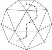
Figure 2. Example path in two dimensions for the last estimate in (67).

Any two elements in $\mathcal{T}_{h,T}$ are connected via a path over a bounded number of other elements in $\mathcal{T}_{h,T}$, and we can bound this last sum by one over facet terms (see Figure 2):

(67) $$\sum_{\tilde{T}\in\mathcal{T}_{h,T}}\sum_{S\in\mathcal{T}_{h,T}}h^{d}\Big{|}\big{(} \operatorname{curl}(E_{\tilde{T}}u)-\operatorname{curl}(E_{S}u)\big{)}\Big{|}\lesssim\sum_{F\in\mathcal{F}_{\omega}^{\circ}}h^{d}|\operatorname{curl}{(E_{T_{F,L}}u)}-\operatorname{curl}{(E_{T_{F,R}}u)}|^{2},$$

where $T_{F,L}$ and $T_{F,R}$ denote the two elements that share the facet $F$. Any facet is only summed up over a bounded number of times after reordering of the sum and due to the shape regularity of $\mathcal{T}_{h}$, (67) holds with a single constant for all patches in $\mathcal{T}_{h}$. These jump terms can be bounded an expansion of $E_{\tilde{T}}u$ at $x_{F}\mathrel{\mathop{\mathchar 58\relax}}=\Pi^{0}_{F}(x)$,

$$E_{\tilde{T}}u(x)=\Pi^{0}_{F}(E_{\tilde{T}}u)+\kappa(\operatorname{curl}{(E_{\tilde{T}}u)})\cdot(x-x_{F})\quad\text{for }x\in F,$$

and the elementary estimate $\|x-x_{F}\|_{F}^{2}\sim h^{2}|F|\sim h^{d+1}$. Writing $\mathcal{T}_{F}\mathrel{\mathop{\mathchar 58\relax}}=\{T_{F,L},T_{F,R}\}$, they show

$$h^{d}|\operatorname{curl}(E_{T_{F,L}}u)-\operatorname{curl}(E_{T_{F,R}}u)|^{2} \lesssim h^{-1}\|\kappa\big{(}\operatorname{curl}(E_{T_{F,L}}u)-\operatorname{curl}(E_{T_{F,R}}u)\big{)}\cdot(x-x_{F})\|_{F}^{2}$$

$$=h^{-1}\|(\Pi^{R}_{F}-\Pi^{0}_{F})\big{(}E_{T_{F,L}}u-E_{T_{F,R}}u\big{)}\|_{F}^{2}$$

$$\lesssim h^{-1}\|\Pi^{R}_{F}{[\![u]\!]}\|_{F}^{2}+\sum_{\tilde{T}\in\mathcal{T}_{F}}h^{-1}\|\Pi^{R}_{F}(u-E_{\tilde{T}}u)\|_{F}^{2}.$$

An $H^{1}$ trace inequality and (65) let us bound

$$h^{-1}\|\Pi^{R}_{F}(u-E_{\tilde{T}}u)\|_{F}^{2}\lesssim\|(u-E_{\tilde{T}}u)\|_{H^{1}(\tilde{T})}^{2}\lesssim\|{\varepsilon}(u)\|_{\tilde{T}}^{2},$$

in summary,

$$\sum_{\tilde{T}\in\mathcal{T}_{h,T}}\|\nabla(E_{\tilde{T}}u-R)\|_{\tilde{T}}^{2} \lesssim\sum_{F\in\mathcal{F}_{\omega}^{\circ}}h^{d}|\operatorname{curl}{(E_{T_{F,L}}u)}-\operatorname{curl}{(E_{T_{F,R}}u)}|^{2}\lesssim\sum_{\tilde{T}\in\mathcal{T}_{h,T}}\|{\varepsilon}(u)\|_{\tilde{T}}^{2}+\sum_{F\in\mathcal{F}_{\omega}^{\circ}}h^{-1}\|\Pi^{R}_{F}{[\![u]\!]}\|_{F}^{2},$$

i.e. (66) holds for our specific choice of $R$ which finishes the proof. ∎

Proof of Lemma 2.

An inverse estimate for the piecewise linear $\mathcal{I}_{\scriptscriptstyle f}u\in\bar{V}_{h}^{f}$ shows

$$\sum_{T\in\mathcal{T}_{h}}h^{-2}\|u-\mathcal{I}u\|_{T}^{2} \lesssim\sum_{T\in\mathcal{T}_{h}}h^{-2}\|u-\mathcal{I}_{\scriptscriptstyle f}u\|_{T}^{2}+h^{-2}\|(I-\pi_{0})\mathcal{I}_{\scriptscriptstyle f}u\|_{T}^{2}\lesssim\sum_{T\in\mathcal{T}_{h}}\Big{(}h^{-2}\|u-\mathcal{I}_{\scriptscriptstyle f}u\|_{T}^{2}+\sum_{F\in\mathcal{F}_{T}\cap\mathcal{F}_{h}^{\scriptscriptstyle D}}h^{-1}\|(I-\pi_{0})\mathcal{I}_{\scriptscriptstyle f}u\|_{F}^{2}\Big{)}.$$

As $(I-\pi_{0})\mathcal{I}_{\scriptscriptstyle f}u=\mathcal{I}_{\scriptscriptstyle f}u$ on $F\in\mathcal{F}_{h}^{\scriptscriptstyle D}$, and $\mathcal{I}_{\scriptscriptstyle f}u\in{\mathbb{P}}^{1}(\mathcal{T}_{h},\mathbb{R}^{{d}})$

$$\|(I-\pi_{0})\mathcal{I}_{\scriptscriptstyle f}u\|_{F}^{2}=\|\Pi^{1}_{F}\mathcal{I}_{\scriptscriptstyle f}u\|_{F}^{2} \lesssim\|\Pi^{R}_{F}\mathcal{I}_{\scriptscriptstyle f}u\|_{F}^{2}+\|(\Pi^{1}_{F}-\Pi^{R}_{F})\mathcal{I}_{\scriptscriptstyle f}u\|_{F}^{2}\lesssim\|\Pi^{R}_{F}u\|_{F}^{2}+\|\Pi^{R}_{F}(u-\mathcal{I}_{\scriptscriptstyle f}u)\|_{F}^{2}+\|(\Pi^{1}_{F}-\Pi^{R}_{F})\mathcal{I}_{\scriptscriptstyle f}u\|_{F}^{2}$$

We bound the second one with an $H^{1}$ trace inequality and a scaling argument,

$$h^{-1}\|\Pi^{R}_{F}(u-\mathcal{I}_{\scriptscriptstyle f}u)\|_{F}^{2}\lesssim h^{-2}\|u-\mathcal{I}_{\scriptscriptstyle f}u\|_{T}^{2}+\|\nabla(u-\mathcal{I}_{\scriptscriptstyle f}u)\|_{T}^{2},$$

where $T$ is the unique element such that $F\in\mathcal{F}_{T}$. An explicit expansion of the piecewise linear $\mathcal{I}_{\scriptscriptstyle f}u$ at the facet center of mass $x_{F}\mathrel{\mathop{\mathchar 58\relax}}=\Pi^{0}_{F}x$ shows

$$h^{-1}\|(\Pi^{1}_{F}-\Pi^{R}_{F})\mathcal{I}_{\scriptscriptstyle f}u\|_{F}^{2} =h^{-1}\|{\varepsilon}((\mathcal{I}_{\scriptscriptstyle f}u)_{|T})\cdot(x-x_{F})\|_{F}^{2}\lesssim\|{\varepsilon}(\mathcal{I}_{\scriptscriptstyle f}u)\|_{T}^{2}\lesssim\|{\varepsilon}(u)\|_{T}^{2}+\|\nabla(u-\mathcal{I}_{\scriptscriptstyle f}u)\|_{T}^{2}$$

Finally, with ${[\![\Pi_{F}^{R}u]\!]}=\Pi^{R}_{F}u$ on $F\in\mathcal{F}_{h}^{\scriptscriptstyle D}$, by Lemma 1 there holds

$$\sum_{T\in\mathcal{T}_{h}}h^{-2}\|u-\mathcal{I}u\|_{T}^{2} \lesssim\sum_{T\in\mathcal{T}_{h}}\Big{(}h^{-2}\|u-\mathcal{I}_{\scriptscriptstyle f}u\|_{T}^{2}+\|\nabla(u-\mathcal{I}_{\scriptscriptstyle f}u)\|_{T}^{2}+\|{\varepsilon}(u)\|_{T}^{2}+\sum_{F\in\mathcal{F}_{T}\cap\mathcal{F}_{h}^{\scriptscriptstyle D}}h^{-1}\|\Pi_{F}^{R}u\|_{F}^{2}\Big{)}$$

$$\lesssim\sum_{T\in\mathcal{T}_{h}}\Big{(}\|{\varepsilon}(u)\|_{T}^{2}+\sum_{F\in\mathcal{F}_{T}}h^{-1}\|\Pi_{F}^{R}{[\![u]\!]}\|_{F}^{2}\Big{)}.$$

The other volume terms $\|\nabla(u-\mathcal{I}u)\|_{T}$ in (17) are bounded analogously. ∎

Appendix B Trace estimates

The crucial step in the proof of (18) in [35] was to construct for a given $w\in{\mathbb{P}}^{{k}}(T,\mathbb{R})$ a $\tilde{w}\in{\mathbb{P}}^{{k}}(T,\mathbb{R})$ that approximates it in $\|\cdot\|_{j,F}$ and is bounded in the $H^{1}$ semi-norm and yet $\tilde{w}_{|\partial F}=0$. That is, implicitly, for $F\in\mathcal{F}_{h}$ and $T\in\mathcal{T}_{h}$ with $F\in\mathcal{F}_{T}$, an operator

(68) $$\begin{gathered}\mathcal{E}^{s,F}_{0}\mathrel{\mathop{\mathchar 58\relax}}{\mathbb{P}}^{{k}}(T,\mathbb{R})\rightarrow{\mathbb{P}}^{{k}}(T,\mathbb{R})\quad\textrm{with}\quad(\mathcal{E}_{0}^{s,F}u)_{|\partial F}=0\\ \textrm{and}\quad\|\nabla\mathcal{E}_{0}^{s,F}u\|_{T}^{2}+\|\mathcal{E}_{0}^{s,F}u-u\|^{2}_{j,F}\lesssim\log{{k}}\|u\|^{2}_{H^{1}(T)}\end{gathered}$$

was constructed. As no boundary conditions are enforced strongly in $\|\cdot\|_{1,F,0}$, the trace of $\mathcal{E}^{s,F}_{0}w$ could be extended to a function admissible for the infimum in $\|\cdot\|_{1,F,0}$. In addition to $\mathcal{E}^{s,F}_{0}$, of the commuting $H^{1},H(\operatorname{curl})$ and $H(\operatorname{div})$ extensions introduced in [19, 20, 21], we need the first,

$$\mathcal{E}^{s}\mathrel{\mathop{\mathchar 58\relax}}{\mathbb{P}}^{{k}}(\partial T,\mathbb{R})\rightarrow{\mathbb{P}}^{{k}}(T,\mathbb{R})$$

$$\textrm{with}\quad(\mathcal{E}^{s}u)_{\partial T}=u_{\partial T},\quad\textrm{and}\quad\|\mathcal{E}^{s}u\|_{H^{1}(T)}^{2}\lesssim\|u\|_{H^{1/2}(\partial T)}^{2},$$

see [19, Theorem 6.1], and last,

$$\mathcal{E}^{\operatorname{div}}\mathrel{\mathop{\mathchar 58\relax}}\{u\in H^{-1/2}(\partial T)\mathrel{\mathop{\mathchar 58\relax}}u_{|F}\in{\mathbb{P}}^{{k}}(F,\mathbb{R}^{d})~{}\forall F\in\mathcal{F}_{T}\}\rightarrow{\mathbb{P}}^{{k}}(T,\mathbb{R}^{d})$$

$$\textrm{with}\quad((\mathcal{E}^{\operatorname{div}}u)_{n})_{|F}=(u_{n})_{|F}~{}F\in\mathcal{F}_{T},\quad\textrm{and}\quad\|\mathcal{E}^{\operatorname{div}}u\|_{H^{1}(T)}^{2}\lesssim\|u\|_{H^{-1/2}(F)}^{2}.$$

Note although that $\mathcal{E}^{\operatorname{div}}$ was constructed from $H^{-1/2}(\partial T)\rightarrow H^{\operatorname{div}}(T)$ in [20, Theorem 7.1], the authors actually proved continuity in the $H^{1}(T)$ norm.

Lemma 10.

For $F\in\mathcal{F}_{h}$ and $u\in{\mathbb{P}}^{{k}}(T,\mathbb{R}^{{d}})$ there exists $\tilde{u}\in{\mathbb{P}}^{{k}}(T,\mathbb{R}^{{d}})$ with $\tilde{u}_{n}=u_{n}$ on $F$ and $\tilde{u}_{n}=0$ on $\tilde{F}\in\mathcal{F}_{T}\setminus\{F\}$ such that

(69) $$\|\nabla\tilde{u}\|_{T}^{2}+\|(\tilde{u}-u)_{t}\|_{j,F}^{2}+\sum_{\tilde{F}\in\mathcal{F}_{T}\setminus\{F\}}h^{-1}\|u_{t}\|_{j,\tilde{F}}^{2}\lesssim(\log{{k}})^{3}\|u\|_{H^{1}(T)}^{2}.$$

Proof.

To simplify the notation we only show a proof in three dimensions, the two-dimensional case works analogously. It also suffices to show the estimate on a reference tetrahedron, for general tetrahedra it follows from scaling arguments.

First, we use $\mathcal{E}^{\operatorname{div}}$ to get a $\tilde{u}_{1}$ which fulfills $(\tilde{u}_{1})_{n}=u_{n}$ on $F$ and $(\tilde{u}_{1})_{n}=0$ on $\tilde{F}\in\mathcal{F}_{T}\setminus\{F\}$ with bounded $H^{1}$ norm,

$$\|\tilde{u}_{1}\|_{H^{1}(T)}^{2}\lesssim\|u\|_{H^{-1/2}(F)}^{2}\lesssim\|u\|_{H(\operatorname{div},T)}^{2}\leq\|u\|_{H^{1}(T)}^{2}.$$

We have no control over the tangential traces of $\tilde{u}_{1}$ and have to add correction terms. For all $\hat{F}\in\mathcal{F}_{T}$ we pick two arbitrary normalized, orthogonal tangent vectors $t_{\hat{F}}$ and $\tilde{t}_{\hat{F}}$ and write the “errors” we need to compensate for on $F$ and $\tilde{F}\in\mathcal{F}_{T}\setminus\{F\}$ as

$$\lambda_{F}t_{F}\mathrel{\mathop{\mathchar 58\relax}}=\big{(}(u-\tilde{u}_{1})\cdot t_{F})t_{F}, \quad\quad\tilde{\lambda}_{F}\tilde{t}_{F}\mathrel{\mathop{\mathchar 58\relax}}=\big{(}(u-\tilde{u}_{1})\cdot\tilde{t}_{F}\big{)}\tilde{t}_{F},$$

$$\lambda_{\tilde{F}}t_{\tilde{F}}\mathrel{\mathop{\mathchar 58\relax}}=-\big{(}\tilde{u}_{1}\cdot t_{\tilde{F}}\big{)}t_{\tilde{F}}, \quad\quad\tilde{\lambda}_{\tilde{F}}\tilde{t}_{\tilde{F}}\mathrel{\mathop{\mathchar 58\relax}}=-\big{(}\tilde{u}_{1}\cdot\tilde{t}_{\tilde{F}}\big{)}\tilde{t}_{\tilde{F}}.$$

We write $\mathcal{E}^{s,\hat{F}}$ for $\mathcal{E}^{s}$ applied to the extension by zero to $\partial T$ of functions that vanish on $\partial\hat{F}$. This defines an $H_{00}^{1/2}$ stable extension

$$\mathcal{E}^{s,\hat{F}}\mathrel{\mathop{\mathchar 58\relax}}{\mathbb{P}}^{{k}}(F,\mathbb{R})\cap H_{00}^{1/2}(F)\rightarrow{\mathbb{P}}^{{k}}(T,\mathbb{R})\quad\textrm{with}\quad\|\mathcal{E}^{s,\hat{F}}u\|_{H^{1}(T)}\lesssim\|u\|_{H_{00}^{1/2}(F)}$$

and construct a corrected $\tilde{u}$ as

$$\tilde{u}~{}\mathrel{\mathop{\mathchar 58\relax}}=~{} \tilde{u}_{1}+\sum_{\hat{F}\in\mathcal{F}_{T}}\mathcal{E}^{s,\hat{F}}\mathcal{E}^{s,\hat{F}}_{0}(\lambda_{F})t_{\hat{F}}+\mathcal{E}^{s,\hat{F}}\mathcal{E}^{s,\hat{F}}_{0}(\tilde{\lambda}_{F})\tilde{t}_{\hat{F}},$$

where we understand $\mathcal{E}^{s,\hat{F}}$ to be applied to the respective trace on $\hat{F}$. The added corrections are normal bubbles because on their associated facet they are a scalar times a tangential and their trace vanishes on all others, i.e. $\tilde{u}_{n}=(\tilde{u}_{1})_{n}~{}\forall F\in\mathcal{F}_{T}$ and $\tilde{u}$ is admissible and we need to show that if fulfills (69).

As $\mathcal{E}^{s,\tilde{F}}$ restricted to $\tilde{F}$ is just the identity, for $\tilde{F}\in\mathcal{F}_{T}\setminus\{F\}$ there holds

$$\|\tilde{u}\cdot t_{\tilde{F}}\|_{j,\tilde{F}}^{2}=\|(\tilde{u}_{1}\cdot t_{\tilde{F}})-\mathcal{E}^{s,\tilde{F}}\mathcal{E}^{s,\tilde{F}}_{0}(\tilde{u}_{1}\cdot t_{\tilde{F}})\|_{j,\tilde{F}}^{2}=\|(I-\mathcal{E}^{s,\tilde{F}}_{0})(\tilde{u}_{1}\cdot t_{\tilde{F}})\|_{j,\tilde{F}}^{2}$$

and (68) implies

$$\|\tilde{u}\cdot t_{\tilde{F}}\|_{j,\tilde{F}}^{2}\lesssim\log{{k}}\|\tilde{u}_{1}\cdot t_{\tilde{F}}\|_{H^{1}(T)}^{2}\lesssim\log{{k}}\|\tilde{u}_{1}\|_{H^{1}(T)}^{2}\lesssim\log{{k}}\|u\|_{H^{1}(T)}^{2}.$$

The volume terms arising from the correction of $\lambda_{\tilde{F}}$ for $\tilde{F}\in\mathcal{F}_{T}\setminus\{F\}$ can be bounded with the inverse estimate $\|v\|_{H^{1/2}_{00}(\tilde{F})}\lesssim(\log{{k}})^{2}\|v\|_{H^{1/2}(\tilde{F})}$ for polynomials that vanish on $\partial\tilde{F}$, see [11, Lemma 4.7],

$$\|\nabla\mathcal{E}^{s,\tilde{F}}\mathcal{E}^{s,\tilde{F}}_{0}(\lambda_{\tilde{F}})t_{\tilde{F}}\|_{T}^{2}\lesssim\|\mathcal{E}^{s,\tilde{F}}_{0}\lambda_{\tilde{F}}\|_{H^{1/2}_{00}(\tilde{F})}^{2}\lesssim(\log{{k}})^{2}\|\mathcal{E}^{s,\tilde{F}}_{0}\lambda_{\tilde{F}}\|_{H^{1/2}(\tilde{F})}^{2},$$

and we can continue with (68) to see

$$\|\nabla\mathcal{E}^{s,\tilde{F}}\mathcal{E}^{s,\tilde{F}}_{0}(\lambda_{\tilde{F}})t_{\tilde{F}}\|_{T}^{2}\lesssim(\log{{k}})^{3}\|\tilde{u}_{1}\cdot t_{\tilde{F}}\|_{H^{1}(T)}^{2}\lesssim(\log{{k}})^{3}\|u\|_{H^{1}(T)}^{2}.$$

Analogously, we show these same bounds for volume and trace terms for $\tilde{F}=F$ as well as $\tilde{t}_{(\cdot)},\tilde{\lambda}_{(\cdot)}$ instead of $t_{(\cdot)},\lambda_{(\cdot)}$. In summary, we have

$$\|\nabla\tilde{u}\|_{T}^{2} +\|(u-\tilde{u})_{t}||_{j,F}^{2}+\sum_{\tilde{F}\in\mathcal{F}_{T}\setminus\{F\}}\|\tilde{u}_{t}\|_{j,\tilde{F}}^{2}$$

$$\lesssim~{} \|\nabla\tilde{u}_{1}\|_{F}^{2}+\sum_{\hat{F}\in\mathcal{F}_{T}}\|\nabla\mathcal{E}^{s,\hat{F}}\mathcal{E}^{s,\hat{F}}_{0}(\lambda_{\hat{F}})t_{\hat{F}}\|_{T}^{2}+\|\nabla\mathcal{E}^{s,\hat{F}}\mathcal{E}^{s,\hat{F}}_{0}(\tilde{\lambda}_{\hat{F}})\tilde{t}_{\hat{F}}\|_{T}^{2}+\|(u-\tilde{u})_{t}||_{j,F}^{2}+\sum_{\tilde{F}\in\mathcal{F}_{T}\setminus\{F\}}\|\tilde{u}_{t}\|_{j,\tilde{F}}^{2}$$

$$\lesssim~{} (\log{{k}})^{3}\|u\|_{H^{1}(T)}^{2}.$$

∎

Proof of Lemma 1.

For the minimizer $w$ in (19), a Korn inequality on $T$ shows

$$\|w\|_{H^{1}(T)}^{2} \lesssim\|{\varepsilon}(w)\|_{T}^{2}+\|\Pi^{R}_{F}w\|_{j,F}^{2}=\|{\varepsilon}(w)\|_{T}^{2}+\|\Pi^{R}_{F}(w-\hat{u})_{t}\|_{j,F}^{2}\lesssim\|(u,\hat{u})\|_{{\varepsilon},F}.$$

Choosing $\tilde{w}\in{\mathbb{P}}^{{k}}(T,\mathbb{R}^{d})$ as in Lemma 10, finishes the proof as it is admissible for the infimum in (20) and bounds it by $\|w\|_{H^{1}(T)}^{2}\lesssim\|(u,\hat{u})\|_{{\varepsilon},F}$. ∎

References

- [1] Netgen/ngsolve software.
- [2] Ngsamg software.
- [3] D. N. Arnold and F. Brezzi. Mixed and nonconforming finite element methods: implementation, postprocessing and error estimates. RAIRO Modél. Math. Anal. Numér., 19(1):7–32, 1985.
- [4] D.N. Arnold and F. Brezzi. Mixed and nonconforming finite element methods: implementation, postprocessing and error estimates. RAIRO Modél. Math. Anal. Numér., 19:7–32, 1985.
- [5] Douglas N Arnold, Franco Brezzi, Bernardo Cockburn, and L Donatella Marini. Unified analysis of discontinuous Galerkin methods for elliptic problems. SIAM journal on numerical analysis, 39(5):1749–1779, 2002.
- [6] Douglas N. Arnold, Richard S. Falk, and Ragnar Winther. Mixed finite element methods for linear elasticity with weakly imposed symmetry. Math. Comp., 76(260):1699–1723, 2007.
- [7] A. H. Baker, R. D. Falgout, T. V. Kolev, and U. M. Yang. Multigrid smoothers for ultraparallel computing. SIAM J. Sci. Comput., 33:2864–2887, 2011.
- [8] F. Bassi and S. Rebay. A high-order accurate discontinuous finite element method for the numerical solution of the compressible navier–stokes equations. Journal of Computational Physics, 131(2):267–279, March 1997.
- [9] Michele Benzi, Gene H. Golub, and Jörg Liesen. Numerical solution of saddle point problems. Acta Numerica, 14:1–137, 2005.
- [10] Sven Beuchler, Veronika Pillwein, and Sabine Zaglmayr. Sparsity optimized high order finite element functions for h(div) on simplices. Numerische Mathematik, 122(2):197–225, 2012.
- [11] Ion Bica. Iterative Substructuring Algorithms for the P-Version Finite Element Method for Elliptic Problems. Phd thesis, USA, 1997. AAI9808273.
- [12] Daniele Boffi, Franco Brezzi, and Michel Fortin. Mixed Finite Element Methods and Applications. Springer Science & Business Media, 2013.
- [13] Dietrich Braess. Finite Elemente - Theorie, schnelle Löser und Anwendungen in der Elastizitätstheorie. Springer, 2013.
- [14] Susanne C. Brenner. Korn’s inequalities for piecewise vector fields. Math. Comp., 73(247):1067–1087, 2004.
- [15] Franco Brezzi, Jim Douglas, Jr., Ricardo Durán, and Michel Fortin. Mixed finite elements for second order elliptic problems in three variables. Numer. Math., 51(2):237–250, 1987.
- [16] B. Cockburn, O. Dubois, J. Gopalakrishnan, and S. Tan. Multigrid for an HDG method†. IMA Journal of Numerical Analysis, 34(4):1386–1425, 10 2013.
- [17] Bernardo Cockburn, Jayadeep Gopalakrishnan, and Johnny Guzmán. A new elasticity element made for enforcing weak stress symmetry. Math. Comp., 79(271):1331–1349, 2010.
- [18] Bernardo Cockburn, Jayadeep Gopalakrishnan, and Raytcho Lazarov. Unified hybridization of discontinuous Galerkin, mixed, and continuous Galerkin methods for second order elliptic problems. SIAM Journal on Numerical Analysis, 47(2):1319–1365, 2009.
- [19] Leszek F. Demkowicz, Jay Gopalakrishnan, and Joachim Schöberl. Polynomial extension operators. part i. SIAM J. Numer. Anal., 46:3006–3031, 2008.
- [20] Leszek F. Demkowicz, Jay Gopalakrishnan, and Joachim Schöberl. Polynomial extension operators. part ii. SIAM J. Numer. Anal., 47:3293–3324, 2009.
- [21] Leszek F. Demkowicz, Jay Gopalakrishnan, and Joachim Schöberl. Polynomial extension operators. part iii. Math. Comput., 81:1289–1326, 2012.
- [22] B. Fraeijs de Veubeke. Displacement and equilibrium models in the finite element method by B. Fraeijs de Veubeke, Chapter 9, pages 145–197 of stress analysis, Edited by O. C. Zienkiewicz and G. S. Holister, Published by John Wiley & Sons, 1965. Internat. J. Numer. Methods Engrg., 52(3):287–342, 2001. Edited by O. C. Zienkiewicz and G. S. Holister and with introductory remarks by Zienkiewicz.
- [23] Guosheng Fu. Uniform auxiliary space preconditioning for HDG methods for elliptic operators with a parameter dependent low order term. SIAM Journal on Scientific Computing, 43(6):A3912–A3937, January 2021.
- [24] J. Gopalakrishnan, P. L. Lederer, and J. Schöberl. A mass conserving mixed stress formulation for the Stokes equations. IMA J. Numer. Anal., 40(3):1838–1874, 2019.
- [25] J. Gopalakrishnan, P. L. Lederer, and J. Schöberl. A mass conserving mixed stress formulation for Stokes flow with weakly imposed stress symmetry. SIAM J. Numer. Anal., 58(1):706–732, 2020.
- [26] Jay Gopalakrishnan, Lukas Kogler, Philip L. Lederer, and Joachim Schöberl. Minimal order h(div)-conforming velocity-vorticity approximations for incompressible fluids, 2021.
- [27] V. John, A. Linke, C. Merdon, M. Neilan, and L. Rebholz. On the divergence constraint in mixed finite element methods for incompressible flows. SIAM Review, 59:492–544, 2017.
- [28] Lukas Kogler and Joachim Schöberl. An algebraic multigrid method for elasticity based on an auxiliary topology with edge matrices. Numerical Linear Algebra with Applications, 29(1), August 2021.
- [29] P. Lederer and Joachim Schöberl. Polynomial robust stability analysis for H(div)-conforming finite elements for the Stokes equations. arXiv preprint arXiv:1612.01482, 2016.
- [30] P. L. Lederer. A Mass Conserving Mixed Stress Formulation for Incompressible Flows. Phd thesis, Technical University of Vienna, Wiedner Hauptstrasse 8-10, 1040 Vienna, Austria, 2019.
- [31] M. ”Schäfer, S. Turek, F. Durst, E. Krause, and R. Rannacher. Benchmark Computations of Laminar Flow Around a Cylinder, pages 547–566. Vieweg+Teubner Verlag, Wiesbaden, 1996.
- [32] J. Schöberl. NETGEN An advancing front 2D/3D-mesh generator based on abstract rules. Computing and Visualization in Science, 1(1):41–52, 1997.
- [33] J. Schöberl. C++11 implementation of finite elements in ngsolve, 2014.
- [34] Joachim Schöberl and Christoph Lehrenfeld. Domain Decomposition Preconditioning for High Order Hybrid Discontinuous Galerkin Methods on Tetrahedral Meshes, pages 27–56. Springer Berlin Heidelberg, Berlin, Heidelberg, 2013.
- [35] Joachim Schöberl and Christoph Lehrenfeld. Domain decomposition preconditioning for high order hybrid discontinuous galerkin methods on tetrahedral meshes. In Advanced Finite Element Methods and Applications, pages 27–56. Springer Berlin Heidelberg, 2013.
- [36] Benjamin Stamm and Thomas P. Wihler. -optimal discontinuous Galerkin methods for linear elliptic problems. Math. Comp., 79(272):2117–2133, 2010.
- [37] Rolf Stenberg. A family of mixed finite elements for the elasticity problem. Numerische Mathematik, 53(5):513–538, Aug 1988.
- [38] Andrea Toselli and Olof B Widlund. Domain decomposition methods. Springer series in computational mathematics. Springer, Berlin, Germany, 2005 edition, December 2005.
- [39] Rüdiger Verfürth. A combined conjugate gradient - multi-grid algorithm for the numerical solution of the stokes problem. Ima Journal of Numerical Analysis, 4:441–455, 1984.
- [40] Andrew J. Wathen and David J. Silvester. Fast iterative solution of stabilised stokes systems, part i: using simple diagonal preconditioners. SIAM Journal on Numerical Analysis, 30:630–649, 1993.
- [41] J. Xu. The auxiliary space method and optimal multigrid preconditioning techniques for unstructured grids. Computing, 56(3):215–235, September 1996.
- [42] Jinchao Xu. Iterative methods by space decomposition and subspace correction. SIAM Review, 34(4):581–613, December 1992.
- [43] Jinchao Xu and Ludmil Zikatanov. Algebraic multigrid methods. Acta Numerica, 26:591–721, 2017.
- [44] W. Zulehner. Analysis of iterative methods for saddle point problems: a unified approach. Math. Comput., 71:479–505, 2002.