Boosting Multivariate Structured Additive Distributional Regression Models

Abstract

We develop a model-based boosting approach for multivariate distributional regression within the framework of generalized additive models for location, scale, and shape. Our approach enables the simultaneous modeling of all distribution parameters of an arbitrary parametric distribution of a multivariate response conditional on explanatory variables, while being applicable to potentially high-dimensional data. Moreover, the boosting algorithm incorporates data-driven variable selection, taking various different types of effects into account. As a special merit of our approach, it allows for modelling the association between multiple continuous or discrete outcomes through the relevant covariates. After a detailed simulation study investigating estimation and prediction performance, we demonstrate the full flexibility of our approach in three diverse biomedical applications. The first is based on high-dimensional genomic cohort data from the UK Biobank, considering a bivariate binary response (chronic ischemic heart disease and high cholesterol). Here, we are able to identify genetic variants that are informative for the association between cholesterol and heart disease. The second application considers the demand for health care in Australia with the number of consultations and the number of prescribed medications as a bivariate count response. The third application analyses two dimensions of childhood undernutrition in Nigeria as a bivariate response and we find that the correlation between the two undernutrition scores is considerably different depending on the child’s age and the region the child lives in.

Keywords: GAMLSS; multivariate Gaussian distribution; multivariate logit model; multivariate Poisson distribution; model-based boosting; semiparametric regression.

1 Introduction

Many modern regression models relate certain characteristics of a univariate response distribution to explanatory variables. Examples include generalized additive models (GAMs; Hastie and Tibshirani,, 1990; Wood,, 2017) and quantile regression models (Koenker,, 2005), where with the former the conditional expectation and with the latter conditional quantiles of a univariate response distribution are modeled by an additive decomposition of different covariate effects. When multiple outcomes are supposed to be analyzed as response variables, one may fit such univariate regression models separately for each outcome. However, in practice, the components of a multivariate response are often not (conditionally) independent, so that separate models induce a loss of information and might lead to potentially misleading conclusions.

A well-known approach for the analysis of multivariate responses, particularly common in the economics literature, is called seemingly unrelated regression (Zellner,, 1962). This classical approach is restricted to linear predictors and constant covariance matrices not depending on the covariates; however, extensions to semiparametric predictors for the marginal means exist (Lang et al.,, 2003). Beyond that, multiple discrete responses (e.g., count data) can be analysed using seemingly unrelated Poisson regression (King,, 1989) and non-linear predictors (Gallant,, 1975). Similar to the approach of Zellner, (1962) these models are limited in their flexibility, and only the expected value of the response is linked to the covariates (Fiebig,, 2001). A more flexible framework is provided by generalized additive models for location, scale and shape (GAMLSS; Rigby and Stasinopoulos,, 2005), in which each parameter of the conditional distribution is modeled by an additive predictor. The use of additive predictors for all distribution parameters, such as location, scale or skewness parameters allows to incorporate different effect types for the covariates in a very flexible way.

In high-dimensional data situations in which the number of predictors exceeds the number of observations ($p>n$), several classical estimation approaches are no longer feasible. Bayesian variable selection (e.g., Zhu et al., 2012) and penalized regression methods (e.g., Wu et al., 2014; Liu and Sunil Rao, 2020) have been proposed for multivariate modelling in high-dimensional data situations. Nevertheless, GAMLSS based on penalized likelihood estimation is currently only available for univariate response variables. In contrast, Klein et al., (2015) extended this framework for multivariate responses to model the joint distribution of two or more responses in the spirit of GAMLSS relying on a fully Bayesian approach.

An alternative approach to penalized regression and Bayesian approaches is statistical boosting, which was originally developed in the field of machine learning and later extended to statistical modelling (Friedman et al.,, 2000; Friedman,, 2001). Its main features are the great flexibility regarding the effect types (e.g., spatial, smooth, or random effects) and the data-driven variable selection mechanism. The latter can be especially useful when the focus is on obtaining sparse models for a possibly high-dimensional covariate space (Bühlmann and Hothorn,, 2007). The concept of boosting has already been extended to distributional regression leading to an algorithm that is able to estimate and select additive predictors for all distribution parameters in univariate GAMLSS (Mayr et al., 2012a, ; Thomas et al.,, 2018).

In this work, we adapt the boosting algorithm for multivariate responses by combining the properties of GAMLSS and the main features of statistical boosting. Due to the structure of the algorithm, our approach is able to simultaneously model all distribution parameters and to select possible predictor effects in multivariate distributional regression models: The new multivariate boosting approach allows to model not only the marginals but also the association between multiple outcomes through an additive predictor.

Motivated by three biomedical applications, we focus on modeling and investigating specific bivariate regression models with emphasis on common parametric distributions in biomedical research: the bivariate Bernoulli distribution for binary outcomes, the bivariate Poisson distribution for count data and the bivariate Gaussian distribution for continuous outcomes (Marshall and Olkin,, 1985; Kocherlakota and Kocherlakota,, 1992; Kotz et al.,, 2000).

In the first biomedical application, the joint genetic predisposition for chronic ischemic heart disease and high cholesterol is analyzed based on a large cohort data from the UK Biobank (Sudlow et al.,, 2015) via the bivariate Bernoulli distribution. The main interest is to study the dependence of these phenotypes on the genetic variants and to discover possible joint associations of the two outcome variables, which is not feasible via classical approaches modeling the phenotypes separately (Burgess and Thompson,, 2015). In our case, we want to gain deeper insights into the relationship between the two phenotypes and the genetic variants affecting their association.

In the second application, we investigate effects for the demand on health care in Australia reported by Cameron and Trivedi, (1998) based on data from the Australian health survey. The two considered outcomes are the number of consultations with a doctor and the number of prescribed medications, whose association is modeled using the bivariate Poisson distribution for the covariates gender, age and annual income. The research question is based on a previous analysis by Karlis and Ntzoufras, (2005), however we illustrate that our approach offers higher flexibility.

In the last epidemiological application, two indicators for undernutrition, namely for acute and chronic undernutrition, of children in Nigeria are jointly analyzed, which is motivated by a previous analysis by Klein et al., (2015). The two scores are modeled with a bivariate Gaussian distribution, in which besides the marginal expectations also the scale parameter and the correlation parameter depend on covariates. In addition to several covariates describing the life situation of the children, the mother and the household they are living, spatial effects based on regional information are incorporated.

The structure of this article is as follows: Section 2 starts with a brief introduction to multivariate distributional regression models. Then we investigate the different bivariate regression models and give an insight into statistical boosting with a description of the extended algorithm. In Section 3 we illustrate different data settings using a simulation study while Section 4 illustrates the application on biomedical research questions for the considered distributional regression models in Section 2.

2 Boosting Multivariate Distributional Regression

2.1 The notion of multivariate distributional regression models

In multivariate structured additive distributional regression (Klein et al.,, 2015) it is assumed that the conditional distribution $\text{$\mathds{P}$}_{\text{\boldmath$Y$}|\text{\boldmath$X$}=\text{\boldmath$x$}}$ of a $D$-dimensional vector of responses $\text{\boldmath$Y$}=(Y_{1},\dots,Y_{D})^{\top}$ given covariate information summarized in $\text{\boldmath$X$}=\text{\boldmath$x$}$ has a $K$-parametric density $p(\text{\boldmath$y$}\mid\text{\boldmath$x$})=p(\text{\boldmath$y$}\mid{\text{\boldmath$\theta$}}(\text{\boldmath$x$}))$ with covariate dependent distribution parameters $\text{\boldmath$\theta$}(\text{\boldmath$x$})\equiv\text{\boldmath$\theta$}=(\theta_{1},\ldots,\theta_{K})^{\top}$.

Each distribution parameter $\theta_{k}$ is linked to a structured additive predictor $\eta_{k}$ (Fahrmeir et al.,, 2004) via bijective parameter-specific link functions $g_{k}$, such that $g_{k}(\theta_{k})=\eta_{k}$ and $g_{k}^{-1}(\eta_{k})=\theta_{k}$, $k=1,\ldots,K$. The inverse link functions $g_{k}^{-1}\equiv h_{k}$ are called response functions and ensure potential restrictions of the parameter space of $\theta_{k}$. The additive predictors $\eta_{k}$ depend on (possibly different) subsets of $x$ and are of the form

$$g_{k}(\theta_{k})=\eta_{k}=\beta_{0k}+\sum\limits_{j=1}^{p_{k}}f_{jk}(\text{\boldmath$x$}),\mbox{ for }k=1,\dots,K,$$

where $\beta_{0k}$ are the intercepts and each $f_{jk}$, $j=1,\ldots,p_{k}$, represents the functional effect of covariates $x$. The effects of the covariates can be specified in a very flexible manner and can correspond to linear, non-linear, random, interaction and further effects (see e.g., Fahrmeir et al.,, 2013; Wood,, 2017). Motivated by our applications in Section 4, in this work we focus on the following effect types:

1. Linear effects are represented by $f_{jk}(\text{\boldmath$x$})=\text{\boldmath$x$}_{jk}^{T}\text{\boldmath$\beta$}_{jk}$, where $\text{\boldmath$\beta$}_{jk}$ are the regression coefficients and $\text{\boldmath$x$}_{jk}$ is a covariate subset of $x$ for parameter $\theta_{k}$ ($\text{\boldmath$x$}_{jk}$ can be chosen individually for each parameter $\theta_{k}$).

2. Non-linear effects can be included using smooth functions $f_{jk}(\text{\boldmath$x$})$. As basis functions we use B-Splines with second order difference penalties (Eilers and Marx,, 1996).

3. Spatial effects based on observations assigned to discrete regions are incorporated using Markov random fields for modeling neighborhood structures $f_{jk}(\text{\boldmath$x$})=f_{jk}(s_{i})$, where $s_{i}$ denotes the region $s_{i}$ observation $i$ is located in (Rue and Held,, 2005).

2.2 Examples of relevant response distributions

In the following, we describe three common bivariate parametric distributions for binary, count and continuous responses, representing the most common response types in biomedical research. We will focus on the bivariate Bernoulli, the bivariate Poisson and the bivariate Gaussian distribution. While there are of course other multivariate distributions for discrete and continuous data (Johnson et al.,, 1997; Kotz et al.,, 2000), these three bivariate distributions are arguably most commonly used and are also relevant for our applications.

2.2.1 Bivariate Bernoulli distribution

For analyzing potentially correlated binary variables $\text{\boldmath$Y$}=(Y_{1},Y_{2})^{T}$, we consider the bivariate Bernoulli distribution with joint probability mass function

$$p(y_{1},y_{2})=p_{00}^{(1-y_{1})(1-y_{2})}p_{10}^{y_{1}(1-y_{2})}p_{01}^{(1-y_{1})y_{2}}p_{11}^{y_{1}y_{2}},~{}~{}y_{1},y_{2}\in\{0,1\},$$

where $p_{ij}=P(Y_{1}=i,Y_{2}=j)$, $i,j\in\{0,1\}$ are the joint probabilities. Then, the contingency table with marginal probabilities $p_{d}=\mathrm{P}(Y_{d}=1)$, $d=1,2$ is given by:

		$Y_{2}$
		0	1
$Y_{1}$	0	$p_{00}$	$p_{01}$	$1-p_{1}$
	1	$p_{10}$	$p_{11}$	$p_{1}$
		$1-p_{2}$	$p_{2}$	1

In a bivariate logistic regression model (logit model), the marginal probabilities $p_{1}=\mathrm{P}(Y_{1}=1)$ and $p_{2}=\mathrm{P}(Y_{2}=1)$, as well as the odds ratio $\psi=\frac{p_{00}p_{11}}{p_{01}p_{10}}$ describing the association between the two binary outcomes, can be estimated considering several covariates (McCullagh and Nelder,, 1989; Palmgren,, 1989). If $Y_{1}$ and $Y_{2}$ are independent, then the odds ratio $\psi=1$. The different additive predictors in the bivariate logit model are

$$\operatorname{logit}(p_{i}) =\eta_{p_{i}},\mbox{ for }i=1,2\quad\mbox{ and }\quad\log(\psi)=\eta_{\psi}.$$

The joint probability $p_{11}$ can be determined from the marginal probabilities $p_{1},p_{2}$ and the odds ratio $\psi$ via

$$p_{11}=\begin{cases}\frac{1}{2}(\psi-1)^{-1}\{a-\sqrt{a^{2}+b}\}&\,,\,\psi\neq 1\\ p_{1}p_{2}&\,,\,\psi=1,\end{cases}$$

where $a=1+(p_{1}+p_{2})(\psi-1)$ and $b=-4\psi(\psi-1)p_{1}p_{2}$ (Dale,, 1986). The joint probabilities $p_{10},p_{01}$ and $p_{00}$ can be derived from $p_{11}$ and the marginal probabilities.

An alternative approach for modeling bivariate binary responses is the bivariate probit model. However, in this work we focus on the logit model for two reasons: First, one distribution parameter directly corresponds to the odds ratio, which is easier to interpret and much more common in Biostatistics and biomedical research than the correlation of a latent bivariate response $\text{\boldmath$Y$}^{\ast}\sim N(\mathbf{0},\mathbf{\Sigma})$ for a probit model, where $Y_{d}=1\mbox{ if }Y_{d}^{\ast}>0\mbox{ and }0\mbox{ otherwise, }d=1,2$ and $\mathbf{\Sigma}$ a correlation matrix. Second, in a boosting and frequentist framework, the bivariate logit model is computationally favorable since it does not require the latent variables $\text{\boldmath$Y$}^{\ast}$.

2.2.2 Bivariate Poisson distribution

An important bivariate model for analyzing bivariate count data can be constructed from combining three random variables. If $Z_{k},k=1,2,3$ follow independent Poisson distributions with parameters $\lambda_{k}>0$, then the two random variables $Y_{1}=Z_{1}+Z_{3}$ and $Y_{2}=Z_{2}+Z_{3}$ follow a bivariate Poisson distribution with joint probability function given by

$$p(y_{1},y_{2})=\exp{(-(\lambda_{1}+\lambda_{2}+\lambda_{3}))}\frac{\lambda_{1}^{y_{1}}}{y_{1}!}\frac{\lambda_{2}^{y_{2}}}{y_{2}!}\sum\limits_{k=0}^{\min{(y_{1},y_{2})}}\binom{y_{1}}{k}\binom{y_{2}}{k}k!\left(\frac{\lambda_{3}}{\lambda_{1}\lambda_{2}}\right)^{k},~{}~{}y_{1},y_{2}\in\mathbb{N}_{0}.$$

The marginals also follow Poisson distributions with expectations $\mathbb{E}(Y_{1})=\lambda_{1}+\lambda_{3}$ and $\mathbb{E}(Y_{2})=\lambda_{2}+\lambda_{3}$. The parameter $\lambda_{3}$ controls the dependency between $Y_{1}$ and $Y_{2}$ and corresponds to the covariance $\mathrm{Cov}(Y_{1},Y_{2})=\lambda_{3}$. If the variables $Y_{1}$ and $Y_{2}$ are independent, then $\lambda_{3}=0$ and the bivariate Poisson distribution reduces to the product of two independent Poisson distributions. For further details on the bivariate Poisson distribution, see Kocherlakota and Kocherlakota, (1992) and Johnson et al., (1997).

In a bivariate Poisson model, each distribution parameter $\lambda_{k},\,k=1,2,3$ can be modeled in terms of several explanatory variables via

$$\log(\lambda_{k})=\eta_{\lambda_{k}},k=1,2,3,$$

where $\eta_{k}$ is the corresponding predictor for $\lambda_{k}$.

A drawback of this definition of the bivariate Poisson distribution is its property of modeling only data with positive correlations. An alternative was developed in Lakshminarayana et al., (1999) by defining the bivariate Poisson distribution as the product of Poisson marginals with a multiplicative factor. This definition also allows for negative correlations, but results in more difficult interpretations. A further alternative allowing for overdispersion in the marginal distributions is the bivariate negative binomial distribution (Kocherlakota and Kocherlakota,, 1992; Ma et al.,, 2020). We refrain from describing this distribution in more detail given our application in Section 4.2, where previous works have considered the bivariate Poisson distribution to be a reasonable modeling choice (Karlis and Ntzoufras,, 2005). In general, however, our approach of course would be also feasible for alternative parameterizations or alternative distributions.

2.2.3 Bivariate Gaussian distribution

The bivariate Gaussian distribution is one of the most commonly known distributions for considering two continuous responses. In this case, the random vector is written by $\text{\boldmath$Y$}\sim N(\text{\boldmath$\mu$},\mathbf{\Sigma})$, where the density of $\text{\boldmath$Y$}=(Y_{1},Y_{2})^{T}$ is given by

$$f(y_{1},y_{2})=\frac{1}{2\pi\sqrt{\mathrm{det}(\mathbf{\Sigma})}}\exp\left(-\frac{1}{2}(\text{\boldmath$y$}-\text{\boldmath$\mu$})^{T}\mathbf{\Sigma}^{-1}(\text{\boldmath$y$}-\text{\boldmath$\mu$})\right),~{}~{}y_{1},y_{2}\in\mathbb{R},$$

and $\text{\boldmath$\mu$}=(\mu_{1},\mu_{2})^{T}$ and $\mathbf{\Sigma}=\operatorname{Cov}(Y_{1},Y_{2})$ are its mean vector and covariance matrix, respectively. The latter is defined by

$$\mathbf{\Sigma}=\begin{pmatrix}\sigma_{1}^{1}&\rho\sigma_{1}\sigma_{2}\\ \rho\sigma_{1}\sigma_{2}&\sigma_{2}^{2}\end{pmatrix}$$

with marginal variances $\sigma^{2}_{1}=\operatorname{Var}(Y_{1})$ and $\sigma^{2}_{2}=\operatorname{Var}(Y_{2})$ and correlation parameter $\rho=\operatorname{Cor}(Y_{1},Y_{2})$. All parameters of the bivariate Gaussian distribution can be again modeled depending on covariates with parameter specific link-functions:

$$\mu_{1}=\eta_{\mu_{1}},\quad\mu_{2}=\eta_{\mu_{2}},\quad\log(\sigma_{1})=\eta_{\sigma_{1}},\quad\log(\sigma_{2})=\eta_{\sigma_{2}}\quad\mbox{and}\quad\rho/\sqrt{(1-\rho^{2})}=\eta_{\rho}.$$

For further practical and theoretical details of the bivariate Gaussian distribution, we refer to Kotz et al., (2000).

When the marginal distributions exhibit heavy tails, the bivariate $t$-distribution is an attractive alternative to the bivariate normal distribution. Motivated by our application on childhood undernutrition in Section 4.3, where the normality assumptions for the considered scores is reasonable (see e.g Klein et al.,, 2021), we omit details on the bivariate $t$-distribution in the context of structured additive distributional regression and refer to Klein et al., (2015) and references therein for further modeling details.

2.3 Estimation via model-based boosting

Boosting originally arose from the field of supervised machine learning (Freund,, 1995) but gained increasing popularity in statistics after the concept was adapted to fit statistical regression models (Friedman et al.,, 2000; Friedman,, 2001). Boosting algorithms are a flexible alternative to classical estimation approaches and have several practical advantages, such as the applicability to high-dimensional data problems and data-driven variable selection (Bühlmann and Hothorn,, 2007; Li et al.,, 2022; Wu and Ma,, 2019). In the context of regression, there exist different types of boosting algorithms (Tutz and Binder,, 2006; Bühlmann and Hothorn,, 2007). Here, we will focus on a component-wise gradient boosting algorithm with regression-type base-learners, which we refer to as statistical boosting (Mayr et al., 2014a, ; Mayr et al., 2014b, ).

This statistical boosting approach is based on minimizing a pre-specified loss function, which represents the regression problem and typically corresponds to the negative log-likelihood $l$ of the response distribution. In every iteration of the boosting algorithm, so-called base-learners are separately fitted to the negative gradient of the loss function, and the best-performing one is updated to the current estimate. A base-learner in our context is a regression function, and usually corresponds to one specific covariate effect in the additive predictor (e.g., a linear model as base-learner leads to a linear effect). An overview of possible base-learners can be found in Hofner et al., (2014).

For fitting multivariate distributional regression models, we extend the statistical boosting algorithm for generalized additive models for location, scale and shape (Mayr et al., 2012a, ) to multivariate distributions. A schematic overview of the selection of base-learners in one iteration of the boosting algorithm for multivariate responses can be found in Figure 1.

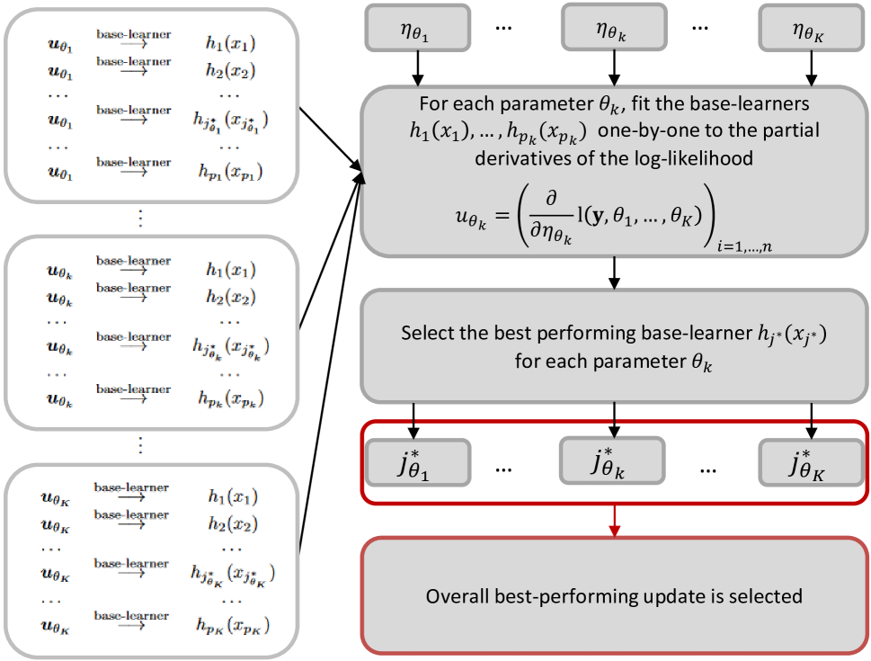
Figure 1: Graphical representation of boosting multivariate structured additive distributional regression (displaying one boosting iteration).

First, for each additive predictor $\eta_{k}$, $k=1,\dots,K$, a set of base-learners $h_{1}(x_{1}),\dots,h_{p_{k}}(x_{p_{k}})$ has to be specified in advance. Then, the partial derivative $u=\partial l/\partial\theta_{k}$ of the negative log-likelihood function $l$ with respect to the different distribution parameters $\theta_{k}$ is calculated and each base-learner is fitted separately to the gradient of the corresponding parameter $k$. For each parameter, the best performing base-learner $j_{k}^{*}$ is determined. After these best-fitting base-learners are selected for each dimension $k$, only the overall best update (with the highest loss reduction) of all distribution parameters is finally added to the corresponding additive predictor, with the estimated effect multiplied by a small fixed step-length, e.g., $\nu=0.1$. That means, in every iteration the best-fitting base-learner is determined for each distribution parameter and then compared across the different dimensions. This refers to a so-called non-cyclic version of boosting for distributional regression, leading to a single update of only one distribution parameter in each iteration (Thomas et al.,, 2018).

The main tuning parameter of the algorithm is the number of boosting iterations, which is typically chosen by cross-validation or resampling techniques. As the algorithm is usually stopped before convergence (early stopping), the optimization of the stopping iteration leads to the prevention of overfitting and encourages the sparsity of the resulting model by data-driven variable selection (Mayr et al., 2012b, ). In particular, those variables, whose corresponding base-learners have never been selected in the update process, are effectively excluded from the final model. The variable selection is simultaneously based on all additive predictors of the corresponding multivariate distribution. The algorithm does not impose any hierarchy between distribution parameters, but only judges the potential predictor variables based on their performance in increasing the joint likelihood. In addition, early stopping typically leads to an improvement in the prediction accuracy and shrinkage of the effect estimates. We provide an implementation of statistical boosting for multivariate distributional regression, which is integrated in the R package gamboostLSS (Hofner et al.,, 2016).

3 Simulations

To evaluate the performance of the proposed statistical boosting approach, we conducted a detailed simulation study for the three response distributions presented in Section 2.2. For each distribution, the particular settings are guided by the different applications in Section 4. With our simulations, we aim to answer the following questions:

• Does the boosting approach yield accurate estimates for the corresponding distribution parameters of the bivariate distributions?

• Can the boosting approach identify the truly informative variables and their effects?

• How do the bivariate models perform compared to univariate models that assume independence between the two response components?

In particular, we evaluate the estimation, variable selection and predictive performance. Note that for each considered simulation setting, different variables are informative for the distribution parameters and some of them partially overlap. Therefore, we refer to informative and non-informative variables and do not mention all of them individually for the different settings.

For all simulations, the step-length (learning rate) of the boosting algorithm is set to a fixed value of $\nu=0.1$ for each parameter of the bivariate models, as well as for the univariate boosted models. This is currently common practice in statistical boosting (Schmid and Hothorn,, 2008; Mayr et al., 2012a, ; Hofner et al.,, 2014). The stopping iteration $m_{\rm{stop}}$ is optimized by minimizing the empirical risk on an additional validation data set with $n_{\text{val}}=1500$ observations, following the same distribution as the training data. In addition, test data with 1000 observations were generated for the evaluation of the predictive performance (from the same distribution as the training data). A total of 100 simulation runs were performed for each simulation setting. The corresponding R code to reproduce the results is available on GitHub https://github.com/AnnikaStr/DistRegBoost.

3.1 Bivariate Bernoulli distribution

3.1.1 Simulation design

For the simulation of the bivariate logit model, we considered a high-dimensional setting with $n=1000$ observations and $p=1000$ covariates for each of the three parameters. For data generation, the R package VGAM (Yee,, 2021) was used, whereby the parameters $p_{1},p_{2}$ and $\psi$ were simulated with the following linear predictors

$$\operatorname{logit}(p_{1})=\eta_{\mu_{1}}=X_{1}+1.5X_{2}-X_{3}+1.5X_{4},\qquad \operatorname{logit}(p_{2})=\eta_{\mu_{2}}=2X_{1}-X_{2}+1.5X_{3},$$

$$\log(\psi)=\eta_{\psi}=-1.5+ 1X_{5}+1.5X_{6}.$$

Overall, only the first six covariates out of the $p=1000$ had a relevant effect on any of the distribution parameters (four for $p_{1}$, three for $p_{2}$ and two for $\psi$). The covariates were simulated from a multivariate normal distribution $N(\mathbf{0},\mathbf{\Sigma})$ with a Toeplitz covariance structure $\Sigma_{ij}=\rho^{|i-j|}$ for $1\leq i,j\leq p$, where $\rho=0.5$ is the correlation between consecutive variables $X_{j}$ and $X_{j+1}$. The covariates were incorporated in the boosting approach by using simple linear models as base-learners. As measures for the predictive performance, the area under the curve (AUC), the Brier score, the negative log-likelihood and energy score were considered. Note that the AUC and Brier score do not account for the dependence between the two outcomes and are calculated separately for both outcomes.

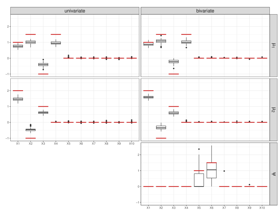
Figure 2: Results for the estimated linear effects of the univariate (left) and bivariate Bernoulli (right) model of the first ten covariates $X_{1},\dots,X_{10}$ from 100 simulation runs. The red horizontal lines correspond to the true values.

3.1.2 Results

Figure 2 presents the coefficient estimates of the first ten covariates $X_{1},\dots,X_{10}$ in form of boxplots resulting from 100 simulation runs for the univariate (left) and bivariate (right) model with the red horizontal lines corresponding to the true values. The univariate and bivariate models reflect the true structure for $\eta_{\mu_{1}}$ and $\eta_{\mu_{2}}$, as well as $\eta_{\psi}$ for the bivariate model, with both models leading to very similar results. The informative variables for $\mu_{1}$ and $\mu_{2}$ were almost selected in each simulation run, leading to an overall selection rate (average value over the informative variables) of 100% for the univariate models for both parameters and 100% for $\mu_{1}$ and 97.75% for $\mu_{2}$ in the bivariate model. The selection rate for $\psi$ is a bit lower than for the other parameters with a selection rate of 59% (see Appendix Table A3). The non-informative variables were selected very rarely overall, resulting in sparse models. A comparison of the predictive performance is provided in Table 1, showing that the univariate and bivariate models were very similar in terms of AUC, Brier score, and energy score, with the bivariate model having slightly better negative log-likelihood. In addition, the energy score for the univariate models showed a larger standard deviation. Further simulation results of this linear setting for a low-dimensional data situation ($p=10$ and $n=1000$) can be found in Appendix A.1.

	Univariate	Bivariate
AUC ($Y_{1}$)	0.88 (0.01)	0.88 (0.01)
AUC ($Y_{2}$)	0.85 (0.01)	0.84 (0.01)
Brier score ($Y_{1}$)	0.14 (0.01)	0.14 (0.01)
Brier score ($Y_{2}$)	0.16 (0.01)	0.16 (0.01)
Energy score	0.25 (0.19)	0.27 (0.01)
Negative log-likelihood	929.85 (22.46)	906.68 (27.32)

Table 1: Resulting predictive performance on independent test data for the linear setting of the bivariate Bernoulli distribution; mean (sd) values from 100 simulation runs are reported for the univariate and bivariate models.

3.2 Bivariate Poisson distribution

3.2.1 Simulation design

For the bivariate Poisson regression model, we investigated both linear and non-linear settings with $p=10$ covariates and $n=1000$ observations for each distribution parameter. For the linear setting, the underlying true predictors were specified as

$$\log(\lambda_{1})=\eta_{\lambda_{1}}=-X_{1}+0.5X_{2}+1.5X_{3}, \log(\lambda_{2})=\eta_{\lambda_{2}}=2X_{1}-X_{3}+1.5X_{4}+X_{5},$$ (1)

$$\log(\lambda_{3})=\eta_{\lambda_{3}}=0.5X_{5} +X_{6}-0.5X_{7},$$

where the covariates followed a multivariate normal distribution $N(\mathbf{0},\mathbf{\Sigma})$ with Toeplitz covariance structure and correlation coefficient $\rho=0.5$. Thus, the first seven covariates were informative for any of the distribution parameter (three for $\lambda_{1}$ and $\lambda_{3}$, four for $\lambda_{2}$). For this setting, simple linear models were incorporated as base-learners. For the non-linear setting, the true additive predictors were given by

$$\log(\lambda_{1})=\eta_{\lambda_{1}}=\sqrt{X_{1}}X_{1}, \log(\lambda_{2})=\eta_{\lambda_{2}}=\cos(2X_{2}),$$ (2)

$$\log(\lambda_{3})=\eta_{\lambda_{3}} =\sin{X_{3}},$$

where the covariates were independently simulated from the uniform distribution $U(0,1)$ and only one covariate was informative for each of the distribution parameters. As base-learners, we chose P-splines (20 equidistant knots with a second-order difference penalty and four degrees of freedom). The R extraDistr package from Wolodzko, (2020) was used to simulate data from the bivariate Poisson regression model.

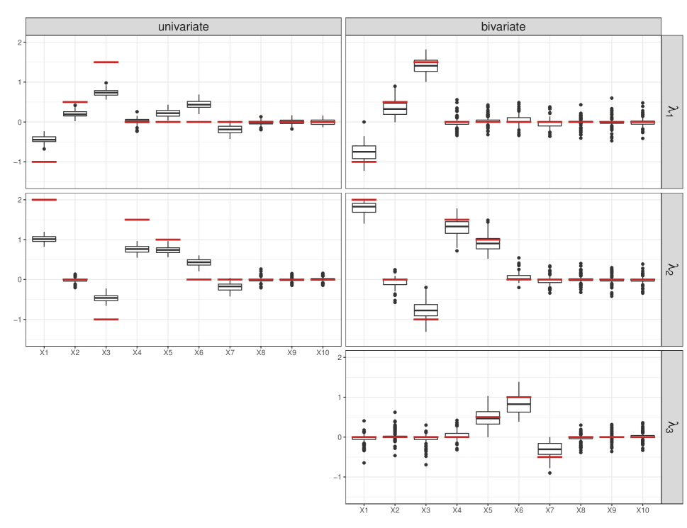
Figure 3: Results for the estimated linear effects of the univariate (left) and bivariate Poisson model (right) from 100 simulation runs. The horizontal lines correspond to the true values.

3.2.2 Results

Figure 3 displays the coefficient estimates for the linear Poisson regression models (A.2.2). The boxplots present the estimated coefficients of the 100 simulation runs for the univariate (left) and bivariate models (right). Overall, boosting the bivariate regression model was able to identify the informative variables and to accurately estimate the true effects represented by the red horizontal lines. In comparison, the univariate models for $\lambda_{1}$ and $\lambda_{2}$ resulted in much smaller estimated coefficients. For both models, the informative variables were selected in almost every simulation run: considering $\lambda_{1}$ and $\lambda_{2}$, the univariate models and the bivariate model had a selection rate of almost 100% for the informative variables, whereby also for $\lambda_{3}$ a high selection rate of 95.67% for the informative variables was achieved. On the other hand, the univariate models as well as the bivariate model selected also several non-informative variables with a small coefficient size. A more detailed overview on the selection rates for the specific parameters can be found in Table A4 of the Appendix.

Furthermore, we considered the MSEP, the negative log-likelihood, and the energy score for the evaluation of the predictive performance on test data (see Table A10). The MSEP only accounts for the marginal distributions and displays here a slightly better performance for the univariate models. The negative log-likelihood and the energy score, which also take the association into account, showed a better performance for the bivariate model.

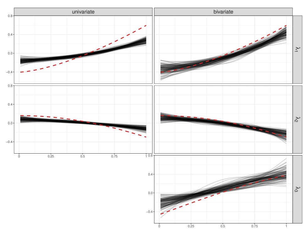
Figure 4: Results for the estimated non-linear effects for the univariate (left) and the bivariate Poisson model (right) from 100 simulation runs. The red dotted lines correspond to the true effects.

Figure 4 displays the effect estimates for the non-linear setting (2). Overall, the estimated splines approximate the true effects well for each parameter of the bivariate model and clearly outperform the univariate models for $\lambda_{1}$ and $\lambda_{2}$. The informative variables were selected in each simulation run. However, as in the linear model, we observed also high selection rates for the non-informative variables in both models (see Appendix A.2).

In terms of predictive performance, similar to the linear setting, the MSEP indicated a better performance of the univariate models, while the bivariate models outperformed the univariate models in terms of the negative log-likelihood as expected. The energy score is very similar for both models but slightly better for the bivariate model overall. Further simulation results for these settings in case of high-dimensional data with $p=1000$ covariates and $n=1000$ observations can be found in Appendix A.2.

	Linear model		Non-linear model
	Univariate	Bivariate	Univariate	Bivariate
MSEP ($Y_{1}$)	2.66 (0.18)	3.96 (0.29)	4.64 (0.25)	8.18 (0.65)
MSEP ($Y_{2}$)	2.86 (0.23)	4.11 (0.34)	5.49 (0.29)	9.06 (0.68)
Energy score	1.48 (1.11)	1.36 (0.03)	1.95 (0.04)	1.95 (0.04)
Negative log-likelihood	3598.42 (54.31)	3413.68 (40.91)	4433.06 (52.06)	4246.96 (42.58)

Table 2: Resulting predictive performance on independent test data for the linear and non-linear settings of the bivariate Poisson regression; mean (sd) values from 100 simulation runs are reported for the univariate and bivariate models.

3.3 Bivariate Gaussian distribution

3.3.1 Simulation design

For the simulation of a bivariate Gaussian distributed outcome, we considered a setting with linear, non-linear and spatial effects with $p=10$ covariates and $n=1000$ observations with the following true predictors

$$\mu_{1}=\eta_{\mu_{1}}=\sin(2X_{1})/0.5+X_{6}+0.5X_{7}+f_{\text{spat}}\qquad \mu_{2}=\eta_{\mu_{2}}=2+3\cos(2X_{2})+0.5X_{7}+X_{8}+f_{\text{spat}}$$

$$\log(\sigma_{1})=\eta_{\sigma_{1}}=\sqrt{X_{3}}X_{3}-0.5X_{8}+f_{\text{spat}}\qquad \log(\sigma_{2})=\eta_{\sigma_{2}}=\cos(X_{4})X_{4}+0.25X_{9}+f_{\text{spat}}$$

$$\rho/\sqrt{1-\rho^{2}}=\eta_{\rho}=\log(X_{5}^{2}) +X_{10}+f_{\text{spat}},$$

where the covariates were independently simulated from the uniform distribution $U(0,1)$. Each included covariate was informative for one of the distribution parameters; more precisely, for each parameter three covariates, one linear and one non-linear, and additionally the spatial effect. For linear effects we used simple linear models as base-learners and P-splines for the non-linear effects. The spatial effects were simulated with $f_{\text{spat}}(s)=\sin(x^{c}_{s})\cos(0.5y^{c}_{s}),s\in{1,\dots,S}$, based on the centroids of the standardized coordinates of the discrete regions in Western Germany with overall $S=327$ regions. The neighborhood structure was modeled by the spatial base-learner using a Markov random field (based on the R package BayesX by Umlauf et al.,, 2019).

	Univariate	Bivariate
MSEP ($Y_{1}$)	1.59 (0.11)	1.59 (0.11)
MSEP ($Y_{2}$)	1.38 (0.07)	1.38 (0.07)
Energy score	1.03 (0.02)	1.01 (0.02)
Negative log-likelihood	3370.41 (89.59)	3098.11 (109.97)

Table 3: Resulting predictive performance on independent test data of the bivariate Gaussian regression; mean (sd) values from 100 simulation runs are reported for the univariate and bivariate models.

3.3.2 Results

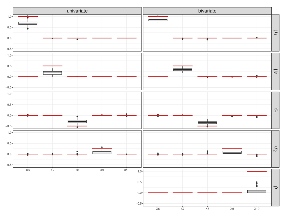
Figure A4: Results for the estimated linear effects of the univariate (left) and bivariate Gaussian regression model (right) for the low-dimensional setting from 100 simulation runs. The horizontal lines correspond to the true values.

Considering the linear effects (see Figure A4 in Appendix A.3), the effect estimates from the 100 simulation runs for both models reflect the true structures of the linear part of the predictors, whereby the bivariate model better approximates the true values. The bivariate model was also able to capture the true non-linear functions well (Figure 5); only small deviations are observed for the variance and for the correlation $\rho$ at the left border. The results for the univariate models appear to be very similar regarding the univariate effects and can be found in the Appendix (Figure A5). For the spatial effects, the true structure for the regions in West Germany was identified by each distribution parameter (a graphical representation of the true structure and the estimated spatial effects are in Appendix A.3).

The informative variables for the univariate and bivariate models were selected in nearly all 100 simulation runs, where the bivariate model also correctly selected the informative variables for the correlation between the outcomes. Whereas, we can not examine the correlation with the univariate models. The selection rates for the non-informative variables were slightly higher for the bivariate model (see Appendix Table A7).

Regarding predictive performance, the MSEP, the energy score, and the negative log-likelihood were considered. For the MSEP and the energy score, similar results were observed for the univariate and the bivariate models. The negative log-likelihood on the test set showed an improvement in predictive performance considering the bivariate model. Further simulation results for this setting in case of high-dimensional data with $p=1000$ covariates and $n=1000$ observations can be found in Appendix A.3.

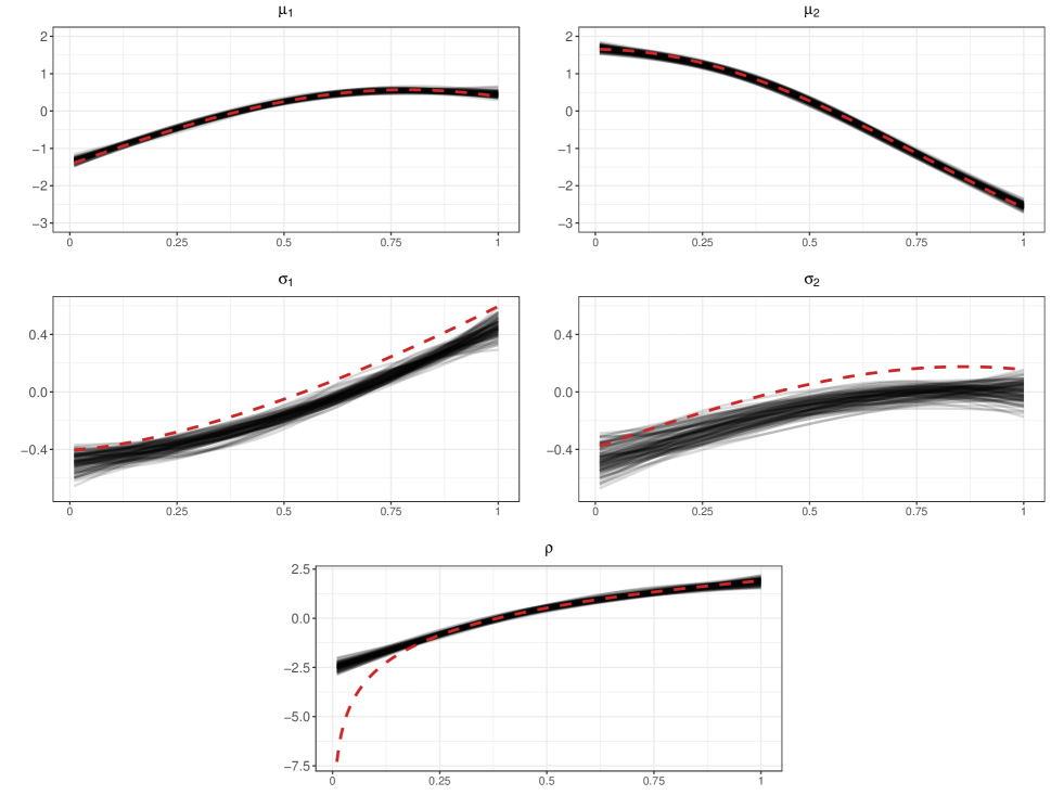
Figure 5: Results for the estimated non-linear effects of the bivariate Gaussian regression model from 100 simulation runs. The red dotted lines correspond to the true effects.

3.4 Summary

Overall, we obtained promising results for all three considered distributional regression families (logistic, Poisson and Gaussian regression), highlighting that the boosting algorithm yields appropriate estimates for the different parameters and is capable of identifying the most informative variables from a potentially much larger set of candidate variables. The comparison with the univariate models showed that the estimated effects for the bivariate model was able to provide better approximations to the true structure of the predictors than the univariate models (particularly for the Poisson and Gaussian regression models). We noticed that for the logistic regression model, the selection rates for the association parameter, the odds ratio, tended to be lower than for the association parameter of the bivariate Poisson and Gaussian distribution. Furthermore, the number of selected non-informative variables was higher for the univariate as well as the bivariate models for the Poisson distribution. However, the linear low-dimensional setting for the bivariate logistic regression model (see Appendix A.1) and the low-dimensional Gaussian regression model showed higher selection rates in this situation as well (Appendix A.3). Conclusively, this highlights a tendency of the algorithm to select more non-informative variables in low-dimensional settings.

Regarding prediction accuracy, as expected, the univariate and bivariate models performed similarly for evaluation criteria that consider only the marginals (AUC, brier score and MSEP). Only for the Poisson distribution, the univariate model performed slightly better regarding the MSEP. This can be explained by the particular design of this bivariate distribution, i.e. the summation of the means for both outcomes ($\mathbb{E}(Y_{1})=\lambda_{1}+\lambda_{3}$ and $\mathbb{E}(Y_{2})=\lambda_{2}+\lambda_{3}$). In Figure 3, for example, we observe that the informative variables $X_{5},X_{6}$ and $X_{7}$ for parameter $\lambda_{3}$ were selected quite frequently with a higher estimated coefficient in the univariate models. These wrongly selected variables for the marginals resulted in an improvement of the MSEP. In the bivariate model, we account for the association between $Y_{1}$ and $Y_{2}$ by modeling the dependency in terms of the covariates. The MSEP does not account for the association and the variables describing dependency are not reflected in the marginals as in the univariate models.

Regarding the predictive scores which account for associations between the outcomes, the energy score tended to be very similar for the univariate and bivariate models, while the negative log-likelihood was consistently better for the bivariate models.

4 Biomedical applications

In this section we consider three diverse biomedical data sets to illustrate the applicability of our extended boosting approach for multivariate distributional regression models based on binary, count and continuous outcomes presented in Section 2.2.

4.1 Genetic predisposition for chronic ischemic heart disease and high cholesterol

For analyzing the association between high cholesterol and chronic ischemic heart disease in dependency of different genetic variants, we used cohort data from the UK Biobank. The UK Biobank is a large biomedical cohort study containing genetic and health information from over half a million British participants (Sudlow et al.,, 2015).

In classical approaches for analyzing a potential genetic liability to a specific phenotype such as high cholesterol or chronic heart disease, each considered genetic variant is fitted individually to the phenotype using a simple linear model (Burgess and Thompson,, 2015). In this context, previous works including genome-wide association studies (e.g., Linsel-Nitschke et al.,, 2008; Richardson et al.,, 2020) have investigated to find genetic variants associated with high cholesterol and heart disease. Using our boosting algorithm for multivariate distributional regression, the main interest here is to investigate the association between chronic ischemic heart disease and high cholesterol, both considered as binary phenotypes (high cholesterol $>$ 6.16 mmol/l). In particular, we aim to identify genetic variants affecting their association by estimating the two phenotypes jointly in a bivariate logistic model. That means we do not only want to model the individual distributions of the two phenotypes, but also estimate the dependency between these phenotypes as a function of genetic variants, which is not possible with conventional approaches.

The considered data set consists of 20,000 randomly sampled observations of individuals with white British ancestry, with additional 10,000 observations used to validate the optimal stopping iteration. For each phenotype, 1000 variants were selected in a pre-screening step based on the largest marginal associations between the variants and the phenotype, which were computed with the PLINK2 function -variant-score (Purcell and Chang, 2015; Chang et al., 2015). After pre-screening, the data set contains a total of 1865 variants (with 135 variants selected for both phenotypes). Variants with minor allele frequency not less than 1% were randomly sampled with the-thin-count function. Missing genotypes were imputed by the reference allele using the R package bigsnpr (Privé et al.,, 2018).

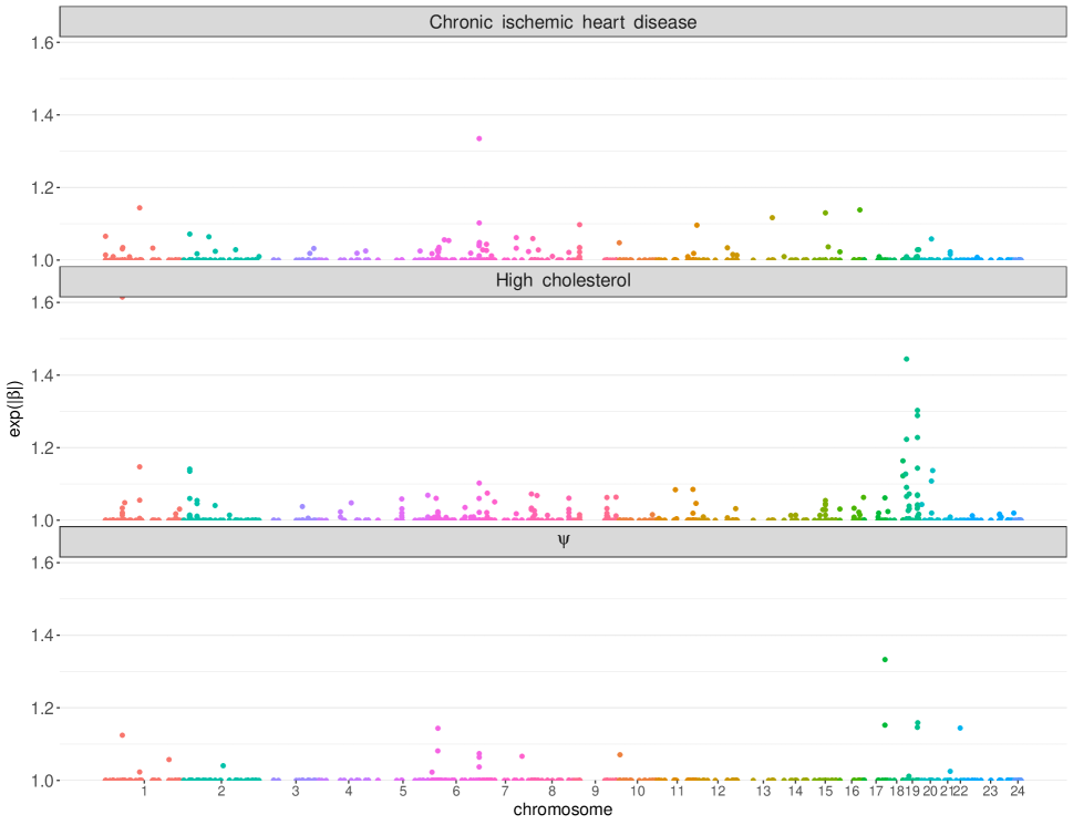
Figure 6: Manhattan plots for the coefficient estimates (expressed in exponential absolute values of the estimated coefficients) of the boosted bivariate logistic regression model of the joint analysis of high cholesterol and ischemic heart disease from the UK Biobank data. The $x$-axis represents the genomic location of the variants.

Figure 6 shows the resulting estimated coefficients (expressed in exponential absolute values of the estimated coefficients) for the three distribution parameters. When comparing these Manhattan plots with the classical univariate ones (based on the marginal association evaluated on the $-\log 10(P)$ scale) for high cholesterol and chronic ischemic heart disease, we find that the bivariate boosting model tended to identify variants with a higher coefficient value (stronger effect) from similar or the same genomic locations, where the univariate models also showed large univariate associations (see Appendix B.1).

For high cholesterol, e.g., the variants with the smallest univariate p-values are located on chromosomes 18 and 19; on these chromosomes there were also the variants that had the highest estimated coefficients in the bivariate boosting model. These findings are consistent with the location of known cholesterol-associated genes (Richardson et al.,, 2020). Variants from these chromosomes were also selected with our approach for the odds ratio. Our model selected several variants for chronic ischemic heart disease that are in line with the findings of the meta-analysis of genome-wide association studies examining DNA sequence variants associated with ischemic heart disease of Elosua and Sayols-Baixeras, (2017) (e.g., the variants rs11206510, rs2891168 and rs4420638).

Overall, several variants were selected by the boosting approach for each distributional regression parameter, i.e., 75 for $\mu_{1}$, 154 for $\mu_{2}$, and 19 variants for $\psi$. For each parameter, mainly those variants were selected that were primarily filtered due to the specific phenotype (the 1000 most highly associated from the univariate screening). In particular, for $\mu_{1}$, 63 of the 75 selected variants had been primarily chosen for ischemic heart disease, so that 12 of the 75 selected variants for $\mu_{1}$ also had a large univariate association with high cholesterol. Regarding high cholesterol, 110 variants were selected from the ones that had been pre-selected, while 44 of the selected variants for high cholesterol had been originally pre-selected for ischemic heart disease. The two marginal means $\mu_{1}$ and $\mu_{2}$ had six selected variants in common, and both had one variant that was also selected for the odds ratio $\psi$ (namely for $\mu_{1}$: rs10455872 and for $\mu_{2}$: rs77542162). The odds ratio included two variants that were among the 1000 most highly correlated pre-selected variants for both phenotypes, namely rs505151 and rs2229094. The other 17 variants selected for the odds ratio were divided as follows: 10 from $\mu_{1}$ (ischemic heart disease) and 7 from $\mu_{2}$ (high cholesterol). This means the algorithm identified several variants that affect the dependency between the two phenotypes. The odds ratio is the most common measure for examining the dependency between two binary outcomes in biomedical research and the interpretation in our context is very similar. Thus, the selected variants for the association parameter have an effect on both outcomes, with a positive effect increasing the association between heart disease and high cholesterol and conversely.

In summary, our algorithm provides the ability to study the joint genetic predisposition for chronic ischemic heart disease and high cholesterol. With our approach we can also model the dependence of the association between these two phenotypes on genetic variants, which is not possible with classical approaches. In addition, in line with the literature on cardiovascular genetics, our model selected several variants in genomic regions which had been previously identified to be relevant for the considered phenotypes.

4.2 Demand for health care in Australia

The first analysis on the demand for health care in Australia, based on the Australian health survey from 1977 to 1978, was reported by Cameron and Trivedi, (1998). The considered data set consists of $n=5,190$ observations (which is only a subset of the overall collected survey). The bivariate count variables of interest are the number of consultations with a doctor (in the past 2 weeks) and the number of prescribed medications (used in the last two days), which we model using bivariate Poisson regression. The explanatory variables are gender (female coded as 1, male as 0), age (in years divided by 100) and annual income (in Australian dollars; AUD; divided by 1000, measured as midpoints of coded ranges). More details on the survey and its original analysis can be found in Cameron and Trivedi, (1998). The data are provided in the R package bivpois (Karlis and Ntzoufras,, 2005), which is available on GitHub (https://github.com/cran/bivpois).

In the following, we use the same representation of the bivariate Poisson distribution as introduced in Section 2.2.2. Each distribution parameter $\lambda_{k},k=1,2,3$ is modelled based on explanatory variables. We consider the two following models:

1. Gender, age and income are included as covariates for $\lambda_{\text{consulations}}$ (number of doctor consultations) and $\lambda_{\text{medications}}$ (number of medications prescribed), but only gender is considered as a covariate for the covariance parameter $\lambda_{3}$ (corresponding to Mod. (b) in Karlis and Ntzoufras, (2005)).

2. For each model parameter, P-splines are used as base-learners for the continuous variables age and income, while for gender linear effects are used.

	Covariate	$\lambda_{\text{consulations}}$	$\lambda_{\text{medications}}$	$\lambda_{3}$
Mod. A	Intercept	-2.10	-2.20	-2.62
	Gender (female)	0.05	0.59	0.61
	Age	1.40	3.29	-
	Income	-0.31	-0.10	-
Mod. B	Intercept	-2.29	-2.22	-0.35
	Gender (female)	0.13	0.60	0.19

Table 4: Results of the bivariate Poisson model for the demand of Health Care for Mod. A and Mod. B (see Figure 7 for the non-linear effect estimates for age and income in Mod. B).

Considering the results of Mod. A presented in the upper part of Table 4, we observe that with increasing age, both the numbers of doctor consultations and prescribed medications are estimated to increase. Income has negative marginal effects on both responses, which means that higher income is associated with fewer prescribed medications and fewer doctor appointments. For the covariance parameter $\lambda_{3}$, only gender was included as an explanatory variable in Mod. A. The joint effect of gender on the number of doctor consultations and prescribed medications indicates that males and females have different covariance terms. The estimated effect of 0.61 for gender suggests that the association between numbers of consultations and medications is higher for women than for men.

The lower part of Table 4 and Figure 7 present the results for Mod. B. With an increasing age up to 50 years, the number of doctor consultations is estimated to increase linearly, with a slight decrease starting around the age of 57 years. The estimated effect of age on the number of prescribed medications and the covariance parameter is linear and is negative throughout the covariance. The income is estimated to have a U-shape effect for the medical consultation, with a minimum between 800 AUD and 1,150 AUD. The estimated effect of gender for Mod. A is slightly larger than for Mod. B.

Overall, the estimated effects of Mod. A are consistent with the results of Karlis and Ntzoufras, (2005). In addition, we also considered a non-linear model. Both the linear and non-linear models indicated that the expected numbers of doctor consultations and prescribed medications increase with age. For income, the expected numbers of doctor visits and prescribed medications decreases with increasing income for Mod. A. The expected number of doctor visits also decreases in Mod. B as income increased, whereby a U-shaped effect for income can be observed.

Furthermore, because of the bivariate modeling, we also obtain information about the relationship between the outcomes. Here, both models showed a higher association between the number of doctor consultations and prescribed medications for women. Furthermore, Mod. B also included age and income as covariates for the covariance parameter and the model suggested that the association becomes greater with increasing age.

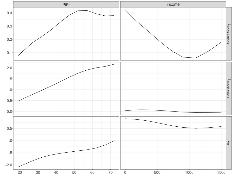
Figure 7: Partial effects of age and income on the demand for health care in Australia for Mod. B.

4.3 Risk factors for undernutrition in Nigeria

To analyze childhood undernutrition, a large database is available from the Demographic and Health Survey (DHS, https://dhsprogram.com/), containing nationally representative information about the population’s health and nutrition status in numerous developing and transition countries. Here, we consider a data set used in Klein et al., (2021) which contains data from Nigeria collected in 2013 with overall $23,042$ observations (after exclusion of outliers and inconsistent observations). The bivariate responses are stunting, which is defined as stunted growth measured as the insufficient height of the child concerning its age (chronic undernutrition), and wasting, which refers to insufficient weight for height (acute undernutrition). We analyze the joint distribution of these two responses using the bivariate Gaussian distribution with covariate-dependent marginal means and standard deviations as well as a covariate-dependent correlation parameter.

For continuous variables, P-splines were applied as base-learners, namely for cage (age of the child in months), edupartner (years of partner’s education), mage (age of the mother in years) as well as mbmi (body mass index of the mother). Several other categorical covariates (12 covariates in total, e.g., bicycle, car, cbirthorder) were included using simple linear models as base-learners. Furthermore, the neighborhood structure of the districts in Nigeria was incorporated and modeled by the spatial base-learner using a Markov random field. For a full description of the explanatory variables, see Appendix B.2.

Figure 8 and 9 show the results for the non-linear and spatial effects for all parameters. The estimated linear effects are given in Appendix Table B2. Stunting is estimated to be more affected by variables describing children’s living situation, particularly ctwin (child is a twin) and the birth order (cbirthorder). Following our model, with higher birth order, the stunting score decreases, with negative values indicating that the children’s growth is below the expected growth of a child with normal nutrition. For wasting, ctwin had the largest effect, displaying also an increased risk for acute undernutrition. These results are in line with those of Klein et al., (2021).

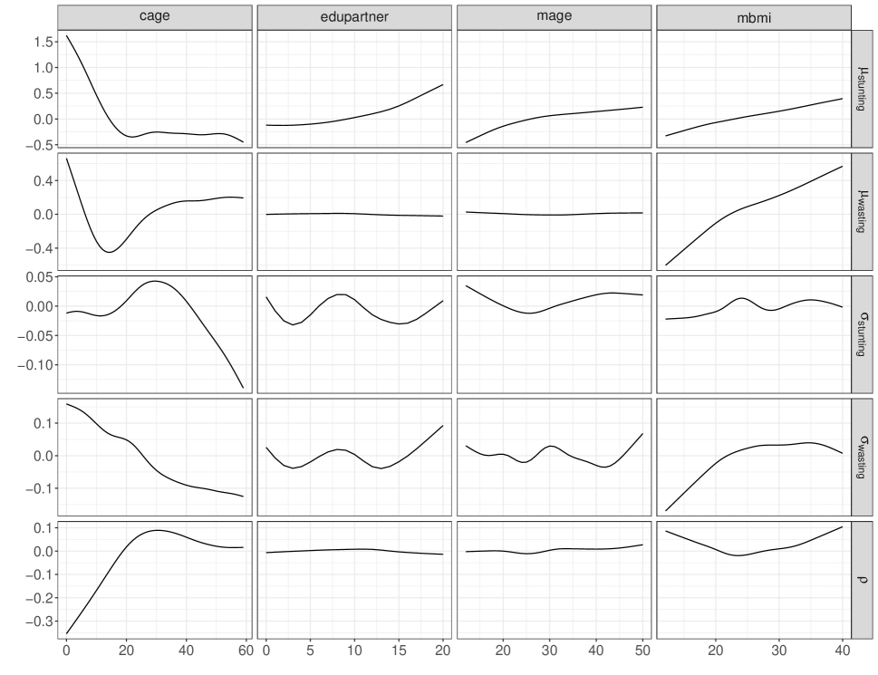
Figure 8: Non-linear effects of cage, edupartner, mage and mbmi for stunting and wasting of the bivariate Gaussian regression model for the Nigeria data.

Furthermore, stunting and wasting were both influenced by cage and mbmi as well. Following our model, for mbmi, a higher BMI of the mother indicates a higher acute and chronic undernutrition. For cage, stunting and wasting is estimated to decrease (i.e. risk increases) up to around 20 months. After 20 months, the risk for wasting is estimated to decrease again while remaining similar for stunting.

The scale parameter for wasting, for example, indicates a higher variability for the age of children up to around 25 months. For children older than 25 months, the variability decreases slightly, whereby we observed a greater variability for stunting between 20 and 40 months. The correlation is negative for children younger than 20 months and is approximately zero after a small positive correlation between 20 and 50 months. This finding indicates an interaction between stunting and wasting depending on the child’s age, which is non-linear and stronger for younger children. Thus, children with a greater height in the first years of life have a lower weight for height and vice versa. The other covariates have only a minor estimated effect on the correlation parameter. These results are consistent with previous findings (Klein et al.,, 2015, 2021), which also holds for the spatial effects. The regional effect was selected to be informative for all distribution parameters. The effect of chronic undernutrition, for example, showed a lower risk of stunted growth in regions in southern Nigeria due to a positive effect. These regions also have a lower variability of chronic undernutrition compared to the average regions in the center of the county. This means that in this part of Nigeria the score for stunting is estimated to be on average lower and its variability is also smaller. By contrast, the regions in the north are estimated to have a higher risk for stunting. In terms of the correlation, some regions in the north are estimated to have a negative effect, while other regions in the south are estimated to show a slight positive effect on the correlation. A positive effect suggests that these regions have a problem of acute undernutrition as well as chronic undernutrition.

Figure 9: Spatial structure of stunting and wasting in Nigeria for the distribution parameters of the Gaussian distribution.

Overall, chronic undernutrition (stunting) is mostly affected by the living conditions of the children, for example, the birth order. Whereby, stunting and wasting were both influenced by the mother’s BMI and particularly by the child’s age. Additional effects of the covariates on the scale and correlation parameters also suggested greater uncertainty for younger children for acute undernutrition through a positive effect on the standard deviation, with variability decreasing with age. Furthermore, we observed a stronger negative correlation between stunting and wasting in younger children, i.e., as stunting increases, wasting is expected to be lower. This means that children with a greater height tend to suffer from a lower weight for height at a younger age.

5 Discussion

We developed statistical boosting for modeling distributional regression with multivariate outcomes. Motivated by our biomedical applications, we considered three important multivariate parametric distributions: the bivariate Bernoulli, Poisson and Gaussian distributions. As special merits over classical maximum likelihood or Bayesian approaches to multivariate GAMLSS, our boosting framework can directly be used for high-dimensional data problems ($p\gg n$), while allowing for a data-driven variable selection mechanism that allows for sparse models for all parameters of a multivariate distribution.

In simulation studies, we have illustrated that the proposed boosting approach is able to identify the correct predictors in different data situations, including low- and high-dimensional settings and incorporating different effect types such as spatial effects. A comparison with the boosted univariate models showed that the bivariate models yielded more accurate estimates for the true structure of the effects.

The wide applicability of our approach is illustrated on three different biomedical data sets, where we extend previous studies and also confirm findings from the literature. Applying our approach to examine jointly the genetic predisposition for chronic ischemic heart disease and high cholesterol not only provides information on the dependency of these phenotypes on the genetic variants, but also allows to identify the variants that affect the association between both phenotypes. This is in strong contrast to classical methods to estimate e.g., polygenic risk scores via accumulating effects from univariate linear models with single variants as predictor variables (Choi et al.,, 2020). Our approach does not only incorporate multivariable predictor models, but also considers multivariate outcomes and hence allows to assess also the genetic predisposition for the association between several phenotypes, such as heart disease and high cholesterol. To the best of our knowledge, this is the first time multivariate distributional regression was adapted to model the joint genetic liability for multiple phenotypes.

In examining possible effects of patients characteristics on demand for health care, we found that age and income are relevant predictors, but also that gender affected the association between the number of doctor consultations and prescribed medications, with a stronger association found for women (cf. Karlis and Ntzoufras,, 2005).

In the third application analyzing the risk of undernutrition in Nigeria, an association was found between chronic undernutrition and the child’s living condition. In addition, the age of the child had a relevant influence on all distribution parameters related to chronic and acute undernutrition; furthermore, the regional effect was selected not only for the margins but also for the scale and correlation parameters.

A limitation regarding the considered distributions in our approach is the restriction of the Poisson distribution to positive dependency between the two responses. A possible solution for this restriction in future research could be the use of alternative parametrizations (Lakshminarayana et al.,, 1999), which also allow for modeling negative correlations; however, these have the disadvantage that the interpretation of effects on these parameters becomes much more difficult. A limitation of our algorithm is the relatively high selection rates for variables with only minor importance, which occurs particularly in low-dimensional settings. In this context, Strömer et al., (2022) have recently proposed an approach to deselect predictors with negligible impact to obtain sparser models with statistical boosting. We want to investigate the incorporation of this proposal in the context of multivariate GAMLSS in the future. Moreover, as the number of distribution parameters and the complexity of the model increases (e.g., due to many non-linear effects), the algorithm becomes computationally more intensive. To address this problem, also alternative approaches for early stopping could be considered. A promising approach in the future which has been developed for univariate location models is probing, where randomly shuffled versions of the original observed variables (probes) are added to the data set and the algorithm stopped when the first probe is selected (Thomas et al.,, 2017).

Last, our focus has been on bivariate distributional regression models, but we will consider extending the models to higher dimensional responses in future research. From an algorithmic perspective, the extension should be straight-forward as it only adds more distributional parameters in our proposed framework. However, not only the construction of appropriate response distributions but also the interpretation of the effect estimates becomes more challenging. For example, for the multivariate Gaussian distribution, the main challenge is the parameterization of the covariance matrix and a promising route here could be based on a (modified) Cholesky decomposition (Pourahmadi,, 2011). Similar, the extension of the bivariate Poisson distribution to higher dimensions has some difficulties due to the complicated form of the joint probability function. The most common extension would force all the pairs of variables to have the same covariance (Karlis,, 2003), whereby Karlis and Meligkotsidou, (2005) already discussed a model with a two-way covariance term that allows for different covariances between the variables.

Supplementary Materials

A supplement contains further information on the simulation and biomedical applications.

Acknowledgement

The work on this article was supported by the Deutsche Forschungsgemeinschaft (DFG, grant number 428239776, KL3037/2-1, MA7304/1-1).

Supplementary Materials

Appendix A Further simulation results

A.1 Bivariate Bernoulli distribution

A.1.1 Low-dimensional setting

For the simulation of a low-dimensional setting of the bivariate logit model, we considered $n=1000$ observations and $p=10$ covariates for each of the three parameters. For data generation, the R package VGAM (Yee,, 2021) was used, whereby the parameters $p_{1},p_{2}$ and $\psi$ were simulated with the following linear predictors

$$\operatorname{logit}(p_{1}) =\eta_{\mu_{1}}=X_{1}+1.5X_{2}-X_{3}+1.5X_{4},$$

$$\operatorname{logit}(p_{2}) =\eta_{\mu_{2}}=2X_{1}-X_{2}+1.5X_{3},$$

$$\log(\psi) =\eta_{\psi}=-1.5+1X_{5}+1.5X_{6}.$$

Overall, only the first six covariates out of the $p=10$ had a relevant effect on any of the distribution parameters (four for $p_{1}$, three for $p_{2}$ and two for $\psi$). The covariates were simulated from a multivariate normal distribution $N(\mathbf{0},\mathbf{\Sigma})$ with a Toeplitz covariance structure $\Sigma_{ij}=\rho^{|i-j|}$ for $1\leq i,j\leq p$, where $\rho=0.5$ is the correlation between consecutive variables $X_{j}$ and $X_{j+1}$. The covariates were incorporated in the boosting approach by using simple linear models as base-learners. As measures for the predictive performance, the area under the curve (AUC), the Brier score, the negative log-likelihood and energy score were considered. Note that the AUC and Brier score do not account for the dependence between the two outcomes and are calculated separately for both outcomes.

Parameter	Univariate		Bivariate
	inf	non-inf	inf	non-inf
$\mu_{1}$	100%	86.83%	99.75%	32.17%
$\mu_{2}$	100%	92.57%	100%	42.14%
$\psi$	-	-	75.50%	19.88%

Table A5: Resulting selection rates of the low-dimensional setting of the bivariate Bernoulli distribution; the average values from the 100 simulation runs are reported for the univariate and bivariate model for the informative and non-informative variables.

	Univariate	Bivariate
AUC ($Y_{1}$)	0.89 (0.01)	0.88 (0.01)
AUC ($Y_{2}$)	0.86 (0.01)	0.86 (0.01)
Brier score ($Y_{1}$)	0.14 (0.01)	0.14 (0.01)
Brier score ($Y_{2}$)	0.15 (0.01)	0.15 (0.01)
Energy score	0.22 (0.23)	0.27 (0.01)
Negative log-likelihood	882.03 (24.05)	874.97 (26.80)

Table A6: Resulting predictive performance on independent test data for the low-dimensional linear setting of the bivariate Bernoulli distribution; mean (sd) values from 100 simulation runs are reported for the univariate and bivariate models.

Figure A1: Results for the estimated linear effects of the univariate (left) and bivariate Bernoulli (right) model of the ten covariates $X_{1},\dots,X_{10}$ for the low-dimensional setting from 100 simulation runs. The red horizontal lines correspond to the true values.

A.1.2 High-dimensional setting

Parameter	Univariate		Bivariate
	inf	non-inf	inf	non-inf
$\mu_{1}$	100%	5.18%	97.75%	1.26%
$\mu_{2}$	100%	5.93%	100%	1.57%
$\psi$	-	-	59%	0.17%

Table A7: Resulting selection rates of the high-dimensional setting of the bivariate Bernoulli distribution; the average values from the 100 simulation runs are reported for the univariate and bivariate model for the informative and non-informative variables.

A.2 Bivariate Poisson distribution

A.2.1 Low-dimensional setting

	Linear model				Non-linear model
Parameter	Univariate		Bivariate		Bnivariate		Bivariate
	inf	non-inf	inf	non-inf	inf	non-inf	inf	non-inf
$\lambda_{1}$	98.67%	75.29%	98.67%	54.43%	100%	46.56%	100%	77.56%
$\lambda_{2}$	100%	73.17%	100%	57.67%	100%	45.22%	100%	84.11%
$\lambda_{3}$	-	-	95.67%	49.43%	-	-	100%	53.78%

Table A8: Resulting selection rates of the low-dimensional linear and non-linear setting of the bivariate Poisson regression; the average values from the 100 simulation runs are reported for the univariate and bivariate model for the informative and non-informative variables.

A.2.2 High-dimensional setting

We investigated in the linear and non-linear settings with $p=1000$ covariates and $n=1000$ observations for each distribution parameter. For the linear setting, the underlying true predictors were specified as

$$\log(\lambda_{1}) =\eta_{\lambda_{1}}=-X_{1}+0.5X_{2}+1.5X_{3},$$

$$\log(\lambda_{2}) =\eta_{\lambda_{2}}=2X_{1}-X_{3}+1.5X_{4}+X_{5},$$

$$\log(\lambda_{3}) =\eta_{\lambda_{3}}=0.5X_{5}+X_{6}-0.5X_{7},$$

where the covariates followed a multivariate normal distribution $N(\mathbf{0},\mathbf{\Sigma})$ with Toeplitz covariance structure and correlation coefficient $\rho=0.5$. Thus, the first seven covariates were informative for any of the distribution parameter (three for $\lambda_{1}$ and $\lambda_{3}$, four for $\lambda_{2}$). For this setting, simple linear models were incorporated as base-learners. For the non-linear setting, the true additive predictors were given by

$$\log(\lambda_{1}) =\eta_{\lambda_{1}}=\sqrt{X_{1}}X_{1},$$

$$\log(\lambda_{2}) =\eta_{\lambda_{2}}=\cos(2X_{2}),$$

$$\log(\lambda_{3}) =\eta_{\lambda_{3}}=\sin{X_{3}},$$

where the covariates were independently simulated from the uniform distribution $U(0,1)$ and only one covariate was informative for each of the distribution parameters. As base-learners, we chose P-splines (20 equidistant knots with a second-order difference penalty and four degrees of freedom).

Parameter	Linear model				Non-linear model
	Univariate		Bivariate		Univariate		Bivariate
	inf	non-inf	inf	non-inf	inf	non-inf	inf	non-inf
$\lambda_{1}$	70.67%	0.83%	70.33%	1.48%	100%	0.54%	100%	0.90%
$\lambda_{2}$	96.00%	1.03%	96.00%	1.93%	97%	0.41%	100%	2.26%
$\lambda_{3}$	-	-	62.33%	0.79%	-	-	75.00%	0.01%

Table A9: Resulting selection rates of the high-dimensional linear and non-linear setting of the bivariate Poisson regression; the average values from the 100 simulation runs are reported for the univariate and bivariate model for the informative and non-informative variables.

Figure A2: Results for the estimated linear effects of the univariate (left) and bivariate Poisson model (right) of the first ten covariates $X_{1},\dots,X_{10}$ for the high-dimensional setting from 100 simulation runs. The horizontal lines correspond to the true values.

Figure A3: Results for the estimated non-linear effects of the univariate (left) and the bivariate Poisson model (right) of the first ten covariates $X_{1},\dots,X_{10}$ for the high-dimensional setting from 100 simulation runs. The red dotted lines correspond to the true effects.

	Linear model		Non-linear model
	Univariate	Bivariate	Univariate	Bivariate
MSEP ($Y_{1}$)	2.65 (0.16)	3.94 (0.25)	4.58 (0.26)	7.12 (0.39)
MSEP ($Y_{2}$)	3.06 (0.26)	4.24 (0.34)	5.47 (0.35)	8.03 (0.51)
Energy score	1.40 (0.04)	1.40 (0.03)	1.94 (0.05)	1.94 (0.05)
Negative log-likelihood	3630.27 (49.83)	3454.63 (39.48)	4422.52 (58.82)	4250.49 (47.49)

Table A10: Resulting predictive performance on independent test data for the linear and non-linear settings of the bivariate Poisson regression for the high-dimensional setting; mean (sd) values from 100 simulation runs are reported for the univariate and bivariate models.

A.3 Bivariate Gaussian distribution

A.3.1 Low-dimensional setting

Figure A5: Results for the estimated non-linear effects of the univariate Gaussian regression models for the low-dimensional setting from 100 simulation runs. The red dotted lines correspond to the true effects.

Parameter	Univariate		Bivariate
	inf	non-inf	inf	non-inf
$\mu_{1}$	100%	50.00%	100%	57.29%
$\mu_{2}$	100%	48.14%	100%	50.86%
$\sigma_{1}$	100%	59.29%	100%	61.57%
$\sigma_{2}$	100%	57.43%	100%	65.14%
$\rho$	-	-	98.5%	20.57%

Table A11: Resulting selection rates of the low-dimensional linear and non-linear setting of the bivariate Gaussian regression; the average values from the 100 simulation runs are reported for the univariate and bivariate model for the informative and non-informative variables.

Figure A6: Map of the true structure of the spatial effect of West Germany.

Figure A7: The estimated spatial effects for one simulation run of the low-dimensional setting of the bivariate Gaussian regression model.

A.4 High-dimensional setting

For the simulation of a low-dimensional setting of a bivariate Gaussian distributed outcome, we considered a setting with linear, non-linear and spatial effects with $p=1000$ covariates and $n=1000$ observations with the following true predictors

$$\mu_{1}=\eta_{\mu_{1}}=\sin(2X_{1})/0.5+X_{6}+0.5X_{7}+f_{\text{spat}}\qquad \mu_{2}=\eta_{\mu_{2}}=2+3\cos(2X_{2})+0.5X_{7}+X_{8}+f_{\text{spat}}$$

$$\log(\sigma_{1})=\eta_{\sigma_{1}}=\sqrt{X_{3}}X_{3}-0.5X_{8}+f_{\text{spat}}\qquad \log(\sigma_{2})=\eta_{\sigma_{2}}=\cos(X_{4})X_{4}+0.25X_{9}+f_{\text{spat}}$$

$$\rho/\sqrt{1-\rho^{2}}=\eta_{\rho}=\log(X_{5}^{2}) +X_{10}+f_{\text{spat}},$$

where the covariates were independently simulated from the uniform distribution $U(0,1)$. Each included covariate was informative for one of the distribution parameters; more precisely, for each parameter three covariates, one linear and one non-linear, and additionally the spatial effect. For linear effects we used simple linear models as base-learners and P-splines for the non-linear effects. The spatial effects were simulated with $f_{\text{spat}}(s)=\sin(x^{c}_{s})\cos(0.5y^{c}_{s}),s\in{1,\dots,S}$, based on the centroids of the standardized coordinates of the discrete regions in Western Germany with overall $S=327$ regions. The neighborhood structure was modeled by the spatial base-learner using a Markov random field (Umlauf et al.,, 2019).

	Univariate	Bivariate
MSEP ($Y_{1}$)	1.59 (0.10)	1.58 (0.10)
MSEP ($Y_{2}$)	1.38 (0.09)	1.38 (0.09)
Energy score	1.03 (0.02)	1.00 (0.02)
Negative log-likelihood	3339.99 (97.13)	2997.21 (94.28)

Table A12: Resulting predictive performance on independent test data for the high-dimensional setting of the bivariate Gaussian regression; mean (sd) values from 100 simulation runs are reported for the univariate and bivariate models.

Parameter	univariate		bivariate
	inf	non-inf	inf	non-inf
$\mu_{1}$	100%	0.68%	100%	1.07%
$\mu_{2}$	100%	0.59%	100%	0.82%
$\sigma_{1}$	100%	1.58%	100%	1.31%
$\sigma_{2}$	100%	1.77%	100%	1.35%
$\rho$	-	-	94.5%	0.09%

Table A13: Resulting selection rates of the high-dimensional linear and non-linear setting of the bivariate Gaussian regression; the average values from the 100 simulation runs are reported for the univariate and bivariate model for the informative and non-informative variables.

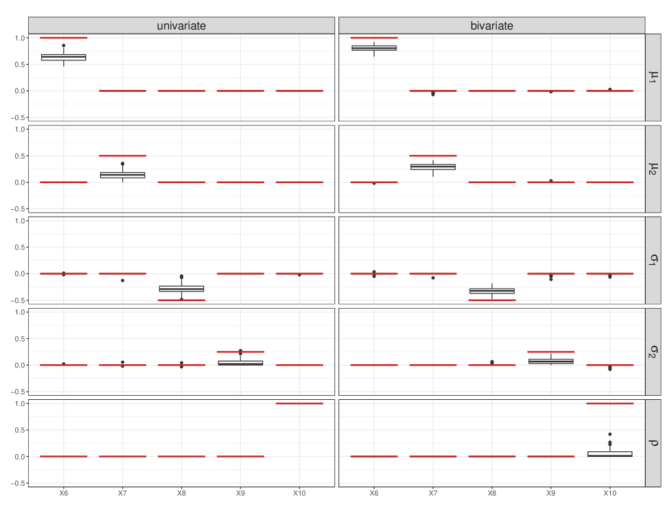
Figure A8: Results for the estimated linear effects of the univariate (left) and bivariate Gaussian regression model (right) for the high-dimensional setting from 100 simulation runs. The horizontal lines correspond to the true values.

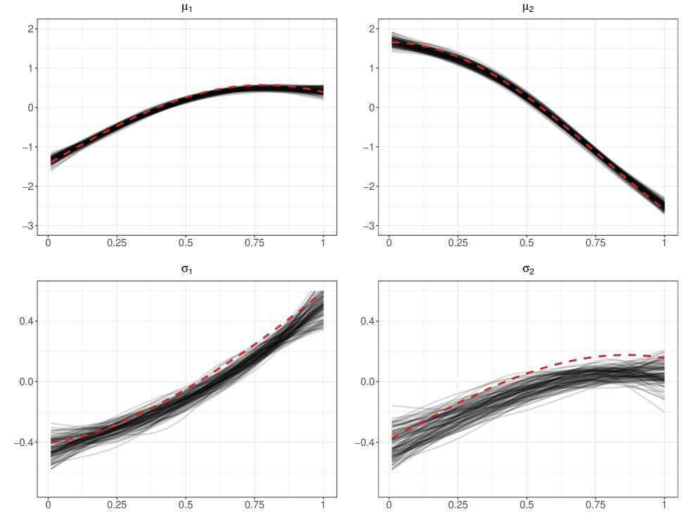
Figure A9: Results for the estimated non-linear effects of the univariate Gaussian regression model for the high-dimensional setting for 100 simulation runs. The red dotted lines correspond to the true effects.

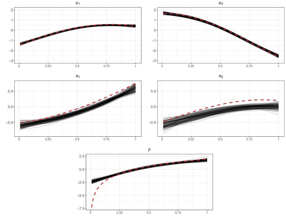
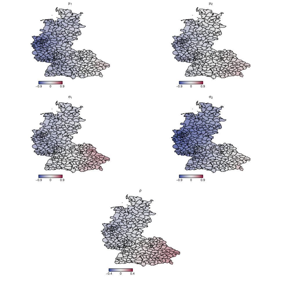
Figure A10: Results for the estimated non-linear effects of the bivariate Gaussian regression model for the high-dimensional setting for 100 simulation runs. The red dotted lines correspond to the true effects.

Figure A11: The estimated spatial effects for one simulation run of the high-dimensional setting of the bivariate Gaussian regression model.

Appendix B Biomedical applications

B.1 Genetic predisposition for chronic ischemic heart disease and high cholesterol

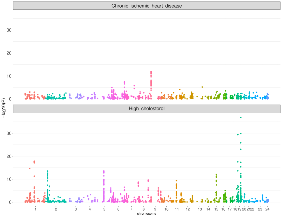
Figure A12: Manhattan plot for the marginal association of the genetic variants on high cholesterol and chronic ischemic heart disease on the $-\log 10(P)$ scale.

B.2 Risk factors for undernutrition in Nigeria

Variable	Description	Type		Mean (sd)
mage	mother’s age	continuous		27.8 (6.8)
mbmi	mother’s bmi	continuous		23.1 (4.0)
cage	child’s age	continuous		28.7 (17.2)
edupartner	education years of mother’s partner	continuous		6.6 (5.8)
				Percentage
bicycle	household has bicycle	binary	yes=1/no=0	21.7/78.3
car	household has car	binary	yes=1/no=0	9.5/90.5
cbirthorder1	first child	binary	reference	17.6/82.4
cbirthorder2	second child	binary	yes=1/no=0	17.4/82.6
cbirthorder3	third child	binary	yes=1/no=0	15.5/84.5
cbirthorder4	fourth child	binary	yes=1/no=0	13.4/86.6
cbirthorder5	fifth child	binary	yes=1/no=0	11.0/89.0
cbirthorder6	sixth child	binary	yes=1/no=0	8.5/91.5
cbirthorder7	seventh child	binary	yes=1/no=0	6.1/93.9
cbirthorder8	eighth child	binary	yes=1/no=0	10.5/89.5
csex	child’s sex	binary	female =1/male=0	49.6/50.4
ctwin	child a twin	binary	twin = 1/single birth = 0	2.8/97.2
electricity	household has electricity	binary	yes=1/no=0	48.3/51.7
motorcycle	household has motorcycle	binary	yes=1/no=0	41.2/58.8
mresidence	type of residence	binary	urban = 1/ rural = 0	65.4/34.6
munemployed	employment status of the mother	binary	employed= 1/unemployed = 0	72.4/27.6
radio	household has a radio	binary	yes=1/no=0	68.6/31.4
refrigerator	household has a refrigerator	binary	yes=1/no=0	16.7/83.3
television	household has a television	binary	yes=1/no=0	44.2/55.8

Table A14: Description of the explanatory variables for undernutrition in Nigeria.

Covariates	$\mu_{\text{stunting}}$	$\mu_{\text{wasting}}$	$\sigma_{\text{stunting}}$	$\sigma_{\text{wasting}}$	$\rho$
Intercept	-1.2667	-0.7516	0.6301	0.2839	-0.1728
bicycle	-0.0050	-0.0185	-	-0.0145	0.0319
car	0.1379	0.0236	-	-0.0374	-
cbirthorder2	0.0005	0.0427	0.0081	0.0380	0.0165
cbirthorder3	-0.1090	-0.0068	0.0089	0.0419	0.0034
cbirthorder4	-0.1575	-0.0497	0.0419	-	0.0095
cbirthorder5	-0.1368	-0.0521	0.0326	0.0019	0.0020
cbirthorder6	-0.2185	-0.0179	0.0363	-0.0191	0.0269
cbirthorder7	-0.2448	-0.0319	0.0123	-0.0158	0.0376
cbirthorder8	-0.3185	-0.0115	0.0255	0.0275	0.0282
csex	0.1564	0.0388	0.0117	0.0008	-0.0070
ctwin	-0.3672	-0.1959	0.0436	-0.0459	-
electricity	0.0540	-	0.0050	0.0087	-
motorcycle	0.0016	0.0070	-	-0.0176	-0.0104
mresidence	-0.0215	0.0624	-	-	-
munemployed	-	-	-0.0034	-0.0340	-
radio	0.0197	-	-0.0060	0.0114	-
refrigerator	0.1247	-	-	-	0.0763
television	0.0820	-0.0026	-0.0401	-0.0382	0.0016

Table A15: Results of the linear effects for stunting and wasting of the bivariate Gaussian regression model for the Nigeria data.

References

- Burgess and Thompson, (2015) Burgess, S. and Thompson, S. (2015). Mendelian Randomization: Methods for Using Genetic Variants in Causal Estimation. Chapman and Hall/CRC, 1st edition.
- Bühlmann and Hothorn, (2007) Bühlmann, P. and Hothorn, T. (2007). Boosting algorithms: Regularization, prediction and model fitting. Statistical Science., 22(4):477–505.
- Cameron and Trivedi, (1998) Cameron, A. and Trivedi, P. (1998). Regression Analysis of Count Data. Cambridge University Press, 1st edition.
- Chang et al., (2015) Chang, C. C., Chow, C. C., Tellier, L. C., Vattikuti, S., Purcell, S. M., and Lee, J. J. (2015). Second-generation PLINK: Rising to the challenge of larger and richer datasets. GigaScience., 4(1).
- Choi et al., (2020) Choi, S. W., Mak, T. S.-H., and O’Reilly, P. F. (2020). Tutorial: A guide to performing polygenic risk score analyses. Nature Protocols, 15:2759–2772.
- Dale, (1986) Dale, J. R. (1986). Global cross-ratio models for bivariate, discrete, ordered responses. Biometrics, 42(4):909–917.
- Eilers and Marx, (1996) Eilers, P. H. C. and Marx, B. D. (1996). Flexible smoothing with B-splines and penalties. Statistical Science., 11(2):89 – 121.
- Elosua and Sayols-Baixeras, (2017) Elosua, R. and Sayols-Baixeras, S. (2017). The genetics of ischemic heart disease: From current knowledge to clinical implications. Revista Española de Cardiología (English Edition)., 70(9):754–762.
- Fahrmeir et al., (2004) Fahrmeir, L., Kneib, T., and Lang, S. (2004). Penalized structured additive regression for space-time data: A Bayesian perspective. Statistica Sinica., 14(3):731–761.
- Fahrmeir et al., (2013) Fahrmeir, L., Kneib, T., Lang, S., and Marx, B. (2013). Regression: Models, Methods and Applications. Springer-Verlag, Berlin, 1st edition.
- Fiebig, (2001) Fiebig, D. G. (2001). Seemingly unrelated regression. In A companion to theoretical econometrics, pages 101–121. Backwell Publishers, United Kingdom Oxford.
- Freund, (1995) Freund, Y. (1995). Boosting a weak learning algorithm by majority. Information and Computation., 12(2):256–285.
- Friedman, (2001) Friedman, J. (2001). Greedy function approximation: A gradient boosting machine. The Annals of Statistics., 29(5):1189–1232.
- Friedman et al., (2000) Friedman, J., Hastie, T., and Tibshirani, R. (2000). Additive logistic regression: A statistical view of boosting (with discussion and a rejoinder by the authors). The Annals of Statistics., 28(2):337–407.
- Gallant, (1975) Gallant, A. (1975). Seemingly unrelated nonlinear regressions. Journal of Econometrics., 3(1):35–50.
- Hastie and Tibshirani, (1990) Hastie, T. and Tibshirani, R. (1990). Generalized Additive Models. Chapman & Hall, 1st edition.
- Hofner et al., (2014) Hofner, B., Mayr, A., Robinzonov, N., and Schmid, M. (2014). Model-based boosting in R: A hands-on tutorial using the R package mboost. Computational Statistics., 29:3–35.
- Hofner et al., (2016) Hofner, B., Mayr, A., and Schmid, M. (2016). gamboostLSS: An R package for model building and variable selection in the GAMLSS framework. Journal of Statistical Software., 74(1):1–31.
- Johnson et al., (1997) Johnson, N., Kotz, S., and Balakrishnan, N. (1997). Discrete Multivariate Distributions. New York: Wiley, 1st edition.
- Karlis, (2003) Karlis, D. (2003). An EM algorithm for multivariate Poisson distribution and related models. Journal of Applied Statistics., 30(1):63–77.
- Karlis and Meligkotsidou, (2005) Karlis, D. and Meligkotsidou, L. (2005). Multivariate Poisson regression with covariance structure. Statistics and Computing., 15:255–265.
- Karlis and Ntzoufras, (2005) Karlis, D. and Ntzoufras, I. (2005). Bivariate Poisson and diagonal inflated bivariate Poisson regression models in R. Journal of Statistical Software., 14(10):1–36.
- King, (1989) King, G. (1989). A seemingly unrelated Poisson regression model. Sociological Methods & Research., 17(3):235–255.
- Klein et al., (2021) Klein, N., Carlan, M., Kneib, T., Lang, S., and Wagner, H. (2021). Bayesian effect selection in structured additive distributional regression models. Bayesian Analysis, 16(2):545–573.
- Klein et al., (2015) Klein, N., Kneib, T., Klasen, S., and Lang, S. (2015). Bayesian structured additive distributional regression for multivariate responses. Journal of the Royal Statistical Society. Series C: Applied Statistics., 64(4):569–591.
- Kocherlakota and Kocherlakota, (1992) Kocherlakota, S. and Kocherlakota, K. (1992). Bivariate Discrete Distributions. New York: Dekker, 1st edition.
- Koenker, (2005) Koenker, R. (2005). Quantile regression. Cambridge University Press, United Kingdom, 1st edition.
- Kotz et al., (2000) Kotz, S., Balakrishnan, N., and Johnson, N. (2000). Continuous Multivariate Distributions: Models and Applications, Volume 1. Wiley Series in Probability and Statistics, 2nd edition.
- Lakshminarayana et al., (1999) Lakshminarayana, J., Pandit, S., and Rao, K. S. (1999). On a bivariate Poisson distribution. Communications in Statistics - Theory and Methods., 28(2):267–276.
- Lang et al., (2003) Lang, S., Adebayo, S. B., Fahrmeir, L., and Steiner, W. J. (2003). Bayesian geoadditive seemingly unrelated regression. Computational Statistics., 18:263–292.
- Li et al., (2022) Li, Z., Luo, Z., and Sun, Y. (2022). Robust nonparametric integrative analysis to decipher heterogeneity and commonality across subgroups using sparse boosting. Statistics in Medicine., 41(9):1658–1687.
- Linsel-Nitschke et al., (2008) Linsel-Nitschke, P., Götz, A., Erdmann, J., Braenne, I., Braund, P., Hengstenberg, C., Stark, K., Fischer, M., Schreiber, S., El Mokhtari, N. E., Schaefer, A., Schrezenmeier, J., Rubin, D., Hinney, A., Reinehr, T., Roth, C., Ortlepp, J., Hanrath, P., Hall, A. S., Mangino, M., Lieb, W., Lamina, C., Heid, I. M., Doering, A., Gieger, C., Peters, A., Meitinger, T., Wichmann, H.-E., König, I. R., Ziegler, A., Kronenberg, F., Samani, N. J., Schunkert, H., for the Wellcome Trust Case Control Consortium (WTCCC), and the Cardiogenics Consortium (2008). Lifelong reduction of ldl-cholesterol related to a common variant in the ldl-receptor gene decreases the risk of coronary artery disease – a mendelian randomisation study. PLOS ONE., 3(8):1–9.
- Liu and Sunil Rao, (2020) Liu, H. and Sunil Rao, J. (2020). Generalized finite mixture of multivariate regressions with applications to therapeutic biomarker identification. Statistics in Medicine., 39(28):4301–4324.
- Ma et al., (2020) Ma, Z., Hanson, T. E., and Ho, Y.-Y. (2020). Flexible bivariate correlated count data regression. Statistics in Medicine., 39(25):3476–3490.
- Marshall and Olkin, (1985) Marshall, A. W. and Olkin, I. (1985). A family of bivariate distributions generated by the bivariate Bernoulli distribution. Journal of the American Statistical Association., 80(390):332–338.
- (36) Mayr, A., Binder, H., Gefeller, O., and Schmid, M. (2014a). The evolution of boosting algorithms. From machine learning to statistical modelling. Methods of Information in Medicine., 53(6):419–427.
- (37) Mayr, A., Binder, H., Gefeller, O., and Schmid, M. (2014b). Extending statistical boosting. An overview of recent methodological developments. Methods of Information in Medicine., 53(6):428–435.
- (38) Mayr, A., Fenske, N., Hofner, B., Kneib, T., and Schmid, M. (2012a). Generalized additive models for location, scale and shape for high dimensional data – a flexible approach based on boosting. Journal of the Royal Statistical Society: Series C (Applied Statistics)., 61(3):403–427.
- (39) Mayr, A., Hofner, B., and Schmid, M. (2012b). The importance of knowing when to stop. A sequential stopping rule for component-wise gradient boosting. Methods of Information in Medicine., 51(2):178–186.
- McCullagh and Nelder, (1989) McCullagh, P. and Nelder, J. (1989). Generalized Linear Models. Chapman and Hall/CRC Monographs on Statistics and Applied Probability Series. Chapman & Hall, 2nd edition.
- Palmgren, (1989) Palmgren, J. (1989). Regression models for bivariate binary responses. UW Biostatistics Working Paper Series. Working Paper 101.
- Pourahmadi, (2011) Pourahmadi, M. (2011). Covariance Estimation: The GLM and Regularization Perspectives. Statistical Science., 26(3):369–387.
- Privé et al., (2018) Privé, F., Aschard, H., Ziyatdinov, A., and Blum, M. G. B. (2018). Efficient analysis of large-scale genome-wide data with two R packages: bigstatsr and bigsnpr. Bioinformatics., 34(16):2781–2787.
- Purcell and Chang, (2015) Purcell, S. and Chang, C. (2015). Plink 2.0. www.cog-genomics.org/plink/2.0/.
- Richardson et al., (2020) Richardson, T. G., Sanderson, E., Palmer, T. M., Ala-Korpela, M., Ference, B. A., Davey Smith, G., and Holmes, M. V. (2020). Evaluating the relationship between circulating lipoprotein lipids and apolipoproteins with risk of coronary heart disease: A multivariable mendelian randomisation analysis. PLOS Medicine., 17(3):1–22.
- Rigby and Stasinopoulos, (2005) Rigby, R. A. and Stasinopoulos, D. M. (2005). Generalized additive models for location, scale and shape. Journal of the Royal Statistical Society: Series C (Applied Statistics)., 54(3):507–554.
- Rue and Held, (2005) Rue, H. and Held, L. (2005). Gaussian Markov Random Fields. New York/Boca Raton: Chapman & Hall/CRC, 1st edition.
- Schmid and Hothorn, (2008) Schmid, M. and Hothorn, T. (2008). Boosting additive models using component-wise P-splines. Computational Statistics & Data Analysis., 53(2):298–311.
- Strömer et al., (2022) Strömer, A., Staerk, C., Klein, N., Weinhold, L., Titze, S., and Mayr, A. (2022). Deselection of base-learners for statistical boosting – with an application to distributional regression. Statistical Methods in Medical Research., 31(2):207–224.
- Sudlow et al., (2015) Sudlow, C., Gallacher, J., Allen, N., Beral, V., Burton, P., Danesh, J., Downey, P., Elliott, P., Green, J., Landray, M., et al. (2015). UK Biobank: an open access resource for identifying the causes of a wide range of complex diseases of middle and old age. PLoS medicine., 12(3):e1001779.
- Thomas et al., (2017) Thomas, J., Hepp, T., Mayr, A., and Bischl, B. (2017). Probing for sparse and fast variable selection with model-based boosting. Computational and Mathematical Methods in Medicine.
- Thomas et al., (2018) Thomas, J., Mayr, A., Bischl, B., Schmid, M., Smith, A., and Hofner, B. (2018). Gradient boosting for distributional regression: faster tuning and improved variable selection via noncyclical updates. Statistics and Computing., 28:673–687.
- Tutz and Binder, (2006) Tutz, G. and Binder, H. (2006). Generalized additive modeling with implicit variable selection by likelihood-based boosting. Biometrics, 62(4):961–971.
- Umlauf et al., (2019) Umlauf, N., Kneib, T., Klein, N., Heinzl, F., Brezger, A., and Bove, D. S. (2019). R utilities accompanying the software package BayesX. R packge version 0.3-1.
- Wolodzko, (2020) Wolodzko, T. (2020). extraDistr: Additional Univariate and Multivariate Distributions. R package version 1.9.1.
- Wood, (2017) Wood, S. N. (2017). Generalized Additive Models: An Introduction with R. Chapman & Hall/CRC, 2nd edition.
- Wu et al., (2014) Wu, C., Cui, Y., and Ma, S. (2014). Integrative analysis of gene–environment interactions under a multi-response partially linear varying coefficient model. Statistics in Medicine., 33(28):4988–4998.
- Wu and Ma, (2019) Wu, M. and Ma, S. (2019). Robust semiparametric gene-environment interaction analysis using sparse boosting. Statistics in Medicine., 38(23):4625–4641.
- Yee, (2021) Yee, T. W. (2021). VGAM: Vector Generalized Linear and Additive Models. R package version 1.1-5.
- Zellner, (1962) Zellner, A. (1962). An efficient method of estimating seemingly unrelated regressions and test of aggregation bias. Journal of the American Statistical Association., 57(298):348–368.
- Zhu et al., (2012) Zhu, B., Dunson, D. B., and Ashley-Koch, A. E. (2012). Adverse subpopulation regression for multivariate outcomes with high-dimensional predictors. Statistics in Medicine., 31(29):4102–4113.