Non-negative Least Squares via Overparametrization

Abstract

In many applications, solutions of numerical problems are required to be non-negative, e.g., when retrieving pixel intensity values or physical densities of a substance. In this context, non-negative least squares (NNLS) is a ubiquitous tool, e.g., when seeking sparse solutions of high-dimensional statistical problems. Despite vast efforts since the seminal work of Lawson and Hanson in the ’70s, the non-negativity assumption is still an obstacle for the theoretical analysis and scalability of many off-the-shelf solvers. In the different context of deep neural networks, we recently started to see that the training of overparametrized models via gradient descent leads to surprising generalization properties and the retrieval of regularized solutions. In this paper, we prove that, by using an overparametrized formulation, NNLS solutions can reliably be approximated via vanilla gradient flow. We furthermore establish stability of the method against negative perturbations of the ground-truth. Our simulations confirm that this allows the use of vanilla gradient descent as a novel and scalable numerical solver for NNLS. From a conceptual point of view, our work proposes a novel approach to trading side-constraints in optimization problems against complexity of the optimization landscape, which does not build upon the concept of Lagrangian multipliers.

1 Introduction

Finding (approximate) solutions of a linear system is an important and frequently appearing task in numerical mathematics and its applications. It has been widely studied in scientific computing and related disciplines and is fundamental for various methods in data science. Often the physical quantities of interest are positive by nature, e.g., in deconvolution and demixing problems like source separation. In such settings, it is common to search for a least squared solution under additional non-negativity constraints by solving the so-called non-negative least-squares (NNLS) problem. Given a linear operator ${\bf A}\in\mathbb{R}^{M\times N}$ and data ${\bf y}\in\mathbb{R}^{M}$, NNLS is formally defined as finding

$${\bf x}_{+}\in S_{+}:=\operatorname*{arg\,min}_{{\bf z}\geq\bm{0}}\|{\bf A}{\bf z}-{\bf y}\|_{2}^{2}.$$ (NNLS)

Large scale applications in which (NNLS) appears include NMR relaxometry [68], imaging deblurring [6], biometric templates [43], transcriptomics [45], magnetic microscopy [54], sparse hyperspectral unmixing [29], and system identification [17]. The formulation in (NNLS) is also closely related to non-negative matrix factorization [22] and supervised learning methods such as support vector machines [73]. We refer the interested reader to [16] for a survey about the development of algorithms that enforce non-negativity.
In comparison with standard least-squares, the positivity constraint, however, imposes additional difficulties. By now there exist three main algorithmic approaches: (i) interior point methods, (ii) active set methods, and (iii) projected gradient methods. In (i) one uses that (NNLS) can be recast as the quadratic problem

$$\operatorname*{arg\,min}_{{\bf x}\geq\bm{0}}\frac{1}{2}\langle{\bf x},\mathbf{Q}{\bf x}\rangle+\langle\mathbf{c},{\bf x}\rangle,$$ (1)

where $\mathbf{Q}={\bf A}^{\top}{\bf A}$ and $\mathbf{c}=-{\bf A}^{\top}{\bf y}$, and then be solved via interior point methods. For $M=N$, these are guaranteed to converge to a $\varepsilon$-solution in $O(N^{3}\ln\varepsilon^{-1})$ time [5]. The (ii) active set methods [47] represent the most commonly used solution to (NNLS). They exploit the fact that the solution of (NNLS) can be found by solving an unconstrained problem with inactive variables that do not contribute to the constrains. Both (i) and (ii) require solving a linear systems at each iteration which limits their scalability. In contrast, (iii) projected gradient methods like projected gradient descent (PGD) only require matrix-vector multiplications and the projection to the positive orthant can be trivially performed, e.g., [49, 44, 8]. Nevertheless, the choice of step-size is challenging for such methods. Even though PGD is guaranteed to converge with the stepsize given by the inverse of the Lipschitz constant, for ill-conditioned problems this implies very slow convergence. When using stepsize acceleration methods in such scenarios, e.g., the Barzilai-Borwein step-size, one however encounters cases in which PGD exhibits cyclic behavior and fails to converge for a choice that provably works for unconstrained gradient descent [23]. In light of recent insights into the implicit bias of (vanilla) gradient descent [41, 82, 74, 77, 48, 21], the following question appears to be natural:

Can we use the implicit bias of gradient descent
to efficiently solve constrained problems like
(NNLS) via unconstrained optimization?

Our contribution In this work, we answer the question in an affirmative way. First, we formulate a nonconvex unconstrained but overparametrized $\ell_{2}$-functional capable of capturing the geometry imposed by the convex constraints in (NNLS). Second, we show that on this functional vanilla gradient flow is implicitly biased towards non-negative solutions. From a conceptual point of view, we thus propose a novel approach to trading side-constraints in optimization problems against complexity of the optimization landscape, which does not build upon the concept of Lagrangian multipliers. Such a trade-off can be desirable in ill-conditioned problems, in which the geometry of the constrained set, despite convex, makes the choice of stepsize challenging, since an unconstrained substitute allows to explore advanced stochastic and accelerated stepsize tuning. A nice by-product of our approach is that, by choosing the initialization of gradient flow close to zero, one can add an additional $\ell_{1}$-bias on top of non-negativity. This latter feature is inherited from previous works like [74, 21] and only of interest in the special case of applying NNLS to sparse recovery. Before detailing our results, we however need to introduce some additional notation. Let us mention at this point that a more thorough discussion of the state of the art (NNLS and implicit bias of gradient descent) can be found in Section 3 below.

Notation. We denote the cardinality of a set $I$ by $|I|$ and its complement by $I^{c}$. The support of a vector ${\bf x}\in\mathbb{R}^{N}$ is the index set of its nonzero entries and denoted by $\text{supp}({\bf x})=\{j\in[N]:x_{j}\neq 0\}$. We call a vector $s$-sparse if $|\text{supp}({\bf x})|\leq s$. We denote by ${\bf x}_{I}\in\mathbb{R}^{N}$ the projection of ${\bf x}\in\mathbb{R}^{N}$ onto the coordinates indexed by $I$. Furthermore, $\sigma_{s}({\bf x})_{\ell_{1}}$ denotes the $\ell_{1}$-error of the best $s$-term approximation of ${\bf x}\in\mathbb{R}^{N}$, i.e., $\sigma_{s}(x)_{\ell_{1}}=\inf\{\|{\bf x}-{\bf z}\|_{1}\colon{\bf z}\in\mathbb{R}^{N}\ \text{is $s$-sparse}\}$. We use $\odot$ to denote the Hadamard product, i.e., the vectors ${\bf x}\odot{\bf y}$ and ${\bf x}^{\odot p}$ have entries $({\bf x}\odot{\bf y})_{n}=x_{n}y_{n}$ and $({\bf x}^{\odot p})_{n}=x_{n}^{p}$, respectively. We abbreviate $\tilde{\bf x}:=\bigodot_{k\in[L]}{\bf x}^{(k)}={\bf x}^{(1)}\odot\cdots\odot{\bf x}^{(L)}$. The logarithm is applied entry-wise to positive vectors, i.e., $\log({\bf x})\in\mathbb{R}^{N}$ with $\log({\bf x})_{n}=\log(x_{n})$. For convenience, we denote by ${\bf x}\geq{\bf y}$ the entry-wise bound $x_{n}\geq y_{n}$, for all $n$, and define $\mathbb{R}_{+}^{N}=\{{\bf x}\in\mathbb{R}^{N}:{\bf x}\geq\bm{0}\}$. The all zero and all ones vector are denoted by $\bm{0}$ and $\bm{1}$, where the dimension is always clear from the context. For ${\bf x}_{+}\in S_{+}$, we furthermore define

$${\bf y}_{+}:={\bf A}{\bf x}_{+},$$ (2)

which is the unique Euclidean projection of ${\bf y}$ onto the convex and closed set

$$C_{+}:=\{{\bf A}{\bf z}\colon{\bf z}\in\mathbb{R}_{\geq 0}\}.$$ (3)

2 Solving NNLS via vanilla gradient descent

In this work, we show that the implicit regularization of (vanilla) gradient flow/descent can be used to solve (NNLS) by unconstrained least-square optimization. To be more precise, we consider gradient flow on the factorized loss-function

$$\mathcal{L}_{\text{over}}\big{(}{\bf x}^{(1)},\dots,{\bf x}^{(L)}\big{)}:=\frac{1}{2}\,\Big{\|}{\bf A}\big{(}{\bf x}^{(1)}\odot\cdots\odot{\bf x}^{(L)}\big{)}-{\bf y}\Big{\|}_{2}^{2},$$ (4)

which appeared before in the context of implicit $\ell_{1}$-regularization [74, 48, 21]. In these works it was shown that if there exists a non-negative solution ${\bf x}\geq\bm{0}$ with ${\bf A}{\bf x}={\bf y}$ and all factors ${\bf x}^{(k)}$ are initialized with $\alpha{\bf 1}$ at $t=0$, for $\alpha>0$ sufficiently small, then the product ${\bf x}^{(1)}(t)\odot\cdots\odot{\bf x}^{(L)}(t)$ approximates an $\ell_{1}$-minimizer among all positive solutions, for $t\to\infty$. Whereas in [74, 48, 21] the positivity of the limit was a technical nuisance that needed to be circumvented by adapting (4), the present work makes use of it to solve (NNLS).
Our contribution is twofold. First, by robustifying the argument in [21] we show, for any ${\bf A}$, ${\bf y}$, and positive (identical) initialization ${\bf x}^{(k)}(0)={\bf x}_{0}>\bm{0}$, that the product ${\bf x}^{(1)}(t)\odot\cdots\odot{\bf x}^{(L)}(t)$ converges to a solution ${\bf x}_{+}$ of (NNLS). A crucial point here is that, in contrast to [21], the existence of a solution ${\bf A}{\bf x}={\bf y}$ is not required anymore. As part of this, we characterize the convergence rate of the trajectory as $\mathcal{O}(\tfrac{1}{t})$. Second, as a nice by-product of relying on the existing theory, we conclude that if ${\bf x}_{0}$ is chosen sufficiently close to zero, the limit of gradient flow is of (approximately) minimizing a weighted $\ell_{1}$-norm among all possible solutions of (NNLS). Note that in order to guarantee a similar additional regularization in the case of general measurements ${\bf A}$, the established techniques for solving (NNLS) — (i)-(iii) discussed above — would require notable adjustments both in methodology and in theory. The following two theorems, the proofs of which may be found in Appendix A, formalize these claims. Let us emphasize that a small initialization is only required in Theorem 2.3 to obtain additional $\ell_{1}$-regularization. General instances of NNLS can be solved via our method with arbitrary positive initialization:

Theorem 2.1.

Let $L\geq 2$, ${\bf A}\in\mathbb{R}^{M\times N}$ and ${\bf y}\in\mathbb{R}^{M}$. Define the overparameterized loss function $\mathcal{L}_{\text{over}}$ as

$$\mathcal{L}_{\text{over}}\big{(}{\bf x}^{(1)},\dots,{\bf x}^{(L)}\big{)}:=\frac{1}{2}\,\|{\bf A}\tilde{\bf x}-{\bf y}\|_{2}^{2}$$ (5)

where $\tilde{\bf x}={\bf x}^{(1)}\odot\cdots\odot{\bf x}^{(L)}$. Let ${\bf x}_{0}>\bm{0}$ be fixed and, for any $k$, let ${\bf x}^{(k)}(t)$ follow the flow $\big{(}{\bf x}^{(k)}\big{)}^{\prime}(t)=-\nabla_{{\bf x}^{(k)}}\mathcal{L}_{\text{over}}$ with ${\bf x}^{(k)}(0)={\bf x}_{0}$. Let $S_{+}$ be the set defined in (NNLS). Then the limit $\tilde{{\bf x}}_{\infty}:=\lim_{t\to\infty}\tilde{\bf x}(t)$ exists and lies in $S_{+}$. Moreover, for ${\bf y}_{+}$ as defined in (2), there exists an absolute constant $C>0$ that only depends on the choice of ${\bf A}$, ${\bf y}$, and ${\bf x}_{0}$ such that

$$\|{\bf A}\tilde{\bf x}(t)-{\bf y}_{+}\|_{2}^{2}\leq\frac{C}{t},$$

for any $t>0$.

Let us highlight two of the most important features of the first theorem right away. First, the limit $\tilde{{\bf x}}_{\infty}$ exists and minimizes $\mathcal{L}_{\text{over}}$ to global optimality for any choice of ${\bf A}$ and ${\bf y}$ and any initialization magnitude $\alpha>0$. Considering the non-convexity of (4), this is a non-trivial statement. Second, it is remarkable that Theorem 2.1 includes no technical assumptions on ${\bf A}$ and ${\bf y}$ but holds for arbitrary problems of the shape (NNLS). Note, however, that we require identical initialization of all factors and only consider the continuous gradient flow in our analysis.

Remark 2.2.

The fact that we focus on the case of identical initialization, i.e., ${\bf x}^{(1)}(0)=\cdots={\bf x}^{(L)}(0)={\bf x}_{0}$ is not restrictive when solving (NNLS). In Appendix B we argue that all solutions of (NNLS) are stationary points of (4) and as such can be described as the limit of gradient flow on (4) under suitably chosen identical initialization.

Theorem 2.3.

Let $\varepsilon>0$. In addition to the assumptions of Theorem 2.1 assume that ${\bf x}_{0}=\alpha{\bf 1}$. If

$$\alpha \leq h(Q_{+},\varepsilon)$$ (6)

$$:=\begin{cases}\min\left(e^{-\frac{1}{2}},\exp\left(\frac{1}{2}-\frac{Q_{+}^{2}+Ne^{-1}}{2\varepsilon}\right)\right)&\text{if }L=2\\ \left(\frac{2\varepsilon}{L(Q_{+}+N+\varepsilon)}\right)^{\frac{1}{L-2}}&\text{if }L>2\end{cases},$$

where $Q_{+}=\min_{{\bf z}\in S_{+}}\|{\bf z}\|_{1}$, then the $\ell_{1}$-norm of $\tilde{{\bf x}}_{\infty}$ satisfies

$$\|\tilde{{\bf x}}_{\infty}\|_{1}-\min_{{\bf z}\in S_{+}}\|{\bf z}\|_{1}\leq\varepsilon.$$

Remark 2.4.

The very restrictive form of ${\bf x}_{0}=\alpha{\bf 1}$ in Theorem 2.3 is only required to get an implicit $\ell_{1}$-bias, which is a classical regularizer for sparse recovery [31]. By changing the initialization, one can also achieve other biases like weighted $\ell_{1}$-norms. In Appendix C, we show that, for $L=2$ and any ${\bf w}\in(0,1]^{N}$ with $\|{\bf w}\|_{\infty}=1$, the initialization vector ${\bf x}_{0}$ defined as

$${\bf x}_{0}=e^{-\frac{1}{2}(\bm{1}+\theta{\bf w})}$$

will yield an approximate $\ell_{{\bf w},1}$-bias in the limit of gradient flow, where $\|{\bf z}\|_{{\bf w},1}=\|{\bf z}\odot{\bf w}\|_{1}$ and $\theta>0$ has to be chosen sufficiently large depending on the aimed for accuracy. Weighted $\ell_{1}$-norms have been used in various applications, e.g., polynomial interpolation or sparse polynomial chaos approximation [61], [58].

The additional $\ell_{1}$-regularization that is described in Theorem 2.3, for small $\alpha>0$, allows to find NNLS-solutions that are of lower complexity since there is a strong connection between small $\ell_{1}$-norm and (effective) sparsity. In particular, this allows stable reconstruction of (almost) non-negative ground-truths if ${\bf A}$ is well-behaved, e.g., if ${\bf A}$ satisfies standard assumptions for sparse recovery like suitable robust null space and quotient properties [31].

Definition 2.5 ([31, Definition 4.17]).

A matrix ${\bf A}\in\mathbb{R}^{M\times N}$ is said to satisfy the robust null space property (NSP) of order $s\in[N]$ with constants $0<\rho<1$ and $\tau>0$ if for any set $S\subset[N]$ of cardinality $|S|\leq s$, it holds that $\|{\bf v}_{S}\|_{1}\leq\rho\|{\bf v}_{S^{c}}\|_{1}+\tau\|{\bf A}{\bf v}\|$, for all ${\bf v}\in\mathbb{C}^{N}$.

Definition 2.6 ([31, Definition 11.11]).

A measurement matrix ${\bf A}\in\mathbb{R}^{M\times N}$ is said to possess the $\ell_{1}$-quotient property with constant $d$ relative to the $\ell_{2}$-norm if, for all $\mathbf{b}\in\mathbb{R}^{M}$, there exists ${\bf u}\in\mathbb{R}^{N}$ with ${\bf A}{\bf u}=\mathbf{b}$ and $\|{\bf u}\|_{1}\leq d\sqrt{s_{*}}\|\mathbf{b}\|_{2}$, where $s_{*}=M/\ln(eN/M)$.

Note that many types of matrices satisfy the robust NSP of order $s$ and the $\ell_{1}$-quotient property, e.g., Gaussian random matrices, randomly subsampled Fourier-matrices, and randomly subsampled circulant matrices. For instance, a properly scaled matrix with i.i.d. Gaussian entries satisfies both properties with high probability if $M\geq Cs\log(eN/s)$ and $M\leq N/2$, where the constant $C>0$ only depends on the NSP parameters $\rho$ and $\tau$ [31]. Combining Theorem 2.3 and [21, Theorem 1.4] the following stable recovery result can be derived.

Theorem 2.7 (Stability).

Let ${\bf A}\in\mathbb{R}^{N\times M}$ be a matrix satisfying the $\ell_{2}$-robust null space property with constants $0\leq\rho<1$ and $\tau>0$ of order $s:=cM/\log(eN/M)$ and the $\ell_{1}$-quotient property with respect to the $\ell_{2}$-norm with constant $d>0$.

For ${\bf x}_{*}\in\mathbb{R}^{N}$ and ${\bf y}={\bf A}{\bf x}_{*}$, recall ${\bf y}_{+}$ and $C_{+}$ from (2) and (3). Decompose ${\bf x}_{*}$ into

$${\bf x}_{*}={\bf x}_{+}-{\bf x}_{-}$$ (7)

where ${\bf A}{\bf x}_{+}={\bf y}_{+}$. For $\varepsilon>0$ assume that $\alpha>0$ satisfies

$$\alpha\leq h(\|{\bf x}_{+}\|_{1},\varepsilon)$$

for $h$ defined in (6). Then the limit $\tilde{{\bf x}}_{\infty}$ defined in Theorems 2.1 and 2.3 yields reconstruction error

$$\|\tilde{{\bf x}}_{\infty}-{\bf x}_{*}\|_{2}\leq\frac{C}{\sqrt{s}}(2\sigma_{s}({\bf x}_{+})_{\ell_{1}}+\varepsilon)+\|{\bf x}_{-}\|_{2}.$$ (8)

The constants $C,C^{\prime}>0$ only depend on $\rho,\tau,c,d$.

As can be seen from Theorem 2.7, our approach to solve (NNLS) is stable with respect to negative entries of the ground-truth, i.e., the reconstruction error depends on the sparsity of the positive part ${\bf x}_{+}$ of ${\bf x}_{*}$ and the magnitude of the negative part ${\bf x}_{-}$ of ${\bf x}_{*}$. The experiments we perform in Section 4.4 suggest that the established solvers for (NNLS) are less stable under such perturbations.

3 Related Work

The results we presented in Section 2 unite two very different and (up to this point) independent lines of mathematical research: the decade-old question of how to solve NNLS in an efficient way and the rather recent question of what kind of implicit bias gradient descent exhibits. Before turning to a numerical evaluation of our theory, let us thus briefly review the existing literature on both sides.

3.1 Related work — Overparameterization and implicit regularization

The recent success of overparametrization in machine learning models [37] has raised the question of how a plain algorithm like (stochastic) gradient descent can succeed in solving highly non-convex optimization problems like the training of deep neural networks and, in particular, find “good” solutions, i.e., parameter configurations for which the network generalizes well to unseen data. The objective functions in such tasks typically have infinitely many global minimizers (usually there are infinitely many networks fitting the training samples exactly in the overparameterized regime [80]), which means that the choice of algorithm strongly influences which minimum is picked. This intrinsic tendency of an optimization method towards minimizers of a certain shape has been dubbed “implicit bias” and, in the case of gradient descent, has led to an active line of research in the past few years.
Based on numerical simulations, several works [56, 57, 80, 81] systematically studied this implicit bias of gradient descent in the training of deep neural networks. Whereas it is not even clear by now how to measure the implicit bias — one could quantify it, e.g., in low complexity [57] or in high generalizability [40] —, the empirical studies observed that the factorized structure of such networks is crucial for successful training. However, due to the complexity of the model class, there is still no corresponding thorough theoretical analysis/understanding available. To close the gap between theory and practice two simplified “training” models have been proposed and analyzed in a great number of works: vector factorization [41], [82], [74], [77], [48], [21], [50], [79] and matrix factorization [1], [2], [20], [32], [33], [35], [38], [70], [76], [39], [56], [57], [63], [67], [78].
Essentially, all of these works agree in the point that, if initialized close to zero and applied to a plain least-squares formulation of factorized shape, cf. $\mathcal{L}_{\text{over}}$ in (4), vanilla gradient descent/flow exhibits an implicit bias towards global minimizers that are sparse (vector case) resp. of low-rank (matrix case). This is remarkable since it shows that in overparametrized regimes gradient descent has an implicit tendency towards “simple” solutions. In the infinite width regime such results can even be connected to general neural networks via the neural tangent kernel [42]. However, fully understanding the implicit bias of gradient descent in the training of finite-width networks remains a challenge.
Whereas the obtained insights on vector and matrix factorization might not yet resolve the mystery of deep learning, they provide valuable tools for more classical problems. One such example is sparse recovery, which lies at the interface of high-dimensional statistics and signal processing. Over the past two decades several methods have been developed to recover intrinsically low-dimensional data such as sparse vectors or low-rank matrices. The underlying theory, which became known under the name compressive sensing [15, 14, 19, 18, 25, 71, 31], establishes conditions under which such data can be uniquely and efficiently reconstructed. Nonetheless, under noise corruption most of the existing methods require the tuning of hyper-parameters with respect to the (in principle unknown) noise level. It is still an intense topic of research to understand such tuning procedures [7]. As already mentioned in [74, 21], the implicit sparsity regularization creates a bridge between the recent studies on gradient descent and compressive sensing. In fact, the overparametrized gradient descent provides a tuning free alternative to established algorithms like LASSO and Basis Pursuit.
In a similar manner our present contribution stems from the insight that in most of the above papers [1, 2, 20, 21] the signs of components do not change over time when gradient flow is applied. Instead of viewing this feature as an obstacle, cf. [21, Section 2], we use it to naturally link the implicit bias of gradient descent/flow to another ubiquitous problem of numerical mathematics, namely (NNLS).

3.2 Related work — NNLS

The first algorithm proposed to solve (NNLS) appeared in 1974 in the book [47, Chapter 23], where its finite convergence was proved and a Fortran routine was presented. Like the previous papers [69, 36, 34] it builds upon the solution of linear systems. Similar to the simplex method, the algorithm is an active-set algorithm that iteratively sets parts of the variables to zero in an attempt to identify the active constraints and solves the unconstrained least squares sub-problem for this active set of constraints. It is still, arguably, the most famous method for solving (NNLS) and several improvements have been proposed in a series of follow-up papers[11], [72], [53], [51], [24]. Its caveat, however, is that it depends on the normal equations, which makes it infeasible for ill-conditioned or large scale problems. Moreover, up to this point there exist no better theoretical guarantees for the algorithm and its modifications than convergence in finitely many steps [47, Chapter 23], [24, Theorem 3].
Another line of research has been developing projected gradient methods for solving (NNLS), which come with linear convergence guarantees [44], [60] [49]. In contrast to active set and interior point methods, projected gradient methods do not require solving a linear system of equations at each step and thus scale better in high-dimensional problems. However, the success of these methods heavily depends on a good choice of step-size and, as we already highlighted in Section 1, the projection step may render established acceleration methods for vanilla gradient descent useless.
Apart from applications that seek for non-negative physical quantities, see Section 1, NNLS is also an attractive method for compressive sensing if the sparse ground-truth is non-negative. Indeed, under certain assumptions on the measurement operator ${\bf A}$, solving (NNLS) promotes sparsity of its solution for free (no hyper-parameter tuning) and comes with improved robustness. This observation dates back to the seminal works [27, 28], which connect the topic to the theory of convex polytopes. (Interestingly, even before the modern theory of sparse recovery emerged in the form of compressive sensing, the paper [26] exploited non-negativity to recover sparse objects.) Consequent works studied the uniqueness of positive solutions of underdetermined systems [12] and the generalization to low-rank solutions on the cone of positive-definite matrices [75]. Other works established conditions under which NNLS would succeed to retrieve a sparse vector even in a noisy setting [46, 64, 65, 66, 52]. Two key concepts for such results are the null space property, cf. Definition 2.5, and the $\mathcal{M}_{+}$ criterion [12].

Definition 3.1 ([12]).

Let ${\bf A}\in\mathbb{R}^{M\times N}$. We say ${\bf A}$ obeys the $\mathcal{M}_{+}$ criterion with vector ${\bf u}_{\mathcal{M}_{+}}$ if there exists ${\bf u}_{\mathcal{M}_{+}}\in\mathbb{R}^{M}$ such that ${\bf A}^{\top}{\bf u}_{\mathcal{M}_{+}}>0$, i.e., if ${\bf A}$ admits a strictly-positive linear combination of its rows.

Note that the $\mathcal{M}_{+}$ criterion is a necessary condition for an underdetermined ($M<N$) system to admit a unique non-negative solution [75, Theorem 5]. Examples of matrices ${\bf A}\in\mathbb{R}^{M\times N}$ satisfying the $\mathcal{M}_{+}$ criterion are (i) matrices with i.i.d. Bernoulli entries, (ii) matrices the columns of which can be written as independent 1-subgaussian random vectors [64], (iii) matrices the columns of which form an outwardly k-neighborly polytope [27], and (iv) adjacency matrices of bipartite expander graphs [75]. A recent robustness result relying on null space property and $\mathcal{M}_{+}$ criterion is the following.

Theorem 3.2 ([46, Theorem 4]).

Suppose that ${\bf A}\in\mathbb{R}^{M\times N}$ obeys the NSP of order $s\leq N$ with constants $0<\rho<1$ and $\tau>0$ and the $\mathcal{M}_{+}$ criterion with the vector ${\bf u}_{\mathcal{M}_{+}}$. Then ${\bf A}$ allows stable reconstruction of any non-negative $s$-sparse vector ${\bf x}_{*}$ from ${\bf y}={\bf A}{\bf x}_{*}+\bm{\varepsilon}$ via (NNLS). In particular, for any $1\leq p\leq q$, the unique solution ${\bf x}_{+}$ of (NNLS) is guaranteed to obey

$$\|{\bf x}_{+}-{\bf x}_{*}\|_{p}\leq\frac{C}{s^{1-1/p}}\sigma_{s}({\bf x})_{1}+\frac{D}{s^{1/q-1/p}}(\|{\bf u}_{\mathcal{M}_{+}}\|_{2}+\tau)\|\bm{\varepsilon}\|_{2},$$ (9)

where $C$ and $D$ only depend on $\rho$, the condition number of the diagonal matrix $\mathrm{diag}({\bf A}^{\top}{\bf u}_{\mathcal{M}_{+}})$.

Theorem 3.2, which was later generalized to arbitrary $\ell_{p}$-quasinorms [64, Theorem 2], shows that if ${\bf A}$ behaves sufficiently well, the solution of (NNLS) stably reconstructs any non-negative s-sparse vector from noisy measurements at least as well as conventional programs for sparse recovery. In particular, neither sparsity regularization nor parameter tuning are required. The program only relies on the geometry imposed by its constraints. The work [64] even showed that (NNLS) outperforms Basis Pursuit Denoising in retrieving a sparse solution from noisy measurements. However, as previously discussed in Section 3.2, the established solvers for (NNLS) unfortunately come with several disadvantages. Let us also mention that measurement operators ${\bf A}$ appearing in applications normally do not satisfy the assumptions of Theorem 3.2. In such scenarios an additional sparsity regularization is still needed when solving (NNLS) with these methods. Since our approach does not share the disadvantages of non-scalability or step-size tuning and naturally includes the possibility of adding $\ell_{1}$-regularization, it is well-designed for exploiting the noise robustness of (NNLS) in sparse recovery.

4 Numerical experiments

Let us finally turn to a numerical evaluation of our theoretical insights. We compare the following six methods for solving NNLS here:

• GD-$n$L: Vanilla gradient descent applied to $\mathcal{L}_{\text{over}}$ in (4) with $n$ layers, for $n\in\mathbb{N}$. This is the discretized version of the gradient flow we considered in Section 2. As initialization we use $\alpha{\bf 1}$, for $\alpha>0$.

• SGD-$n$L: Stochastic gradient descent applied to $\mathcal{L}_{\text{over}}$ in (4) with $n$ layers, for $n\in\mathbb{N}$. A probabilistic variant of GD-$n$L. In the experiments we use $M/10$ as batch-size for SGD-$n$L and initialize with $\alpha{\bf 1}$, for $\alpha>0$.

• LH-NNLS: The standard Python NNLS-solver scipy.optimize.nnls, which is an active set method and is based on the original Lawson-Hanson method [47]. It is not scalable to high dimensions since it requires solving linear systems in each iteration. (An accelerated version of LH-NNLS is provided in [11]. Since both methods produce the same outcome in our experiments, we only provide the results for LH-NNLS.)

• TNT-NN: An alternative but more recent active set method that heuristically works well and dramatically improves over LH-NNLS in performance [53]. We used the recent Python implementation available at https://github.com/gdcs92/pytntnn.

• CVX-NNLS: Solving the quadratic formulation of (NNLS) described in (1) via ADMM. We use the Python-embedded modeling language CVX which, in turn, uses the solver OSQP for this task.

• PGD: Projected gradient descent for NNLS as described in [60].

In particular, we are interested in quantifying the impact of initialization on sparsity regularization, in illustrating the impact of the number of layers on reconstruction performance, in the practicality of state-of-the-art step-size tuning procedures for GD-$n$L, and in the stability of GD-$n$L against negative perturbations in comparison to established methods. Additional large-scale experiments and benchmark tests with PGD are provided in Appendix D.

4.1 Initialization

In the first experiment, we validate the $\ell_{1}$-norm regularization that, according to Theorem 2.3, can be induced by using a small initialization for GD-$n$L. For $M=10$ and $N=50$, we draw a random Gaussian matrix ${\bf A}\in\mathbb{R}^{M\times N}$, create a $3$-sparse ground-truth ${\bf x}\in\mathbb{R}^{N}$, and set ${\bf y}={\bf A}{\bf x}$. Figure 1(a) depicts the $\ell_{1}$-norm of the limits of GD-$2$L and GD-$3$L, for $10^{-3}\leq\alpha\leq 10^{-1}$ and constant step-size $\eta=10^{-2}$. As a benchmark, the $\ell_{1}$ minimizer among all feasible solutions is computed via basis pursuit (BP). Figure 1(a) shows that GD-$2$L and GD-$3$L converge to $\ell_{1}$-norm minimizers if $\alpha$ is sufficiently small. As predicted by Theorem 2.3, the requirements on $\alpha$ to allow such regularization are milder for the $3$-layer case GD-$3$L. Let us finally mention that neither LH-NNLS not CVX-NNLS reaches $\ell_{1}$-minimality. Seemingly, the matrix ${\bf A}$, although being sufficiently well behaved for sparse recovery in general, does not guarantee uniqueness of the NNLS solution here.

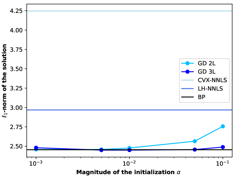
(a) Initialization.

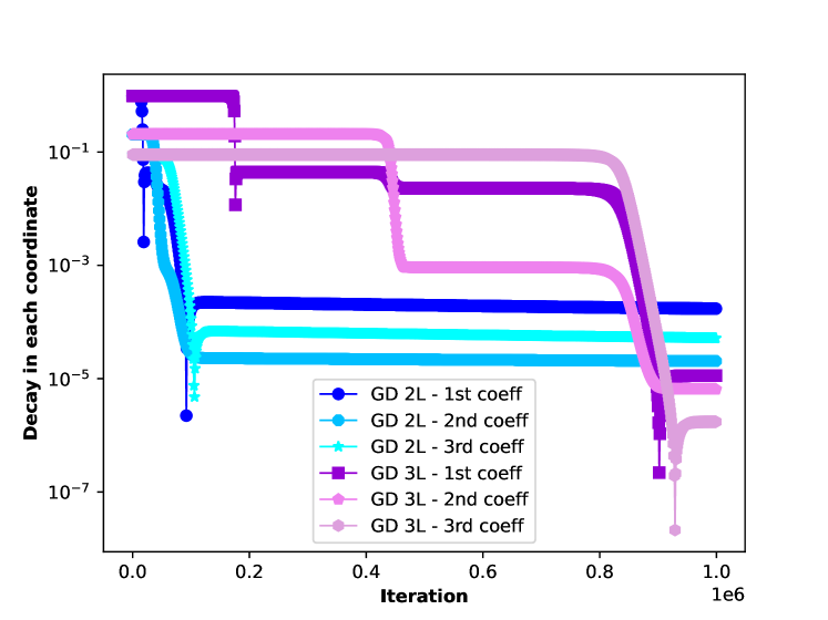
(b) Number of layers.

Figure 1: Influence of initialization, cf. Section 4.1, and number of layers on GD-$n$L, cf. Section 4.2.

4.2 Number of layers

In the second experiment, we take a closer look at the reconstruction behavior of GD-$n$L. In particular, we compare how different entries of the ground-truth are approximated over time, for $n=2$ and $n=3$ layers. For initialization magnitude and step-size we choose $\alpha=10^{-2}$ and $\eta=10^{-2}$. We set $M=30$ and $N=50$, draw a random Gaussian matrix ${\bf A}\in\mathbb{R}^{M\times N}$, create a $3$-sparse non-negative ground-truth ${\bf x}\in\mathbb{R}^{N}$, and set ${\bf y}={\bf A}{\bf x}$. Note that ${\bf A}$ satisfies the assumptions of Theorem 2.7. Figure 1(b) depicts the entry-wise error between the three non-zero ground-truth entries and the corresponding entries of the iterates of GD-$2$L and GD-$3$L. As already observed in previous related works, we see that a deeper factorization leads to sharper error transitions that occur later and that more dominant entries are recovered faster than the rest. Interestingly, there occurs some kind of overshooting in the dominant entries. The dark blue and purple curves suggest that GD-$n$L does not monotonically decrease the error in all components but rather concentrates heavily on the leading component(s) in the beginning and only starts distributing the error over time. In this way, GD-$n$L could be interpreted as a self-correcting greedy method.

4.3 Different stepsizes

In the third experiment, we compare the convergence rates of GD-$n$L and SGD-$n$L for various choices of step-size. Apart from using a constant step-size $\eta>0$, we also consider Nesterov acceleration [55] and the BB stepsize rules [30, 62]. Figure 2 shows the decay in training error, i.e., objective value over time in two different settings: the dense case, i.e., we have a quadratic system with $M=N=50$ and a dense ground-truth, and the sparse case, i.e., we have an underdetermined system with $M=30$, $N=50$, and a $3$-sparse ground-truth. In both settings ${\bf A}$ has Gaussian entries. As Figures 2(a) and 2(b) show, advanced choices of step-size notably improve the convergence rate of the gradient methods. Moreover, GD-$n$L seems to profit more from the acceleration than SGD-$n$L.

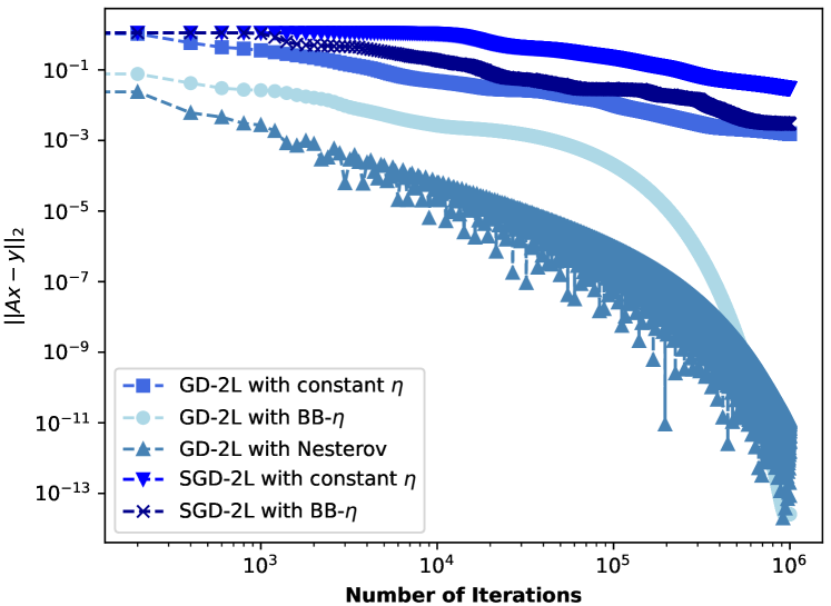
(a) Dense case

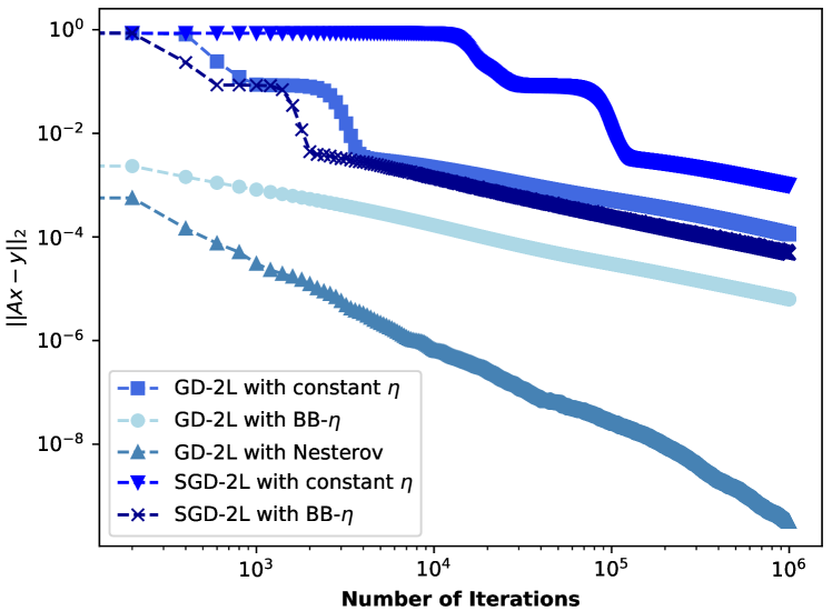
(b) Sparse case

Figure 2: Convergence rate for various choices of step-size, see Section 4.3.

4.4 Stability with Negative Entries

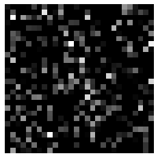
(a) HL-NNLS
($q=0.5$)

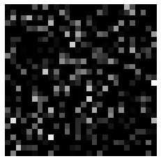
(b) TNT-NN
($q=0.5$)

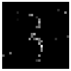
(c) SGD-3L
($q=0.5$)

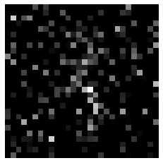
(d) GD-3L
($q=0.5$)

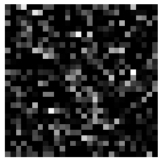
(e) PGD
($q=0.5$)

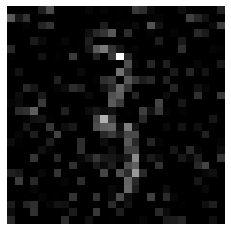
(f) HL-NNLS
($q=0.05$)

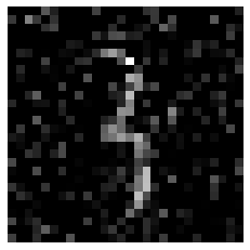
(g) TNT-NN
($q=0.05$)

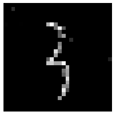
(h) SGD-3L
($q=0.05$)

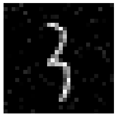
(i) GD-3L
($q=0.05$)

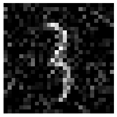
(j) PGD
($q=0.05$)

Figure 3: Illustration of the MNIST reconstruction, see Section 4.4.

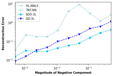
(a) Gaussian.

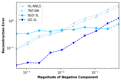
(b) MNIST.

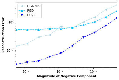
(c) MNIST with PGD.

Figure 4: Comparison of stability, see Section 4.4.

In our final experiment, we compare the stability of the proposed methods when recovering perturbed signals that are not strictly non-negative anymore. We consider two different set-ups. First, we create generic random signals and, second, we use signals from the MNIST data set representing real-world data. In both scenarios we set $\alpha=10^{-2}$ and $\eta=10^{-2}$ for GD-$n$L and SGD-$n$L. It is noteworthy that in all tested instances GD-$n$L and SGD-$n$L outperform the established methods in reconstruction quality, cf. Figure 3. Whereas HL-NNLS and TNT-NN are designed to retrieve only non-negative signals, the gradient based methods can stably deal with vectors that have small negative components by not using explicit constraints.

Gaussian signals

Let ${\bf A}\in\mathbb{R}^{M\times N}$ be a random Gaussian matrix, where $M=30$ and $N=50$. We pick a $3$-sparse non-negative vector ${\bf x}_{+}\in\mathbb{R}_{+}^{N}$ at random. We, furthermore, define a noise vector ${\bf x}_{-}\in\mathbb{R}_{+}^{N}$ that is $0$ on the support of ${\bf x}_{+}$ and has positive Gaussian entries everywhere else. For $q\in[0,1]$, we scale ${\bf x}_{+},{\bf x}_{-}$ such that

$$\|{\bf x}_{+}\|_{2}^{2}=1-q\quad\text{and}\quad\|{\bf x}_{-}\|_{2}^{2}=q.$$ (10)

The perturbed signal is then given by ${\bf x}={\bf x}_{+}-{\bf x}_{-}$ and $q$ regulates the negative corruption. We regard the copy of ${\bf x}_{+}$ scaled to $\ell_{2}$-norm $(1-q)$ as ground-truth and, by abuse of notation, also refer to it as ${\bf x}_{+}$. The corresponding measurements are given as ${\bf y}={\bf A}{\bf x}={\bf A}({\bf x}_{+}-{\bf x}_{-})$.

MNIST signals

Again ${\bf A}\in\mathbb{R}^{M\times N}$ is a random Gaussian matrix, where now $M=300$ and $N=28^{2}=784$. We take ${\bf x}_{+}$ to be the original MNIST image (number three) and define a corrupted signal ${\bf x}$ including negative Gaussian noise ${\bf x}_{-}$ as in (10), for $q\in[0,1]$. Note that our ground-truth is again a re-scaled version of the original image that has $\ell_{2}$-norm $(1-q)$.
Figures 4(a), 4(b) and 4(c) compare the reconstruction error $\|\hat{\bf x}-{\bf x}_{+}\|_{2}$ of HL-NNLS, TNT-NN, GD-$3$L, and SGD-$3$L over various choices of $q$. Here we set $\alpha=10^{-2}$ and $\eta=10^{-2}$. These figures clearly show that the gradient descent based methods outperform the established NNLS solvers. Only for small negative noise levels and MNIST data SGD-$3$L yields worse results than HL-NNLS and TNT-NN. As can be seen from Figure 3, this worse error is mainly caused by incorrect values on the support of ${\bf x}_{+}$. Visually, even for small $q$, the MNIST reconstruction of SGD-$3$L is far better than the one of HL-NNLS and TNT-NN.
The experiment also reveals two interesting points. First, whereas it has numerically been observed in [59] that, compared to gradient descent, stochastic gradient descent reduces the generalization (resp. approximation) error if measured in $\ell_{2}$-norm, we observe this (in the case of NNLS) only for large values of $q$, i.e., strong negative perturbations. For small values of $q$, Figure 2 rather suggests that GD-$3$L outperforms SGD-$3$L. Second, for all values of $q$ the solutions computed by SGD-$3$L are visually closer to the ground-truth than the ones computed by GD-$3$L, cf. Figure 3. This suggests that, even in the simple context of sparse recovery, (i) the $\ell_{2}$-norm might not be the appropriate measure for the generalization error and (ii) the stochasticity in SGD-$3$L apparently improves the generalization quality. Formalizing and proving this observation is an appealing topic for future research.

5 Conclusion

In this paper we have shown that, due to its implicit bias, vanilla gradient flow/descent is a reliable and scalable solver for the decade-old problem of NNLS that, in contrast to many established methods, comes with strong theoretical guarantees. Whereas most works on the implicit bias of gradient descent focus on explaining the still mysterious success of deep learning, we see much potential in exploiting this phenomenon in other contexts and more classical problems as well. With the present paper we hope to initiate further research and discussion in this direction.

Appendix A Proofs of Theorems 2.1 and 2.3

Let us for convenience recall the statements of Theorems 2.1 and 2.3 before starting the proof. For simplicity, we merge both results into a single statement.

Theorem A.1.

Let $L\geq 2$, ${\bf A}\in\mathbb{R}^{M\times N}$ and ${\bf y}\in\mathbb{R}^{M}$. Define the overparameterized loss function $\mathcal{L}_{\text{over}}$ as

$$\mathcal{L}_{\text{over}}\big{(}{\bf x}^{(1)},\dots,{\bf x}^{(L)}\big{)}:=\frac{1}{2}\,\|{\bf A}\tilde{\bf x}-{\bf y}\|_{2}^{2}$$ (11)

where $\tilde{\bf x}={\bf x}^{(1)}\odot\cdots\odot{\bf x}^{(L)}$. Let ${\bf x}_{0}>\bm{0}$ be fixed and, for any $k$, let ${\bf x}^{(k)}(t)$ follow the flow $\big{(}{\bf x}^{(k)}\big{)}^{\prime}(t)=-\nabla_{{\bf x}^{(k)}}\mathcal{L}_{\text{over}}$ with ${\bf x}^{(k)}(0)={\bf x}_{0}$. Let $S_{+}$ be the set defined in (NNLS). Then the limit $\tilde{{\bf x}}_{\infty}:=\lim_{t\to\infty}\tilde{\bf x}(t)$ exists and lies in $S_{+}$.

Let $\varepsilon>0$ and assume in addition that ${\bf x}_{0}=\alpha{\bf 1}$. If

$$\alpha\leq h(Q_{+},\varepsilon):=\begin{cases}\exp\left(-\frac{1}{2}-\frac{Q_{+}^{2}+Ne^{-1}}{2\varepsilon}\right)&\text{if }L=2\\ \left(\frac{2\varepsilon}{L(Q_{+}+N+\varepsilon)}\right)^{\frac{1}{L-2}}&\text{if }L>2\end{cases},$$ (12)

where $Q_{+}=\min_{{\bf z}\in S_{+}}\|{\bf z}\|_{1}$, then the $\ell_{1}$-norm of $\tilde{{\bf x}}_{\infty}$ satisfies

$$\|\tilde{{\bf x}}_{\infty}\|_{1}-\min_{{\bf z}\in S_{+}}\|{\bf z}\|_{1}\leq\varepsilon.$$

The proof consists of three major steps: First, the objective function and the corresponding flow are reduced to a simplified form by using the fact that all factors are initialized identically. Second, we prove that the reduced flow converges and characterize its limits as the minimizer of a specific optimization problem. Finally, we show that if ${\bf x}_{0}=\alpha{\bf 1}$, the limit approximately minimizes the $\ell_{1}$-norm among all possible solutions of (NNLS). Whereas the first and the third step are taken unchanged from [21], the second step, which is the backbone of the argument, requires a different reasoning due to the (possible) non-existence of solutions ${\bf A}{\bf z}={\bf y}$. Let us now start with the proof.

As already mentioned, we use the same reduction as in [21] to analyze the dynamics ${\bf x}^{\prime}(t)=-\nabla\mathcal{L}_{\text{over}}$.

Lemma A.2 (Identical Initialization, [21, Lemma 2.3]).

Suppose ${\bf x}^{(k)}(t)$ follows the negative gradient flow

$$\left({\bf x}^{(k)}\right)^{\prime}(t)=-\nabla_{{\bf x}^{(k)}}\mathcal{L}_{\text{over}}\big{(}{\bf x}^{(1)},\dots,{\bf x}^{(L)}\big{)}\;.$$

If all initialization vectors are identical, i.e. ${\bf x}^{(k)}(0)={\bf x}^{(k^{\prime})}(0)$ for all $k,k^{\prime}\in[L]$, then the vectors remain identical for all $t\geq 0$, i.e. ${\bf x}^{(k)}(t)={\bf x}^{(k^{\prime})}(t)$. Moreover, the dynamics will be given by

$${\bf x}^{\prime}(t)=-\nabla\mathcal{L}({\bf x})\;.$$

where ${\bf x}={\bf x}^{(1)}=\dots={\bf x}^{(L)}$ and $\mathcal{L}({\bf x})=\frac{1}{2}\|{\bf A}{\bf x}^{\odot L}-{\bf y}\|_{2}^{2}$.

Based on Lemma A.2, we can restrict ourselves to a simplified loss in the following.

Definition A.3 (Reduced Factorized Loss, [21, Definition 2.4]).

Let $L\in\mathbb{N}$, $L\geq 2$. For ${\bf A}\in\mathbb{R}^{M\times N}$ and ${\bf y}\in\mathbb{R}^{M}$, the reduced factorized loss function is defined as

$$\mathcal{L}\colon\mathbb{R}^{N}\to[0,\infty),\qquad\mathcal{L}({\bf x}):=\frac{1}{2}\|{\bf A}{\bf x}^{\odot L}-{\bf y}\|_{2}^{2}.$$ (13)

Its derivative is given by $\nabla\mathcal{L}({\bf x})=\left[{\bf A}^{\text{T}}({\bf A}{\bf x}^{\odot L}-{\bf y})\right]\odot{\bf x}^{\odot L-1}$.

In order to prove that ${\bf x}^{\odot L}$ converges to an element in $S_{+}$ defined in (NNLS), we use the concept of Bregman divergence.

Definition A.4 (Bregman Divergence).

Let $F:\Omega\to\mathbb{R}$ be a continuously-differentiable, strictly convex function defined on a closed convex set $\Omega$. The Bregman divergence associated with $F$ for points $p,q\in\Omega$ is defined as

$$D_{F}(p,q)=F(p)-F(q)-\langle\nabla F(q),p-q\rangle.$$ (14)

Lemma A.5 ([10]).

The Bregman divergence $D_{F}$ is non-negative and strictly convex in $p$.

We can now show convergence of ${\bf x}(t)^{\odot L}$ and characterize its limit.

Theorem A.6.

Let $\tilde{\bf x}(t)={\bf x}(t)^{\odot L}$ and

$${\bf x}^{\prime}(t)=-\nabla\mathcal{L}({\bf x}(t))=-\left[{\bf A}^{\text{T}}({\bf A}{\bf x}^{\odot L}(t)-{\bf y})\right]\odot{\bf x}^{\odot L-1}(t)$$ (15)

with ${\bf x}(0)\geq 0$. Then $\tilde{{\bf x}}_{\infty}:=\lim_{t\to\infty}\tilde{\bf x}(t)$ exists and

$$\tilde{{\bf x}}_{\infty}=\operatorname*{arg\,min}_{{\bf z}\in S_{+}}g_{\tilde{\bf x}(0)}({\bf z}):=\operatorname*{arg\,min}_{{\bf z}\in S_{+}}\begin{cases}\langle{\bf z},\log({\bf z})-{\bf 1}-\log(\tilde{\bf x}(0))\rangle&\text{if }L=2\\ 2\|{\bf z}\|_{1}-L\langle{\bf z}^{\odot\frac{2}{L}},\tilde{\bf x}(0)^{\odot(1-\frac{2}{L})}\rangle&\text{if }L>2.\end{cases}$$ (16)

where $S_{+}$ is defined in (NNLS).

Theorem A.6 resembles [21, Theorem 2.7]. Note, however, that the definition of $S_{+}$ is different and that Theorem A.6 does not require the existence of a solution of ${\bf A}{\bf x}={\bf y}$.

To prove Theorem A.6, we use the same $F:\mathbb{R}_{\geq 0}^{N}\to\mathbb{R}$ as in [21], i.e.,

$$F({\bf x})=\begin{cases}\frac{1}{2}\langle{\bf x}\log({\bf x})-{\bf x},\bm{1}\rangle&\text{if }L=2\\ \frac{L}{2(2-L)}\langle{\bf x}^{\odot\frac{2}{L}},\bm{1}\rangle&\text{if }L>2\end{cases}=\begin{cases}\frac{1}{2}\sum_{n=1}^{N}x_{n}\log(x_{n})-x_{n}&\text{if }L=2\\ \frac{L}{2(2-L)}\sum_{n=1}^{N}x_{n}^{\frac{2}{L}}&\text{if }L>2,\end{cases}$$ (17)

where we set $0\log(0)=\lim_{z\to 0}z\log(z)=0$. Note that $F$ is strictly convex because its Hessian $\mathbf{H}_{F}({\bf x})$ is diagonal with positive diagonal entries $\frac{1}{L}x_{n}^{-2+\frac{2}{L}}$. Thus the Bregman divergence $D_{F}$ is well-defined and has the following property.

Lemma A.7 ([21, Lemma 2.8]).

Let $F$ be the function defined in (17), ${\bf z}\geq\bm{0}$ be fixed, and ${\bf x}(t)\colon\mathbb{R}_{\geq 0}\to\mathbb{R}_{\geq 0}^{N}$ be a continuous function with ${\bf x}(0)>\bm{0}$ and $\|{\bf x}(t)\|_{2}\to\infty$. Then $D_{F}({\bf z},{\bf x}(t))\to\infty$.

In addition, we require the following geometric observation.

Lemma A.8.

Let $C\subset\mathbb{R}^{n}$ be a convex and closed set. Let ${\bf w}\in C$, ${\bf y}\in\mathbb{R}^{n}$ with ${\bf y}\neq{\bf w}$, and let $\mathcal{P}_{C}{\bf y}$ denote the (unique) Euclidean projection of ${\bf y}$ onto $C$. Then

$$\langle{\bf w}-{\bf y},{\bf w}-\mathcal{P}_{C}{\bf y}\rangle\geq\frac{1}{2}\|{\bf w}-\mathcal{P}_{C}{\bf y}\|_{2}^{2}.$$ (18)

Furthermore, it holds that

$$\|{\bf w}-\mathcal{P}_{C}{\bf y}\|_{2}^{2}\leq\|{\bf w}-{\bf y}\|_{2}^{2}-\|{\bf y}-\mathcal{P}_{C}{\bf y}\|_{2}^{2}.$$

Proof.

By definition of the projection, we have that

$$\|{\bf w}-{\bf y}\|_{2}^{2}\geq\|\mathcal{P}_{C}{\bf y}-{\bf y}\|_{2}^{2} =\|-({\bf w}-\mathcal{P}_{C}{\bf y})+{\bf w}-{\bf y}\|_{2}^{2}$$

$$=\|{\bf w}-\mathcal{P}_{C}{\bf y}\|_{2}^{2}-2\langle{\bf w}-\mathcal{P}_{C}{\bf y},{\bf w}-{\bf y}\rangle+\|{\bf w}-{\bf y}\|_{2}^{2}.$$

Rearranging the terms yields

$$2\langle{\bf w}-{\bf y},{\bf w}-\mathcal{P}_{C}{\bf y}\rangle\geq\|{\bf w}-\mathcal{P}_{C}{\bf y}\|_{2}^{2}$$

and thus the first claim. Now note that $\langle{\bf w}-\mathcal{P}_{C}{\bf y},{\bf y}-\mathcal{P}_{C}{\bf y}\rangle\leq 0$ by $\mathcal{P}_{C}$ being a convex projection, e.g., see [13, Lemma 3.1]. This yields

$$\|{\bf w}-{\bf y}\|_{2}^{2} =\|{\bf w}-\mathcal{P}_{C}{\bf y}-({\bf y}-\mathcal{P}_{C}{\bf y})\|_{2}^{2}$$

$$=\|{\bf w}-\mathcal{P}_{C}{\bf y}\|_{2}^{2}-2\langle{\bf w}-\mathcal{P}_{C}{\bf y},{\bf y}-\mathcal{P}_{C}{\bf y}\rangle+\|{\bf y}-\mathcal{P}_{C}{\bf y}\|_{2}^{2}$$

$$\geq\|{\bf w}-\mathcal{P}_{C}{\bf y}\|_{2}^{2}+\|{\bf y}-\mathcal{P}_{C}{\bf y}\|_{2}^{2}$$

and thus the second claim. ∎

With these tools at hand, we can prove Theorem A.6.

Proof of Theorem A.6.

Let us begin with a brief outline of the proof. We will first compute the time derivative of $D_{F}({\bf z}_{+},\tilde{\bf x}(t))$, for ${\bf z}_{+}\in S_{+}$ where $S_{+}$ was defined in (NNLS). These first steps appeared before in the proof of [21, Theorem 2.7] and are only detailed for the reader’s convenience. With help of Lemma A.8 we can then show that ${\bf A}\tilde{\bf x}(t)\to{\bf y}_{+}$. This part of the proof requires more work than in [21] due to the possible non-existence of pre-images for ${\bf y}$ under ${\bf A}$. The final steps (deducing boundedness and convergence of $\|\tilde{\bf x}(t)\|_{2}$ via Lemma A.7 and characterizing the limit $\tilde{{\bf x}}_{\infty}$) are then taken again from [21]. Only the definition of the set $S_{+}$ is different.

We start with computing $\partial_{t}D_{F}({\bf z},\tilde{\bf x}(t))$. If any entry $x(t)_{i}$ vanishes at $t_{*}>0$, then $x(t)_{i}=0$ for all $t\geq t_{*}$ by the shape of (15). Hence, by continuity ${\bf x}(t)\geq 0$ for all $t\geq 0$. For any ${\bf z}\in\mathbb{R}^{N}$, we have

$$\partial_{t}D_{F}({\bf z},\tilde{\bf x}(t)) =\partial_{t}\left[F({\bf z})-F(\tilde{\bf x}(t))-\langle\nabla F(\tilde{\bf x}(t)),{\bf z}-\tilde{\bf x}(t)\rangle\right]$$

$$=0-\langle\nabla F(\tilde{\bf x}(t)),\tilde{\bf x}^{\prime}(t)\rangle-\langle\partial_{t}\nabla F(\tilde{\bf x}(t)),{\bf z}-\tilde{\bf x}(t)\rangle+\langle\nabla F(\tilde{\bf x}(t)),\tilde{\bf x}^{\prime}(t)\rangle$$

$$=-\langle\partial_{t}\nabla F(\tilde{\bf x}(t)),{\bf z}-\tilde{\bf x}(t)\rangle.$$

By the chain rule and the diagonal shape of $\mathbf{H}_{F}$, we calculate that

$$\partial_{t}\nabla F(\tilde{\bf x}(t)) =\mathbf{H}_{F}(\tilde{\bf x}(t))\cdot\tilde{\bf x}^{\prime}(t)=\frac{1}{L}\tilde{\bf x}(t)^{\odot(-2+\frac{2}{L})}\odot\tilde{\bf x}^{\prime}(t)=\frac{1}{L}{\bf x}(t)^{\odot(-2L+2)}\odot\big{(}L{\bf x}(t)^{\odot(L-1)}\odot{\bf x}^{\prime}(t)\big{)}$$

$$={\bf x}(t)^{\odot(-2L+2)}\odot{\bf x}(t)^{\odot(L-1)}\odot\big{(}-\left[{\bf A}^{\text{T}}({\bf A}{\bf x}^{\odot L}(t)-{\bf y})\right]\odot{\bf x}^{\odot L-1}(t)\big{)}$$

$$=-\left[{\bf A}^{\text{T}}({\bf A}\tilde{\bf x}(t)-{\bf y})\right]$$

By definition, it is clear that $S_{+}\neq\emptyset$. Let ${\bf z}_{+}$ be any element of $S_{+}$. Since $C_{+}=\{{\bf A}{\bf z}\colon{\bf z}\in\mathbb{R}_{\geq 0}\}\subset\mathbb{R}^{M}$ is a closed convex set and ${\bf y}_{+}=\mathbb{P}_{C_{+}}{\bf y}$, we can set $C=C_{+}$, ${\bf w}={\bf A}\tilde{\bf x}(t)\in C_{+}$, and ${\bf y}={\bf y}$ in Lemma A.8 and obtain that

$$\begin{split}\partial_{t}D_{F}({\bf z}_{+},\tilde{\bf x}(t))&=-\langle{\bf A}\tilde{\bf x}(t)-{\bf y},{\bf A}\tilde{\bf x}(t)-{\bf A}{\bf z}_{+}\rangle\\ &\leq-\frac{1}{2}\|{\bf A}\tilde{\bf x}(t)-{\bf y}_{+}\|_{2}^{2}.\end{split}$$ (19)

Note that $D_{F}({\bf z}_{+},\tilde{\bf x}(t))$ must converge for $t\to\infty$ as it is bounded from below and monotonically decreasing ($D_{F}({\bf z}_{+},\tilde{\bf x}(t))\geq 0$ and $\partial_{t}D_{F}({\bf z}_{+},\tilde{\bf x}(t))~{}\leq~{}0$). In particular, $0\leq D_{F}({\bf z}_{+},\tilde{\bf x}(t))\leq D_{F}({\bf z}_{+},\tilde{\bf x}(0))$ for all $t\geq 0$.

We now show that ${\bf A}\tilde{\bf x}(t)\to{\bf y}_{+}$ with the given rate. Recall that ${\bf z}_{+}$ is any element in $S_{+}$ and note that by (19)

$$C :=D_{F}({\bf z}_{+},\tilde{\bf x}(0))\geq D_{F}({\bf z}_{+},\tilde{\bf x}(0))-D_{F}({\bf z}_{+},\tilde{\bf x}(T))=-\int_{0}^{T}\partial_{t}D_{F}({\bf z}_{+},\tilde{\bf x}(t))dt$$

$$\geq\frac{1}{2}\int_{0}^{T}\|{\bf A}\tilde{\bf x}(t)-{\bf y}_{+}\|_{2}^{2}dt\geq\frac{T}{2}\min_{t\in[0,T]}\|{\bf A}\tilde{\bf x}(t)-{\bf y}_{+}\|_{2}^{2},$$

for any $T>0$. This implies that, for any $T$, there exists a $t_{T}\in[0,T]$ with $\|{\bf A}\tilde{\bf x}(t_{T})-{\bf y}_{+}\|_{2}^{2}\leq\frac{2C}{T}$. Since

$$\|{\bf A}\tilde{\bf x}(t_{T})-{\bf y}\|_{2}\leq\|{\bf A}\tilde{\bf x}(t_{T})-{\bf y}_{+}\|_{2}+\|{\bf y}-{\bf y}_{+}\|_{2}\leq\frac{2C}{T}+\|{\bf y}-{\bf y}_{+}\|_{2},$$

we can apply Lemma A.8 once more (by setting $C=C_{+}$, ${\bf w}={\bf A}\tilde{\bf x}(T)\in C_{+}$, and ${\bf y}={\bf y}$) to obtain that

$$\|{\bf A}\tilde{\bf x}(T)-{\bf y}_{+}\|_{2}^{2} \leq\|{\bf A}\tilde{\bf x}(T)-{\bf y}\|_{2}^{2}-\|{\bf y}-{\bf y}_{+}\|_{2}^{2}\leq\|{\bf A}\tilde{\bf x}(t_{T})-{\bf y}\|_{2}^{2}-\|{\bf y}-{\bf y}_{+}\|_{2}^{2}$$

$$\leq\frac{4C^{2}}{T^{2}}+\frac{2C}{T}\|{\bf y}-{\bf y}_{+}\|_{2}^{2}=\mathcal{O}\Big{(}\frac{1}{T}\Big{)},$$

where we used in the second step that the loss function is monotonically decreasing in time along the trajectory. In particular, this shows that $\lim_{t\to\infty}{\bf A}\tilde{\bf x}(t)={\bf y}_{+}$.

Using Lemma A.7, boundedness of $\|\tilde{\bf x}(t)\|_{2}$ follows as in [21]. Just fix any ${\bf z}_{+}\in S_{+}$ and notice that $D_{F}({\bf z}_{+},\tilde{\bf x}(t))\to\infty$ if $\|\tilde{\bf x}(t)\|_{2}\to\infty$ which contradicts the fact that $0\leq D_{F}({\bf z}_{+},\tilde{\bf x}(t))\leq D_{F}({\bf z}_{+},\tilde{\bf x}(0))$. Let us denote by $B$ a sufficiently large compact ball around the origin such that $B\cap S_{+}\neq\emptyset$ and $\tilde{\bf x}(t)\in B$, for all $t\geq 0$.

Now assume that there exists no ${\bf z}_{+}\in S_{+}\cap B$ such that $\lim_{t\to\infty}D_{F}({\bf z}_{+},\tilde{\bf x}(t))=0$, i.e., by compactness of $S_{+}\cap B$ there exists $\varepsilon>0$ such that $\lim_{t\to\infty}D_{F}({\bf z}_{+},\tilde{\bf x}(t))>\varepsilon$, for all ${\bf z}_{+}\in S_{+}\cap B$. By strict convexity of $D_{F}(\cdot,\tilde{\bf x}(t))$, this implies that $\tilde{\bf x}$ is bounded away from the set $S_{+}$ on $B$ and $\|{\bf A}\tilde{\bf x}(t)-{\bf y}_{+}\|_{2}$ cannot converge to zero contradicting the just obtained convergence $\lim_{t\to\infty}{\bf A}\tilde{\bf x}(t)={\bf y}_{+}$. Hence, there exists ${\bf z}_{+}\in S_{+}$ with $\lim_{t\to\infty}D_{F}({\bf z}_{+},\tilde{\bf x}(t))=0$.

For any such ${\bf z}_{+}$, let us assume that $\tilde{\bf x}(t)\nrightarrow{\bf z}_{+}$. Then there exists $\varepsilon>0$ and a sequence of times $t_{0},t_{1},\dots$ with $\|{\bf z}_{+}-\tilde{\bf x}(t_{k})\|_{2}\geq\varepsilon$ and $\lim_{k\to\infty}D_{F}({\bf z}_{+},\tilde{\bf x}(t_{k}))=0$. Since $\tilde{\bf x}(t_{k})$ is a bounded sequence, a (not relabeled) subsequence converges to some $\bar{{\bf x}}$ with $\|{\bf z}_{+}-\bar{{\bf x}}\|_{2}\geq\varepsilon$ and $D_{F}({\bf z}_{+},\bar{{\bf x}})=0$. Since $D_{F}(\bar{{\bf x}},\bar{{\bf x}})=0$ and $D_{F}$ is non-negative, this is a contradiction to the strict convexity of $D_{F}(\cdot,\bar{{\bf x}})$. Hence, $\tilde{\bf x}_{\infty}=\lim_{t\to\infty}\tilde{\bf x}(t)\in S_{+}$ exists and is the unique solution satisfying $\lim_{t\to\infty}~{}D_{F}~{}(\tilde{\bf x}_{\infty},\tilde{\bf x}(t))~{}=~{}0$.

Because $\partial_{t}D_{F}({\bf z}_{+},\tilde{\bf x}(t))$ is identical for all ${\bf z}_{+}\in S_{+}$ (the second line of (19) does not depend on the choice of ${\bf z}_{+}$), the difference

$$\Delta_{{\bf z}_{+}}=D_{F}({\bf z}_{+},\tilde{\bf x}(0))-D_{F}({\bf z}_{+},\tilde{{\bf x}}_{\infty})$$ (20)

is also identical for all ${\bf z}_{+}\in S_{+}$. By non-negativity of $D_{F}$,

$$D_{F}({\bf z}_{+},\tilde{\bf x}(0))\geq\Delta_{{\bf z}_{+}}=\Delta_{\tilde{{\bf x}}_{\infty}}=D_{F}(\tilde{{\bf x}}_{\infty},\tilde{\bf x}(0)).$$ (21)

Thus

$$\tilde{{\bf x}}_{\infty}\in \operatorname*{arg\,min}_{{\bf z}\in S_{+}}D_{F}({\bf z},\tilde{\bf x}(0))$$

$$=\operatorname*{arg\,min}_{{\bf z}\in S_{+}}F({\bf z})-F(\tilde{\bf x}(0))-\langle\nabla F(\tilde{\bf x}(0)),{\bf z}-\tilde{\bf x}(0)\rangle$$

$$=\operatorname*{arg\,min}_{{\bf z}\in S_{+}}F({\bf z})-\langle\nabla F(\tilde{\bf x}(0)),{\bf z}\rangle$$

$$=\operatorname*{arg\,min}_{{\bf z}\in S_{+}}\begin{cases}\sum_{n=1}^{N}z_{n}\log(z_{n})-z_{n}-\log(\tilde{x}_{n}(0))z_{n}&\text{if }L=2\\ \sum_{n=1}^{N}-z_{n}^{\frac{2}{L}}+\frac{2}{L}\tilde{x}_{n}(0)^{-1+\frac{2}{L}}z_{n}&\text{if }L>2\end{cases}$$

$$=\operatorname*{arg\,min}_{{\bf z}\in S_{+}}\begin{cases}\langle{\bf z},\log({\bf z})-{\bf 1}-\log(\tilde{\bf x}(0))\rangle&\text{if }L=2\\ 2\|{\bf z}\|_{1}-L\langle{\bf z}^{\frac{2}{L}},\tilde{\bf x}(0)^{1-\frac{2}{L}}\rangle&\text{if }L>2.\end{cases}$$

∎

Proof of Theorem A.1.

By Lemma A.2, the assumption that ${\bf x}^{(k)}(0)={\bf x}^{(k^{\prime})}(0)$, for all $k,k^{\prime}\in[L]$, implies that ${\bf x}^{(k)}(t)={\bf x}^{(k^{\prime})}(t)$, for all $t\geq 0$. Furthermore, each ${\bf x}^{(k)}(t)$ equals ${\bf x}(t)$ defined via ${\bf x}(0)={\bf x}^{(k)}(0)$ and ${\bf x}^{\prime}(t)=-\nabla\mathcal{L}({\bf x})$. By Theorem A.6, the limit ${\bf x}_{\infty}:=\lim_{t\to\infty}{\bf x}(t)$ exists and $\tilde{{\bf x}}_{\infty}={\bf x}_{\infty}^{\odot L}$ lies in $S_{+}$. Let ${\bf z}\in S_{+}$, i.e., is an admissible solution to (NNLS). The quantitative bound in (12) can easily be deduced by following the steps in [21] since (16) and [21, Equation (18)] are identical up to the definition of $S_{+}$. ∎

Appendix B Proof of Remark 2.2

Since the problem (NNLS) is convex, the Karush-Kuhn-Tucker (KKT) conditions are necessary and sufficient for optimality, see, e.g., [9].

Theorem B.1.

(Karush-Kuhn-Tucker conditions for NNLS) A point ${\bf x}_{+}\in\mathbb{R}^{N}$ is a solution of problem (NNLS) if and only if there exists $\mathbf{w}^{\star}\in\mathbb{R}^{n}$ and a partition $A\cup P=\left\{1,\dots,N\right\}$ such that

$$\mathbf{w}^{\star}={\bf A}^{T}(\mathbf{y}-{\bf A}{\bf x}_{+}),$$ (22)

$$(x_{+})_{i}=0,\ i\in A,\quad(x_{+})_{i}>0,\ i\in P,$$ (23)

$$w^{\star}_{i}\leq 0,\ i\in A,\quad w^{\star}_{i}=0,\ i\in P.$$ (24)

The equations (23-24) imply

$$(x_{+})_{i}w^{\star}_{i}=0,\ i=1,\dots,N,$$ (25)

which are the KKT complementarity conditions.

From these conditions, one can observe that all solutions of (NNLS) can be represented by stationary points of the functional

$$\mathcal{L}_{\text{over}}\big{(}{\bf x}^{(1)},\dots,{\bf x}^{(L)}\big{)}:=\frac{1}{2}\,\Big{\|}{\bf A}\big{(}{\bf x}^{(1)}\odot\cdots\odot{\bf x}^{(L)}\big{)}-{\bf y}\Big{\|}_{2}^{2}$$

in (4), i.e., points that satisfy, for all $\ell\in[L]$, the equation

$$\nabla L_{{\bf x}^{(\ell)}}\big{(}{\bf x}^{(1)},\dots,{\bf x}^{(L)}\big{)}=\left[{\bf A}^{\text{T}}\Big{(}{\bf A}\big{(}{\bf x}^{(1)}\odot\cdots\odot{\bf x}^{(L)}\big{)}-{\bf y}\Big{)}\right]\odot\Big{(}\bigodot_{k\neq\ell}{\bf x}^{(k)}\Big{)}=\bm{0}.$$ (26)

Indeed, for any given optimal point $\mathbf{x}_{+}$ of the (NNLS) problem, it is straight-forward to check that the conditions in Theorem B.1 imply that ${\bf x}^{(1)}=\cdots={\bf x}^{(L)}={\bf x}_{+}^{\odot\frac{1}{L}}$ is a stationary point of (4) with ${\bf x}^{(1)}\odot\cdots\odot{\bf x}^{(L)}={\bf x}_{+}$. The same argument holds for stationary points of the reduced functional (13). In particular, this implies that any solution of (NNLS) can be described as the limit of gradient flow on (4) under suitably chosen identical initialization.

Appendix C Proof of Remark 2.4

The statement in Remark 2.4 can be deduced from Theorem C.1 below by noticing that, for $L=2$, the initialization vector ${\bf x}_{0}$ defined as

$$(x_{0})_{i}=e^{-\frac{1}{2}(1+\theta w_{i})}$$

satisfies ${\bf w}=\frac{(-1-\log(\tilde{\bf x}(0)))}{\max_{n\in[N]}(-1-\log((\tilde{x}(0))_{n})}$ (recall that $\tilde{\bf x}(0)={\bf x}_{0}^{\odot 2}$ in this case). The scaling $\theta>0$, which has no effect on ${\bf w}$, only has to be chosen sufficiently large to guarantee ${\bf x}_{0}\leq h(Q_{+},\varepsilon)$.

Theorem C.1.

Let $\varepsilon>0$ and $L=2$. Under the assumptions of Theorem 2.3 with ${\bf x}_{0}\leq\alpha\leq h(Q_{+},\varepsilon)$, we get that

$$\|\tilde{{\bf x}}_{\infty}\|_{{\bf w},1}-\min_{{\bf z}\in S_{+}}\|{\bf z}\|_{{\bf w},1}\leq\varepsilon,$$

where $\|{\bf z}\|_{{\bf w},1}=\|{\bf z}\odot{\bf w}\|_{1}$ denotes the weighted $\ell_{1}$-norm for

$${\bf w}=\delta(-{\bf 1}-\log(\tilde{\bf x}_{0}))$$

and

$$\delta=\frac{1}{\max_{n\in[N]}(-1-\log((\tilde{x}_{0})_{n})}.$$

Proof.

For $L=2$, we obtain from (16) that

$$\tilde{{\bf x}}_{\infty}\in\operatorname*{arg\,min}_{{\bf z}\in S_{+}}\langle{\bf z},\log({\bf z})-{\bf 1}-\log(\tilde{\bf x}_{0})\rangle.$$

Hence

$$\langle\tilde{{\bf x}}_{\infty},\log(\tilde{{\bf x}}_{\infty})-{\bf 1}-\log(\tilde{\bf x}_{0})\rangle\leq\langle{\bf z},\log({\bf z})-{\bf 1}-\log(\tilde{\bf x}_{0})\rangle,$$

which may be re-stated as

$$\langle\tilde{{\bf x}}_{\infty}-{\bf z},-{\bf 1}-\log(\tilde{\bf x}_{0})\rangle\leq\langle{\bf z},\log({\bf z})\rangle-\langle\tilde{{\bf x}}_{\infty},\log(\tilde{{\bf x}}_{\infty})\rangle.$$

Let $\alpha\in(0,e^{-\frac{1}{2}})$ and assume that $\alpha\geq{\bf x}_{0}>0$ (so that $\log(\tilde{\bf x}_{0})<-1$). Note that $1\geq{\bf w}\geq 0$ by assumption. Denote

$$\|{\bf z}\|_{{\bf w},1}=\|{\bf z}\odot{\bf w}\|_{1}$$

to be the weighted $\ell_{1}$-norm. By non-negativity of ${\bf w},\tilde{{\bf x}}_{\infty},{\bf z}$, we get that

$$\|\tilde{{\bf x}}_{\infty}\|_{{\bf w},1}-\|{\bf z}\|_{{\bf w},1}\leq\delta(\langle{\bf z},\log({\bf z})\rangle-\langle\tilde{{\bf x}}_{\infty},\log(\tilde{{\bf x}}_{\infty})\rangle).$$

Since $\xi^{2}\geq\xi\log(\xi)\geq-e^{-1}$ for $\xi\geq 0$,

$$\|\tilde{{\bf x}}_{\infty}\|_{{\bf w},1}-\|{\bf z}\|_{{\bf w},1} \leq\delta(\|{\bf z}\|_{2}^{2}+Ne^{-1})\leq\delta(\|{\bf z}\|_{1}^{2}+Ne^{-1})\leq\varepsilon$$

because $\alpha\leq h(Q_{+},\varepsilon)$ and $\delta\leq-\frac{1}{1+2\log(\alpha)}$. Take the minimum over all ${\bf z}\in S_{+}$ and we get our conclusion. ∎

Appendix D Additional Numerical Experiments

In this section, we provide additional empirical evidence for our theoretical claims. In particular, (i) we illustrate the performance of our method in an over-determined large scale NNLS problem and (ii) we compare our method to projected gradient descent (PGD) [60] in terms of number of iterations, convergence rate, and running time since it is known that PGD converges linearly to the global minimizer [3, 60] and it is a numerically efficient method due to the fast calculation of the projection step.

D.1 Additional NNLS experiment on large scale

In this first experiment, cf. Figure 5, we illustrate the performance of our method for an overdetermined NNLS problem on a larger scale. The matrix ${\bf A}\in\mathbb{R}^{2048\times 1024}$ is standard Gaussian and, for a Gaussian random vector ${\bf x}\in\mathbb{R}^{1024}$, ${\bf y}$ is created as a perturbed version of ${\bf A}{\bf x}$ such that ${\bf y}$ is not in the range of ${\bf A}$. Furthermore, we use ${\bf x}_{0}=\bm{1}$ as a generic initialization. Figure 5 shows the error $\|{\bf A}{\bf x}^{\odot L}-{\bf y}\|_{2}$ over the iterations of gradient descent. As predicted by Theorem 2.1, our method converges to a solution that solves the NNLS problem (compare the error to the benchmark given by the Lawson-Hanson algorithm).

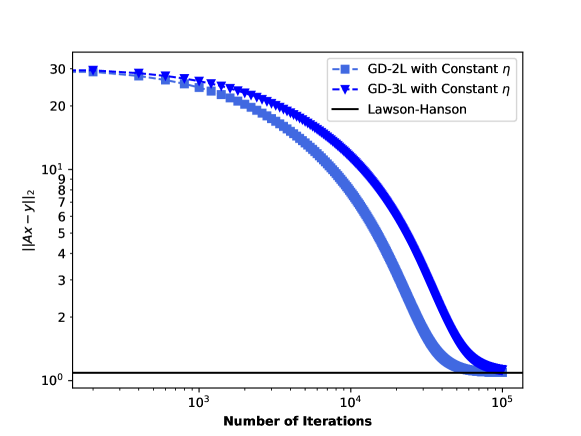
Figure 5: Large-scale NNLS problem, see Section D.1.

D.2 Comparison of averaged number of iterations

In the second experiment, cf. Figure 6, we illustrate the necessary amount of iterations to reach the precision $10^{-3}$. The matrix ${\bf A}\in\mathbb{R}^{512\times 1024}$ is a normalized $8$-sparse random vector ${\bf x}\in\mathbb{R}^{1024}$ with Gaussian entries that is made positive by considering only the absolute values of each entry, we generate ${\bf y}$ simply by doing ${\bf y}={\bf A}{\bf x}$, which means that we would expect the methods to converge to zero. We use ${\bf x}_{0}=\bm{1}$ as a generic initialization. As for the stepsize, for the PGD algorithm it was chosen as $\eta=1/L=1/||{\bf A}^{T}{\bf A}||_{2}$, the Lipschitz constant of the gradient. Also, for overparametrized GD-2L, overparametrized GD-3L and overparametrized SGD-2L, we choose a small but constant stepsize $\eta=0.02$. Moreover, we compare all of these methods against the GD-2L and GD-3L with the Barzilai-Borwein (BB) stepsize $\eta=\frac{||{\bf x}_{t}-{\bf x}_{t-1}||_{2}^{2}}{||{\bf A}({\bf x}_{t}-{\bf x}_{t-1})||_{2}^{2}}$[4]. We run it 100 times and take the median of the results in order to avoid outliers.

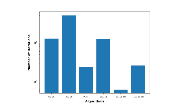
Figure 6: Comparison of the number of iterations, cf. Section D.2.

As expected, PGD shines as it is extremely fast for the convex formulation of NNLS and reaches good progress in the first $10^{3}$ iterations. Our non-convex formulation, on the other hand, needs more iterations to reach a very good precision. Nevertheless, by combining it with the BB stepsize, we manage to outperform the number of initial convergence of PGD. This illustrates the potential of further acceleration schemes that could leverage overparametrized formulations.

D.3 Running time comparison

In this experiment, we show a table with the necessary average running time, in seconds and averaged over 25 realizations, to run $10^{6}$ iteration of the NNLS problem for normalized squared Gaussian matrices. Here, we use the Lipschitz constant of the gradient as the stepsize for PGD, as described above. We also employ the same strategy and use the (iteration-dependent) Lipschitz constant for our method, given by

$$\nabla^{2}\mathcal{L}({\bf x})=L^{2}{\bf A}^{T}{\bf A}\odot[{\bf x}^{\odot L-1}[{\bf x}^{\odot L-1}]^{T}]+L(L-1)\mathrm{diag}\{{\bf A}^{T}({\bf A}{\bf x}^{\odot L}-{\bf y})\odot{\bf x}^{\odot L-2})\},$$

where $\mathcal{L}$ is defined in (13), i.e., $\eta=1/||\nabla^{2}\mathcal{L}({\bf x})||_{2}$. Since this computation should be done at each iteration, in order to make it more efficient, we only precompute the stepsize for the overparametrized algorithm GD-2L and GD-3L at every 1000th iterations. We use ${\bf x}_{0}=0.02\bm{1}$ as a generic initialization. And for both methods we precompute $\mathbf{Q}={\bf A}^{T}{\bf A}$ and $\mathbf{p}={\bf A}^{T}{\bf y}$ in the beginning of the simulation. As can be seen from the table, PGD is extremely efficient. Interestingly, our method has a comparable running time and, for large dimensions, it even outperforms PGD.

	$256\times 256$	$512\times 512$	$1024\times 1024$	$2048\times 2048$	$4096\times 4096$
PGD	4.12	5.05	34.08	144.03	657.87
GD-2L	4.26	6.65	24.16	89.07	403.13
GD-3L	7.04	9.58	24.50	98.81	423.31

Table 1: Comparison of running time, cf. Section D.3.

D.4 Convergence rate

In the last experiment, we compare the convergence rates of GD-$2$L, GD-$3$L, and PGD right-away. To this end, we create an NNLS instance with Gaussian ${\bf A}\in\mathbb{R}^{256\times 256}$, ${\bf y}={\bf A}{\bf x}$, for ${\bf x}\in\mathbb{R}^{256}$ drawn from a Gaussian distribution and entries taken in absolute value, and run all three methods. As Figure 7 shows, the convergence rates of all three algorithms are the same (although PGD has a boosted start by the initial projection step).

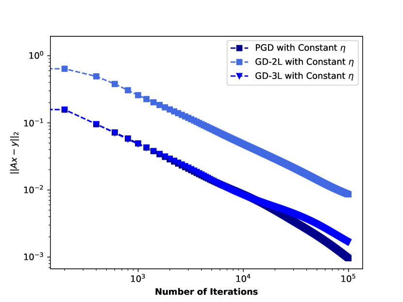
(a) With constant stepsize

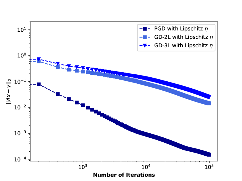
(b) With oracle stepsize

Figure 7: Comparison of convergence rate in the dense, non-sparse, case, cf. Section D.4.

References

- [1] Sanjeev Arora, Nadav Cohen, and Elad Hazan. On the optimization of deep networks: Implicit acceleration by overparameterization. In Proceedings of the 35th International Conference on Machine Learning, ICML 2018, pages 244–253, 2018.
- [2] Sanjeev Arora, Nadav Cohen, Wei Hu, and Yuping Luo. Implicit regularization in deep matrix factorization. In Advances in Neural Information Processing Systems, pages 7413–7424, 2019.
- [3] Hedy Attouch, Jérôme Bolte, and Benar Fux Svaiter. Convergence of descent methods for semi-algebraic and tame problems: proximal algorithms, forward–backward splitting, and regularized gauss–seidel methods. Mathematical Programming, 137(1):91–129, 2013.
- [4] Jonathan Barzilai and Jonathan M Borwein. Two-point step size gradient methods. IMA journal of numerical analysis, 8(1):141–148, 1988.
- [5] Stefania Bellavia, Maria Macconi, and Benedetta Morini. An interior point Newton-like method for non-negative least-squares problems with degenerate solution. Numerical Linear Algebra with Applications, 13(10):825–846, 2006.
- [6] Federico Benvenuto, Riccardo Zanella, Luca Zanni, and Mario Bertero. Nonnegative least-squares image deblurring: improved gradient projection approaches. Inverse Problems, 26(2):025004, 2009.
- [7] Aaron Berk, Yaniv Plan, and Ozgur Yilmaz. On the best choice of LASSO program given data parameters. IEEE Transactions on Information Theory, 2021.
- [8] Michel Bierlaire, Ph L Toint, and Daniel Tuyttens. On iterative algorithms for linear least squares problems with bound constraints. Linear Algebra and its Applications, 143:111–143, 1991.
- [9] Ake Björck. Numerical Methods for Least Squares Problems. Society for Industrial and Applied Mathematics, 1996.
- [10] L.M. Bregman. The relaxation method of finding the common point of convex sets and its application to the solution of problems in convex programming. USSR Computational Mathematics and Mathematical Physics, 7(3):200–217, 1967.
- [11] Rasmus Bro and Sijmen De Jong. A fast non-negativity-constrained least squares algorithm. Journal of Chemometrics: A Journal of the Chemometrics Society, 11(5):393–401, 1997.
- [12] Alfred M Bruckstein, Michael Elad, and Michael Zibulevsky. On the uniqueness of nonnegative sparse solutions to underdetermined systems of equations. IEEE Transactions on Information Theory, 54(11):4813–4820, 2008.
- [13] Sébastien Bubeck et al. Convex optimization: Algorithms and complexity. Foundations and Trends® in Machine Learning, 8(3-4):231–357, 2015.
- [14] Emmanuel J. Candès, Justin K. Romberg, and Terence Tao. Stable signal recovery from incomplete and inaccurate measurements. Comm. Pure Appl. Math., 59(8):1207–1223, 2006.
- [15] Emmanuel J. Candès and Terence Tao. Near-Optimal Signal Recovery From Random Projections: Universal Encoding Strategies? IEEE Transactions on Information Theory, 52(12):5406–5425, 2006.
- [16] Donghui Chen and Robert J Plemmons. Nonnegativity constraints in numerical analysis. In The birth of numerical analysis, pages 109–139. World Scientific, 2010.
- [17] Jie Chen, Cédric Richard, José Carlos M Bermudez, and Paul Honeine. Nonnegative least-mean-square algorithm. IEEE Transactions on Signal Processing, 59(11):5225–5235, 2011.
- [18] Scott Shaobing Chen, David L Donoho, and Michael A Saunders. Atomic decomposition by basis pursuit. SIAM Rev., 43(1):129–159, 2001.
- [19] Shaobing Scott Chen and David L Donoho. Basis pursuit. In Proc. of 1994 28th Asilomar Conference on Signals, Systems and Computers, pages 41–44, 1994.
- [20] Hung-Hsu Chou, Carsten Gieshoff, Johannes Maly, and Holger Rauhut. Gradient descent for deep matrix factorization: Dynamics and implicit bias towards low rank. arXiv preprint: 2011.13772, 2020.
- [21] Hung-Hsu Chou, Johannes Maly, and Holger Rauhut. More is Less: Inducing Sparsity via Overparameterization. arXiv preprint arXiv:2112.11027, 2021.
- [22] Delin Chu, Weya Shi, Srinivas Eswar, and Haesun Park. An alternating rank-k nonnegative least squares framework (ARkNLS) for nonnegative matrix factorization. SIAM Journal on Matrix Analysis and Applications, 42(4):1451–1479, 2021.
- [23] Yu-Hong Dai and Roger Fletcher. Projected Barzilai-Borwein methods for large-scale box-constrained quadratic programming. Numerische Mathematik, 100(1):21–47, 2005.
- [24] Monica Dessole, Marco Dell’Orto, and Fabio Marcuzzi. The Lawson-Hanson Algorithm with Deviation Maximization: Finite Convergence and Sparse Recovery. arXiv preprint arXiv:2108.05345, 2021.
- [25] David L Donoho. Compressed sensing. IEEE Transactions on Information Theory, 52(4):1289–1306, 2006.
- [26] David L Donoho, Iain M Johnstone, Jeffrey C Hoch, and Alan S Stern. Maximum entropy and the nearly black object. Journal of the Royal Statistical Society: Series B (Methodological), 54(1):41–67, 1992.
- [27] David L Donoho and Jared Tanner. Sparse nonnegative solution of underdetermined linear equations by linear programming. Proceedings of the National Academy of Sciences, 102(27):9446–9451, 2005.
- [28] David L Donoho and Jared Tanner. Counting the faces of randomly-projected hypercubes and orthants, with applications. Discrete & Computational Geometry, 43(3):522–541, 2010.
- [29] Ernie Esser, Yifei Lou, and Jack Xin. A method for finding structured sparse solutions to nonnegative least squares problems with applications. SIAM Journal on Imaging Sciences, 6(4):2010–2046, 2013.
- [30] Roger Fletcher. On the Barzilai-Borwein method. In Optimization and control with applications, pages 235–256. Springer, 2005.
- [31] Simon Foucart and Holger Rauhut. A Mathematical Introduction to Compressive Sensing. Birkhäuser, New York, NY, 2013.
- [32] Kelly Geyer, Anastasios Kyrillidis, and Amir Kalev. Low-rank regularization and solution uniqueness in over-parameterized matrix sensing. In Proceedings of the 23rd International Conference on Artificial Intelligence and Statistics, pages 930–940, 2020.
- [33] Gauthier Gidel, Francis Bach, and Simon Lacoste-Julien. Implicit regularization of discrete gradient dynamics in linear neural networks. In Advances in Neural Information Processing Systems, pages 3202–3211, 2019.
- [34] Philip E Gill and Walter Murray. A numerically stable form of the simplex algorithm. Linear algebra and its applications, 7(2):99–138, 1973.
- [35] Daniel Gissin, Shai Shalev-Shwartz, and Amit Daniely. The implicit bias of depth: How incremental learning drives generalization. International Conference on Learning Representations (ICLR)., 2020.
- [36] Gene H. Golub and Michael A. Saunders. Linear least squares and quadratic programming. In Jean Abadie and Philip Wolfe, editors, Integer and Nonlinear Programming, pages 229–256. North Holland Pub. Co., Amsterdam, 1970.
- [37] Ian Goodfellow, Jean Pouget-Abadie, Mehdi Mirza, Bing Xu, David Warde-Farley, Sherjil Ozair, Aaron Courville, and Yoshua Bengio. Generative adversarial nets. In Z. Ghahramani, M. Welling, C. Cortes, N. Lawrence, and K.Q. Weinberger, editors, Advances in Neural Information Processing Systems, volume 27. Curran Associates, Inc., 2014.
- [38] Suriya Gunasekar, Jason D Lee, Daniel Soudry, and Nati Srebro. Implicit bias of gradient descent on linear convolutional networks. In Advances in Neural Information Processing Systems, pages 9461–9471, 2018.
- [39] Suriya Gunasekar, Blake E Woodworth, Srinadh Bhojanapalli, Behnam Neyshabur, and Nati Srebro. Implicit regularization in matrix factorization. In Advances in Neural Information Processing Systems, pages 6151–6159, 2017.
- [40] Sepp Hochreiter and Jürgen Schmidhuber. Flat minima. Neural computation, 9(1):1–42, 1997.
- [41] Peter D Hoff. Lasso, fractional norm and structured sparse estimation using a Hadamard product parametrization. Computational Statistics & Data Analysis, 115:186–198, 2017.
- [42] Arthur Jacot, Franck Gabriel, and Clément Hongler. Neural tangent kernel: Convergence and generalization in neural networks. Advances in Neural Information Processing Systems, 31, 2018.
- [43] Jun Beom Kho, Jaihie Kim, Ig-Jae Kim, and Andrew BJ Teoh. Cancelable fingerprint template design with randomized non-negative least squares. Pattern Recognition, 91:245–260, 2019.
- [44] Dongmin Kim, Suvrit Sra, and Inderjit S Dhillon. A non-monotonic method for large-scale non-negative least squares. Optimization Methods and Software, 28(5):1012–1039, 2013.
- [45] Hyunsoo Kim, Yingtao Bi, Sharmistha Pal, Ravi Gupta, and Ramana V Davuluri. IsoformEx: isoform level gene expression estimation using weighted non-negative least squares from mRNA-Seq data. BMC bioinformatics, 12(1):1–9, 2011.
- [46] Richard Kueng and Peter Jung. Robust nonnegative sparse recovery and the nullspace property of 0/1 measurements. IEEE Transactions on Information Theory, 64(2):689–703, 2017.
- [47] Charles L Lawson and Richard J Hanson. Solving least squares problems. SIAM, 1995.
- [48] Jiangyuan Li, Thanh Nguyen, Chinmay Hegde, and Ka Wai Wong. Implicit sparse regularization: The impact of depth and early stopping. In Advances in Neural Information Processing Systems, 2021.
- [49] Chih-Jen Lin. Projected gradient methods for nonnegative matrix factorization. Neural computation, 19(10):2756–2779, 2007.
- [50] Sheng Liu, Zhihui Zhu, Qing Qu, and Chong You. Robust training under label noise by over-parameterization. In Kamalika Chaudhuri, Stefanie Jegelka, Le Song, Csaba Szepesvari, Gang Niu, and Sivan Sabato, editors, Proceedings of the 39th International Conference on Machine Learning, volume 162 of Proceedings of Machine Learning Research, pages 14153–14172. PMLR, 17–23 Jul 2022.
- [51] Yuancheng Luo and Ramani Duraiswami. Efficient parallel nonnegative least squares on multicore architectures. SIAM Journal on Scientific Computing, 33(5):2848–2863, 2011.
- [52] Nicolai Meinshausen. Sign-constrained least squares estimation for high-dimensional regression. Electronic Journal of Statistics, 7:1607–1631, 2013.
- [53] Joe M Myre, Erich Frahm, David J Lilja, and Martin O Saar. TNT-NN: a fast active set method for solving large non-negative least squares problems. Procedia Computer Science, 108:755–764, 2017.
- [54] Joseph M Myre, Ioan Lascu, Eduardo A Lima, Joshua M Feinberg, Martin O Saar, and Benjamin P Weiss. Using TNT-NN to unlock the fast full spatial inversion of large magnetic microscopy data sets. Earth, Planets and Space, 71(1):1–26, 2019.
- [55] Yurii E Nesterov. A method for solving the convex programming problem with convergence rate O(1/k^2 ). In Dokl. akad. nauk SSSR, volume 269, pages 543–547, 1983.
- [56] Behnam Neyshabur, Ryota Tomioka, Ruslan Salakhutdinov, and Nathan Srebro. Geometry of optimization and implicit regularization in deep learning. arXiv preprint arXiv:1705.03071, 2017.
- [57] Behnam Neyshabur, Ryota Tomioka, and Nathan Srebro. In search of the real inductive bias: On the role of implicit regularization in deep learning. In International Conference on Learning Representations, 2015.
- [58] Ji Peng, Jerrad Hampton, and Alireza Doostan. A weighted -minimization approach for sparse polynomial chaos expansions. Journal of Computational Physics, 267:92–111, 2014.
- [59] Scott Pesme, Loucas Pillaud-Vivien, and Nicolas Flammarion. Implicit Bias of SGD for Diagonal Linear Networks: a Provable Benefit of Stochasticity. Advances in Neural Information Processing Systems, 34, 2021.
- [60] Roman A Polyak. Projected gradient method for non-negative least square. Contemp Math, 636:167–179, 2015.
- [61] Holger Rauhut and Rachel Ward. Interpolation via weighted -minimization. Applied and Computational Harmonic Analysis, 40(2):321–351, 2016.
- [62] Marcos Raydan. The Barzilai and Borwein gradient method for the large scale unconstrained minimization problem. SIAM Journal on Optimization, 7(1):26–33, 1997.
- [63] Noam Razin and Nadav Cohen. Implicit regularization in deep learning may not be explainable by norms. In Advances in Neural Information Processing Systems, pages 21174–21187, 2020.
- [64] Yonatan Shadmi, Peter Jung, and Giuseppe Caire. Sparse non-negative recovery from biased subgaussian measurements using NNLS. arXiv preprint arXiv:1901.05727, 2019.
- [65] Martin Slawski and Matthias Hein. Sparse recovery by thresholded non-negative least squares. Advances in Neural Information Processing Systems, 24, 2011.
- [66] Martin Slawski and Matthias Hein. Non-negative least squares for high-dimensional linear models: Consistency and sparse recovery without regularization. Electronic Journal of Statistics, 7:3004–3056, 2013.
- [67] Daniel Soudry, Elad Hoffer, Mor Shpigel Nacson, Suriya Gunasekar, and Nathan Srebro. The implicit bias of gradient descent on separable data. The Journal of Machine Learning Research, 19(1):2822–2878, 2018.
- [68] Grzegorz Stoch and Artur T Krzyżak. Enhanced Resolution Analysis for Water Molecules in MCM-41 and SBA-15 in Low-Field T2 Relaxometric Spectra. Molecules, 26(8):2133, 2021.
- [69] Josef Stoer. On the numerical solution of constrained least-squares problems. SIAM journal on Numerical Analysis, 8(2):382–411, 1971.
- [70] Dominik Stöger and Mahdi Soltanolkotabi. Small random initialization is akin to spectral learning: Optimization and generalization guarantees for overparameterized low-rank matrix reconstruction. Advances in Neural Information Processing Systems, 34, 2021.
- [71] Robert Tibshirani. Regression shrinkage and selection via the lasso. Journal of the Royal Statistical Society: Series B (Methodological), 58(1):267–288, 1996.
- [72] Mark H Van Benthem and Michael R Keenan. Fast algorithm for the solution of large-scale non-negativity-constrained least squares problems. Journal of Chemometrics: A Journal of the Chemometrics Society, 18(10):441–450, 2004.
- [73] Vladimir Vapnik. The nature of statistical learning theory. Springer science & business media, 1999.
- [74] Tomas Vaskevicius, Varun Kanade, and Patrick Rebeschini. Implicit regularization for optimal sparse recovery. In Advances in Neural Information Processing Systems, pages 2972–2983, 2019.
- [75] Meng Wang, Weiyu Xu, and Ao Tang. A unique “nonnegative” solution to an underdetermined system: From vectors to matrices. IEEE Transactions on Signal Processing, 59(3):1007–1016, 2010.
- [76] Yuqing Wang, Minshuo Chen, Tuo Zhao, and Molei Tao. Large Learning Rate Tames Homogeneity: Convergence and Balancing Effect. In International Conference on Learning Representations, 2022.
- [77] Blake Woodworth, Suriya Gunasekar, Jason D. Lee, Edward Moroshko, Pedro Savarese, Itay Golan, Daniel Soudry, and Nathan Srebro. Kernel and Rich Regimes in Overparametrized Models. In Proceedings of Thirty Third Conference on Learning Theory, pages 3635–3673, 2020.
- [78] Fan Wu and Patrick Rebeschini. Implicit Regularization in Matrix Sensing via Mirror Descent. Advances in Neural Information Processing Systems, 34, 2021.
- [79] Chong You, Zhihui Zhu, Qing Qu, and Yi Ma. Robust recovery via implicit bias of discrepant learning rates for double over-parameterization. In H. Larochelle, M. Ranzato, R. Hadsell, M.F. Balcan, and H. Lin, editors, Advances in Neural Information Processing Systems, volume 33, pages 17733–17744. Curran Associates, Inc., 2020.
- [80] Chiyuan Zhang, Samy Bengio, Moritz Hardt, Benjamin Recht, and Oriol Vinyals. Understanding deep learning requires rethinking generalization. In International Conference on Learning Representations, 2017.
- [81] Chiyuan Zhang, Samy Bengio, Moritz Hardt, Benjamin Recht, and Oriol Vinyals. Understanding deep learning (still) requires rethinking generalization. Communications of the ACM, 64(3):107–115, 2021.
- [82] Peng Zhao, Yun Yang, and Qiao-Chu He. Implicit Regularization via Hadamard Product Over-Parametrization in High-Dimensional Linear Regression. arXiv preprint: 1903.09367, 2019.