Discontinuous Galerkin Approximations to Elliptic and Parabolic Problems with a Dirac Line Source

Abstract.

The analyses of interior penalty discontinuous Galerkin methods of any order $k$ for solving elliptic and parabolic problems with Dirac line sources are presented. For the steady state case, we prove convergence of the method by deriving a priori error estimates in the $L^{2}$ norm and in weighted energy norms. In addition, we prove almost optimal local error estimates in the energy norm for any approximation order. Further, almost optimal local error estimates in the $L^{2}$ norm are obtained for the case of piecewise linear approximations whereas suboptimal error bounds in the $L^{2}$ norm are shown for any polynomial degree. For the time-dependent case, convergence of semi-discrete and of backward Euler fully discrete scheme is established by proving error estimates in $L^{2}$ in time and in space. Numerical results for the elliptic problem are added to support the theoretical results.

1. Introduction

In this paper, we analyze interior penalty discontinuous Galerkin (dG) approximations to elliptic and parabolic problems with a Dirac measure concentrated on a line. Consider a convex domain $\Omega\subset\mathbbm{R}^{3}$ containing a one-dimensional curve $\Lambda\subset\mathbbm{R}$ which is strictly included in $\Omega$. The elliptic model problem reads

(1.1) $$-\Delta u =f\delta_{\Lambda}, \quad\text{in }\Omega,$$

(1.2) $$u =0, \quad\text{on }\partial\Omega.$$

where $f\in L^{2}(\Lambda)$ and $f\delta_{\Lambda}$ is a Dirac measure concentrated on $\Lambda$ defined as follows.

(1.3) $$\langle f\delta_{\Lambda},v\rangle=\int_{\Lambda}fvds,\quad\forall v\in L^{\infty}(\Omega).$$

For the parabolic problem, let $T$ be the final time, let $u^{0}$ be in $L^{2}(\Omega)$ and assume that $f$ belongs to $L^{2}(0,T;L^{2}(\Lambda))$. We consider the following problem.

(1.4) $$\partial_{t}u-\Delta u =f\delta_{\Lambda}, \quad\mathrm{in}\,\,\Omega\times(0,T],$$

(1.5) $$u =0, \quad\mathrm{on}\,\,\partial\Omega\times(0,T],$$

(1.6) $$u =u^{0}, \quad\mathrm{in}\,\,\{0\}\times\Omega.$$

The main contributions of this work are as follows. For the elliptic problem, we show global convergence in the $L^{2}$ norm and in weighted energy norms. Further, in regions excluding the line $\Lambda$, we derive almost optimal $L^{2}$ error estimates for linear polynomials and suboptimal error bounds of order almost $k$ for dG approximations of degree $k\geq 2$. In addition, almost optimal error rates are established in local energy norms for approximations of any polynomial degree. For the parabolic problem, we show global convergence in the $L^{2}(0,T;L^{2}(\Omega))$ norm for both the semi-discrete approximation and for the backward Euler fully discrete scheme.

Partial differential equations with Dirac right-hand sides can model organ perfusion where blood vessels are considered as one dimensional fractures embedded in the tissue [13]. In this case, $f$ can be a function of the blood pressure in the vessel leading to a coupled 1D-3D problem for the pressures in the tissue and in the vessels [12, 13]. Medical applications of such formulations include modeling drug delivery to tissues with the help of implantable devices [11] and drug delivery to tumors where different treatment options are compared [6]. In addition, Dirac measures concentrated on lines arise in optimal control problems [23]. Thanks to favorable properties of dG methods, including local mass conservation and adaptability to complex domains [32], these methods are well suited to model physical phenomena such as organ perfusion. In this paper we study dG methods applied to (1.1)-(1.2) and to (1.4)-(1.6).

The analysis of finite element approximations to model problems (1.1)-(1.2) and (1.4)-(1.6) is non–standard since the true solution is not smooth enough in space, namely it does not belong to $H^{1}(\Omega)$ and it exhibits a logarithmic singularity near the line $\Lambda$ [12, 26, 2]. Nevertheless, continuous Galerkin (cG) approximations have been extensively studied; we refer to the work by Scott [33] and Casas [5] where global error bounds are established. More recently and in the context of optimal control problems, Gong et al. derived improved global $L^{2}$ error bounds [23]. Such bounds are polluted by the singularity of the true solution where the rate of convergence in the $L^{2}$ norm for any polynomial degree is at most $\mathcal{O}(h)$ where $h$ is the mesh-size. For continuous Galerkin approximations to (1.4)-(1.6), global error estimates for semi-discrete and fully-discrete formulations are derived in [24, 22].

In addition, convergence of the cG approximations to the elliptic model problem (1.1)-(1.2) has been investigated in different non–classical norms. For example, local $L^{2}$ optimal error estimates (up to a log factor for linear polynomials) are derived by Köppl et al. [27, 26], and local energy error estimates are obtained by Bertoluzza et al. [3]. Such improved estimates are possible since the solution is smooth in regions excluding the line $\Lambda$ [2]. In addition, D’Angelo obtained error estimates in weighted norms and showed that with graded meshes the finite element solution converges optimally in these norms [12]. We also mention the recent splitting technique to numerically approximate the model problem (1.1)-(1.2) introduced by Gjerde et al. where the solution is split into an explicit singular part and an implicit smooth part [20]. A finite element discretization is then formulated for the smooth part and optimal error rates are recovered [20].

To the best of our knowledge, discontinuous Galerkin approximations to (1.1)-(1.2) and to (1.4)-(1.6) are missing from the literature. However, there are papers which formulate and study dG methods for elliptic problems with Dirac sources concentrated at a point. To this end, we mention the work by Houston and Wihler where global a priori and a posteriori error bounds are derived [25]. Recently, Choi and Lee derived local $L^{2}$ error estimates [8]. The analysis of dG methods for elliptic problems is particularly challenging since consistency of the numerical method cannot be assumed since the traces of the solution and its gradient are not well defined.

The rest of this paper is organized as follows. Weak formulations in usual and in weighted Sobolev spaces are presented and shown to be equivalent in Section 2. Then, Section 3 defines the cG and dG discrete solutions to model problem (1.1)-(1.2). We show global convergence in the $L^{2}$ norm in Section 4 and in weighted dG norms in Section 5. The local convergence of the solution is analyzed in Section 6. We devote Section 7 to the analysis of dG formulations for (1.4)-(1.6). Numerical results for the elliptic problem are presented in Section 8.

2. Weak formulation

Fix $p_{0}\in[1,3/2)$ and $q_{0}$ be such that $1/q_{0}+1/p_{0}=1$. Let $W^{1,p_{0}}(\Omega)$ denote the usual Sobolev space and recall that

$$W_{0}^{1,p_{0}}(\Omega)=\{v\in W^{1,p_{0}}(\Omega),\quad v=0\quad\mbox{on}\quad\partial\Omega\}.$$

The weak formulation for problem (1.1)-(1.2) is [5]: Find $u\in W_{0}^{1,p_{0}}(\Omega)$ such that:

(2.1) $$\int_{\Omega}\nabla u\cdot\nabla v=\int_{\Lambda}fv,\quad\forall v\in W_{0}^{1,q_{0}}(\Omega).$$

This weak formulation is well posed and a unique solution $u\in W_{0}^{1,p_{0}}(\Omega)$ for $p_{0}\in[1,3/2)$ exists [5]. Next, in a similar way to [12], we present another weak formulation of problem (1.1)-(1.2) in weighted Sobolev spaces. Define the distance function to $\Lambda$:

(2.2) $$d(\bm{x},\Lambda)=\text{dist}(\bm{x},\Lambda)=\min_{\bm{y}\in\Lambda}\|\bm{x}-\bm{y}\|,\quad\forall\bm{x}\in\Omega.$$

We first remark that $d^{\alpha}$ is an $A_{2}$ weight for $|\alpha|<2$ (see Lemma 3.3 in [17]) where $A_{2}$ is the Muckenhoupt class of weights satisfying:

$$A_{2}=\Big{\{}w\in L^{1}_{\mathrm{loc}}(\mathbbm{R}^{3}),\,\,\sup_{B(\bm{x},r)}\left(\frac{1}{|B(\bm{x},r)|}\int_{B(\bm{x},r)}w\right)\left(\frac{1}{|B(\bm{x},r)|}\int_{B(\bm{x},r)}w^{-1}\right)<\infty\Big{\}},$$

where the supremum is taken over all balls $B(\bm{x},r)$ centered at $\bm{x}$ and of radius $r$. This implies that $d^{\alpha}$ belongs to $L^{2}(\Omega)$ if $|\alpha|<1$. We assume that the distance function satisfies the following bounds (see Theorem 3.4 in [14]).

(2.3) $$\|\nabla d\|_{L^{\infty}(\Omega)}\leq 1,\quad\|\nabla^{2}d^{2}\|_{L^{\infty}(\Omega)}\leq C.$$

Using the fact the $\nabla d^{\alpha}=\alpha d^{\alpha-1}\nabla d$, we then have that $d^{\alpha}\in H^{1}(\Omega)$ if $0<\alpha<1$. For $\alpha\in(-1,1)$, define the weighted $L^{2}$ norm as follows.

(2.4) $$\|u\|_{L^{2}_{\alpha}(\Omega)}=\left(\int_{\Omega}|u|^{2}d^{2\alpha}\right)^{\frac{1}{2}}.$$

The $L^{2}_{\alpha}(\Omega)$ space and the weighted inner product are defined as:

$$L^{2}_{\alpha}(\Omega)=\{v:\,\|v\|_{L^{2}_{\alpha}(\Omega)}<\infty\},\quad(u,v)_{\alpha}=\int_{\Omega}uvd^{2\alpha},\quad\forall u,v\in L^{2}_{\alpha}(\Omega).$$

Similarly, we introduce the weighted Sobolev spaces as:

$$H^{m}_{\alpha}(\Omega)=\{u:D^{\bm{\beta}}u\in L^{2}_{\alpha}(\Omega),|\bm{\beta}|\leq m\},\,\,\,\mathring{H}^{m}_{\alpha}(\Omega)=\{u\in H^{m}_{\alpha}(\Omega),u|_{\partial\Omega}=0\}.$$

where $\bm{\beta}$ is a multi-index and $D^{\bm{\beta}}$ is the corresponding weak derivative. The weighted Sobolev semi-norms and norms are denoted by:

$$|u|_{H^{m}_{\alpha}(\Omega)}^{2}=\sum_{|\bm{\beta}|=m}\|D^{\bm{\beta}}u\|_{L^{2}_{\alpha}(\Omega)}^{2},\quad\|u\|_{H^{m}_{\alpha}(\Omega)}^{2}=\sum_{k=0}^{m}|u|_{H^{m}_{\alpha}(\Omega)}^{2}.$$

Lemma 1.

Let $\alpha$ be such that $-2/p_{0}+1<\alpha<2/p_{0}-1$. Then, the weak formulation (2.1) is equivalent to the following weak formulation: find $u_{\alpha}\in\mathring{H}^{1}_{\alpha}(\Omega)$ such that

(2.5) $$\int_{\Omega}\nabla u_{\alpha}\cdot\nabla v=\int_{\Lambda}fv,\quad\forall v\in\mathring{H}^{1}_{-\alpha}(\Omega).$$

Proof.

Let $u_{\alpha}$ be a solution of (2.5). The existence and uniqueness of $u_{\alpha}$ is established in [12], see also [16]. Observe that the condition on $\alpha$ implies that $(\alpha p_{0})/(2-p_{0})=(\alpha q_{0})/(q_{0}-2)\in(-1,1)$. Since $d^{\gamma}\in L^{1}_{\mathrm{loc}}(\mathbbm{R}^{3})$ for $|\gamma|\leq 2$, we use Hölder’s inequality and obtain

(2.6) $$\int_{\Omega}d^{-2\alpha}v^{2}\leq\left(\int_{\Omega}d^{-2\alpha\frac{q_{0}}{q_{0}-2}}\right)^{(q_{0}-2)/q_{0}}\|v\|^{2/q_{0}}_{L^{q_{0}}(\Omega)}<\infty,\quad\forall v\in L^{q_{0}}(\Omega).$$

This implies that $W_{0}^{1,q_{0}}(\Omega)\subset\mathring{H}^{1}_{-\alpha}(\Omega)$. Hence $u_{\alpha}$ satisfies (2.1) for all $v\in W_{0}^{1,q_{0}}(\Omega)$. Similarly, for $v\in L^{2}_{\alpha}(\Omega)$, we have

$$\int_{\Omega}v^{p_{0}}=\int_{\Omega}v^{p_{0}}d^{p_{0}\alpha}d^{-p_{0}\alpha}\leq\left(\int_{\Omega}v^{2}d^{2\alpha}\right)^{p_{0}/2}\left(\int_{\Omega}d^{-2\alpha\frac{p_{0}}{2-p_{0}}}\right)^{(2-p_{0})/2}<\infty,\quad\forall v\in L^{2}_{\alpha}(\Omega).$$

This implies that $\mathring{H}^{1}_{\alpha}(\Omega)\subset W_{0}^{1,p_{0}}(\Omega)$. Thus, $u_{\alpha}$ solves (2.1). Since the solution to (2.1) is unique (see Theorem 2.1 case (ii) in [23]), we conclude that $u_{\alpha}=u$. ∎

3. Numerical approximations

Let $\mathcal{E}_{h}$ denote a partition of $\Omega$, made of simplices:

(3.1) $$\bigcup_{E\in\mathcal{E}_{h}}\bar{E}=\bar{\Omega}.$$

The diameter of a given element $E$ is denoted by $h_{E}$ and the mesh size is denoted by $h=\max_{E\in\mathcal{E}_{h}}h_{E}$. We assume that $\mathcal{E}_{h}$ is regular in the sense that there exists a constant $\rho>0$ such that

(3.2) $$\frac{h_{E}}{\rho_{E}}\leq\rho,\quad\forall E\in\mathcal{E}_{h},$$

where $\rho_{E}$ is the maximum diameter of a ball inscribed in $E$. In addition, we assume that $\mathcal{E}_{h}$ is quasi-uniform: there is a constant $\gamma>0$ independent of $h$ such that

(3.3) $$h\leq\gamma h_{E},\quad\forall E\in\mathcal{E}_{h}.$$

The broken Sobolev space is denoted by $H^{m}(\mathcal{E}_{h})$ for $m\geq 1$, and the broken gradient is denoted by $\nabla_{h}$. In the remaining of the paper, $k\geq 1$ is a fixed positive integer and $C$ is a generic constant independent of $h$.

3.1. Finite element approximation

Let $W^{k}_{h}(\mathcal{E}_{h})$ be the finite element space defined as follows.

(3.4) $$W_{h}^{k}(\mathcal{E}_{h})=\{w_{h}\in H^{1}_{0}(\Omega):w_{h}|_{E}\in\mathbbm{P}^{k}(E),\,\,\forall E\in\mathcal{E}_{h}\}.$$

Here, $\mathbbm{P}^{k}(E)$ denotes the space of polynomials of degree at most $k$. Let $u_{h}^{\mathrm{CG}}\in W^{k}_{h}(\mathcal{E}_{h})$ be the finite element approximation to $u$ satisfying

(3.5) $$\int_{\Omega}\nabla u_{h}^{\mathrm{CG}}\cdot\nabla v_{h}=\int_{\Lambda}fv_{h},\quad\forall v_{h}\in W^{k}_{h}(\mathcal{E}_{h}).$$

3.2. Discontinuous Galerkin approximation

We now introduce the interior penalty discontinuous Galerkin discrete solution [32]. We define the broken polynomial space as follows.

(3.6) $$V_{h}^{k}(\mathcal{E}_{h})=\{v_{h}\in L^{2}(\Omega):v_{h}|_{E}\in\mathbbm{P}^{k}(E),\forall E\in\mathcal{E}_{h}\}.$$

We also denote by $\Gamma_{h}$ the set of all interior faces in $\mathcal{E}_{h}$. For each interior face $e$, we associate a unit normal vector $\bm{n}_{e}$ and we denote by $E_{e}^{1}$ and $E_{e}^{2}$ the two elements that share $e$ such that the vector $\bm{n}_{e}$ points from $E_{e}^{1}$ to $E_{e}^{2}$. We denote the average and the jump of a function $v_{h}\in V_{h}^{k}(\mathcal{E}_{h})$ by $\{v_{h}\}$ and $[v_{h}]$ respectively.

(3.7) $$\{v_{h}\}=\frac{1}{2}\left(v_{h}|_{E_{e}^{1}}+v_{h}|_{E_{e}^{2}}\right),\quad[v_{h}]=v_{h}|_{E_{e}^{1}}-v_{h}|_{E_{e}^{2}},\quad\forall e\in\Gamma_{h}.$$

If $e$ belongs to the boundary of the domain, $e=\partial\Omega\cap\partial E_{e}^{1}$, then we define the average and the jump as follows.

(3.8) $$[v]=\{v\}=v|_{E_{e}^{1}}.$$

Let $u_{h}^{\mathrm{DG}}\in V_{h}^{k}(\mathcal{E}_{h})$ be the discontinuous Galerkin solution satisfying:

(3.9) $$a_{\epsilon}(u_{h}^{\mathrm{DG}},v_{h})=\int_{\Lambda}fv_{h},\quad\forall v_{h}\in V_{h}^{k}(\mathcal{E}_{h}),$$

where $a_{\epsilon}(\cdot,\cdot):V_{h}^{k}(\mathcal{E}_{h})\times V_{h}^{k}(\mathcal{E}_{h})\rightarrow\mathbbm{R}$ is given by:

(3.10) $$a_{\epsilon}(u,v) = \sum_{E\in\mathcal{E}_{h}}\int_{E}\nabla u\cdot\nabla v-\sum_{e\in\Gamma_{h}\cup\partial\Omega}\int_{e}\{\nabla u\}\cdot\bm{n}_{e}[v]$$

$$+\epsilon\sum_{e\in\Gamma_{h}\cup\partial\Omega}\int_{e}\{\nabla v\}\cdot\bm{n}_{e}[u]+\sum_{e\in\Gamma_{h}\cup\partial\Omega}\int_{e}\frac{\sigma}{h^{\beta}}[u][v].$$

In the above, $\epsilon\in\{-1,0,1\}$, $\sigma$ is a user specified parameter and $\beta\geq 1$ is a parameter to be specified in the subsequent sections. We define the following energy semi-norm. For $B\subseteq\Omega$ or $B=\overline{\Omega}$ and $v_{h}\in V_{h}^{k}(\mathcal{E}_{h})$,

(3.11) $$\|v_{h}\|^{2}_{\mathrm{DG}(B)}=\sum_{E\in\mathcal{E}_{h}}\|\nabla v_{h}\|^{2}_{L^{2}(E\cap B)}+\sum_{e\in\Gamma_{h}\cup\partial\Omega}\sigma h^{-1}\|[v_{h}]\|^{2}_{L^{2}(e\cap B)}.$$

For simplicity, we write $\|\cdot\|^{2}_{\mathrm{DG}}=\|\cdot\|^{2}_{\mathrm{DG}(\overline{\Omega})}$. We also note that $\|\cdot\|_{\mathrm{DG}}$ defines a norm and the following Poincare inequality holds [15].

(3.12) $$\|v_{h}\|_{L^{p}(\Omega)}\leq C\|v_{h}\|_{\mathrm{DG}},\quad\forall 1\leq p\leq 6,\,\,\,\forall v_{h}\in V_{h}^{k}(\mathcal{E}_{h}).$$

In the analysis, we will also use the following semi-norm. For $v\in H^{2}(\mathcal{E}_{h})$ and $B\subseteq\Omega$ or $B=\overline{\Omega}$,

(3.13) $${\left|\kern-1.07639pt\left|\kern-1.07639pt\left|v\right|\kern-1.07639pt\right|\kern-1.07639pt\right|}^{2}_{\mathrm{DG}(B)}=\|v\|^{2}_{\mathrm{DG}(B)}+\sum_{e\in\Gamma_{h}\cup\partial\Omega}h\|\{\nabla v\}\|^{2}_{L^{2}(e\cap B)}.$$

Similarly, denote ${\left|\kern-1.07639pt\left|\kern-1.07639pt\left|\cdot\right|\kern-1.07639pt\right|\kern-1.07639pt\right|}_{\mathrm{DG}}^{2}={\left|\kern-1.07639pt\left|\kern-1.07639pt\left|\cdot\right|\kern-1.07639pt\right|\kern-1.07639pt\right|}_{\mathrm{DG}(\overline{\Omega})}^{2}$. We then have the following continuity properties of the form $a_{\epsilon}$ [7, 32].

(3.14) $$a_{\epsilon}(v,w)\leq C{\left|\kern-1.07639pt\left|\kern-1.07639pt\left|v\right|\kern-1.07639pt\right|\kern-1.07639pt\right|}_{\mathrm{DG}}{\left|\kern-1.07639pt\left|\kern-1.07639pt\left|w\right|\kern-1.07639pt\right|\kern-1.07639pt\right|}_{\mathrm{DG}},\quad a_{\epsilon}(v_{h},w_{h})\leq C\|v_{h}\|_{\mathrm{DG}}\|w_{h}\|_{\mathrm{DG}},\quad\forall v,w\in H^{2}(\mathcal{E}_{h}),\,\forall v_{h},w_{h}\in V_{h}^{k}(\mathcal{E}_{h}).$$

In addition, the following coercivity property

(3.15) $$a_{\epsilon}(w_{h},w_{h})\geq\frac{1}{2}\|w_{h}\|^{2}_{\mathrm{DG}},\quad\forall w_{h}\in V_{h}^{k}(\mathcal{E}_{h}),$$

is valid for any value $\sigma\geq 1$ if $\epsilon=+1$ and for $\sigma$ large enough if $\epsilon=-1,0$. We recall the following important inverse inequalities, see Section 4.5 in [4].

(3.16) $$\|v_{h}\|_{L^{q}(\Omega)}\leq Ch^{\frac{3}{q}-\frac{3}{p}}\|v_{h}\|_{L^{p}(\Omega)},\quad\forall\,1\leq p\leq q\leq\infty,\,\,\,\forall\,v_{h}\in V_{h}^{k}(\mathcal{E}_{h}).$$

For the trace estimates, we will make use of the following.

(3.17) $$\|v\|_{L^{2}(e)}\leq Ch^{-1/2}(\|v\|_{L^{2}(E)}+h\|\nabla v\|_{L^{2}(E)}),\quad\forall e\subset\partial E,\quad\forall E\in\mathcal{E}_{h},\quad\forall v\in H^{1}(\mathcal{E}_{h}).$$

For discrete functions, the above estimate reads

(3.18) $$\|v_{h}\|_{L^{2}(e)}\leq Ch^{-1/2}\|v_{h}\|_{L^{2}(E)},\quad\forall e\subset\partial E,\quad\forall E\in\mathcal{E}_{h},\quad\forall v_{h}\in V_{h}^{k}(\mathcal{E}_{h}).$$

Further, we recall that for any $p\in[1,\infty]$,

(3.19) $$\|\nabla_{h}v_{h}\|_{L^{p}(\Omega)}\leq Ch^{-1}\|v_{h}\|_{L^{p}(\Omega)},\quad\forall v_{h}\in V_{h}^{k}(\mathcal{E}_{h}).$$

4. Global error estimate in the $L^{2}$ norm

The goal of this section is to show a global $L^{2}$ estimate for the error $u$ - $u^{\mathrm{DG}}_{h}$. We first recall important global $L^{2}$ estimates for the finite element discretization (3.5). For $k=1$. Casas obtained the following estimate [5],

(4.1) $$\|u-u_{h}^{\mathrm{CG}}\|_{L^{2}(\Omega)}\leq Ch^{1/2}\|f\|_{L^{2}(\Lambda)}.$$

If the line $\Lambda$ is a $\mathcal{C}^{2}$ curve that does not intersect the boundary $\partial\Omega$, the improved estimate

(4.2) $$\|u-u_{h}^{\mathrm{CG}}\|_{L^{2}(\Omega)}\leq C(\theta)h^{1-\theta}\|f\|_{L^{2}(\Lambda)},\quad 0<\theta<\frac{1}{2},$$

was proved by Gong et al. for $k=1$ in [23]. Similar arguments yield the same error bounds for $k\geq 2$. The parameter $\theta$ arises from the fact that $u\in W_{0}^{1,\frac{6}{2\theta+3}}(\Omega)$ when $0<\theta<1/2$. We follow the ideas of Scott [33] and Houston and Wihler [25] presented for a problem with a Dirac source concentrated at a point, and we construct an intermediate problem with an $L^{2}$ source term. Let $\mathcal{T}_{\Lambda}\subset\mathcal{E}_{h}$ be the set of elements that intersect the line $\Lambda$,

$$\mathcal{T}_{\Lambda}=\{E\in\mathcal{E}_{h},\,\,\,E\cap\Lambda\neq\emptyset\}.$$

Define $f_{h}\in V_{h}^{k}(\mathcal{E}_{h})$ as

(4.3) $$\forall E\in\mathcal{E}_{h},\quad f_{h}|_{E}=\begin{cases}f_{h,E},&\mbox{if }\,E\in\mathcal{T}_{\Lambda},\\ 0,&\text{otherwise},\end{cases}$$

where $f_{h,E}\in\mathbbm{P}^{k}(E)$ is defined as follows. For $E\in\mathcal{T}_{\Lambda}$,

(4.4) $$\int_{E}f_{h,E}v_{h}=\int_{E\cap\Lambda}fv_{h},\quad\forall v_{h}\in\mathbbm{P}^{k}(E).$$

Clearly, the function $f_{h,E}$ is well defined. Further, consider the following intermediate problem: find $U\in H_{0}^{1}(\Omega)$ such that

(4.5) $$-\Delta U =f_{h}, \quad\text{in}\,\,\Omega,$$

(4.6) $$U =0, \quad\text{on}\,\,\partial\Omega.$$

Since $f_{h}$ belongs to $L^{2}(\Omega)$, Lax-Milgram’s theorem yields existence and uniqueness of $U$. In addition, since $\Omega$ is convex, the function $U$ belongs to $H^{2}(\Omega)$. We proceed by obtaining a bound on $f_{h}$ in the following lemma.

Lemma 2.

The following estimate holds

(4.7) $$\|f_{h}\|_{L^{2}(\Omega)}\leq Ch^{-3/2}\|f\|_{L^{2}(\Lambda)}.$$

In addition, if $\Lambda$ is a $\mathcal{C}^{2}$ curve and the mesh satisfies $|\Lambda\cap E|\leq Ch$ for all $E\in\mathcal{E}_{h}$, we have

(4.8) $$\|f_{h}\|_{L^{2}(\Omega)}\leq Ch^{-1}\|f\|_{L^{2}(\Lambda)}.$$

Proof.

With the definition of $f_{h}$ given in (4.4), we have

$$\|f_{h}\|^{2}_{L^{2}(\Omega)}=\int_{\Omega}f_{h}^{2} =\sum_{E\in\mathcal{E}_{h}}\int_{E}(f_{h}|_{E})^{2}=\sum_{E\in\mathcal{T}_{\Lambda}}\int_{E\cap\Lambda}f_{h,E}f.$$

Using Hölder’s inequality, we obtain

$$\int_{E\cap\Lambda}f_{h,E}f\leq\|f_{h,E}\|_{L^{\infty}(E)}\|f\|_{L^{1}(E\cap\Lambda)}.$$

Hence, with (3.16) ($q=\infty,p=2$), and (3.3), we obtain

$$\|f_{h}\|^{2}_{L^{2}(\Omega)}\leq\sum_{E\in\mathcal{T}_{\Lambda}}\|f_{h,E}\|_{L^{\infty}(E)}\|f\|_{L^{1}(E\cap\Lambda)} \leq Ch^{-3/2}\sum_{E\in\mathcal{T}_{\Lambda}}\|f_{h,E}\|_{L^{2}(E)}\|f\|_{L^{1}(E\cap\Lambda)}$$

$$\leq Ch^{-3/2}\sum_{E\in\mathcal{T}_{\Lambda}}\|f_{h,E}\|_{L^{2}(E)}|\Lambda\cap E|^{1/2}\|f\|_{L^{2}(E\cap\Lambda)}.$$

If $|\Lambda\cap E|\leq Ch$, we apply Hölder’s inequality for sums and obtain (4.8). Otherwise, we have (4.7). ∎

The following a priori error bounds hold.

Lemma 3.

There exists a constant $C$ independent of $h$ such that

(4.9) $$\|U-u_{h}^{\mathrm{CG}}\|_{L^{2}(\Omega)}+h\|\nabla(U-u_{h}^{\mathrm{CG}})\|_{L^{2}(\Omega)}\leq Ch^{2}\|U\|_{H^{2}(\Omega)},$$

(4.10) $${\left|\kern-1.07639pt\left|\kern-1.07639pt\left|U-u_{h}^{\mathrm{DG}}\right|\kern-1.07639pt\right|\kern-1.07639pt\right|}_{\mathrm{DG}}\leq Ch\|U\|_{H^{2}(\Omega)}.$$

If in addition, $\beta=1$ and $\sigma$ is large enough if $\epsilon=-1$ or $\beta>3/2$ and $\sigma$ is large enough for $\epsilon=0$ or $\epsilon=1$, there exists a constant $C$ independent of $h$ such that

(4.11) $$\|U-u_{h}^{\mathrm{DG}}\|_{L^{2}(\Omega)}\leq Ch^{2}\|U\|_{H^{2}(\Omega)}.$$

Proof.

We have for any $v_{h}\in V_{h}^{k}(\mathcal{E}_{h})$,

$$\int_{\Omega}f_{h}v_{h}=\sum_{E\in\mathcal{E}_{h}}\int_{E}f_{h}|_{E}\,v_{h}=\sum_{E\in\mathcal{T}_{\Lambda}}\int_{E\cap\Lambda}fv_{h}=\int_{\Lambda}fv_{h}.$$

Thus, since $W_{h}^{k}(\mathcal{E}_{h})$ is a subset of $V_{h}^{k}(\mathcal{E}_{h}$), the discrete functions $u_{h}^{\mathrm{CG}}$ and $u^{\mathrm{DG}}_{h}$ can be viewed as finite element and discontinuous Galerkin approximations to the intermediate problem (4.5). Since $f_{h}\in L^{2}(\Omega)$, standard approximation and error bounds hold. In particular, (4.9) and (4.10) hold. For a proof of (4.11), we refer to Theorem 2.13 in [32]. ∎

We are now ready to present and prove the main result of this section.

Theorem 1.

Assume the penalty parameter $\sigma$ is chosen so that (3.15) holds. In addition, if $\epsilon=\{0,1\}$, select $\beta>3/2$ and if $\epsilon=-1$, choose $\beta=1$. Then, there exists a constant $C$ independent of $h$ such that

(4.12) $$\|u-u^{\mathrm{DG}}_{h}\|_{L^{2}(\Omega)}\leq Ch^{1/2}\|f\|_{L^{2}(\Lambda)}.$$

In addition, if $\Lambda$ is a $\mathcal{C}^{2}$ curve and $|\Lambda\cap\overline{E}|\leq Ch$ for all $E\in\mathcal{E}_{h}$, we have the following improved estimate.

(4.13) $$\|u-u^{\mathrm{DG}}_{h}\|_{L^{2}(\Omega)}\leq C(\theta)h^{1-\theta}\|f\|_{L^{2}(\Lambda)},\quad 0<\theta<1/2.$$

Proof.

We use triangle inequality to obtain:

(4.14) $$\|u-u^{\mathrm{DG}}_{h}\|_{L^{2}(\Omega)}\leq\|u-u_{h}^{\mathrm{CG}}\|_{L^{2}(\Omega)}+\|u_{h}^{\mathrm{CG}}-U\|_{L^{2}(\Omega)}+\|U-u^{\mathrm{DG}}_{h}\|_{L^{2}(\Omega)}.$$

We have for any $v_{h}\in V_{h}^{k}(\mathcal{E}_{h})$,

$$\int_{\Omega}f_{h}v_{h}=\sum_{E\in\mathcal{E}_{h}}\int_{E}f_{h}|_{E}\,v_{h}=\sum_{E\in\mathcal{T}_{\Lambda}}\int_{E\cap\Lambda}fv_{h}=\int_{\Lambda}fv_{h}.$$

Since the domain $\Omega$ is convex, we have the following elliptic regularity result:

(4.15) $$\|U\|_{H^{2}(\Omega)}\leq C\|f_{h}\|_{L^{2}(\Omega)}.$$

Using the bounds (4.9) and (4.11) in (4.14) yields:

(4.16) $$\|u-u^{\mathrm{DG}}_{h}\|_{L^{2}(\Omega)}\leq\|u-u_{h}^{\mathrm{CG}}\|_{L^{2}(\Omega)}+Ch^{2}\|f_{h}\|_{L^{2}(\Omega)}.$$

Bounds (4.1) and (4.7) give (4.12). Under the additional assumptions, bounds (4.2) and (4.8) yield (4.13). ∎

Hereinafter, we only consider the symmetric dG discretization ($\epsilon=-1$) and we set $\beta=1$. Hence, for simplicity, we denote by $a=a_{-1}$. We also assume that $\Lambda$ is a $\mathcal{C}^{2}$ curve, $f\in L^{2}(\Lambda)$, and that $|E\cap\Lambda|\leq Ch,\,\,\forall E\in\mathcal{E}_{h}.$ Therefore, with (4.15) and (4.8), there is a constant $C$ independent of $h$ such that:

(4.17) $$h\|U\|_{H^{2}(\Omega)}\leq C\|f\|_{L^{2}(\Lambda)}.$$

We recall Lemma 4.1 proved by Chen and Chen in [7]. Consider any two sets $D,\tilde{D}\subset\Omega$ such that the $\mathrm{distance}$ between $D$ and $(\partial\tilde{D}\backslash\partial D)$ is strictly positive. Then, for $h$ small enough, we have

(4.18) $${\left|\kern-1.07639pt\left|\kern-1.07639pt\left|U-u_{h}^{\mathrm{DG}}\right|\kern-1.07639pt\right|\kern-1.07639pt\right|}_{\mathrm{DG}(D)}\leq C(h^{k}\|U\|_{H^{k+1}(\widetilde{D})}+\|U-u_{h}^{\mathrm{DG}}\|_{L^{2}(\widetilde{D})}).$$

5. Weighted Energy Estimate

We first show that the dG solution is stable in the weighted energy norm defined by:

(5.1) $$\|v\|_{\mathrm{DG},\alpha}^{2} =\sum_{E\in\mathcal{E}_{h}}\|\nabla v\|_{L^{2}_{\alpha}(E)}^{2}+\sum_{e\in\Gamma_{h}\cup\partial\Omega}\frac{\sigma}{h}\|d^{\alpha}[v]\|^{2}_{L^{2}(e)},\quad v\in H^{1}(\mathcal{E}_{h}),\,\,\alpha\in(0,1).$$

Lemma 4 (Stability).

For $\alpha\in(0,1)$, there exists a constant $C_{\alpha}$ independent of $h$ but dependent on $\max_{\bm{x}\in\Omega}d^{2\alpha}(\bm{x})$ such that the dG solution, $u_{h}^{\mathrm{DG}}$, satisfies:

(5.2) $$\|u_{h}^{\mathrm{DG}}\|_{\mathrm{DG},\alpha}\leq C_{\alpha}(\|f\|_{L^{2}(\Lambda)}+|u|_{H^{1}_{\alpha}(\Omega)}).$$

Proof.

Recall the intermediate problem (4.5). Since $U\in H^{2}(\Omega)\cap H_{0}^{1}(\Omega)$, we immediately have with (4.10) and (4.17)

(5.3) $$\sum_{e\in\Gamma_{h}\cup\partial\Omega}\frac{\sigma}{h}\|d^{2\alpha}[u_{h}^{\mathrm{DG}}]\|_{L^{2}(e)}^{2}\leq\|d^{2\alpha}\|^{2}_{L^{\infty}(\Omega)}\sum_{e\in\Gamma_{h}\cup\partial\Omega}\frac{\sigma}{h}\|[u_{h}^{\mathrm{DG}}-U]\|_{L^{2}(e)}^{2}\leq C\|d^{2\alpha}\|^{2}_{L^{\infty}(\Omega)}\|f\|^{2}_{L^{2}(\Lambda)}.$$

We use the triangle inequality, (4.9) and (4.17):

(5.4) $$\|\nabla U\|_{L^{2}_{\alpha}(\Omega)}\leq\|d^{2\alpha}\|_{L^{\infty}(\Omega)}\|\nabla(U-u_{h}^{\mathrm{CG}})\|_{L^{2}(\Omega)}+\|\nabla u_{h}^{\mathrm{CG}}\|_{L^{2}_{\alpha}(\Omega)}\leq C_{\alpha}\|f\|_{L^{2}(\Lambda)}+\|\nabla u_{h}^{\mathrm{CG}}\|_{L^{2}_{\alpha}(\Omega)}.$$

From Theorem 3.5 in [16] and Lemma 1, we have

(5.5) $$\|\nabla u_{h}^{\mathrm{CG}}\|_{L^{2}_{\alpha}(\Omega)}\leq C\|\nabla u\|_{L^{2}_{\alpha}(\Omega)},\quad\alpha\in(0,1).$$

This implies

$$\|\nabla U\|_{L^{2}_{\alpha}(\Omega)}\leq C_{\alpha}\|f\|_{L^{2}(\Lambda)}+C|u|_{H^{1}_{\alpha}(\Omega)}.$$

By the triangle inequality, (4.10), (4.17) and the above bound, we obtain

$$\sum_{E\in\mathcal{E}_{h}}\|\nabla u_{h}^{\mathrm{DG}}\|_{L^{2}_{\alpha}(E)}^{2}\leq 2\sum_{E\in\mathcal{E}_{h}}\|\nabla(u_{h}^{\mathrm{DG}}-U)\|_{L^{2}_{\alpha}(E)}^{2}+2\sum_{E\in\mathcal{E}_{h}}\|\nabla U\|_{L^{2}_{\alpha}(E)}^{2}$$

(5.6) $$\leq C_{\alpha}\|u_{h}^{\mathrm{DG}}-U\|^{2}_{\mathrm{DG}}+2\|\nabla U\|^{2}_{L^{2}_{\alpha}(\Omega)}\leq C_{\alpha}(\|f\|_{L^{2}(\Lambda)}+|u|_{H^{1}_{\alpha}(\Omega)})^{2}.$$

We conclude the result by combining (5.3) and (5.6). ∎

We have an a priori bound for $U$ in the $H^{2}_{\alpha}$ norm, which can be seen as a generalization of (4.17). We denote by $\bar{d}_{E}=\max_{\bm{x}\in E}d(\bm{x},\Lambda)$ for $E\in\mathcal{E}_{h}$.

Lemma 5.

For $\alpha\in(-1,1)$, there exists a constant $C$ independent of $h$ such that

(5.7) $$\|U\|_{H^{2}_{\alpha}(\Omega)} \leq Ch^{\alpha-1}\|f\|_{L^{2}(\Lambda)},\quad\alpha\in(-1,1).$$

Proof.

Since $d^{2\alpha}\in A_{2}$, it follows from Theorem 3.1 in [31] that

(5.8) $$\|U\|_{H^{2}_{\alpha}(\Omega)}\leq C\|f_{h}\|_{L^{2}_{\alpha}(\Omega)}.$$

Thus, to show (5.7), we find a bound on $\|f_{h}\|_{L^{2}_{\alpha}(\Omega)}$. Thanks to the shape-regularity of the mesh, for $E\in\mathcal{T}_{\Lambda}$, $ch_{E}\leq\bar{d}_{E}\leq Ch_{E}$ (see Lemma 3.1 in [12]). Hence, using (5.10),(4.8) and (3.3), yield

$$\|f_{h}\|^{2}_{L^{2}_{\alpha}(\Omega)} =\sum_{E\in\mathcal{T}_{\Lambda}}\|d^{\alpha}f_{h}\|^{2}_{L^{2}(E)}\leq\sum_{E\in\mathcal{T}_{\Lambda}}\bar{d}_{E}^{2\alpha}\|f_{h,E}\|^{2}_{L^{2}(E)}$$

(5.9) $$\leq Ch^{2\alpha}\sum_{E\in\mathcal{T}_{\Lambda}}\|f_{h,E}\|^{2}_{L^{2}(E)}\leq Ch^{2\alpha-2}\|f\|^{2}_{L^{2}(\Lambda)}.$$

Substituting (5.9) in (5.8) yields (5.7).∎

The following equivalence of norms holds (see proof of Lemma 3.2 in [12]). There exist positive constants $\gamma_{1},\gamma_{2}$ independent of $h$ such that for $-1<\alpha<1$, $E\in\mathcal{E}_{h}$, and $v_{h}\in\mathbbm{P}^{k}(E)$,

(5.10) $$\gamma_{1}\|d^{\alpha}v_{h}\|_{L^{2}(E)}\leq\bar{d}_{E}^{\alpha}\|v_{h}\|_{L^{2}(E)}\leq\gamma_{2}\|d^{\alpha}v_{h}\|_{L^{2}(E)}.$$

Note that with (2.3) and the chain rule, we have for $E\in\mathcal{E}_{h}$, and $v\in L^{\infty}(E)$,

(5.11) $${2}\|v\nabla(d^{\alpha})\|_{L^{2}(E)} \leq\alpha\|d^{\alpha-1}v\|_{L^{2}(E)},\,\alpha>1/2$$

(5.12) $$\|v\nabla^{2}(d^{2\alpha})\|_{L^{2}(E)} \leq C\|d^{2\alpha-2}v\|_{L^{2}(E)},\,3/2>\alpha>1/2.\color[rgb]{0,0,0}$$

In addition, since $d^{2\alpha}\in A_{2}$ for $\alpha\in(-1,1)$, we use the interpolant $\Pi_{h}:\mathring{H}^{2}_{\alpha}(\Omega)\rightarrow W_{h}^{1}(\mathcal{E}_{h})$ introduced in [30]. This interpolant is independ ent of $\alpha$ and satisfies the following approximation properties (see Theorem 5.2 in [30]). For any $\alpha\in(-1,1)$ and for any $w$ in $\mathring{H}^{2}_{\alpha}(\Omega)$, there is a constant $C$ independent of $h$ such that

(5.13) $$\|w-\Pi_{h}w\|_{H^{m}_{\alpha}(E)}\leq Ch^{2-m}|w|_{H^{2}_{\alpha}(\Delta_{E})},\quad 0\leq m\leq 2,\quad\forall E\in\mathcal{E}_{h},$$

where $\Delta_{E}$ is a macro element containing $E$. We also recall the definition of Kondratiev-type weighted Sobolev spaces, $V_{\alpha}^{m}(\Omega)$, for any $\alpha>0$ and $m\in\mathbb{N}$:

$$V_{\alpha}^{m}(\Omega)=\{u\in L_{\alpha-m}^{2}(\Omega):\,\forall 0\leq|\bm{\beta}|\leq m,\,d^{|\bm{\beta}|+\alpha-m}D^{\bm{\beta}}u\in L^{2}(\Omega)\},$$

equipped with the norm

(5.14) $$\|u\|^{2}_{V^{m}_{\alpha}(\Omega)}=\sum_{s=0}^{m}|u|^{2}_{H^{s}_{\alpha-m+s}(\Omega)},\quad m\geq 1.$$

Ariche et al. proved that the solution $u$ to (1.1)-(1.2) belongs to $V^{2}_{1+\alpha}(\Omega)$ for $\alpha\in(0,1)$ under certain conditions on $\Omega$ and $\Lambda$, see Theorem 1.1 in [2]. The main result of this section reads as follows.

Theorem 2.

Fix $\alpha\in(1/2,1)$ and let $\delta\in(0,\alpha)$. Assume that $u\in V^{2}_{1+\delta}(\Omega)$. For all $1<s<\frac{1}{1-\alpha}\,\,$, there exist constants $C$ and $C_{\ast}$ independent of $h$ such that if $\sigma>C_{\ast}$,

(5.15) $$\|\nabla_{h}(u-u_{h}^{\mathrm{DG}})\|_{L^{2}_{\alpha}(\Omega)}+\left(\sum_{e\in\Gamma_{h}\cup\partial\Omega}\frac{\sigma}{h}\|d^{\alpha}[u_{h}^{\mathrm{DG}}]\|^{2}_{L^{2}(e)}\right)^{1/2}\leq C\left(h^{\alpha-\delta}+h^{1-\frac{3}{2}s(1-\alpha)}\right).$$

Proof.

Let $u_{h}^{\mathrm{CG}}\in W_{h}^{1}(\mathcal{E}_{h})$ solve (3.5) for $k=1$. We apply the triangle inequality.

$$\|\nabla_{h}(u-u_{h}^{\mathrm{DG}})\|_{L^{2}_{\alpha}(\Omega)}+\left(\sum_{e\in\Gamma_{h}\cup\partial\Omega}\frac{\sigma}{h}\|d^{\alpha}[u_{h}^{\mathrm{DG}}]\|^{2}_{L^{2}(e)}\right)^{1/2}$$

(5.16) $$\leq\|\nabla(u-u_{h}^{\mathrm{CG}})\|_{L^{2}_{\alpha}(\Omega)}+\|U-u_{h}^{\mathrm{DG}}\|_{\mathrm{DG},\alpha}+\|\nabla(u_{h}^{\mathrm{CG}}-U)\|_{L^{2}_{\alpha}(\Omega)}.$$

Considering Lemma 1, the first term is bounded in Corollary 3.8 in [12]

(5.17) $$\|\nabla(u-u_{h}^{\mathrm{CG}})\|_{L^{2}_{\alpha}(\Omega)}\leq Ch^{\alpha-\delta}|u|_{V^{2}_{1+\delta}(\Omega)}.$$

Bound (5.17) can also be derived from Theorem 3.5 in [16] and Theorem 3.6 in [12]. It remains to bound $\|U-u_{h}^{\mathrm{DG}}\|_{\mathrm{DG},\alpha}$ and $\|\nabla(u_{h}^{\mathrm{CG}}-U)\|_{L^{2}_{\alpha}(\Omega)}$, which is the object of Lemma 6 and Lemma 7 respectively. ∎

Lemma 6.

For $\alpha\in(\frac{1}{2},1)$, there exists a constant $C_{\ast}$ independent of $h$ such that if $\sigma>C_{\ast}$,

(5.18) $$\|U-u_{h}^{\mathrm{DG}}\|_{\mathrm{DG},\alpha}\leq C(h^{\alpha}+h^{1-\frac{3}{2}s(1-\alpha)}),\quad\forall 1<s<\frac{1}{1-\alpha}.$$

Proof.

Let $\chi_{h}=\Pi_{h}U-u_{h}^{\mathrm{DG}}$. With triangle inequality and the bounds (5.13), (4.10), (4.11), (4.17), we have

(5.19) $$\|\chi_{h}\|_{L^{2}(\Omega)}+h\|\chi_{h}\|_{\mathrm{DG}}\leq Ch^{2}\|U\|_{H^{2}(\Omega)}\leq Ch\|f\|_{L^{2}(\Lambda)}.$$

With several manipulations, as is done in [36], we have formally

$$\|\chi_{h}\|_{\mathrm{DG},\alpha}^{2}=a(\chi_{h},d^{2\alpha}\chi_{h}) -2\sum_{E\in\mathcal{E}_{h}}\int_{E}(d^{\alpha}\nabla\chi_{h}\cdot(\chi_{h}\nabla(d^{\alpha}))$$

(5.20) $$+2\sum_{e\in\Gamma_{h}\cup\partial\Omega}\int_{e}\{\nabla(d^{\alpha}\chi_{h})\}\cdot\bm{n}_{e}[d^{\alpha}\chi_{h}]=\sum_{i=1}^{3}T_{i}.$$

We now explain why each term $T_{i}$ above is well defined. From (5.11)-(5.12), the term $T_{1}$ is well defined since $d^{2\alpha}\chi_{h}\in H^{2}(\mathcal{E}_{h})$. Property (5.11) and Cauchy-Schwarz’s inequality guarantee that $T_{2}$ is well defined. For $T_{3}$, we write

$$\{\nabla(d^{\alpha}\chi_{h})\}\cdot\bm{n}_{e}[d^{\alpha}\chi_{h}]=\{d^{\alpha}\nabla(d^{\alpha}\chi_{h})\}\cdot\bm{n}_{e}[\chi_{h}].$$

Observe that since $\chi_{h}$ is a polynomial, the function $d^{\alpha}\nabla(d^{\alpha}\chi_{h})$ belongs to $H^{1}(\mathcal{E}_{h})^{3}$. Indeed we have

$$d^{\alpha}\nabla(d^{\alpha}\chi_{h})=\alpha d^{2\alpha-1}\chi_{h}\nabla d+d^{2\alpha}\nabla\chi_{h},$$

and with (5.12), each term belongs to $H^{1}(E)$ for each mesh element $E$. This implies that $\|\{d^{\alpha}(\nabla d^{\alpha}\chi_{h})\}\|_{L^{2}(e)}$ is bounded and the term $T_{3}$ is well defined. To handle the first term, we use the following Galerkin orthogonality

(5.21) $$a(U-u_{h}^{\mathrm{DG}},v_{h})=0,\quad\forall v_{h}\in V_{h}^{k}(\mathcal{E}_{h}).$$

Let $\eta=\Pi_{h}U-U$ and $\xi=U-u_{h}^{\mathrm{DG}}$ so that $\chi_{h}=\eta+\xi$. Since $[d^{\alpha}\eta]=0$ a.e. on $e\in\Gamma_{h}\cup\partial\Omega$, we have

$$T_{1} =a(\eta,d^{2\alpha}\chi_{h})+a(\xi,d^{2\alpha}\chi_{h}-w_{h})$$

$$=\sum_{E\in\mathcal{E}_{h}}\int_{E}\nabla\eta\cdot\nabla(d^{2\alpha}\chi_{h})-\sum_{e\in\Gamma_{h}\cup\partial\Omega}\int_{e}\{d^{\alpha}\nabla\eta\}\cdot\bm{n}_{e}[d^{\alpha}\chi_{h}]+a(\xi,d^{2\alpha}\chi_{h}-w_{h})$$

$$=\sum_{i=1}^{3}T_{1,i},$$

where $w_{h}\in V_{h}^{1}(\mathcal{E}_{h})$ is a piecewise Lagrange interpolant of $d^{2\alpha}\chi_{h}$ such that

(5.22) $${\left|\kern-1.07639pt\left|\kern-1.07639pt\left|d^{2\alpha}\chi_{h}-w_{h}\right|\kern-1.07639pt\right|\kern-1.07639pt\right|}_{\mathrm{DG}}\leq Ch|d^{2\alpha}\chi_{h}|_{H^{2}(\mathcal{E}_{h})}.$$

We begin by bounding $T_{1,3}$. With (3.14), (4.10), (5.22), we have

(5.23) $$T_{1,3}=a(\xi,d^{2\alpha}\chi_{h}-w_{h})\leq C{\left|\kern-1.07639pt\left|\kern-1.07639pt\left|\xi\right|\kern-1.07639pt\right|\kern-1.07639pt\right|}_{\mathrm{DG}}{\left|\kern-1.07639pt\left|\kern-1.07639pt\left|d^{2\alpha}\chi_{h}-w_{h}\right|\kern-1.07639pt\right|\kern-1.07639pt\right|}_{\mathrm{DG}}\leq Ch^{2}\|U\|_{H^{2}(\Omega)}|d^{2\alpha}\chi_{h}|_{H^{2}(\mathcal{E}_{h})}.$$

Using (2.3) and (5.12), we obtain

$$|d^{2\alpha}\chi_{h}|_{H^{2}(\mathcal{E}_{h})}\leq C\|d^{2\alpha-2}\chi_{h}\|_{L^{2}(\Omega)}+C\|d^{2\alpha-1}\nabla_{h}\chi_{h}\|_{L^{2}(\Omega)}.$$

Since $d^{\gamma}\in L^{2}(\Omega)$ for $|\gamma|<1$, we have $d^{2(\alpha-1)}\in L^{\frac{1}{s(1-\alpha)}}(\Omega)$ for $1<s<\frac{1}{2(1-\alpha)}$. Note that $\frac{1}{s(1-\alpha)}>2$. Further, since $\chi_{h}\in V_{h}^{1}(\mathcal{E}_{h})$ and by using and Hölder’s inequality, we have

$$|d^{2\alpha}\chi_{h}|_{H^{2}(\mathcal{E}_{h})}\leq C\|d^{2\alpha-2}\|_{L^{\frac{1}{s(1-\alpha)}}(\Omega)}\|\chi_{h}\|_{L^{\frac{2}{1-2s(1-\alpha)}}(\Omega)}+\|d^{\alpha-1}\|_{L^{\frac{2}{s(1-\alpha)}}(\Omega)}\|d^{\alpha}\nabla_{h}\chi_{h}\|_{L^{\frac{2}{1-s(1-\alpha)}}(\Omega)}$$

(5.24) $$\leq C\|\chi_{h}\|_{L^{\frac{2}{1-2s(1-\alpha)}}(\Omega)}+\|d^{\alpha}\nabla_{h}\chi_{h}\|_{L^{\frac{2}{1-s(1-\alpha)}}(\Omega)}.$$

By inverse estimate (3.16)($q=2/(1-2s(1-\alpha)),p=2$) and (5.19), we have

(5.25) $$\|\chi_{h}\|_{L^{\frac{2}{1-2s(1-\alpha)}}(\Omega)}\leq Ch^{-3s(1-\alpha)}\|\chi_{h}\|_{L^{2}(\Omega)}\leq Ch^{-3s(1-\alpha)+1}\|f\|_{L^{2}(\Lambda)}.$$

For the second term, we first derive an inverse inequality for any $v_{h}\in V_{h}^{k}(\mathcal{E}_{h})$ and $q\geq 2$. With the local version of the inverse inequality (3.16), (5.10) and Jensen’s inequality, we have

(5.26) $$\|d^{\alpha}v_{h}\|_{L^{q}(\Omega)}\leq\left(\sum_{E\in\mathcal{E}_{h}}\bar{d}_{E}^{\alpha q}\|v_{h}\|_{L^{q}(E)}^{q}\right)^{1/q}\leq Ch^{\frac{3}{q}-\frac{3}{2}}\left(\sum_{E\in\mathcal{E}_{h}}\bar{d}_{E}^{\alpha q}\|v_{h}\|_{L^{2}(E)}^{q}\right)^{1/q}\\ \leq Ch^{\frac{3}{q}-\frac{3}{2}}\left(\sum_{E\in\mathcal{E}_{h}}\|v_{h}\|_{L^{2}_{\alpha}(E)}^{q}\right)^{1/q}\leq Ch^{\frac{3}{q}-\frac{3}{2}}\|v_{h}\|_{L^{2}_{\alpha}(\Omega)}.$$

Hence, with (5.26), the second term in (5.24) is bounded as

(5.27) $$\|d^{\alpha}\nabla_{h}\chi_{h}\|_{L^{\frac{2}{1-s(1-\alpha)}}(\Omega)}\leq Ch^{-\frac{3}{2}s(1-\alpha)}\|\nabla_{h}\chi_{h}\|_{L^{2}_{\alpha}(\Omega)}.$$

Thus, with (5.25) and (5.27), (5.24) reads

(5.28) $$|d^{2\alpha}\chi_{h}|_{H^{2}(\mathcal{E}_{h})}\leq C(h^{-3s(1-\alpha)+1}+h^{-\frac{3}{2}s(1-\alpha)}\|\nabla_{h}\chi_{h}\|_{L^{2}_{\alpha}(\Omega)}.)$$

Thus, with (4.17) and (5.28), (5.23) reads

(5.29) $$T_{1,3}\leq C(h^{2-3s(1-\alpha)}+h^{1-\frac{3}{2}s(1-\alpha)}\|\nabla_{h}\chi_{h}\|_{L^{2}_{\alpha}(\Omega)}).$$

We now turn to $T_{1,1}$ and $T_{1,2}$. We write

$$T_{1,1} =\sum_{E\in\mathcal{E}_{h}}\int_{E}\nabla\eta\cdot d^{2\alpha}\nabla\chi_{h}+\int_{E}\nabla\eta\cdot 2\alpha d^{2\alpha-1}\nabla d\,\chi_{h}$$

$$\leq\|\nabla\eta\|_{L^{2}_{\alpha}(\Omega)}\|\nabla_{h}\chi_{h}\|_{L^{2}_{\alpha}(\Omega)}+C\|\nabla\eta\|_{L^{2}_{2\alpha-1}(\Omega)}\|\chi_{h}\|_{L^{2}(\Omega)}.$$

With (5.13), (5.7), (4.11) and (4.17), we obtain

$$|T_{1,1}| \leq Ch|U|_{H^{2}_{\alpha}(\Omega)}\|\nabla_{h}\chi_{h}\|_{L^{2}_{\alpha}(\Omega)}+Ch^{2}|U|_{H^{2}_{2\alpha-1}(\Omega)}$$

(5.30) $$\leq Ch^{\alpha}\|\nabla_{h}\chi_{h}\|_{L^{2}_{\alpha}(\Omega)}+Ch^{2\alpha}.$$

To handle $T_{1,2}$, consider a mesh element $E$ and let $e\in\partial E$. Since $d^{\alpha}\eta$ belongs to $H^{1}_{\alpha}(\Omega)$, trace estimate (3.17) yields

$$\|d^{\alpha}\nabla\eta\|_{L^{2}(e)}\leq Ch^{-1/2}\|d^{\alpha}\nabla\eta\|_{L^{2}(E)}+Ch^{1/2}(\|d^{\alpha}\nabla^{2}\eta\|_{L^{2}(E)}+\|d^{\alpha-1}\nabla\eta\|_{L^{2}(E)}).$$

Thus, with Cauchy-Schwarz’s inequality, (5.13) and (5.7), we obtain

(5.31) $$|T_{1,2}|\leq C\left(\|\nabla\eta\|_{L^{2}_{\alpha}(\Omega)}+h(\|U\|_{H^{2}_{\alpha}(\Omega)}+h\|U\|_{H_{\alpha-1}^{2}(\Omega)})\right)\|\chi_{h}\|_{\mathrm{DG},\alpha}\leq Ch^{\alpha}\|\chi_{h}\|_{\mathrm{DG},\alpha}.$$

For $T_{2}$, we apply Cauchy-Schwarz’s inequality and (2.3),

(5.32) $$|T_{2}| \leq\|\nabla_{h}\chi_{h}\|_{L^{2}_{\alpha}(\Omega)}\|d^{\alpha-1}\chi_{h}\|_{L^{2}(\Omega)}.$$

With (5.13), Holder’s inequality, the observation that $d^{\alpha-1}\in L^{\frac{2}{s(1-\alpha)}}(\Omega)$ , (5.19), and (3.16), we obtain

(5.33) $$|T_{2}|\leq\|\nabla_{h}\chi_{h}\|_{L^{2}_{\alpha}(\Omega)}\|d^{\alpha-1}\|_{L^{\frac{2}{s(1-\alpha)}}(\Omega)}\|\chi_{h}\|_{L^{\frac{2}{1-s(1-\alpha)}}(\Omega)}\\ \leq C\|\nabla_{h}\chi_{h}\|_{L^{2}_{\alpha}(\Omega)}h^{-\frac{3}{2}s(1-\alpha)}\|\chi_{h}\|_{L^{2}(\Omega)}\leq Ch^{-\frac{3}{2}s(1-\alpha)+1}\|\nabla_{h}\chi_{h}\|_{L^{2}_{\alpha}(\Omega)}.$$

Hence, with (5.29), (5.30), (5.31), (5.33), and Young’s inequality, we obtain

(5.34) $$|T_{1}|+|T_{2}|\leq\frac{1}{8}\|\chi_{h}\|^{2}_{\mathrm{DG},\alpha}+C(h^{2-3s(1-\alpha)}+h^{2\alpha}).$$

It remains to handle $T_{3}$. Fix a face $e\in\Gamma_{h}$, shared by two elements, $e=\partial E_{e}^{1}\cap\partial E_{e}^{2}$. We write

$$\int_{e}(\nabla(d^{\alpha}\chi_{h}))|_{E_{e}^{1}}\cdot\bm{n}_{e}[d^{\alpha}\chi_{h}]= \int_{e}d^{\alpha}\nabla\chi_{h}|_{E_{e}^{1}}\cdot\bm{n}_{e}[d^{\alpha}\chi_{h}]+\int_{e}(\alpha d^{\alpha-1}\nabla d\cdot\bm{n}_{e})\chi_{h}|_{E_{e}^{1}}[d^{\alpha}\chi_{h}]$$

$$= A_{e,1}+A_{e,2}.$$

For $A_{e,1}$, recall the definition of $\bar{d}_{E_{e}^{1}}$. With (3.18) and (5.10), we have

(5.35) $$A_{e,1} \leq C\bar{d}^{\alpha}_{E_{e}^{1}}\|\nabla\chi_{h}\|_{L^{2}(E_{e}^{1})}h^{-1/2}\|[d^{\alpha}\chi_{h}]\|_{L^{2}(e)}\leq C\gamma_{2}\|\nabla\chi_{h}\|_{L^{2}_{\alpha}(E_{e}^{1})}h^{-1/2}\|[d^{\alpha}\chi_{h}]\|_{L^{2}(e)}.$$

Hence, with Young’s inequality, we obtain for a positive constant $C_{0}$

(5.36) $$\sum_{e\in\Gamma_{h}\cup\partial\Omega}A_{e,1}\leq\frac{1}{16}\color[rgb]{0,0,0}\|\nabla_{h}\chi_{h}\|_{L^{2}_{\alpha}(\Omega)}^{2}+C_{0}\sum_{e\in\Gamma_{h}\cup\partial\Omega}h^{-1}\|[d^{\alpha}\chi_{h}]\|^{2}_{L^{2}(e)}.$$

For the term $A_{e,2}$, we have with (2.3)

$$A_{e,2}\leq\alpha\|d^{2\alpha-1}\nabla d\cdot\bm{n}_{e}\color[rgb]{0,0,0}\,\chi_{h}|_{E_{e}^{1}}\|_{L^{2}(e)}\|[\chi_{h}]\|_{L^{2}(e)}\leq C\|d^{2\alpha-1}\chi_{h}|_{E_{e}^{1}}\|_{L^{2}(e)}\|[\chi_{h}]\|_{L^{2}(e)}.$$

With the trace inequality (3.17), Hölder’s inequality and (2.3), we have

$$\|d^{2\alpha-1}\chi_{h}|_{E_{e}^{1}}\|_{L^{2}(e)} \leq Ch^{-1/2}\|d^{2\alpha-1}\chi_{h}\|_{L^{2}(E_{e}^{1})}+Ch^{1/2}\|\nabla(d^{2\alpha-1})\chi_{h}\|_{L^{2}(E_{e}^{1})}+Ch^{1/2}\|d^{2\alpha-1}\nabla\chi_{h}\|_{L^{2}(E_{e}^{1})}$$

$$\leq Ch^{-1/2}\|d^{2\alpha-1}\|_{L^{\infty}(\Omega)}\|\chi_{h}\|_{L^{2}(E_{e}^{1})}+Ch^{1/2}\|d^{2\alpha-2}\|_{L^{\frac{1}{s(1-\alpha)}}(E_{e}^{1})}\|\chi_{h}\|_{L^{\frac{2}{1-2s(1-\alpha)}}(E_{e}^{1})}$$

$$\quad+Ch^{1/2}\|d^{\alpha-1}\|_{L^{\frac{2}{s(1-\alpha)}}(E_{e}^{1})}\|d^{\alpha}\nabla_{h}\chi_{h}\|_{L^{\frac{2}{1-s(1-\alpha)}}(E_{e}^{1})}.$$

With similar arguments as the derivation of bound (5.28), with (5.19), (5.25), (5.27), and Hölder’s inequality, we obtain

$$\sum_{e\in\Gamma_{h}\cup\partial\Omega}A_{e,2}\leq C(h^{-3s(1-\alpha)+2}+h^{-\frac{3}{2}s(1-\alpha)+1}\|\nabla_{h}\chi_{h}\|_{L_{\alpha}^{2}(\Omega)})\left(\sum_{e\in\Gamma_{h}\cup\partial\Omega}h^{-1}\|[\chi_{h}]\|^{2}_{L^{2}(e)}\right)^{1/2}.$$

With Young’s inequality and the bound (5.19), this leads to

(5.37) $$\sum_{e\in\Gamma_{h}\cup\partial\Omega}A_{e,2}\leq\frac{1}{16}\|\nabla_{h}\chi_{h}\|_{L^{2}_{\alpha}(\Omega)}^{2}+Ch^{-3s(1-\alpha)+2}.$$

Therefore we can bound $T_{3}$ with (5.36) and (5.37).

(5.38) $$|T_{3}|\leq\frac{1}{4}\|\nabla_{h}\chi_{h}\|_{L^{2}_{\alpha}(\Omega)}^{2}+C_{0}\sum_{e\in\Gamma_{h}\cup\partial\Omega}h^{-1}\|[d^{\alpha}\chi_{h}]\|^{2}_{L^{2}(e)}+Ch^{-3s(1-\alpha)+2}.$$

We substitute (5.34), (5.38) in (5.20). With the assumption that $\sigma>4C_{0}$, we obtain the result with an application of triangle’s inequality and the bound $\|U-\Pi_{h}U\|_{\mathrm{DG},\alpha}\leq Ch^{\alpha}$. ∎

Lemma 7.

For $\alpha\in(1/2,1)$, there exists a constant $C$ independent of $h$ such that

(5.39) $$\|\nabla(U-u_{h}^{\mathrm{CG}})\|_{L^{2}_{\alpha}(\Omega)}\leq C(h^{\alpha}+h^{1-\frac{3}{2}s(1-\alpha)}),\quad\forall 1<s<\frac{1}{1-\alpha}.$$

Proof.

Let $\zeta_{h}=\Pi_{h}U-u_{h}^{\mathrm{CG}}$. We have

$$\sum_{E\in\mathcal{E}_{h}}\int_{E}d^{2\alpha}\nabla\zeta_{h}\cdot\nabla\zeta_{h}=\sum_{E\in\mathcal{E}_{h}}\int_{E}\nabla\zeta_{h}\cdot\nabla(d^{2\alpha}\zeta_{h})-2\sum_{E\in\mathcal{E}_{h}}\int_{E}d^{\alpha}\zeta_{h}\nabla\zeta_{h}\cdot\nabla(d^{\alpha})=X_{1}+X_{2}.$$

Let $w_{h}$ be the continuous Lagrange interpolant of $d^{2\alpha}\zeta_{h}$.

(5.40) $$\|\nabla(d^{2\alpha}\zeta_{h}-w_{h})\|_{L^{2}(\Omega)}\leq Ch|d^{2\alpha}\zeta_{h}|_{H^{2}(\mathcal{E}_{h})}.$$

Using the Galerkin orthogonality of the finite element method, we write

$$X_{1}=\sum_{E\in\mathcal{E}_{h}}\int_{E}\nabla(U-u_{h}^{\mathrm{CG}})\cdot\nabla(d^{2\alpha}\zeta_{h}-w_{h})-\sum_{E\in\mathcal{E}_{h}}\int_{E}\nabla(U-\Pi_{h}U)\cdot\nabla(d^{2\alpha}\zeta_{h}).$$

The terms in the right-hand side are bounded using similar arguments as in (5.24) - (5.30).

$$X_{1}\leq\frac{1}{4}\|\nabla_{h}\zeta_{h}\|_{L^{2}_{\alpha}(\Omega)}^{2}+C(h^{2-3s(1-\alpha)}+h^{2\alpha}).$$

For $X_{2}$, similar arguments to the bound (5.33) for the term $T_{2}$ hold:

$$X_{2}\leq Ch^{1-\frac{3}{2}s(1-\alpha)}\|\nabla_{h}\zeta_{h}\|_{L^{2}_{\alpha}(\Omega)}.$$

We skip some details for brevity. The result is concluded by using triangle inequality. ∎

6. Local $L^{2}$ and energy error estimates

We show that the dG solution converges with an almost optimal rate in regions excluding the line $\Lambda$ for $k=1$ in subsection 6.1. For $k\geq 2$, we show that the dG solution converges with a rate of $k$ in subsection 6.2 In this section, we make the following assumption on the weak solution $u$ to (2.1).

A 1. For any neighborhood $N$ of $\Lambda$, namely $\Lambda\subset N\subset\overline{N}\subset\Omega$, the weak solution $u$ belongs to $H^{2}(\Omega\setminus N)$.

This assumption is justified in the following two cases. If $f\in H^{2}(\Lambda)$, then $u\in H^{2}(\Omega\backslash N)$. This result was established using a splitting technique by Gjerde et al. [21]. Further, Ariche et al. show that if $f\in L^{2}(\Lambda)$ and $\Lambda$ is of class $\mathcal{C}^{4}$, then $u$ belongs to a Kondratiev’s type space [2]. This implies that $u\in H^{2}(\Omega\backslash N)$, see also [12].

We first establish a local a priori bound on the solution of the intermediate problem (4.5).

Lemma 8.

Let $N_{0}$ and $N_{1}$ be nested neighborhoods of $\Lambda$ satisfying

$$\Lambda\subsetneq N_{0}\subset\overline{N_{0}}\subset N_{1}\subset\Omega.$$

There exist $h_{0}>0$ and a constant $C$ independent of $h$ such that for all $h\leq h_{0}$

(6.1) $$\|U\|_{H^{2}(\Omega\backslash N_{1})}\leq C\left(\|f\|_{L^{2}(\Lambda)}+\|u\|_{H^{2}(\Omega\backslash N_{0})}\right).$$

Proof.

There exists a neighborhood $N_{1/2}$ of $\Lambda$ such that

$$\overline{N_{0}}\subset N_{1/2}\subset\overline{N_{1/2}}\subset N_{1}\subset\overline{N_{1}}\subset\Omega.$$

Define a mollifier function $\phi\in C^{\infty}(\Omega)$ which is equal to $1$ in $\Omega\backslash N_{1}$ and to $0$ in $N_{1/2}$. Recall that by definition of $U$ (4.5) and $f_{h}$ (4.4), there exists $h_{0}>0$ such that for $h\leq h_{0}$, we have

$$-\Delta U=0,\quad\mathrm{in}\quad\Omega\backslash N_{0}.$$

In addition, set $g$ as follows.

(6.2) $$g=\Delta(U\phi),\quad\mathrm{in}\quad\Omega.$$

Clearly, $g\in L^{2}(\Omega)$ and

(6.3) $$g=\phi\Delta U+2\nabla U\cdot\nabla\phi+U\Delta\phi=\begin{cases}0,&\mathrm{in}\quad N_{1/2},\\ 2\nabla U\cdot\nabla\phi+U\Delta\phi,&\mathrm{in}\quad N_{1}\setminus N_{1/2},\\ 0,&\mathrm{in}\quad\Omega\setminus N_{1}.\end{cases}$$

Hence, with Cauchy-Schwarz’s inequality, we obtain

(6.4) $$\|g\|_{L^{2}(\Omega)}\leq C\|U\|_{H^{1}(N_{1}\backslash N_{1/2})}\left(\|\nabla\phi\|_{L^{2}(N_{1}\backslash N_{1/2})}+\|\Delta\phi\|_{L^{2}(N_{1}\backslash N_{1/2})}\right)\leq C\|U\|_{H^{1}(N_{1}\backslash N_{1/2})}.$$

In the above, the constant $C$ depends on the choice of the cut-off function $\phi$ but it is independent of $h$ for all $h\leq h_{0}$. We remark that $U\phi$ vanishes on the boundary $\partial\Omega$. By convexity of the domain and the above bound, we have

(6.5) $$\|U\phi\|_{H^{2}(\Omega)}\leq C\|g\|_{L^{2}(\Omega)}\leq C\|U\|_{H^{1}(N_{1}\backslash N_{1/2})}.$$

By the definition of $\phi$, the above bound, and the triangle inequality (with $u_{h}^{\mathrm{CG}}\in W_{h}^{1}(\mathcal{E}_{h})$ satisfying (3.5) for $k=1$), we obtain

$$\|U\|_{H^{2}(\Omega\backslash N_{1})} =\|U\phi\|_{H^{2}(\Omega\backslash N_{1})}\leq\|U\phi\|_{H^{2}(\Omega)}\leq C\|U\|_{H^{1}(N_{1}\backslash N_{1/2})}$$

(6.6) $$\leq C(\|U-u_{h}^{\mathrm{CG}}\|_{H^{1}(N_{1}\backslash N_{1/2})}+\|u-u_{h}^{\mathrm{CG}}\|_{H^{1}(N_{1}\backslash N_{1/2})}+\|u\|_{H^{1}(N_{1}\backslash N_{1/2})}).$$

A standard finite element bound (4.9), the convexity of the domain and (4.8) yield

(6.7) $$\|U-u_{h}^{\mathrm{CG}}\|_{H^{1}(\Omega)} \leq Ch\|U\|_{H^{2}(\Omega)}\leq Ch\|f_{h}\|_{L^{2}(\Omega)}\leq C\|f\|_{L^{2}(\Lambda)}.$$

To bound the second term in (6.6), we use Theorem 9.1 in [35].

(6.8) $$\|u-u_{h}^{\mathrm{CG}}\|_{H^{1}(N_{1}\backslash N_{1/2})}\leq\|u-u_{h}^{\mathrm{CG}}\|_{H^{1}(\Omega\backslash N_{1/2})}\leq C(h\|u\|_{H^{2}(\Omega\backslash N_{0})}+\|u-u_{h}^{\mathrm{CG}}\|_{L^{2}(\Omega)}).$$

Using the global bound (4.2), we obtain for $0<\theta<\frac{1}{2},$

(6.9) $$\|u-u_{h}^{\mathrm{CG}}\|_{H^{1}(N_{1}\backslash N_{1/2})}\leq C(h\|u\|_{H^{2}(\Omega\backslash N_{0})}+h^{1-\theta}\|f\|_{L^{2}(\Lambda)}).$$

Substituting (6.7) and (6.9) in (6.6) yields the result. ∎

6.1. Local $L^{2}$ bound for $k=1$

Let $N$ be a neighborhood of $\Lambda$ such that $\overline{N}\subset\Omega$ Further, we will make use of the following assumption.
A.2. There exist sets $N_{0},N_{1},N_{2},N_{3}$ such that

$$\Lambda\subsetneq N_{0}\subsetneq N_{1}\subset\overline{N}_{1}\subsetneq N_{2}\subset\overline{N}_{2}\subsetneq N_{3}\subsetneq N\subsetneq\Omega.$$

It is important to note that the choice of the above sets is fixed and does not depend on the mesh.

The main result of this section is the following local $L^{2}$ estimate.

Theorem 3.

Let $k=1$ and let Assumption A.2. holds. There exist $h_{0}\geq 0$ and a constant $C$ independent of $h$ such that for $0<\theta<\frac{1}{2}$ and all $h\leq h_{0}$

(6.10) $$\|u-u_{h}^{\mathrm{DG}}\|_{L^{2}(\Omega\backslash N)}\leq Ch^{2-\theta}+Ch^{2}|\ln(h)|.$$

The proof of this estimate also relies on establishing local bounds for the continuous and discontinuous discretizations of the intermediate problem (4.5). As before, this will be established in several Lemmas.

Lemma 9.

Assume A.2 holds. There exist $h_{0}>0$ and a constant $C$ independent of $h$ such that for all $h\leq h_{0}$

(6.11) $$\|U-u_{h}^{\mathrm{DG}}\|_{L^{2}(\Omega\backslash N)}\leq Ch^{2-\theta},\quad\forall 0<\theta<\frac{1}{2}.$$

Proof.

Define the characteristic function associated to $\Omega\setminus N$:

$$\chi_{\Omega\setminus N}(x)=\begin{cases}1,&x\in\Omega\backslash N,\\ 0,&x\in N.\end{cases}$$

For readibility, set $\xi=U-u_{h}^{\mathrm{DG}}$ and consider the auxiliary problem:

(6.12) $$-\Delta w =\xi\chi_{\Omega\backslash N}, \quad\text{in }\Omega,$$

(6.13) $$w =0, \quad\text{on }\partial\Omega.$$

Clearly, since $\xi\chi_{\Omega\backslash N}$ belongs to $L^{2}(\Omega)$, the function $w$ belongs to $H^{2}(\Omega)\cap H^{1}_{0}(\Omega)$. Multiplying (6.12) by $\xi$ and integrating over $\Omega$, we obtain

(6.14) $$\|\xi\|^{2}_{L^{2}(\Omega\backslash N)}=\sum_{E\in\mathcal{E}_{h}}\int_{E}\nabla\xi\cdot\nabla w-\sum_{e\in\Gamma_{h}\cup\partial\Omega}\int_{e}\{\nabla w\}\cdot\bm{n}_{e}[\xi]=a(\xi,w).$$

Let $S_{h}w\in W_{h}^{1}(\mathcal{E}_{h})$ be the Scott-Zhang interpolant of $w$. With the consistency property (5.21), we have

$$\|\xi\|^{2}_{L^{2}(\Omega\backslash N)}= a(\xi,w-S_{h}w)$$

$$= \sum_{E\in\mathcal{E}_{h}}\int_{E}\nabla\xi\cdot\nabla(w-S_{h}w)-\sum_{e\in\Gamma_{h}\cup\partial\Omega}\int_{e}\left\{\nabla(w-S_{h}w)\right\}\cdot\bm{n}_{e}[\xi]$$

(6.15) $$= \Theta_{1}+\Theta_{2}.$$

We proceed by providing bounds for $\Theta_{1}$ and $\Theta_{2}$. We follow [27, 8], split $\Theta_{1}$ into two terms, and use Holder’s inequality,

$$\Theta_{1} =\sum_{E\in\mathcal{E}_{h}}\int_{E\cap N_{2}}\nabla\xi\cdot\nabla(w-S_{h}w)+\sum_{E\in\mathcal{E}_{h}}\int_{E\cap(\Omega\backslash N_{2})}\nabla\xi\cdot\nabla(w-S_{h}w)$$

$$\leq\|\nabla(w-S_{h}w)\|_{L^{\infty}(N_{2})}\sum_{E\in\mathcal{E}_{h}}\|\nabla\xi\|_{L^{1}(E\cap N_{2})}+\|\nabla_{h}\xi\|_{L^{2}(\Omega\backslash N_{2})}\|\nabla(w-S_{h}w)\|_{L^{2}(\Omega\backslash N_{2})}$$

(6.16) $$=\Theta_{1}^{1}+\Theta_{1}^{2}.$$

Fix $\theta\in(0,1/2)$, define $\alpha=1-\theta^{2}$, which implies that $3/4<\alpha<1$. Take $s=2/(3\theta)$ in Lemma  6. We have

(6.17) $$\|\xi\|_{\mathrm{DG},\alpha}\leq Ch^{1-\theta}.$$

Hence, with Cauchy-Schwarz’s inequality and the fact that $d^{-\alpha}\in L^{2}(\Omega)$, (recall $d$ is the distance function defined in (2.2)), we obtain

(6.18) $$\sum_{E\in\mathcal{E}_{h}}\|\nabla\xi\|_{L^{1}(E\cap N_{2})}\leq\sum_{E\in\mathcal{E}_{h}}\|d^{-\alpha}\|_{L^{2}(E\cap N_{2})}\|\nabla\xi\|_{L^{2}_{\alpha}(E\cap N_{2})}\leq C\|\nabla_{h}\xi\|_{L^{2}_{\alpha}(\Omega)}\leq Ch^{1-\theta}.$$

In addition, observe that since $-\Delta w=0\,\,\mathrm{in}\,\,N_{3}$, Theorem 8.10 in [19] and elliptic regularity due to the convexity of the domain yield

(6.19) $$\|w\|_{W^{4,2}(N_{3})}\leq C\|w\|_{H^{2}(\Omega)}\leq C\|\xi\|_{L^{2}(\Omega\backslash N)}.$$

Hence, by a Sobolev embedding result and approximation properties there is $h_{1}>0$ such that for all $h\leq h_{1}$

(6.20) $$\|\nabla(w-S_{h}w)\|_{L^{\infty}(N_{2})}\leq Ch|w|_{W^{2,\infty}(N_{3})}\leq Ch\|w\|_{W^{4,2}(N_{3})}\leq Ch\|\xi\|_{L^{2}(\Omega\backslash N)}.$$

With (6.18) and (6.20), we obtain

(6.21) $$|\Theta_{1}^{1}|\leq Ch^{2-\theta}\|\xi\|_{L^{2}(\Omega\backslash N)}.$$

For $\Theta_{1}^{2}$, we apply Lemma 4.1 by Chen and Chen [7] (see (4.18) with $D=\Omega\backslash N_{1}$ and $\widetilde{D}=\Omega\backslash N_{2}$). There exists $h_{2}\geq 0$ such that for all $h\leq h_{2}$

$$\|\nabla_{h}\xi\|_{L^{2}(\Omega\backslash N_{2})}\leq Ch\|U\|_{H^{2}(\Omega\setminus N_{1})}+C\|\xi\|_{L^{2}(\Omega\setminus N_{1})}.$$

With Lemma 8, (4.11), and (4.17), we have

$$\|\nabla_{h}\xi\|_{L^{2}(\Omega\backslash N_{2})}\leq Ch(\|f\|_{L^{2}(\Lambda)}+\|u\|_{H^{2}(\Omega\setminus N_{0})})+Ch^{2}\|U\|_{H^{2}(\Omega)}\leq Ch(\|f\|_{L^{2}(\Lambda)}+\|u\|_{H^{2}(\Omega\setminus N_{0})}).$$

With approximation properties and an elliptic bound, we have

$$\|\nabla(w-S_{h}w)\|_{L^{2}(\Omega\setminus N)}\leq Ch\|w\|_{H^{2}(\Omega)}\leq Ch\|\xi\|_{L^{2}(\Omega\setminus N)}.$$

So we combine the bounds above:

(6.22) $$|\Theta_{1}^{2}|\leq Ch^{2}\|\xi\|_{L^{2}(\Omega\backslash N)}.$$

Similarly, we split and bound $\Theta_{2}$. For any domain $\mathcal{O}$, let $\Gamma_{h}(\mathcal{O})$ denote the set of all faces $e$ such that $e\cap\mathcal{O}\neq\emptyset$ and let $\Gamma_{h}^{c}(\mathcal{O})$ be the complementary set of faces, namely $\Gamma_{h}^{c}(\mathcal{O})=(\Gamma_{h}\cup\{e:e\subset\partial\Omega\})\setminus\Gamma_{h}(\mathcal{O})$. There exists $h_{3}>0$ such that for all $h\leq h_{3}$:

$$|\Theta_{2}|\leq \|\nabla(w-S_{h}w)\|_{L^{\infty}(N_{2})}\sum_{e\in\Gamma_{h}(N_{1})}\|[\xi]\|_{L^{1}(e)}$$

$$+\sum_{e\in\Gamma_{h}^{c}(N_{1})}\|\{\nabla(w-S_{h}w)\}\cdot\bm{n}_{e}\|_{L^{2}(e)}\|[\xi]\|_{L^{2}(e)}=\Theta_{2}^{1}+\Theta_{2}^{2}.$$

Using (6.20), we have

$$\Theta_{2}^{1}\leq Ch\|\xi\|_{L^{2}(\Omega\setminus N)}\sum_{e\in\Gamma_{h}(N_{1})}\|[\xi]\|_{L^{1}(e)}.$$

To handle the second factor in the left-hand side of the inequality above, we introduce a tubular domain $B_{h}$ containing $\Lambda$. That is, $B_{h}$ is the set of elements $E$ such that for any $\bm{x}\in E$, the distance $d(\bm{x},\Lambda)\leq 2h$. This implies that the number of elements in $B_{h}$ is bounded above by $Ch^{-1}$ for some constant $C$ independent of $h$.

$$\sum_{e\in\Gamma_{h}(N_{1}\cap B_{h})}\|[\xi]\|_{L^{1}(e)}\leq C\left(\sum_{e\in\Gamma_{h}(B_{h})}h\|1\|_{L^{2}(e)}^{2}\right)^{1/2}\|\xi\|_{\mathrm{DG}}\leq Ch\|\xi\|_{\mathrm{DG}}.$$

Any face $e\in\Gamma_{h}(N_{1}\setminus B_{h})$ belongs to two elements, say $E_{e}^{1}$ and $E_{e}^{2}$. Since $d^{-\alpha-1}|_{E_{e}^{i}}\leq h^{-\alpha-1}$, the function $d^{-\alpha}$ belongs to $H^{1}(E_{e}^{i})$, for $i=1,2$. With the trace inequality (3.17) and with (2.3)

$$\sum_{e\in\Gamma_{h}(N_{1}\setminus B_{h})}\|[\xi]\|_{L^{1}(e)}\leq C\left(\sum_{e\in\Gamma_{h}(N_{1}\setminus B_{h})}h\|d^{-\alpha}\|_{L^{2}(e)}^{2}\right)^{1/2}\|\xi\|_{\mathrm{DG},\alpha}$$

$$\leq C\left(\sum_{e\in\Gamma_{h}(N_{1}\setminus B_{h})}(\|d^{-\alpha}\|_{L^{2}(E_{e}^{1}\cup E_{e}^{2})}^{2}+h^{2}\|d^{-\alpha-1}\|_{L^{2}(E_{e}^{1}\cup E_{e}^{2})}^{2})\right)^{1/2}\|\xi\|_{\mathrm{DG},\alpha}$$

$$\leq C\left(\sum_{e\in\Gamma_{h}(N_{1}\setminus B_{h})}\|d^{-\alpha}\|_{L^{2}(E_{e}^{1}\cup E_{e}^{2})}^{2}\right)^{1/2}\|\xi\|_{\mathrm{DG},\alpha}$$

$$\leq C\|d^{-\alpha}\|_{L^{2}(\Omega)}\|\xi\|_{\mathrm{DG},\alpha}.$$

Hence, we use (6.17), (6.20) and the fact $\|\xi\|_{\mathrm{DG}}\leq Ch\|U\|_{H^{2}(\Omega)}\leq C.$ We have

(6.23) $$|\Theta_{2}^{1}|\leq Ch^{2-\theta}\|\xi\|_{L^{2}(\Omega\setminus N)}.$$

To handle $\Theta_{2}^{2}$, we use (3.17), approximation properties, Lemma 4.1 in [7] (see (4.18) with $D=\Omega\setminus N_{2}$ and $\widetilde{D}=\Omega\setminus N)$, and (6.1).

$$|\Theta_{2}^{2}| \leq C\left(\sum_{e\in\Gamma_{h}^{c}(N_{1})}\|\nabla(w-S_{h}w)\|_{L^{2}(E_{e}^{1}\cup E_{e}^{2})}^{2}+h^{2}\|\nabla^{2}w\|_{L^{2}(E_{e}^{1}\cup E_{e}^{2})}^{2}\right)^{1/2}\|\xi\|_{\mathrm{DG}(\Omega\backslash N_{2})}$$

(6.24) $$\leq Ch|w|_{H^{2}(\Omega)}(h|U|_{H^{2}(\Omega\backslash N)}+\|\xi\|_{L^{2}(\Omega\setminus N)})$$

With (4.11)and (4.17), we have

$$\|\xi\|_{L^{2}(\Omega\setminus N)}\leq Ch\|f\|_{L^{2}(\Lambda)}.$$

Thus, with (6.19), we obtain

(6.25) $$|\Theta_{2}^{2}|\leq Ch^{2}\|\xi\|_{L^{2}(\Omega\setminus N)}.$$

Combining bounds (6.21), (6.22), (6.23), (6.25) with (6.15) yields the result. ∎

The next step is to bound the local $L^{2}$ norm of the error $U-u_{h}^{\mathrm{CG}}$.

Lemma 10.

Let Assumption A.2. hold. There exist $h_{0}>0$ and a constant $C$ independent of $h$ such that for all $h\leq h_{0}$

(6.26) $$\|U-u_{h}^{\mathrm{CG}}\|_{L^{2}(\Omega\backslash N)}\leq Ch^{2-\theta},\quad\forall 0<\theta<\frac{1}{2}.$$

Proof.

Because the proof follows that of Lemma 9, it is sketched only and details are omitted. The starting point is the following dual problem

(6.27) $$-\Delta z =(U-u_{h}^{\mathrm{CG}})\chi_{\Omega\backslash N}, \quad\text{in }\Omega,$$

(6.28) $$z =0, \quad\text{on }\partial\Omega,$$

where $\chi_{\Omega\setminus N}$ is the characteristic function associated to $\Omega\setminus N$. Let $S_{h}z$ denote the Scott-Zhang interpolant of $z$. We multiply (6.27) by $(U-u_{h}^{\mathrm{CG}})$ and integrate by parts.

$$\|U- u_{h}^{\mathrm{CG}}\|^{2}_{L^{2}(\Omega\backslash N)}=\int\nabla z\cdot\nabla(U-u_{h}^{\mathrm{CG}})=\int\nabla(z-S_{h}z)\cdot\nabla(U-u_{h}^{\mathrm{CG}})$$

(6.29) $$\leq C\|\nabla(z-S_{h}z)\|_{L^{\infty}(N_{1})}\|\nabla(U-u_{h}^{\mathrm{CG}})\|_{L^{1}(N_{1})}+\|\nabla(z-S_{h}z)\|_{L^{2}(\Omega\backslash N_{1})}\|\nabla(U-u_{h}^{\mathrm{CG}})\|_{L^{2}(\Omega\backslash N_{1})}.$$

The first term is handled like $\Theta_{1}^{1}$. Let $\alpha=1-\theta^{2}$ and use Lemma 7 with $s=2/(3\theta)$ to obtain for $h$ small enough:

$$\|\nabla(z-S_{h}z)\|_{L^{\infty}(N_{1})}\|\nabla(U-u_{h}^{\mathrm{CG}})\|_{L^{1}(N_{1})}\leq Ch|z|_{W^{2,\infty}(N_{2})}\|\nabla(U-u_{h}^{\mathrm{CG}})\|_{L^{2}_{\alpha}(\Omega)}$$

(6.30) $$\leq Ch^{2-\theta}\|U-u_{h}^{\mathrm{CG}}\|_{L^{2}(\Omega\backslash N)}.$$

For the second term, we use Theorem 9.1 in [35], (6.1), (4.9), (4.15) and (4.8).

$$\|\nabla(U-u_{h}^{\mathrm{CG}})\|_{L^{2}(\Omega\backslash N_{1})}\leq C(h\|U\|_{H^{2}(\Omega\backslash N_{0})}+\|U-u_{h}^{\mathrm{CG}}\|_{L^{2}(\Omega)})\leq Ch.$$

Therefore, with approximation properties and convexity of the domain, we have

(6.31) $$\|z-S_{h}z\|_{L^{2}(\Omega\backslash N_{1})}\|\nabla(U-u_{h}^{\mathrm{CG}})\|_{L^{2}(\Omega\setminus N_{1})}\leq Ch^{2}\|z\|_{H^{2}(\Omega)}\leq Ch^{2}\|U-u_{h}^{\mathrm{CG}}\|_{L^{2}(\Omega\backslash N)}.$$

Bound (6.26) immediately follows from (6.29), (6.30) and (6.31). ∎

Proof of Theorem 3: The result follows by the triangle inequality:

(6.32) $$\|u-u_{h}^{\mathrm{DG}}\|_{L^{2}(\Omega\backslash N)}\leq\|u-u_{h}^{\mathrm{CG}}\|_{L^{2}(\Omega\backslash N)}+\|u_{h}^{\mathrm{CG}}-U\|_{L^{2}(\Omega\backslash N)}+\|U-u_{h}^{\mathrm{DG}}\|_{L^{2}(\Omega\backslash N)}.$$

The first term is bounded in [26]:

$$\|u-u_{h}^{\mathrm{CG}}\|_{L^{2}(\Omega\backslash N)}\leq Ch^{2}|\ln h|.$$

The result then follows by using Lemma 9 and Lemma 10.

6.2. Local $L^{2}$ bounds for $k\geq 2$

In this section, we use duality arguments to obtain a local $L^{2}$ estimate for $k\geq 2$. We use negative norms, recalled here. For any integer $m\geq 0$ and for $v\in L^{2}(\Omega)$,

(6.33) $$\|v\|_{H^{-m}(B)}=\sup_{\phi\in H_{0}^{m}(B)}\frac{|\int_{B}v\phi|}{\|\phi\|_{H^{m}(B)}},\quad B\subseteq\Omega.$$

The main result of this section is given in Theorem 4. To begin this analysis, we first establish general local results for the dG approximation. Such results are shown with techniques adapted from Nitsche and Schatz [29]. In addition, for any convex domain $B\subseteq\Omega$, we introduce the operator $Q_{B}:L^{2}(B)\rightarrow H^{2}(\Omega)\cap H_{0}^{1}(\Omega)$ with $Q_{B}(\phi)=v$ such that $v$ solves

(6.34) $$-\Delta v =\phi \quad\mathrm{in}\,\,B$$

(6.35) $$v =0, \quad\mathrm{on}\,\,\partial B.$$

The following elliptic regularity result holds [18]. For any integer $m\geq 0$,

(6.36) $$\|Q_{B}(\phi)\|_{H^{m+2}(B)}\leq C\|\phi\|_{H^{m}(B)}.$$

Lemma 11.

Let $B\subset\overline{B}\subset B_{1}\subset\overline{B_{1}}\subset\Omega$ be open convex sets. There exists $h_{0}>0$ such that for any integer $m\geq 0$ and all $0<h\leq h_{0}$

(6.37) $$\|U-u_{h}^{\mathrm{DG}}\|_{H^{-m}(B)} \leq C(h^{\min(k,m+1)}{\left|\kern-1.07639pt\left|\kern-1.07639pt\left|U-u_{h}^{\mathrm{DG}}\right|\kern-1.07639pt\right|\kern-1.07639pt\right|}_{\mathrm{DG}(B_{1})}+\|U-u_{h}^{\mathrm{DG}}\|_{H^{-m-1}(B_{1})}).$$

In addition, we have

(6.38) $$\|U-u_{h}^{\mathrm{DG}}\|_{L^{2}(B)} \leq C(h{\left|\kern-1.07639pt\left|\kern-1.07639pt\left|U-u_{h}^{\mathrm{DG}}\right|\kern-1.07639pt\right|\kern-1.07639pt\right|}_{\mathrm{DG}(B_{1})}+\|U-u_{h}^{\mathrm{DG}}\|_{H^{-m}(B_{1})}).$$

The constant $C$ is independent of $h$.

Proof.

Fix an integer $m\geq 0$ and denote $\xi=U-u_{h}^{\mathrm{DG}}$. Let $\omega\in\mathcal{C}_{0}^{\infty}(\Omega)$ with $\omega=1$ in $B$ and $\omega=0$ in $\Omega\backslash B_{0}$ where $\bar{B}\subset B_{0}\subset\bar{B}_{0}\subset B_{1}$. Note that $\mathrm{supp}(\omega)\subset B_{0}$. We have

(6.39) $$\|\xi\|_{H^{-m}(B)}=\|\omega\xi\|_{H^{-m}(B)}\leq\|\omega\xi\|_{H^{-m}(\Omega)}=\sup_{\phi\in H_{0}^{m}(\Omega)}\frac{|\int_{\Omega}\omega\xi\phi|}{\|\phi\|_{H^{m}(\Omega)}}.$$

Fix $\phi\in H^{m}_{0}(\Omega)$ and define $v=Q_{\Omega}(\phi)$. We multiply (6.34) with $\omega\xi$ and integrate by parts. Since $v\in H^{2}(\Omega)$, we have

(6.40) $$\int_{\Omega}\omega\xi\phi=\sum_{E\in\mathcal{E}_{h}}\int_{E}\nabla v\cdot\nabla(\omega\xi)-\sum_{e\in\Gamma_{h}\cup\partial\Omega}\int_{e}\{\nabla v\}\cdot\bm{n}_{e}\omega[\xi]=a(\omega\xi,v).$$

In view of (6.40) and (6.36), (6.39) yields

(6.41) $$\|\xi\|_{H^{-m}(B)}\leq C\sup_{v\in H^{m+2}(\Omega)}\frac{|a(\omega\xi,v)|}{\|v\|_{H^{m+2}(\Omega)}}.$$

Observe that

$$a(\omega\xi,v)=\sum_{E\in\mathcal{E}_{h}}\int_{E}\xi\nabla\omega\cdot\nabla v+\sum_{E\in\mathcal{E}_{h}}\int_{E}\nabla\xi\cdot(\nabla(\omega v)-v\nabla\omega)-\sum_{e\in\Gamma_{h}\cup\partial\Omega}\int_{e}(\{\nabla(\omega v)-v\nabla\omega\}\cdot\bm{n}_{e}[\xi].$$

In addition, with integration by parts and the fact that $v\nabla\omega$ is continuous, we have

(6.42) $$-\sum_{E\in\mathcal{E}_{h}}\int_{E}\nabla\xi\cdot(v\nabla\omega)=\sum_{E\in\mathcal{E}_{h}}\int_{E}\xi\nabla\cdot(v\nabla\omega)-\sum_{e\in\Gamma_{h}\cup\partial\Omega}\int_{e}\{v\nabla\omega\}\cdot\bm{n}_{e}[\xi].$$

Hence, we obtain

(6.43) $$a(\omega\xi,v)=a(\xi,\omega v)+\mathcal{I}(\xi,\omega v),$$

with

$$\mathcal{I}(\xi,\omega v)=\sum_{E\in\mathcal{E}_{h}}\int_{E}\xi\left(\nabla\omega\cdot\nabla v+\nabla\cdot(v\nabla\omega)\right).$$

For $E\in\mathcal{E}_{h}$ with $E\cap B_{1}\neq\emptyset$, let $y_{h,E}\in\mathbbm{P}^{k}(E)$ be the Lagrange interpolant of $\omega v$ satisfying

(6.44) $$\|\omega v-y_{h,E}\|_{H^{d}(E)}\leq Ch^{\min(k+1,m+2)-d}\|\omega v\|_{H^{m+2}(E)},\quad 0\leq d\leq 2.$$

Then, define $\chi_{h}\in V_{h}^{k}(\mathcal{E}_{h})$ as $\chi_{h}|_{E}=y_{h,E}$ if $\omega v|_{E}\neq 0$ a.e in $E$. Otherwise, $\chi_{h}|_{E}=0$. By construction, for $h$ small enough, all the terms involving elements and edges that do not intersect $B_{1}$ vanish. Using (5.21) and continuity properties, we have

(6.45) $$a(\xi,\omega v)=a(\xi,\omega v-\chi_{h})\leq C{\left|\kern-1.07639pt\left|\kern-1.07639pt\left|\xi\right|\kern-1.07639pt\right|\kern-1.07639pt\right|}_{\mathrm{DG}(B_{1})}{\left|\kern-1.07639pt\left|\kern-1.07639pt\left|\omega v-\chi_{h}\right|\kern-1.07639pt\right|\kern-1.07639pt\right|}_{\mathrm{DG}(B_{1})}$$

From trace estimates and (6.44), we have

(6.46) $${\left|\kern-1.07639pt\left|\kern-1.07639pt\left|\omega v-\chi_{h}\right|\kern-1.07639pt\right|\kern-1.07639pt\right|}_{\mathrm{DG}(B_{1})}\leq Ch^{\min(k,m+1)}\|\omega v\|_{H^{m+2}(B_{1})}\leq Ch^{\min(k,m+1)}\|v\|_{H^{m+2}(B_{1})}.$$

Therefore, (6.45) becomes

(6.47) $$a(\xi,\omega v)\leq Ch^{\min(k,m+1)}{\left|\kern-1.07639pt\left|\kern-1.07639pt\left|\xi\right|\kern-1.07639pt\right|\kern-1.07639pt\right|}_{\mathrm{DG}(B_{1})}\|v\|_{H^{m+2}(B_{1})}.$$

For the second term in (6.43), since $\omega\in C^{\infty}(\Omega)$ with $\mathrm{supp}(\omega)\subset B_{0}$,

(6.48) $$\mathcal{I}(\xi,\omega v)\leq C\|\xi\|_{H^{-m-1}(B_{1})}\|v\|_{H^{m+2}(B_{1})}.$$

With (6.47) and (6.48), (6.41) yields (6.37). To show (6.38), define a finite sequence of nested convex sets $D_{0}=B\subset D_{1}\subset\dots\subset D_{m-1}=B_{1}$ such that $\bar{D}_{i}\subset D_{i+1}$. Applying (6.37) with $s=0$ for the sets $D_{0}\subset D_{1}$ yields:

(6.49) $$\|\xi\|_{L^{2}(B)}\leq Ch{\left|\kern-1.07639pt\left|\kern-1.07639pt\left|\xi\right|\kern-1.07639pt\right|\kern-1.07639pt\right|}_{\mathrm{DG}(D_{1})}+\|\xi\|_{H^{-1}(D_{1})}.$$

Iteratively applying bound (6.37) to the last term in the above inequality yields (6.38). ∎

Theorem 4.

Fix a convex set $B\subset\overline{B}\subset\Omega$ with $\Lambda\subset\Omega\setminus\overline{B}$. Fix $0<\theta<\frac{1}{2}$ and $k\geq 2$. There exist $h_{0}>0$ and a constant $C$ independent of $h$,

(6.50) $$\|u-u_{h}^{\mathrm{DG}}\|_{L^{2}(B)}\leq Ch^{k-\theta}.$$

Remark 1.

We remark that this result is not optimal. However, it is an improvement to the order of convergence provided in Theorem 1. In addition, it allows us to show almost optimal estimates for the local energy norm, see Section 6.3,

Proof.

First, we apply the triangle inequality to obtain

(6.51) $$\|u-u_{h}^{\mathrm{DG}}\|_{L^{2}(B)}\leq\|u-u_{h}^{\mathrm{CG}}\|_{L^{2}(B)}+\|u_{h}^{\mathrm{CG}}-U\|_{L^{2}(B)}+\|U-u_{h}^{\mathrm{DG}}\|_{L^{2}(B)}.$$

The remainder of the proof will consist of bounding each of the above terms. We divide this task into several steps. We select convex sets $B_{0},B_{1},\dots,B_{k}$ with $\bar{B}\subset B_{0}$, $\bar{B_{i}}\subset B_{i+1}$ for $i=0,\dots,k-1$, $\overline{B}_{k}\subset\Omega$ and $\Lambda\subset\Omega\setminus\overline{B}_{k}$.

Step 1: Bounding $\|u-u_{h}^{\mathrm{CG}}\|_{L^{2}(B)}$: Since $W_{h}^{k}(\mathcal{E}_{h})\subset W_{0}^{1,q}(\Omega)$, we have the following Galerkin orthogonality property.

(6.52) $$\int_{\Omega}\nabla(u-u_{h}^{\mathrm{CG}})\cdot\nabla v_{h}=0,\quad\forall v_{h}\in W_{h}^{k}(\mathcal{E}_{h}).$$

Thus, we apply Theorem 5.1 in [29]. There exists $h_{1}\geq 0$ such that for all $h\leq h_{1}$, we have

(6.53) $$\|u-u_{h}^{\mathrm{CG}}\|_{L^{2}(B)}\leq C\left(h^{k}\|u\|_{H^{k}(B_{0})}+\|u-u_{h}^{\mathrm{CG}}\|_{H^{-k}(\Omega)}\right).$$

To estimate the second term, fix $\phi\in H^{k}_{0}(\Omega)$. Observe that with a Sobolev embedding result and (6.36), we have

$$\|Q_{\Omega}(\phi)\|_{W^{k+1,4}(\Omega)}\leq C\|Q_{\Omega}(\phi)\|_{H^{k+2}(\Omega)}\leq C\|\phi\|_{H^{k}(\Omega)}.$$

We denote by $v_{h}$ the Scott-Zhang interpolant of $Q_{\Omega}(\phi)$; we have

$$\|\nabla(Q_{\Omega}(\phi)-v_{h})\|_{L^{4}(\Omega)}\leq Ch^{k}\|Q_{\Omega}(\phi)\|_{W^{k+1,4}(\Omega)}\leq Ch^{k}\|\phi\|_{H^{k}(\Omega)}.$$

We multiply (6.34) by $u-u_{h}^{\mathrm{CG}}$ and integrate by parts. By (6.52), we have

(6.54) $$\int_{\Omega}(u-u_{h}^{\mathrm{CG}})\phi=\int_{\Omega}\nabla(Q_{\Omega}(\phi)-v_{h})\cdot\nabla(u-u_{h}^{\mathrm{CG}})\leq\|\nabla(Q_{\Omega}(\phi)-v_{h})\|_{L^{4}(\Omega)}\|\nabla(u-u_{h}^{\mathrm{CG}})\|_{L^{4/3}(\Omega)}\\ \leq Ch^{k}\|\phi\|_{H^{k}(\Omega)}\|\nabla(u-u_{h}^{\mathrm{CG}})\|_{L^{4/3}(\Omega)}.$$

Let $S_{h}u$ be the Scott–Zhang interpolant of $u$. With the stability of the interpolant,(3.19), and (4.2), we have

$$\|\nabla(u-u_{h}^{\mathrm{CG}})\|_{L^{4/3}(\Omega)}\leq\|\nabla(u-S_{h}u)\|_{L^{4/3}(\Omega)}+\|\nabla(S_{h}u-u_{h}^{\mathrm{CG}})\|_{L^{4/3}(\Omega)}$$

(6.55) $$\leq C|u|_{W^{1,4/3}(\Omega)}+h^{-1}\|S_{h}u-u_{h}^{\mathrm{CG}}\|_{L^{4/3}(\Omega)}\leq C|u|_{W^{1,4/3}(\Omega)}+C(\theta)h^{-\theta}\|f\|_{L^{2}(\Lambda)}.$$

With (6.55) and (6.54), we have

(6.56) $$\|u-u_{h}^{\mathrm{CG}}\|_{H^{-k}(\Omega)}\leq Ch^{k-\theta}.$$

From (6.56) and (6.53), we have

(6.57) $$\|u-u_{h}^{\mathrm{CG}}\|_{L^{2}(B)}\leq Ch^{k-\theta}.$$

Step 2: Bounding $\|U-u_{h}^{\mathrm{CG}}\|_{L^{2}(B)}$: Let $N$ be a neighborhood of $\Lambda$ such that $\overline{B}_{k}\subset\Omega\backslash N$. There exists $h_{2}>0$ such that for all $h\leq h_{2}$ , $-\Delta U=0$ in $\Omega\backslash N$. Theorem 8.10 in [19] and Lemma 8 yield:

(6.58) $$\|U\|_{H^{k+1}(B_{k})}\leq C\|U\|_{H^{1}(\Omega\backslash N)}\leq C.$$

An application of Theorem 5.1 in [29] yields, for $h$ small enough, say $h\leq h_{2}$, for some $h_{2}\geq 0$:

(6.59) $$\|U-u_{h}^{\mathrm{CG}}\|_{L^{2}(B)}\leq Ch^{k}\|U\|_{H^{k}(B_{0})}+C\|U-u_{h}^{\mathrm{CG}}\|_{H^{-k}(\Omega)}.$$

We perform a similar duality argument as above. For any $\phi\in H_{0}^{k}(\Omega)$, we denote $z=Q_{\Omega}\phi$ and $S_{h}z$ the Scott-Zhang interpolant of $z$,

(6.60) $$\int_{\Omega}(U-u_{h}^{\mathrm{CG}})\phi=\int_{\Omega}\nabla(z-S_{h}z)\cdot\nabla(U-u_{h}^{\mathrm{CG}})\leq Ch^{k}\|z\|_{H^{k+1}(\Omega)}\|\nabla(U-u_{h}^{\mathrm{CG}})\|\\ \leq Ch^{k}\|\phi\|_{H^{k}(\Omega)}\|\nabla(U-u_{h}^{\mathrm{CG}})\|.$$

The last inequality holds by (6.36). Noting that (6.7) holds for the finite element solution $u_{h}^{\mathrm{CG}}$ of any degree $k$, we have from (6.60)

$$\|U-u_{h}^{\mathrm{CG}}\|_{H^{-k}(\Omega)}\leq Ch^{k}.$$

The above bound with (6.59) implies that

(6.61) $$\|U-u_{h}^{\mathrm{CG}}\|_{L^{2}(B)}\leq Ch^{k}.$$

Step 3: Bounding $\|U-u_{h}^{\mathrm{DG}}\|_{L^{2}(B)}$: We denote $\xi=U-u_{h}^{\mathrm{DG}}$ and we iteratively use (4.18) and (6.38) for the nested sets $B\subset B_{0}\subset\ldots\subset B_{k}$. We obtain

(6.62) $$\|\xi\|_{L^{2}(B)}\leq C(h^{k+1}\|U\|_{H^{k+1}(B_{k})}+h^{k}\|\xi\|_{L^{2}(\Omega)})+C\|\xi\|_{H^{-k}(\Omega)}.$$

To estimate $\|\xi\|_{H^{-k}(\Omega)}$, we also use a duality argument. Let $\phi\in H_{0}^{k}(\Omega)$ be given and let $v=Q_{\Omega}\phi$. We multiply (6.34) by $v$, integrate by parts, use (5.21), the symmetry of $a(\cdot,\cdot)$, and (4.10).

(6.63) $$\int_{\Omega}\phi\xi=a(v,\xi)=a(v-S_{h}v,\xi)\leq C{\left|\kern-1.07639pt\left|\kern-1.07639pt\left|v-S_{h}v\right|\kern-1.07639pt\right|\kern-1.07639pt\right|}_{\mathrm{DG}}{\left|\kern-1.07639pt\left|\kern-1.07639pt\left|\xi\right|\kern-1.07639pt\right|\kern-1.07639pt\right|}_{\mathrm{DG}}\leq Ch^{k}\|v\|_{H^{k+1}(\Omega)}\leq Ch^{k}\|\phi\|_{H^{k}(\Omega)}.$$

This implies that

$$\|\xi\|_{H^{-k}(\Omega)}\leq Ch^{k}.$$

With the global estimate (4.11), the bound (6.58), and the above bound, we finally have that

(6.64) $$\|\xi\|_{L^{2}(B)}\leq Ch^{k}.$$

This concludes the proof. ∎

6.3. Local energy estimate

With the local $L^{2}$ results of the previous sections, we show a local energy estimate. The second bound (6.66) is a stronger result in the sense that it is valid up to the boundary of $\Omega$ whereas (6.65) is valid for a domain that does not intersect with the boundary.

Theorem 5.

Let Assumptions A.1. and A.2. hold. Fix a convex set $B\subset\overline{B}\subset\Omega$ with $\Lambda\subset\Omega\backslash\overline{B}$. Fix $\theta\in(0,\frac{1}{2})$ and $k\geq 1$. There exist $h_{0}>0$ and a constant $C$ independent of $h$ such that for all $h\leq h_{0}$

(6.65) $$\|u-u_{h}^{\mathrm{DG}}\|_{\mathrm{DG}(B)}\leq Ch^{k-\theta}.$$

In addition, for $k=1$ and for any neighborhood $N\subset\Omega$ such that $\Lambda\subset N$,

(6.66) $$\|u-u_{h}^{\mathrm{DG}}\|_{\mathrm{DG}(\Omega\backslash N)}\leq Ch^{1-\theta}.$$

Proof.

By the triangle inequality, we have

(6.67) $$\|u-u_{h}^{\mathrm{DG}}\|_{\mathrm{DG}(B)}\leq\|u-u_{h}^{\mathrm{CG}}\|_{\mathrm{DG}(B)}+\|u_{h}^{\mathrm{CG}}-U\|_{\mathrm{DG}(B)}+\|U-u_{h}^{\mathrm{DG}}\|_{\mathrm{DG}(B)}.$$

We proceed by providing bounds on each of the terms above. Let $B_{0}$ be a convex set such that $B\subset\overline{B}\subset B_{0}$ and $\Lambda\subset\Omega\setminus\overline{B}_{0}$. Theorem 9.1 in [35] applied to problems (1.1) and (4.5) results in the following two bounds. There exists $h_{0}>0$ such that for all $h\leq h_{0}$,

(6.68) $$\|u-u_{h}^{\mathrm{CG}}\|_{\mathrm{DG}(B)}=\|\nabla(u-u_{h}^{\mathrm{CG}})\|_{L^{2}(B)} \leq C(h^{k}\|u\|_{H^{k+1}(B_{0})}+\|u-u_{h}^{\mathrm{CG}}\|_{L^{2}(B_{0})}),$$

(6.69) $$\|U-u_{h}^{\mathrm{CG}}\|_{\mathrm{DG}(B)}=\|\nabla(U-u_{h}^{\mathrm{CG}})\|_{L^{2}(B)} \leq C(h^{k}\|U\|_{H^{k+1}(B_{0})}+\|U-u_{h}^{\mathrm{CG}}\|_{L^{2}(B_{0})}).$$

We apply Lemma 4.1 by Chen and Chen [7]: (4.18) with $D=B$ and $\widetilde{D}=B_{0}$. We obtain:

(6.70) $$\|U-u_{h}^{\mathrm{DG}}\|_{\mathrm{DG}(B)}\leq C(h^{k}\|U\|_{H^{k+1}(B_{0})}+\|U-u_{h}^{\mathrm{DG}}\|_{L^{2}(B_{0})}).$$

Employing bounds (6.68), (6.69) and (6.70) in (6.67), we obtain

(6.71) $$\|u-u_{h}^{\mathrm{DG}}\|_{\mathrm{DG}(B)}\leq Ch^{k}(\|u\|_{H^{k+1}(B_{0})}+\|U\|_{H^{k+1}(B_{0})})\\ +C(\|u-u_{h}^{\mathrm{CG}}\|_{L^{2}(B_{0})}+\|U-u_{h}^{\mathrm{CG}}\|_{L^{2}(B_{0})}+\|U-u_{h}^{\mathrm{DG}}\|_{L^{2}(B_{0})}).$$

Using (6.57), (6.61) and (6.64) in (6.71) yields,

(6.72) $$\|u-u_{h}^{\mathrm{DG}}\|_{\mathrm{DG}(B)}\leq Ch^{k}(\|u\|_{H^{k+1}(B_{0})}+\|U\|_{H^{k+1}(B_{0})})+Ch^{k-\theta}.$$

We conclude that (6.65) holds by using bound (6.58) in the above estimate. The proof of bound (6.66) follows the same lines: we apply (6.70) with $B=\Omega\setminus N$ and $B_{0}=\Omega\setminus\widetilde{N}$ where $N\subset\widetilde{N}$. ∎

7. The parabolic problem

In this section, we consider the time dependent problem (1.4)-(1.6) with a Dirac line source. The domain $\Omega$ is assumed to be convex, the curve $\Lambda$ is a $\mathcal{C}^{2}$ curve such that $|E\cap\Lambda|\leq Ch$ for any $E\in\mathcal{E}_{h}$. A very weak solution $u$ to (1.4)-(1.6) can be defined via the method of transposition, see [22, 24]. To this end, for a given function $g\in L^{2}(0,T;L^{2}(\Omega))$, define the backward in time parabolic problem:

(7.1) $$-\partial_{t}\psi-\Delta\psi =g, \quad\mathrm{in}\,\,\Omega\times(0,T],$$

(7.2) $$\psi =0, \quad\mathrm{on}\,\,\partial\Omega\times(0,T],$$

(7.3) $$\psi(T) =0, \quad\mathrm{in}\,\,\{T\}\times\Omega.$$

The solution $\psi$ belongs to $L^{2}(0,T;H^{2}(\Omega))$ and the following bounds hold (see Theorem 5 in Section 7.1.3 and Theorem 4 in Section 5.9.2 in [18])

(7.4) $$\|\psi\|_{L^{\infty}(0,T;H^{1}(\Omega))}\leq C\left(\|\psi\|_{L^{2}(0,T;H^{2}(\Omega))}+\|\partial_{t}\psi\|_{L^{2}(0,T;L^{2}(\Omega))}\right)\leq C\|g\|_{L^{2}(0,T;L^{2}(\Omega))}.$$

If for all $g\in L^{2}(0,T;L^{2}(\Omega))$, $u$ satisfies

(7.5) $$\int_{0}^{T}\int_{\Omega}ug=\int_{0}^{T}\int_{\Lambda}f\psi+\int_{\Omega}u^{0}\psi(0),$$

where $\psi\in L^{2}(0,T;H^{2}(\Omega))$ solves (7.1)-(7.3), then $u$ is referred to as a very weak solution to (1.4)-(1.6). From a Sobolev inequality and (7.4), we have

$$\left|\int_{0}^{T}\int_{\Omega}ug\right| \leq\|f\|_{L^{2}(0,T;L^{2}(\Lambda))}\|\psi\|_{L^{2}(0,T;L^{\infty}(\Omega))}+\|u^{0}\|_{L^{2}(\Omega)}\|\psi\|_{L^{\infty}(0,T;L^{2}(\Omega))}$$

$$\leq C\left(\|f\|_{L^{2}(0,T;L^{2}(\Lambda))}\|\psi\|_{L^{2}(0,T;H^{2}(\Omega))}+\|u^{0}\|_{L^{2}(\Omega)}\|\psi\|_{L^{\infty}(0,T;L^{2}(\Omega))}\right)$$

$$\leq C(\|f\|_{L^{2}(0,T;L^{2}(\Lambda))}+\|u^{0}\|_{L^{2}(\Omega)})\|g\|_{L^{2}(0,T;L^{2}(\Omega))}.$$

Hence, the right hand side of (7.5) defines a bounded linear functional on $L^{2}(0,T;L^{2}(\Omega))$. Thus, with the Lax-Milgram Theorem, a unique solution $u$ exists in the sense of (7.5). In addition, if $u^{0}\in H^{1}(\Omega)$, then the very weak solution $u$ belongs to $L^{2}(0,T;W^{1,\sigma}(\Omega))\cap H^{1}(0,T;W^{-1,\sigma}(\Omega))$ for $\sigma\in(1,2)$ and satisfies [24]

(7.6) $$\int_{0}^{T}\langle\partial_{t}u,v\rangle+\int_{0}^{T}(\nabla u,\nabla v)_{\Omega}=\int_{0}^{T}\int_{\Lambda}fv,\quad\forall v\in L^{2}(0,T;W^{1,\sigma^{\prime}}_{0}(\Omega)).$$

We denote by $(\cdot,\cdot)_{\Omega}$ the $L^{2}$ inner product over $\Omega$. In the above, $\sigma^{\prime}$ is the conjugate pair of $\sigma$, $W^{-1,\sigma}(\Omega)$ is the dual space of $W^{1,\sigma^{\prime}}_{0}(\Omega)$, and $\langle\cdot,\cdot\rangle$ denotes the duality pairing between $L^{2}(0,T;W_{0}^{1,\sigma}(\Omega))$ and $L^{2}(0,T;W^{-1,\sigma}(\Omega))$.

7.1. Semi-discrete formulation

We introduce the continuous in time dG approximation $u_{h}^{\mathrm{DG}}(t)$ which belongs to $V_{h}^{k}(\mathcal{E}_{h})$ for all $t>0$ and satisfies:

(7.7) $$\int_{\Omega}\frac{\partial}{\partial t}u_{h}^{\mathrm{DG}}(t)v+a(u_{h}^{\mathrm{DG}}(t),v) =\int_{\Lambda}f(t)v,\quad\forall t>0,\quad\forall v\in V_{h}^{k}(\mathcal{E}_{h}),$$

(7.8) $$\int_{\Omega}u_{h}^{\mathrm{DG}}(0)v =\int_{\Omega}u^{0}v,\quad\forall v\in V_{h}^{k}(\mathcal{E}_{h}).$$

We recall that $a$ is the symmetric bilinear form ($\epsilon=-1$ in (3.10) and $\beta=1$). We also introduce the dG approximation $\psi_{h}(t)\in V_{h}^{k}(\mathcal{E}_{h})$ to $\psi(t)$ the solution of (7.1)-(7.3).

(7.9) $$-\int_{\Omega}\frac{\partial}{\partial t}\psi_{h}(t)\,v+a(\psi_{h}(t),v) =\int_{\Omega}g(t)v,\quad\forall 0\leq t<T,\quad\forall v\in V_{h}^{k}(\mathcal{E}_{h}),$$

(7.10) $$\psi_{h}(T) =0.$$

The main goal of this section is to establish a global estimate in $L^{2}(0,T;L^{2}(\Omega))$ for the error $u_{h}^{\mathrm{DG}}-u$, see Theorem 6. We first establish estimates for the error $\psi_{h}(t)-\psi(t)$. Such estimates that depend on the time derivative of $\psi$ are standard [32]. Here, we follow the arguments in [9] and derive error bounds with constants that depend only on $\psi$ and not on $\partial_{t}\psi$.

Lemma 12.

There exists a constant $C$ independent of $h$ such that

(7.11) $$\|\psi(0)-\psi_{h}(0)\|_{L^{2}(\Omega)}+\|\psi-\psi_{h}\|_{L^{2}(0,T;\mathrm{DG})}\leq Ch\left(\|\psi\|_{L^{\infty}(0,T;H^{1}(\Omega))}+\|\psi\|_{L^{2}(0,T;H^{2}(\Omega))}\right).$$

Proof.

The proof applies the arguments in [9] to a dG discretization of the backward problem. Define $R_{h}\psi(t)\in V_{h}^{k}(\mathcal{E}_{h})$ as the elliptic projection of $\psi(t)$

(7.12) $$a(R_{h}\psi(t)-\psi(t),v)=0,\quad\forall v\in V_{h}^{k}(\mathcal{E}_{h}),\,\,\forall t\in(0,T].$$

From the consistency property of the dG discretization, (7.12) and (7.9), we have the following relation.

(7.13) $$-(\partial_{t}\psi(t)-\partial_{t}\psi_{h}(t),v)_{\Omega}+a(R_{h}\psi(t)-\psi_{h}(t),v)=0,\quad\forall v\in V_{h}^{k}(\mathcal{E}_{h}).$$

Let $P_{h}\psi(t)$ be the $L^{2}$ projection of $\psi(t)$. Thus, with the above, we can write

(7.14) $$-\frac{1}{2}\frac{d}{dt}\|\psi-\psi_{h}\|_{L^{2}(\Omega)}^{2}+a(R_{h}\psi_{h}(t)-\psi_{h}(t),R_{h}\psi(t)-\psi_{h}(t))\\ =-(\partial_{t}\psi(t)-\partial_{t}\psi_{h}(t),\psi(t)-P_{h}\psi(t))_{\Omega}+a(R_{h}\psi(t)-\psi_{h}(t),R_{h}\psi(t)-P_{h}\psi(t)).$$

Using the definition of the $L^{2}$ projection repeatedly yields:

$$(\partial_{t}\psi(t)-\partial_{t}\psi_{h}(t),\psi(t)-P_{h}\psi(t))_{\Omega}=(\partial_{t}\psi(t),\psi(t)-P_{h}\psi(t))_{\Omega}\\ =(\partial_{t}\psi(t)-\partial_{t}P_{h}\psi(t),\psi(t)-P_{h}\psi(t))_{\Omega}=\frac{1}{2}\frac{d}{dt}\|\psi(t)-P_{h}\psi(t)\|_{L^{2}(\Omega)}^{2}.$$

With the coercivity and continuity properties (3.15), (3.14), and the above relation, equation (7.14) becomes:

$$-\frac{1}{2}\frac{d}{dt}\|\psi-\psi_{h}\|_{L^{2}(\Omega)}^{2}+\frac{1}{2}\|R_{h}\psi(t)-\psi_{h}(t)\|_{\mathrm{DG}}^{2}\\ \leq-\frac{1}{2}\frac{d}{dt}\|\psi(t)-P_{h}\psi(t)\|_{L^{2}(\Omega)}^{2}+C\|R_{h}\psi(t)-\psi_{h}(t)\|_{\mathrm{DG}}\|R_{h}\psi(t)-P_{h}\psi(t)\|_{\mathrm{DG}}.$$

An application of Young’s inequality, integration from $0$ to $T$ and approximation properties yield:

$$\|\psi(0)-\psi_{h}(0)\|_{L^{2}(\Omega)}^{2}+\frac{1}{2}\int_{0}^{T}\|R_{h}\psi(t)-\psi_{h}(t)\|_{\mathrm{DG}}^{2}\leq Ch^{2}\|\psi(0)\|_{H^{1}(\Omega)}^{2}+Ch^{2}\|\psi\|_{L^{2}(0,T;H^{2}(\Omega))}^{2}.$$

The final result follows with a triangle inequality. ∎

Lemma 13.

Assume that $\psi$ belongs to $L^{2}(0,T;H^{s}(\Omega))$ for $s>3/2$. Then, there exists a constant $C>0$ independent of $h$ such that

$$\|\psi-\psi_{h}\|_{L^{2}(0,T;L^{2}(\Omega))}\leq Ch^{\min(k+1,s)}\|\psi\|_{L^{2}(0,T;H^{s}(\Omega))}.$$

Proof.

The proof extends the arguments of Theorem 2.5 in [34] given for the continuous Galerkin discretization and adapts it to the backward parabolic problem. We define two linear operators $Q:L^{2}(\Omega)\rightarrow H^{1}_{0}(\Omega)\cap H^{2}(\Omega)$ and $Q_{h}:L^{2}(\Omega)\rightarrow V_{h}^{k}(\mathcal{E}_{h})$ as follows. For $\phi\in L^{2}(\Omega)$,

$$Q\phi =z,\,\, \mathrm{with}-\Delta z=\phi\,\mathrm{in}\,\Omega\,\, \mathrm{and}\,\,z|_{\partial\Omega}=0,$$

$$Q_{h}\phi =z_{h},\,\, \mathrm{with}\,\,a(z_{h},v)=(\phi,v)_{\Omega},\,\, \forall v\in V_{h}^{k}(\mathcal{E}_{h}).$$

It is clear that

(7.15) $$Q(\Delta w)=-w,\quad\forall w\in H^{2}(\Omega).$$

The operator $Q_{h}$ is selfadjoint since $a$ is symmetric. Indeed, for any $z,w\in L^{2}(\Omega)$,

(7.16) $$(Q_{h}z,w)_{\Omega}=a(Q_{h}w,Q_{h}z)=a(Q_{h}z,Q_{h}w)=(z,Q_{h}w)_{\Omega}.$$

We also define the discrete Laplacian operator $\Delta_{h}:V_{h}^{k}(\mathcal{E}_{h})\rightarrow V_{h}^{k}(\mathcal{E}_{h})$ satisfying

$$(\Delta_{h}w_{h},v)_{\Omega}=-a(w_{h},v),\quad\forall v\in V_{h}^{k}(\mathcal{E}_{h}).$$

Since $a$ is coercive, we also have that $Q_{h}(\Delta_{h}w_{h})=-w_{h}.$ With the discrete Laplacian, we can write (7.9) as

$$-\partial_{t}\psi_{h}(t)-\Delta_{h}\psi_{h}(t)=P_{h}g(t).$$

Applying the operator $Q_{h}$ to the above equality, we obtain

$$-Q_{h}\partial_{t}\psi_{h}(t)+\psi_{h}(t)=Q_{h}P_{h}g(t)=Q_{h}g(t).$$

On the continuous level, we also have

$$-Q\frac{\partial}{\partial t}\psi(t)+\psi(t)=Qg(t).$$

Define $e_{h}=\psi_{h}-\psi$ and $\rho_{h}=-\psi-Q_{h}(\Delta\psi)$, then

(7.17) $$-Q_{h}\partial_{t}e_{h}+e_{h}=Q_{h}g+(Q_{h}-Q)\partial_{t}\psi-Qg=(Q-Q_{h})\left(-\partial_{t}\psi-g\right)=(Q-Q_{h})(\Delta\psi)=\rho_{h}.$$

The last equality is obtained with (7.15). This implies

$$(-Q_{h}\partial_{t}e_{h},e_{h})_{\Omega}+\frac{1}{2}\|e_{h}\|_{L^{2}(\Omega)}^{2}\leq\frac{1}{2}\|\rho_{h}\|_{L^{2}(\Omega)}^{2}.$$

Since $Q_{h}$ is self-adjoint and $Q_{h}$ commutes with the derivative in time operator, we obtain

(7.18) $$-\frac{\partial}{\partial t}(e_{h},Q_{h}e_{h})_{\Omega}+\|e_{h}\|_{L^{2}(\Omega)}^{2}\leq\|\rho_{h}\|_{L^{2}(\Omega)}^{2}.$$

We integrate from $t=0$ to $t=T$ and observe that by coercivity we have

$$(e_{h},Q_{h}e_{h})_{\Omega}=a(Q_{h}e_{h},Q_{h}e_{h})\geq\frac{1}{2}\|Q_{h}e_{h}\|^{2}_{\mathrm{DG}}.$$

Hence, since $e_{h}(T)=0$,

(7.19) $$\frac{1}{2}\|Q_{h}e_{h}(0)\|^{2}_{\mathrm{DG}}+\int_{0}^{T}\|e_{h}\|_{L^{2}(\Omega)}^{2}\leq\int_{0}^{T}\|\rho_{h}\|_{L^{2}(\Omega)}^{2}.$$

In addition, note that by consistency of the dG discretization

$$a(Q_{h}(-\Delta\psi),v)=(-\Delta\psi,v)=a(\psi,v),\quad\forall v\in V_{h}^{k}(\mathcal{E}_{h}).$$

Thus, we have, if $\psi$ belongs to $L^{2}(0,T;H^{s}(\Omega))$

$$\|\rho_{h}\|_{L^{2}(\Omega)}=\|\psi+Q_{h}(\Delta\psi)\|_{L^{2}(\Omega)}\leq Ch^{\min(k+1,s)}\|\psi\|_{L^{2}(0,T;H^{s}(\Omega))}.$$

We can then conclude with (7.19). ∎

With Lemma 12 and Lemma 13, we show the main result of this section.

Theorem 6.

Let $u$ be the very weak solution to (1.4)-(1.6) and let $u_{h}^{\mathrm{DG}}$ satisfies (7.7)-(7.8). There exists a constant $C$ independent of $h$ such that for any $\theta\in(0,\frac{1}{2})$,

(7.20) $$\|u_{h}^{\mathrm{DG}}-u\|_{L^{2}(0,T;L^{2}(\Omega))} \leq C(\theta)h^{1-\theta}(\|f\|_{L^{2}(0,T;L^{2}(\Lambda))}+\|u^{0}\|_{L^{2}(\Omega)}).$$

Proof.

The proof is based on a duality argument and follows similar techniques as the proof of Theorem 3.4 in [22]. Define $\chi(t)=u_{h}^{\mathrm{DG}}(t)-u(t)$. Fix $g\in L^{2}(0,T;L^{2}(\Omega))$ and let $\psi$ solve (7.1)-(7.3). With (7.5), consistency of the dG discretization for (7.1)-(7.3), and the definition of $u_{h}^{\mathrm{DG}}(0)$ (see (7.8)), we have

$$\int_{0}^{T}(\chi,g)_{\Omega} =\int_{0}^{T}(u_{h}^{\mathrm{DG}},-\partial_{t}\psi-\Delta\psi)_{\Omega}-\int_{0}^{T}\int_{\Lambda}f\psi-(u^{0},\psi(0))_{\Omega}$$

$$=\int_{0}^{T}-(\partial_{t}\psi,u_{h}^{\mathrm{DG}})_{\Omega}+\int_{0}^{T}a(\psi,u_{h}^{\mathrm{DG}})-\int_{0}^{T}\int_{\Lambda}f\psi-(u^{0},\psi(0))_{\Omega}$$

$$=\int_{0}^{T}(-\partial_{t}\psi_{h},u_{h}^{\mathrm{DG}})_{\Omega}+\int_{0}^{T}a(\psi_{h},u_{h}^{\mathrm{DG}})-\int_{0}^{T}\int_{\Lambda}f\psi-(u^{0},\psi(0))_{\Omega}$$

$$=(\psi_{h}(0),u_{h}^{\mathrm{DG}}(0))_{\Omega}+\int_{0}^{T}(\partial_{t}u_{h}^{\mathrm{DG}},\psi_{h})_{\Omega}+\int_{0}^{T}a(\psi_{h},u_{h}^{\mathrm{DG}})-\int_{0}^{T}\int_{\Lambda}f\psi-(u^{0},\psi(0))_{\Omega}$$

$$=(u^{0},\psi_{h}(0)-\psi(0))_{\Omega}+\int_{0}^{T}\int_{\Lambda}f(\psi_{h}-\psi)=R_{1}+R_{2}.$$

For $R_{1}$, we use Cauchy-Schwarz’s inequality, Lemma 12 and (7.4):

(7.21) $$|R_{1}|\leq\|u^{0}\|_{L^{2}(\Omega)}\|\psi_{h}(0)-\psi(0)\|_{L^{2}(\Omega)}\leq Ch\|u^{0}\|_{L^{2}(\Omega)}\|g\|_{L^{2}(0,T;L^{2}(\Omega))}.$$

For the term $R_{2}$, we use the following trace inequality valid for any $2<q<3$ and $q\leq r<q/(3-q)$ (see Theorem 4.12 in [1] and Proposition 2.3 in [28]).

(7.22) $$\|v\|_{L^{r}(\Lambda)}\leq C(q)\|v\|_{W^{1,q}(\Omega)},\quad\forall v\in W^{1,q}(\Omega).$$

We denote by $L_{h}\psi$ the Lagrange interpolant of $\psi$ in $W_{h}^{k}(\mathcal{E}_{h})$. From Theorem 3.1.6 in [10], we have

(7.23) $$\|\psi-L_{h}\psi\|_{W^{1,q}(E)}\leq C(q)h^{\frac{3}{q}-\frac{1}{2}}|\psi|_{H^{2}(E)},\quad\forall E\in\mathcal{E}_{h}.$$

From the above bound and Jensen’s inequality, we obtain

(7.24) $$\|\psi-L_{h}\psi\|_{W^{1,q}(\Omega)}=\left(\sum_{E\in\mathcal{E}_{h}}\|\psi-L_{h}\psi\|^{q}_{W^{1,q}(E)}\right)^{1/q}\leq h^{\frac{3}{q}-\frac{1}{2}}\left(\sum_{E\in\mathcal{E}_{h}}|\psi|^{q}_{H^{2}(E)}\right)^{1/q}\leq h^{\frac{3}{q}-\frac{1}{2}}|\psi|_{H^{2}(\Omega)}.$$

Let $r$ and $q$ satisfy the conditions in (7.22) and let $r^{\prime}$ be the conjugate exponent of $r$ ($1/r+1/r^{\prime}=1$). Note that $L_{h}\psi\in W^{1,q}(\Omega)$. Hence, with (7.22) and (7.24), we obtain

(7.25) $$\|\psi-L_{h}\psi\|_{L^{r}(\Lambda)}\leq C(q)\|\psi-L_{h}\psi\|_{W^{1,q}(\Omega)}\leq C(q)h^{\frac{3}{q}-\frac{1}{2}}|\psi|_{H^{2}(\Omega)}.$$

With Cauchy-Schwarz’s inequality, (3.16), and (7.25), we have

$$\int_{\Lambda}f(\psi_{h}-\psi) =\sum_{E\in\mathcal{T}_{\Lambda}}\int_{E\cap\Lambda}f(\psi_{h}-L_{h}\psi_{h})+\int_{\Lambda}f(L_{h}\psi_{h}-\psi)$$

$$\leq\sum_{E\in\mathcal{T}_{\Lambda}}\|f\|_{L^{1}(E\cap\Lambda)}\|\psi_{h}-L_{h}\psi_{h}\|_{L^{\infty}(E)}+\|f\|_{L^{r^{\prime}}(\Lambda)}\|L_{h}\psi_{h}-\psi\|_{L^{r}(\Lambda)}$$

$$\leq C\sum_{E\in\mathcal{T}_{\Lambda}}|E\cap\Lambda|^{1/2}\|f\|_{L^{2}(E\cap\Lambda)}h^{-3/2}\|\psi_{h}-L_{h}\psi_{h}\|_{L^{2}(E)}+C(q)h^{\frac{3}{q}-\frac{1}{2}}\|f\|_{L^{r^{\prime}}(\Lambda)}|\psi|_{H^{2}(\Omega)}$$

(7.26) $$\leq Ch^{-1}\|f\|_{L^{2}(\Lambda)}\|\psi_{h}-L_{h}\psi\|_{L^{2}(\Omega)}+C(q)h^{\frac{3}{q}-\frac{1}{2}}\|f\|_{L^{2}(\Lambda)}|\psi|_{H^{2}(\Omega)}.$$

The last inequality holds since $r^{\prime}<2$. From Lemma 13, approximation properties, and (7.4), it then follows that

$$|R_{2}| \leq Ch^{-1}\|f\|_{L^{2}(0,T;L^{2}(\Lambda))}\|\psi_{h}-L_{h}\psi\|_{L^{2}(0,T;L^{2}(\Omega))}+C(q)h^{\frac{3}{q}-\frac{1}{2}}\|f\|_{L^{2}(0,T;L^{2}(\Lambda))}|\psi|_{L^{2}(0,T;H^{2}(\Omega))}$$

$$\leq Ch\|f\|_{L^{2}(0,T;L^{2}(\Lambda))}\|\psi\|_{L^{2}(0,T;H^{2}(\Omega))}+C(q)h^{\frac{3}{q}-\frac{1}{2}}\|f\|_{L^{2}(0,T;L^{2}(\Lambda))}|\psi|_{L^{2}(0,T;H^{2}(\Omega))}$$

$$\leq Ch\|f\|_{L^{2}(0,T;L^{2}(\Lambda))}\|g\|_{L^{2}(0,T;L^{2}(\Omega))}+C(q)h^{\frac{3}{q}-\frac{1}{2}}\|f\|_{L^{2}(0,T;L^{2}(\Lambda))}\|g\|_{L^{2}(0,T;L^{2}(\Omega))}.$$

For any $\theta\in(0,1/2)$, choose $q=6/(3-2\theta)$. The bound for $R_{2}$ becomes

(7.27) $$|R_{2}|\leq C(\theta)h^{1-\theta}\|f\|_{L^{2}(0,T;L^{2}(\Lambda))}\|g\|_{L^{2}(0,T;L^{2}(\Omega))}.$$

We remark that

$$\|\chi\|_{L^{2}(0,T;L^{2}(\Omega))}=\sup_{\begin{array}[]{c}g\in L^{2}(0,T;L^{2}(\Omega))\\ g\neq 0\end{array}}\frac{|\int_{0}^{T}(\chi,g)_{\Omega}|}{\|g\|_{L^{2}(0,T;L^{2}(\Omega))}}.$$

Therefore, with (7.21) and (7.27), we can conclude. ∎

7.2. Fully discrete formulation

In this section, we consider a backward Euler discretization of problem (1.4)-(1.6). To simplify notation, we drop the subscript $\mathrm{DG}$ on the discrete solution, namely $u_{h}^{n}=u_{h}^{\mathrm{DG},n}$. Let $\tau>0$ denote the time step size and consider a uniform partition of the time interval $(0,T]$ into $N_{T}$ subintervals. We define a sequence of dG approximations $(u_{h}^{n})_{0\leq n\leq N_{T}}\in V_{h}^{k}(\mathcal{E}_{h})$ such that for all $n=1,\ldots,N_{T}$

(7.28) $$(u_{h}^{n}-u_{h}^{n-1},v)_{\Omega}+\tau a(u_{h}^{n},v)=\tau\int_{\Lambda}f(t^{n})v,\quad\forall v\in V_{h}^{k}(\mathcal{E}_{h}),$$

with $u_{h}^{0}=u_{h}^{\mathrm{DG}}(0)$ defined by (7.8). The existence and uniqueness of $(u_{h}^{n})_{0\leq n\leq N_{T}}$ follows from a standard proof by contradiction where the coercivity of $a$ (3.15) is used. From the fully discrete solutions, we construct a piecewise constant in time solution, denoted by $u_{h,\tau}$, as follows:

$$u_{h,\tau}(t,\bm{x})=u_{h}^{n}(\bm{x}),\quad t^{n-1}<t\leq t^{n},\quad n\geq 1,\quad u_{h,\tau}(0,\bm{x})=u_{h}^{0}(\bm{x}),\quad\forall\bm{x}\in\Omega.$$

The main result of this section is the following convergence theorem. For convenience, we define

$$\|f\|_{\ell^{2}(0,T;L^{2}(\Lambda))}=\left(\tau\sum_{n=1}^{N_{T}}\|f(t^{n})\|_{L^{2}(\Lambda)}^{2}\right)^{1/2}.$$

Theorem 7.

Assume that $\partial_{t}f\in L^{2}(0,T;L^{1}(\Lambda))$ and let $\theta$ be in $(0,\frac{1}{2})$. There exists a constant $C$ independent of $h$ and $\tau$, but depending of $\theta$, such that

(7.29) $$\|u-u_{h,\tau}\|_{L^{2}(0,T;L^{2}(\Omega))}\leq C(\tau h^{-1}+h)\left(\|f\|_{\ell^{2}(0,T;L^{2}(\Lambda))}+\|\partial_{t}f\|_{L^{2}(0,T;L^{1}(\Lambda))}+\|u^{0}\|_{L^{2}(\Omega)}\right)\\ +Ch^{1-\theta}\|f\|_{L^{2}(0,T;L^{2}(\Lambda))}.$$

As a consequence, if $\tau\leq h^{2-\theta}$, we have

(7.30) $$\|u-u_{h,\tau}\|_{L^{2}(0,T;L^{2}(\Omega))}\leq Ch^{1-\theta}(\|f\|_{L^{2}(0,T;L^{2}(\Lambda))}+\|\partial_{t}f\|_{L^{2}(0,T;L^{1}(\Lambda))}+\|f\|_{\ell^{2}(0,T;L^{2}(\Lambda))}+\|u^{0}\|_{L^{2}(\Omega)}).$$

The proof of the theorem requires an intermediate bound on the discrete solutions, that is stated in the following lemma.

Lemma 14.

There exists a constant $C$ independent of $\tau$ and $h$ such that the following estimate holds. For $1\leq m\leq N_{T}$,

(7.31) $$\sum_{n=1}^{m}\|u_{h}^{n}-u_{h}^{n-1}\|_{L^{2}(\Omega)}^{2}+\tau\sum_{n=1}^{m}\|u_{h}^{n}-u_{h}^{n-1}\|^{2}_{\mathrm{DG}}+\tau\|u_{h}^{m}\|_{\mathrm{DG}}^{2}\leq C\tau h^{-2}\left(\|u^{0}\|_{L^{2}(\Omega)}^{2}+\|f\|_{\ell^{2}(0,T;L^{2}(\Lambda))}^{2}\right).$$

Proof.

Let $v=u_{h}^{n}-u_{h}^{n-1}$ in (7.28). Using the symmetry of $a$, we obtain

$$\|u_{h}^{n}-u_{h}^{n-1}\|_{L^{2}(\Omega)}^{2}+\frac{\tau}{2}\left(a(u_{h}^{n},u_{h}^{n})-a(u_{h}^{n-1},u_{h}^{n-1})+a(u_{h}^{n}-u_{h}^{n-1},u_{h}^{n}-u_{h}^{n-1})\right)=\tau\int_{\Lambda}f(t^{n})(u_{h}^{n}-u_{h}^{n-1}).$$

We observe that by Hölder’s inequality and (3.16),

$$\int_{\Lambda}f(t^{n})(u_{h}^{n}-u_{h}^{n-1}) \leq\sum_{E\in\mathcal{T}_{\Lambda}}|E\cap\Lambda|^{1/2}\|f(t^{n})\|_{L^{2}(E)}\|u_{h}^{n}-u_{h}^{n-1}\|_{L^{\infty}(E)}$$

$$\leq C\sum_{E\in\mathcal{T}_{\Lambda}}h^{-1}\|f(t^{n})\|_{L^{2}(E\cap\Lambda)}\|u_{h}^{n}-u_{h}^{n-1}\|_{L^{2}(E)}.$$

With the coercivity (3.15) and the above bound, we obtain

$$\|u_{h}^{n}-u_{h}^{n-1}\|_{L^{2}(\Omega)}^{2}+\frac{\tau}{2}a(u_{h}^{n},u_{h}^{n})-\frac{\tau}{2}a(u_{h}^{n-1},u_{h}^{n-1})+\frac{\tau}{4}\|u_{h}^{n}-u_{h}^{n-1}\|^{2}_{\mathrm{DG}}\\ \leq C\tau^{2}h^{-2}\|f(t^{n})\|^{2}_{L^{2}(\Lambda)}+\frac{1}{2}\|u_{h}^{n}-u_{h}^{n-1}\|_{L^{2}(\Omega)}^{2}.$$

We sum the resulting inequality from $n=1$ to $n=m$ and use the coercivity (3.15)

$$\frac{1}{2}\sum_{n=1}^{m}\|u_{h}^{n}-u_{h}^{n-1}\|_{L^{2}(\Omega)}^{2}+\frac{\tau}{4}\|u_{h}^{m}\|_{\mathrm{DG}}^{2}+\frac{\tau}{4}\sum_{n=1}^{m}\|u_{h}^{n}-u_{h}^{n-1}\|^{2}_{\mathrm{DG}}\leq\frac{\tau}{2}a(u_{h}^{0},u_{h}^{0})+C\tau^{2}h^{-2}\sum_{n=1}^{m}\|f(t^{n})\|^{2}_{L^{2}(\Lambda)}.$$

With the continuity of $a$ (3.14), an inverse inequality and the stability of the $L^{2}$ projection, we have

(7.32) $$a(u_{h}^{0},u_{h}^{0})\leq C\|u_{h}^{0}\|^{2}_{\mathrm{DG}}\leq Ch^{-2}\|u_{h}^{0}\|_{L^{2}(\Omega)}^{2}\leq Ch^{-2}\|u^{0}\|_{L^{2}(\Omega)}^{2}.$$

With the above bound, we conclude the proof. ∎

Proof of Theorem 7.

. The proof uses some techniques from the proof of Theorem 3.4 in [24]. We first fix $g\in L^{2}(0,T;L^{2}(\Omega))$ and consider $\psi$ the solution of (7.1)-(7.3). From (7.5), we have

(7.33) $$\int_{0}^{T}(u_{h,\tau}-u,g)_{\Omega}=\sum_{n=1}^{N_{T}}\int_{t^{n-1}}^{t^{n}}(u_{h}^{n},g)_{\Omega}-(u^{0},\psi(0))_{\Omega}-\int_{0}^{T}\int_{\Lambda}f\psi.$$

We rewrite the first term in the right-hand side as

$$\int_{t^{n-1}}^{t^{n}}(u_{h}^{n},g)_{\Omega}=\int_{t^{n-1}}^{t^{n}}(u_{h}^{n},-\partial_{t}\psi-\Delta\psi)_{\Omega}=-(u_{h}^{n},\psi(t^{n})-\psi(t^{n-1}))_{\Omega}+\int_{t^{n-1}}^{t^{n}}a(u_{h}^{n},\psi)$$

$$=(u_{h}^{n}-u_{h}^{n-1},\psi(t^{n-1}))_{\Omega}-\left((u_{h}^{n},\psi(t^{n}))_{\Omega}-(u_{h}^{n-1},\psi(t^{n-1}))_{\Omega}\right)+\int_{t^{n-1}}^{t^{n}}a(u_{h}^{n},\psi).$$

Since $\psi(T)=0$, (7.33) reads

(7.34) $$\int_{0}^{T}(u_{h,\tau}-u,g)_{\Omega}=\sum_{n=1}^{N_{T}}(u_{h}^{n}-u_{h}^{n-1},\psi(t^{n-1}))_{\Omega}+\sum_{n=1}^{N_{T}}\int_{t^{n-1}}^{t^{n}}a(u_{h}^{n},\psi)\\ -(u^{0}-u_{h}^{0},\psi(0))_{\Omega}-\int_{0}^{T}\int_{\Lambda}f\psi.$$

For each $t\in(t^{n-1},t^{n}]$, choose $v=R_{h}\psi(t)$ in (7.28) (recall that $R_{h}\psi$ is defined by (7.12)). Integrate the resulting equation from $t^{n-1}$ to $t^{n}$, sum from $n=1$ to $n=N_{T}$, and divide by $\tau$. We obtain

(7.35) $$\sum_{n=1}^{N_{T}}\int_{t^{n-1}}^{t^{n}}a(u_{h}^{n},R_{h}\psi(t))=-\frac{1}{\tau}\sum_{n=1}^{N_{T}}\int_{t^{n-1}}^{t^{n}}(u_{h}^{n}-u_{h}^{n-1},R_{h}\psi(t))_{\Omega}+\sum_{n=1}^{N_{T}}\int_{t^{n-1}}^{t^{n}}\int_{\Lambda}f(t^{n})\,R_{h}\psi(t).$$

With the definition of (7.12), (7.34) becomes

$$\int_{0}^{T}(u_{h,\tau}-u,g)_{\Omega}= \frac{1}{\tau}\sum_{n=1}^{N_{T}}\int_{t^{n-1}}^{t^{n}}(u_{h}^{n}-u_{h}^{n-1},\psi(t^{n-1})-R_{h}\psi(t))_{\Omega}$$

(7.36) $$-(u^{0}-u_{h}^{0},\psi(0))_{\Omega}+\sum_{n=1}^{N_{T}}\int_{t^{n-1}}^{t^{n}}\int_{\Lambda}(f(t^{n})R_{h}\psi(t)-f(t)\psi(t))=E_{1}+E_{2}+E_{3}.$$

For $E_{1}$, we introduce $\psi(t)$ and write

$$(u_{h}^{n}-u_{h}^{n-1},\psi(t^{n-1})-R_{h}\psi(t))_{\Omega}=-(u_{h}^{n}-u_{h}^{n-1},\psi(t)-R_{h}\psi(t)+\int_{t^{n-1}}^{t}\partial_{t}\psi)_{\Omega}.$$

Therefore, using error bounds of the elliptic projection, we obtain

$$|E_{1}| \leq C\tau^{-1}h^{2}\sum_{n=1}^{N_{T}}\int_{t^{n-1}}^{t^{n}}\|u_{h}^{n}-u_{h}^{n-1}\|_{L^{2}(\Omega)}\|\psi(t)\|_{H^{2}(\Omega)}$$

$$\quad+\tau^{-1}\sum_{n=1}^{N_{T}}\int_{t^{n-1}}^{t^{n}}\|u_{h}^{n}-u_{h}^{n-1}\|_{L^{2}(\Omega)}\,(t-t^{n-1})^{1/2}\|\partial_{t}\psi\|_{L^{2}(t^{n-1},t;L^{2}(\Omega))}$$

$$\leq C\tau^{-\frac{1}{2}}h^{2}\sum_{n=1}^{N_{T}}\|u_{h}^{n}-u_{h}^{n-1}\|_{L^{2}(\Omega)}\|\psi\|_{L^{2}(t^{n-1},t^{n};H^{2}(\Omega))}+C\tau^{\frac{1}{2}}\sum_{n=1}^{N_{T}}\|u_{h}^{n}-u_{h}^{n-1}\|_{L^{2}(\Omega)}\|\partial_{t}\psi\|_{L^{2}(t^{n-1},t^{n};L^{2}(\Omega))}$$

(7.37) $$\leq C\left(\sum_{n=1}^{N_{T}}\|u_{h}^{n}-u_{h}^{n-1}\|_{L^{2}(\Omega)}^{2}\right)^{1/2}(\tau^{-1/2}h^{2}\|\psi\|_{L^{2}(0,T;H^{2}(\Omega))}+\tau^{1/2}\|\partial_{t}\psi\|_{L^{2}(0,T;L^{2}(\Omega))}).$$

With Lemma 14 and (7.4), (7.37) reads

(7.38) $$|E_{1}|\leq C(\tau h^{-1}+h)\|g\|_{L^{2}(0,T;L^{2}(\Omega))}\left(\|f\|_{\ell^{2}(0,T;L^{2}(\Lambda))}+\|u^{0}\|_{L^{2}(\Omega)}\right).$$

The term $E_{2}$ is easily handled since $u_{h}^{0}$ is the $L^{2}$ projection of $u^{0}$. We use approximation properties of the Lagrange operator $L_{h}$ and (7.4)

(7.39) $$E_{2}=(u_{h}^{0}-u^{0},\psi(0)-L_{h}\psi(0))_{\Omega}\leq Ch\|u^{0}\|_{L^{2}(\Omega)}\|\psi(0)\|_{H^{1}(\Omega)}\leq Ch\|u^{0}\|_{L^{2}(\Omega)}\|g\|_{L^{2}(0,T;L^{2}(\Omega))}.$$

For the term $E_{3}$, we write

$$\int_{\Lambda}(f(t^{n})R_{h}\psi(t)-f(t)\psi(t))=\sum_{E\in\mathcal{T}_{\Lambda}}\int_{E\cap\Lambda}(f(t^{n})-f(t))R_{h}\psi(t)+\sum_{E\in\mathcal{T}_{\Lambda}}\int_{E\cap\Lambda}f(t)(R_{h}\psi(t)-\psi(t))=\mathcal{W}_{1}+\mathcal{W}_{2}.$$

For $\mathcal{W}_{1}$, we Hölder’s inequality, (3.16) ($q=\infty,p=6)$ and (3.12). We obtain

$$|\mathcal{W}_{1}|\leq\|f(t^{n})-f(t)\|_{L^{1}(\Lambda)}\|R_{h}\psi(t)\|_{L^{\infty}(\Omega)}\\ \leq Ch^{-\frac{1}{2}}\|f(t^{n})-f(t)\|_{L^{1}(\Lambda)}\|R_{h}\psi(t)\|_{L^{6}(\Omega)}\leq Ch^{-\frac{1}{2}}\|f(t^{n})-f(t)\|_{L^{1}(\Lambda)}\|R_{h}\psi(t)\|_{\mathrm{DG}}.$$

Since $R_{h}\psi$ is the elliptic projection of $\psi$, we note that $\|R_{h}\psi\|_{\mathrm{DG}}\leq C\|\psi\|_{H^{2}(\Omega)}$ and we obtain

(7.40) $$|\mathcal{W}_{1}|\leq C(t^{n}-t)^{1/2}h^{-\frac{1}{2}}\|\partial_{t}f\|_{L^{2}(t,t^{n};L^{1}(\Lambda))}\|\psi(t)\|_{H^{2}(\Omega)}.$$

For $\mathcal{W}_{2}$, we apply a similar argument as for the derivation of (7.26) (by introducing the Lagrange interpolant $L_{h}\psi$) and obtain for any $2<q<3$

(7.41) $$\mathcal{W}_{2}\leq Ch^{-1}\|f(t)\|_{L^{2}(\Lambda)}\|R_{h}\psi(t)-L_{h}\psi(t)\|_{L^{2}(\Omega)}+C(q)h^{\frac{3}{q}-\frac{1}{2}}\|f(t)\|_{L^{2}(\Lambda)}|\psi(t)|_{H^{2}(\Omega)}.$$

Hence, with approximation properties, choosing $q=6/(3-2\theta)$ for $0<\theta<1/2$, and (7.4), the bound on $E_{3}$ reads

$$|E_{3}| \leq C\tau h^{-\frac{1}{2}}\|\partial_{t}f\|_{L^{2}(0,T;L^{1}(\Lambda))}\|\psi\|_{L^{2}(0,T;H^{2}(\Omega))}+Ch^{-1}\|f\|_{L^{2}(0,T;L^{2}(\Lambda))}\|R_{h}\psi-L_{h}\psi\|_{L^{2}(0,T;L^{2}(\Omega))}$$

$$\quad+C(\theta)h^{1-\theta}\|f\|_{L^{2}(0,T;L^{2}(\Lambda))}\|\psi\|_{L^{2}(0,T;H^{2}(\Omega))}$$

(7.42) $$\leq(C\tau h^{-\frac{1}{2}}\|\partial_{t}f\|_{L^{2}(0,T;L^{1}(\Lambda))}+C(\theta)h^{1-\theta}\|f\|_{L^{2}(0,T;L^{2}(\Lambda))})\|g\|_{L^{2}(0,T;L^{2}(\Omega))}.$$

Therefore, with (7.36) and the bounds (7.38), (7.39) and (7.42), we conclude that for any non-zero $g\in L^{2}(0,T;L^{2}(\Omega))$

(7.43) $$\frac{\int_{0}^{T}(u_{h,\tau}-u,g)_{\Omega}}{\|g\|_{L^{2}(0,T;L^{2}(\Omega))}}\leq C(\tau h^{-1}+h)\left(\|f\|_{\ell^{2}(0,T;L^{2}(\Lambda))}+\|u^{0}\|_{L^{2}(\Omega)}\right)\\ +C\tau h^{-1}\|\partial_{t}f\|_{L^{2}(0,T;L^{1}(\Lambda))}+C(\theta)h^{1-\theta}\|f\|_{L^{2}(0,T;L^{2}(\Lambda))}.$$

We conclude by taking supremum over all $g$. ∎

8. Numerical Results for Elliptic Problem

We employ the method of manufactured solutions to test the convergence rates of the scheme 3.9. The domain is $(0,1)\times(0,1)\times(0,0.25)$ and the line $\Lambda$ is the vertical line passing through the point $(2/3,1/3,0)$. The function $f$ is chosen to be the constant function equal to $1$. The exact solution is defined by

(8.1) $$u(x,y,z)=-\frac{1}{2\pi}\ln\left(((x-\frac{2}{3})^{2}+(y-\frac{1}{3})^{2})^{1/2}\right).$$

We compute the numerical errors on a series of uniformly refined meshes made of tetrahedra. We vary the mesh size and the polynomial degree. The parameters in the definition of the bilinear form are chosen: $\epsilon=-1,\beta=1$. For $k=1$, we choose $\sigma=5$ and for $k=2$, the penalty value is $\sigma=12$. Figure 1 shows the dG solution for $k=1$; the size of the mesh is $h=1/16$ and the domain has been sliced for visualization. Table 1 displays the $L^{2}$ errors and convergence rates for the numerical solution with $k=1$ and $k=2$. When errors are computed over the whole domain $\Omega$, they converge with a rate equal to one, which is consistent with our bound (4.13). Next, we verify the accuracy of the solution away from the line singularity by computing the $L^{2}$ error in two subdomains $C_{1}=(0.25,0.5)\times(0.5,0.75)\times(0,0.25)$ and $C_{2}=(0.0,0.25)\times(0.75,0.1)\times(0,0.25)$. Table 1 shows the errors in the $L^{2}$ norm over $C_{1}$ and over $C_{2}$ as the mesh is uniformly refined. Errors converge with a rate equal to $2$, which is optimal for piecewise linear approximations and suboptimal for piecewise quadratic approximation. The numerical rates are consistent with (6.10) for $k=1$ and (6.50) for $k=2$. We also remark that the errors in $C_{1}$ and in $C_{2}$ are several order of magnitude smaller than the errors in $\Omega$.

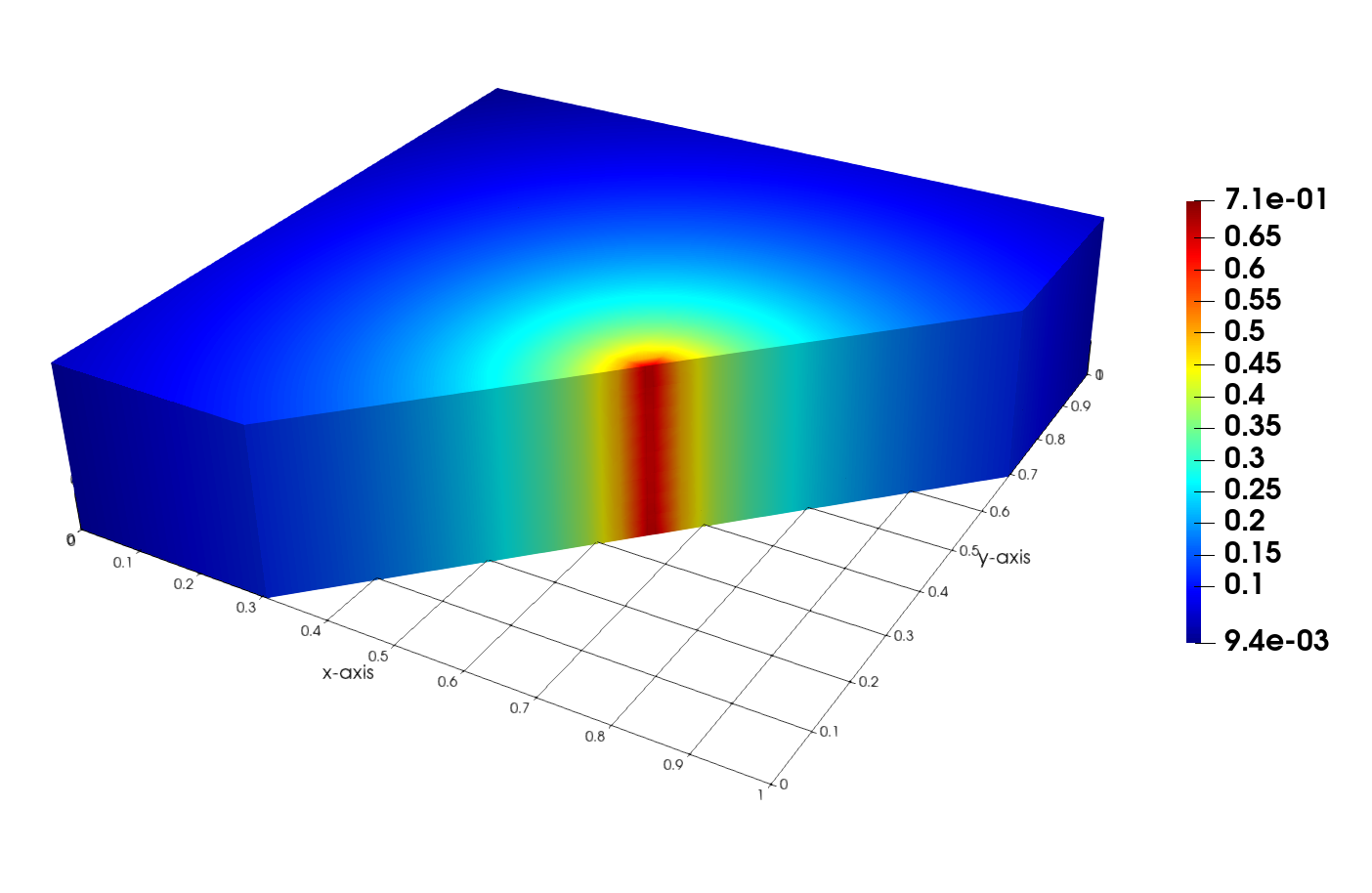
Figure 1. View on sliced domain of the dG approximation obtained on mesh of size $h=1/16$.

To show the robustness of the scheme 3.9, we now consider a sinusoidal-like curve $\Lambda$ made of segments. The numerical parameters are the same as for the manufactured solution but here, we do not know the exact solution. Figure 2 displays the DG solution on a mesh of size $h=1/10$.

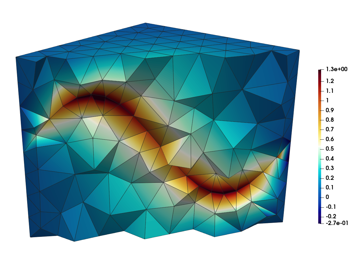
Figure 2. Sliced view of the numerical solution for a piecewise linear curve $\Lambda$.

		$\mathbf{\|u-u_{h}^{\mathrm{DG}}\|_{L^{2}(\Omega)}}$		$\mathbf{\|u-u_{h}^{\mathrm{DG}}\|_{L^{2}(C_{1})}}$		$\mathbf{\|u-u_{h}^{\mathrm{DG}}\|_{L^{2}(C_{2})}}$
k	h	Error	Rate	Error	Rate	Error	Rate
1	1/4	6.99e-03		1.28e-04		2.54e-05
	1/8	2.28e-03	1.31	3.00e-05	2.09	6.70e-06	1.92
	1/16	1.33e-03	1.08	6.60e-06	2.18	1.84e-06	1.86
	1/32	7.12e-04	0.90	1.63e-06	2.02	5.05e-07	1.87
2	1/4	1.14e-02		1.09e-04		4.37e-06
	1/8	4.27e-03	1.42	1.98e-05	2.46	7.48e-07	2.55
	1/16	1.56e-03	1.45	6.22e-06	1.67	1.11e-07	2.75
	1/32	6.14e-04	1.35	1.50e-06	2.05	1.77e-08	2.65

Table 1. Numerical errors and convergence rates for the numerical solution over the whole domain and the two subdomains.

9. Conclusions

Convergence of the class of interior penalty discontinuous Galerkin methods applied to elliptic and parabolic equations with Dirac line-source is proved by deriving error estimates in different norms. Almost optimal error bounds are shown in regions away from the line singularity. The proofs of the error estimates are technical and utilize dual problems and weighted Sobolev spaces. Stronger results are obtained for the case of piecewise linear approximation since local error bounds are valid in regions that may reach the boundary of the domain. In the general case of approximation of degree $k\geq 2$, local error bounds are subpoptimal and valid in regions strictly included in the domain. Most of the paper is dedicated to the analysis of the elliptic problem and convexity of the domain is assumed. For the parabolic problem, global error bounds in $L^{2}$ in time and in space are shown. Future work would address relaxing the convexity assumption and obtaining local error bounds for the time-dependent problem.

Acknowledgment: the authors are partially supported by NSF-DMS 1913291 and NSF-DMS 2111459.

References

- [1] Robert A. Adams and John J.F. Fournier. Sobolev Spaces. Elsevier, 2003.
- [2] Sadjia Ariche, Colette De Coster, and Serge Nicaise. Regularity of solutions of elliptic problems with a curved fracture. Journal of Mathematical Analysis and Applications, 447(2):908–932, 2017.
- [3] Silvia Bertoluzza, Astrid Decoene, Loïc Lacouture, and Sébastien Martin. Local error estimates of the finite element method for an elliptic problem with a Dirac source term. Numerical Methods for Partial Differential Equations, 34(1):97–120, 2018.
- [4] Susanne Brenner and Ridgway Scott. The Mathematical Theory of Finite Element Methods, volume 15. Springer Science & Business Media, 2007.
- [5] Eduardo Casas. estimates for the finite element method for the Dirichlet problem with singular data. Numerische Mathematik, 47(4):627–632, 1985.
- [6] Laura Cattaneo and Paolo Zunino. A computational model of drug delivery through microcirculation to compare different tumor treatments. International Journal for Numerical Methods in Biomedical Engineering, 30(11):1347–1371, 2014.
- [7] Zhangxin Chen and Hongsen Chen. Pointwise error estimates of discontinuous Galerkin methods with penalty for second-order elliptic problems. SIAM Journal on Numerical Analysis, 42(3):1146–1166, 2004.
- [8] Woocheol Choi and Sanghyun Lee. Optimal error estimate of elliptic problems with Dirac sources for discontinuous and enriched Galerkin methods. Applied Numerical Mathematics, 150:76–104, 2020.
- [9] Konstantinos Chrysafinos and L. Steven Hou. Error estimates for semidiscrete finite element approximations of linear and semilinear parabolic equations under minimal regularity assumptions. SIAM Journal on Numerical Analysis, 40(1):282–306, 2002.
- [10] Philippe G. Ciarlet. The Finite Element Method for Elliptic Problems. SIAM, 2002.
- [11] Carlo D’Angelo. Multiscale modelling of metabolism and transport phenomena in living tissues. Technical report, EPFL, 2007.
- [12] Carlo D’Angelo. Finite element approximation of elliptic problems with Dirac measure terms in weighted spaces: applications to one-and three-dimensional coupled problems. SIAM Journal on Numerical Analysis, 50(1):194–215, 2012.
- [13] Carlo D’Angelo and Alfio Quarteroni. On the coupling of 1D and 3D diffusion-reaction equations: Application to tissue perfusion problems. Mathematical Models and Methods in Applied Sciences, 18(08):1481–1504, 2008.
- [14] Michel C. Delfour and Jean-Paul Zolésio. Shape analysis via oriented distance functions. Journal of Functional Analysis, 123(1):129–201, 1994.
- [15] Daniele Di Pietro and Alexandre Ern. Discrete functional analysis tools for discontinuous Galerkin methods with application to the incompressible Navier-Stokes equations. Mathematics of Computation, 79(271):1303–1330, 2010.
- [16] Irene Drelichman, Ricardo G. Durán, and Ignacio Ojea. A weighted setting for the numerical approximation of the Poisson problem with singular sources. SIAM Journal on Numerical Analysis, 58(1):590–606, 2020.
- [17] Ricardo G. Durán and Fernando López García. Solutions of the divergence and analysis of the stokes equations in planar Hölder- domains. Mathematical Models and Methods in Applied Sciences, 20(01):95–120, 2010.
- [18] Lawrence C. Evans. Partial Differential Equations. American Mathematical Society, 2010.
- [19] David Gilbarg and Neil S. Trudinger. Elliptic Partial Differential Equations of Second Order. springer, 2015.
- [20] Ingeborg G. Gjerde, Kundan Kumar, and Jan M. Nordbotten. A singularity removal method for coupled 1D–3D flow models. Computational Geosciences, 24(2):443–457, 2020.
- [21] Ingeborg G. Gjerde, Kundan Kumar, Jan M. Nordbotten, and Barbara Wohlmuth. Splitting method for elliptic equations with line sources. ESAIM: Mathematical Modelling and Numerical Analysis, 53(5):1715–1739, 2019.
- [22] Wei Gong. Error estimates for finite element approximations of parabolic equations with measure data. Mathematics of Computation, 82(281):69–98, 2013.
- [23] Wei Gong, Gengsheng Wang, and Ningning Yan. Approximations of elliptic optimal control problems with controls acting on a lower dimensional manifold. SIAM Journal on Control and Optimization, 52(3):2008–2035, 2014.
- [24] Wei Gong and Ningning Yan. Finite element approximations of parabolic optimal control problems with controls acting on a lower dimensional manifold. SIAM Journal on Numerical Analysis, 54(2):1229–1262, 2016.
- [25] Paul Houston and Thomas P. Wihler. Discontinuous Galerkin methods for problems with Dirac delta source. ESAIM: Mathematical Modelling and Numerical Analysis-Modélisation Mathématique et Analyse Numérique, 46(6):1467–1483, 2012.
- [26] Tobias Köppl, Ettore Vidotto, and Barbara Wohlmuth. A local error estimate for the Poisson equation with a line source term. In Numerical Mathematics and Advanced Applications ENUMATH 2015, pages 421–429. Springer, 2016.
- [27] Tobias Köppl and Barbara Wohlmuth. Optimal a priori error estimates for an elliptic problem with Dirac right-hand side. SIAM Journal on Numerical Analysis, 52(4):1753–1769, 2014.
- [28] Phuong Anh Nguyen and Jean-Pierre Raymond. Control problems for convection-diffusion equations with control localized on manifolds. ESAIM: Control, Optimisation and Calculus of Variations, 6:467–488, 2001.
- [29] Joachim A. Nitsche and Alfred H. Schatz. Interior estimates for Ritz-Galerkin methods. Mathematics of Computation, 28(128):937–958, 1974.
- [30] Ricardo H. Nochetto, Enrique Otárola, and Abner J. Salgado. Piecewise polynomial interpolation in Muckenhoupt weighted Sobolev spaces and applications. Numerische Mathematik, 132(1):85–130, 2016.
- [31] Ignacio Ojea. Optimal a priori error estimates in weighted Sobolev spaces for the Poisson problem with singular sources. ESAIM: Mathematical Modelling and Numerical Analysis, 55, 2021.
- [32] Beatrice Riviere. Discontinuous Galerkin Methods for Solving Elliptic and Parabolic Equations: Theory and Implementation. SIAM, 2008.
- [33] Ridgway Scott. Finite element convergence for singular data. Numerische Mathematik, 21(4):317–327, 1973.
- [34] Vidar Thomée. Galerkin finite element methods for parabolic problems, volume 25. Springer Science & Business Media, 2007.
- [35] Lars B. Wahlbin. Local behavior in finite element methods. Handbook of Numerical Analysis, 2:353–522, 1991.
- [36] Christian Waluga and Barbara Wohlmuth. Quasi-optimal a priori interface error bounds and a posteriori estimates for the interior penalty method. SIAM Journal on Numerical Analysis, 51(6):3259–3279, 2013.