Bayesian Optimization for Macro Placement

Macro placement is the problem of placing memory blocks on a chip canvas. It can be formulated as a combinatorial optimization problem over sequence pairs, a representation which describes the relative positions of macros. Solving this problem is particularly challenging since the objective function is expensive to evaluate. In this paper, we develop a novel approach to macro placement using Bayesian optimization (BO) over sequence pairs. BO is a machine learning technique that uses a probabilistic surrogate model and an acquisition function that balances exploration and exploitation to efficiently optimize a black-box objective function. BO is more sample-efficient than reinforcement learning and therefore can be used with more realistic objectives. Additionally, the ability to learn from data and adapt the algorithm to the objective function makes BO an appealing alternative to other black-box optimization methods such as simulated annealing, which relies on problem-dependent heuristics and parameter-tuning. We benchmark our algorithm on the fixed-outline macro placement problem with the half-perimeter wire length objective and demonstrate competitive performance.

Keywords: Bayesian optimization, Permutation, Batch acquisition, Physical design, Macro Placement, Sequence Pair

1 Introduction

In chip placement two different types of objects are placed on a chip canvas: macros, which are large memory blocks, and standard cells, which are small gates performing logical operations. Compared to macros, standard cells are typically thousands of times smaller but tens or hundreds of thousands of times more numerous. While standard cell placement can be efficiently solved using continuous optimization, e.g. (Cheng et al., 2019), macro placement is typically framed as a combinatorial optimization problem due to their larger physical size. This involves searching over the discrete set of relative positions between pairs of macros, e.g. whether macro $i$ is to the left or right of macro $j$, which act as constraints against overlapping macros. The most popular combinatorial representation of relative positions is called the sequence pair which is composed of a pair of permutations, one per spatial dimension (Murata et al., 1996).

The goal of macro placement is to place macros in such a way that the power, performance and area metrics are jointly optimized. The combinatorial nature and varying sizes of macros and standard cells, together with the cost of evaluating the objective function (several days for complex designs), make macro placement a notoriously challenging step in physical design. Macro placement is also related to floorplanning, where standard cells are clustered in soft rectangles that are jointly placed with hard rectangles that represent macros (Kahng et al., 2011). In practice, designers manually place macros based on their intuition which is likely sub-optimal.

Machine learning algorithms offer an advantage over traditional optimization algorithms for macro placement since they can learn from past designs and improve over time in an automated fashion, adapting the algorithms to specific use cases. Applying machine learning to physical design has therefore recently emerged as a main research effort in electronic design automation (Kahng, 2018). In particular, reinforcement learning (RL) provides a natural framework for automating design decisions, where an agent plays the role of a designer in carefully selecting parameter configurations to evaluate next while searching for optimal solutions. However, in practice applying RL is very costly because of the large number of samples required for learning a good policy, due in part to the very large design space and costly evaluation as remarked above. For this reason, to the best of our knowledge, applications of RL in the literature are either limited to a handful of parameters (Agnesina et al., 2020) or require the use of cheap proxies instead of the real objective (Mirhoseini et al., 2020), which changes the focus towards designing good proxies.

Bayesian optimization (BO) is a technique that is well-known for its sample-efficiency, whereby it carefully explores the optimization landscape through selecting a candidate based on previous evaluations (Shahriari et al., 2015). Compared with other black-box function optimization methods such as RL, genetic algorithms, or simulated annealing (SA), the sample efficiency of BO allows flexibility for the macro placement. Especially when it is desirable to perform optimization close to the real objective, not a proxy, inevitable evaluation cost leaves only BO as a viable option. For the application to macro placement, more relevant is BO on combinatorial structures (Baptista and Poloczek, 2018; Oh et al., 2019; Deshwal et al., 2021; Deshwal and Doppa, 2021; Oh et al., 2021; Deshwal et al., 2022). For the details on BO on combinatorial structures, please refer to the references.

Contributions In this paper we introduce BO on sequence pairs for macro placement as a replacement for other black-box optimization methods such as SA which are routinely applied in the literature (Adya and Markov, 2002, 2005). We use batch BO for parallel evaluation of a batch of data points to accelerate the optimization. Fig. 1 summarizes our workflow.

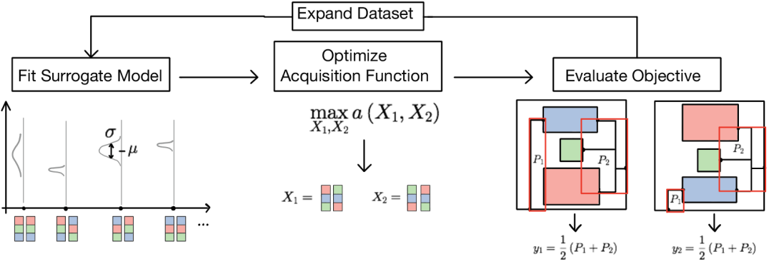
Figure 1: The Bayesian optimization for macro placement workflow for $N=3$ macros and batch size $B=2$. First we fit a surrogate model (Gaussian process) to the data, updating the mean $\mu$ and standard deviation $\sigma$ of the cost function estimate for each sequence pair, here represented as a pair of $N$ dimensional arrays where permutations correspond to different colors patterns. Then we optimize an acquisition function $a$ conditioned on the data observed so far to find new sequence pairs $x_{1},\dots,x_{B}$. Next we evaluate $x_{1},\dots,x_{B}$ by placing macros to minimize HPWL while respecting the sequence pair constraints, and compute the corresponding objective values $y_{1},\dots,y_{B}$. Here $P_{i}$ is the perimeter of the $i$-th bounding box of the net between macros and I/O pads. Finally we add these new points to the dataset and repeat the procedure until the computational budget is exhausted.

Our main contributions are:

• We extend batch BO on permutations (Oh et al., 2021) to batch BO on sequence pairs and devise an efficient algorithm for parallel batch acquisition function optimisation.

• We benchmark our algorithm on the MCNC dataset and obtain superior performance in terms of wire length metric as compared to SA.

2 Methodology

In contrast to the traditional macro placement approaches, we consider an expensive-to-evaluate objective with which we perform macro placement. We also consider the fixed-outline constraint addressed in many existing works (Adya and Markov, 2001).

In order to efficiently tackle macro placement, we employ batch BO on the space of sequence pairs (SPs) – a pair of two permutations – a compact representation for the relative positions of macros. Sequence pairs describe non-overlapping placements of macros. Intuitively, if we imagine the macros to be placed on a line, the space of non-overlapping placements can be indexed by permutations of the macros, and a macro optimization problem with non-overlapping constraints can be solved by searching over the space of permutations. In the two-dimensional setting of this paper we need a pair of permutation to describe non-overlapping macro placements. See Appx. Subsec. B.1 and (Murata et al., 1996) for detailed explanation. To this end, we introduce 1) a kernel on the space of SPs, 2) an efficient heuristic to optimize the batch acquisition function 3) an efficient vectorized Python implementation of the least common subsequence (LCS) algorithm of $O(N\log N)$ run-time complexity where $N$ is the number of macros.

For our Gaussian process surrogate model in BO, the proposed kernel is based on the position kernel on permutation due to its superior performance in (batch) BO on permutation spaces(Zaefferer et al., 2014; Oh et al., 2021). Denoted $\pi_{1},\pi_{2},\pi_{1}^{\prime},\pi_{2}^{\prime}$ four permutations of $N$ elements, our kernel is:

$$K_{sp}((\pi_{1},\pi^{\prime}_{1}),(\pi_{2},\pi^{\prime}_{2})|\mathbf{W},\mathbf{W}^{\prime})=K_{perm}(\pi_{1},\pi_{2}|\mathbf{W})\cdot K_{perm}(\pi^{\prime}_{1},\pi^{\prime}_{2}|\mathbf{W}^{\prime})$$ (1)

where $\mathbf{W}=[w_{1},\cdots,w_{N}]$, $\mathbf{W}^{\prime}=[w^{\prime}_{1},\cdots,w^{\prime}_{N}]$, and

$$K_{perm}(\pi_{1},\pi_{2}|w_{1},\cdots,w_{N})=\exp{\Big{(}\sum_{n=1}^{N}}w_{n}\cdot|\pi_{1}^{-1}(n)-\pi_{2}^{-1}(n)|\Big{)}$$

$K_{perm}(\pi_{1},\pi_{2}|1,\cdots,1)$ is the position kernel (Zaefferer et al., 2014; Oh et al., 2021). In addition to the mentioned works, in our position kernel we introduce parameters $\mathbf{W},\mathbf{W}^{\prime}$ that account for widths and heights of different macros. We optimize those parameters by maximizing the marginal likelihood of the training data by gradient descent.

In the batch acquisition function of BO, we adopt the method in (Oh et al., 2021) which uses determinantal point processes (DPPs) with a weighted kernel to obtain a batch of diverse points each of which is likely to speed up BO progress. DPPs quantify the diversity of points using determinant of the gram matrix. Since the determinant of a matrix is the volume of hyper-parallelepiped whose vertices are columns of the matrix, the more diverse the points are, the larger the determinant is (Kulesza and Taskar, 2011, 2012). The batch acquisition function is defined as

$$a^{(t)}_{batch}(x_{1},\cdots,x_{B})=\det\big{[}\rho\big{(}a^{(t)}(x_{b})\big{)}\,K^{(t)}(x_{b},x_{c})\,\rho\big{(}a^{(t)}(x_{c})\big{)}\big{]}_{b,c=1,\cdots,B}\,$$ (2)

where $K^{(t)}$ the covariance function conditioned on the evaluation dataset $\mathbf{X}^{(t)}$ as in Eq. (3), $a^{(t)}$ is the acquisition function for a single point as in Eq. (4) (e.g. EI, UCB, EST(Wang et al., 2016)), and $\rho(\cdot)$ is a positive and strictly increasing function. This batch acquisition function balances the quality of each point (i.e. the likelihood of improving the objective) through the acquisition weight $\rho\big{(}a^{(t)}(\cdot)\big{)}$, and the diversity among points (i.e. avoiding information redundancy in parallel evaluations) through $K^{(t)}$. This function has been demonstrated to perform well for BO on permutation spaces(Oh et al., 2021).

While $a^{(t)}_{batch}$ effectively fulfills the quality and diversity requirements, its optimization is computationally demanding. In (Oh et al., 2021), a greedy approach was employed with certain optimality guarantees. However, that method optimizes $a^{(t)}_{batch}$ sequentially over the batch index and limits the scalability of batch BO. Therefore, we propose a new heuristic for parallel optimization of the batch acquisition function (See Alg. 1 in Appx. Sec. C)

The main idea is to perform small local updates in parallel for each element of the batch. Specifically, we first compute $x_{opt,1}$, the optimum of the single point acquisition function (See line no. 1 of Alg. 1 in Appx. Sec. C). Then we optimize the function $a_{s,b}$ defined by fixing all but the $b$-th element of the batch, for $b=2,\dots,B$ (See line no. 6 of Alg. 1 in Appx. Sec. C Alg. 1). This step can be parallelized over the batch. Here $s$ denotes the iteration time over which this procedure is repeated. When a single point is updated (line no. 1 of Alg. 1 in Appx. Sec. C), we apply a small local update instead of running until convergence to minimize the deviation of our individual updates from the simultaneous update method. Intuitively, if any single point is significantly altered while the rest is fixed, the end result of the individual updates will drastically differ from that of the simultaneous update.

The parallel heuristic (Alg. 1 in Appx. Sec. C) takes as input a local update function. The local update function (Alg. 2 in Appx. Sec. C ) checks the constraint of fixed outline of the placement region. We call feasible SPs those SPs that fit into the placement region.

By using Alg. 2 (Appx. Sec. C) as the local update function for the parallel heuristic (Alg. 1 in Appx. Sec. C), the latter collects feasible points by accumulating the feasible sets generated by the former. When the local update function (Alg. 2 in Appx. Sec. C) is invoked in the parallel heuristic (Alg. 1 in Appx. Sec. C), $c_{feasible}(\cdot)$ is the function which asserts the fixed-outline constraint using the LCS algorithm, and $\mathcal{N}(x)$ is the set of neighbors of the sequence pair $x$ obtained by swapping adjacent elements in each permutation.

Given the kernel $K_{sp}$, the batch acquisition function, and the parallel heuristic for its optimization, we present the complete Bayesian optimization for macro placement workflow in Alg. 3 in Appx. Sec. C. See also Fig. 1 for a graphical illustration.

3 Experiments

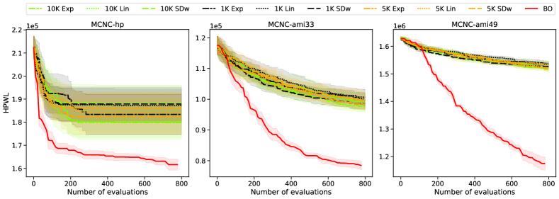
Figure 2: BO vs. SA on MCNC (hp, ami33, ami49) across temperatures (1K, 5K, 10K) and schedules (linear, exponential, stepdown)

As a demonstration of the potential of BO, we test it on the MCNC benchmark (Kozminski, 1991) and present the results in Tab. 1. The optimization objective is to minimize HPWL which connects macros pins to I/O pads under the fixed-outline constraint. Note that I/O pads are fixed on the boundary of the placement region. Under the relative location constraints specified by a sequence pair, we perform the linear constrained programming to minimize HPWL. Note that this objective is simpler and cheaper-to-evaluate than the ones where BO can possibly show its full strengths. Nonetheless, this experiment does indicate the potential of BO in macro placement.

Table 1: HPWL results on the MCNC benchmark. (The number of macros in parentheses)

	apte (9)	xerox (10)	hp (11)	ami33 (33)	ami49 (49)
eWL(Funke et al., 2016)	513,061	370,993	153,328	58,627	640,509
ELS (Liu and Nannarelli, 2008)	614,602	404,278	253,366	96,205	1,070,010
FDa (Samaranayake et al., 2009)	545,136	755,410	155,463	63,125	871,128
SAb,d	515,570	431,108	179,826	97,691	1,517,051
	$\pm$525	$\pm$15,312	$\pm$6,550	$\pm$1,592	$\pm$5,095
	1e3, Exp	1e3, Lin	1e4, Exp	1e4, Exp	1e4, Lin
BOc,d	514,138	388,936	161,620	78,359	1,174,972
	$\pm$264	$\pm$3,700	$\pm$2,113	$\pm$1,271	$\pm$21,396

• Packings for hp, ami33, and ami49 have overlaps.

• Among different temperature scheduling, the result with the lowest mean is reported.

• BO uses the batch size $B=10$

• Mean and standard error of 5 runs are reported.

In Tab. 1, we compare the black-box function optimizers (BO, SA) with other methods in the literature on all 5 MCNC problems. In Fig 2, we compare BO and SA with different temperature scheduling for 3 largest problems. For all problems, BO has superior performance for the same number of evaluations, with the gap growing larger for larger number of macros. In comparison with the other methods of Tab. 1, we can see that BO performs competitively with only 520 evaluations of the objective on apte which is the smallest problem. We acknowledge that on the designs with a larger number of macros, ami33 and ami49, there is a non-negligible gap between BO and eWL (Funke et al., 2016). However, we expect that this gap does not translate to the real world applications that we envision since eWL cannot optimize macro placements with standard cells, while BO and SA can. This is because eWL relies on efficient HPWL evaluation and uses a far higher number of evaluations. Moreover, for apte, xerox, hp, eWL performed an exhaustive search. On the other hand, due to super-exponential size of the space of sequence pairs on ami33 and ami49, evaluations are not performed exhaustively but nevertheless are many orders of magnitude larger than the number of BO evaluations. In comparison with ELS (Liu and Nannarelli, 2008), BO outperforms in all but ami49. However, ELS is a SA tuned for a specific proxy cost function and we expect it not to be transferable to optimize more general and expensive cost functions. Further, in spite of extremely small number of evaluations compared with the size of the search space in ami49, BO demonstrates its potential for more general and more realistic objectives on such large number of macros. FD (Samaranayake et al., 2009) outperforms BO on hp, ami33, ami49 but the macro locations that FD outputs have overlaps, while our method does not.

4 Conclusions

In this paper, we demonstrated the effectiveness of Bayesian optimization for macro placement, and have shown that it performs competitively with exhaustive search techniques on small benchmarks and performs reasonably well within compute constraints for large benchmarks. In comparison to simulated annealing, we have shown our BO framework to outperform across benchmarks with fewer evaluations. As mentioned above, realistic macro placement quality evaluation requires an expensive global placement loop. Our optimization objective in the experiments was to minimize HPWL of macro to I/O pads connections which helped us evaluate macro placement quality without standard cell placement in the loop. In the future, we plan 1) to extend this framework with an objective that considers standard cell placement for HPWL computation and congestion estimation 2) to utilize the current work’s output as initial solution to macro placement with subsequent standard cell placement 3) to extend our constraints with memory stacking requirements, dataflow constraints, channel and snapping constraints, which are typical in industry standard IPs. On the machine learning front, a future challenge is to develop a BO framework that transfers across designs.

A Related Work

Sequential macro placers (Markov et al., 2015; Adya and Markov, 2002, 2005) produce overlap-free placements for macros in four steps: 1. cluster standard cells into soft rectangles, 2. run a floorplanner on the original (hard) macros and new soft rectangles, 3. remove the soft rectangles, 4. place standard cells with fixed macros. The floorplanner of choice is typically based on SA over sequence pairs with the most popular implementation being Parquet (Adya and Markov, 2001) which incorporates several heuristics to select new configurations. Modern sequential workflows such as the Triton macro placer included in the OpenRoad project (ope, 2021) use RePlace (Cheng et al., 2019) for standard cell placement. Replace is a state-of-the-art academic analytical placer that uses an electrostatic analogy whereby cells and macros are modelled as charged objects with charges proportional to their areas, and their electrostatic equilibrium leads to a uniformly spread placement. Performing joint macro and standard cell placement using RePlace produces overlaps that must be later removed by a legalization step, as done in (Lu et al., 2015) that also uses SA.

In all the aforementioned workflows we can replace SA with our BO algorithm. SA requires many iterations to converge and does not scale when using realistic cost functions, which limits the choice of cost functions that designers can feasibly use for SA and thus may lead to important aspects of the problem being ignored. Furthermore, SA requires the designer to carefully adjust parameters such as temperature schedule and acceptance probability to obtain good results – though (Vashisht et al., 2020) proposes an algorithm that learns to propose good initial values. In contrast, in BO the kernel hyperparameters can be tuned automatically by fitting the training data with gradient-based optimization. Nevertheless, acquisition function maximization in our combinatorial setting requires some tuning, see Sec. 2.

Various techniques other than SA have been proposed for floorplanning. In (Funke et al., 2016) an exact enumeration algorithm is applied to larger problems using a divide-and-conquer strategy. However, this method can only be applied to the half-perimeter wire length objective and not more realistic cost functions. Similarly, (Liu and Nannarelli, 2008; Samaranayake et al., 2009) also use wire length proxy functions.

A closely-related work to ours uses RL for macro placement (Mirhoseini et al., 2020). RL requires many training iterations to converge to a good policy, while BO is more data-efficient and is therefore more appealing when evaluating an expensive reward function. In contrast to RL, BO does not learn to act in multiple situations, meaning that each new design requires optimization from scratch. BO can be seen as a simplified instance of RL where one takes a single action (instead of a sequence of actions) in a fixed state (i.e. bandits) (Sutton and Barto, 2018; Srinivas et al., 2009; Chowdhury and Gopalan, 2017). Other practical differences of our work and (Mirhoseini et al., 2020) are: 1) their RL agent places macros sequentially while we jointly place all macros as done in SA; 2) they discretize the macro positions on a fictitious grid while we work in the exact continuum optimization formulation with no overlap constraints. In Sec.3 we compared our results against our SA implementation and previously reported methods on the same benchmark dataset. We leave benchmarking against (Mirhoseini et al., 2020) as future work.

Recently, BO was tested on similar but much smaller cases in (Deshwal et al., 2022). Their focus is on proposing a new kernel on permutations and it is orthogonal to our focus on the batch acquisition to tackle super-exponential growth. In contrast to (Deshwal et al., 2022), our experiments were conducted on much larger spaces i.e., 3$\sim$4 times more macros – in terms of the size of search space, this makes huge difference due to super-exponential growth of permutation spaces – and demonstrated the effectiveness of the batch acquisition. We leave the search for the optimal combination of the kernel and the batch acquisition for macro placement as a future work.

Finally, we note that in (Xu et al., 2017) a bandit-based approach similar to BO has been applied to optimizing parameters of FPGA compilation. This work does not tackle the challenges of large combinatorial spaces in macro placement.

B Background

B.1 Sequence pair

Sequence pairs (SPs) were introduced in (Murata et al., 1996) as a combinatorial representation for macro packing problems. We recall that a macro is a rectangle with distinguished points called pins which may connect wires. For macros $\{m_{1},\cdots,m_{N}\}$, an SP is a pair of permutations of length $N$, one per spatial dimension, and specifies the relative location of each pair of macros. The relationship between the four possible relative locations of macros $m_{i}$ and $m_{j}$ and SPs are explained in Tab. 2.

Table 2: Relative location specified by sequence pair $(\pi,\pi^{\prime})$

$\pi$	$\pi^{\prime}$	Relative location of $i$ and $j$
$(\cdots,i,\cdots,j,\cdots)$	$(\cdots,i,\cdots,j,\cdots)$	$i$ is to the left of $j$
$(\cdots,j,\cdots,i,\cdots)$	$(\cdots,j,\cdots,i,\cdots)$	$i$ is to the right of $j$
$(\cdots,i,\cdots,j,\cdots)$	$(\cdots,j,\cdots,i,\cdots)$	$i$ is below $j$
$(\cdots,j,\cdots,i,\cdots)$	$(\cdots,i,\cdots,j,\cdots)$	$i$ is above $j$

Traditionally, the SP representation has been used in macro placement for optimizing area and half perimeter wire length (HPWL) (Murata et al., 1996). HPWL is the half perimeter of the bounding box around a net (e.g. the red boxes in Fig. 1). To convert the SP to a packed placement, an algorithm called the Longest Common Subsequence (LCS) is used. It ensures minimal area placement, where no further vertical or horizontal adjustment of any macro is possible (Murata et al., 1996).

Simulated annealing (SA) is commonly used to search over the space of SPs by carefully-designed stochastic moves (Adya and Markov, 2001). The optimization objective is typically a linear combination of area and HPWL. The conversion from an SP to a placement is the main computational bottleneck. Since SA requires several thousands of evaluations to find a good solution, a cheap proxy for the objective that relies on LCS is used in practice (Adya and Markov, 2001). Another direction of work focused on the efficient LCS implementations to handle this computational bottleneck (Tang and Wong, 2001; Tang et al., 2001). In contrast, our work aims to optimize a complex and expensive objective through a BO routine, while using LCS to assert whether an SP can be converted to a placement which fits within the fixed placement region.

B.2 Bayesian optimization

BO has been widely successful in optimizing expensive-to-evaluate objectives such as hyperparameter optimization (Snoek et al., 2015), neural architecture search (Nguyen et al., 2021) and optimization of the tokamak control for nuclear fusion (Char et al., 2019). The superior sample efficiency of BO is attributed to two components, namely the surrogate model and the acquisition function. The surrogate model is a probabilistic model that approximates the objective while measuring the uncertainty of its approximation. This uncertainty plays a crucial role in the exploration-exploitation trade-off. For this reason, Gaussian processes (GPs) are widely used due to their superior uncertainty quantification (Rasmussen, 2003; Snoek et al., 2012). Given a point $x$ in the search space, at the $t$-th iteration of BO, the predictive mean $\mu_{t}(x)$ and the predictive covariance $K^{(t)}(x,x^{\prime})$ of the GP surrogate model are defined as

$$\mu_{t}(x)=m_{x}+K_{x,\mathbf{X}^{(t)}}(K_{\mathbf{X}^{(t)},\mathbf{X}^{(t)}}+\sigma^{2}I)^{-1}(\mathbf{y}^{(t)}-m_{\mathbf{X}^{(t)}})$$

$$K^{(t)}(x,x^{\prime})\!=\!K_{x,x^{\prime}}-K_{x,\mathbf{X}^{(t)}}(K_{\mathbf{X}^{(t)},\mathbf{X}^{(t)}}\!+\!\sigma^{2}I)^{-1}K_{\mathbf{X}^{(t)},x^{\prime}}$$ (3)

where $m_{\cdot}$ is the mean function, $K_{\cdot,\cdot}$ is the kernel (i.e. prior covariance function), $\sigma^{2}$ is the variance of the observational noise and $\mathbf{X}^{(t)}$ is the set of points evaluated so far. The predictive variance is $\sigma^{2}_{t}(x)=K^{(t)}(x,x)$.

Using the GP predictive distribution conditioned on the evaluation dataset $(\mathbf{X}^{(t)},\mathbf{y}^{(t)})$, the acquisition function $a(\cdot,\cdot)$ quantifies the chance that the evaluation of a point improves the GP optimization. An acquisition function is based on the intuition that the predictive mean and the predictive variance can be used to make an informed guess about the usefulness of a point in the input space (Shahriari et al., 2015):

$$a^{(t)}(x)=a(\mu_{t}(x),\sigma^{2}_{t}(x))\,.$$ (4)

In general, the acquisition function value is higher at points where the predictive mean and the predictive variance are relatively high. The argument of the maximum of the acquisition function $x^{(t)}_{opt}$ is evaluated under the true objective $y^{(t)}=f(x^{(t)}_{opt})$. This new datapoint is then added to the evaluation dataset and the BO process is repeated.

$$\mathbf{X}^{(t+1)}=[\mathbf{X}^{(t)};x^{(t)}_{opt}],\,\,\,\,\mathbf{y}^{(t+1)}=[\mathbf{y}^{(t)};y^{(t)}]$$ (5)

BO can be accelerated when computational resources permit parallel evaluation of the objective. In this case, the acquisition function is defined over multiple points so that its optimization yields multiple points whose evaluation can be parallelized.

$$\{x^{(t)}_{opt,b}\}_{b=1}^{B}=\operatorname{argmax}_{x_{1},\cdots,x_{B}}a^{(t)}_{batch}(x_{1},\cdots,x_{B})$$ (6)

This is called batch BO. Several works have proposed methods which use different batch acquisition functions(González et al., 2016; Wu and Frazier, 2016; Lyu et al., 2018; Gong et al., 2019). For a detailed overview of BO, the reader is referred to (Brochu et al., 2010; Shahriari et al., 2015; Frazier, 2018).

C Algorithms

Algorithm 1 Parallel heuristic

0:  $a$ : an acquisition function for a single point$a_{batch}$ : a batch acquisition function $u_{local}(g(\cdot),x)$ : a local update function        such that $g(u_{local}(g(\cdot),x))\geq g(x)$(maximization) $\mathbf{X}_{feasible}$ : a feasible set

1:  $x_{opt,1}=\operatorname{argmax}_{x\in\mathbf{X}_{feasible}}a(x)$

2:  Randomly choose $x_{0,b}$ for $b=2,\cdots,B$ from $\mathbf{X}_{feasible}$

3:  repeat

4:     $\mathbf{X}_{feasible,s}=\emptyset$

5:     for $b\in\{2,\cdots,B\}$ do {Parallel}

6:        Update $x_{s,b}$ $a_{s,b}(x)=a_{batch}(x_{opt,1},x_{s,2},\cdots,x_{s,b-1},x,x_{s,b+1},\cdots)$$x_{s+1,b},\mathbf{X}_{feasible,s,b}=u_{local}(a_{s,b}(\cdot),x_{s,b})$

7:        Collect feasible sets $\mathbf{X}_{feasible,s}=\mathbf{X}_{feasible,s}\cup\mathbf{X}_{feasible,s,b}$

8:     end for

9:     Expand the feasible set$\mathbf{X}_{feasible}=\mathbf{X}_{feasible}\cup\mathbf{X}_{feasible,s}$

10:     Update step count $s=s+1$

11:  until Convergence or other stopping criteria

12:  return  $(x_{opt,1},x_{\cdot,2},\cdots,x_{\cdot,B}),\mathbf{X}_{feasible}$

Algorithm 2 Local update with feasibility check

0:  $g(x)$ : an objective function $x_{old}$ : an initial point $c_{feasible}(x)$ : a function checking the feasibility$\mathcal{N}(x)$ : a function listing neighbors of $x$

1:  Find neighbors of $x_{old}$, $\mathcal{N}(x_{old})$

2:  Compute feasibility$\mathcal{N}_{feasible}(x_{old})=\{x\in\mathcal{N}(x_{old})\,|\,c_{feasible}(x)~{}\text{is true}\}$

3:  Move toward the best feasible neighbor$x_{new}=\operatorname{opt}_{x\in\mathcal{N}_{feasible}(x_{old})}g(x)$

4:  Expand the feasible set$X_{feasible}=X_{feasible}\cup\mathcal{N}_{feasible}(x_{old})$

5:  return  $x_{new},X_{feasible}$

Algorithm 3 Batch Bayesian optimization macro placement

0:  $f$ : the optimization objective $\mathbf{X}^{(0)}_{feasible}$ : an initial feasible set $\mathbf{X}^{(0)},\mathbf{y}^{(0)}$ : an initial evaluation dataset

1:  repeat

2:     Fit the surrogate model on the data ($\mathbf{X}^{(t)}$, $\mathbf{y}^{(t)}$)$\mu_{t}(x)$, $\sigma^{2}_{t}(x)$        [Used in the acquisition function]

3:     Optimize the acquisition function by calling Alg. 1 with - Local update fn.: Alg. 2 - Feasible set: $\mathbf{X}^{(t)}_{feasible}$ $(x^{(t)}_{1},\cdots,x^{(t)}_{B})$, $\mathbf{X}^{new}_{feasible}\leftarrow$ Alg. 1

4:     Evaluate the objective at $(x^{(t)}_{1},\cdots,x^{(t)}_{B})$ in parallel $y^{(t)}_{1}=f(x^{(t)}_{1}),\cdots,y^{(t)}_{B}=f(x^{(t)}_{B})$

5:     Expand the evaluation dataset $\mathbf{X}^{(t+1)}=[\mathbf{X}^{(t)};x^{(t)}_{1};\cdots;x^{(t)}_{B}]$$\mathbf{y}^{(t+1)}=[\mathbf{y}^{(t)};y^{(t)}_{1};\cdots;y^{(t)}_{B}]$

6:     Expand the feasible set $\mathbf{X}^{(t+1)}_{feasible}=\mathbf{X}^{(t)}_{feasible}\cup\mathbf{X}^{new}_{feasible}$

7:     Update BO round count $t=t+1$

8:  until Computational budget is exhausted

9:  return  $\mathbf{X}^{(\cdot)}$, $\mathbf{y}^{(\cdot)}$

References

- ope (2021) The-openroad-project. https://github.com/The-OpenROAD-Project/OpenROAD, 2021.
- Adya and Markov (2005) S. N. Adya and Igor L. Markov. Combinatorial techniques for mixed-size placement. ACM Trans. Des. Autom. Electron. Syst., 10(1):58–90, January 2005. ISSN 1084-4309. doi: 10.1145/1044111.1044116. URL https://doi.org/10.1145/1044111.1044116.
- Adya and Markov (2002) Saurabh N Adya and Igor L Markov. Consistent placement of macro-blocks using floorplanning and standard-cell placement. In Proceedings of the 2002 International Symposium on Physical design, pages 12–17, 2002.
- Adya and Markov (2001) S.N. Adya and I.L. Markov. Fixed-outline floorplanning through better local search. In Proceedings 2001 IEEE International Conference on Computer Design: VLSI in Computers and Processors. ICCD 2001, pages 328–334, 2001. doi: 10.1109/ICCD.2001.955047.
- Agnesina et al. (2020) Anthony Agnesina, Kyungwook Chang, and Sung Kyu Lim. Vlsi placement parameter optimization using deep reinforcement learning. In 2020 IEEE/ACM International Conference On Computer Aided Design (ICCAD), pages 1–9, 2020.
- Baptista and Poloczek (2018) Ricardo Baptista and Matthias Poloczek. Bayesian optimization of combinatorial structures. In International Conference on Machine Learning, pages 462–471. PMLR, 2018.
- Brochu et al. (2010) Eric Brochu, Vlad M Cora, and Nando De Freitas. A tutorial on bayesian optimization of expensive cost functions, with application to active user modeling and hierarchical reinforcement learning. arXiv preprint arXiv:1012.2599, 2010.
- Char et al. (2019) Ian Char, Youngseog Chung, Willie Neiswanger, Kirthevasan Kandasamy, Andrew O Nelson, Mark Boyer, Egemen Kolemen, and Jeff Schneider. Offline contextual bayesian optimization. Advances in Neural Information Processing Systems, 32:4627–4638, 2019.
- Cheng et al. (2019) Chung-Kuan Cheng, Andrew B. Kahng, Ilgweon Kang, and Lutong Wang. Replace: Advancing solution quality and routability validation in global placement. IEEE Transactions on Computer-Aided Design of Integrated Circuits and Systems, 38(9):1717–1730, 2019. doi: 10.1109/TCAD.2018.2859220.
- Chowdhury and Gopalan (2017) Sayak Ray Chowdhury and Aditya Gopalan. On kernelized multi-armed bandits. In International Conference on Machine Learning, pages 844–853. PMLR, 2017.
- Deshwal and Doppa (2021) Aryan Deshwal and Jana Doppa. Combining latent space and structured kernels for bayesian optimization over combinatorial spaces. Advances in Neural Information Processing Systems, 34:8185–8200, 2021.
- Deshwal et al. (2021) Aryan Deshwal, Syrine Belakaria, and Janardhan Rao Doppa. Mercer features for efficient combinatorial bayesian optimization. In Proceedings of the AAAI Conference on Artificial Intelligence, volume 35, pages 7210–7218, 2021.
- Deshwal et al. (2022) Aryan Deshwal, Syrine Belakaria, Janardhan Rao Doppa, and Dae Hyun Kim. Bayesian optimization over permutation spaces. In Proceedings of the AAAI Conference on Artificial Intelligence, volume 36, pages 6515–6523, 2022.
- Frazier (2018) Peter I Frazier. A tutorial on bayesian optimization. arXiv preprint arXiv:1807.02811, 2018.
- Funke et al. (2016) J. Funke, S. Hougardy, and J. Schneider. An exact algorithm for wirelength optimal placements in vlsi design. Integration, 52:355–366, 2016. ISSN 0167-9260. doi: https://doi.org/10.1016/j.vlsi.2015.07.001. URL https://www.sciencedirect.com/science/article/pii/S0167926015000802.
- Gong et al. (2019) Chengyue Gong, Jian Peng, and Qiang Liu. Quantile stein variational gradient descent for batch bayesian optimization. In International Conference on Machine Learning, pages 2347–2356. PMLR, 2019.
- González et al. (2016) Javier González, Zhenwen Dai, Philipp Hennig, and Neil Lawrence. Batch bayesian optimization via local penalization. In Artificial intelligence and statistics, pages 648–657. PMLR, 2016.
- Kahng et al. (2011) A.B. Kahng, J. Lienig, I.L. Markov, and J. Hu. VLSI Physical Design: From Graph Partitioning to Timing Closure. Springer Netherlands, 2011. ISBN 9789048195916. URL https://books.google.nl/books?id=DWUGHyFVpboC.
- Kahng (2018) Andrew B Kahng. Machine learning applications in physical design: Recent results and directions. In Proceedings of the 2018 International Symposium on Physical Design, pages 68–73, 2018.
- Kozminski (1991) K. Kozminski. Benchmarks for layout synthesis - evolution and current status. In 28th ACM/IEEE Design Automation Conference, pages 265–270, 1991.
- Kulesza and Taskar (2011) Alex Kulesza and Ben Taskar. k-dpps: Fixed-size determinantal point processes. In ICML, 2011.
- Kulesza and Taskar (2012) Alex Kulesza and Ben Taskar. Determinantal point processes for machine learning. arXiv preprint arXiv:1207.6083, 2012.
- Liu and Nannarelli (2008) Wei Liu and Alberto Nannarelli. Net balanced floorplanning based on elastic energy model. In 2008 NORCHIP, pages 258–263. IEEE, 2008.
- Lu et al. (2015) Jingwei Lu, Hao Zhuang, Pengwen Chen, Hongliang Chang, Chin-Chih Chang, Yiu-Chung Wong, Lu Sha, Dennis Huang, Yufeng Luo, Chin-Chi Teng, and Chung-Kuan Cheng. eplace-ms: Electrostatics-based placement for mixed-size circuits. IEEE Transactions on Computer-Aided Design of Integrated Circuits and Systems, 34(5):685–698, 2015. doi: 10.1109/TCAD.2015.2391263.
- Lyu et al. (2018) Wenlong Lyu, Fan Yang, Changhao Yan, Dian Zhou, and Xuan Zeng. Batch bayesian optimization via multi-objective acquisition ensemble for automated analog circuit design. In International conference on machine learning, pages 3306–3314. PMLR, 2018.
- Markov et al. (2015) Igor L. Markov, Jin Hu, and Myung-Chul Kim. Progress and challenges in vlsi placement research. Proceedings of the IEEE, 103(11):1985–2003, 2015. doi: 10.1109/JPROC.2015.2478963.
- Mirhoseini et al. (2020) Azalia Mirhoseini, Anna Goldie, Mustafa Yazgan, Joe Jiang, Ebrahim Songhori, Shen Wang, Young-Joon Lee, Eric Johnson, Omkar Pathak, Sungmin Bae, Azade Nazi, Jiwoo Pak, Andy Tong, Kavya Srinivasa, William Hang, Emre Tuncer, Anand Babu, Quoc V. Le, James Laudon, Richard Ho, Roger Carpenter, and Jeff Dean. Chip placement with deep reinforcement learning, 2020.
- Murata et al. (1996) Hiroshi Murata, Kunihiro Fujiyoshi, Shigetoshi Nakatake, and Yoji Kajitani. Vlsi module placement based on rectangle-packing by the sequence-pair. IEEE Transactions on Computer-Aided Design of Integrated Circuits and Systems, 15(12):1518–1524, 1996.
- Nguyen et al. (2021) Vu Nguyen, Tam Le, Makoto Yamada, and Michael A Osborne. Optimal transport kernels for sequential and parallel neural architecture search. In International Conference on Machine Learning, pages 8084–8095. PMLR, 2021.
- Oh et al. (2019) Changyong Oh, Jakub Tomczak, Efstratios Gavves, and Max Welling. Combinatorial bayesian optimization using the graph cartesian product. Advances in Neural Information Processing Systems, 32, 2019.
- Oh et al. (2021) Changyong Oh, Roberto Bondesan, Efstratios Gavves, and Max Welling. Batch bayesian optimization on permutations using acquisition weighted kernels. arXiv preprint arXiv:2102.13382, 2021.
- Rasmussen (2003) Carl Edward Rasmussen. Gaussian processes in machine learning. In Summer school on machine learning, pages 63–71. Springer, 2003.
- Samaranayake et al. (2009) Meththa Samaranayake, Helen Ji, and John Ainscough. Development of a force directed module placement tool. In 2009 Ph. D. Research in Microelectronics and Electronics, pages 152–155. IEEE, 2009.
- Shahriari et al. (2015) Bobak Shahriari, Kevin Swersky, Ziyu Wang, Ryan P Adams, and Nando De Freitas. Taking the human out of the loop: A review of bayesian optimization. Proceedings of the IEEE, 104(1):148–175, 2015.
- Snoek et al. (2012) Jasper Snoek, Hugo Larochelle, and Ryan P Adams. Practical bayesian optimization of machine learning algorithms. Advances in neural information processing systems, 25, 2012.
- Snoek et al. (2015) Jasper Snoek, Oren Rippel, Kevin Swersky, Ryan Kiros, Nadathur Satish, Narayanan Sundaram, Mostofa Patwary, Mr Prabhat, and Ryan Adams. Scalable bayesian optimization using deep neural networks. In International conference on machine learning, pages 2171–2180. PMLR, 2015.
- Srinivas et al. (2009) Niranjan Srinivas, Andreas Krause, Sham M Kakade, and Matthias Seeger. Gaussian process optimization in the bandit setting: No regret and experimental design. arXiv preprint arXiv:0912.3995, 2009.
- Sutton and Barto (2018) Richard S Sutton and Andrew G Barto. Reinforcement learning: An introduction. MIT press, 2018.
- Tang and Wong (2001) Xiaoping Tang and DF Wong. Fast-sp: A fast algorithm for block placement based on sequence pair. In Proceedings of the 2001 Asia and South Pacific design automation conference, pages 521–526, 2001.
- Tang et al. (2001) Xiaoping Tang, Ruiqi Tian, and DF Wong. Fast evaluation of sequence pair in block placement by longest common subsequence computation. IEEE Transactions on Computer-Aided Design of Integrated Circuits and Systems, 20(12):1406–1413, 2001.
- Vashisht et al. (2020) Dhruv Vashisht, Harshit Rampal, Haiguang Liao, Yang Lu, Devika Shanbhag, Elias Fallon, and Levent Burak Kara. Placement in integrated circuits using cyclic reinforcement learning and simulated annealing. arXiv preprint arXiv:2011.07577, 2020.
- Wang et al. (2016) Zi Wang, Bolei Zhou, and Stefanie Jegelka. Optimization as estimation with gaussian processes in bandit settings. In Artificial Intelligence and Statistics, pages 1022–1031. PMLR, 2016.
- Wu and Frazier (2016) Jian Wu and Peter Frazier. The parallel knowledge gradient method for batch bayesian optimization. Advances in Neural Information Processing Systems, 29:3126–3134, 2016.
- Xu et al. (2017) Chang Xu, Gai Liu, Ritchie Zhao, Stephen Yang, Guojie Luo, and Zhiru Zhang. A parallel bandit-based approach for autotuning fpga compilation. In Proceedings of the 2017 ACM/SIGDA International Symposium on Field-Programmable Gate Arrays, FPGA ’17, page 157–166, New York, NY, USA, 2017. Association for Computing Machinery. ISBN 9781450343541. doi: 10.1145/3020078.3021747. URL https://doi.org/10.1145/3020078.3021747.
- Zaefferer et al. (2014) Martin Zaefferer, Jörg Stork, and Thomas Bartz-Beielstein. Distance measures for permutations in combinatorial efficient global optimization. In International Conference on Parallel Problem Solving from Nature, pages 373–383. Springer, 2014.