Spatio-Temporal Smoothing, Interpolation, and Prediction of Income Distributions Based on Grouped Data

Genya Kobayashi¹, Shonosuke Sugasawa² and Yuki Kawakubo³

¹School of Commerce, Meiji University
²Faculty of Economics, Keio University
³Graduate School of Social Sciences, Chiba University

In Japan, the Housing and Land Survey (HLS) provides municipality-level grouped data on household incomes. Although these data can be used for effective local policymaking, their analyses are hindered by several challenges, such as limited information attributed to grouping, the presence of non-sampled areas, and the very low frequency of implementing surveys. To address these challenges, we propose a novel grouped-data-based spatio-temporal finite mixture model to model the income distributions of multiple spatial units at multiple time points. A unique feature of the proposed method is that all the areas share common latent distributions and that the mixing proportions that include the spatial and temporal effects capture the potential area-wise heterogeneity. Thus, incorporating these effects can smooth out the quantities of interest over time and space, impute missing values, and predict future values. By treating the HLS data with the proposed method, we obtain complete maps of the income and poverty measures at an arbitrary time point, which can be used to facilitate rapid and efficient policymaking with fine granularity.

Key words: Log-normal distribution; Markov chain Monte Carlo; Mixture-of-experts; Pólya-gamma augmentation; State space model

Introduction

Privacy concerns typically restrict access to information regarding peoples’ incomes. Rather, income data are typically available as grouped data, wherein individual incomes are grouped into a set of known income classes (e.g. annual incomes between JPY $3$ and $4$ million), followed by counting the number of individuals per class. As the amount of information in grouped data is considerably limited because of the grouping mechanism, the underlying structure cannot be expressly revealed. However, numerous studies in the literature on income distribution estimation explored various statistical methods and income models to estimate income distributions (see Kleiber and Kotz (2003), Chotikapanich (2008), and Jorda et al. (2021) for comprehensive reviews).

In Japan, the Housing and Land Survey (HLS) includes the municipality-level grouped income data of varying numbers of income classes over time. The HLS data can provide detailed information for effective policymaking with fine granularity. However, as HLS does not cover every municipality, the non-sampled areas must be spatially interpolated to create a complete map of an income or inequality measure. Additionally, HLS is conducted every five years; the public can access the results after a year of the survey. Therefore, the temporal prediction of the latest income status is necessary for an arbitrary time point to allow policymaking based on the latest information on income status. The proposed model can effectively overcome these challenges through the spatio-temporal heterogeneity embedded in the mixing proportions, as well as a set of covariates in the component distributions.

The extant studies on income distribution predominantly focused on estimating the income distribution of a single area at a single time point, such as the national-level income distribution estimated from a single round of an income survey. Examples of the existing methods (and countries to which they have been applied) include the maximum-likelihood estimation for the flexible five parameter beta distribution (McDonald and Xu, 1995) (the United States), generalised method of moments estimation for grouped income data (Hajargasht et al., 2012; Griffiths and Hajargasht, 2015) (China, India, Russia, Pakistan Poland, and Brazil) and its generalisation (Chen, 2018) (the United States and China), Bayesian estimation of parametric distributions for grouped income data (Kakamu and Nishino, 2019; Eckernkemper and Gribisch, 2021) (Japan, India, Peru, Ethiopia, and Iraq), maximum-likelihood and Bayesian estimations of a parametric Lorenz curve based on the Dirichlet likelihood (Chotikapanich and Griffiths, 2002, 2005) (Sweden and Brazil) and finite mixture of log-normal distributions for individual incomes (Flachaire and Nuñez, 2007; Lubrano and Ndoye, 2016) (the United Kingdom), grouped-data-based estimation of the parametric Lorenz curves via approximate Bayesian computation (Kobayashi and Kakamu, 2019) (Japan), and finite mixture of the beta distributions of the second kind (Chotikapanich et al., 2007) (Hong Kong, Japan, Malaysia, Philippines, Singapore, Korea, Taiwan, and Thailand).

The national-level or single-area income distributions and their associated inequalities may be estimated with some degree of accuracy using grouped data from a survey based on many households or individuals. However, they do not provide useful information for local-level policymaking, such as state- or city-level policymaking, which is very crucial for effective policymaking with fine granularity. Further, even with local-level data (as is the case for HLS), separately estimating the income distribution of each area is challenging because of the loss of information during grouping. Therefore, a joint statistical model that borrows the strength of each dataset is desired to increase the statistical efficiency of the estimation.

The joint estimation of income distributions over multiple areas and/or periods represents a new stream in the literature on the statistical analysis of income distributions. It is advantageous because of the recent availability of abundant data for statistical analyses. However, only a few studies have considered this approach despite its statistical and economic significance. For example, Nishino et al. (2012) and Nishino and Kakamu (2015) considered the log-normal income model comprising time-varying scale parameters. Kobayashi et al. (2022) considered the grouped-data-based state-space model for the Lorenz curve to stably estimate the Lorenz curves and Gini indices. These models could also be used for temporal predictions. Sugasawa et al. (2020) considered spatially varying income distributions based on a parametric family of the income distribution. This approach produces spatially smooth estimates of income distributions and enabled the interpolation of non-sampled areas. Although the cited studies demonstrated how joint estimation improves efficiency, they only considered spatial or temporal dependence, partly because of data availability. Additionally, the use of a parametric family can be restrictive because a suitable family may differ with the area or period. The four studies analysed grouped Japanese income data.

Some recent studies on the small area estimation (SAE) of some income measures are also worth mentioning. For instance, Marhuenda et al. (2013) explored the Fay–Herriot model exhibiting a spatio-temporal correlation structure to analyse the Italian income data. As the Fay–Herriot model is a model for a direct estimator, such as the median income, it cannot be used to treat grouped data. Kawakubo and Kobayashi (2023) considered a version of the area-level linear mixed model, and Walter et al. (2021) considered a unit-level small area model for grouped data. These methods were applied to treat Japanese and Mexican data, respectively. Although their method could also predict general small area parameters in non-sampled areas, it had no spatial consideration. Additionally, as their method was designed for a single period, it is not appropriate for temporal predictions. Furthermore, as the method of Walter et al. (2021) requires individual-level grouped income data, it cannot be applied to the analyses of HLS data. Gardini et al. (2022) considered a finite mixture of log-normal distributions for the unit-level small area model to stably estimate Italy’s income and poverty measures.

Based on the foregoing, we present a novel grouped-data-based framework for the spatio-temporal smoothing, interpolation, and prediction of areal income distributions by considering spatio-temporal changes. To overcome the limitations of the parametric approach, we considered a flexible finite mixture model. A unique feature of our modelling framework is that all the areas share common component distributions that do not change with time or space, apart from the covariate values. The area-wise heterogeneity of income distributions is characterised by area-wise mixing proportions that are hierarchically modelled. This approach is advantageous because of the possibility of suppressing the number of parameters and latent variables subject to estimation via the common component distributions and the possibility of stably estimating the model, even from grouped data. Further, it also offers an interesting interpretation in which the income distribution of each area and period is represented by a set of template income distributions that are mixed by weights change over space and time. Sugasawa et al. (2019) and Sugasawa (2021) adopted a similar mixture-modelling strategy, though both studies did not consider the spatio-temporal setting. Through the spatio-temporal mixing proportions, the proposed model can provide spatial interpolation and temporal prediction for an arbitrary spatial unit and at an arbitrary time point, which are the pre-requisites for analysing HLS data. As aforementioned, Flachaire and Nuñez (2007) and Lubrano and Ndoye (2016) also considered the finite mixture approach for modelling income distributions. However, their models were designed for national-level individual income data and not for grouped income data or municipality-level analyses. Furthermore, although they considered the income data of the United Kingdom over multiple periods, they estimated the mixture model independently for each period as their models did not include any temporal structure.

Some relevant extant studies on mixture models under spatio-temporal settings are as follows. Fernández and Green (2002) considered a spatial mixture model for areal data with a variable number of components and spatially varying mixing proportions. Neelon et al. (2014) considered a multivariate normal mixture model for areal data. The model included spatial random effects in the component distributions and mixing proportions. Considering the Poisson mixture, Hossain et al. (2014) proposed the algorithms for variable and model selections, as well as for relabeling posterior simulation. Viroli (2011) proposed a general finite mixture model for three-way arrays based on matrix normal distributions. A model for analysing spatio-temporal multivariate data presents a special case in which the spatial effects are incorporated in the mixing proportions. Paci and Finazzi (2018) and Vanhatalo et al. (2021) considered the spatio-temporal mixture models for point-referenced data. Several studies employed the Bayesian nonparametric mixture approaches to analyse spatio-temporal data. These approaches are built around or connected to the Dirichlet process mixture models (Kottas et al., 2008; Zhang et al., 2016; Youngmin and Kim, 2020; Wang et al., 2022).

The remainder of this paper is organised as follows. Section 2 describes the challenges of analysing the HLS data of Japan. Section 3 describes the spatio-temporal mixture modelling for the grouped income data. Section 4 presents the simulation studies to demonstrate the performance of the proposed method. Section 5 presents the application of the proposed method to the analyses of HLS data. Finally, Section 6 provides the summarised conclusions.

HLS data of Japan

HLS is conducted by Japan’s Statistics Bureau to obtain primary data for formulating housing-related policies and to obtain information on the actual status and ownership of houses and buildings, as well as the status of households living in the houses and utilising the land. The HLS data also contain information on household incomes in the form of municipality-level grouped data, where the income classes vary from one round to another. Notably, HLS does not sample every municipality. The set of sampled municipalities varies with each round.

Our analysis features all the available HLS rounds of 1998, 2003, 2008, 2013, and 2018 ($T=5$) HLS. Table 1 presents the income classes for each round. During the 20 years between the first and last rounds, the municipal units were subjected to numerous changes, partly to ensure efficient local taxation. Some municipalities were absorbed into larger ones. Municipality groups were merged to create new municipalities, and others were simply upgraded from villages to cities. We tracked all these changes and compiled the grouped income data, thereby aggregating the observations in the merged and absorbed municipalities with the list of 1741 municipalities for 2018 as the standard. The resulting numbers of sampled municipalities were 814, 1040, 1117, 1110, and 1086 for 1998, 2003, 2008, 2013, and 2018, respectively.

Table 1: The income classes of HLS in Million Japanese Yen.

1998	$[0,2)$, $[2,3)$, $[3,4)$, $[4,5)$, $[5,7)$, $[7,10)$, $[10,15)$, $[15,\infty)$
2003	$[0,3)$, $[3,5)$, $[5,7)$, $[7,10)$, $[10,15)$, $[15,\infty)$
2008	$[0,1)$, $[1,2)$, $[2,3)$, $[3,4)$, $[4,5)$, $[5,7)$, $[7,10)$, $[10,15)$, $[15,\infty)$
2013	$[0,1)$, $[1,2)$, $[2,3)$, $[3,4)$, $[4,5)$, $[5,7)$, $[7,10)$, $[10,15)$, $[15,\infty)$
2018	$[0,1)$, $[1,2)$, $[2,3)$, $[3,4)$, $[4,5)$, $[5,7)$, $[7,10)$, $[10,15)$, $[15,\infty)$

Figure 1 presents the proportions of the nine income classes in the 2018 HLS data. The figure reveals that many inland municipalities were not sampled and that their data were not available. Based on the grouped data, the average incomes, as well as other income or poverty measures, could be computed crudely, at least for the sampled municipalities. However, as the top-income class is open-ended, the construction of a crude estimate is quite arbitrary, and its uncertainty quantification may be impossible.

Most municipalities have the largest proportions of residents in the third (between JPY 2 million and 3 million JPY) and fourth (between JPY 3 million and 4 million JPY) income classes. The municipalities, which are far from urban areas, such as those in the southwestern and northern parts of Japan, tend to have large proportions of the first (below 1 million JPY) and second (between 1 million and 2 million JPY) income classes. The plots for the other rounds of HLS are presented in the Supplementary Material.

HLS is conducted every five years, and the results are not made publicly available after at least one year. For flexible and rapid policymaking with fine granularity in time and space, it is desirable to make the information regarding the income states of all the municipalities available and updated periodically, e.g. annually.

In summary, although HLS collects some detailed data on household incomes across Japan, an analyst would face the following challenges:

1. the data would be in the form of grouped data from which income and poverty measures cannot be readily obtained;

2. the data would include many non-sampled municipalities;

3. the survey would be conducted every five years even though one would desire to know the latest income status, for example, annually.

These challenges can be overcome by the spatio-temporal mixture model proposed in the following section.

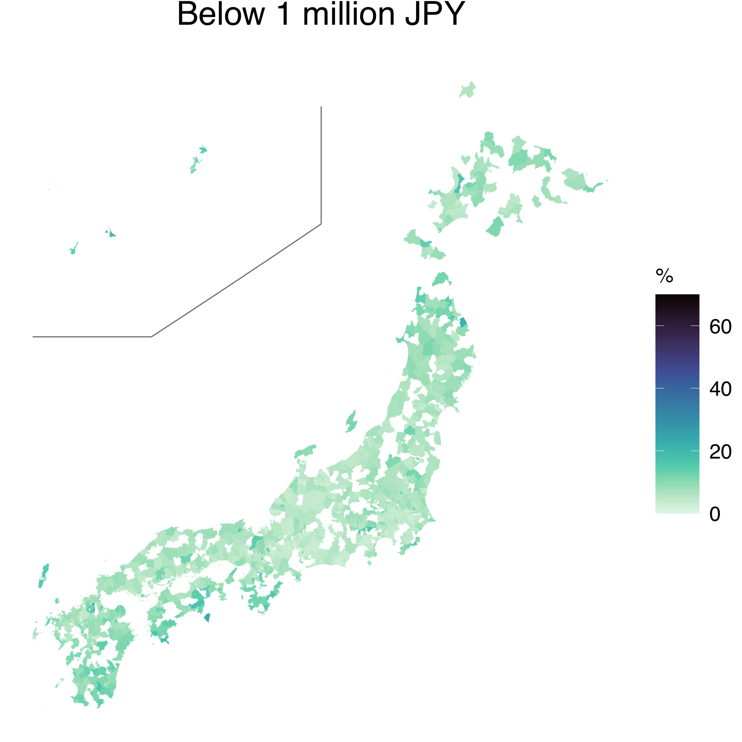
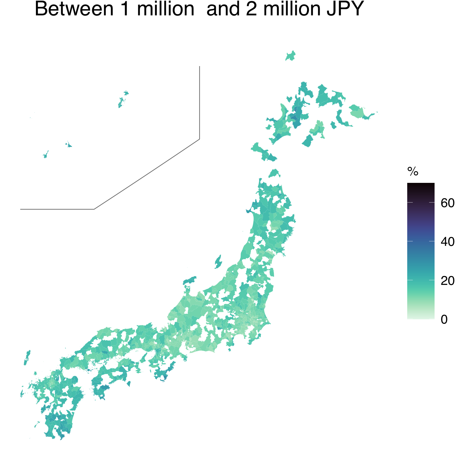
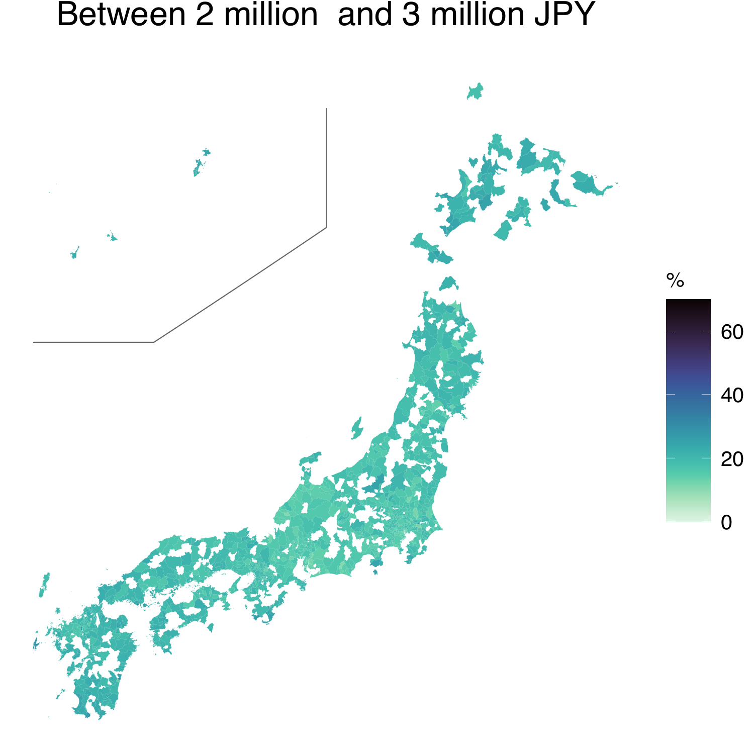
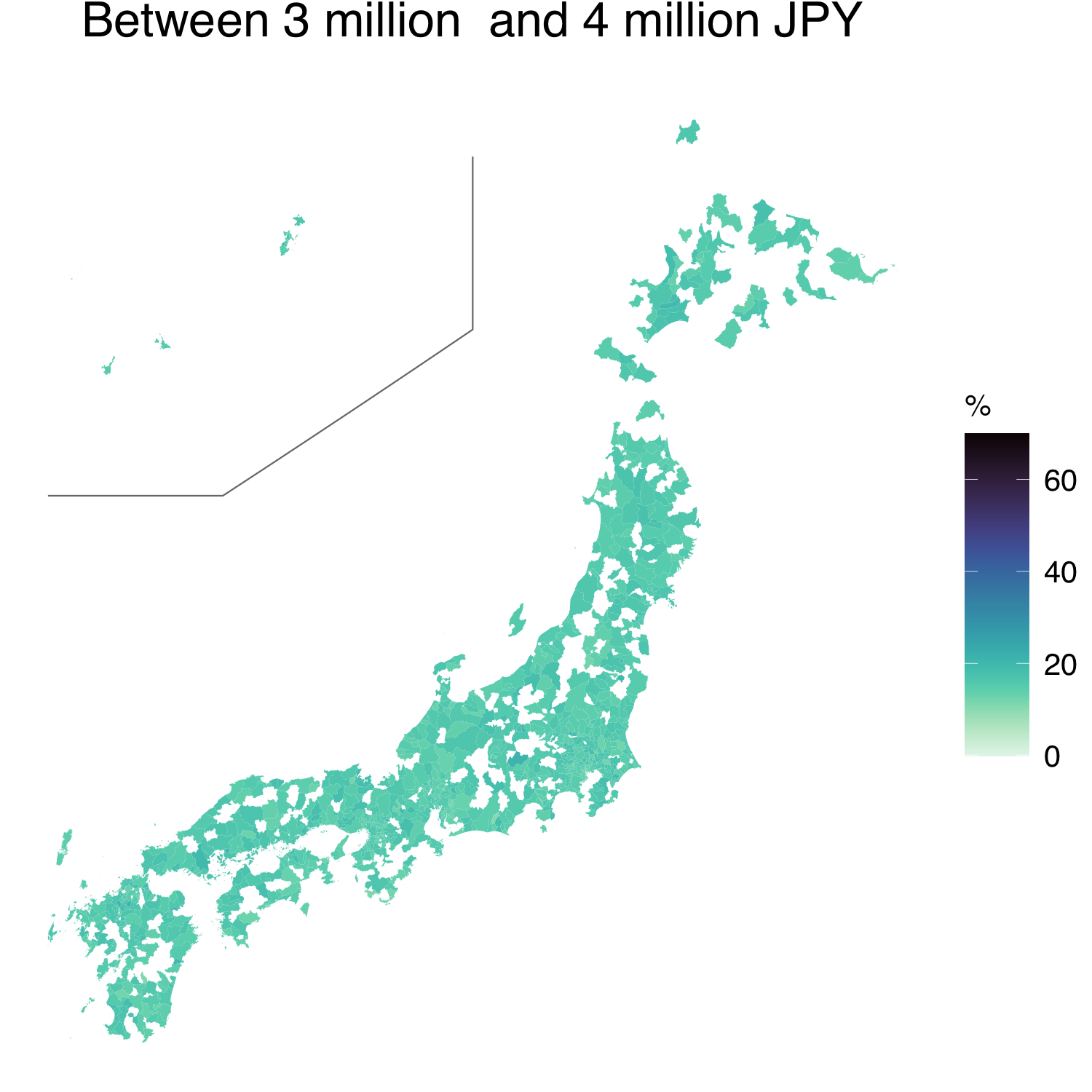
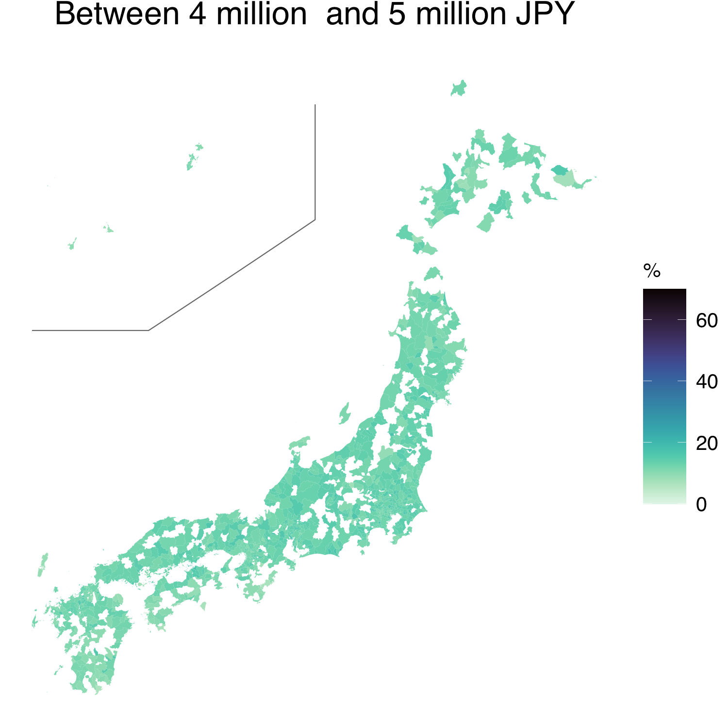
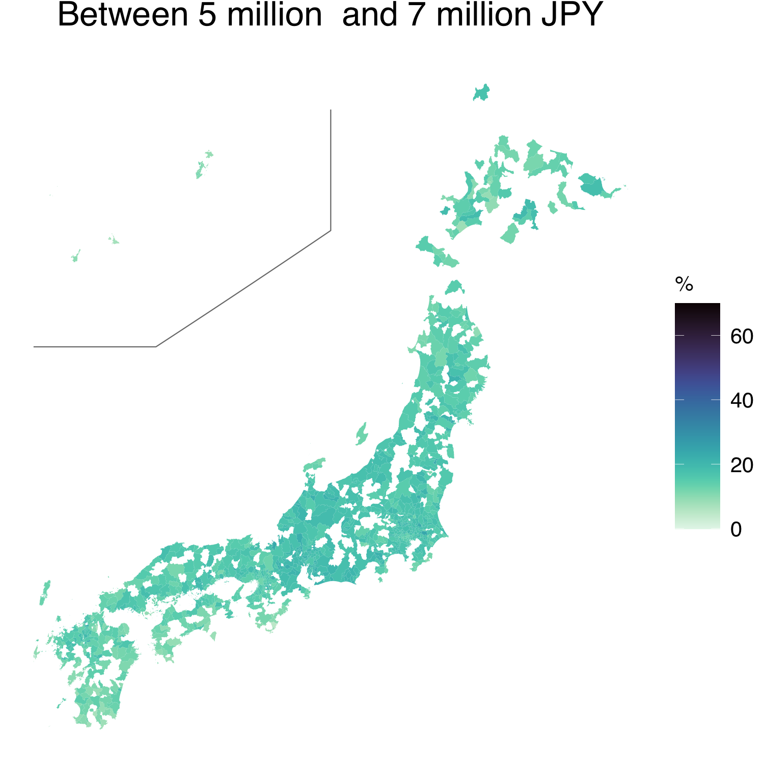
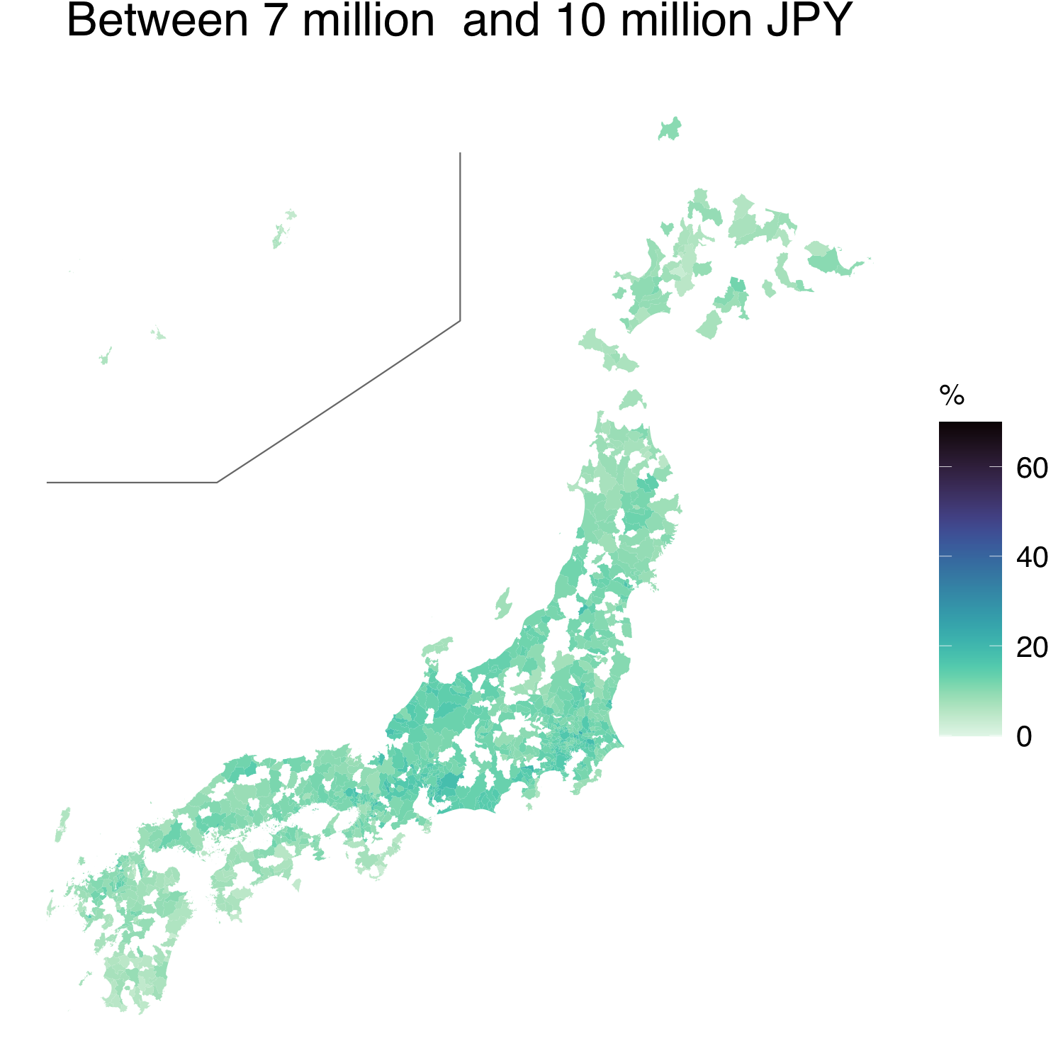
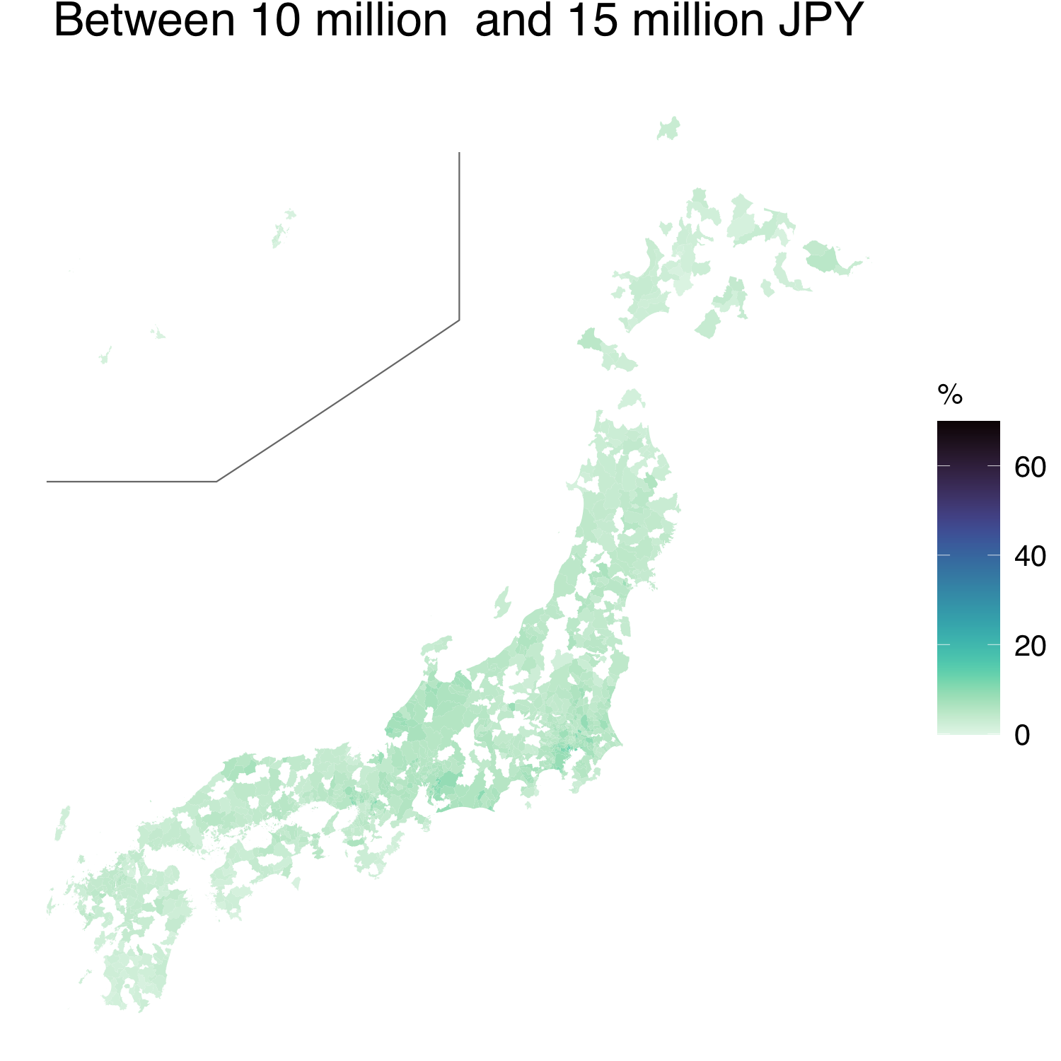
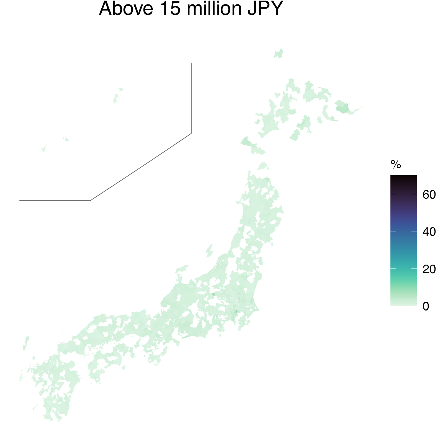
Figure 1: Proportions of the nine income classes in the 2018 HLS data.

Spatio-temporal mixture modelling

Model

Suppose that we are interested in the income distributions in $M$ areas over $T$ periods, denoted by $F_{it}(\cdot)$, with the density function, $f_{it}(\cdot)$, for $i=1,\dots,M$ and $t=1,\dots,T$. We also assume that the individual household incomes are not observed and that only the grouped data are available. Specifically, let $[Z_{t0},Z_{t1})$, $[Z_{t1},Z_{t2}),\dots,[Z_{t,G-1},Z_{tG})$ be $G$ income classes in the $t$th period, where $Z_{t0}$ and $Z_{tG}$ are typically set to $0$ and $\infty$, respectively. Thus, the number of households per interval is observed and denoted by $N_{itg}$, $g=1,\dots,G$. As is the case for the HLS data (see Section 5), we assume that all the $M$ areas are not sampled. Without a loss of generality, the first $m$ areas are sampled, and the remaining $m^{*}=M-m$ areas are not sampled for $t=1,\dots,T$. Further, the number of households in the $i$th area and $t$th period of the grouped data is denoted by $N_{it}=\sum_{g=1}^{G}N_{itg}$.

To model the underlying spatio-temporal income distributions flexibly, we consider a mixture of log-normal distributions, as follows:

$$f_{it}(y)=\sum_{k=1}^{K}\pi_{itk}\phi_{LN}(y;{\text{\boldmath$x$}}_{it}^{t}{\text{\boldmath$\beta$}}_{k},\sigma_{k}^{2}),\ \ \ \ i=1,\ldots,m,$$ (1)

where ${\text{\boldmath$x$}}_{it}=(1,x_{it1},\dots,x_{itp})^{t}$ is the $(p+1)$-dimensional vector of some external information correlated with the income data (e.g. the consumption or tax level), ${\text{\boldmath$\beta$}}_{k}=(\beta_{k0},\beta_{k1},\dots,\beta_{kp})^{t}$ and $\sigma_{k}^{2}$ are the coefficient and scale parameters of the $k$th component, respectively, and $\phi_{LN}(\cdot;\mu,\sigma^{2})$ denotes the density function of the log-normal distribution with the $\mu$ and $\sigma^{2}$ parameters.

The covariate, ${\text{\boldmath$x$}}_{it}$, in the component distribution in (1) is crucial. Regarding the spatial interpolation of the non-sampled municipalities, ${\text{\boldmath$x$}}_{it}$ must be observed for all the municipalities. Additionally, regarding the temporal prediction, it is also assumed that the most recent observations on ${\text{\boldmath$x$}}_{it^{*}}$ with $t^{*}>T$ become more frequently available than HLS, for example, annually. Our HLS data analysis is based on taxable income per taxpayer (see Section 5.1).

Employing only a log-normal distribution is known to fit income data very poorly. However, a mixture of log-normal distributions provides a good fit to data (Lubrano and Ndoye, 2016). Furthermore, (1) is merely assumed for the unobserved continuous household income. For the grouped income data, the likelihood contribution of the $i$th area in the $t$th period takes a multinomial form:

$$\prod_{g=1}^{G}\left\{F_{it}(Z_{tg})-F_{it}(Z_{t,g-1})\right\}^{N_{itg}},$$ (2)

for $i=1,\dots,m$ and $t=1,\dots,T$, where $F_{it}(y)=\sum_{k=1}^{K}\pi_{itk}\Phi_{LN}(y;{\text{\boldmath$x$}}_{it}^{t}{\text{\boldmath$\beta$}}_{k},\sigma^{2}_{k})$ is the distribution function of the $i$th area in the $t$th period, with the distribution function of the log-normal distribution, $\Phi_{LN}$.

The mixing proportion, $\pi_{itk}$, is modelled as

$$\pi_{itk}=\frac{\exp(\mu_{k}+u_{ik}+\eta_{tk})}{\sum_{\ell=1}^{K}\exp(\mu_{\ell}+u_{i\ell}+\eta_{t\ell})},\quad k=2,\ldots,K,$$ (3)

where $\mu_{k}$ determines the overall mixing proportion, $u_{ik}$ is the area-specific spatial effect, and $\eta_{tk}$ is the temporal effect. We denote the row-standardised adjacency matrix for all the $M$ areas as $W$. Employing $W$, we independently assume the simultaneous autoregressive (SAR) model for ${\text{\boldmath$u$}}_{{\rm all},k}=(u_{1k},\ldots,u_{Mk})^{t}$ for $k=2,\dots,K$. Namely, ${\text{\boldmath$u$}}_{{\rm all},k}\sim N({\text{\boldmath$0$}},\tau_{k}^{-1}{\text{\boldmath$Q$}}_{{\rm all},k}^{-1})$, where ${\text{\boldmath$Q$}}_{{\rm all},k}=\begin{pmatrix}{\text{\boldmath$Q$}}_{11k}&{\text{\boldmath$Q$}}_{12k}\\ {\text{\boldmath$Q$}}_{21k}&{\text{\boldmath$Q$}}_{22k}\end{pmatrix}=({\text{\boldmath$I$}}_{M}-\rho_{k}{\text{\boldmath$W$}})({\text{\boldmath$I$}}_{M}-\rho_{k}{\text{\boldmath$W$}})^{t}$, with the precision parameter, $\tau_{k}$, and correlation parameter, $\rho_{k}\in(0,1)$. The marginal distribution of the spatial effects for the sampled areas, ${\text{\boldmath$u$}}_{k}=(u_{1},\dots,u_{m})^{t}$, is $N({\text{\boldmath$0$}},\tau_{k}^{-1}{\text{\boldmath$Q$}}_{11k}^{-1})$. We assume that the temporal effect, $\eta_{tk}$, follows the random-walk process, $\eta_{tk}|\eta_{t-1,k}\sim N(\eta_{t-1,k},\alpha_{k})$, for $t=1,\dots,T$, where $\eta_{0k}$ is the initial location parameter.

Prior distributions

Here, we specify the prior distributions of the parameters. As these prior distributions are conditionally conjugate after data augmentation, they are convenient for the development of the Gibbs sampling algorithm. Regarding the parameters of the component distributions, $\beta_{k}$ and $\sigma_{k}^{2}$, we assume ${\text{\boldmath$\beta$}}_{k}\sim N({\text{\boldmath$0$}},c_{\beta}{\text{\boldmath$I$}}_{p})$ and $\sigma_{k}^{2}\sim IG(a_{\sigma},b_{\sigma})$ for $k=1,\dots,K$. As these component distributions, which are common over space and time, can be stably estimated, the default hyper-parameter choices are $c_{\beta}=100$ and $a_{\sigma}=b_{\sigma}=0.1$, such that they are diffuse. Regarding $\mu_{k}$, the normal prior, $\mu_{k}\sim N(0,c_{\mu}),k=2,\dots,K$, is assumed with the default value of $c_{\mu}=10$. By using the row-standardised adjacency matrix, the prior for the spatial-correlation parameter is given by $\rho_{k}\sim U(0,1),k=2,\dots,K$. For the precision parameter of the SAR model, $\tau_{k}$, we assumed $\tau_{k}\sim Ga(a_{\tau},b_{\tau}),k=2,\dots,K$ with the default $a_{\tau}=b_{\tau}=1$, such that it considerably covers the possible values. Regarding the initial location and variance of the random-walk process, we assume $\eta_{0k}\sim N(0,c_{\eta})$ and $\alpha_{k}\sim IG(a_{\alpha},b_{\alpha})$ for $k=2,\dots,K$. The default hyperparameters choices are $c_{\eta}=10$, $a_{\alpha}=3.0$, and $b_{\alpha}=1.0$.

Posterior inference

The posterior inference is based on the Markov chain Monte Carlo (MCMC) method. We develop a Gibbs sampling algorithm that is tuning-free as it does not require any Metropolis–Hastings (MH) steps. Although the details are presented in the Supplementary Material, we briefly describe the strategy for constructing the Gibbs sampler here. Firstly, to facilitate the sampling of the variables in $\pi_{itk}$, the Pólya-gamma data augmentation of Polson et al. (2013) is employed so that these variables can be sampled from the normal distributions. Second, we introduce a latent variable, which indicates the number of households in the $g$th income class belonging to the $k$th component of the mixture. Third, the latent individual household incomes are introduced to easily sample ${\text{\boldmath$\beta$}}_{k}$ and $\sigma^{2}_{k}$. Conditionally on the data and number of households in the $g$th income class and $k$th mixture component, the logarithms of individual household incomes are generated from the truncated normal distributions. Finally, ${\text{\boldmath$\beta$}}_{k}$ and $\sigma_{k}^{2}$ are sampled from their full conditional distributions, which from conditional conjugacy are the normal and inverse gamma, respectively.

Based on the MCMC output, the posterior inference of the quantities of interest can be obtained. In this context, we are interested in the average income, ${\rm AI}_{it}=\sum_{k=1}^{K}\pi_{itk}\exp({\text{\boldmath$x$}}_{it}^{t}{\text{\boldmath$\beta$}}_{k}+\sigma_{k}^{2}/2)$, median income, and Gini index for $i=1,\dots,M$ and $t=1,\dots,T$. Under the mixture model, the median income and Gini index cannot be obtained analytically. Regarding the median income, $\sum_{k=1}^{K}\pi_{itk}\Phi_{LN}(\text{MI}_{it};{\text{\boldmath$x$}}_{it}^{t}{\text{\boldmath$\beta$}}_{k},\sigma_{k}^{2})=0.5$ is solved numerically for ${\rm MI}_{it}$. For the Gini index, which is defined by ${\rm Gini}_{it}={\rm AI}_{it}^{-1}\int_{0}^{\infty}F_{it}(z)(1-F_{it}(z))dz$, the integral is numerically evaluated, following Lubrano and Ndoye (2016).

To interpolate the non-sampled areas, given the MCMC draws of the parameters and latent variables, ${\text{\boldmath$u$}}^{*}_{k}=(u_{m+1,k},\dots,u_{Mk})^{t}$ is sampled from the conditional distribution of the SAR model: $N(\mu_{k}{\text{\boldmath$\iota$}}_{m^{*}}-{\text{\boldmath$Q$}}_{22k}^{-1}{\text{\boldmath$Q$}}_{21k}({\text{\boldmath$u$}}_{k}-\mu_{k}{\text{\boldmath$\iota$}}_{m^{*}}),\tau_{k}^{-1}{\text{\boldmath$Q$}}_{22k}^{-1})$. Regarding the temporal prediction, $\eta_{T+1,k}$ is drawn from $N(\eta_{Tk},\alpha_{k})$.

In practice, the number of components, $K$, is unknown. However, it affects the estimation performance or interpretation of the estimation results. Following Celeux (1999), Fürwirth-Schnatter and Pyne (2010), and Malsiner-Walli et al. (2016), $k$-means clustering is applied to the MCMC output of ${\text{\boldmath$\beta$}}_{k}$. Suppose we have $S$ MCMC draws of $\beta_{k}$, denoted by ${\text{\boldmath$\beta$}}_{k}^{(s)}$, for $s=1,\dots,S$ and $k=1,\dots,K$. Then, $S\times K$ ${\text{\boldmath$\beta$}}_{k}^{(s)}$’s are used as the input for $k$-means clustering that assigns the label, $r_{k}^{(s)}=r({\text{\boldmath$\beta$}}_{k}^{(s)})\in\left\{1,\dots,K\right\}$, to each ${\text{\boldmath$\beta$}}_{k}^{(s)}$ for $s=1,\dots,S$ and $k=1,\dots,K$. The fraction of MCMC draws whose cluster labels of the $k$-means match the permutation of $(1,\dots,K)$ is computed. In practice, the matching fraction is computed as $S^{-1}\sum_{s=1}^{S}I\left\{\sum_{k=1}^{K}r_{k}^{(s)}=K(K+1)/2\right\}$, where $I\left\{\cdot\right\}$ denotes the indicator function. For example, when $K$ clusters are well-separated and $\{r_{1}^{(s)},\ldots,r_{K}^{(s)}\}$ is equivalent to $\{1,\ldots,K\}$ as a set, $\sum_{k=1}^{K}r_{k}^{(s)}=K(K+1)/2$ is satisfied. If a matching fraction of the MCMC draws for a given $K$ is less than one, it indicates the over-fitting of the mixture; thus, a smaller $K$ is preferred.

Simulation study

The proposed method is first demonstrated using simulated data. The $M=200$ areal units on the two-dimensional space are generated by sampling each coordinate from $(d_{i1},d_{i2})\sim U(-1,1)^{2}$. The neighbours of an area are defined as those with coordinates within a $0.2$ Euclidean distance, and the average number of neighbours is $5.77$. In each area, $N_{it}$ is generated from $U(100,500)$ for $21$ periods. The groups are represented by $[0,1)$, $[1,2)$, $[2,3)$, $[3,4)$, $[4,5)$, $[5,7)$, $[7,10)$, $[10,15)$, and $[15,\infty)$ with $G=9$ for all $t$. These corresponded to those in the latter three HLS rounds (Table 1). In this simulation study, the grouped data are generated from the mixture model, (1), with $K=3$. The parameters of the component distribution are set, as follows: ${\text{\boldmath$\beta$}}_{1}=(0.5,0,1)^{t}$, ${\text{\boldmath$\beta$}}_{2}=(-0.5,1,0)^{t}$, ${\text{\boldmath$\beta$}}_{3}=(2.0,-1,-1)^{t}$, $(\sigma^{2}_{1},\sigma_{2}^{2},\sigma_{3}^{2})=(0.5,0.5,0.5)$. Each covariate, $x_{itj}$, is generated from the uniform distribution.

Using the same component distributions, the following two settings for the mixing proportions are considered. In the first setting, the mixing proportions are generated from (3) with $(\mu_{2},\mu_{3})=(-0.2,0.1)$, $(\rho_{2},\rho_{3})=(0.8,0.8)$, $(\tau_{2},\tau_{3})=(0.1,0.1)$, $(\alpha_{2},\alpha_{3})=(0.2,0.2)$, $(\eta_{02},\eta_{03})=(0,0)$. In the second setting, the spatial and temporal effects are determined by the following deterministic sequences: $u_{i2}=3(d_{i1}-d_{i2})$, $u_{i3}=3(d_{i2}-d_{i1})$, $\eta_{t2}=t/3-(T+1)/6$, $\eta_{t3}=t/6-T/12$. Furthermore, the two-dimensional space, $(-1,1)^{2}$, is partitioned into $5\times 5$ square blocks. The areas in the same block exert the same effect on the mixing proportions: $a_{h_{i}k}\sim N(0,0.2^{2}),\ h_{i}\in\{1,\dots,25\},\ i=1,\dots,200,\ k=2,3$. In this setting, the area, $i$, is a sub-area of the $h_{i}$th block. Thus, the mixing proportions for the $i$th area corresponded to the $h_{i}$th block are proportional to $\exp(\mu_{k}+u_{ik}+\eta_{tk}+a_{h_{i}k})$ for $k=2,3$. The average number of sub-areas in each block is $8$.

First, we fit the proposed spatio-temporal mixture model described in Section 3 with different component numbers: $K=2,\dots,6$. The proposed Gibbs sampler is run for 20,000 iterations, with an initial burn-in period of 10,000 iterations. Figure 2 shows the matching fractions for the proposed mixture models under both settings. The matching fractions are one as long as $K\leq 3$ in both settings. However, the figure shows that the matching fractions become less than one for the over-specified models with $K=4$, $5$, and $6$, indicating the overfitting of the mixture models. The figure indicates that the monitoring of the matching fraction from a small value of $K$ and the selection of an appropriate $K$ at the kink are reasonable approaches.

Figure 2: Fractions of the MCMC draws whose the outputs from the $k$-means clustering match the permutation of $(1,\dots,K)$.

Next, we compare the proposed spatio-temporal mixture model with four alternative models. The first alternative model is the mixture model based on (1) and (3). The mixing proportions are modelled with the two-way independent random effects that represent the heterogeneity in space and time: $u_{ik}\sim N(0,\tau_{k})$, $\eta_{tk}\sim N(0,\alpha_{k})$, respectively. As this model exerts spatial and temporal effects, it can be used for spatial interpolation and temporal prediction. The second alternative model is the mixture of the log-normal distributions with the mixing proportions that include only $\mu_{k}$ and $u_{ik}$. It is a purely spatial model, which is independently fitted for each $t$ and used for spatial interpolation only. This model may be considered as a spatial mixture extension of the small area model for grouped data proposed by Kawakubo and Kobayashi (2023). The third alternative is the simple log-normal model for grouped data. It is independently estimated using the maximum likelihood for each area and period. The fourth alternative is an SAE model. More specifically, we consider the linear mixed model proposed by Torabi and Rao (2014), as recommended by one of the reviewers. It is given by the following:

$$\hat{y}_{bj}={\text{\boldmath$x$}}^{t}_{bj}{\text{\boldmath$\beta$}}+v_{b}+u_{bj}+e_{bj},\quad b=1,\dots,25,\quad j=1,\dots,M_{b},$$

where $M_{b}$ is the number of sub-areas in the area, $b$, such that $\sum_{b=1}^{25}M_{b}=200$, $\hat{y}_{bj}$ is the crude average income described below, $v_{b}\sim N(0,\sigma^{2}_{v})$ is the area effect, $u_{bj}\sim N(0,\sigma^{2}_{u})$ is the sub-area effect, and $e_{bj}\sim N(0,\sigma^{2}_{ej})$ is the sampling error. The average incomes are computed based on $N_{it}^{-1}\sum_{g=1}^{G}N_{itg}{\rm mid}_{tg}$, where ${\rm mid}_{tg}$ is the mid-point of the income classes. For the top-income class ($g=G$) with an open-ended interval, ${\rm mid}_{tG}$ is set to be $20$. This model is fitted in Setting 2, whereas the model without $v_{b}$ is fitted in Setting 1 as the true model does not have a sub-area structure. The small area models are estimated independently per period.

The data for the $m=150$ areas and $T=20$ periods are used for model estimation. The data for the remaining $m^{*}=50$ areas and the last period are subjected to spatial interpolation and temporal prediction.

The models are first compared based on the root mean squared errors (RMSE) and coverage of the 95% credible or prediction intervals for the average incomes in the in-sample estimation, spatial interpolation, and temporal prediction. For example, in the in-sample estimation case, RMSE is defined by $\sqrt{\frac{1}{mT}\sum_{i=1}^{m}\sum_{t=1}^{T}(\widehat{\rm AI}_{it}-{\rm AI}_{it})^{2}}$, and the coverage is defined by $\frac{1}{mT}\sum_{i=1}^{m}\sum_{t=1}^{T}I\left\{L_{it}\leq\text{AI}_{it}\leq U_{it}\right\}$, where ${\rm AI}_{it}$ is the truth, $\widehat{\rm AI}_{it}$ is the posterior mean or maximum likelihood estimate for the sampled areas and $L_{it}$ and $U_{it}$ are the endpoints of the 95% credible interval under the Bayesian models. Regarding the spatial interpolation and temporal prediction cases, $\widehat{\rm AI}_{it}$ corresponds to the posterior predictive mean for the non-sampled areas with $i=m+1,\dots,M$ and $t=1,\dots,T$; it also corresponds to the posterior predictive mean for all the areas with $t=T+1$. Similarly, $L_{it}$ and $U_{it}$ correspond to the endpoints of the 95% prediction intervals.

Table 2 presents the RMSEs and coverages for the average incomes under the five models. Generally, the proposed model outperform the other models regarding the RMSE. The coverages are around the targeted value of $0.95$. Regarding the two-way model, although the RMSEs in the in-sample estimation are the second smallest in both settings, following the proposed model, it produced high RMSEs in the spatial interpolation and temporal prediction. In addition, the coverages are lower than the target value of $0.95$. The RMSEs of the spatial model regarding the spatial interpolation are the second smallest in both settings, following the proposed model, with the coverages of approximately $0.95$. The results indicate the efficacy of the spatio-temporal effects, and the proposed model comprising both effects demonstrated superior performance. Estimating the grouped-data model for each area and period separately via maximum likelihood resulted in high RMSEs in the in-sample estimation because of the lack of borrowing information across space and time. The employed SAE method is not designed specifically for grouped data or a spatio-temporal setting. Thus, it produced the largest RMSEs for the in-sample estimation and spatial interpolation.

Finally, the proposed, two-way, and spatial models are compared based on the RMSE and coverage for the number of households. Table 3 presents the results for both settings. The proposed model with the spatial and temporal effects performs well, exhibiting the smallest RMSEs, except for the in-sample estimation in Setting 2 and the coverages around the targeted $0.95$. The two-way model yielded the largest RMSEs in all cases. The spatial model produced smaller RMSEs than the two-way model regarding the spatial interpolation. However, the proposed model that borrows information over time produced smaller RMSEs than those of the spatial model.

Table 2: RMSEs and coverages of the average incomes in the in-sample estimation, spatial interpolation for the non-sampled areas, and temporal prediction using the proposed spatio-temporal (Proposed), two-way independent spatio-temporal (Two-way), separate spatial (Spatial), SAE, and separate grouped maximum likelihood (GML) approaches.

			Proposed	Two-way	Spatial	SAE	GML
Setting 1	RMSE	In-sample	0.035	0.085	0.185	0.345	0.217
		Spatial	1.094	1.400	1.188	1.420	—
		Temporal	0.493	0.597	—	—	—
	Coverage	In-sample	0.952	0.553	0.992	0.929	—
		Spatial	0.976	0.810	0.953	0.888	—
		Temporal	0.990	0.910	—	—	—
Setting 2	RMSE	In-sample	0.048	0.049	0.131	0.417	0.254
		Spatial	0.375	1.032	0.471	0.762	—
		Temporal	0.254	0.875	—	—	—
	Coverage	In-sample	0.920	0.908	0.947	0.958	—
		Spatial	0.985	0.862	0.978	0.874	—
		Temporal	0.975	0.875	—	—	—

Table 3: RMSEs and coverages for the numbers of households in the in-sample estimation, spatial interpolation for the non-sampled areas, and temporal prediction under the proposed spatio-temporal (Proposed), two-way spatio-temporal (Two-way), and separate spatial (Spatial) models

			Proposed	Two-way	Spatial
Setting 1	RMSE	In-sample	5.027	5.264	5.229
		Spatial	20.446	25.184	21.552
		Temporal	6.721	8.059	—
	Coverage	In-sample	0.968	0.959	0.970
		Spatial	0.963	0.906	0.951
		Temporal	0.973	0.964	—
Setting 2	RMSE	In-sample	5.065	5.074	4.681
		Spatial	7.798	18.382	9.130
		Temporal	5.104	11.721	—
	Coverage	In-sample	0.968	0.968	0.981
		Spatial	0.977	0.938	0.980
		Temporal	0.979	0.962	—

Analysis of the HLS data

Set-up

In our analysis, we use the HLS data of the total annual household incomes, including salary and transfer incomes, of general households. We use the data from 800 municipalities for the model estimation, of which observations are available in all the rounds. The remaining observations are held out to compare the performance of the models (Section 5.2). As the data span over 20 years, the endpoints of the income classes (Table 1) are adjusted based on the consumer price index using 2018 as the standard. Thereafter, a temporal comparison of the income distributions can be made.

Regarding the covariate, we employ the taxable income per taxpayer in millions JPY, denoted by $\text{tax}_{it}$, and set ${\text{\boldmath$x$}}_{it}=(1,\text{tax}_{it},\text{tax}_{it}^{2})^{t}$. This covariate is obtained from the tax survey data of the Ministry of Internal Affairs and Communications of Japan. These data are available annually for all municipalities in Japan and can reasonably predict the income based on HLS. As in the case of income classes, the taxable incomes are adjusted based on the consumer price index. The spatial distributions of the taxable incomes per taxpayer are presented in Supplementary Material.

Notably, although this auxiliary information is available annually at the municipality level, it cannot be used independently to infer income distributions. However, this vital information must be incorporated as a covariate in our proposed model for accurate spatial interpolation and temporal prediction.

Model comparison

The proposed Gibbs sampler is run for 30,000 iterations, with an initial burn-in period of 10,000 iterations. Figure 3 shows the fractions of the MCMC draws whose outputs from the $k$-means clustering match the permutation of $(1,\dots,K)$ for different numbers of mixture components between 2 and 8. The matching fractions are one for $K\leq 4$ under the proposed model. Regarding $K>4$, the matching fractions are below one, indicating overfitting. Figure 3 shows the results of the model with the two-way independent effects; we observe a similar pattern to that of the proposed model.

The numbers of households in the income groups of the holdout municipalities are predicted using spatial interpolation. The proposed model is compared with the two-way and parametric spatial income models for grouped data proposed by Sugasawa et al. (2020). In the model of Sugasawa et al. (2020), the parameters of the parametric income distribution vary over space through the appropriate transformation of the spatial random effects. We consider the Singh-Maddala and Dagum distributions as the parametric models as they are frequently used in income modelling (Kleiber and Kotz, 2003). The performances of the four models are compared based on the coverage of the 95% prediction interval, as well as the $0.5$, $0.9$th, and $0.99$th quantiles of the relative absolute error (RAE) for the number of households defined by $|\hat{N}_{itg}-N_{itg}|/(N_{itg}+1)$, where $\hat{N}_{itg}$ denotes the posterior predictive mean for the holdout municipality. Table 4 reveals that the proposed and two-way models produced the desired coverage of approximately $0.95$. The Singh-Maddala and, especially the Dagum models, resulted in undercoverage. Although the proposed and Dagum models produced the comparable median RAEs, the $0.9$th and $0.99$th quantiles of RAE under the Dagum model are larger than those under the proposed model. The Singh-Maddala model produced the largest RAE quantiles. Overall, the table reveals that the proposed model exhibited the best performance.

Based on the observations in Figure 3 and Table 4, in the following analysis, we adopt $K=4$ for the proposed spatio-temporal mixture model in the subsequent analysis. The posterior distributions of the parameters for $K=4$ are presented in Supplementary Material.

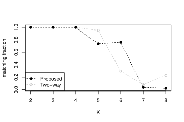
Figure 3: Matching fractions of the MCMC draws whose outputs from the $k$-means clustering match the permutation of $(1,\dots,K)$ for the HLS data.

Table 4: Coverages, as well as 0.5th, 0.9th, and 0.99th quantiles of RAEs for the holdout municipalities under the proposed spatio-temporal model (Proposed), two-way spatio-temporal model (Two-way), and Dagum and Sing-Maddala models

		Quantiles of RAE
Model	Coverage	$0.5$th	$0.9$th	$0.99$th
Proposed	0.955	0.136	0.411	1.105
Two-way	0.950	0.161	0.469	1.259
Dagum	0.553	0.130	0.445	1.383
Singh-Maddala	0.869	0.196	0.875	3.654

Income maps of Japan

We present the complete income maps of Japan for the HLS years, as well as 2020 during which HLS was not conducted. In the survey years, the non-sampled municipalities are subjected to spatial interpolation. In 2020, all the municipalities are subjected to temporal prediction. The temporal effect for 2020 is generated from $N(\eta_{Tk},\frac{2}{5}\alpha_{k})$ as an increment in $t$ corresponds to a five-year increment.

Figure 4 shows the complete maps of the average incomes of Japan. The municipalities with darker colours indicate areas with higher incomes. The overall shades of the maps tend to become lighter with time. For example, the municipalities in the middle of the main island (Honshu) exhibit a much darker colour than those on the western islands (Shikoku and Kyushu). However, in 2018, the municipalities with high incomes are mostly concentrated in the metropolitan areas only. In 2020, the predicted average incomes exhibit similar patterns to those in 2018. We also observe a similar pattern in the median incomes; the results are presented in Supplementary Material.

Figure 5 shows the posterior and posterior predictive means of the Gini indices. The darker colours indicate the municipalities with relatively high Gini indices. The variation in the Gini indices across the country may have shrunken over the 20 years. For example, in 1998, the municipalities in the northern and, especially south western parts of Japan, are represented by dark colours, whereas those in the middle part of the main island are represented by light colours. The figure shows that the Gini indices were high throughout Japan in 2003. However, in 2018, although the municipalities in the western and northern parts of Japan still exhibit relatively high Gini indices, the overall shade of the map appears to be more uniform.

Figure 6 presents the changes in the distributions of the average incomes, median incomes, and Gini indices across Japan between 1998 and 2020. Th overall average and median incomes exhibit clear decreasing trends. The figure also reveals that the variation in the Gini indices decreased with time.

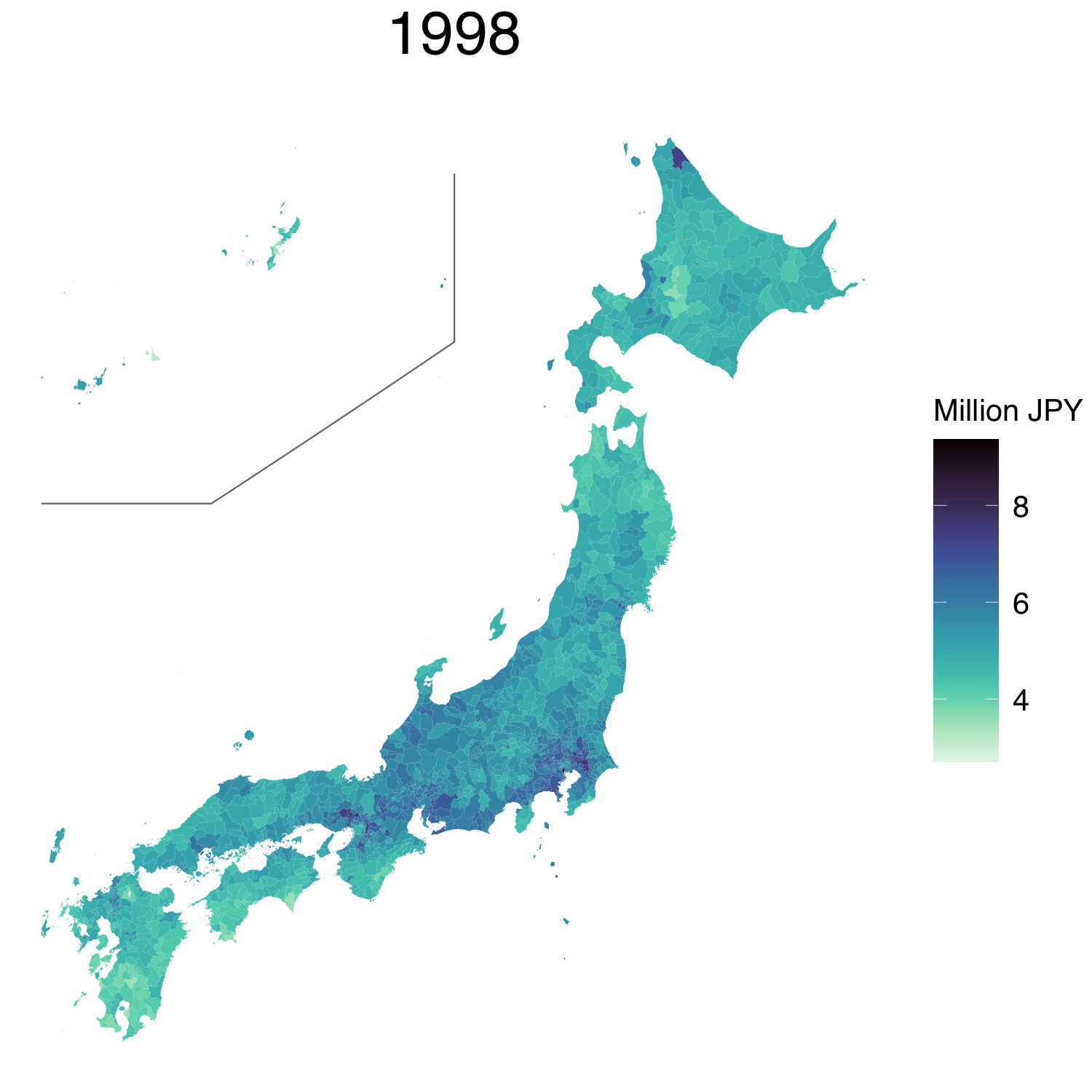
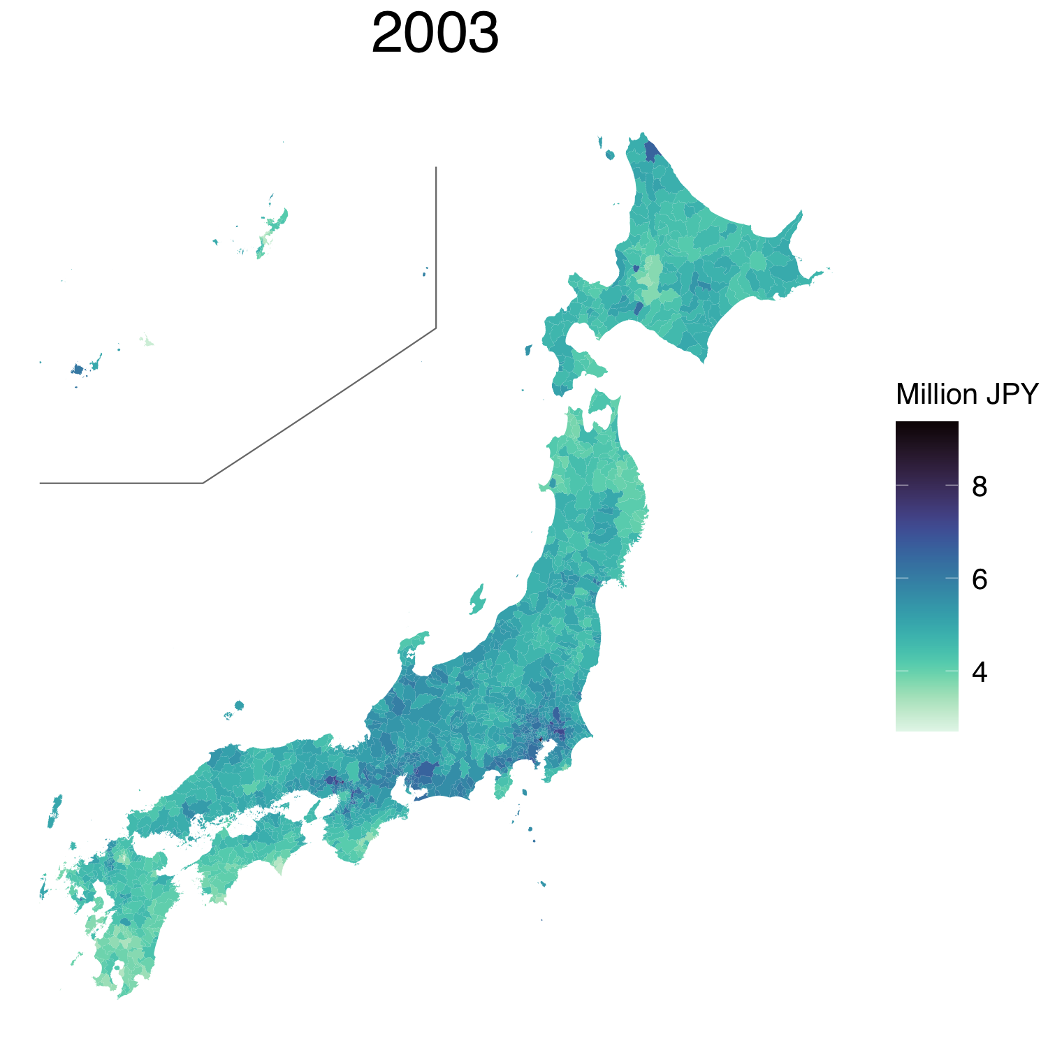
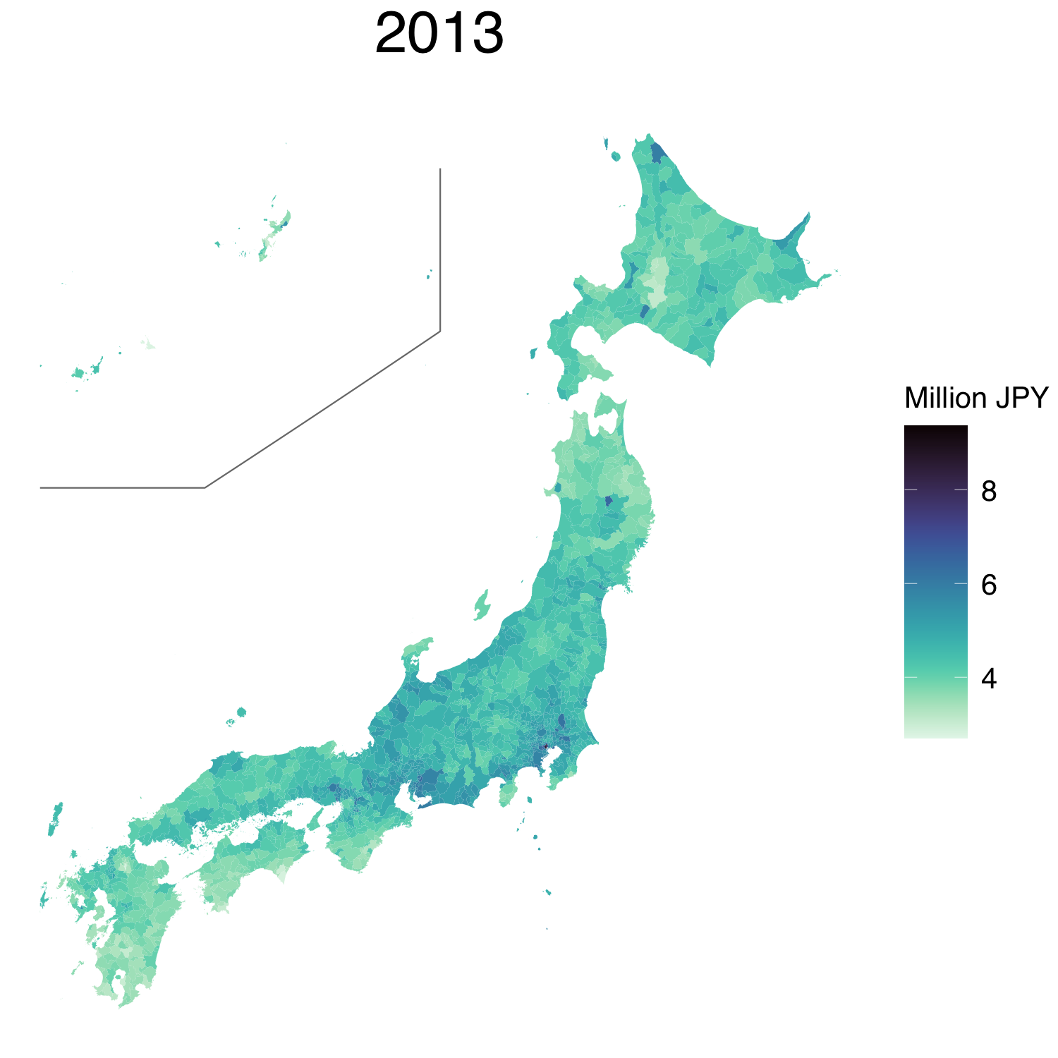
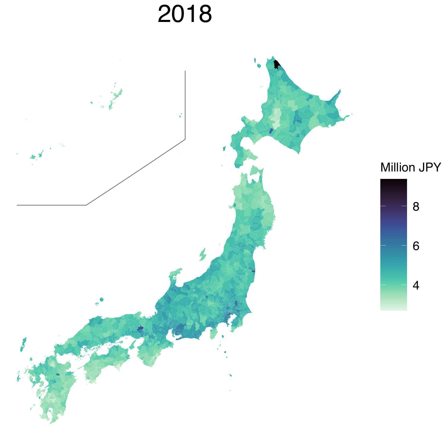
Figure 4: Completed maps of the average incomes

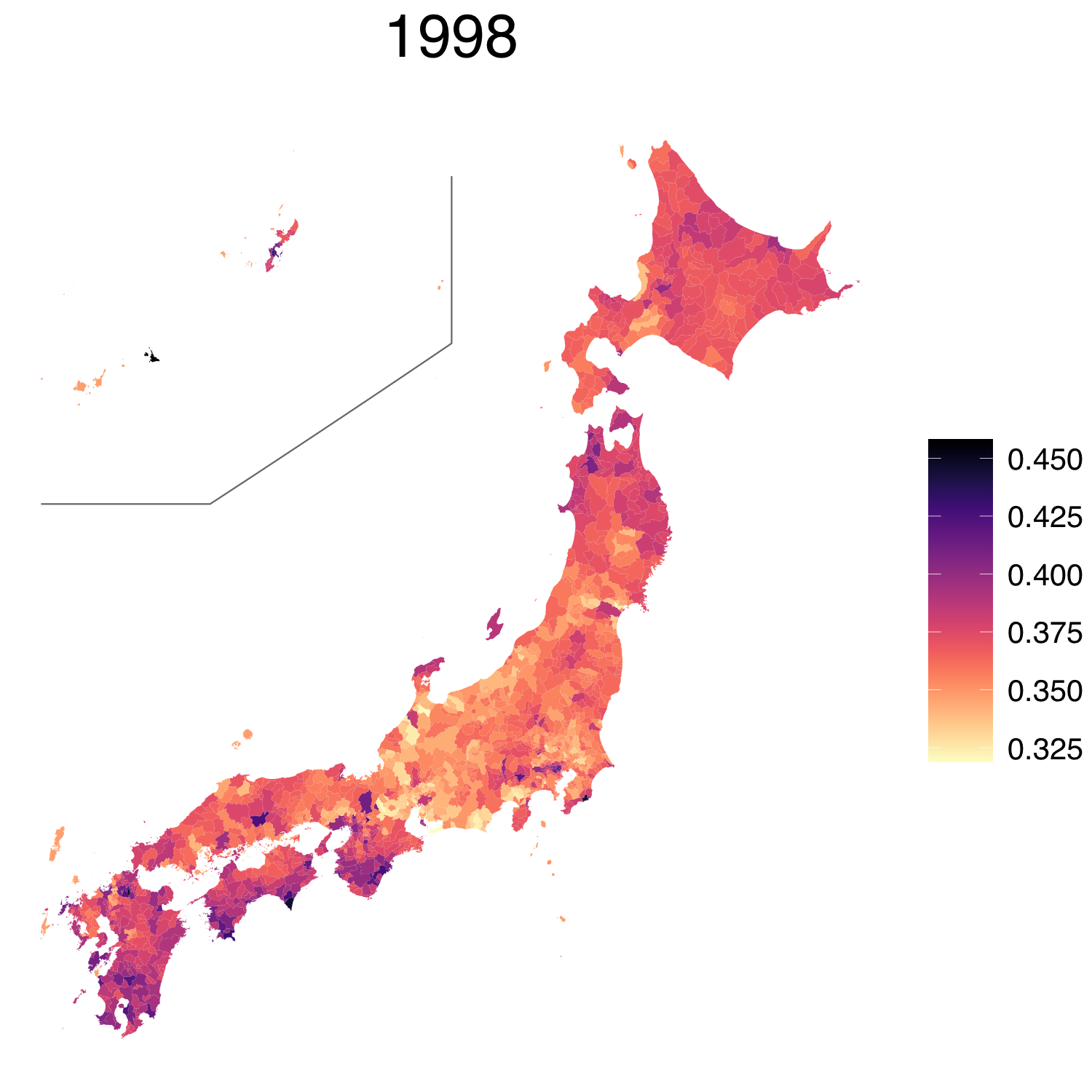
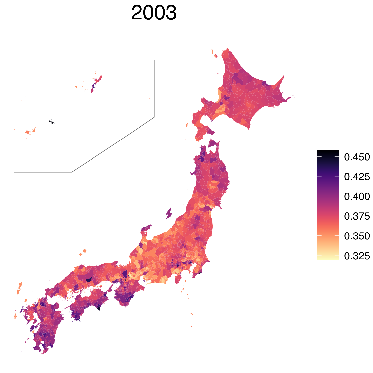
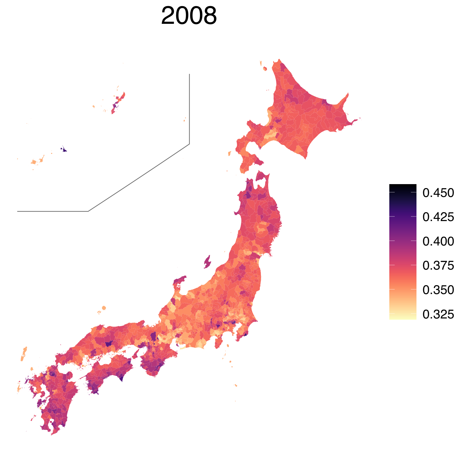
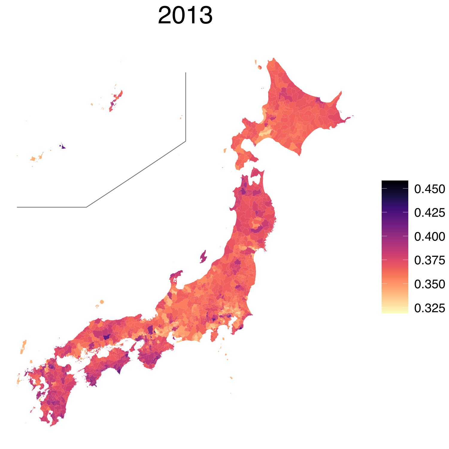
Figure 5: Completed maps of the Gini indices

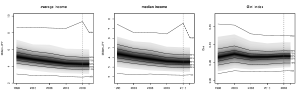
Figure 6: Changes in the distributions of the average incomes, median incomes, and Gini indices with time. The vertical line indicates that the last HLS was conducted in 2018

Area-wise income distributions

Here, we focus on the area-wise income distributions of the eight arbitrarily selected municipalities. The locations of the selected municipalities are shown in Figure 7. The sampled and non-sampled municipalities are represented by blue and red, respectively.

Figure 8 shows the posterior means of the income distributions in the survey years and 2020 when there was no survey. The top and bottom rows correspond to the sampled and non-sampled municipalities, respectively. The various income distribution shapes are obtained through the proposed mixture model over space and time. For example, Minato, one of the wealthiest parts of Tokyo, exhibits a long right tail compared with other municipalities. Contrarily, Ninohe, Satsuma, and Nakatosa in the far northern part of Honshu, the far western part of Honshu, and southern Shikoku exhibit short right tails, respectively. The bodies of these distributions are well concentrated below the 10 million Yen of annual income.

Interestingly, the income distributions of Oshino display the long right tail, which is similar to that of Minato. Oshino is a small town and was not sampled in HLS. However, it is also home to the headquarter and factories of a major electric machinery manufacturer and would account for a high-income level. The results demonstrate that the proposed model can infer the income distribution of such an area through the auxiliary information that is included as covariates and spatio-temporal mixing proportions. In all the municipalities listed in the figure, except for Oshino, the right tails of the income distributions became shorter slightly, and the densities of the distributions in the low-income regions increased over the past 20 years.

Figure 9 shows the posterior and posterior predictive means of the average incomes, median incomes, and Gini indices of the selected areas with time. The figure shows that the average and median incomes of all the municipalities, except Oshino, decreased with time. The Gini index of Minato is approximately $0.41$ over time, and that of Oshino increased gradually from $0.38$ to approximately $0.4$. Regarding the remaining areas, the variation in the Gini indices decreased over the past 20 years, similar to the nationwide result.

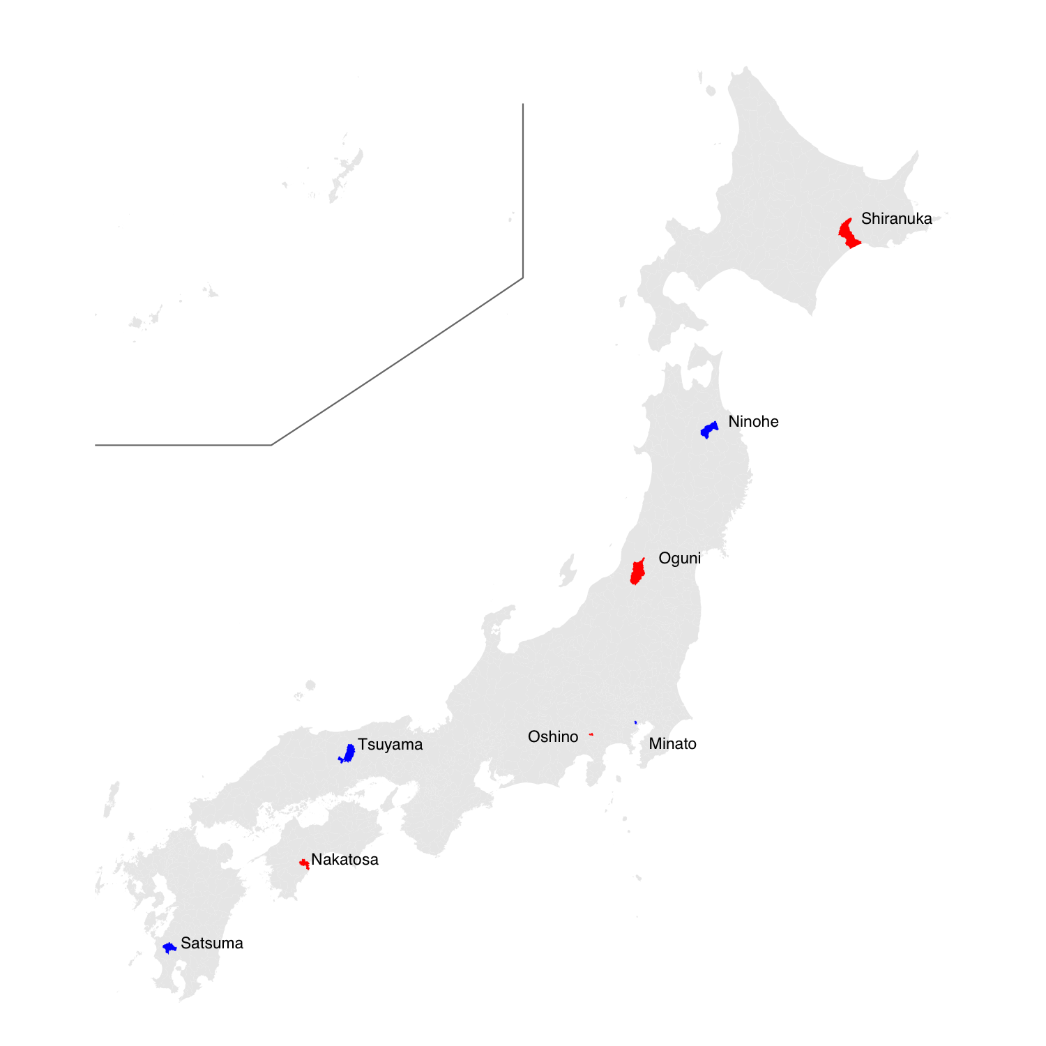
Figure 7: Locations of the arbitrarily selected municipalities (blue: sampled, red: non-sampled)

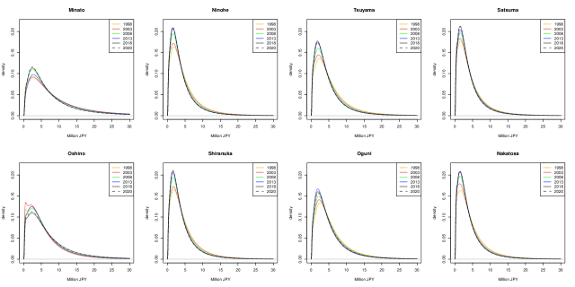
Figure 8: Posterior and posterior predictive means of the income distributions of the selected sampled (top row) and non-sampled (bottom row) municipalities with time

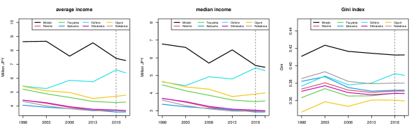
Figure 9: Average incomes, median incomes and Gini indices for the selected areas with time. The vertical dashed lines indicate that the last HLS was conducted in the year 2018

Prior sensitivity check

Finally, the sensitivity regarding the prior specification for the scale parameters is assessed. Figure 10 presents the scatterplots of the posterior means of the average incomes, median incomes, and Gini indices under the default inverse gamma and alternative priors. In the alternative prior setting, the standard deviations, $\sigma_{k}$ and $\sqrt{\alpha}_{k}$, follow the exponential distributions with a mean, $0.2$, which favours a smaller standard deviation, with the prior probability of a standard deviation exceeding $0.5$, which is approximately $0.08$. The figure shows that these posterior quantities of interest are robust regarding the prior specifications. Supplementary Material provides a comparison of the posterior distributions of the standard deviation parameters under those prior settings.

Figure 10: Scatterplots of the posterior means of the average incomes, median incomes, and Gini indices under the default inverse gamma (IG) and alternative exponential (Exp) priors.

Discussion

In this study, we proposed a novel spatio-temporal mixture model for analysing income distribution based on grouped data. Through the covariate information and spatio-temporal heterogeneous effects, the proposed model allows for the inference and prediction of the income distributions of sampled and non-sampled areas at any time point. When an appropriate covariate is available at a higher frequency than the grouped income data, a great insight into the latest income status can be obtained through predictions. By applying the proposed method to the HLS data, we obtained the complete maps of the average incomes, median incomes, and Gini indices. We observed that the overall average and median incomes decreased over the past 20 years and that the variation in the Gini indices decreased over the same period. We also demonstrated that adopting an appropriate covariate was essential to revealing the income statuses of the areas. This is particularly true for the non-sampled areas, where the covariate information is the only available information that can be used to infer income statuses.

The proposed method can reveal the income distributions and associated poverty measures of any area and at any period as long as their covariate information is available. While it was not shown in the present paper, it is also possible to estimate the proportions of the population in each area whose incomes are below any given threshold income levels. Exploring the results of the proposed method, policymakers can identify areas that require political intervention to mitigate poverty and inequality across the nation through efficient policy implementation and resource allocation. Such political interventions can be implemented based on the latest information on income distributions, as elucidated by the spatial interpolation and temporal prediction of the proposed model.

This study adopts the full MCMC approach to the posterior inferences. The advantage of the proposed Gibbs sampler is its non-requirement of algorithm tuning. As the inclusion of many latent variables may cause some inefficiencies, we may argue for the need for an alternative computational strategy. In fact, we also attempted to implement an MH algorithm and its adaptive version to sample ${\text{\boldmath$\beta$}}_{k}$ and $\sigma^{2}_{k}$ without generating individual household incomes. Put differently, (2) was directly used to contribute to the likelihood function. However, the MH algorithms failed to explore the parameter space and mostly stuck around the initial values. Some other faster posterior-computing methods, such as the integrated nested Laplace approximation (Rue et al., 2009) and the variational Bayes approximation (Blei et al., 2017), are appealing alternatives. Regarding the application to the HLS data, the computing time, e.g. for $K=4$ was approximately 40 hours based on non-optimised R code on the Apple M1 Ultra chip without any parallelisation. As we prefer to ensure the quality of the posterior inference and because the computing time was not the main issue in our application, we considered the present computational approach acceptable. However, developing a more computationally efficient algorithm would also be a relevant research direction that must be explored.

References

- Blei et al. (2017) Blei, D. M., A. Kucukelbir, and J. D. McAuliffe (2017). Variational inference: A review for statisticians. Journal of the American statistical Association 112(518), 859–877.
- Celeux (1999) Celeux, G. (1999). Bayesian inference for mixture: The label switching problem. COMPSTAT 98, 227–232.
- Chen (2018) Chen, Y.-T. (2018). A unified approach to estimating and testing income distributions with grouped data. Journal of Business & Economic Statistics 36(3), 438–455.
- Chotikapanich (2008) Chotikapanich, D. (2008). Modeling Income Distributions and Lorenz Curves. Springer, New York.
- Chotikapanich and Griffiths (2002) Chotikapanich, D. and W. E. Griffiths (2002). Estimating lorenz curves using a dirichlet distribution. Journal of Business & Economic Statistics 20(2), 290–295.
- Chotikapanich and Griffiths (2005) Chotikapanich, D. and W. E. Griffiths (2005). Averaging lorenz curves. The Journal of Economic Inequality 3(1), 1–19.
- Chotikapanich et al. (2007) Chotikapanich, D., W. E. Griffiths, and D. S. P. Rao (2007). Estimating and combining national income distributions using limited data. Journal of Business & Economic Statistics 25(1), 97–109.
- Eckernkemper and Gribisch (2021) Eckernkemper, T. and B. Gribisch (2021). Classical and bayesian inference for income distributions using grouped data. Oxford Bulletin of Economics and Statistics 83(1), 32–65.
- Fernández and Green (2002) Fernández, C. and P. J. Green (2002). Modelling spatially correlated data via mixtures: a bayesian approach. Journal of the Royal Statistical Society Series B 64(4), 805–826.
- Flachaire and Nuñez (2007) Flachaire, E. and O. Nuñez (2007). Estimation of the income distribution and detection of subpopulations: An explanatory model. Computational Statistics & Data Analysis 51(7), 3368–3380.
- Fürwirth-Schnatter and Pyne (2010) Fürwirth-Schnatter, S. and S. Pyne (2010). Bayesian inference for finite mixtures of univariate and multivariate skew-normal and skew- distributions. Biostatistics 11(2), 317–336.
- Gardini et al. (2022) Gardini, A., E. Fabrizi, and C. Trivisano (2022, 06). Poverty and Inequality Mapping Based on a Unit-Level Log-Normal Mixture Model. Journal of the Royal Statistical Society Series A: Statistics in Society 185(4), 2073–2096.
- Griffiths and Hajargasht (2015) Griffiths, W. and G. Hajargasht (2015). On gmm estimation of distributions from grouped data. Economics Letters 126, 122–126.
- Hajargasht et al. (2012) Hajargasht, G., W. E. Griffiths, J. Brice, D. P. Rao, and D. Chotikapanich (2012). Inference for income distributions using grouped data. Journal of Business & Economic Statistics 30, 563–575.
- Hossain et al. (2014) Hossain, M. M., A. B. Lawson, B. Cai, J. Choi, J. Liu, and R. S. Kirby (2014). Space-time areal mixture model: relabeling algorithm and model selection issues. Environmetrics 25, 84–96.
- Jorda et al. (2021) Jorda, V., J. M. Sarabia, and M. Jäntti (2021). Inequality measurement with grouped data: Parametric and non-parametric methods. Journal of the Royal Statistical Society: Series A (Statistics in Society) 184(3), 964–984.
- Kakamu and Nishino (2019) Kakamu, K. and H. Nishino (2019). Bayesian estimation of beta-type distribution parameters based on grouped data. Computational Economics 54(2), 625–645.
- Kawakubo and Kobayashi (2023) Kawakubo, Y. and G. Kobayashi (2023). Small area estimation of general finite-population parameters based on grouped data. Computational Statistics & Data Analysis 184, 1107741.
- Kleiber and Kotz (2003) Kleiber, C. and S. Kotz (2003). Statistical size distributions in economics and actuarial science. Wiley, New York.
- Kobayashi and Kakamu (2019) Kobayashi, G. and K. Kakamu (2019). Approximate bayesian computation for lorenz curves from grouped data. Computational Statistics 34(1), 253–279.
- Kobayashi et al. (2022) Kobayashi, G., Y. Yamauchi, K. Kakamu, Y. Kawakubo, and S. Sugasawa (2022). Bayesian approach to lorenz curve using time series grouped data. Journal of Business & Economic Statistics 40(2), 897–912.
- Kottas et al. (2008) Kottas, A., J. A. Duan, and A. E. Gelfand (2008). Modeling disease incidence data with spatial and spatio temporal dirichlet process mixtures. Biometrical Journal 50, 29–42.
- Lubrano and Ndoye (2016) Lubrano, M. and A. A. J. Ndoye (2016). Income inequality decomposition using a finite mixture of log-normal distributions: A bayesian approach. Computational Statistics & Data Analysis 100, 830–846.
- Malsiner-Walli et al. (2016) Malsiner-Walli, G., S. Frühwirth-Schnatter, and B. Grün (2016). Model-based clustering based on sparse finite gaussian mixtures. Statistics & Computing 26, 303–324.
- Marhuenda et al. (2013) Marhuenda, Y., I. Molina, and D. Morales (2013). Small area estimation with spatio-temporal fay–herriot models. Computational Statistics & Data Analysis 58, 308–325.
- McDonald and Xu (1995) McDonald, J. B. and Y. J. Xu (1995). A generalization of the beta distribution with applications. Journal of Econometrics 66(1), 133–152.
- Neelon et al. (2014) Neelon, B., A. E. Gelfand, and M. L. Miranda (2014). A multivariate spatial mixture model for areal data: examining regional differences in standardized test scores. Journal of the Royal Statistical Society Series C 63(5), 737–761.
- Nishino and Kakamu (2015) Nishino, H. and K. Kakamu (2015). A random walk stochastic volatility model for income inequality. Japan and the World Economy 36, 21–28.
- Nishino et al. (2012) Nishino, H., K. Kakamu, and T. Oga (2012). Bayesian estimation of persistent income inequality using the lognormal stochastic volatility model. Journal of Income Distribution 21, 88–101.
- Paci and Finazzi (2018) Paci, L. and F. Finazzi (2018). Dynamic model-based clustering for spatio-temporal data. Statistics & Computing 28, 359–374.
- Polson et al. (2013) Polson, N. G., J. G. Scott, and J. Windle (2013). Bayesian inference for logistic models using pólya–gamma latent variables. Journal of the American statistical Association 108(504), 1339–1349.
- Rue et al. (2009) Rue, H., S. Martino, and N. Chopin (2009). Approximate bayesian inference for latent gaussian models by using integrated nested laplace approximations. Journal of the royal statistical society: Series b (statistical methodology) 71(2), 319–392.
- Sugasawa (2021) Sugasawa, S. (2021). Grouped heterogeneous mixture modeling for clustered data. Journal of the American Statistical Association 116, 999–1010.
- Sugasawa et al. (2019) Sugasawa, S., G. Kobayashi, and Y. Kawakubo (2019). Latent mixture modeling for clustered data. Statistics and Computing 29(3), 537–548.
- Sugasawa et al. (2020) Sugasawa, S., G. Kobayashi, and Y. Kawakubo (2020). Estimation and inference for area-wise spatial income distributions from grouped data. Computational Statistics & Data Analysis 145, 106904.
- Torabi and Rao (2014) Torabi, M. and J. Rao (2014). On small area estimation under a sub-area level model. Journal of Multivariate Analysis 127, 36–55.
- Vanhatalo et al. (2021) Vanhatalo, J., S. D. Foster, and G. R. Hosack (2021). Spatiotemporal clustering using gaussian processes embedded in a mixture model. Environmetrics e2681, 1–19.
- Viroli (2011) Viroli, C. (2011). Model based clustering for three-way data structures. Bayesian Analysis 6, 573–602.
- Walter et al. (2021) Walter, P., M. Groß, T. Schmid, and N. Tzavidis (2021). Domain prediction with grouped income data. Journal of the Royal Statistical Society: Series A (Statistics in Society) 184(4), 1501–1523.
- Wang et al. (2022) Wang, Y., A. Degleris, A. H. Williams, and W. Linderman, Scott (2022). Spatiotemporal clustering with neyman-scott processes via connections to bayesian nonparametric mixture models. arXiv preprint: arXiv:2201.05044.
- Youngmin and Kim (2020) Youngmin, L. and H. Kim (2020). Bayesian nonparametric joint mixture model for clustering spatially correlated time series. Technometrics 62, 313–329.
- Zhang et al. (2016) Zhang, L., M. Guindani, F. Versace, J. M. Engelmann, and M. Vanucci (2016). A spatiotemporal nonparametric bayesian model of multi-subject fmri data. The Annals of Applied Statistics 10, 638–666.