FUNCTIONAL VARYING-COEFFICIENT MODEL

UNDER HETEROSKEDASTICITY

WITH APPLICATION TO DTI DATA

Pratim Guha Niyogi, Ping-Shou Zhong and Xiaohong Joe Zhou

Michigan State University and University of Illinois at Chicago

Abstract: In this paper, we develop a multi-step estimation procedure to simultaneously estimate the varying-coefficient functions using a local-linear generalized method of moments (GMM) based on continuous moment conditions. To incorporate spatial dependence, the continuous moment conditions are first projected onto eigen-functions and then combined by weighted eigen-values, thereby, solving the challenges of using an inverse covariance operator directly. We propose an optimal instrument variable that minimizes the asymptotic variance function among the class of all local-linear GMM estimators, and it outperforms the initial estimates which do not incorporate the spatial dependence. Our proposed method significantly improves the accuracy of the estimation under heteroskedasticity and its asymptotic properties have been investigated. Extensive simulation studies illustrate the finite sample performance, and the efficacy of the proposed method is confirmed by real data analysis.

Key words and phrases: Diffusion tensor imaging; Heteroskedasticity; Local-linear GMM; Moment conditions; Multi-step estimation procedure; Varying-coefficient model.

1 Introduction

Due to modern advancements of technology, varying-coefficient models in functional data have become popular to analyze data coming from several imaging technologies such as magnetic resonance imaging (MRI), diffusion tensor imaging (DTI) etc. We consider the problem of estimating non-parametric coefficient function $\boldsymbol{\beta}(s)$ which is defined on functional domain (for example, space) $\mathcal{S}$ to understand the relationship between functional response $Y(s)$ and real-valued covariates denoted by $\mathbf{X}=(X_{1},\cdots,X_{p})^{\text{T}}$, which takes the following form,

$$Y(s)=\mathbf{X}^{\text{T}}\boldsymbol{\beta}(s)+U(s)$$ (1.1)

where $\boldsymbol{\beta}(s)=(\beta_{1}(s),\cdots,\beta_{p}(s))^{\text{T}}$ is a $p$-dimensional vector of unknown smooth functions, and it is assumed that $\boldsymbol{\beta}(\cdot)$ is twice-differentiable with continuous second-order derivatives. The random error $\{U_{i}(s):s\in\mathcal{S}\}$ is assumed to be a stochastic process indexed by $s\in\mathcal{S}$ and it characterizes the within-curve dependence with mean zero and an unknown covariance function $\Sigma(s,s^{\prime})=\text{cov}\{U(s),U(s^{\prime})|\mathbf{X}\}$. The varying-coefficient model (VCM) in Equation (1.1) allows its regression coefficient to vary over some predictors of interest. It was introduced in the literature by Hastie and Tibshirani (1993) and systematically studied in Fan et al. (1999); Wu and Chiang (2000); Fan et al. (2003); Chiou et al. (2004); Ramsay and Silverman (2005); Fan and Zhang (2008); Wang et al. (2008); Zhu et al. (2014).

The notion of density is not well defined for functional responses (in general for any random function) (Delaigle and Hall, 2010), as a result of which it is difficult to take advantage of likelihood-based inference, therefore we need to rely on the moment conditions. Typically, we assume that the error term $U(s)$ satisfies the conditional mean zero assumption such as $\mathbb{E}\{U(s)|\mathbf{X}\}=0$. By the iterated law of expectation, it is easy to see that for a given point $s\in\mathcal{S}$, we can define least square estimates as solution of the sample version of $\mathbb{E}\{\mathbf{X}[Y(s)-\mathbf{X}^{\text{T}}\boldsymbol{\beta}(s)]\}=0$. Equivalently, we can obtain these estimates by a minimizer of the sample version of $\mathbb{E}\{[Y(s)-\mathbf{X}^{\text{T}}\boldsymbol{\beta}(s)]^{2}\}$ which is termed as non-parametric local-linear estimates (Fan and Gijbels, 1996). Since the above estimates rely only on the conditional mean-zero assumption, they become inefficient in the presence of heteroskedasticity. Therefore, to analyze such data, there is need for a robust estimation procedure, which does not require distributional assumption and can accommodate heteroskedasticity of unknown form. Therefore, we introduce the functional generalized method of moments (GMM) estimation procedure for such VCM.

In classical statistics, the method of moment (MM) estimator solves the sample moment conditions corresponding to the population moment conditions to obtain solutions for the unknown parameters. For example, if the data $Y_{i}$ are independently and identically distributed with mean $\mu$, then $\mathbb{E}\{Y_{i}-\mu\}=0$, and the MM estimate of $\mu$ is simply $\hat{\mu}=\overline{Y}$, the sample mean. Now consider the linear regression model $Y_{i}=\mathbf{X}_{i}^{\text{T}}\boldsymbol{\beta}+U_{i}$ where $Y_{i}$ is the response, $\mathbf{X}$ and $\boldsymbol{\beta}$ are respectively the covariates of dimensions $p$ and the unknown regression coefficient with simple moment restrictions $E\{U_{i}|\mathbf{X}_{i}\}=0$. By applying the law of iterated expectation, we get the unconditional moment condition $\mathbb{E}\{\mathbf{X}_{i}U_{i}\}=0$ for random error $U_{i}$. It is easy to see that MM estimates coincide with the ordinary least squares (OLS) estimates. For a non-linear regression model with additive error $Y_{i}=\mathfrak{M}(\mathbf{X}_{i},\boldsymbol{\beta})+U_{i}$, the moment condition is similar to the classical linear model which is essentially $\mathbb{E}\{g(\mathbf{X}_{i})U_{i}\}=0$ for any function $g(\cdot)$ of $\mathbf{X}$. An obvious choice is $g(\mathbf{X})=\frac{\partial\mathfrak{M}(\mathbf{x},\boldsymbol{\beta})}{\partial\boldsymbol{\beta}}$ as first-order conditions in non-linear least squares estimator.

In simple linear regression, let us consider that the covariates are decomposed into $p_{1}$ and $p_{2}$ components such that $\mathbf{X}_{i}=(\mathbf{X}_{i1},\mathbf{X}_{i2})^{\text{T}}$ with $p_{1}+p_{2}=p$. It is a well-known fact that, without any further assumptions, an asymptotically efficient estimator of $\boldsymbol{\beta}$ is the OLS estimator. Assume that $\boldsymbol{\beta}=(\boldsymbol{\beta}_{1},\boldsymbol{\beta}_{2})^{\text{T}}$, where $\boldsymbol{\beta}_{2}$ is known and is $\mathbf{0}$. Then, we can rewrite the above model as $Y_{i}=\mathbf{X}_{i1}^{\text{T}}\boldsymbol{\beta}_{1}+U_{i}$ with similar restriction $\mathbb{E}\{\mathbf{X}_{i1}U_{i}\}=0$. For estimating $\boldsymbol{\beta}_{1}$ based on the data $\{Y_{i},\mathbf{X}_{i1}:i=1,\cdots,n\}$, the MM estimates become inefficient since the number of moment conditions ($p$) is larger than the number of parameters to estimate ($p_{1}$). This is calld “over-identified” situation whereas when $p=p_{1}$, it is referred as “just-identified” situation. In general, for over-identified situation, let $\mathbf{g}(Y,\mathbf{X};\boldsymbol{\beta})$ be a $d$-dimensional function of $\boldsymbol{\beta}\in\mathbb{R}^{p}$ where $d\geq p$ such that

$$\mathbb{E}\mathbf{g}(Y_{i},\mathbf{X}_{i};\boldsymbol{\beta}_{0})=0$$ (1.2)

where $\boldsymbol{\beta}_{0}$ is the vector of true parameters. The set of restrictions in Equation (1.2) is often called “estimating equations”. In a seminal paper, Hansen (1982) proposed an extended version of the MM approach for over-identified model. Let $W_{1},\cdots,W_{n}$ be a set of random variables indexed by $p$-dimensional parameter vector $\boldsymbol{\beta}$ with moment conditions $\mathbb{E}\{\mathbf{g}(W,\boldsymbol{\beta}_{0})\}=0$, where $\mathbf{g}(W,\boldsymbol{\beta})$ be a $d$-dimensional vector such that $\mathbf{g}(\cdot;\boldsymbol{\beta})$ be the function of $W$. The estimator is formed by choosing $\boldsymbol{\beta}$ such that the sample average of $\mathbf{g}_{i}$ is close to zero. For over-identification problem, it is not possible for all the moment conditions to satisfy. Therefore, GMM approach is used to define an estimator which brings the sample mean of $\mathbf{g}$, (viz., $\overline{\mathbf{g}}(W,\boldsymbol{\beta})$) close to zero. GMM estimates minimize the objective function $\mathcal{J}(\boldsymbol{\beta})=\overline{\mathbf{g}}(W;\boldsymbol{\beta})^{\text{T}}\mathbf{W}(\boldsymbol{\beta})\overline{\mathbf{g}}(W;\boldsymbol{\beta})$. Note that, this equation is a well-defined norm as long as the weight matrix $\mathbf{W}(\boldsymbol{\beta})$ is symmetric positive definite with dimension $d\times d$.

GMM becomes an alternative estimation technique to likelihood principle when the likelihood is not specified or ill-specified and has become quite popular in statistics and econometrics in the last few decades due to its intuitive idea and applicability; also its properties are quite well-known. In the original version of the proposed method described in Hansen (1982) a two-step GMM was described by the following algorithm: First, compute $\breve{\boldsymbol{\beta}}\in\arg\min_{\boldsymbol{\beta}}\mathbf{g}(\boldsymbol{\beta})^{\text{T}}\mathbf{g}(\boldsymbol{\beta})$; then estimate the precision matrix ${\mathbf{W}}$ based on the first-step estimates, $\mathbf{W}(\breve{\boldsymbol{\beta}})$. Therefore, the two-step GMM estimates are $\widehat{\boldsymbol{\beta}}\in\arg\min_{\boldsymbol{\beta}}\overline{\mathbf{g}}(\boldsymbol{\beta})^{\text{T}}\mathbf{W}(\breve{\boldsymbol{\beta}})\overline{\mathbf{g}}(\boldsymbol{\beta})$. Under some sufficient conditions, it is well known that the GMM estimator is constant and asymptotically normally distributed (Newey and McFadden, 1994).

A crucial problem of the above estimation procedure is identifying the number of moment conditions. An increase in number of moment condition may lead to the problem of finite sample bias. Based on the situation, additional moment conditions may be beneficial. Adding more moment conditions lead to decrease (or at least no change) in the asymptotic variance of the estimator since the optimal weight matrix for fewer moment conditions is not optimal for all moment conditions. In presence of heteroskedasticity, the set of moment conditions $\mathbf{g}(W;\boldsymbol{\beta})=(\mathbf{X}U,\mathfrak{M}(\mathbf{X})U)^{\text{T}}$ produces more efficient estimator than the least squares estimates for simple linear regression model by efficiently choosing $\mathfrak{M}$. It is of interest to figure out how many functions should be used to get a better estimator. Moreover, some choices of $\mathbf{g}$ are better than others depending on the additional assumptions. For example, in a linear regression model, if we choose $\mathbf{g}=\mathbf{X}U$ then the resulting estimator becomes OLS. On the other hand, if we choose $\mathbf{g}=\mathbf{X}U/\text{Var}\{U|\mathbf{X}\}$ we land upon a generalized least squares estimator under heteroskedasticity. $\text{Var}\{U|\mathbf{X}\}$ can be modelled parametrically and substituted in the above mentioned mean-zero function. If the complete form of the likelihood structure is known, one can choose $\mathbf{g}=\nabla_{\boldsymbol{\beta}}\ln\{\mathcal{P}(U|\mathbf{X})\}$ where $\mathcal{P}(\cdot)$ is the density of $U$. When explanatory variables are endogenous, additional moment conditions may create bias and as a result increase the small sample variance. However, this issue does not arise when the explanatory variables are exogenous and the presence of heteroskedasticity does not cause OLS inconsistency problems in classical linear regression. Lu and Wooldridge (2020) obtained an asymptotic efficient estimator using Cragg (1983) which showed existence of GMM estimators which are more efficient than OLS in the presence of heteroskedasticity of unknown form.

For example, Cai and Li (2008) proposed a one-step local-linear GMM estimator that corresponds to the local-linear GMM discussed in Su et al. (2013) with an identity weight matrix. Tran and Tsionas (2009) provided a local constant two-step GMM estimator with specified weight matrix by minimizing the asymptotic variance. Su et al. (2013) developed a local-linear GMM estimator procedure of functional coefficient instrument variable models with a general weight matrix under exogenous conditions. Cai et al. (2006) proposed a two-step local-linear estimation procedure to estimate the functional coefficient which include the estimation of high-dimensional non-parametric model in first step and later estimate the functional coefficients using the first-step non-parametric estimates as generated regressor. As opposed to the classical GMM, for non-parametric local-linear GMM estimator, integrated mean square error increases as the number of instrument variables increase for arbitrary choice of instrument variables (Bravo, 2021).

The current work is motivated by the problem encountered in diffusion tensor imaging (DTI) where multiple diffusion properties are measured along common major white matter fiber tracts across multiple individuals to characterize the structure and orientation of white matter in the human brain. Recently a study has been performed to understand white matter structural alternation using DTI for obstructive sleep apnea patients (Xiong et al., 2017). As an illustration, we present smoothed functional data to analyze the efficiency properties of the network generated by diffusion properties of the water molecules. We plot the graphical characteristics of one of the diffusion properties called fractional anisotropy (FA) over different significant levels to obtain the graphical connectivity from 29 patients in Figures 1. Scientists are often interested to know the individual association of average path length (APL) of the network generated from FA with a set of covariates of interests such as age and lapses score. Moreover, in this data, there is sufficient evidence of heteroskedasticity in the covariates. Details about the data-set and associated variables are described in Section 6. We therefore need an estimation procedure which (1) does not need knowledge of distribution, (2) can handle heteroskedasticity of covariates, (3) can estimate non-parametric coefficient functions from varying-coefficient models, and (4) has a systematic technique for computing an efficient estimator. In this article, we develop a local-linear GMM estimation procedure for varying-coefficient model. For given instrument variables, we propose an optimal local-linear GMM estimator motivated by Lu and Wooldridge (2020). However, the key difference in our approach from the later is that we model the variance of integrated squared error using a non-parametric function of covariates whereas they assume a parametric form in case of classical regression. Therefore, we can ensure that the proposed estimator is at least as efficient as local-linear estimates (initial estimator) and more efficient than that under the presence of heteroskedasticity.

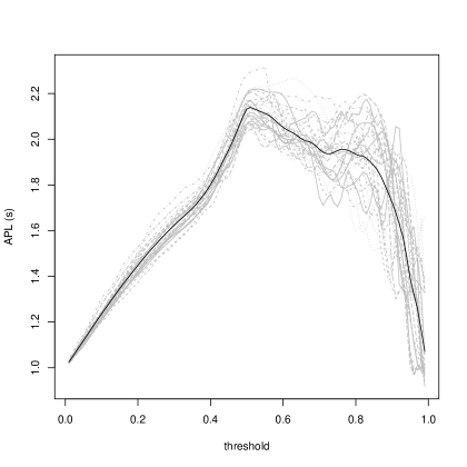
Figure 1: Apnea-data: Smoothed average path length (APL) from 29 patients over different thresholds. Black solid line indicates the mean of APL over thresholds.

This paper is organized as follows. In Section 2, we introduce our varying-coefficient model and propose a local-linear GMM estimator. In Section 3, we present a multi-step estimation procedure. We establish asymptotic results in Section 4. We perform a set of simulations studied to understand the finite sample performance of the proposed estimator and present those in Section 5. In Section 6, we apply the proposed method in a real imaging data-set on obstructive sleep apnea (OSA). In Section 7, we conclude this article with some discussion. All technical details are provided in supplementary material.

2 Varying-coefficient functional model and moment conditions

In this section, we first introduce heteroskedastic conditions for SVC model and thereafter, propose a heuristic method to construct a mean-zero function.

2.1 Model

Let $\{Y_{i}(s),\mathbf{X}_{i}\}$ for $i=1,\cdots,n$ be independent copies of $\{Y(s),\mathbf{X}\}$. Instead of observing the entire functional trajectory, one can observe $Y(s)$ only on the discrete spatial grid $\{s_{1},\cdots,s_{r}\}$ on the functional domain $\mathcal{S}$. Data can be Gaussian or non-Gaussian and homoskedastic or heteroskedastic depending on the real applications. Therefore, the observed data for the $i$-th individual are $\{s_{j},Y_{i}(s_{j}),\mathbf{X}_{i}:j=1,\cdots,r\}$. For simplifying the notation, define $Y_{ij}=Y_{i}(s_{j})$ and $U_{ij}=U_{i}(s_{j})$. Considering the functional principal component analysis (FPCA) model for $U_{i}(s)$, we assume that $U_{i}(s)$ is square-integrable and admits the Karhunen-Loève expansion (Karhunen, 1946; Loève, 1946). Let $\omega_{1}(\mathbf{X})\geq\omega_{2}(\mathbf{X})\geq\cdots\geq 0$ be ordered eigen-values of the linear operator determined by $\Sigma$ with $\sum_{k=1}^{\infty}\omega_{k}(\mathbf{X})$ being finite and $\psi_{k}(s)$’s being the corresponding orthonormal eigen-functions or principal components. Thus, the spectral decomposition (J Mercer, 1909) is given by

$$\Sigma(s,s^{\prime})=\sum_{k=1}^{\infty}\omega_{k}(\mathbf{X})\psi_{k}(s)\psi_{k}(s^{\prime})$$ (2.3)

Therefore, $U_{i}(s)$ admits the Karhunen-Loève expansion as follows.

$$U_{i}(s)=\sum_{k=1}^{\infty}\xi_{k}(\mathbf{X}_{i})\psi_{k}(s)$$ (2.4)

where $\xi_{k}(\mathbf{X}_{i})=\int_{\mathcal{S}}U_{i}(s)\psi_{i}(s)ds$, which is termed as the $k$-th functional principal score for $i$-th individual. The $\xi_{k}(\mathbf{X}_{i})$ are uncorrelated over $k$ with $\mathbb{E}\{\xi_{k}(\mathbf{X}_{i})|\mathbf{X}_{i}\}=0$ and $\text{Var}\{\xi_{k}(\mathbf{X}_{i})|\mathbf{X}_{i}\}=\omega_{k}(\mathbf{X}_{i})$, $k\geq 1$. Furthermore, assume that the eigen-values vary with $\mathbf{X}_{i}$ such that $\omega_{k}(\mathbf{X}_{i})=\theta_{k}\sigma^{2}(\mathbf{X}_{i})$ for some unknown function $\sigma(\mathbf{X})\geq 0$ and $\theta_{1}\geq\theta_{2}\geq\cdots\geq 0$. For identifiability, we need some restrictions on $\theta_{k}$s, such as known or fixed $\theta_{1}$. Therefore, the above assumption on eigen-values for spectral decomposition allow us to incorporate heteroskedasticity into the model. To best of our knowledge, this is the first attempt to model SVC with unknown heteroskedasticity.

2.2 Local-linear mean-zero function

Let us reiterate our main objective: we want to efficiently estimate the varying-coefficient functions based on GMM for the case of continuum moment conditions together with infinite-dimensional parameters. Therefore, we need to construct a mean-zero function which will be described in this sub-section.

Since $\boldsymbol{\beta}(\cdot)$ in model 1.1 is twice continuously differentiable, we can apply the Taylor series expansion to $\boldsymbol{\beta}(s_{j})$ around an interior point $s_{0}$ and get

$$\boldsymbol{\beta}(s_{j})=\boldsymbol{\beta}(s)+\dot{\boldsymbol{\beta}}(s_{0})(s_{j}-s_{0})+\ddot{\boldsymbol{\beta}}(s^{*})(s_{j}-s_{0})^{2}/2$$ (2.5)

where $s^{*}$ lies between $s_{j}$ and $s_{0}$ for all $j=1,\cdots,r$ and $\dot{\boldsymbol{\beta}}$ and $\ddot{\boldsymbol{\beta}}$ denote the gradients of $\boldsymbol{\beta}$ and $\dot{\boldsymbol{\beta}}$ with respect to $s$. Thus, $\boldsymbol{\beta}(s_{j})$ can be approximated as $\beta_{k}(s_{j})\approx\beta(s_{0})+\frac{\partial\beta_{k}(s_{0})}{\partial s}(s_{j}-s_{0})$. So in matrix notation, the first-order Taylor series expansion of the coefficient functions becomes

$$\boldsymbol{\beta}(s_{j})\approx\mathbf{A}(s_{0})\mathbf{z}_{h}(s_{j}-s_{0})$$ (2.6)

where $\mathbf{z}_{h}(s_{j}-s_{0})=\left(1,\frac{s_{j}-s_{0}}{h}\right)^{\text{T}}$ and $\mathbf{A}(s)=[\boldsymbol{\beta}(s_{0}),h\dot{\boldsymbol{\beta}}(s_{0})]$ which is a $p\times 2$ matrix. Hence, applying the approximation procedure in Equation (2.6), we can rewrite model 1.1 as

$$Y_{ij} \approx\mathbf{X}_{i}^{\text{T}}\left\{\mathbf{A}(s)\mathbf{z}_{h}(s_{j}-s_{0})\right\}+U_{ir}$$

$$=\left\{\mathbf{z}_{h}(s_{j}-s_{0})\otimes\mathbf{X}_{i}\right\}^{\text{T}}\operatorname{vec}\{\mathbf{A}(s_{0})\}+U_{ir}$$

$$=\mathbf{W}_{ij}(s_{0})^{\text{T}}\boldsymbol{\gamma}(s_{0})+U_{ir}$$ (2.7)

such that $s_{j}$ are sufficiently close to $s_{0}$, where $\mathbf{W}_{ij}(s_{0})=[\mathbf{z}_{h}(s_{j}-s_{0})\otimes\mathbf{X}_{i}]$ and $\boldsymbol{\gamma}(s_{0})=(\boldsymbol{\beta}(s_{0})^{\text{T}},h\dot{\boldsymbol{\beta}}(s_{0})^{\text{T}})^{\text{T}}$, both of which are vectors of length $2p\times 1$.

Let $K(\cdot)$ be a symmetric probability density function which is used as kernel and $h>0$ be the bandwidth; thus, the re-scaled kernel function is defined as $K_{h}(\cdot)=h^{-1}K(\cdot)$. It is easy to see that for a given location $s_{0}\in\mathcal{S}$, we can construct a least squares estimator of $\boldsymbol{\gamma}(s)$ defined in Equation (2.2) by minimizing the sample version of mean squared error $\mathbb{E}\{[Y_{ij}-\mathbf{W}_{ij}^{\text{T}}(s_{0})\boldsymbol{\gamma}(s_{0})]^{2}|\mathbf{X}_{i}\}$. Let $\mathfrak{M}(\mathbf{X})$ be a $q$-dimensional instrument variable with $q\geq p$; the moment condition can be written as $\mathbb{E}\left\{r^{-1}\sum_{j=1}^{r}K_{h}(s_{j}-s_{0})\boldsymbol{\Delta}_{ij}(s_{0})\right\}=0$ where $\boldsymbol{\Delta}_{ij}(s_{0})=\mathfrak{M}(\mathbf{X}_{i})\left\{Y_{ij}-\mathbf{W}_{ij}(s_{0})^{\text{T}}\boldsymbol{\gamma}(s_{0})\right\}$ is a zero mean stochastic process. Two popular approaches to construct optimal instrument variables are proposed by Newey (1990); Ai and Chen (2003). Due to functional dependence and existence of heteroskedasticity of an unknown form, these approaches can not be undertaken for the model 2.2 that we have considered. Since Taylor series expansion provides a local approximation of the function, we need to incorporate this phenomenon into the instrument variables during construction of the mean-zero function.

Motivated from the idea of local-linear estimator Fan and Gijbels (1996), consider the local-linear instrument variables $\mathbf{Q}_{ir}(s_{0})=(\mathfrak{M}(\mathbf{X}_{i}),\mathfrak{M}(\mathbf{X}_{i})(s_{j}-s_{0})/h)^{\text{T}}$. Therefore, consider the following non-parametrically localizing augmented orthogonal moment conditions for estimating $\boldsymbol{\beta}(s)$.

$$\mathbf{g}_{i}\{\boldsymbol{\gamma}(s_{0})\} =r^{-1}\sum_{j=1}^{r}K_{h}(s_{j}-s_{0})\mathbf{Q}_{ir}(s_{0})\left\{Y_{ij}-\mathbf{W}_{ij}(s_{0})^{\text{T}}\boldsymbol{\gamma}(s_{0})\right\}$$

$$=\begin{pmatrix}r^{-1}\sum_{j=1}^{r}K_{h}(s_{j}-s_{0})\boldsymbol{\Delta}_{ij}(s_{0})\\ r^{-1}\sum_{j=1}^{r}K_{h}(s_{j}-s_{0})\frac{(s_{j}-s_{0})}{h}\boldsymbol{\Delta}_{ij}(s_{0})\end{pmatrix}$$

$$=r^{-1}\sum_{j=1}^{r}K_{h}(s_{j}-s_{0})\mathbf{z}_{h}(s_{j}-s_{0})\otimes\boldsymbol{\Delta}_{ij}(s_{0})$$ (2.8)

and note that $\{\mathbf{g}_{i}(\boldsymbol{\gamma}(s))\}:i=1,\cdots,n\}$ are independent and $\mathbb{E}\{\mathbf{g}_{i}(\boldsymbol{\gamma}(s))\}=\mathbf{0}_{2q\times 1}$ for $s\in\mathcal{S}$.

Most of the varying-coefficient models that exist in the literature assume homoskedasticity in covariates and are limited to weakly dependent non-parametric models (Su et al., 2013; Sun, 2016), that differs significantly in our model assumptions. In contrast, we assume a spatially varying-coefficient model under heteroskedasticity of unknown form.

3 Multi-step estimation procedure

This section develops a multi-step estimation procedure to estimate $\boldsymbol{\beta}(s)$ simultaneously across all $s\in\mathcal{S}$. Essentially, the multi-step procedure can be broken down as, Step-I: an initial estimation; Step-II: estimation of the variance function, mean zero function, and eigen-components and Step-III: GMM estimation. The key ideas of each step are described below.

1. Calculate the least squares estimates of $\boldsymbol{\beta}(s)$ as initial estimates, denoted by $\breve{\boldsymbol{\beta}}(s)$ across all $s\in\mathcal{S}$.

2. Estimate the conditional variance of integrated square residuals non-parametrically, subsequently estimate the covariance of mean-zero function. Estimate the eigen-components using multivariate FPCA.

3. Project the continuous moment conditions onto eigen-functions and then combine them by weighted eigenvalues to incorporate spatial dependence and thus obtain the updated estimate of $\boldsymbol{\beta}(s)$, denoted by $\widehat{\boldsymbol{\beta}}(s)$ across all $s\in\mathcal{S}$.

3.1 Step-I: Initial least squares estimates

We consider a local-linear smoother (Fan and Gijbels, 1996) to obtain an initial estimator of $\boldsymbol{\beta}(\cdot)$ ignoring functional dependencies. In this case, the non-linear least squares function of the model 1.1 can be defined as an objective function given by $\mathcal{J}_{init}\{\boldsymbol{\beta}(\cdot)\}=({nr})^{-1}\sum_{i=1}^{n}\sum_{j=1}^{r}\{Y_{ij}-\mathbf{X}_{i}^{\text{T}}\boldsymbol{\beta}(s_{j})\}^{2}$. By the local-linear smoothing method we estimate $\boldsymbol{\gamma}$ at functional point $s_{0}$, by minimizing

$$\mathcal{J}_{init}\{\boldsymbol{\gamma}(s_{0})\} =({nr})^{-1}\sum_{i=1}^{n}\sum_{j=1}^{r}K_{h}(s_{j}-s_{0})\left\{Y_{ij}-\mathbf{W}_{ij}(s_{0})^{\text{T}}\boldsymbol{\gamma}(s_{0})\right\}^{2}$$ (3.9)

The solution of the above least-squares problem can be expressed as

$$\breve{\boldsymbol{\gamma}}(s_{0}) =\left\{({nr})^{-1}\sum_{i=1}^{n}\sum_{j=1}^{r}K_{h}(s_{j}-s_{0})\mathbf{W}_{ij}(s_{0})\mathbf{W}_{ij}(s_{0})^{\text{T}}\right\}^{-1}$$

$$\qquad\times\left\{({nr})^{-1}\sum_{i=1}^{n}\sum_{j=1}^{r}K_{h}(s_{j}-s_{0})\mathbf{W}_{ij}(s_{0})Y_{ij}\right\}$$ (3.10)

Consequently, the estimator of the coefficient function vector $\boldsymbol{\beta}(s)$ at $s_{0}$ is $\breve{\boldsymbol{\beta}}(s_{0})=[(1,0)\otimes\mathbf{I}_{p}]\breve{\boldsymbol{\gamma}}(s_{0})$. We determine the tuning parameter $h$ by using some data-driven techniques such as cross-validation and generalized cross-validation.

3.2 Step-II: Intermediate steps

Step-II consists of two important steps in determining the class of GMM estimator. First in Step-II.A, we propose a method to obtain optimal instrument variables and therefore estimate the eigen-components which are used in local-linear GMM objective function in Step-III. To estimate eigen-components, we essentially need to use a multivariate version of FPCA which is quite uncommon in the literature. We borrow the method proposed by Wang (2008).

Step-II.A: Choice of instrument variables

Choosing instrument variables is critical, and the required identification condition is $q\geq p$, which ensures that the dimension of $\mathbf{Q}_{ij}(s_{0})$ is at least equal to the dimension of $\boldsymbol{\gamma}(s_{0})$. In our model as discussed in Section 2, the error term has a potential heteroskedasticity of unknown form. We define a set of independent and identically distributed random variables $R_{1},R_{2},\cdots,R_{n}$ for $n$ individuals where $R_{i}=\int U_{i}^{2}(s)ds$ for each $i$, termed as integrated square of residuals, and $\mathbb{E}\{R_{i}|\mathbf{X}_{i}\}=\sigma^{2}(\mathbf{X}_{i})\sum_{k=1}^{\infty}\theta_{k}$. Therefore, consider the following non-parametric regression problem.

$$\log{R_{i}}=\log\sigma^{2}(\mathbf{X}_{i})+\epsilon_{i}$$ (3.11)

where $\epsilon_{i}$ is the mean zero random variable with constant variance. The above model in Equation (3.11) boils down to the problem of estimation of $\log\sigma^{2}(\mathbf{X}_{i})$ by regressing the logarithmic value of the integrated squared residuals variable on the covariates $\mathbf{X}_{i}$. This approach is inspired by Yu and Jones (2004); Wasserman (2006) although used in a different context. Since $U_{i}$s are not observable, we replace $U_{i}$ by an efficient estimate that is obtained from Step-I, viz., $\breve{U}_{i}(s)=Y_{ij}-\mathbf{X}_{i}^{\text{T}}\breve{\boldsymbol{\beta}}(s)$ for all $s\in\mathcal{S}$. For application, this step can easily be implemented using “gam” function available in mgcv package in R to get an estimate of the non-parametric mean function, denoted by $\widehat{\mu}(\mathbf{X})$ and therefore $\widehat{\sigma}^{2}(\mathbf{X})=\exp\{\widehat{\mu}(\mathbf{X})\}$. Given the estimate of $\sigma(\cdot)$, we can, therefore, choose instrument variables as $\mathfrak{M}(\mathbf{X}_{i})=\left(\mathbf{X}_{i},\mathbf{X}_{i}/\widehat{\sigma}^{2}(\mathbf{X}_{i})\right)^{\text{T}}$.

Step-II.B: Estimation of eigen-components

Without loss of generality, assume that the spectrum of functional domain $\mathcal{S}=[0,1]$ and the dimension of mean-zero function $\mathbf{g}(s)=(g_{1}(s),\cdots,g_{d}(s))^{\text{T}}$ is $d$ (in our problem, it equals to $2q$) for simplicity. Note that $\mathbf{g}(s)$ is defined on an interval $[0,1]$ such that $\sum_{l=1}^{d}\int\mathbb{E}\{g_{l}^{2}(s)\}ds$ is finite and the covariance function $\mathbf{C}(s,s^{\prime})=\mathbb{E}\left\{\mathbf{g}\{{\boldsymbol{\gamma}}(s)\}\mathbf{g}\{{\boldsymbol{\gamma}}(s)\}^{\text{T}}\right\}$. Under condition (C6) mentioned in Section 4, using the lining-up method in Wang (2008), define a new stochastic process $e(s)$ on the interval $[0,d]$ with eigen-function $\phi_{e}$ such that, $e(s)=g_{l}(s-(l-1))$ and $\phi_{e}(s)=\phi_{l}(s-(l-1))$ for $l-1\leq s<l$, $l=1,\cdots d$, where we define the eigen-function for each $g_{l}$ as $\phi_{l}$ for $l=1,\cdots,d$. Therefore, the covariance function between $g_{l}(s)$ and $g_{l^{\prime}}(s^{\prime})$ can be expressed as $C_{l,l^{\prime}}(s,s^{\prime})=\text{cov}\{g_{l}(s-(l-1)),g_{l^{\prime}}(s^{\prime}-(l^{\prime}-1))\}$ for $l-1\leq s<l$ and $l^{\prime}-1\leq s^{\prime}<l^{\prime}$; $l,l^{\prime}=1,\cdots,d$. Note that, for $d$-dimensional processes the Fredholm integral equation is equivalent to $d$-simultaneous integral equations where each of them corresponds to a specific functional interval of $e(s)$. For $l-1\leq s<l$; $l=1,\cdots,d$, the Fredholm integral equation yields $\int_{0}^{d}\text{cov}\{e(s),e(s^{\prime})\}\phi_{e}(s)ds=\lambda\phi_{e}(s)$. Now observe for $(l-1)\leq s<l;l=1,\cdots,d$, the above relation is equivalent to the following.

$$\sum_{l^{\prime}=1}^{d}\int_{l^{\prime}-1}^{l^{\prime}}\text{cov}\{g_{l}(s-(l-1)),g_{l^{\prime}}(s^{\prime}-(l^{\prime}-1))\phi_{l^{\prime}}(s^{\prime})ds^{\prime}=\lambda\phi_{l}(s-(l-1))$$

$$\sum_{l^{\prime}=1}^{d}\int_{0}^{1}\text{cov}\{g_{l}(s-(l-1)),g_{l^{\prime}}(s^{\prime})\}\phi_{l^{\prime}}(s^{\prime})ds^{\prime}=\lambda\phi_{l}(s-(l-1))$$

$$\sum_{l^{\prime}=1}^{d}\int_{0}^{1}\text{cov}\{g_{l}(s),g_{l^{\prime}}(s^{\prime})\}\phi_{l^{\prime}}(s^{\prime})ds^{\prime}=\lambda\phi_{l}(s)$$ (3.12)

In multivariate setting, the orthogonality condition is

$$\int_{0}^{d}\phi_{e,l}(s)\phi_{e,l^{\prime}}(s)ds=\textbf{1}(l=l^{\prime}) =\sum_{k=1}^{d}\int_{k-1}^{k}\phi_{k,l}(s-(k-1))\phi_{k,l^{\prime}}(s-(k-1))ds$$

$$=\sum_{k=1}^{d}\int_{0}^{1}\phi_{k,l}(s)\phi_{k,l^{\prime}}(s)ds$$ (3.13)

Using the generalized Mercer’s theorem (J Mercer, 1909), the results for the covariance function can be briefly shown using the lining-up method. Assume that the covariance function is continuous after the lining up processes, so for $(l_{1}-1)\leq s<l_{1}$ and $(l_{2}-1)\leq s<l_{2}$; $l_{1},l_{2}=1,\cdots,d$, the covariance function between $g_{l_{1}}(s)$ and $g_{l_{2}}(s^{\prime})$ can be expressed as

$$C_{l,l^{\prime}}(s,s^{\prime}) =\text{cov}\{g_{l}(s),g_{l^{\prime}}(s)\}=\sum_{k=1}^{\infty}\lambda_{k}\phi_{k,l}(s-(l-1))\phi_{k,l^{\prime}}(s-(l^{\prime}-1))$$

$$=\sum_{k=1}^{\infty}\lambda_{k}\phi_{k,l}(s)\phi_{k,l^{\prime}}(s^{\prime})$$ (3.14)

Therefore, using the above argument, we can define the multivariate spectral decomposition $\mathbf{C}(s,s^{\prime})=\sum_{k=1}^{\infty}\lambda_{k}\boldsymbol{\phi}_{k}(s)\boldsymbol{\phi}_{k}(s^{\prime})^{\text{T}}$ with the orthogonality condition 3.2. Since the lining-up data are univariate, we can adopt the existing techniques of estimating functional eigen-values and eigen-function in the literature (Yao et al., 2003; Yao et al., 2005; Müller and Yao, 2010; Li and Hsing, 2010) to estimate $\lambda$ and $\phi_{e}(s)$, and hence can estimate $\boldsymbol{\phi}(s)$ by stacking all components for aliened eigen-functions $\phi_{e}(s)$.

3.3 Step-III: Final estimates

Finally, we demonstrate our proposed estimator based on local-linear GMM where the proposed mean-zero function can be projected onto eigen-function and then combined by the weighted eigen-values. Then, for any positive $\alpha$, the objective function is given by

$$\mathcal{J}\{\boldsymbol{\gamma}(s_{0})\} =\sum_{k=1}^{\infty}\frac{\widehat{\lambda}_{k}}{\widehat{\lambda}_{k}^{2}+\alpha}\left\{\overline{\mathbf{g}}(\boldsymbol{\gamma}(s_{0}))^{\text{T}}\widehat{\boldsymbol{\phi}}_{k}(s_{0})\right\}^{2}$$

$$=\sum_{k=1}^{\infty}\frac{\widehat{\lambda}_{k}}{\widehat{\lambda}_{k}^{2}+\alpha}\left\{({nr})^{-1}\sum_{i=1}^{n}\sum_{j=1}^{r}K_{h}(s_{j}-s_{0})\widehat{\boldsymbol{\phi}}_{k}(s_{0})^{\text{T}}\mathbf{Q}_{ij}(s_{0})\left[Y_{ij}-\mathbf{W}_{ij}(s_{0})^{\text{T}}\boldsymbol{\gamma}(s_{0})\right]\right\}^{2}$$ (3.15)

By minimizing the above objective function, we obtain

$$\sum_{k=1}^{\infty}\frac{\widehat{\lambda}_{k}}{\widehat{\lambda}_{k}^{2}+\alpha}\left\{({nr})^{-1}\sum_{i=1}^{n}\sum_{j=1}^{r}K_{h}(s_{j}-s_{0})\widehat{\boldsymbol{\phi}}_{k}(s_{0})^{\text{T}}\mathbf{Q}_{ij}(s_{0})\mathbf{W}_{ij}(s_{0})\right\}$$

$$\qquad\times\left\{({nr})^{-1}\sum_{i=1}^{n}\sum_{j=1}^{r}K_{h}(s_{j}-s_{0})\widehat{\boldsymbol{\phi}}_{k}(s_{0})^{\text{T}}\mathbf{Q}_{ij}(s_{0})\left[Y_{ij}-\mathbf{W}_{ij}(s_{0})^{\text{T}}\boldsymbol{\gamma}(s_{0})\right]\right\}$$

$$:=\sum_{k=1}^{\infty}\frac{\widehat{\lambda}_{k}}{\widehat{\lambda}_{k}^{2}+\alpha}\mathcal{X}_{k}(s_{0})\left\{\mathcal{Y}_{k}(s_{0})-\mathcal{X}_{k}(s_{0})^{\text{T}}\boldsymbol{\gamma}(s_{0})\right\}$$ (3.16)

where $\mathcal{X}_{k}(s_{0})=({nr})^{-1}\sum_{i=1}^{n}\sum_{j=1}^{r}K_{h}(s_{j}-s_{0})\widehat{\boldsymbol{\phi}}_{k}(s_{0})^{\text{T}}\mathbf{Q}_{ij}(s_{0})\mathbf{W}_{ij}(s_{0})$ and $\mathcal{Y}_{k}(s_{0})=({nr})^{-1}\sum_{i=1}^{n}\sum_{j=1}^{r}K_{h}(s_{j}-s_{0})\widehat{\boldsymbol{\phi}}_{k}(s_{0})^{\text{T}}\mathbf{Q}_{ij}(s_{0})Y_{ij}$. Therefore, the final estimate of the coherent function is $\widehat{\boldsymbol{\beta}}(s_{0})=[(1,0)\otimes\mathbf{I}_{p}]\widehat{\boldsymbol{\gamma}}(s_{0})$ where

$$\widehat{\boldsymbol{\gamma}}(s_{0})=\left\{\sum_{k=1}^{\infty}\frac{\widehat{\lambda}_{k}}{\widehat{\lambda}_{k}^{2}+\alpha}\mathcal{X}_{k}(s_{0})\mathcal{X}_{k}(s_{0})^{\text{T}}\right\}^{-1}\left\{\sum_{k=1}^{\infty}\frac{\widehat{\lambda}_{k}}{\widehat{\lambda}_{k}^{2}+\alpha}\mathcal{X}_{k}(s_{0})\mathcal{Y}_{k}(s_{0})\right\}$$ (3.17)

The algorithm 1 summarizes the proposed method. For demonstration purposes, we choose the tuning parameters using cross-validation as discussed in the algorithm. In the proposed algorithm, $\alpha$ controls the number of eigen-values, and can be chosen so that condition (C8) defined in Section 4 is valid. Moreover, a continuity condition for lining-up is required for theoretical justification, by empirical studies, in the present of discontinuity in $\phi_{e}$, the end results are still adequate to use in practice.

Algorithm 1 Estimation of $\boldsymbol{\beta}(s):s\in\mathcal{S}$

1:$\{Y_{i}(s_{j}),X_{i},s_{j}\}$, for $j=1,\cdots,r;i=1,\cdots,n$

2:Calculate optimal $h$: $\widehat{h}_{init}\leftarrow\arg\min_{h\in\mathcal{H}}({nr})^{-1}\sum_{i=1}^{n}\sum_{r=1}^{r}\left\{Y_{ij}-\mathbf{X}_{i}^{\text{T}}\breve{\boldsymbol{\beta}}^{-i}(s_{r};h)\right\}^{2}$

3:Calculate $\breve{\boldsymbol{\gamma}}(s;\widehat{h}_{init})$

4:Compute $\mathbf{g}_{i}\{\boldsymbol{\gamma}(s)\}=r^{-1}\sum_{j=1}^{r}K_{\widehat{h}_{init}}(s_{j}-s)\mathbf{Q}_{ij}(s;\widehat{h}_{init})\{Y_{ij}-\mathbf{W}_{ij}(s;\widehat{h}_{init})^{\text{T}}\breve{\boldsymbol{\gamma}}(s;\widehat{h}_{init})\}$

5:Determine the instrument variables $\mathfrak{M}(\mathbf{X})$

6:Compute eigen-components $\widehat{\lambda}_{k},\widehat{\boldsymbol{\phi}}_{k}(s)$ and get the value of $\alpha$ using the condition (C8).

7:Calculate optimal $h$: $\widehat{h}_{opt}\leftarrow\arg\min_{h\in\mathcal{H}}({nr})^{-1}\sum_{i=1}^{n}\sum_{r=1}^{r}\left\{Y_{ij}-\mathbf{X}_{i}^{\text{T}}\widehat{\boldsymbol{\beta}}^{-i}(s_{r};h)\right\}^{2}$

8:Calculate $\widehat{\boldsymbol{\beta}}(s;h_{opt})$

4 Asymptotic results

In this section, we provide some assumptions and then study the asymptotic properties of the local-linear GMM estimator. Here, we allow the sample size $n$ and number of functional domains $r$ to grow to infinity. Detailed technical proofs are provided in the online Supplementary Material.

Let $\boldsymbol{\beta}_{0}(s_{0})$ be the true value of $\boldsymbol{\beta}(s_{0})$ at location $s_{0}$. For simplicity, define, $\delta_{n1}(h)=\left\{(1+(hr)^{-1})\log n/n\right\}^{1/2}$ and $\delta_{n2}(h)=\left\{(1+(hr)^{-1}+(hr)^{-2})\log n/n\right\}^{1/2}$. $\nu_{a,b}=\int t^{a}K^{b}(t)dt$. Consider the following conditions that will be useful in asymptotic results.

1. Kernel function $K(\cdot)$ is a symmetric density function defined on the bounded support $[-1,1]$ and is Lipschitz continuous.

2. Density function $f_{T}$ of $T$ is bounded above and away from infinity, and also below and away from zero. Moreover, $f$ is differentiable and the derivative is continuous.

3. $\mathbb{E}\{\|X\|^{a}\}<\infty$ and $\mathbb{E}\{\sup_{s\in\mathcal{S}}|U(s)|^{a}\}<\infty$ for some positive $a>1$. Define, $\mathbb{E}\{\mathfrak{M}(\mathbf{X})\mathbf{X}\}=\boldsymbol{\Omega}$ with rank $p$.

4. The true coefficient function $\boldsymbol{\beta}_{0}(s)$ is three-times continuously differentiable and $\Sigma(s,s^{\prime})$ are twice continuously differentiable.

5. $\{U(s):s\in[0,1]\}$ and $\{\mathfrak{M}(\mathbf{X})U(s):s\in[0,1]\}$ are Donsker class, where $\mathbf{X}\subset\mathfrak{M}(\mathbf{X})$.

6. 1. $\lim_{s\searrow 1}\mathbb{E}\{|g_{l}(s-1)-g_{l}(0)|^{2}\}=0$ for $l=1,\cdots,d$

   2. $\lim_{s\nearrow 1}\mathbb{E}\{|g_{l-1}(s)-g_{l}(0)|^{2}\}=0$ for $l=2,\cdots,d$

7. All second order partial derivatives of $\mathbf{C}(s,s^{\prime})$ exist and are bounded on the support of the functional domain.

8. For some $\kappa_{0}\geq 1$ and $\alpha^{-1}=o\left(\sum_{k=1}^{\kappa_{0}}\lambda_{k}^{-1}/\sum_{k=\kappa_{0}+1}^{\infty}\lambda_{k}\right)$

9. The numbers of individuals and functional grid-points are growing to infinity such that $h\rightarrow 0$ and $rh\rightarrow\infty$. For some positive number $a\in(2,4)$, $|\log h|^{1-2/a}/h\leq r^{1-2/a}$. For $a>2$, $(h^{4}+h^{3}/r+h^{2}/r^{2})^{-1}(\log n/n)^{1-2/a}\rightarrow 0$ as $n\rightarrow\infty$.

Remark 1.

Conditions (C1) and (C2) are commonly used in the literature of non-parametric regression. The bound condition for the density function in (C2) of functional points is standard for random design. Similar results can be obtained for fixed design where the grid-points are pre-fixed according to the design density $\int_{0}^{s_{j}}f(s)dt=j/r$ for $j=1,\cdots,r$, for $r\geq 1$. The condition (C3) is similar to that in Li and Hsing (2010) which requires the bound on the higher order moment of $\mathbf{X}$. Moreover the condition on rank of $\boldsymbol{\Omega}$ is required for identification of the functional coefficient and its first order derivatives (Su et al., 2013). Condition (C4) is also common in functional data analysis literature (Wang et al., 2016). This condition allows us to perform Taylor series expansion. Condition in (C5) avoids the smoothness condition of the sample path (Zhu et al., 2012, 2014) which are commonly assumed in Hall and Hosseini-Nasab (2006); Zhang and Chen (2007); Cardot et al. (2013). Conditions (C6) are required to check the continuity in the mean-zero function, which is equivalent to check the mean square continuity of the process after lining up (Hadinejad-Mahram et al., 2002). Here, the first condition shows the limits from right and remain always right; therefore, it involves only one process. A similar, but opposite, phenomenon occurs in the second condition. Moreover, if the vector process $\mathbf{g}(s)$ is mean-square continuous then both approaches are equivalent, as a result, the covariance function is continuous after lining-up the process. To obtain the asymptotic expression of $\widehat{\boldsymbol{\beta}}(s)$, observed for fixed sample size, there exists $\kappa_{0}$ such that $k\leq\kappa_{0}$, $\lambda_{k}^{2}$ is much larger than $\alpha$, thus, the ratio $\lambda_{k}/(\lambda_{k}^{2}+\alpha)\approx\lambda_{k}^{-1}$. On the other hand, if $k>\kappa_{0}$, $\lambda_{k}^{2}<<\alpha$, as a result, the fraction $\lambda_{k}/(\lambda_{k}^{2}+\alpha)$ can be approximately written as $\lambda_{k}/\alpha$. Therefore, by the assumption that we make in (C8), we can write, for $s\in\mathcal{S}$,

$$\sum_{k=1}^{\kappa_{0}}\lambda_{k}^{-1}\boldsymbol{\phi}_{k}(s)\boldsymbol{\phi}_{k}(s^{\prime})^{\text{T}}+\alpha^{-1}\sum_{k=\kappa_{0}+1}^{\infty}\lambda_{k}\boldsymbol{\phi}_{k}(s)\boldsymbol{\phi}_{k}(s^{\prime})^{\text{T}}=\sum_{k=1}^{\kappa_{0}}\lambda_{k}^{-1}\boldsymbol{\phi}_{k}(s)\boldsymbol{\phi}_{k}(s^{\prime})^{\text{T}}\left\{1+o(1)\right\}$$ (4.18)

Condition (C9) provide the range of bandwidth. Under the fixed sampling design, this condition can be weakened, see Zhu et al. (2012).

The the following result provide the asymptotic properties of the initial estimates mention in Step-I.

Theorem 1.

Under conditions (C1), (C2), (C3), (C4), (C5), and (C9)

$\Big{\{}\sqrt{n}\left(\breve{\boldsymbol{\beta}}(s_{0})-\boldsymbol{\beta}_{0}(s_{0})-0.5h^{2}\nu_{21}\ddot{\boldsymbol{\beta}}_{0}(s_{0})\right)\Big{.}$ $\Big{.}\times(1+o_{a.s.}(1)):s_{0}\in\mathcal{S}\Big{\}}$ weakly converges to a mean zero Gaussian process with a covariance matrix $\Sigma(s_{0},s_{0})\boldsymbol{\Omega}_{\mathbf{x}}^{-1}$ where $\boldsymbol{\Omega}_{\mathbf{x}}=\mathbb{E}\{\mathbf{X}\mathbf{X}^{\text{T}}\}$.

Next, we study the convergence rates of the estimated eigen-components based on the proposed lining-up method. The following lemma is output of the asymptotic expansion of eigen-components of an estimated covariance function.

Lemma 1.

Under assumptions (C1), (C2), (C3), (C6), (C7), (C8), and (C9) the following convergence holds almost surely for any finite-dimensional mean-zero function $\mathbf{g}(s)$.

1. $\left|\widehat{\lambda}_{k}-\lambda_{k}\right|=O(h^{2}+\delta_{n1}(h)+\delta_{n2}(h))$

2. $\sup_{s_{0}\in\mathcal{S}}\left|\widehat{\boldsymbol{\phi}}_{k}(s_{0})-\boldsymbol{\phi}_{k}(s_{0})\right|=O(h^{2}+\delta_{n1}(h)+\delta_{n2}^{2}(h))$

for all $k=1,\cdots,\kappa_{0}$.

We skip the proof of the above lemma as it is well-developed in the literature of functional data analysis including Hall (2004); Hall and Hosseini-Nasab (2006); Li and Hsing (2010). Next, we show the asymptotic results of the proposed estimation.

Theorem 2.

Suppose the conditions (C1), (C2), (C3), (C4), (C5), (C6), (C7), (C8), and (C9) hold, then for the proposed local-linear GMM estimator $\widehat{\boldsymbol{\beta}}(s)$, have the following results hold.

$\left\{\sqrt{n}\left(\widehat{\boldsymbol{\beta}}(s)-\boldsymbol{\beta}_{0}(s)-0.5h^{2}\nu_{21}\ddot{\boldsymbol{\beta}}(s))\right)(1+o_{a.s.}(1)):s\in\mathcal{S}\right\}$ weakly converges to a mean zero Gaussian process with a covariance matrix

$$\mathcal{A}(s_{0},s_{0})=\left(\boldsymbol{\Omega}\mathbf{C}_{\kappa_{0},11}^{-1}(s_{0},s_{0})\boldsymbol{\Omega}^{\text{T}}\right)^{-1}\boldsymbol{\Omega}\mathbf{C}_{\kappa_{0},11}^{-1}(s_{0},s_{0})\boldsymbol{\Sigma}(s_{0},s_{0})\mathbf{C}_{\kappa_{0},11}^{-1}(s_{0},s_{0})\boldsymbol{\Omega}\left(\boldsymbol{\Omega}\mathbf{C}_{\kappa_{0},11}(s_{0},s_{0})^{-1}\boldsymbol{\Omega}^{\text{T}}\right)^{-1}$$

.

5 Simulation studies

We conduct numerical studies to compare finite sample performance under different correlation structures and heterogeneity conditions. Data are generated from the model $Y_{i}(s)=X_{i}\boldsymbol{\beta}(s)+U_{i}(s)$. where we generate trajectories observed at $r$ spatial locations for $i$-th curve, $i=1,\cdots,n$. Assume that the functional fixed effect be $\beta(s)=\cos(2\pi s)$ and corresponding fixed effect covariate is generated from normal distribution with unit mean and variance. The error process is generated as $U_{i}(s)=\xi_{1}(X_{i})\psi_{1}(s)+\xi_{2}(X_{i})\psi_{2}(s)$ where $\xi_{1}(X_{i})$ and $\xi_{2}(X_{i})$ are independent central normal random variables with variance $3\sigma^{2}(X_{i})\theta_{0}^{2}$ and $1.5\sigma^{2}(X_{i})\theta_{0}^{2}$ where $\theta_{0}$ is determined by the relative importance of random error signal-to-noise ratio, denoted as $\text{SNR}_{\theta}$ which is interpreted as the ratio of standard deviation of the additive prediction without noise divided by the standard error of the random noise function. For example, $\text{SNR}_{\theta}=2$ means that the contribution of each functional random noise to the variability in $Y(s)$ is about double than the fixed effect (Scheipl et al., 2015). Here, we use scaled orthonormal functions $\psi_{1}(s)\propto(1.5-\sin(2\pi s)-\cos(2\pi s))$ and $\psi_{2}(s)\propto\sin(4\pi s)$; due to orthonormality, the proportionality constant can easily be determined. Contributions to the conditional variances in $\xi_{k}(X)$ are specified as (S.0) $\sigma^{2}(x)=1$ (homoskedastic), (S.1) $\sigma^{2}(x)=(1+x^{2}/2)^{2}$, (S.2) $\sigma^{2}(x)=\exp(1+x^{2}/2)$, (S.3) $\sigma^{2}(x)=\exp(1+|{x}|+x^{2})$ and (S.4) $\sigma^{2}(x)=(1+|x|/2)^{2}$. We sample the trajectories at $r$ equidistant spatial points $\{s_{1},\cdots,s_{r}\}$ on $[0,1]$. Let $s_{i}=(j-0.5)/r$ for $j=1,\cdots,r$ for $i$-th curve. The number of spatial points is assumed to be 200 for each case. We set number of trajectories $n\in\{50,100,200,500\}$ and the controlling parameter $\theta_{0}$ is determined using signal-to-noise ratio, $\text{SNR}_{\theta}$ which is assumed to be either 0.5 or 1. Here, we perform 500 simulation replicates. To make it consistent with theoretical results and numerical examples, we use “FPCA” function in R which is available in fdapace package (Gajardo et al., 2021) to estimate the eigen-functions. Bandwidths are selected using five-fold generalized cross-validation in all situations and for estimation, the Epanechnikov kernel $K(x)=0.75(1-x^{2})_{+}$ is used; where $(a)_{+}=\max(a,0)$. Accuracy of the parameter estimation is assessed using integrated mean square error which for the $b$-th replication is defined as $\text{IMSE}_{b}=\left[\sum_{j=1}^{r}\left(\widehat{\boldsymbol{\beta}}_{b}(s_{j})-\boldsymbol{\beta}(s_{j})\right)^{2}\Delta(s_{r})\right]$ and integrated mean absolute error $\text{IMAE}_{b}=\left[\sum_{j=1}^{r}|\widehat{\boldsymbol{\beta}}_{b}(s_{j})-\boldsymbol{\beta}(s_{j})|\Delta(s_{r})\right]$ with $\Delta(s_{j})=s_{j}-s_{j-1}$ and $s_{0}=0$ and $s_{1}<\cdots<s_{r}$ are the observed points over the support set of observational points. We have noticed that the results can be improved by multiplying $h^{*}$ by a constant in a certain range where $h^{*}$ is the optimal bandwidth obtained from cross validation. We use $\widehat{\boldsymbol{\beta}}$ corresponding to bandwidth $0.75h^{*}$ for our numerical studies. We present Tables 1 and 2 where IMSEs and IMAEs are averaged over 500 replications for each situation. We denote LLE and LLGMM by local-linear smoothing estimator described in Step-I and local-linear GMM with weight matrix as proposed in Step-III in Section 3 respectively. As expected, for all situations, the IMSE and IMAE are significantly reduced if we increase sample size and/or $\text{SNR}_{\theta}$. For homoskedastic case, the error rates of LLE are similar for LLGMM but under the presence of heteroskedasticity of unknown form, our proposed method outperforms.

Table 1: Performance of the estimation procedure with $\text{SNR}_{\theta}=0.5$

		n = 50		n = 100		n = 200		n = 500
Case	Method	IMSE	IMAE	IMSE	IMAE	IMSE	IMAE	IMSE	IMAE
S.0	LLE	0.0372	0.1429	0.0189	0.1016	0.0099	0.0737	0.0041	0.0472
	LLGMM	0.0388	0.1460	0.0198	0.1038	0.0100	0.0740	0.0042	0.0474
S.1	LLE	0.0939	0.2271	0.0516	0.1679	0.0261	0.1189	0.0106	0.0766
	LLGMM	0.0585	0.1820	0.0292	0.1262	0.0135	0.0867	0.0050	0.0517
S.2	LLE	0.1381	0.2810	0.0812	0.2169	0.0468	0.1632	0.0209	0.1094
	LLGMM	0.0557	0.1462	0.0134	0.0817	0.0045	0.0471	0.0015	0.0262
S.3	LLE	0.1762	0.3330	0.1018	0.2538	0.0581	0.1913	0.0265	0.1291
	LLGMM	0.1067	0.0600	0.0021	0.0201	0.0004	0.0093	0.0003	0.0064
S.4	LLE	0.0588	0.1798	0.0309	0.1298	0.0158	0.0928	0.0065	0.0596
	LLGMM	0.0576	0.1792	0.0303	0.1287	0.0153	0.0914	0.0063	0.0585

Table 2: Performance of the estimation procedure with $\text{SNR}_{\theta}=1$

		n = 50		n = 100		n = 200		n = 500
Case	Method	IMSE	IMAE	IMSE	IMAE	IMSE	IMAE	IMSE	IMAE
S.0	LLE	0.0097	0.0729	0.0048	0.0515	0.0025	0.0372	0.0010	0.0237
	LLGMM	0.0101	0.0741	0.0052	0.0532	0.0025	0.0374	0.0010	0.0238
S.1	LLE	0.0248	0.1169	0.0135	0.0860	0.0068	0.0608	0.0027	0.0387
	LLGMM	0.0126	0.0836	0.0062	0.0573	0.0029	0.0403	0.0012	0.0253
S.2	LLE	0.0363	0.1440	0.0215	0.1117	0.0124	0.0842	0.0055	0.0560
	LLGMM	0.0069	0.0589	0.0029	0.0376	0.0012	0.0239	0.0004	0.0142
S.3	LLE	0.0466	0.1705	0.0274	0.1314	0.0157	0.0994	0.0071	0.0669
	LLGMM	0.0006	0.0133	0.0003	0.0078	0.0002	0.0069	0.0001	0.0052
S.4	LLE	0.0155	0.0924	0.0080	0.0662	0.0041	0.0472	0.0016	0.0300
	LLGMM	0.0142	0.0883	0.0074	0.0634	0.0037	0.0449	0.0015	0.0285

6 Real data analysis

For illustrating the application of our proposed method and the estimation procedure therein, we use Apnea-data to understand white matter structural alterations using diffusion tensor imaging (DTI) in obstructive sleep apnea (OSA) patients (Xiong et al., 2017). The data consist of 29 male patients (age range: 30-55 years) who underwent the study for the diagnosis of continuous positive airway pressure (CPAP) therapy. DTI was performed at 3T, followed by the analysis using tract-based spatial statistics to investigate the difference in fractional anisotropy (FA) and other diffusion properties between the groups based on lapses. The image acquisition is as follows. Images are recorded on a 3T MRI scanner using a commercial 32-channel head coil. An axial T1-weighted image of the brain (3D-BRAVO) is collected with repetition time (TR) = 12ms, echo time (TE) = 5,2ms, flip angle = $13^{\circ}$, inversion time = 450 ms, matrix = $384\times 256$, voxel size = $1.2\times 0.57\times 0.69$mm and scan time = 2 min 54 sec. DTI are obtained in the axial plane using a spin-echo echo planner imaging sequence with TR = 4500ms, TE = 89.4ms, field of view = $20\times 20$cm², matrix size = $160\times 132$, slice thickness = 3mm, slice spacing = 1mm, b-values = 0, 1000 s/mm².

FA varies systematically along the trajectory of each white matter fascicle. Several pre- and post-processing steps were performed by the FSL software. The brain was extracted using brain segmentation tools. After generating FA maps using FMRIB diffusion toolbox, images from all individuals were aligned to an FA standard template through non-linear co-registration. The Johns Hopkins University (JHU) white matter tractography atlas was used as a standard template for white matter parcellation with 50 regions of interest (ROIs). All imaging parameters were calculated by averaging the voxel values in each ROI.

For each subject, we calculate the similarity matrix $\mathbf{C}$ with dimension $50\times 50$. The $(k,l)$-th element of the matrix $\mathbf{C}$ is defined as $c_{kl}=|y_{k}-y_{l}|$ where $y_{k}$ is the measure of FA associated with $k$-th ROI. For simplicity, we scale the similarity matrix such that the range of the elements of the matrix is $[0,1]$. To create the network, we threshold each similarity matrix to build an adjacency matrix $\mathbf{G}$ with elements $\{1,0\}$ depending on whether the similarity values exceed the threshold or not. Since this threshold controls the topology of the data, we contract the adjacent matrix over a set of threshold parameters from 0.01 to 0.99, and this set is denoted as $\mathcal{S}$ with cardinally $99$. A popular measure of the connectivity is average path length (APL) which is defined as the average number of steps along the shortest path for all possible pairs of the network nodes. Therefore it measures the efficacy of the information on a network (Albert and Barabási, 2002). For a series of threshold parameters $(s)$, we observe APL for FA as shown in Figure 1. Scientists are often interested to know the association of APL of the network generated from FA with a set of covariates of interests such as age and lapses score.

We fit the model 1.1 to APL that are collected over continuous spatial domains (viz, thresholds) from all individuals in which $\mathbf{X}_{i}$ included the clinical variables such as lapses, age. We discard the subjects from the analysis with missing clinical variables and therefore the sample size $n=27$. Here we used three-fold cross validation to obtain the tuning parameters and the FVE is set be at 0.99. In Figure 2, we present the estimated coefficient functions corresponding to age and number of lapses associated with APL where it can be observed that the coefficient of network property is negative with age but positive with lapses counts. Moreover the effect for the APL is found to be increasing when the significance level is small to moderate and decreasing at moderate to large significance levels; whereas, the effect of APL is more-or-less similar upto the larger values of threshold, and after that it significantly decreases. Here small values of significant thresholds represent sparse connected graph where the true connection might be eliminated due to lenient thresholding, on the other hand for large significant values, the generated graphs are densely connected.

Figure 2: Apnea-data analysis: Plots of estimated coefficient functions of age (top panel) and number of lapses (bottom panel) for average path length associated with Fractional Anisotropy (FA) in DTI analysis

7 Discussion

In this article, we propose an efficient estimation procedure for varying-coefficient model which is commonly used in neuroimaging and econometrics. We understand that this procedure is an efficient approach to incorporate heteroskedasticity in the analysis of functional data. To best of our knowledge, this the first initiative to incorporate such condition into the model. Such model is therefore equipped with more complex relationship between the functional response and real-valued covariates. Additionally, our method is easy to implement in a wide range of applications due to the multi-stage structure of the algorithm. The applicability of the proposed method is illustrated by the simulation studies and real data analysis.

Supplementary material

Contains a brief description of the theoretical proofs of the theorems proposed in Section 4.

Department of Statistics and Probability, Michigan State University, Wells Hall, 619 Red Cedar Rd, East Lansing, MI 48824, USA E-mail: (guhaniyo@msu.edu) Department of Mathematics, Statistics and Computer Science, University of Illinois at Chicago, 851 S. Morgan Street, Chicago, Illinois 60607, USA E-mail: (pszhong@uic.edu) Center for MR Research and Departments of Radiology, Neurosurgery, and Bioengineering, University of Illinois at Chicago, 1801 West Taylor St., Chicago, Illinois 60612, USA E-mail: (xjzhou@uic.edu)

References

- Ai and Chen (2003) Ai, C. and X. Chen (2003). Efficient estimation of models with conditional moment restrictions containing unknown functions. Econometrica 71(6), 1795–1843.
- Albert and Barabási (2002) Albert, R. and A.-L. Barabási (2002). Statistical mechanics of complex networks. Reviews of modern physics 74(1), 47.
- Bravo (2021) Bravo, F. (2021). Second order expansions of estimators in nonparametric moment conditions models with weakly dependent data. Econometric Reviews, 1–24.
- Cai et al. (2006) Cai, Z., M. Das, H. Xiong, and X. Wu (2006). Functional coefficient instrumental variables models. Journal of Econometrics 133(1), 207–241.
- Cai and Li (2008) Cai, Z. and Q. Li (2008). Nonparametric estimation of varying coefficient dynamic panel data models. Econometric Theory 24(5), 1321–1342.
- Cardot et al. (2013) Cardot, H., D. Degras, and E. Josserand (2013). Confidence bands for horvitz–thompson estimators using sampled noisy functional data. Bernoulli 19(5A), 2067–2097.
- Chiou et al. (2004) Chiou, J.-M., H.-G. Müller, and J.-L. Wang (2004). Functional response models. Statistica Sinica, 675–693.
- Cragg (1983) Cragg, J. G. (1983). More efficient estimation in the presence of heteroscedasticity of unknown form. Econometrica: Journal of the Econometric Society, 751–763.
- Delaigle and Hall (2010) Delaigle, A. and P. Hall (2010). Defining probability density for a distribution of random functions. The Annals of Statistics, 1171–1193.
- Fan and Gijbels (1996) Fan, J. and I. Gijbels (1996). Local polynomial modelling and its applications. Chapman & Hall/CRC.
- Fan et al. (2003) Fan, J., Q. Yao, and Z. Cai (2003). Adaptive varying-coefficient linear models. Journal of the Royal Statistical Society: series B (statistical methodology) 65(1), 57–80.
- Fan and Zhang (2008) Fan, J. and W. Zhang (2008). Statistical methods with varying coefficient models. Statistics and its Interface 1(1), 179.
- Fan et al. (1999) Fan, J., W. Zhang, et al. (1999). Statistical estimation in varying coefficient models. The annals of Statistics 27(5), 1491–1518.
- Gajardo et al. (2021) Gajardo, A., C. Carroll, Y. Chen, X. Dai, J. Fan, P. Z. Hadjipantelis, K. Han, H. Ji, H.-G. Mueller, and J.-L. Wang (2021). fdapace: Functional Data Analysis and Empirical Dynamics. R package version 0.5.7.
- Hadinejad-Mahram et al. (2002) Hadinejad-Mahram, H., D. Dahlhaus, and D. Blomker (2002). Karhunen-loéve expansion of vector random processes. Technical report, Technical Report No. IKTNT 1019, Communications Technological Laboratory.
- Hall (2004) Hall, A. R. (2004). Generalized method of moments. OUP Oxford.
- Hall and Hosseini-Nasab (2006) Hall, P. and M. Hosseini-Nasab (2006). On properties of functional principal components analysis. Journal of the Royal Statistical Society: Series B (Statistical Methodology) 68(1), 109–126.
- Hansen (1982) Hansen, L. P. (1982). Large sample properties of generalized method of moments estimators. Econometrica: Journal of the Econometric Society, 1029–1054.
- Hastie and Tibshirani (1993) Hastie, T. and R. Tibshirani (1993). Varying-coefficient models. Journal of the Royal Statistical Society: Series B (Methodological) 55(4), 757–779.
- J Mercer (1909) J Mercer, B. (1909). Xvi. functions of positive and negative type, and their connection the theory of integral equations. Phil. Trans. R. Soc. Lond. A 209(441-458), 415–446.
- Karhunen (1946) Karhunen, K. (1946). Zur spektraltheorie stochastischer prozesse. Ann. Acad. Sci. Fennicae, AI 34.
- Li and Hsing (2010) Li, Y. and T. Hsing (2010). Uniform convergence rates for nonparametric regression and principal component analysis in functional/longitudinal data. The Annals of Statistics 38(6), 3321–3351.
- Loève (1946) Loève, M. (1946). Functions aleatoire de second ordre. Revue science 84, 195–206.
- Lu and Wooldridge (2020) Lu, C. and J. M. Wooldridge (2020). A gmm estimator asymptotically more efficient than ols and wls in the presence of heteroskedasticity of unknown form. Applied Economics Letters 27(12), 997–1001.
- Müller and Yao (2010) Müller, H.-G. and F. Yao (2010). Empirical dynamics for longitudinal data. The Annals of Statistics 38(6), 3458–3486.
- Newey (1990) Newey, W. K. (1990). Efficient instrumental variables estimation of nonlinear models. Econometrica: Journal of the Econometric Society, 809–837.
- Newey and McFadden (1994) Newey, W. K. and D. McFadden (1994). Large sample estimation and hypothesis testing. Handbook of econometrics 4, 2111–2245.
- Ramsay and Silverman (2005) Ramsay, J. O. and B. W. Silverman (2005). Functional data analysis. Springer series in statistics.
- Scheipl et al. (2015) Scheipl, F., A.-M. Staicu, and S. Greven (2015). Functional additive mixed models. Journal of Computational and Graphical Statistics 24(2), 477–501.
- Su et al. (2013) Su, L., I. Murtazashvili, and A. Ullah (2013). Local linear gmm estimation of functional coefficient iv models with an application to estimating the rate of return to schooling. Journal of Business & Economic Statistics 31(2), 184–207.
- Sun (2016) Sun, Y. (2016). Functional-coefficient spatial autoregressive models with nonparametric spatial weights. Journal of Econometrics 195(1), 134–153.
- Tran and Tsionas (2009) Tran, K. C. and E. G. Tsionas (2009). Local gmm estimation of semiparametric panel data with smooth coefficient models. Econometric Reviews 29(1), 39–61.
- Wang et al. (2016) Wang, J.-L., J.-M. Chiou, and H.-G. Müller (2016). Functional data analysis. Annual Review of Statistics and Its Application 3, 257–295.
- Wang (2008) Wang, L. (2008). Karhunen-Loéve expansions and their applications. London School of Economics and Political Science (United Kingdom).
- Wang et al. (2008) Wang, L., H. Li, and J. Z. Huang (2008). Variable selection in nonparametric varying-coefficient models for analysis of repeated measurements. Journal of the American Statistical Association 103(484), 1556–1569.
- Wasserman (2006) Wasserman, L. (2006). All of nonparametric statistics. Springer Science & Business Media.
- Wu and Chiang (2000) Wu, C. O. and C.-T. Chiang (2000). Kernel smoothing on varying coefficient models with longitudinal dependent variable. Statistica Sinica, 433–456.
- Xiong et al. (2017) Xiong, Y., X. J. Zhou, R. A. Nisi, K. R. Martin, M. M. Karaman, K. Cai, and T. E. Weaver (2017). Brain white matter changes in cpap-treated obstructive sleep apnea patients with residual sleepiness. Journal of Magnetic Resonance Imaging 45(5), 1371–1378.
- Yao et al. (2003) Yao, F., H.-G. Müller, A. J. Clifford, S. R. Dueker, J. Follett, Y. Lin, B. A. Buchholz, and J. S. Vogel (2003). Shrinkage estimation for functional principal component scores with application to the population kinetics of plasma folate. Biometrics 59(3), 676–685.
- Yao et al. (2005) Yao, F., H.-G. Müller, and J.-L. Wang (2005). Functional linear regression analysis for longitudinal data. The Annals of Statistics, 2873–2903.
- Yu and Jones (2004) Yu, K. and M. Jones (2004). Likelihood-based local linear estimation of the conditional variance function. Journal of the American Statistical Association 99(465), 139–144.
- Zhang and Chen (2007) Zhang, J.-T. and J. Chen (2007). Statistical inferences for functional data. The Annals of Statistics 35(3), 1052–1079.
- Zhu et al. (2014) Zhu, H., J. Fan, and L. Kong (2014). Spatially varying coefficient model for neuroimaging data with jump discontinuities. Journal of the American Statistical Association 109(507), 1084–1098.
- Zhu et al. (2012) Zhu, H., R. Li, and L. Kong (2012). Multivariate varying coefficient model for functional responses. Annals of statistics 40(5), 2634.