Modeling and Control of Multi-Energy Dynamical Systems: Hidden Paths to Decarbonization

Abstract

This paper points out some key drawbacks of today’s modeling and control underlying hierarchical electric power system operations and planning as the hidden roadblocks on the way to decarbonization. We suggest that these can be overcome by enhancing today’s information exchange and control. This can be done by revealing and utilising inherent structure-preserving features of complex physical systems, and, based on this, by establishing multi-layered energy modeling. Each module (component, control area, non-utility-owned entities) can be characterized in terms of its interaction variable, and higher level models can be used to understand the interaction dynamics between different modules. Once the structure is understood, we propose nonlinear energy control for these modules which supports feed-forward self-adaptation to ensure feasible interconnected system. Based on these technology agnostic structures it becomes possible to expand today’s Balancing Authorities (BA) to multi-layered interactive intelligent Balancing Authorities (iBAs) and to introduce protocols for flexible utilization of diverse technologies over broad ranges of temporal and spatial conditions.

I Introduction

This paper concerns fundamental modeling and control of multi-energy dynamical systems whose performance objectives are becoming rapidly diverse and more complex than there has been the case in the past. As new investments are being planned, mainly for distributed energy resources (DERs) to replace large polluting plants, it is necessary to enable their on-line utilisation. In Section II we describe in some detail some key power balancing and delivery problems facing the emerging electric power grid operations. In Section III we propose basic enhancements necessary for enhanced operations and higher utilisation of resources in a reliable and stable way. In order to manage overly complex and system- and technology-specific interconnection rules and approval processes, we review in Section IV inherent structures of today’s electric power systems, and summarise in Section V structure-preserving modeling for managing complex systems with multiple administrative entities. We recall the notion of interaction variable introduced some time ago, and its fundamental role in establishing multi-layered transparent models of different spatial and temporal granularity. As an example, we consider small signal coordinated frequency stabilisation and regulation for systems with fluctuating intermittent resources in SectionVI. The rates at which these frequency oscillations occur are basically electro-mechanical in nature, and, as such, can be modelled and controlled assuming no voltage dynamics. However, we next recognise in Section VII that the increasing presence of inverter-based resources (IBRs) creates new problems such as very fast electronically-induced oscillations caused by the interactions between the inverter controllers.

The main contribution in this paper is presented in Section VIII in which we propose a unifying structure-preserving multi-layered energy modeling of coupled electro-mechanical and electromagnetic dynamics, and its inherent structure-preserving properties. A modular aggregate model for representing energy system dynamics is relevant for assessing and controlling interactions between subsystems, and it is based on a recently introduced generalised interaction variable as a means of specifying the ability of subsystem to inject power at certain rates. Notably, we stress the key role of rate of change of instantaneous reactive power [1], its modeling and the validity for general non-sinusoidal voltages and currents. The second major contribution is described in Section IX: Using multi-layered energy modeling we conceptualise a unifying technology-agnostic energy control of interactions between the components which results in a linear closed-loop aggregate energy interactive model. This nonlinear energy control has a transparent and explainable physical meaning, and it lends itself to provable performance of large-scale system dynamics over broad ranges of input and topology changes. This is particularly important during extreme events, faults and loss of large generation in bulk power systems. Similar control is needed in small microgrids subject to wind gusts and large weather-related variations in solar radiance. Since the control does not require real-reactive power decoupling nor linearisation it becomes effective during large changes of operating conditions, an extremely difficult task. We suggest three steps toward generalising today’s area control error (ACE) as the basis for reliable and efficient emerging systems operation.

II Fundamental challenges to today’s hierarchical modeling and control

As new resources are beginning to replace large-scale controllable power plants, the industry is facing many major operations and planning challenges. In deregulated industry many mandates require utilities to connect new resources in an open-access manner, and the interconnection process is time consuming. Even in the regulated industry it has become difficult to use today’s worst case scenario reliability and security tests in systems with highly intermittent resources. More generally, today’s deterministic rules do not lend themselves well to operating under uncertainties [2]. Important for purposes of this paper is that the changing systems are beginning to experience dynamical problems, such as low frequency oscillations [3] as well as fast control-induced sub synchronous stability (CISS) problems [4, 5, 6, 7]. This situation brings up many technical challenges of interest in this paper, in addition to regulatory and financial. Replacing large polluting power plants with smaller-scale distributed intermittent resources requires new investment in grid wires as well as in non-wire solutions. Non-wire solutions are mainly “smarts” including various types of FACTS, HVDC, and controllers placed on both conventional power plants (governors, AVRs, PSSs) and inverter-based resources (IBRs), which comprise power-electronically controlled solar and wind power plants, batteries and even clusters of EVs. It quickly becomes obvious that the emerging systems are going to have many more primary controllers dispersed throughout the system, and their design and tuning represents a major technical challenge, summarized next.

III Necessary enhancements of today’s operations

Advanced bulk power systems (BPS) are operated in a hierarchical manner, by performing feed-forward power scheduling to supply predictable system load (tertiary control); frequency (and in some systems voltage) is regulated in response to relatively slow deviations from schedules by the Balancing Authorities (BAs) (secondary control); power plants have local primary controllers, governors, AVRs and some times PSSs, and are expected to stabilize fast voltage and frequency fluctuations to their set values given by the higher level controllers [8, 9].

However, today’s hierarchical control needs to be enhanced to be effective in the emerging systems with high penetration of intermittent resources. Tertiary level computer applications need to be such that they enable participation by all controllable resources, and not only by large power plants, as it is mainly the case today. Also, it is necessary to schedule all controllable variables (voltage set points, adjustable demand) in addition to real power dispatch. This is needed because it is often necessary to optimize voltage dispatch in order to support power delivery over large electrical distances. While voltage is often thought of as a highly local problem, computer tools like AC Optimal Power Flow (AC OPF) are needed to find voltage binding constraints which make the AC power flow infeasible and to advise which voltage and other adjustments are needed to make the AC power flow feasible within acceptable operating constraints [10]. Also, tertiary level scheduling tools should have adaptive performance metrics to seamlessly find a combination of actions (real power, voltage, relaxing line flow limits, load shedding) so that a feasible operation is found for anticipated uncontrolled system demand. These functions are critical in systems where power flow analyses and/or real power generation dispatch are insufficient to enable feasibility. Examples of these are striking, it was shown that 1 GW more hydro power can be delivered from Niagara Mohawk to NYC on a hot summer day by combining voltage and real power dispatch [11]. These functions are critically important during $(N-k)$ where $k>>2$ contingencies typical of weather-related extreme events such as hurricanes in Puerto Rico [12] and, more recently, in ERCOT [13]. Having such resource allocation tools is very important for managing systems with high penetration of intermittent resources as they support less conservative preventive and corrective, flexible reserves and ensure their delivery, namely feasible AC power flow. Finally, tertiary level SCADA should be expanded to interactively exchange information with lower level grid users whose ability and willingness to participate in grid services may vary. Much the same way, as conventional power plants have ramp rate-limited ability, the less conventional resources can and should be integrated into tertiary level by relying on their information about power and rate of change of power. At the tertiary level this information is needed in a feed-forward manner, prior to scheduling. A seemingly minor, but important is the differentiation between the system operator using ramp-rate limit as a hard constraint when scheduling, on one side, and optimising use of diverse resources within power and rate of change of power ranges determined by the resources themselves in a model predictive manner, on the other [14].

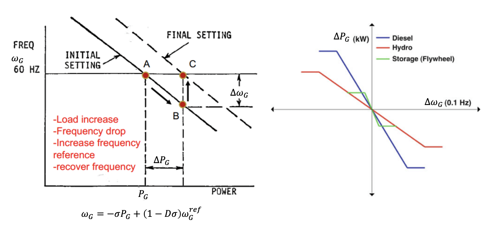
Figure 1: Basic function of secondary control: Adjusting reference set point to produce given power,assuming nominal frequency

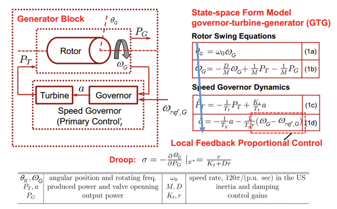
Figure 2: Sketch of a generator-turbine-governor (G-T-G) and its droop model

The actual implementation of these commands is carried out by the governor changing the set point for its “droop” $P_{G}^{ref}[K]$ in a feed-forward manner ($K$ represents the timescales relevant for tertiary control). Secondary level control is generally used to map power commands given by the tertiary level into the set points to which controllable equipment responds and/or to in a feedback manner adjust frequency set points so that incremental power is produced and the system frequency deviation within a pre-specified tolerance of $\epsilon$ is allowed. However, the line between tertiary and secondary level governor control is often gray. In systems which do not have automatic generation control (AGC), only “power sharing” commands are implemented this way. Regulation of frequency deviations resulting from relatively slow power excursions around the scheduled value is done manually in such systems. In systems with AGC, the PI governor control responding to frequency deviations, and/or area control error $(ACE)$ in multi-BA systems, adjusts the set point for governor controller $\omega_{G}^{ref}[k]$ ($k$ denotes discrete time samples relevant for secondary control) according to the three way droop relation. Shown in Figure 1 is a sketch of these droops defining relations between frequency deviations from nominal frequency $\omega_{0}$, $\Delta\omega_{G}[k]=\omega_{G}[k]-\omega_{0}$ and power increments $\Delta P_{G}[k]=P_{G}[k]-P_{G}^{ref}[K]$ for given $\omega_{G}^{ref}[k]$. AGC basically computes set point $\Delta\omega_{G}^{ref}[k]=\omega_{G}^{ref}[k+1]-\omega_{G}^{ref}[k]$ so that $\Delta\omega_{G}[k]<\epsilon$ [9]. To avoid a major confusion in recent literature concerning the notion of a droop in systems with IBRs, in particular, we point out that power sharing takes place in a feed forward way for predictable bounds on power deviations, while the AGC takes place in a feedback manner at the faster rate. Moreover, the three way droop used for AGC is a quasi-static concept which is derived by assuming that derivatives are zero as illustrated in Figure 2. The power sharing droop can be set independently in a slower feed forward way to shape the frequency response to anticipated power by the tertiary level. This clarification is written because many references in the literature assume one or the other functionality of secondary level control. There are several major issues regarding the role of secondary level control. The main is that power sharing function assumes that governor can control power generated over broad ranges of power commands given by the tertiary level. The second major issue is that the gains in governor controller are derived using a linearised turbine-generator model around pre-selected operating point. The third major issue is that secondary level assumes that primary controller stabilises and regulates output variables (frequency) to its set point, and, that it can control power generated at the right rate. All these assumptions are major causes of frequency problems in systems with intermittent resources and require further studies as discussed in Section IV.

Finally, and independent from the version of secondary control in place, a combination of primary and secondary control should guarantee that commands given by the tertiary level are implementable, namely stable, feasible and robust with respect to parameter uncertainties. In this paper we are particularly concerned with the huge issue that state-of-the-art of today’s primary controllers can generally not do this, and propose new controllers. Broadly speaking, they can not stabilise system dynamics in response to continuously varying fast power imbalances. It is generally hard to control power/rate of change of power while maintaining voltage and frequency within the operating limits. Later part of this paper describes this in some detail.

IV Structure-preserving modeling of frequency dynamics in transformed state space

In order to overcome extreme perceived complexity when attempting to improve today’s hierarchical control so that it supports the on-going changes, we propose to consider the structure-preserving modeling of electro-mechanical dynamics relevant for assessing frequency stability, briefly summarised next. Consider without loss of generality a two-area electric power system shown in Figure 3 with highly varying solar power in one of the areas.

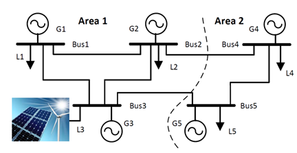
Figure 3: A sketch of two-area interconnected power system

It is known that the linearized electro-mechanical dynamics $x_{LC,i}$ of each module $i$ ( resource, load, BA, interconnected system) can be written in terms of its internal local state variables $x_{LC,i}$, and the real power exchanged with the rest of the system $P_{G,i}$. As an illustration, shown in Figure 2 is a conventional generator with its governor control. Its states $x_{LC,i}$ are shown in Figure 2, and their dynamics are

$${{\dot{x}}_{LC,i}}=\underbrace{\left[{\begin{array}[]{*{20}{c}}0&{{\omega_{0}}}&0&0\\ 0&{\frac{{{K_{d}}}}{M}}&{\frac{1}{M}}&0\\ 0&0&{-\frac{1}{{{T_{t}}}}}&{\frac{{{K_{t}}}}{{{T_{t}}}}}\\ 0&0&0&{-\frac{r}{{{T_{g}}}}}\end{array}}\right]}_{{A_{LC}}}{x_{LC,i}}+\underbrace{\left[{\begin{array}[]{*{20}{c}}0\\ {\frac{1}{M}}\\ {\;0}\\ 0\end{array}}\right]}_{{c_{M}}}{P_{G,i}}$$ (9)

It can be seen that this model takes on the standard state space form in which local state variables $x_{LC,i}=[\theta_{G,i}~{}~{}\omega_{G.i}~{}~{}P_{T,i}~{}~{}a_{i}]^{T}$ define the dynamics as a function of power generated $P_{G,i}$; notably they do not depend on $\theta_{G,i}$ explicitly [15]. Power generated and its rate of change must balance local load deviation and any other local disturbance as follows

$$\dot{P}_{G,i}=\dot{P}_{L,i}$$ (10)

When Equations (9) and (10) are combined they result in dynamical model in transformed state space of a stand alone generator $i$

$$\underbrace{\left[{\begin{array}[]{*{20}{c}}{{{\dot{x}}_{LC,i}}}\\ {{{\dot{P}}_{G,i}}}\end{array}}\right]}_{\dot{x}_{i}^{new}}=\underbrace{\left[{\begin{array}[]{*{20}{c}}{{A_{LC}}}&{{C_{M}}}\\ {{K_{P}}}&0\end{array}}\right]}_{A_{i}}x_{i}^{new}+\underbrace{\left[{\begin{array}[]{*{20}{c}}0\\ 1\end{array}}\right]}_{D_{i}}{{{\dot{P}}_{L,i}}}$$ (17)

where

$$x_{i}^{new}=[\omega_{G}~{}~{}P_{T}~{}~{}a~{}~{}P_{G}]^{T}$$ (18)

is the new state variable in transformed state space.

Consider now a BA $J,J\in\{1,2\}$ of two area system shown in Figure 3. When generators are interconnected, the model of their local states Eqn. (9) remains the same as for the stand-alone generator case and takes on the form

$$\dot{x}_{LC}=A_{LC}x_{LC}+C_{M}P_{G}$$ (19)

and the conservation of power becomes

$$\dot{P}_{G}=K_{P}\omega_{G}+\dot{F}_{e}+D_{P}\dot{P}_{L}$$ (20)

where $P_{G}$, $\omega_{G}$, $F_{e}$ and $P_{L}$ are vectors of power generated by all generators in the area, net tie-line power flow coming into the area and loads within the area [15]. Matrix $K_{P}$ is structurally singular as a direct result of conservation of energy in the area. Equations (19) and (20) combinedly result in a decentralised model of BA in transformed state space [8]

$$\left[{\begin{array}[]{*{20}{c}}{{{\dot{x}}_{LC}}}\\ {{{\dot{P}}_{G}}}\end{array}}\right]=\left[{\begin{array}[]{*{20}{c}}{{A_{LC}}}&{{C_{M}}}\\ {{K_{P}}}&0\end{array}}\right]\left[{\begin{array}[]{*{20}{c}}{{x_{LC}}}\\ {{P_{G}}}\end{array}}\right]+\left[{\begin{array}[]{*{20}{c}}0\\ {{{\dot{F}}_{e}}}\end{array}}\right]+\left[{\begin{array}[]{*{20}{c}}0\\ {{{\dot{P}}_{L}}}\end{array}}\right]$$ (31)

Once this structure is understood, it becomes fairly straightforward to formalize objectives of primary and secondary level generation control to both stabilize and regulate frequency in systems whose disturbances are continuously varying loads and/or intermittent resources. We observe that today’s separation of primary control for frequency stabilization, on one side, and secondary control for frequency regulation, on the other, can no longer be done by assuming that secondary control is quasi-static and that, as such, can be modeled using quasi-static frequency regulation droop-based models and by neglecting the grid effects [16, 17]. Instead, continuous-time models are needed to stabilize and regulate frequency in systems with ever-fluctuating power imbalances [18].

Figure 4: Emerging diverse technologies

Second, quite relevant for the changing systems is that the same structure-preserving modeling is technology agnostic; shown in Figure 4 are vastly different technologies, all of which lend themselves to the same structural modeling.

V Structure-preserving modeling of systems comprising multiple entities

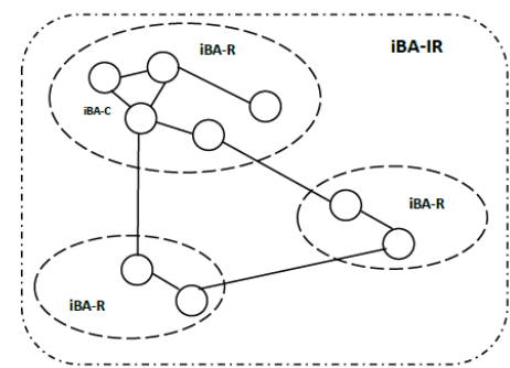
Figure 5: Emerging portfolios of intelligent Balancing Authorities (iBAs)

To further formalise modeling in the changing industry, we suggest that one of the major challenges is the lack of specifications of new technologies in terms of variables that make it possible to integrate them the same way as other resources. Shown in Figure 5 is a sketch of the emerging architectures, in which often non-utility-owned entities wish to connect to the legacy system comprising coarse BAs [19]. These new entities are “nested” within the legacy BAs, and often have their own control and decision-making “smarts”. Such emerging examples are: portfolios of wind farms and storage (See Figure 6); interconnected microgrids embedded in today’s distribution grids with and/or without own storage; clusters of EVs; neighbourhoods with controlled water pumps, HVACs, and water heaters; clusters of smart buildings; utility scale solar plants; and many more.

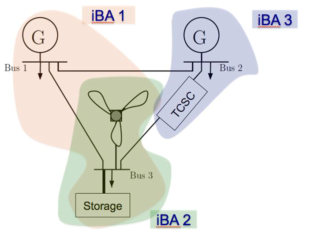
Figure 6: Emerging portfolios of intelligent Balancing Authorities (iBAs)

It is highly unrealistic to require that each of these new technologies reveals exactly their internal dynamical models and control. To overcome this problem, we propose that these enities can be viewed as technology-agnostic iBAs which can be characterized in terms of their interaction variables (intVar). This notion of intVar was introduced first for linearized systems for frequency stabilization and regulation and has two unique properties key to modeling, assessing and controlling interactions between different entities. In short, an intVar is a direct consequence of energy conservation by each iBA and, when modeling only linearized electro-mechanicial interactions can be shown to have the following [8, 9]:

• Property 1: intVar $z_{i}$ associated with component $i$ is a function of its own internal state variables written in transformed power state space, Eqn. (31)

• Property 2: When disconnected from the rest of the system it remains constant $\frac{dz_{i}}{dt}=0$.

The existence of interaction variable associated with any physical module (generator $Gi$, BA $J$) whose structure-based model in transformed state space was introduced above directly follows from the fact that its system matrix is structurally singular. For the case of BA $J$ $K_{P}$ in its transformed state space model (31) matrix $K_{P}$ is structurally singular, leading to structurally singular matrix in its transfomred state space given in Eqn. (31).

Therefore, there exists a transformation $T_{BA}$ such that

$$T_{BA}A_{BA}=0$$ (32)

where $A_{BA}$ is system matrix in BA model (31). Then, by pre-multiplying this model by such transformation it follows that

$$\dot{z}_{BA}=T_{BA}\dot{F}_{e}+T_{BA}D_{P}\dot{P}_{L}$$ (33)

The interaction variable is defined as

$$z_{BA}=T_{BA}x_{BA}^{new}$$ (34)

is the integral of power imbalance created by deviations in net tie line flow power and internal load power deviations. Similarly, it can be shown that $T_{Gi}$ exists such that

$$T_{Gi}A_{Gi}=0$$ (35)

where $A_{Gi}$ is the matrix in the generator model given in Equation (9). Its interaction variable can be shown to be

$$z_{Gi}=T_{Gi}x_{Gi}^{new}$$ (36)

The interaction variable has a straightforward physical interpretation. It is directly a result of first conservation law of energy which says that the dynamics of stored energy $E_{i}$ in a module $i$ is a result of net power injected into it $P_{i}$ minus its internal thermal loss $\frac{E_{i}}{\tau_{i}}$, as follows

$$\dot{E}_{i}=-\frac{E_{i}}{\tau_{i}}+\dot{z}_{i}$$ (37)

In the case of linearized electro-mechanical dynamics $\dot{z}_{i}=P_{i}$, where $P_{i}$ is real power out of module $i$ and $\tau_{i}$ is time constant representing thermal losses.

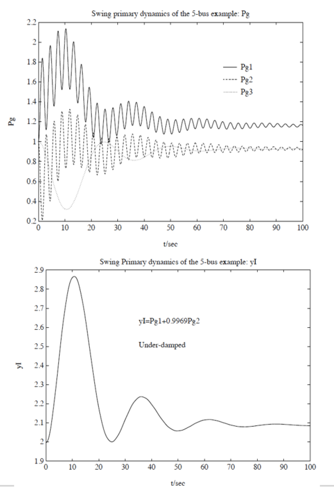
Figure 7: Interaction variables and power generated by individual plants

Shown in Figure 7 are interaction variables and internal generator power variables for the two area system shown in Figure 3 when solar power radiance is zero. Only electro-mechanical dynamics can be modeled for assessing inter-area power and frequency oscillations. We generalize the notion of intVars in Section VII that can capture the electro-magnetic fast oscillations and the effects of their inverter cotnrol.

VI Structure-based small signal frequency stability assessment

Representing small signal frequency dynamics of very large-scale multi-BA with nested iBA systems as in Figure 5, is almost an impossible task in the changing industry. The resources and loads can have very different manufacturers data, and include many diverse types, hydro, coal, gas, wind and their diverse non-standardized governor controllers. Also, many entities do not like to share their internal technology. To overcome this problem, we propose here that sources of low frequency oscillations caused by poor tuning of governors, for example, can be detected in a highly structure-preserving transparent manner by exchanging only minimal information in terms of their intVars, a method based on [20]. The method is based on conceptualising the system shown in Figure 3 as a large-scale interconnected system comprising two subsystems, shown in Figure 3. A vector Lyapunov function $v(x)=[v_{1}(x_{1})~{}v_{2}(x_{2})]^{T}$ has Lyapunov functions of each subsystem $v_{1}(x_{1})=x_{1}H_{1}x_{1}^{T}$ and $v_{2}(x_{2})=x_{2}H_{2}x_{2}^{T}$. Matrices $H_{1}$ and $H_{2}$ are computed by solving Riccati equations in each subsystem

$$A_{1}H_{1}+A_{1}^{T}H_{1} = -G_{1}$$ (38)

$$A_{2}H_{2}+A_{2}^{T}H_{2} = -G_{2}$$ (39)

where $G_{1}$ and $G_{2}$ are positive definite matrices. It can be shown that the vector Lyapunov function has negative derivative if matrix $W$ with its entries defined as

$$w_{ij} = -\frac{1}{2}\frac{\lambda_{m}(G_{i})}{\lambda_{M}(H_{i})}+\lambda_{M}^{\frac{1}{2}}(A_{ij}^{T}A_{ij})~{}~{}i=j$$ (40)

$$w_{ij} = \lambda_{M}^{\frac{1}{2}}(A_{ij}^{T}A_{ij})~{}~{}i\neq j$$ (41)

is a Metzler matrix and it is diagonally dominant [21]. Here $\lambda_{M}$ and $\lambda_{m}$ are maximum and minimum eigenvalues, respectively.

To check this condition, each subsystem computes in a decentralized manner the minimal and maximum eigenvalues and tests whether the interconnected system is made unstable because of very strong effects of interconnection matrices $A_{ij}$. This method is computationally very effective because it only requires computing extreme eigenvalues by the subsystems themselves, and checking conditions of the very low order matrix $W$ whose dimension is determined by the number of subsystems. This method, in addition to being scalable, indicates relative effects of local stability and interactions on global stability of the interconnected system. The same method can be used to design control of subsystems as well as the control of FACTS devices which can affect the strength of interactions on tie lines interconnecting subsystems. For numerical examples illustrating use of these conditions on the two area system shown in Figure 3, see [20].

VII Examples of IBR-and fault-caused electromagnetic voltage oscillations

The electro-magnetic voltage oscillations have typically been a problem during sudden fast faults in BPS. However, they are also becoming an important challenge in systems with fast fluctuating intermittent resources, due to, wind gusts and hard-to-predict variations in solar radiance. There has been a major concern about “loss of inertia” and the need for faster-responding controllers to low frequency voltage oscillations in such systems. At present there is a major effort under way to control wind and solar power fluctuations with their own fast power-electronically-switched controllers and these resources are referred to as the IBRs [22, 23]. There are also many power-electronically switched controllers placed in grid components, such as HVDC technologies, STATCOMs, Static Var Compensators (SVCs), Thyristor Controlled Series Capacitors (TCSCs) and, more recently, even electronically controlled series inductors [24].

While system planners continue to analyse likely operating problems in these newly emerging systems by relying on well-established feasibility, small signal stability and transient stability analysis tools, it is becoming increasingly clear that both enhanced modeling and new controllers are needed. The currently used software often does not even identify transient instability, and, as a result, can not assess potential benefits of deploying fast switching controllers. The industry is aware of these issues and it often resorts to using a very detailed electromagnetic transients (EMT) modeling to set and test protection during faults, for example. These tests are excessively time consuming and system-specific. Because of their complexity, they are not scalable and, most critically, can not be used to assess interactions between an IBR tested and other dynamically varying IBRs and grid controllers placed elsewhere in the system. The tests are typically done using static Thevenin equivalent of the rest of the system and applying a combination of most likely and/or most critical step power changes at the IBR location [25]. System measurements detect interactions between, for example, an IBR wind power plant and connecting weak TCSC-compensated transmission line, but there are no effective software tools for simulation of this “fighting” of IBR controllers known as control induced sub-synchronous stability (CISS) problems [4]. In this paper we propose that these oscillations caused by the IBRs and the smarts on the grid interacting can be modeled to a large extent using structure-preserving modeling described earlier in this paper by introducing a generalised interaction variable. In addition to modeling electro-mechanical stored energy the generalised energy modeling represents fast electro-magnetic dynamics as well. This is introduced in the next Section VIII. In this section we briefly illustrate the electromagnetic energy and its dependence on the controller logic used. Notably, these examples utilize TVP modeling of all components, including line currents and voltages and do not require detailed EMT modeling.

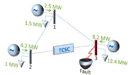
Figure 8: Fault in a BPS with small inertia wind power plant

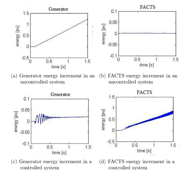
Figure 9: Dependence of electro-magnetic dynamics during faults on FACTS control: Increment of accumulated energy cause by a fault - the key role of FACTS control

Figure 10: Nonlinear control of electromagnetic energy and frequencies

Shown in Figure 8 is a sketch of a BPS with one large inertia power plant, small inertia wind power plant sending power to load via TCSC-compensated transmission line [26]. During short circuit at bus 3, load is lost and electro-mechanical energy in generators begins to increase. Prior to this, electro-magnetic energy stored in generators increases and it reduces critical clearing time determined by the electro-mechanical dynamics. Shown in Figures 9 and 10 is fast accumulated energy in the small inertia generator without TCSC, and it is contrasted with the same electro-magnetic energy transferred to the TCSC. This dynamics and the effect of fast controller cannot be modeled unless dynamics of wires and TCSC are accounted for. At the same time, it is possible to have a lumped-parameter TVP-based model for designing effective control logic without requiring excessively detailed EMT modeling. Later in Section IX we describe energy control design used here. The purpose of showing this example is to demonstrate that during fast sudden changes it becomes necessary to model electro-magnetic dynamics and not just the electro-mechanical dynamics.

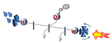
Figure 11: Small electric power grid in Flores

Shown in Figure 11 is a sketch of a small Flores power system in Azores Islands, Portugal [27].

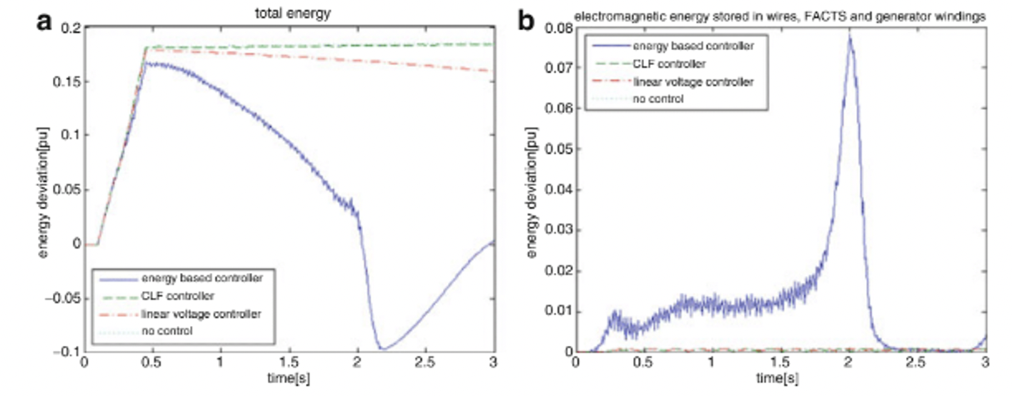
Figure 12: SVC control of short wind gust in Flores electric power grid: (a) Total accumulated energy and (b) total accumulated electromagnetic energy in a system controlled by different controller

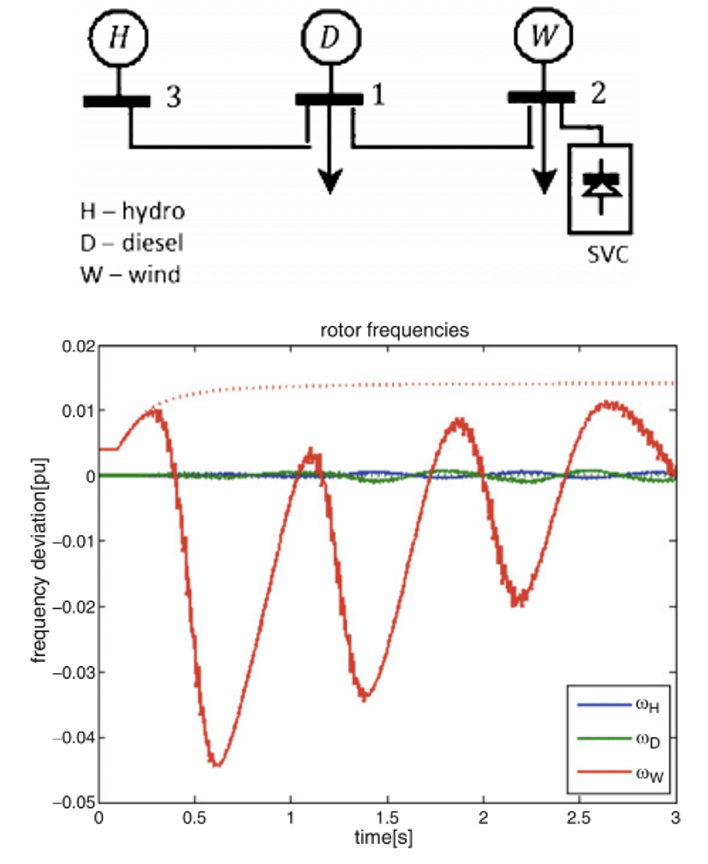
Figure 13: SVC control of short wind gust in Flores electric power grid: Mechanical frequency of all generators in the system during a short-term high- magnitude wind perturbation: (a) dashed (without control on the SVC), (b) solid (with control on the SVC)

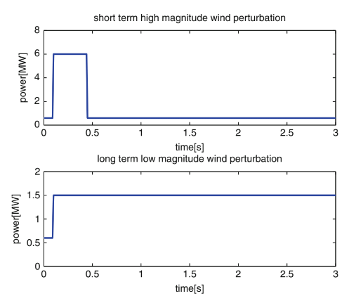
Figure 14: Long and short term wind gust in Flores electric power grid

An SVC can absorb a sudden power burst by storing electro-magnetic energy fast, as shown in Figure 12 and 13, for a sudden wind gust. A typical wind gust is shown in Figure 14 of short and long duration, respectively.

Similarly, consider a flywheel storage system connected to Flores island shown in Figure 15 (conceptual block diagram shown in Figure 16). The flywheel can compensate for a longer-duration wind gust as shown in Figure 17.

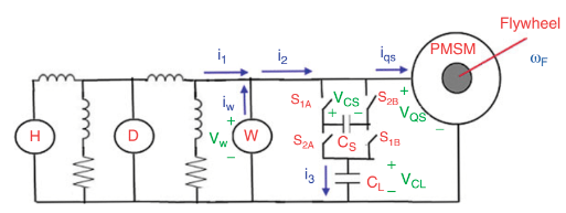
Figure 15: Full diagram connecting the flywheel to Flores

Figure 16: Interface between the power grid and the flywheel

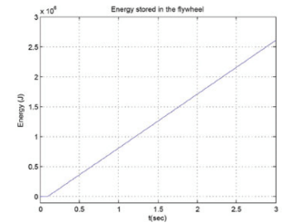
Figure 17: Flywheel control of long wind gust in Flores electric power grid

The TVP-based energy models can generally be used to design energy controllers which counteract oscillations caused by such sudden disturbances, without requiring EMT modeling. Given inherent multi-layered energy modeling in terms of interaction variables which represent the dynamics of electromagnetic interactions in addition to the dynamics of electro-mechanical interactions described in Section VI earlier in this paper, it becomes possible to control CISS problems even in large-scale changing electric power systems.

VIII Unifying structure-preserving multi-layered energy modeling

Shown in Figure 18 is a sketch of legacy system with the interconnected IBRs.The legacy system comprises conventional power plants serving slowly varying system load. The IBRs, solar in this example system, send highly fluctuating power injections and are equipped with fast power-electronically switching inverters. Shown in Figure 19 is internal design of a typical solar PV with small battery. Inverter controllers are not standardised, but for the purposes of this paper they can be thought of black boxes in which some energy is stored, and that they interact with the rest of the system by balancing energy over certain time, by balancing instantaneous power at the interconnections according to the first law of thermodynamics, conservation of energy. However, since the rates of change of instantaneous power are vastly different, it becomes necessary to also balance power at the right rates to avoid acceleration and related oscillations. It was recently proposed to generalize the interaction variable previously used for assessing and controlling electro-mechanical dynamics, as described in the section above.

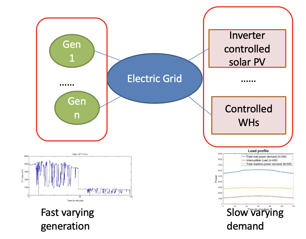
Figure 18: IBRs interconnected to a legacy BPS; fast IBR generation serving slow system load

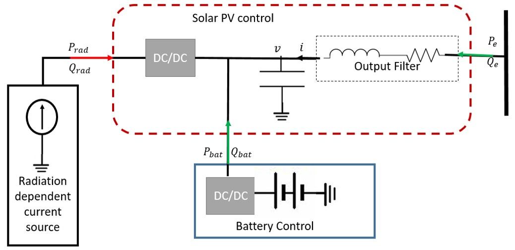
Figure 19: Internal design of a typical solar PV with a battery

Such generalized interaction variable is defined as [28, 29].

$$\dot{z}^{out}_{i}=[P^{out}_{i}~{}~{}\dot{Q}^{out}_{i}]^{T}$$ (42)

It has the same structural properties as the interaction variable characterizing electro-mechanical dynamics introduced above in Eqn. (37), except that it depends on both its states and rates of change of internal states. As such, it is instrumental in modeling interactions between different modules without making decoupling assumptions or having to linearize nonlinear models. In particular, it was shown that the dynamics of aggregate variables, both energy $E_{i}$ and its rate of change $p_{i}=\frac{dE_{i}}{dt}$ take on a general technology-agnostic form

$$\dot{E}_{i} = -\frac{E_{i}}{\tau_{i}}+P^{out}_{i}+P^{u}_{i}=p_{i}$$ (43)

$$\dot{p}_{i} = 4E_{t,i}-\dot{Q}^{out}_{i}-\dot{Q}^{u}_{i}$$ (44)

The interaction variables must obey both conservation of instantaneous power and the rate of change of generalized instantaneous power. Basically, both instantaneous power out of module $i$ and rate of change of instantaneous reactive power should balance with the net instantaneous power and the net rate of change of instantaneous reactive power being sent from the neighbouring modules, respectively, as follows

$$P^{out}_{i} = P^{in}_{j}$$ (45)

$$\dot{Q}^{out}_{i} = \dot{Q}^{in}_{j}$$ (46)

The aggregate interactive model defining rate of change of energy and rate of change of reactive power is given in Eqn. (43) and (44) and is subject to conservation laws of rate of change of interaction variable defined in Eqn. (Eqn. 42) as in Eqn. (45) and Eqn. (46).

VIII-A An example of structure preserving solar PV serving constant power load

Shown in Figure 20 is a conceptual sketch of solar PV with a battery [30]. Internal states are inductor current and capacitor voltage and inverter-controlled solar source is shown as a controllable DC source. There are several different ways of controlling this source, ranging from two-loop proportional voltage-current controller; or PID controller; or energy based control which stabilizes aggregate variables by aligning the interaction variables between the solar PV and power load.

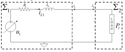
Figure 20: Sketch of an inverter controlled solar battery serving power load

In Section IX we will describe in detail the effects of primary controllers on closed loop dynamics of inverter-controlled solar PV with a battery. For purposes of illustrating further energy modeling and control we consider without loss of generality its representation as a voltage controlled source connected via RL circuit, with the objective of serving constant power load as shown in Fig. 21.

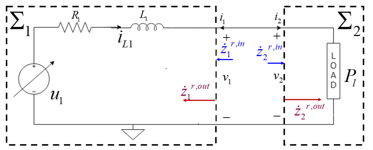
Figure 21: Interconnected system comprising interactions between RLC circuit with controllable voltage source ($\Sigma_{1}$) and a load with given power specifications ($\Sigma_{2}$)

This circuit can be thought of as comprising two interacting modules $\Sigma_{1}$ and $\Sigma_{2}$ . The dynamics of internal state variable, inductor current, takes on the form

$$\frac{di_{L1}}{dt}=-\frac{R_{1}}{L_{1}}i_{L1}+\frac{1}{L_{1}}u_{1}-\frac{1}{L_{1}}v_{1}$$ (47)

Its energy model takes on the form

$$\dot{E}_{1} = -\frac{E_{1}}{\tau_{1}}+P^{out}_{1}+P^{u}_{1}$$ (48)

$$\dot{p}_{1} = 4E_{t,1}-\dot{Q}^{out}_{1}+\dot{Q}^{u}_{1}$$ (49)

where $E_{1}=\frac{1}{2}Li_{L1}^{2}$, $\frac{E_{1}}{\tau_{1}}=Ri_{L1}^{2}$, $P^{u}_{1}$ and $\dot{Q}^{u}_{1}$ are interaction variables between the controllable source and the RL circuit within the module $\Sigma_{1}$. The term $E_{t,1}=\frac{1}{2}L(\frac{di}{dt})^{2}$ is the stored energy in tangent space. The aggregate variables of this module are $x_{z,1}=[E_{1}~{}~{}p_{1}]^{T}$, and their dynamics takes on the form

$$\dot{x}_{z,1}=A_{z,1}x_{z,1}+B_{z}u_{z,1}+B_{t}E_{t,1}+B_{z}\dot{z}_{1}^{out}$$ (50)

Here, $B_{t}=\left[0,4\right]^{T},B_{z}=\left[1,-1\right]^{T}$ for any component and matrix $A_{z,1}=\left[{\begin{array}[]{*{20}{c}}{-1/{\tau_{1}}}&0\\ 0&0\end{array}}\right]$ depend only on the time constant $\tau_{1}$.

Notably, when aggregate control is selected to be $u_{z,1}=[P^{u}_{1}~{}~{}\dot{Q}^{u}_{1}]^{T}$, it can be designed to align the rate of change of interaction variable $\dot{z}_{1}^{out}$ and rate of change of interaction variable $\dot{z}_{2}^{out}$ from $\Sigma_{2}$. The closed loop aggregate dynamics is linear and can be shaped in a provable manner. This control design is illustrated next.

IX Unifying energy control of interaction dynamics

It follows from the above derivations that a technology-agnostic energy controller which aligns rate of change of interaction variables so that the conservation of power and rate of change of reactive power are observed according to Eqns. (45) and (46). This is achieved by having the control in energy space $u_{z,1}$ respond to the the output variable that takes the form

$$y_{z,1}=C_{t,1}E_{t,1}+C_{z,1}x_{z,1}+D_{z,1}(\dot{z}^{out}_{1}-\dot{z}_{1}^{ref})$$ (51)

where $\dot{z}_{1}^{ref}=\dot{z}_{2}^{out}$. The energy control can be designed to both cancel error dynamics and the term $E_{t,1}$. Alternatively, the term $E_{t,1}$ can be upper-bounded and the sliding mode control implementation can be done [30].

This technology-agnostic control $u_{z,1}$ needs to be mapped into physically-implementable control signal. In the case of $\Sigma_{1}$ the physical control signal is $u_{1}=v_{1}$. The implementation of this physical control signal is typically power-electronically controlled switch. This map is non-unique and one example of mapping is shown in Eqn. (52) resulting in a dynamical control.

$$\frac{du_{1}}{dt}=\frac{u_{1}}{i_{L1}}\frac{di_{L1}}{dt}-\frac{\dot{Q}_{1}^{u}}{i_{L1}}$$ (52)

IX-A Dependence of system response on controller logic when serving constant power load

As one attempts to control systems with IBRs, it is necessary to assess performance of today’s state-of-the-art controllers with the energy controllers described in this paper. The actual expression for energy control differs depending on whether the objective is to:

• Single timescale energy control: Align power controlled by the IBR after its stored energy settles.

• Two timescale energy control: Align both instantaneous power and rate of change of instantaneous reactive power controlled by the IBR and required by the load.

To illustrate this, consider without loss of generality a step power change required by the load from the IBR sketched in Figure 20. This scenario is rather difficult because constant power load is known to create negative incremental resistance problem which inherently leads to voltage collapse and/or other types of unacceptable dynamics in IBRs controlled by conventional controllers. Shown in Figure 22(a) is the response of such controller. It can be seen that typically-used two loops control will have problems serving constant power load as shown in Figure 22(a), voltage collapsing after several seconds. To the contrary, the response of a conventional proportional-derivative (PD) controller remain stable, as shown in the plots in Figure 22(b). This plot highlight the key relevance of dynamic controllers.

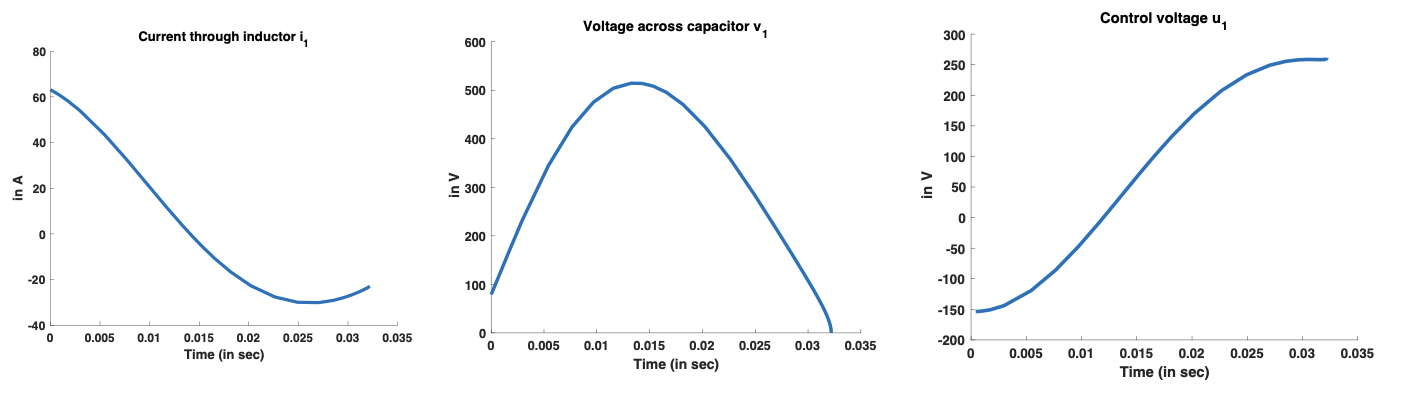
(a) PI two loop controller resulting in voltage collapse

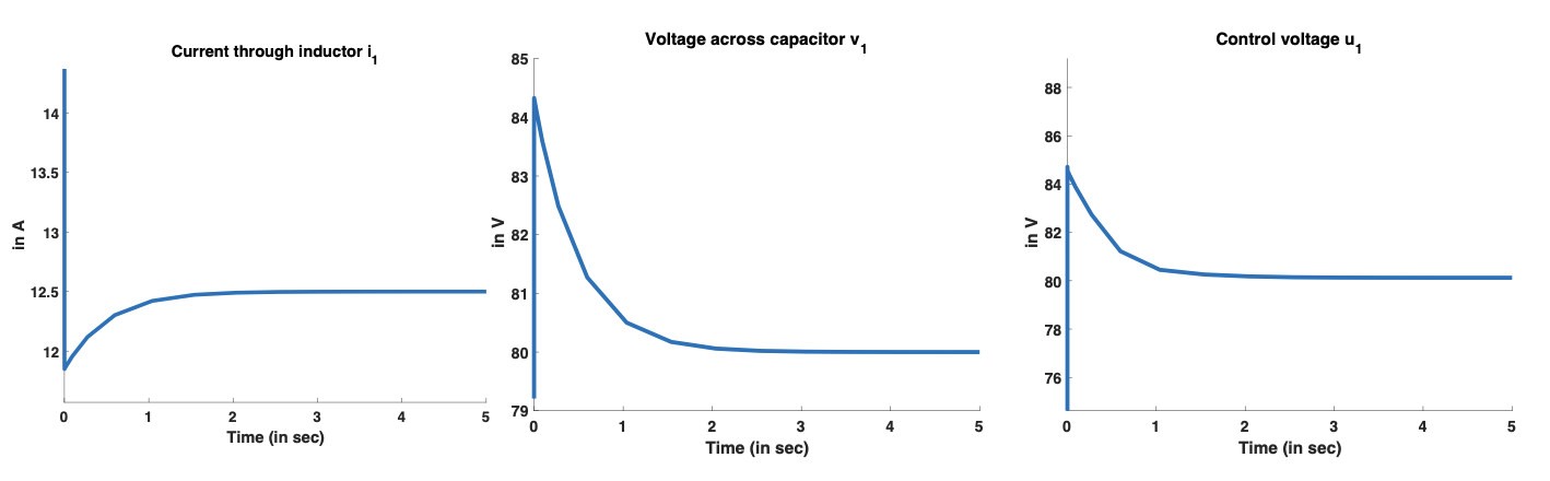
(b) PD controller resulting in stable response

Figure 22: Closed loop response to step power load change

.

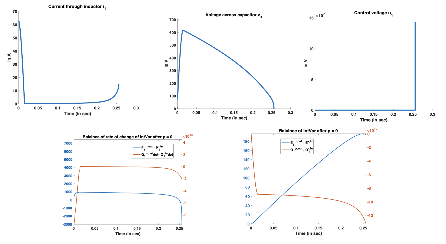
Figure 23: Closed loop response to step power load change: Single timescale nonlinear energy controller; Upper plots show the state trajectories. Lower plots show the evolution of the difference in the outgoing and incoming interaction variables.

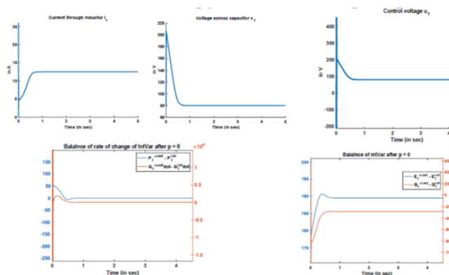
Figure 24: Closed loop response to step power load change: Two-timescale nonlinear energy controller; Lower plots show the evolution of the difference in the outgoing and incoming interaction variables.

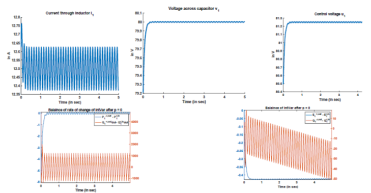
Figure 25: Closed loop response to small intermittent fluctuations: Conventional feedback control

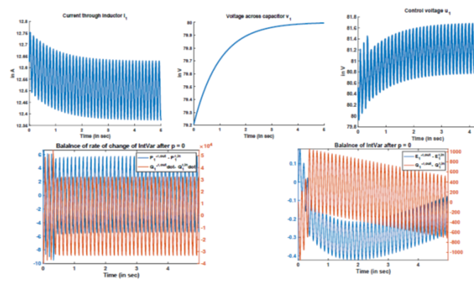
Figure 26: Closed loop response to small intermittent fluctuations: Constant gain derivative control responding to voltage

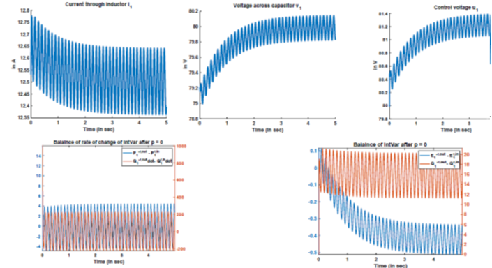
Figure 27: Closed loop response to small intermittent fluctuations: Single timescale nonlinear energy controller; Lower plots show the evolution of the difference in the outgoing and incoming interaction variables.

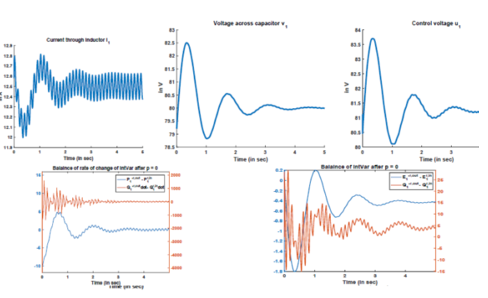
Figure 28: Closed loop response to small intermittent fluctuations: Two-timescale nonlinear energy controller; Lower plots show the evolution of the difference in the outgoing and incoming interaction variables.

Shown next in Figure 23 is the closed loop dynamic response for the same scenario with the energy controllers when both electro-mechanical and electro-magnetic dynamics are controlled as a single time scale process, and when the only control objective is to alignment of instantaneous power after energy dynamics settles ($\frac{dE}{dt}=0$). It can be seen that even this nonlinear controller is not fast enough to stabilize system response and to avoid voltage collapse.

However, when the energy controller is designed with the objective to align both instantaneous power and rate of change of instantaneous reactive power at the interfaces of IBR and constant power load, and time scale separation between these processes is carefully accounted for by using slow reduced order model to stabilise electro-mechanical dynamics and fast reduced order model is used to stabilise fast reactive power rate of change, shown in Figure 24 is closed loop stable response.

IX-B Dependence of system response on controller logic when serving intermittent power load

A similar comparison of the effects of iBR controllers on closed loop response can be shown in response to fluctuating power disturbances seen by the IBR. Shown in Figure 25 is the closed loop response to small intermittent fluctuations. It can be seen that conventional feedback is too slow to cancel the fast imbalances, resulting in small persistent oscillations in voltage. The response obtained with dynamical PD controller cancels the persistent oscillations, but results in slower response as shown in Fig. 26.

The response obtained with single timescale energy control is shown in Fig. 27. It can be seen that even this nonlinear controller is not able to suppress fast imbalances. Finally, the responses obtained with two timescale energy control is shown in Fig. 28, which results in perfect voltage regulation. We further see that the instantaneous and reactive power imbalances settle at zero.

X Concluding recommendations: Structure-preserving standards/protocols for reliable and efficient multi-energy systems

In closing, this paper takes a broad look at the state-of-the-art hierarchical modeling and control for bulk power systems. It identifies several hidden roadblocks to using this paradigm in support of large-scale decarbonization. Fundamental challenges are described first. It is proposed next to utilize structure-preserving modeling of complex power grids which has been introduced by our many collaborators and former doctoral students both at Carnegie Mellon University and, more recently at M.I.T. These concepts are explained in the context of emerging low frequency oscillations, using the notion of interaction variable. Then a recent generalization of interaction variables is introduced and it is suggested that energy modeling which captures both instantaneous power and instantaneous rate of change of reactive power be considered as the basis for multi-layered modeling of the changing electric energy systems. An aggregate model of technology-agnostic module is derived in terms of stored energy and its rate of change, and it is used for nonlinear energy control. A proof-of-concept energy control which avoids voltage collapse and significantly reduces otherwise persistent oscillations created by intermittent IBRs is presented using a DC voltage controlled source which supplies time varying power. Based on these findings, further research is needed toward a modular feed-forward distributed information exchange in support of self-adaptation of subsystems to ensure feasible interconnected system.

We propose the interaction-based energy modeling to be used as the basis for structure preserving interacting standards/protocols that ensure stable operations in the changing systems comprising multiple layers of intelligent Balancing Authorities (iBAs) with well-defined interfaces to the rest of the system. We suggest three steps toward generalising today’s area control error (ACE) as the basis for reliable and efficient emerging systems operation. They are as follows:

• Generalise today’s coarse balancing authorities into intelligent Balancing Authorities (iBAs).

• Enhance today’s AGC standard Area control error (ACE) into generalized interaction variables as the measure of any iBAs performance.

• Work toward next generation end-to-end SCADA supported by the information exchange proposed.

These three steps form the foundations of interactive operations in future energy systems so that they can be modelled, controlled and operated without excessive complexity.

References

- [1] J. Wyatt and M. Ilic, “Time-domain reactive power concepts for nonlinear, nonsinusoidal or nonperiodic networks,” in IEEE international symposium on circuits and systems. IEEE, 1990, pp. 387–390.
- [2] “Performance-based energy resource feedback, optimization, and risk management,” https://arpa-e.energy.gov/technologies/programs/perform, accessed: 2022-05-11.
- [3] K. Uhlen, S. Elenius, I. Norheim, J. Jyrinsalo, J. Elovaara, and E. Lakervi, “Application of linear analysis for stability improvements in the nordic power transmission system,” in 2003 IEEE Power Engineering Society General Meeting (IEEE Cat. No. 03CH37491), vol. 4. IEEE, 2003, pp. 2097–2103.
- [4] J. Adams, V. A. Pappu, and A. Dixit, “Ercot experience screening for sub-synchronous control interaction in the vicinity of series capacitor banks,” in 2012 IEEE Power and Energy Society General Meeting. IEEE, 2012, pp. 1–5.
- [5] M. J. Hossain, H. R. Pota, M. A. Mahmud, and R. A. Ramos, “Investigation of the impacts of large-scale wind power penetration on the angle and voltage stability of power systems,” IEEE Systems journal, vol. 6, no. 1, pp. 76–84, 2011.
- [6] F. Li, A. Z. Liu, and G. R. Swenson, “Characteristics of instabilities in the mesopause region over maui, hawaii,” Journal of Geophysical Research: Atmospheres, vol. 110, no. D9, 2005.
- [7] E. Troester, “New german grid codes for connecting pv systems to the medium voltage power grid,” in 2nd International workshop on concentrating photovoltaic power plants: optical design, production, grid connection, 2009, pp. 1–4.
- [8] M. D. Ilić and S. Liu, Hierarchical power systems control: its value in a changing industry. Springer, 1996.
- [9] M. D. Ilic and J. Zaborszky, Dynamics and control of large electric power systems. Wiley New York, 2000.
- [10] S. Cvijić, M. Ilić, E. Allen, and J. Lang, “Using extended ac optimal power flow for effective decision making,” in 2018 IEEE PES Innovative Smart Grid Technologies Conference Europe (ISGT-Europe). IEEE, 2018, pp. 1–6.
- [11] M. Ilic and J. Lang, “Final report entitled voltage dispatch and pricing in support of efficient real power dispatch,” 2012.
- [12] M. Ilic, R. S. Ulerio, E. Corbett, E. Austin, M. Shatz, and E. Limpaecher, “A framework for evaluating electric power grid improvements in puerto rico,” 2020.
- [13] A. Nejat, L. Solitare, E. Pettitt, and H. Mohsenian-Rad, “Equitable community resilience: The case of winter storm uri in texas,” arXiv preprint arXiv:2201.06652, 2022.
- [14] M. Ilic, R. Jaddivada, X. Miao, and N. Popli, “Toward multi-layered mpc for complex electric energy systems,” in Handbook of Model Predictive Control. Springer, 2019, pp. 625–663.
- [15] M. Ilic and X. Liu, “A simple structural apporach to modeling and control of the inter-area dynamics of the large electric pwoer systems: Part ii nonlinear models of frequency and voltage dynamics,” in Proceedings of the North American Power Conference (NAPS) IEEE, 1994.
- [16] M. Ilic, X. Liu, B. Eidson, C. Vialas, and M. Athans, “A structure-based modeling and control of electric power systems,” Automatica, vol. 33, no. 4, pp. 515–531, 1997.
- [17] P. S. Kundur, N. J. Balu, and M. G. Lauby, “Power system dynamics and stability,” Power system stability and control, vol. 3, 2017.
- [18] M. D. Ilić and Q. Liu, “Toward sensing, communications and control architectures for frequency regulation in systems with highly variable resources,” in Control and optimization methods for electric smart grids. Springer, 2012, pp. 3–33.
- [19] M. D. Ilić, “Dynamic monitoring and decision systems for enabling sustainable energy services,” Proceedings of the IEEE, vol. 99, no. 1, pp. 58–79, 2010.
- [20] Q. Liu, “Large-scale systems framework for coordinated frequency control of electric power systems,” Ph.D. dissertation, Carnegie Mellon University, 2013.
- [21] A. Zecevic and D. D. Siljak, Control of complex systems: Structural constraints and uncertainty. Springer Science & Business Media, 2010.
- [22] M. Ilic and et. al, “Ieee tf report on pes simulation methods, models, and analysis techniques to represent the behavior of bulk power system connected inverter-based resources,” (Under Preparation) 2022.
- [23] Y. Lin, J. H. Eto, B. B. Johnson, J. D. Flicker, R. H. Lasseter, H. N. Villegas Pico, G.-S. Seo, B. J. Pierre, and A. Ellis, “Research roadmap on grid-forming inverters,” National Renewable Energy Lab.(NREL), Golden, CO (United States), Tech. Rep., 2020.
- [24] “Smart wires - reimagine the grid,” https://www.smartwires.com/, accessed: 2022-05-11.
- [25] P. Godin, M. Fischer, H. Röttgers, A. Mendonca, and S. Engelken, “Wind power plant level testing of inertial response with optimised recovery behaviour,” IET Renewable Power Generation, vol. 13, no. 5, pp. 676–683, 2019.
- [26] M. Cvetković and M. D. Ilić, “Ectropy-based nonlinear control of facts for transient stabilization,” IEEE Transactions on Power Systems, vol. 29, no. 6, pp. 3012–3020, 2014.
- [27] M. Ilic, L. Xie, and Q. Liu, Engineering IT-enabled sustainable electricity services: the tale of two low-cost green Azores Islands. Springer Science & Business Media, 2013, vol. 30.
- [28] M. D. Ilić and R. Jaddivada, “Multi-layered interactive energy space modeling for near-optimal electrification of terrestrial, shipboard and aircraft systems,” Annual Reviews in Control, vol. 45, pp. 52–75, 2018.
- [29] M. D. Ilic and R. Jaddivada, “Fundamental modeling and conditions for realizable and efficient energy systems,” in 2018 IEEE Conference on Decision and Control (CDC). IEEE, 2018, pp. 5694–5701.
- [30] R. Jaddivada and M. D. Ilic, “A feasible and stable distributed interactive control design in energy state space,” in 2021 60th IEEE Conference on Decision and Control (CDC). IEEE, 2021, pp. 4950–4957.