PerfCE: Performance Debugging on Databases with Chaos Engineering-Enhanced Causality Analysis

Abstract

Debugging performance anomalies in databases is challenging. Causal inference techniques enable qualitative and quantitative root cause analysis of performance downgrades. Nevertheless, causality analysis is challenging in practice, particularly due to limited observability. Recently, chaos engineering (CE) has been applied to test complex software systems. CE frameworks mutate chaos variables to inject catastrophic events (e.g., network slowdowns) to stress-test these software systems. The systems under chaos stress are then tested (e.g., via differential testing) to check if they retain normal functionality, such as returning correct SQL query outputs even under stress.

To date, CE is mainly employed to aid software testing. This paper identifies the novel usage of CE in diagnosing performance anomalies in databases. Our framework, PerfCE, has two phases — offline and online. The offline phase learns statistical models of a database using both passive observations and proactive chaos experiments. The online phase diagnoses the root cause of performance anomalies from both qualitative and quantitative aspects on-the-fly. In evaluation, PerfCE outperformed previous works on synthetic datasets and is highly accurate and moderately expensive when analyzing real-world (distributed) databases like MySQL and TiDB.

I Introduction

Databases are critical infrastructures that support daily operations and businesses. Service outages or performance defects can result in a negative user experience, a decline in sales, and even brand damage. Google, for instance, assesses page speed for ranking websites [1]. According to reports, every 100ms of latency costs Amazon 1% in revenue [2], and every 0.5s of additional load delay for Google search results leads to a 20% loss in traffic [3]. Modern databases often entail complex resource management, and dependencies between modules of a (distributed) database may introduce subtle performance bottlenecks and degrade system throughput. Diagnosing performance issues is cumbersome and error-prone, especially as typical (distributed) databases on the cloud or containerization environments may be exposed to hundreds of potentially influencing key performance indicators (KPIs).

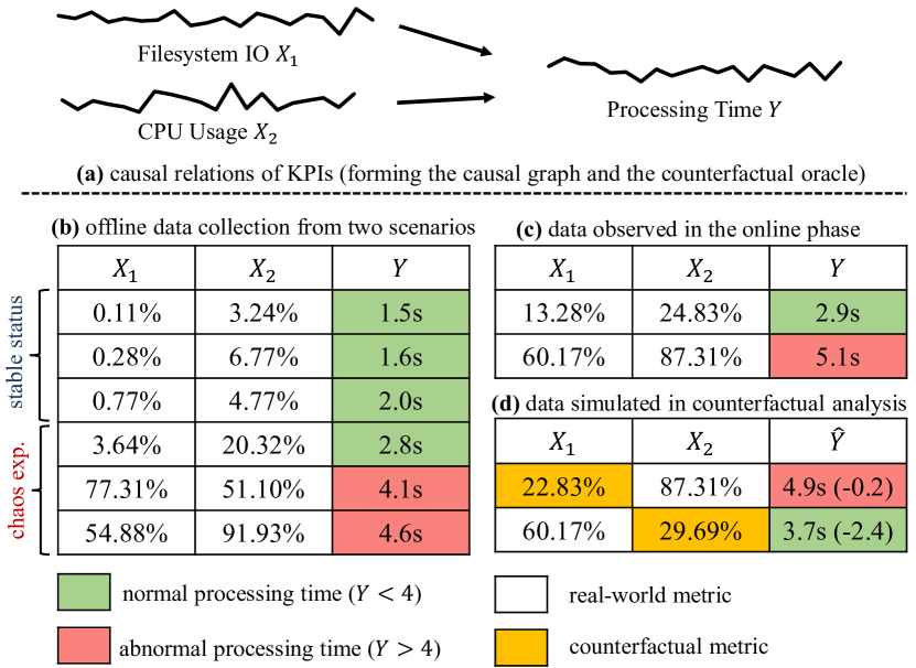
Figure 1: Motivating example of performance debugging.

Usage Scenario. Considering Fig. 1, which contains three KPIs. Filesystem IO $X_{1}$ and CPU usage $X_{2}$, as two causes, influence the database query processing time $Y$. A developer, Bob, observes a processing time spike (5.1s) and wonders the root cause of this spike. He manually checks all performance metrics and identifies that the spike is due to high CPU usage.

Ideal Solution. As disclosed by vendors [4], a burst of performance anomalies may last only a few minutes, whereas human-intensive diagnoses can take much longer. Causal graphs are an automated and interpretable solution to this problem, providing informative causal relations among variables [5]. In this context, Bob would use the causal graph and a counterfactual oracle, derived from KPI causal relations, to diagnose performance issues. Bob would first identify all ancestors of the node indicating processing time $Y$ by traversing the causal graph (see Fig. 1(a)). These ancestors represent direct or indirect causes of performance downgrades. Bob would then submit counterfactual queries to the oracle to determine whether a particular cause, when changed to a given extent, could resolve the performance downgrade. The root cause would be the counterfactual change that fixes the performance downgrade. For example, in Fig. 1(d), Bob submits two counterfactual queries (yellow cells) to the oracle and receives $\hat{Y}$ after such counterfactual changes. Bob observes that when $X_{1}$ (filesystem IO) resumes normal operations, processing time $\hat{Y}$ remains elevated (1st row in Fig. 1(d)). When $X_{2}$ (CPU usage) drops to its mean value, $\hat{Y}$ returns to normal (2nd row in Fig. 1(d)). Thus, Bob attributes this spike to high CPU usage.

Challenge. Establishing causal graphs and counterfactual oracles is a long-standing challenge in causality analysis. Existing works use off-the-shelf causal discovery algorithms [6, 7, 8] or hand-coded rules [5, 9] to identify causal graphs from observational data. A predictive model is then trained on causal relations to support counterfactual analysis. However, they are insufficient for systematic performance diagnosis due to limited observability [10]. Performance downgrades are rare, so the causal graph learned from mostly normal states may be biased and unsuitable for analyzing performance downgrades. Additionally, the predictive model rarely considers confounders, leading to erroneous counterfactual predictions [11, 12].

Our Approach. We adopt chaos engineering (CE) to address the aforementioned challenge. CE is an emerging engineering practice which extensively injects faults (e.g., network slowdowns) into a system to assess its reliability. To overcome limited observability, we employ CE to stress various system events, thus creating sufficient and authentic abnormal data. This enables us to learn high-quality causal graphs and oracles. These are shown in the “chaos exp.” rows in Fig. 1(b).

Overall, we present PerfCE, a CE-enhanced causal analysis framework for performance debugging. PerfCE consists of two phases: offline and online. In the offline phase, besides passive observations, CE enables us to actively collect abnormal data (i.e., those “chaos exp.” rows in Fig. 1(b)); we can thus learn an accurate and comprehensive causal graph. Moreover, we use CE to actively mutate chaos variables (a CE framework typically offers multiple chaos variables, where mutating each chaos variable can influence hundreds of KPIs), delivering an accurate estimation of structural equation models (SEMs). We incorporates a set of design principles and optimizations to overcome challenges (e.g., confounders) in the offline phase.

In the online phase, when a performance anomaly is observed (Fig. 1(c)), we collect the ancestors of the processing time $Y$ on the causal graph (Fig. 1(a)) to scope possible root cause KPIs. Moreover, we use the SEM to issue qualitative counterfactual queries and obtain accurate root cause analysis, e.g., identifying CPU usage $X_{2}$ as the root cause of the anomaly in Fig. 1(d).

Main Results. PerfCE uses an industrial-strength chaos framework, Chaos Mesh [13], to establish causal graphs and SEMs with high quality. Evaluation using synthetic datasets shows that PerfCE offers highly accurate causality analysis. Moreover, we evaluate PerfCE using MySQL and a distributed database TiDB [14] on the Kubernetes (K8s) [15] container environments. Human evaluation show that PerfCE can reliably diagnose performance defects incurred by various system resources, outperforming existing works with reasonable cost. In summary, we make the following contributions:

• We for the first time advocate using CE for causality analysis-based performance diagnose. Modern CE frameworks, in its “out-of-the-box” manner, principally addresses the low observability issue in causal analysis.

• We design PerfCE to conduct automated performance anomaly diagnosis for complex (distributed) databases. PerfCE incorporates a set of design principles and optimizations to enable qualitative root cause identification and quantitative counterfactual analysis. We (anonymously) release our codebase at [16] and maintain a documentation at [17] to help practitioners use PerfCE.

• We evaluate PerfCE on synthetic datasets and real-world (distributed) databases. PerfCE shows superior performance over prior works with moderate cost.

II Preliminary

II-A Database Performance Diagnosis

Database developers and users, when encountering performance anomalies, often aim to identify relevant information for debugging. We classify performance debugging into two categories based on the available information:

Blackbox Debugging: Localizing KPIs. Database performance downgrades are often due to abnormal system components like kernel, network, or pod failures in container clusters [18]. In blackbox debugging, users identify root cause KPIs without accessing database internals. For instance, a developer might want to determine the cause of an intermittently slow SQL query [4], ultimately finding KPIs like high CPU usage or low disk throughput. Blackbox debugging is challenging: databases often consist of numerous KPIs (e.g., our evaluated cases have up to 254 KPIs; see Sec. V), making it difficult to identify root cause KPIs. Statistical debugging (SD) [19, 20, 21] can find KPIs correlated to anomalies, but correlation does not imply causation, limiting SD’s applicability and accuracy. A promising approach is using causality analysis [5, 6] to establish causal relations between KPIs, recasting the identification of root cause KPIs as predicting KPIs with major causation with anomalies based on the causality graph.

Whitebox Debugging: Localizing Program Bugs. Software bugs may also cause performance anomalies. This scenario assumes that programmers can monitor software internals, with typical approaches including software profiling [22, 23], visualization [24], and program analysis techniques like program slicing [25], delta debugging, and statistical debugging [19, 20, 21, 26, 27]. The end goal is often to isolate buggy code representing performance bottlenecks.

Focus of This Work. Our focus is orthogonal to existing whitebox debugging tools that aim to find database bugs [28, 29, 30]. That is, we perform blackbox debugging to localize KPIs that result in the performance anomalies. PerfCE provides a CE-enhanced causal analysis framework for blackbox debugging, and it is agnostic to specific database implementation. We now introduce preliminaries of causal analysis and CE.

II-B Causality Analysis

Qualitative Causality Analysis. Identifying root causes of performance anomalies in Fig. 1, such as abnormal CPU usage leading to processing time spike, requires a qualitative approach using causality analysis. This process flags one or multiple KPIs considered as the root causes of performance defects and requires a causal graph, defined as follows:

Definition 1 (Causal Graph).

A causal graph (Bayesian network) is a directed acyclic graph (DAG): $G=(V,E)$. Each node $X$ represents a random variable, and each edge $X\to Y$ encodes their cause-effect relationships, with $X$ being a direct cause of $Y$. $Pa_{G}(X)$ denotes the parent nodes of $X$ in $G$.

Using causal graphs, identifying anomaly root causes involves determining cause-effect relations between graph ancestors and descendants. Given an abnormal KPI $Y$, a common approach backtracks its ancestors and identifies the most ancestral abnormal KPI $X_{i}$ as the root cause [6].

Quantitative Causality Analysis. As discussed in Sec. I, performance anomaly root cause analysis needs a quantitative perspective of causal relations, typically enabled by counterfactual analysis using a structural equation model (SEM) [31] on a qualitative causal graph.

Definition 2 (SEM).

A SEM $M$ consists of:

1. Exogenous variables $U$, representing factors outside the model;

2. Observed endogenous variables $V$, with each variable $X$ functionally dependent on $U_{X}\cup Pa_{G}(X)$, where $U_{X}\subseteq U$.

3. Deterministic functions $f_{X}\in F$, each $f_{X}:Pa_{G}(X)\times U_{X}\to X$ computing the value of $X$.

Average treatment effect (ATE) [32] quantifies the counterfactual causal effect of treatment $X$ on outcome variable $Y$ in counterfactual analysis, which answers counterfactual queries:

$$\text{ATE}=\mathbb{E}[Y\mid do(X=\bm{x}_{1})]-\mathbb{E}[Y\mid do(X=\bm{x}_{2})]$$ (1)

Here, $do(\cdot)$ represents an intervention on variable $X$. Intervention sets a variable to a constant value, making it independent of its parents. The example above asks, ”what would $Y$ change if $X$ were $x_{1}$ instead of $x_{2}$?” Counterfactual queries like $do(X=x)$ simulate interventions by removing edges between $X$ and its parent nodes in the SEM, replacing $X$ with a constant $X=x$, while keeping other causal relations unchanged [33, 34]. However, the SEM is unknown in practice, requiring SEM learning from data and recasting the ATE causal semantics into a statistical estimand. Computing ATE is challenging when parent variables interact or are unmeasured in the causal graph. Our solutions in Sec. IV-A address such challenges and generalize to complex causal graphs.

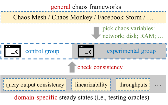
Figure 2: Using CE to aid software testing.

II-C Chaos Engineering (CE)

As large-scale, distributed systems evolve, traditional software testing methods become less effective. CE tests a system’s ability to withstand turbulent conditions in production [35]. In cloud/container environments, turbulence may include infrastructure, pod, network, and application failures. Fig. 2 shows how CE can be used to aid software testing. In general, CE typically involves three steps:

(I) Defining Steady State. CE starts by defining test oracles, or “steady states,” as easily measurable outputs of a system that indicate normal behavior. The key hypothesis is that a steady state will persist in both a control group and the experimental group subjected to CE stress.

Steady states may include throughput and query outputs, considering domain-specific demands. For example, SQLSmith [36] compares the outputs of a database (under CE stress) and MySQL. The steady state is defined as the SQL execution outputs being consistent between the two databases. This setup expands the standard “differential testing” procedure [37, 38, 39], requiring consistency between the experimental group and reference even under CE stress.

(II) Picking Chaos Variables. CE consists of chaos variables, each representing a critical, low-level factor that may induce failures in infrastructure, networks, and systems. Modern CE frameworks like Chaos Mesh [13] are coupled with containerization environments like K8s. offering chaos variables for various failures in K8s clusters (e.g., container-kill, pod-kill). Chaos variables are not the same as KPIs; there are usually more KPIs than chaos variables. Mutating each chaos variable (e.g., an IO-related variable) may affect many KPIs (e.g., average I/O time).

(III) Launching CE and Testing. After (I) and (II), CE can be launched to test the target system, checking for inconsistencies between the reference group and the target system (experimental group) under CE. Findings can be used for debugging and error fixing.

III Motivation, Related Work and Overview

This section discusses the key technical challenges of causality analysis and reviews existing works. We then illustrate the synergistic effect of integrating causality analysis with CE.

Challenges in Rule-Based Causality Analysis. Existing causal-based performance debugging can be categorized into rule-based construction and learning-based construction. However, the accuracy of estimated causal graphs by both methods remains questionable. First, rule-based construction is highly dependent on expert knowledge and is human-intensive, which may not always be correct with respect to the rigorous mathematical properties of causal relationships [10]. In fact, rule-based methods usually aim at a specific application with limited types of metrics; e.g., Sage [5], one state-of-the-art work, only supports latency-related KPIs.

Challenges in Learning-Based Causality Analysis. Rule-based constructions require domain-specific knowledge (e.g., microservice topological structures) and can only be applied to some specific types of KPIs (e.g., Sage is only applicable for latency-related KPIs) [5]. In contrast, learning-based causality construction is generally of higher applicability than rule-based methods. Recent works [8, 6, 7] use learning-based approaches to create causal graphs for performance debugging. This allows for more flexible causal inference with broader applications. Nevertheless, in performance debugging, it is challenging to construct SEMs for qualitative/quantitative causality analysis. The key issue is the limited observability. Overall, data collected during normal database execution suffers from selection bias, where abnormal data, denoting performance anomalies, is rare or absent. According to our observation, a considerable proportion of KPIs (e.g., a KPI denoting failed queries, known as Failed Query OPM in TiDB [14]) are unchanged or change negligibly during normal database execution. This hinders learning accurate causal relations. In this regard, existing works often process a huge amount of logs [4], thereby subsuming possible (anomaly) data with the best effort.

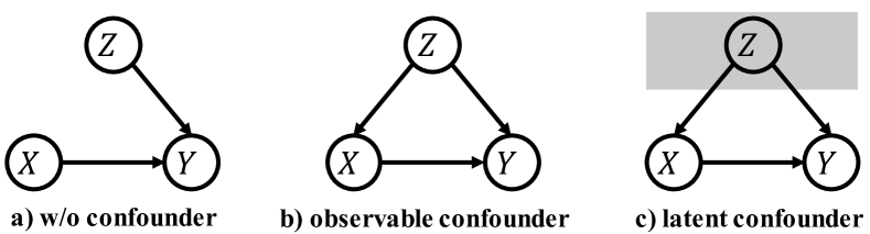
Figure 3: Three typical local structures in a causal graph.

Confounders. Despite the above challenges, existing approaches neglect one key factor—confounders—in causality analysis due to limited observability. Confounders, either observable or non-observable (called “latent confounders”), are ubiquitous and hinder causality analysis. For instance, increasing software input size $Z$ may simultaneously increase filesystem I/O $X_{1}$ and processing time $Y$. Therefore, the resulting causality model that regresses $Y$ on $X_{1}$ is biased and inaccurate. When $Z$ is observed (Fig. 3(b)), we may employ double machine learning (DML) [40] to debias. For realistic settings where $Z$ is not observed ($Z$ is a latent confounder, as in Fig. 3(c)), it is impossible to estimate an unbiased model from data [12]. The state-of-the-art (SOTA) works either assume the absence of confounders [5] (as in Fig. 3(a)) or assume that all confounders are observable [8], as in Fig. 3(b). As shown in Sec. VI-C, neglecting observable/latent confounders impedes causality analysis accuracy.

TABLE I: Comparing existing works and PerfCE. CE stands for chaos engineering. “B” and “W” in the “Scope” column denote blackbox and whitebox views, respectively.

Tool	Scope	Causal Graph	Root Cause	Counterfactual	General
		Generation	Analysis	Analysis?	KPI?
CauseInfer [6]	B	Learning with data	Graph Traversal	✗	✗
DBSherlock [41]	B	N/A	Actual Cause [42]	✗	✓
MicroScope [7]	B	Learning with data	Graph Traversal	✗	✗
Sieve [43]	B	Granger causality test	Graph Comparison	✗	✗
ExplainIt [8]	B	Learning with data	Linear Regression	✗	✓
FluxInfer [44]	B	N/A	PageRank [45]	✗	✓
iSQUAD [4]	B	N/A	BCM [46]	✗	✓
Sage [5]	B	Hand-coded rule	CVAE [47]	✓	✗
Groot [9]	W	Hand-coded rule	PageRank [45]	✗	✗
PerfCE	B	CE-enhanced learning	DML + CE-enabled IV	✓	✓

Existing Works. Table I compares PerfCE with existing works conceptually and technically. We categorize each work in terms of either rule-based or learning-based causality analysis. As aforementioned, rule-based methods are often limited to specific domains and metrics; Sage and Groot manually defined several rules to constitute causal graphs. As shown in the last column of Table I, they only support limited KPIs (e.g., network latency-related KPIs) specified in the manual rules. Sieve uses Granger causality tests to discover causal relations between the time series. It evaluates if one time series can forecast another, which is not necessarily the true causality. Most learning-based methods train causal graphs using offline data collected during normal execution; such passively collected observations (e.g., system logs) are often biased.

Moreover, given a causal graph, most works rate the contribution of identified causes using heuristics pertaining to graphical structures, e.g., PageRank-based solutions add heuristically-designed “weights” to graph edges. Such heuristics-based methods can hardly provide meaningful quantitative relations between the root cause and performance anomalies. This prevents developers from comprehending how the root cause leads to an anomaly. Methods based on graph traversal begin with abnormal KPI nodes and backtrack via their ancestors to identify the root cause. Sage applies predictive models to quantify the influence of a possible cause. Sage is the only attempt at quantitative counterfactual analysis. Sage, however, only supports quantitative analysis of network latency-related KPIs, as it primarily focuses on cloud microservices. Due to limited observability, Sage may be biased with regard to the prevalence of confounders. DBSherlock uses an actual causality framework [48, 49] to explain performance anomalies. However, it employs a simplified actual causality framework that does not explicitly distinguish cause and effect. As acknowledged in their paper, the explanation provided by them is different from the actual cause from a causality perspective.

PerfCE. CE is used for stress testing software systems and in-house (differential) testing. This paper presents CE as an almost “out-of-the-box” option for enhancing causality analysis. CE negatively affects software performance, with its chaos variables influencing numerous KPIs, providing abundant training data for learning-based causality analysis. PerfCE supports general KPIs, not limited to domain-specific instances. Instead of passively collecting system logs, PerfCE actively mutates chaos variables (influencing hundreds of KPIs) for comprehensive observability and accurate SEM learning. This active mutation is referred to as active manipulation in the paper. Additionally, PerfCE offers quantitative counterfactual analysis with (latent) confounders and arbitrary KPIs. PerfCE uses double machine learning (DML) to address observable confounders and instrumental variable (IV) to overcome latent confounders. This research uses the domain-general CE framework but doesn’t require domain-specific “steady states.” CE is not limited to assisting in-house testing, and combined with causality analysis, it can significantly improve performance debugging of (distributed) databases.

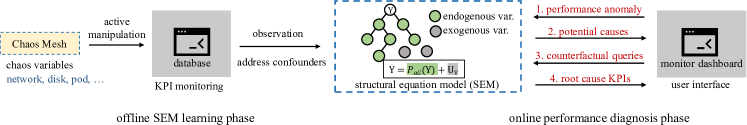
Figure 4: PerfCE overview.

IV Design of PerfCE

Fig. 4 illustrates PerfCE’s workflow, consisting of offline learning and online diagnostic phases. The learning steps (structure learning and parameter learning) are executed before deploying the database to the production environment, while the online diagnostic phase takes place after its public release, leading to the classification of these stages as offline and online, respectively. In the offline phase, PerfCE employs Chaos Mesh [13], an industry-standard CE framework integrated into cloud container environments, to launch CE toward the target databases and gather training data for constructing SEMs (Sec. IV-A). With active manipulation, CE produces high-quality SEMs, allowing PerfCE to consider both observable and latent confounders, as shown in Fig. 3. Using the learned SEM and a performance anomaly observed during online database execution, PerfCE  identifies root cause KPIs. Additionally, PerfCE enables users to pose counterfactual queries targeting the quantitatively localized root causes, such as “if CPU usage is reduced to 45%, how would the performance change?” More details can be found in Sec. IV-B.

User Querying Abnormal KPIs. We clarify that, during the online diagnosis phase, PerfCE does not need to decide if its input, a KPI, is “normal” or “abnormal.” Users can query whatever KPIs they are curious about and PerfCE will rely on the underlying causal graphs/SEMs to identify root causes that influence the queried KPIs. Nevertheless, we presume that users would query PerfCE with abnormal KPIs under performance anomaly cases; this is obviously the standard usage scenarios of PerfCE, and it is easy to see that querying a normal, uninteresting KPI is generally meaningless in our performance diagnosis context.

Application Scope. PerfCE debugs real-world database performance anomalies. Modern databases are complex and susceptible to performance issues. In our evaluation, we assess PerfCE using synthetic test suites and real-world databases (MySQL and TiDB), which are also utilized by existing works like CauseInfer [6], FluxInfer [44], and ExplainIt [8] (see details in Sec. VI-A). We deploy MySQL and TiDB in K8s clusters, the de facto system for managing containerized applications on multiple hosts. Other databases can also be integrated into K8s and analyzed by PerfCE.

IV-A Offline CE-Enhanced SEM Learning Phase

CE Usage. It is a long-standing problem in causal inference to learn high-quality SEMs from observational data. The validity of output SEMs depends on a set of assumptions. In performance diagnosis, these assumptions are frequently violated, posing obstacles to subsequent causality analysis. We employ CE in SEM learning: In (I) and (II), we explain how CE enables accurate and comprehensive SEM learning. In (III), we detail the operations for generating training data using CE.

(I) Improving Observability on Normal Data. According to the literature [10], faithfulness guarantees d-separation on causal graphs. This assumption allows for refuting causal relations without correlations. However, insufficient data can lead to a lack of correlations on causally related data. Many KPIs remain unchanged or change little in daily states, making it difficult to collect sufficient observations to the underlying system and establish causal relations. PerfCE uses Chaos Mesh for “active manipulation” during causal learning: Chaos Mesh enables mutating chaos variables to improve observability on value ranges and KPI causality. For example, mutating the “network loss probability” affects network-related KPIs, like “network duration of request.” CE explores a larger KPI value space and effectively uncovers infrequently occurring KPI states, thereby building a more accurate causal graph.

(II) Improving Observability on Anomalies. CE allows for triggering anomalies offline by heavily mutating certain chaos variables. By inspecting real performance anomalies, we find that many basic performance anomalies (e.g., “I/O Saturation”) are outcomes of the I/O-concerned chaos variable. Moreover, some complex performance anomalies (e.g., “Workload Spike”) can be simulated by combining chaos variables. This way, we not only augment the comprehensiveness of observed normal data (as in (I)), but also largely enrich the knowledge of anomaly data. This would effectively alleviate the OOD (out-of-distribution) challenge faced by previous works, which are presented in Table I, since online anomaly data was rarely seen in offline training data collected by previous research.

(III) Collecting Training Data. To collect offline training data, in addition to the constant queries emitted by workload simulators (such as the TPC-C benchmark [50]), we also use a set of chaos variables to stress the target databases. Among the chaos variables included in our experiments (see details in Sec. V), some, when enabled, directly inject faults into the target databases. When generating training data, we enable each of them and record how KPIs change. Other chaos variables are configurable, allowing us to mutate their values to determine the extent of their impact on databases. When generating training data, for each of them, we divide its valid input range equally into three to five thresholds (depending on the sensitivity of this chaos variable; more sensitive variables are mutated five times and vice versa). We mutate each chaos variable using all of its thresholds, and we collect the KPI changes for each iteration. KPIs are initially used to learn the structure of the causal graph, and then chaos variables and KPIs are used together to learn the SEM’s parameters (see details in the following paragraphs).

Causal Graph Structure Learning. Once the offline training data is gathered, we first learn causal graphs. Causal graph structure learning generates a DAG, where each node denotes one KPI and each edge represents the causal relations of a KPI pair. This enables qualitative causality analysis, such that given a performance anomaly monitored during the online phase (denoting a node on the DAG), we collect its ancestors to form the potential root causes (see details in Sec. IV-B). Previous work like CauseInfer [6] has relied heavily on constraint-based algorithms (e.g., the PC algorithm [10]), which returns an incomplete causal graph with undirected edges (CPDAG) and arbitrarily assigns directions to undirected edges. In PerfCE, we aim to harness the power of score-based algorithms to learn a causal graph that maximizes a predefined score over the observational data, with all edges in the resulting graph being directed. In particular, we employ a two-stage technique based on BLIP [51] to learn causal graphs. To begin with, for each variable, we identify its possible parent sets with local scores. We then use a global structure optimization algorithm to identify the causal graph that maximizes the global score, which is computed using cached local scores in the first stage. According to the literature [52], BLIP produces empirically much better results than the PC algorithm [10] employed in previous works. Nevertheless, PerfCE is not bounded by BLIP; we use it as it is one recent work that offers off-the-shelf implementation with good engineering quality. Users can replace BLIP with other algorithms whenever needed [10, 52].

Causal Graph Parameter Learning. Given that the DAG representing causal graph structures, we further conduct parameter learning to assign relationships toward each edge of the DAG. This step enables quantitative counterfactual analysis. Considering the sample case in Fig. 1, given filesystem I/O $X_{1}=x_{1}$ and CPU usage $X_{2}=x_{2}$, quantitative causality analysis infers the consequent processing time $Y$. For this simple case, we can directly train a predictive model that predicts $Y$ given $X_{1}$ and $X_{2}$. This trained model can be directly used to conduct counterfactual analysis, i.e., computing the ATE (refer to Eqn. 1) of $X_{1}$ or $X_{2}$ on $Y$.

However, such methods are not suitable when $X_{1}$ and $X_{2}$ have a causal relationship ($X_{1}$ forms a confounder). For instance, heavy filesystem I/O itself may result in poor CPU usage, as processes may be blocked while waiting for I/O. In this case, $X_{1}$ is an observable confounder of $X_{2}$. We start to analyze a potential solution by assuming linear causal relations and will extend it to general cases later. In this setting, $X_{1}$ is an exogenous variable, while $X_{2}$ and $Y$ are endogenous variables (Fig. 5(a)). Suppose $X_{2}=2X_{1}+b_{1}$ and $Y=X_{1}+2X_{2}+b_{2}$, where $b_{1}$ and $b_{2}$ are constants, and the zero-mean noise (or disturbance) are omitted for simplicity. As a standard solution, it is feasible to use a linear model to fit the data. However, the parameters of the learned model may be biased, which undermines subsequent counterfactual analysis (i.e., computing ATE). For instance, $Y=5X_{1}+2b_{1}+b2$ also forms a valid solution, when predicting $Y$ given $X_{1}$ and $X_{2}$. However, it fails to enable counterfactual analysis, as $X_{2}$’s effect on $Y$ is not captured. It is worth noting that this issue could impose notable challenges to any machine learning models, as long as they directly use $X_{1},X_{2}$ to regress $Y$. We now introduce how PerfCE handles observable and latent confounders.

Observable Confounders. We use double machine learning (DML) [40] to handle observable confounders. Continuing the previous example (Fig. 5(a)), DML predicts $\hat{Y}$ from $X_{1}$ and $\hat{X_{2}}$, respectively. It then estimates the relationship between the residuals by training a model to predict $Y-\hat{Y}$ using $X_{2}-\hat{X_{2}}$ as input. Finally, this model estimates the true causal effect of $X_{2}$ on $Y$ (i.e., ATE) and can be extended to arbitrary functions, including deep learning models for non-linear causal relations.

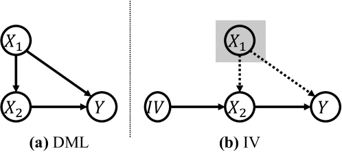
Figure 5: Counterfactual prediction using DML or IV.

Latent Confounders. The above technique is still based on the premise that all confounders (i.e., $X_{1}$ in our example) are observable. It cannot be extended to a more complex setting with latent confounders, which pervasively exist in real-world settings. Overall, the presence of latent confounders makes counterfactual predictions technically challenging, if not impossible. This is because we cannot disentangle the effect of $X_{1}$ from the causal relationship between $X_{2}$ and $Y$. We note that none of the existing works reviewed in Table I ever consider latent confounders, or they simply assume the absence of latent confounders.

A commonly-used tactic, namely instrumental variable (IV), addresses learning a regression function under an “interventional distribution” [53]. In Fig. 5(b), IV serves as the cause of treatment ($X_{2}$), and its effect on the outcome ($Y$) is propagated with $X_{2}$. A valid IV should have only one causal effect on $Y$ mediated by $X_{2}$, meaning the causal relationship between $IV$ and $Y$ must be indirect.

It is unclear how prior works can leverage IV, given that they primarily collect system logs in a passive manner. In contrast, PerfCE  novelly uses CE to form the IV, which has a direct influence on the CPU usage $X_{2}$ and an indirect effect on processing time $Y$ via $X_{2}$. We clarify that CE is proper to form IV: CE typically mutates low-level chaos variables (e.g., CPU workload, network delay time) by injecting failures. Thus, it is reasonable to assume the causal relationships between CE (through the mutated chaos variables) and the influenced “high-level” KPIs are indirect. This characteristic makes these chaos variables comply with the above prerequisite, providing a distinct opportunity to smoothly treat chaos variables as instrumental variables and apply an IV framework accordingly. Without loss of generality, we use Fig. 5(b) to illustrate the standard procedure of IV. IV first fits a model to predict $X_{2}$ from $IV$ in order to get the predicted $\hat{X_{2}}$. Then, it fits another model to predict $Y$ from $IV$ in order to get the predicted $\hat{Y}$. Afterwards, IV fits a model to predict $\hat{Y}$ from $\hat{X_{2}}$. This trained model can be used to estimate the true causal effect of $X_{2}$ on $Y$ (i.e., ATE). Similarly, this pipeline is extensible to arbitrary functions. To ensure generalizability, PerfCE uses DeepIV [12], a popular IV framework that allows counterfactual analysis with deep learning models. This helps approximate nonlinear function forms.

Input: Observed KPIs $\bm{x}=(\bm{x}_{1},\cdots,\bm{x}_{n})$, KPI of Interest $Y$, SEM $M$

Output: Ordered Potential Root Causes $\bm{X}=\{X_{i},\cdots\}$

1 $y\leftarrow\bm{x}_{Y}$; // observed KPI of interest

2 $\bm{X}_{C}=\{X_{a}\mid X_{a}\text{~{}is an ancestor of }Y\text{~{}on }M\}$; //initialize candidates

3 foreach $X_{a}\in\bm{X}_{C}$ do

4       $\hat{y}\leftarrow\mathbb{E}[Y\mid\overbrace{X_{j}=\bm{x}_{j}}^{\forall j\neq a},do(X_{a}=\mathbb{E}\left[X_{a}\right])]$;

5       $s_{a}\leftarrow\texttt{PDF}_{Y}(\hat{y})-\texttt{PDF}_{Y}(y)$;

6       assign $s_{a}$ as $X_{a}$’s blame;

7      

8 end foreach

9$\bm{X}\leftarrow\{X_{a}\mid X_{a}\in\bm{X}_{C},s_{c}>0\}$;

10 rank $\bm{X}$ by blames;

return $X$

Algorithm 1 Root Cause Analysis (RCA)

IV-B Online Root Cause Analysis

Workflow. Alg. 1 shows the root cause analysis process for performance anomalies during the online phase. $\bm{x}$ is a vector of KPIs monitored by the database, $Y$ represents the user-specified KPI of interest (e.g., query processing time), and $M$ is the SEM from the offline phase.

Assuming $Y$ is the performance anomaly KPI, indicating high database load, Alg. 1 extracts the current $Y=y$ observation from $\bm{x}$ (line 1). Next, it traverses the causal graph $M$ to find $Y$’s ancestors as potential root causes (line 2). For each candidate, the algorithm calculates its blame (lines 3–7) by predicting a counterfactual expectation under an intervention on the current $X_{a}$ (line 4). It estimates “how $Y$ would be if $X_{a}$ were normal,” where “normal” means $X_{a}=\mathbb{E}\left[X_{a}\right]$ (line 4). The blame score of $X_{a}$ is computed by comparing the probability density of $y$ and the estimated counterfactual value $\hat{y}$ (lines 5–6), where $\texttt{PDF}_{Y}$ is the probability density function of $Y$. By ranking causes by blame, Alg. 1 directs users’ attention to the most influential root cause KPIs. The following sections detail counterfactual predictions and probability densities.

Input: Observed KPIs $\bm{x}=(\bm{x}_{1},\cdots,\bm{x}_{n})$, KPI of Interest $Y$, Candidate Cause $X_{a}$, SEM $M$

Output: Counterfactual Prediction $\hat{y}$

1 $\hat{\bm{x}}\leftarrow\bm{x}$;

2 $\hat{\bm{x}_{a}}\leftarrow\mathbb{E}[X_{a}]$;

3 $\bm{X}_{D}=\{X_{d}\mid X_{d}\text{~{}is a descendant of }X_{a}\text{~{}on }M\}$;

4 sort $\bm{X}_{D}$ in the topological order on $M$;

5 foreach $X_{d}\in\bm{X}_{D}$ do

6       Total_TE $\leftarrow\sum_{X_{p}\in Pa(X_{d})}\left(\mathbb{E}[X_{d}\mid do(X_{p}=\hat{\bm{x}_{p}})]-\mathbb{E}[X_{d}\mid do(X_{p}=\bm{x}_{p})]\right)$;

7       $\hat{\bm{x}_{d}}\leftarrow\bm{x}_{d}+$Total_TE;

8       if $X_{d}$ is $Y$ then break;

9      

10 end foreach

return $\hat{\bm{x}_{Y}}$

Algorithm 2 Counterfactual Prediction

Counterfacutal Prediction. Performing counterfactual predictions is difficult, given the complexity of causal structures. As noted on line 4 of Alg. 1, we proceed with the counterfactual predictions as follows:

$$\footnotesize\hat{y}=\mathbb{E}[Y\mid\overbrace{X_{j}=\bm{x}_{j}}^{\forall j\neq a},do(X_{a}=\mathbb{E}\left[X_{a}\right])]$$ (2)

which estimates the conditional expectation of $Y$ given the currently observed KPIs $\bm{x}$ and an intervention on one KPI, $X_{a}$ while keeping the remaining KPIs ($j\neq a$) unchanged. When $X_{a}$ is a simple direct cause of $Y$, estimating Eqn. 2 is straightforward: we can simply add the average treatment effect (ATE; see Eqn. 1) of $X_{a}$ on $Y$ to the currently observed $y$. Formally,

$$\footnotesize\hat{y}=y+(\mathbb{E}[Y\mid do(X_{a}=\mathbb{E}[X_{a}])]-\mathbb{E}[Y\mid do(X_{a}=\bm{x}_{a})])$$ (3)

where the second operand (in the parentheses) of the addition represents the ATE of $X_{a}$ on $Y$, which can be further computed using the SEM learned in the offline phase.

However, in general cases where $X_{a}$ is an ancestor of $Y$, counterfactual changes on $X_{a}$ may influence other KPIs, whose changes may propagate to $Y$ as well. To systematically model the effect of $X_{a}$ on $Y$, we recursively update all $X_{a}$’s descendants on the causal graph with respect to the counterfactual change and estimate $\hat{y}$. Alg. 2 outlines the procedure. We use $\hat{\bm{x}}$ to maintain the counterfactual values of KPIs (line 1) and update $\hat{\bm{x}_{a}}$ to its mean value (line 2). With $do(X_{a}=\mathbb{E}[X_{a}])$, only the descendants of $X_{a}$ will be modified. Therefore, we estimate each of its descendants in topological order (lines 3–9) such that a descendant is updated when only all its ancestors have been updated to the counterfactual values. For each descendant $X_{d}$, we compute the total treatment effect (Total_TE) as the sum of its parents’ treatment effects on $X_{d}$ (line 6) and derive the counterfactual $X_{d}$ accordingly (line 7). When $Y$ is updated, we terminate the procedure and return $\hat{\bm{x}_{Y}}$ as the counterfactual prediction of $Y$ given the intervention of $do(X_{a}=\mathbb{E}[X_{a}])$.

Probabilistic Modeling. Computing $\texttt{PDF}_{Y}(y)$ is challenging due to the unknown distribution of $X_{k}$. Assuming a prior distribution family and estimating parameters from observations makes computing $\texttt{PDF}_{Y}(y)$ feasible. However, neither Gaussian nor beta distributions accurately estimate real-world KPIs. For instance, when dealing with multiple modals, these assumptions fall short. We use Gaussian KDE [54, 55] for non-parametric approximation, consistently yielding good performance across KPIs.

V Implementation

We implement PerfCE in 2K lines of Python code and Chaos Mesh (ver. 2.1.3) with 3K lines of yaml configuration. PerfCE works with K8s, making it compatible with various DBMSs (e.g., MySQL, PostgreSQL, TiDB) and adaptable for performance debugging in different scenarios. We use K8s due to its integration with Chaos Mesh and it enables analyzing distributed cloud databases. See the chaos variables list at [56].

Databases. We apply PerfCE to MySQL and TiDB. We follow prior works [41] and deploy MySQL with a single instance on K8s. For TiDB, we use a recommended test cluster with one PD pod, one TiDB pod, and three TiKV pods on a 3-node K8s cluster [57]. PD, TiDB, and TiKV serve as manager, interface, and storage components, respectively. In K8s, a “pod” is an application’s minimal unit. The 3-node cluster consists of a control-plane and two worker nodes.

KPI Monitoring. PerfCE uses Grafana [58] and Prometheus [59] for KPI monitoring in K8s. The details of our employed KPIs can be found in [60, 61]. PerfCE records each KPI’s value every one second.

Offline Training. Sec. IV-A explains that PerfCE extends the codebase of BLIP [51] to learn causal graphs. We adopt BLIP due to its SOTA performance and high engineering quality. We extend its codebase with 112 extra lines of Python code. PerfCE is orthogonal to particular causal graph learning algorithms. We leave it as one future work to explore leveraging other SOTA algorithms like REAL [52] and ML4C [62]. We employ EconML [63] to perform double machine learning and DeepIV [12] to estimate the parameters of causal relationships, where random forest models and neural networks (Multi Layer Perception) are jointly employed for regression. We present model details in the Supplementary Material [16].

VI Evaluation

We conduct extensive evaluations on MySQL in Sec. VI-A to demonstrate PerfCE’s effectiveness in practice. To study its scalability, we evaluate PerfCE on a large distributed DBMS, TiDB, in Sec. VI-B. In addition, we compare PerfCE’s counterfactual analysis with machine learning models on synthetic data in Sec. VI-C.

Processing Time. For data collection, we run the database for six hours without chaos mesh experiments. Then, we execute a 12-hour chaos mesh workflow on MySQL and a 20-hour workflow on TiDB. Each workflow comprises multiple chaos experiments, with a 10-minute suspend period between them. Thus, we gather 18 hours of MySQL data and 26 hours of TiDB data. While chaos mesh introduces non-trivial overhead, prior works [41, 44, 5] often collect data over longer periods.

The offline training phase is a one-shot effort. Users should be more concerned with potential online overhead: PerfCE incurs negligible online overhead, as all online analysis tasks are rapid. For MySQL, it takes about 50 minutes for causal graph structure offline learning and 8 minutes for parameter learning. Analyzing one performance anomaly (quantitative and qualitative aspects) takes less than a minute. For TiDB, PerfCE requires about 1.3 hours for causal graph learning and 40 minutes for parameter learning. In the online inference phase, each anomaly analysis takes 3 to 5 minutes, depending on the number of involved KPIs. Evaluating synthetic datasets takes several seconds.

VI-A Evaluation on Effectiveness

TABLE II: Performance anomalies on MySQL.

Component	Anomaly	Component	Anomaly
Client	Workload Spike	I/O	I/O Saturation
Database	Database Backup		I/O Latency
	Database Restore		I/O Fault
	Flush Log	Network	Network Delay
	Flush Table		Network Partition
Memory	Memory Stress	CPU	CPU Stress

Environment and Data Collection. We set up a MySQL instance on K8s, and execute TPC-C queries using BenchBase [64] for a duration of 18 hours. To collect relevant KPIs, we utilize mysql-exporter [65], covering a total of 79 KPIs. During the online phase, we simulate performance anomalies by following the configuration in DBSherlock [41], as shown in Table II. These anomalies correspond to various key components in MySQL. In total, we create 13 anomaly instances that could potentially have negative effects on user-focused KPIs (e.g., Query_Duration).

Baselines. We re-implement CauseInfer [6], FluxInfer [44], and ExplainIt [8] as baseline methods, as reviewed in Table I. For CauseInfer [6], we implement a variant (CauseInfer+CE) by augmenting its causal discovery process with our CE module. We exclude methods without general KPI support and omit DBSherlock [41] and iSQUAD [4], as they require labeling normal and abnormal regions during the offline phase.

Human Evaluation Setup. PerfCE and three baseline methods provide ranked KPI lists, and we collect the top-5 KPIs for each anomaly experiment. We invite ten experts to select relevant KPIs from those recommended by at least one method. After briefing them on the database performance debugging scenario and KPI meanings, they choose KPIs closely related to each anomaly’s root cause. Each KPI is assigned a score as $\frac{\text{\# vote}}{\text{\# participant}}$ for a given anomaly, with a higher score indicating a higher expert consensus. Treating expert-selected KPIs as ground truth, we evaluate the methods’ effectiveness in identifying root causes. The average completion time is 45 minutes, with details in the supplementary material.

Metric. Using the scores from human evaluation, we consider the following metrics for comparison. We compute the average score (AS) of the top-1/3/5 KPIs suggested by each method. Additionally, we employ MAP@R (Mean Average Precision) and NDCG (Normalized Discounted Cumulative Gain), two widely-used metrics in recommendation systems, to evaluate the accuracy of the ranked KPI lists in relation to user preferences.

TABLE III: Comparison of different methods. #Anomaly denotes the number of anomalies in this component. We highlight the best and second best methods in each component.

Component	Metric	PerfCE	CauseInfer	CauseInfer+CE	FluxInfer	ExplainIt
(#Anomaly)
Client (1)	Top-1 AS	0.70	0.00	0.00	0.90	0.00
	Top-3 AS	0.73	0.00	0.00	0.90	0.20
	Top-5 AS	0.80	0.00	0.00	0.70	0.12
	MAP@R	0.36	0.00	0.00	0.41	0.02
	NDCG	0.82	0.00	0.00	0.81	0.11
Database (4)	Top-1 AS	0.40	0.00	0.18	0.40	0.00
	Top-3 AS	0.49	0.14	0.32	0.36	0.05
	Top-5 AS	0.56	0.09	0.28	0.40	0.09
	MAP@R	0.17	0.02	0.10	0.13	0.01
	NDCG	0.65	0.11	0.38	0.45	0.08
I/O (4)	Top-1 AS	0.93	0.40	0.25	0.23	0.03
	Top-3 AS	0.81	0.28	0.43	0.15	0.08
	Top-5 AS	0.76	0.18	0.37	0.25	0.18
	MAP@R	0.30	0.08	0.12	0.08	0.03
	NDCG	0.91	0.27	0.42	0.28	0.16
Network (2)	Top-1 AS	0.90	0.35	0.20	0.20	0.00
	Top-3 AS	0.90	0.25	0.37	0.12	0.08
	Top-5 AS	0.90	0.15	0.32	0.24	0.15
	MAP@R	0.34	0.07	0.10	0.08	0.03
	NDCG	0.99	0.22	0.33	0.25	0.13
Memory (1)	Top-1 AS	1.00	1.00	0.70	0.70	0.00
	Top-3 AS	1.00	0.33	0.80	0.23	0.00
	Top-5 AS	1.00	0.33	0.70	0.36	0.20
	MAP@R	0.17	0.08	0.63	0.25	0.03
	NDCG	1.00	0.32	0.92	0.51	0.17
CPU (1)	Top-1 AS	0.60	0.00	0.00	0.30	0.00
	Top-3 AS	0.60	0.00	0.00	0.77	0.00
	Top-5 AS	0.60	0.00	0.00	0.66	0.12
	MAP@R	0.12	0.00	0.00	0.51	0.02
	NDCG	0.60	0.00	0.00	0.74	0.09
Overall (13)	Top-1 AS	0.72	0.25	0.22	0.37	0.01
	Top-3 AS	0.72	0.19	0.35	0.32	0.07
	Top-5 AS	0.73	0.13	0.30	0.37	0.14
	MAP@R	0.25	0.05	0.12	0.17	0.02
	NDCG	0.80	0.18	0.37	0.42	0.12

Result Overview. We report the results of Top-1/3/5 Average Score (AS), MAP@R and NDCG in Table III. We observe that PerfCE  substantially outperforms existing methods for nearly all settings. For instance, its overall NDCG is 90.5% higher than the second best method, FluxInfer. It also provides the best root causes for five out of seven anomaly components compared to the baseline methods. In short, we consider PerfCE to be sufficient enough to produce reasonable KPIs to assist developers in identifying the root cause. Empirical results also show that CE offers a general augmentation toward causality-based approaches. As shown in Table III, after being augmented with CE, CauseInfer manifests much better performance in most settings (106% and 120% improvement on the overall NDCG and MAP@R scores, respectively) and provides better root causes compared to its original version. We also observe that the gaps between PerfCE and other methods like CauseInfer+CE vary across different settings. For example, in the Network component, PerfCE outperforms CauseInfer+CE by 66% in NDCG. Here, CauseInfer+CE only identifies five causes out of 14, while PerfCE correctly identifies most of the root causes, which yield the large gap in the Network component. In contrast, in the Database component, the difference is only 20%. We find that, out of four cases in the Database component, PerfCE provides the best results in three cases while being sub-optimal in the “Flush Log”.

Error Analysis. PerfCE has sub-optimal results in a few settings. We find that PerfCE recommends one KPI for the anomaly triggered by memory stress (5th component in Table III) and CPU stress (6th component). Therefore, AS is computed using the only KPI. For memory stress, PerfCE recommends “Node.Memory_Distribution_Free”, which is voted by all human experts and thus assigned a score of 1. Thus, its Top-1/3/5 AS and NDCG are computed as 1.00. However, experts also annotate some other useful albeit less important KPIs with lower scores (e.g., “MySQL.Query_Cache_Mem_Free_Mem”). Thus, when a method (e.g., CauseInfer) recommends more KPIs besides “Node.Swap_Activity_Swap_In”, it gains a higher MAP score. We inspect the cause of this inaccuracy and find that it is primarily due to inaccurate counterfactual analysis over a lengthy causal chain (with 11 hops on causal graphs), where regression errors are accumulated and propagated, resulting in inaccurate estimations.

In another case where an anomaly was triggered by CPU stress (6th component in Table III), PerfCE also fails to suggest several highly relevant KPIs. We find that it is due to the inaccurate causal graph, where the causal relations between the KPI of interest (i.e., “Query_Duration”) and many CPU-related KPIs are incorrectly missed. Performance of baseline methods downgrades as well. Given the inherent difficulty of causal structure learning, we anticipate that PerfCE users will incorporate domain knowledge to revise certain spurious edges and improve the quality of causal graphs. In particular, according to domain knowledge and experts’ feedback, we notice that CPU usage is causally related to memory and IO activities. Hence, we manually add four edges from “Node.CPU_Usage_Load_user” and “Node.CPU_Usage-_Load_1m” pointing to “Node.Memory_Distribution_Free” and “Node.Memory_IO_Activity”. After this, PerfCE’s performance is improved from 0.12 to 0.30 on the MAP@R score and from 0.60 to 0.67 on the NDCG score, respectively.

TABLE IV: Statistics of generated causal graphs. #Node and #Edge denotes the number of non-isolated nodes/edges in the causal graphs. BIC denotes Bayesian Information Criterion.

Method	#Node	#Edge	BIC	Accuracy
PerfCE w/o CE	64	63	-614055.5	0.73
PerfCE	78	89	-584910.3	0.87
Improvement	+22%	+42%	+6%	+16%

Causal Graph Accuracy. We report the statistics of causal graphs generated by PerfCE and its ablated version (PerfCE w/o CE) that excludes the CE module in Table IV. BIC score is a standard metric for assessing the “fitness” of causal graphs on observational data. Accuracy is a metric examining whether the pairwise correlations are properly represented in the causal graph in terms of d-separations and d-connections. We refer readers to [66] for the full details of these metrics. The two metrics are computed using the unseen data collected during the online phase. For both metrics, a greater value indicates a better fitness with online data. We interpret the overall results as encouraging: 78 out of 79 KPIs (after excluding constantly unchanged KPIs) are not isolated in the causal graph, and 26 additional edges are identified compared to the ablated version. Furthermore, PerfCE manifests a high degree of agreement with the unseen online data, with an accuracy of 0.87. The improvements in the BIC score further demonstrate the effectiveness of CE. We supply the full graph in Supplementary Material [16]. Overall, we consider that the PerfCE’s causal discovery can learn an accurate causal graph, and CE facilitates learning the causal graph with much better quality.

VI-B Evaluation on Scalability

Environment. We also evaluate PerfCE on a distributed database, TiDB. As in Sec. V, we host TiDB on a K8s cluster with three TiKV pods (tikv-0,1,2), one TiDB pod (tidb), and one PD pod (pd). As noted in Sec. V, 254 KPIs are involved in the TiDB scenario, which is much larger than MySQL. Thus, we view this evaluation as appropriate to benchmark the scalability of PerfCE on real-world distributed databases. We present two case studies by imposing two anomalies to TiDB: tidb-pod-failure and network-loss. tidb-pod-failure injects a failure directly into the TiDB pod and makes it temporally unavailable. tikv-0-network-loss randomly drops 80% packets that are sent to a specific KV pod (i.e., tikv-0). Since the way to trigger performance anomalies (i.e., the ground truth) is known in our experiments, we employ domain knowledge to justify whether PerfCE’s outputs are consistent with the ground truth.

TABLE V: Top-10 KPIs suggested by PerfCE for answering tidb-pod-failure.

Rank	KPI Family	Description
1-5	Lock Resolve OPS	The number of TiDB operations that resolve
		locks. When a TiDB pod fails, TiDB-related
		operations would decrease.
6, 9	Statement OPS	The number of different SQL statements
		executed per second by TiDB pod. When a
		TiDB pod fails, it would be unable to
		execute statements.
7, 8	CPS By Instance (OK)	The succeed command statistics on each TiDB
		instance. When a TiDB pod fails, the number
		of succeed commands would decrease.
10	KV Cmd OPS	The number of executed KV commands emitted
		by TiDB pod. When a TiDB pod fails, it
		would be unable to execute statements.

TABLE VI: Top-10 KPIs suggested by PerfCE for answering tikv-0-network-loss.

Rank	KPI Family	Description
1, 3, 7	TiKV Write Leader	The number of leaders that are writing on each
		TiKV instance. When network packets to a TiKV
		pod are constantly lost, writes on this TiKV pod
		would decrease and writes on other pods would
		increase.
2, 4-6, 10	TiKV Resource	The usage of resources (e.g., CPU and memory)
		on each TiKV instance. When network packets
		to a TiKV pod is constantly lost, it would process
		less requests thus uses less resources, while
		others are responsible for more requests and
		use more resources.
8, 9	Duration	The duration for processing different activities.
		When network packets to a TiKV pod is constantly
		lost, the duration of completing different
		activities would increase.

Case 1: In tidb-pod-failure, we inject a failure to the TiDB pod. Then, we observe that the duration of the request launched by PD pod (i.e., “Handle Requests Duration”) becomes abnormal and ask PerfCE to diagnose this anomaly. In short, we group the top-10 KPIs suggested by PerfCE and use TiDB’s official documentation to comprehend each of them. As shown in Table V, while the target KPI (PD’s request duration) is not directly relevant to TiDB pod failure, we find that all top-10 KPIs suggested by PerfCE are highly relevant to the root cause. All of the KPIs indicate the exact different activities performed by the failed TiDB pod. Therefore, we interpret the outputs of PerfCE as reasonable and highly informative: when users are provided with these KPIs, it should be accurate to assume that they can easily identify the anomaly’s root cause.

Case 2: In tikv-0-network-loss, a notable proportion of network packets are dropped, reducing the overall performance of the database. In particular, we observe that the duration of command completion, “Completed Commands Duration (seconds)”, is abnormal, and we apply PerfCE  for root cause analysis. We group and present the results of PerfCE in Table VI. We find the outputs of PerfCE to be valuable. Note that the affected TiKV pod (tikv-0) can only serve limited functionality, while other pods (tikv-1,2) would serve extra responsibilities. Therefore, the decrease in workload on tikv-0 and the surge in workload on tikv-1,2 are reasonable and should provide enough hints for users to investigate the detailed status of tikv-0.

VI-C Evaluation on Counterfactual Analysis

This section evaluates if PerfCE provides satisfactory counterfactual analysis results under complex causal graphs. Collecting ground-truth outcomes of quantitative counterfactual changes in real-world DBMSs is challenging, if not impossible (hence the human evaluation in Sec. VI-A). Therefore, we use synthetic data, a common setup for evaluating causal inference algorithms, to compare PerfCE and other baselines.

TABLE VII: DGP models for generating synthetic data. LS stands for local structure.

LS (see Fig. 3)	Formulation
(a) no confounder	$X_{1}\sim\text{Uniform}(-1,1)$
	$X_{2}\sim\text{Uniform}(-1,1)$
	$Y=\theta_{1}(X_{1})+\theta_{2}(X_{2})+\epsilon,\epsilon\sim\text{Uniform}(-1,1)$
(b) observable confounder	$X_{1}\sim\text{Uniform}(-1,1)$
	$X_{2}=\theta_{1}(X_{1})+\eta,\eta\sim\text{Uniform}(-1,1)$
	$Y=\theta_{2}(X_{1})+\theta_{3}(X_{2})+\epsilon,\epsilon\sim\text{Uniform}(-1,1)$
(c) latent confounder	$IV\sim\text{Uniform}(-1,1)$
	$X_{1}\sim\text{Uniform}(-1,1)$ (unobserved)
	$X_{2}=\theta_{1}(X_{1})+\theta_{2}(IV)+\eta,\eta\sim\text{Uniform}(-1,1)$
	$Y=\theta_{3}(X_{1})+\theta_{4}(X_{2})+\epsilon,\epsilon\sim\text{Uniform}(-1,1)$

DGP Model. Following common practice in causality analysis [63, 67], we formulate a set of DGP (Data Generating Process) models [63] for evaluation in Table VII. These models correspond to the local structures (with confounders) in Sec. IV-A. We use a linear form for $\theta$ and define all exogenous variables to follow a uniform distribution. Then, we generate $100$ datasets for each DGP model using different random states, resulting in 300 ($3\times 100$) DGP models. For each model, we train with 5,000 data samples and create 1,000 counterfactual queries. Each query answers the treatment effects of changing $X_{2}=x_{2}$ to $X_{2}=x_{2}^{\prime}$ when $X_{1}=x_{1}$, where $x_{1},x_{2},x_{2}^{\prime}$ are generated randomly and the ground-truth treatment effects are generated by the specification of $Y$ in DGP models.

Baseline & Metric. We use Multi Layer Perception (MLP), Random Forest (RF), Decision Tree with Pruning (DTP), and Support Vector Machine (SVM) as baseline methods, treating counterfactual analysis as a regression problem. The MLP model has three hidden layers and uses the Adam optimizer [68] with default parameters. We use default parameters for all models and report MSE (mean squared error; lower is better) and $R^{2}$ (coefficient of determination; higher is better) for each method on datasets generated by each DGP model.

TABLE VIII: MSE and $R^{2}$ on synthetic data. LS stands for local structure. Best metrics are highlighted.

LS	Metric		PerfCE	MLP	RF	DTP	SVM
(a)	MSE	mean	0.0003	0.0020	0.0109	0.0634	0.0003
		std	0.0003	0.0011	0.0020	0.0228	0.0005
	$R^{2}$	mean	0.9988	0.9914	0.9522	0.7422	0.9983
		std	0.0018	0.0063	0.0297	0.1456	0.0029
(b)	MSE	mean	0.0002	0.0030	0.0176	0.1206	0.0003
		std	0.0003	0.0022	0.0072	0.0549	0.0005
	$R^{2}$	mean	0.9988	0.9875	0.9282	0.4949	0.9983
		std	0.0019	0.0093	0.0463	0.3501	0.0028
(c)	MSE	mean	0.0174	0.3758	0.1029	0.0815	0.0389
		std	0.0302	0.2098	0.0960	0.0337	0.0289
	$R^{2}$	mean	0.9382	-0.8258	0.1540	0.5733	0.7797
		std	0.0936	1.9738	1.2979	0.3894	0.2619

Table VIII shows that PerfCE excels in almost all settings. While SVM has comparable MSE performance in LS (a), this is reasonable since PerfCE and SVM are asymptotically equivalent without confounders. However, SVM’s performance declines in LS (b) and (c). Specifically, in LS (c), the MLP model overfits the data, resulting in unsatisfactory and unstable performance. This downgrade is reasonable, as the MLP model cannot distinguish the effects of $X_{1},X_{2}$ on $Y$ from the data generated by DGP models under LS (c). Other models exhibit similar downgrades. In contrast, PerfCE accurately estimates the effects of $X_{2}$ on $Y$ across all settings, even with latent confounders, as in LS (c).

VII Discussion and Threats to Validity

Capturing Temporal Characteristics of KPIs. Like most related works [6, 7, 8], this research assumes KPI observations are independent and identically distributed (iid), making causality analysis feasible. However, KPIs may exhibit temporal characteristics in reality, potentially leading to missed edges in causal structure learning and inaccurate counterfactual analysis estimations. As causal discovery and inference on time series remain largely understudied, we defer considering the temporal properties of KPIs in counterfactual analysis to future research.

Enhancing CE. We recognize that the current usage of Chaos Mesh is suboptimal, particularly due to redundancy among CE experiments. Minimizing the number of experiments while maximizing causality analysis observability presents a challenging problem for future exploration. We expect that certain “feedback-driven” mutations (analogous to feedback-driven fuzz testing [69]) can be applied when mutating chaos variables, reducing invocations of Chaos Mesh.

Threats to Validity. One threat is that the evaluation of PerfCE is limited to two real-world databases and our conclusion may not generalize to other databases. Another relevant threat is on the potentially limited set of performance anomalies, as we mainly focus on database response time. We mitigate these threats by designing PerfCE whose technical pipeline is independent of specific databases or response time. We envision that PerfCE is applicable to other scenarios like cloud containerization systems, and PerfCE can diagnose other performance anomalies like database throughput.

VIII Related Work

Theoretical Causality Analysis. Causality analysis is the foundation of scientific discovery, with applications in the fields of economics and clinical trials [53]. Identifying qualitative (i.e., SEM structure learning) and quantitative (i.e., SEM parameter learning) causal relationships is challenging. Typically, causal discovery algorithms are applied to learn a causal graph that encodes qualitative causal relationships among a set of variables. Recent years have witnessed a surge of interest in causal discovery [51, 67, 52, 70, 71, 72, 73]. Without clear qualitative causal relationships, causal inference (i.e., identifying quantitative causal relationships) is infeasible or inaccurate. The methods for causal inference are diverse, including actual causality [42] and potential outcomes framework [74, 75] proposed by Rubin. PerfCE uses Rubin’s framework because it is more suitable when KPIs are modeled as random variables and the ATE (average treatment effect) naturally allows for propagating influence over causal paths.

Applications of Causality Analysis. Recently, there have been a number of researches that applied causality analysis to address problems in software engineering [76, 77, 78, 79, 80]. These tools usually focus on analyzing how program inputs or configurations impact the software behavior (e.g., execution time or crash). In addition, causality analysis is used extensively in the field of machine learning due to its inherent interpretability [81, 82, 83, 84, 85, 86]. We also believe that causality analysis can have a broader application in software engineering because it can systematically handle interactions among many variables; we will explore the usage of causality analysis in other fields like testing and static analysis in the future.

IX Conclusion

We have presented PerfCE for database performance anomaly diagnosis. PerfCE  novelly employs Chaos Mesh for augmenting causality-based performance debugging, and it features both qualitative root cause identification and quantitative counterfactual analysis and addresses several challenges in the process. Evaluations on synthetic and real scenarios show that PerfCE offers accurate diagnosis and outperforms existing works across nearly all settings.

References

- [1] “How slow database queries can negatively impact your business,” https://wire19.com/how-slow-database-queries-can-negatively-impact-your-business, 2019.
- [2] “Amazon found every 100ms of latency cost them 1% in sales,” https://www.gigaspaces.com/blog/amazon-found-every-100ms-of-latency-cost-them-1-in-sales, 2019.
- [3] “Marissa mayer at web 2.0,” http://glinden.blogspot.com/2006/11/marissa-mayer-at-web-20.html, 2006.
- [4] M. Ma, Z. Yin, S. Zhang, S. Wang, C. Zheng, X. Jiang, H. Hu, C. Luo, Y. Li, N. Qiu et al., “Diagnosing root causes of intermittent slow queries in cloud databases,” Proceedings of the VLDB Endowment, vol. 13, no. 8, pp. 1176–1189, 2020.
- [5] Y. Gan, M. Liang, S. Dev, D. Lo, and C. Delimitrou, “Sage: practical and scalable ml-driven performance debugging in microservices,” in Proceedings of the 26th ACM International Conference on Architectural Support for Programming Languages and Operating Systems, 2021, pp. 135–151.
- [6] P. Chen, Y. Qi, P. Zheng, and D. Hou, “Causeinfer: Automatic and distributed performance diagnosis with hierarchical causality graph in large distributed systems,” in IEEE INFOCOM 2014-IEEE Conference on Computer Communications. IEEE, 2014, pp. 1887–1895.
- [7] J. Lin, P. Chen, and Z. Zheng, “Microscope: Pinpoint performance issues with causal graphs in micro-service environments,” in International Conference on Service-Oriented Computing. Springer, 2018, pp. 3–20.
- [8] V. Jeyakumar, O. Madani, A. Parandeh, A. Kulshreshtha, W. Zeng, and N. Yadav, “Explainit!–a declarative root-cause analysis engine for time series data,” in Proceedings of the 2019 International Conference on Management of Data, 2019, pp. 333–348.
- [9] H. Wang, Z. Wu, H. Jiang, Y. Huang, J. Wang, S. Kopru, and T. Xie, “Groot: An event-graph-based approach for root cause analysis in industrial settings,” in 2021 36th IEEE/ACM International Conference on Automated Software Engineering (ASE). IEEE, 2021, pp. 419–429.
- [10] P. Spirtes, C. N. Glymour, R. Scheines, and D. Heckerman, Causation, prediction, and search. MIT press, 2000.
- [11] P. R. Rosenbaum and D. B. Rubin, “The central role of the propensity score in observational studies for causal effects,” Biometrika, vol. 70, no. 1, pp. 41–55, 1983.
- [12] J. Hartford, G. Lewis, K. Leyton-Brown, and M. Taddy, “Deep iv: A flexible approach for counterfactual prediction,” in International Conference on Machine Learning. PMLR, 2017, pp. 1414–1423.
- [13] “Chaos mesh: A powerful chaos engineering platform for kubernetes,” https://chaos-mesh.org/, 2022.
- [14] “TiDB,” https://github.com/pingcap/tidb, 2022.
- [15] “Kubernetes,” https://kubernetes.io/, 2022.
- [16] “Research artifact,” https://anonymous.4open.science/r/PerfCE-85E0, 2022.
- [17] “Anonymous documentation of perfce,” http://perfce.ignorelist.com/.
- [18] “Pod,” https://kubernetes.io/docs/concepts/workloads/pods/, 2022.
- [19] J. A. Jones and M. J. Harrold, “Empirical evaluation of the tarantula automatic fault-localization technique,” in Proceedings of the 20th IEEE/ACM international Conference on Automated software engineering, 2005, pp. 273–282.
- [20] B. Liblit, M. Naik, A. X. Zheng, A. Aiken, and M. I. Jordan, “Scalable statistical bug isolation,” in Proceedings of the 2005 ACM SIGPLAN conference on Programming language design and implementation, 2005, pp. 15–26.
- [21] C. Liu, L. Fei, X. Yan, J. Han, and S. P. Midkiff, “Statistical debugging: A hypothesis testing-based approach,” IEEE Transactions on software engineering, vol. 32, no. 10, pp. 831–848, 2006.
- [22] M. Attariyan, M. Chow, and J. Flinn, “X-ray: Automating Root-Cause diagnosis of performance anomalies in production software,” in 10th USENIX Symposium on Operating Systems Design and Implementation (OSDI 12), 2012, pp. 307–320.
- [23] X. Zhao, K. Rodrigues, Y. Luo, D. Yuan, and M. Stumm, “Non-Intrusive performance profiling for entire software stacks based on the flow reconstruction principle,” in 12th USENIX Symposium on Operating Systems Design and Implementation (OSDI 16), 2016, pp. 603–618.
- [24] C.-P. Bezemer, J. Pouwelse, and B. Gregg, “Understanding software performance regressions using differential flame graphs,” in 2015 IEEE 22nd International Conference on Software Analysis, Evolution, and Reengineering (SANER). IEEE, 2015, pp. 535–539.
- [25] E. Soremekun, L. Kirschner, M. Böhme, and A. Zeller, “Locating faults with program slicing: an empirical analysis,” Empirical Software Engineering, vol. 26, no. 3, pp. 1–45, 2021.
- [26] G. Jin, A. Thakur, B. Liblit, and S. Lu, “Instrumentation and sampling strategies for cooperative concurrency bug isolation,” in Proceedings of the ACM international conference on Object oriented programming systems languages and applications, 2010, pp. 241–255.
- [27] Z. Zuo, L. Fang, S.-C. Khoo, G. Xu, and S. Lu, “Low-overhead and fully automated statistical debugging with abstraction refinement,” in Proceedings of the 2016 ACM SIGPLAN International Conference on Object-Oriented Programming, Systems, Languages, and Applications, 2016, pp. 881–896.
- [28] B. Gregg, Systems performance: enterprise and the cloud. Pearson Education, 2014.
- [29] J. Tuya, J. Dolado, M. J. Suarez-Cabal, and C. de la Riva, “A controlled experiment on white-box database testing,” ACM SIGSOFT Software Engineering Notes, vol. 33, no. 1, pp. 1–6, 2008.
- [30] E. Costante, J. den Hartog, M. Petković, S. Etalle, and M. Pechenizkiy, “A white-box anomaly-based framework for database leakage detection,” Journal of Information Security and Applications, vol. 32, pp. 27–46, 2017.
- [31] J. Peters, D. Janzing, and B. Schölkopf, Elements of causal inference: foundations and learning algorithms. The MIT Press, 2017.
- [32] P. W. Holland, “Statistics and causal inference,” Journal of the American statistical Association, vol. 81, no. 396, pp. 945–960, 1986.
- [33] J. Pearl and T. Verma, “A theory of inferred causation,” in Proceedings of the Second International Conference on Principles of Knowledge Representation and Reasoning, 1991, pp. 441–452.
- [34] A. Balke and J. Pearl, “Probabilistic evaluation of counterfactual queries,” in Probabilistic and Causal Inference: The Works of Judea Pearl, 2022, pp. 237–254.
- [35] “Principles of chaos engineering,” https://principlesofchaos.org, 2022.
- [36] “Sqlsmith,” https://github.com/anse1/sqlsmith, 2021.
- [37] M. Rigger and Z. Su, “Testing database engines via pivoted query synthesis,” in 14th USENIX Symposium on Operating Systems Design and Implementation (OSDI 20), 2020, pp. 667–682.
- [38] K. Kallas, F. Niksic, C. Stanford, and R. Alur, “DiffStream: Differential output testing for stream processing programs,” Proceedings of the ACM on Programming Languages, vol. 4, no. OOPSLA, pp. 1–29, 2020.
- [39] T. Sotiropoulos, S. Chaliasos, V. Atlidakis, D. Mitropoulos, and D. Spinellis, “Data-oriented differential testing of object-relational mapping systems,” in 2021 IEEE/ACM 43rd International Conference on Software Engineering (ICSE). IEEE, 2021, pp. 1535–1547.
- [40] V. Chernozhukov, D. Chetverikov, M. Demirer, E. Duflo, C. Hansen, W. Newey, and J. Robins, “Double/debiased machine learning for treatment and causal parameters,” arXiv preprint arXiv:1608.00060, 2016.
- [41] D. Y. Yoon, N. Niu, and B. Mozafari, “Dbsherlock: A performance diagnostic tool for transactional databases,” in Proceedings of the 2016 International Conference on Management of Data, 2016, pp. 1599–1614.
- [42] J. Y. Halpern and J. Pearl, “Causes and explanations: A structural-model approach. part i: Causes,” The British journal for the philosophy of science, 2020.
- [43] Y. Gan, Y. Zhang, K. Hu, D. Cheng, Y. He, M. Pancholi, and C. Delimitrou, “Seer: Leveraging big data to navigate the complexity of performance debugging in cloud microservices,” in Proceedings of the twenty-fourth international conference on architectural support for programming languages and operating systems, 2019, pp. 19–33.
- [44] P. Liu, S. Zhang, Y. Sun, Y. Meng, J. Yang, and D. Pei, “Fluxinfer: Automatic diagnosis of performance anomaly for online database system,” in 2020 IEEE 39th International Performance Computing and Communications Conference (IPCCC). IEEE, 2020, pp. 1–8.
- [45] Y. Li, “Toward a qualitative search engine,” IEEE Internet Computing, vol. 2, no. 4, pp. 24–29, 1998.
- [46] B. Kim, C. Rudin, and J. A. Shah, “The bayesian case model: A generative approach for case-based reasoning and prototype classification,” Advances in neural information processing systems, vol. 27, 2014.
- [47] K. Sohn, H. Lee, and X. Yan, “Learning structured output representation using deep conditional generative models,” Advances in neural information processing systems, vol. 28, 2015.
- [48] J. Y. Halpern and J. Pearl, “Causes and explanations: A structural-model approach. part i: Causes,” The British journal for the philosophy of science, 2005.
- [49] ——, “Causes and explanations: A structural-model approach. part ii: Explanations,” The British journal for the philosophy of science, 2005.
- [50] T. P. P. Council, “Tpc-c benchmark,” https://www.tpc.org/tpcc, 2022.
- [51] M. Scanagatta, C. P. de Campos, G. Corani, and M. Zaffalon, “Learning bayesian networks with thousands of variables,” Advances in neural information processing systems, vol. 28, 2015.
- [52] R. Ding, Y. Liu, J. Tian, Z. Fu, S. Han, and D. Zhang, “Reliable and efficient anytime skeleton learning,” in Proceedings of the AAAI Conference on Artificial Intelligence, vol. 34, no. 06, 2020, pp. 10 101–10 109.
- [53] J. Pearl, Causality. Cambridge university press, 2009.
- [54] M. Rosenblatt, “Remarks on some nonparametric estimates of a density function,” The Annals of Mathematical Statistics, vol. 27, no. 3, pp. 832–837, 1956.
- [55] E. Parzen, “On estimation of a probability density function and mode,” The annals of mathematical statistics, vol. 33, no. 3, pp. 1065–1076, 1962.
- [56] “Chaos variables,” https://anonymous.4open.science/r/PerfCE-85E0/supplement/chaos_var.md.
- [57] “TiDB-config,” https://docs.pingcap.com/tidb-in-kubernetes/stable/get-started, 2022.
- [58] “Grafana,” https://grafana.com, 2021.
- [59] “Prometheus,” https://prometheus.io, 2021.
- [60] “Mysql kpis,” https://anonymous.4open.science/r/PerfCE-85E0/supplement/kpi.md.
- [61] PingCAP, “Tidb kpis,” https://docs.pingcap.com/tidb/stable/grafana-overview-dashboard, 2022.
- [62] H. Dai, R. Ding, Y. Jiang, S. Han, and D. Zhang, “Ml4c: Seeing causality through latent vicinity,” arXiv preprint arXiv:2110.00637, 2021.
- [63] “Econml: A python package for ml-based heterogeneous treatment effects estimation,” https://github.com/microsoft/EconML, 2022.
- [64] D. E. Difallah, A. Pavlo, C. Curino, and P. Cudré-Mauroux, “Oltp-bench: An extensible testbed for benchmarking relational databases,” PVLDB, vol. 7, no. 4, pp. 277–288, 2013. [Online]. Available: http://www.vldb.org/pvldb/vol7/p277-difallah.pdf
- [65] “Exporter for mysql server metrics,” https://github.com/prometheus/mysqld_exporter, 2022.
- [66] “Pgmpy,” https://pgmpy.org/metrics/metrics.html, 2022.
- [67] X. Zheng, B. Aragam, P. K. Ravikumar, and E. P. Xing, “Dags with no tears: Continuous optimization for structure learning,” Advances in Neural Information Processing Systems, vol. 31, 2018.
- [68] D. P. Kingma and J. Ba, “Adam: A method for stochastic optimization,” arXiv preprint arXiv:1412.6980, 2014.
- [69] M. Zalewski, “American Fuzzy Lop (AFL),” https://lcamtuf.coredump.cx/afl/, 2021.
- [70] P. Ma and S. Wang, “Mt-teql: evaluating and augmenting neural nlidb on real-world linguistic and schema variations,” Proceedings of the VLDB Endowment, vol. 15, no. 3, pp. 569–582, 2021.
- [71] L. Lorch, J. Rothfuss, B. Schölkopf, and A. Krause, “Dibs: Differentiable bayesian structure learning,” Advances in Neural Information Processing Systems, vol. 34, pp. 24 111–24 123, 2021.
- [72] P. Ma, R. Ding, H. Dai, Y. Jiang, S. Wang, S. Han, and D. Zhang, “Ml4s: Learning causal skeleton from vicinal graphs,” in Proceedings of the 28th ACM SIGKDD Conference on Knowledge Discovery and Data Mining, 2022, pp. 1213–1223.
- [73] P. Ma, Z. Ji, Q. Pang, and S. Wang, “Noleaks: Differentially private causal discovery under functional causal model,” IEEE Transactions on Information Forensics and Security, vol. 17, pp. 2324–2338, 2022.
- [74] D. B. Rubin, “Causal inference using potential outcomes: Design, modeling, decisions,” Journal of the American Statistical Association, vol. 100, no. 469, pp. 322–331, 2005.
- [75] ——, “Estimating causal effects of treatments in randomized and nonrandomized studies.” Journal of educational Psychology, vol. 66, no. 5, p. 688, 1974.
- [76] A. Fariha, S. Nath, and A. Meliou, “Causality-guided adaptive interventional debugging,” in Proceedings of the 2020 ACM SIGMOD International Conference on Management of Data, 2020, pp. 431–446.
- [77] C. Dubslaff, K. Weis, C. Baier, and S. Apel, “Causality in configurable software systems,” arXiv preprint arXiv:2201.07280, 2022.
- [78] B. Johnson, Y. Brun, and A. Meliou, “Causal testing: understanding defects’ root causes,” in Proceedings of the ACM/IEEE 42nd International Conference on Software Engineering, 2020, pp. 87–99.
- [79] R. Krishna, M. S. Iqbal, M. A. Javidian, B. Ray, and P. Jamshidi, “Cadet: Debugging and fixing misconfigurations using counterfactual reasoning,” arXiv preprint arXiv:2010.06061, 2020.
- [80] C.-H. Hsiao, S. Narayanasamy, E. M. I. Khan, C. L. Pereira, and G. A. Pokam, “Asyncclock: Scalable inference of asynchronous event causality,” ACM SIGPLAN Notices, vol. 52, no. 4, pp. 193–205, 2017.
- [81] B. Sun, J. Sun, L. H. Pham, and J. Shi, “Causality-based neural network repair,” in Proceedings of the 44th International Conference on Software Engineering, 2022, pp. 338–349.
- [82] M. Zhang and J. Sun, “Adaptive fairness improvement based on causality analysis,” in Proceedings of the 30th ACM Joint European Software Engineering Conference and Symposium on the Foundations of Software Engineering, 2022, pp. 6–17.
- [83] P. Ma, R. Ding, S. Wang, S. Han, and D. Zhang, “Xinsight: explainable data analysis through the lens of causality,” arXiv preprint arXiv:2207.12718, 2022.
- [84] Z. Ji, P. Ma, Y. Yuan, and S. Wang, “Cc: Causality-aware coverage criterion for deep neural networks,” in 2023 IEEE/ACM 45th International Conference on Software Engineering (ICSE). IEEE, 2023, pp. 1788–1800.
- [85] V. Monjezi, A. Trivedi, G. Tan, and S. Tizpaz-Niari, “Information-theoretic testing and debugging of fairness defects in deep neural networks,” in 45th IEEE/ACM International Conference on Software Engineering, ICSE 2023, Melbourne, Australia, May 14-20, 2023, 2023, pp. 1571–1582.
- [86] Z. Ji, P. Ma, S. Wang, and Y. Li, “Causality-aided trade-off analysis for machine learning fairness,” arXiv preprint arXiv:2305.13057, 2023.