NMR diffusion in restricted environment approached by a fractional Langevin model

Abstract

The diffusion motion of spin-bearing molecules is considerably affected in confined environments. In Nuclear Magnetic Resonance (NMR) experiments, under the presence of magnetic field gradients, this movement can be encoded in spin phase and the NMR signal attenuation due to diffusion can be evaluated. This paper considered this effect in both normal and anomalous diffusion by means of the Langevin stochastic model within the Gaussian phase approximation (GPA) for a constant gradient temporal profile. The phenomenological approach illustrates the emergence of fractional order exponential decay in the NMR signal and retrieves the classical result from Hanh echo.

I Introduction

Recently much interest has been devoted toward the study of restricted diffusion phenomena. The Nuclear Magnetic Resonance (NMR) techniques, being nondestructive and noninvasive, belongs to the most developed and frequently used tools to study the random motion of nuclear spin-carrying molecules in different confined systems [1, 2, 3, 4, 5]. The determination of molecular migration with NMR has a long history, from Hahn’s discovery of spin echoes in 1950 [6] to present-day [7]. A few years after the experimental discovery of NMR by Felix Bloch [8] and Edward Purcell in 1946 [9], Hahn realized that fluctuations in local magnetic fields, as a consequence of spin-bearing molecules diffusion, cause an additional decay in the NMR signal. Diffusion-based NMR experiments have a wide range of applications from porous media to biomedicine, where measuring molecular diffusion has been used to probe the complex morphology of porous materials and biological tissues [7].

Diffusion is a common phenomenon in nature and associated with a variety of processes, resulting in inaccuracy and misleading of the underlying physical phenomena [10, 4]. In this work, the term “diffusion” will be referred to as the self-diffusion performed by nuclear spin-carrying molecules, and can be described as follows: in liquids, under equilibrium conditions with a thermal bath, spin-bearing molecules perform Brownian motion (BM) due to thermal energy, which means that they follow random trajectories, changing their positions, without necessarily the presence of a concentration gradient [11, 12]. So it can be thought of as a BM in the absence of an applied external force, so that, on average, no displacement is observed; however, molecules that were together, in the same neighborhood initially, will be dispersed as a result of translational motions. On a macroscopic level, this collective behavior, in contrast to microscopic individual movement, exhibits great regularity and follows well-defined dynamic laws. The formulation of this process can be done in a similar way to other diffusion processes, as long as it is possible to establish some distinction in the molecules that perform the self-diffusion [3, 4, 7]. As will be seen, diffusion-based NMR experiments provide through magnetic fields gradients a noninvasive way to encode the spin random trajectory by its position.

Classical or normal diffusion occurs when the mean squared displacement (MSD) of the particle during a time interval becomes, for sufficiently long intervals, a linear function of it [13, 14, 15, 16],

$$\langle\textbf{r}^{2}(t)\rangle\propto t.$$ (1)

However, in complex environments, the Brownian particle often shows different behaviors, a form of diffusion either slower or faster than normal diffusion. When this linearity breaks down, what is referred to as anomalous diffusion arises and the MSD can be characterized in a power law form [17],

$$\langle\textbf{r}^{2}(t)\rangle\propto t^{\eta}.$$ (2)

With exponent $\eta>1$ we observe superdiffusion; $\eta<1$, subdiffusion; and $\eta=1$, normal diffusion is recovered.

From a mathematical point of view, the phenomenon of normal diffusion is a consequence of the central limit theorem (CLT). From this perspective, anomalous diffusion may be regarded as a situation where the CLT becomes inapplicable for one reason or another. One of the possible explanations for the emergence of this behavior is if the translational displacements are restricted by geometrical constraints (walls, membranes, etc.), or the space in which diffusion takes place is of a fractal nature [16]. As a consequence, deviations from Gaussian distribution functions destroy the Markovian character from normal (unrestricted) diffusion. These deviations can be taken into account by autocorrelation functions, where memory effects are manifested [18]. Here, we follow this description by means of the Langevin approach [19, 20, 21, 22].

This work explores the Hahn echo experiment, where the spins are free to diffuse in some restricted environment and in the presence of a constant gradient. The well-known formula for the signal attenuation $E$ due to diffusion [6],

$$E=\exp\left\{-\frac{1}{12}\gamma_{n}^{2}g^{2}Dt^{3}\right\},$$ (3)

describes the simplest case of unrestricted diffusion, where we emphasize here that the echo amplitude decay as the cube of the echo time, $t^{3}$. The Eq.(3) is also often used, e.g., when considering bounded regions arguing that the spins do not see the boundaries in the limit of short enough times [7]. The echo amplitude also decays as the square of the applied gradient, $g^{2}$. The validity of this result is based on the so-called Gaussian phase approximation (GPA) for the spin phase, and it applies for small gradients where the dephasing is small [3, 4, 7]. Here, $\gamma_{n}$ is the nuclear gyromagnetic ratio and $D$ stands for the diffusion coefficient. Further development of this result has been made to include, for instance, geometrical restriction of diffusing nuclei or temporal dependence and spatial inhomogeneity of the magnetic field [7].

Following the ideas above, this paper aims for two purposes. To introduce a constant magnetic field gradient to encode spins precession frequency from their position and, once spatially distinguishable, to apply Langevin’s phenomenological approach to model their stochastic position due to diffusion, mainly by its velocity autocorrelation function (VACF). Two special cases will be considered, namely, normal and anomalous diffusion. As already mentioned, the former is associated with the unrestricted diffusion case, while the latter reveals the complex diffusion motion experienced by the nuclei, e.g., in the presence of geometric restrictions. A useful approach to anomalous diffusion is the generalized Langevin equation (GLE) where the friction term contains an integral expression describing the intrinsic memory of the environment and it depends upon the system under consideration. We will provide a description in terms of a memory kernel that decays as a power law based on systems that unveil subdiffusion [21, 22, 23]. In doing so, we will extend and retrieves the classic result from Hanh echo given by Eq.(3) [24, 25, 26].

The paper is organized as follows. Section II introduces a concise description of the theory behind diffusion-based NMR experiments: magnetic field gradients (Sec. II.1), Gaussian phase approximation (Sec. II.2), and pulse sequence (Sec. II.3); Sec. III is devoted to our phenomenological model and its features; In Sec. IV we report our results, where two special cases will be considered: anomalous diffusion (Sec. IV.1) and normal diffusion (Sec. IV.2). Then in Sec. IV.3 they are applied to calculate the NMR signal attenuation. At last, in Sec. V we address some concluding remarks in our study.

II NMR diffusion

II.1 Diffusion-weighting magnetic field

To establish a distinction between the molecules that performs the self-diffusion and make the study of diffusion possible, a magnetic field gradient is applied, also known as diffusion-weighting magnetic field, responsible for labelling the nucleus by changing their precession frequency according to their position. The simplest and most common choice is a spacial constant gradient, so at a point shifted from the initial position by r, the inhomogeneous magnetic field $\textbf{B}_{G}(\textbf{r},t)$ varies linearly in space. Hence, we define the local magnetic field as

$$\textbf{B}(\textbf{r},t)=\textbf{B}_{0}+\mathcal{G}(t)\cdot\textbf{r},$$ (4)

with $\mathcal{G}$ being a tensor, in order to satisfy the Maxwell’s equations [27]. The Eq.(4) has two contributions: the first one is a strong static magnetic field $\textbf{B}_{0}$, responsible for inducing equilibrium magnetization; the second one is a linearly varying field $\mathcal{G}(t)\cdot\textbf{r}$, responsible for encoding the nucleus by its position.

In practice, one usually has the condition of weak gradients [27, 4, 3], $|\mathcal{G}(t)|<<|B_{0}|\hat{\textbf{z}}$, so the components of the gradient perpendicular to the direction defined by the external field $\textbf{B}_{0}$, that we will consider to be the $z$-axis, can be neglected. The remaining components of the gradient tensor, denoted by $\textbf{g}(t)$, are those parallel to the direction defined by $\textbf{B}_{0}$. So, from Eq.(4), the external field takes the form

$$B_{z}(\textbf{r},t)=\textbf{B}_{0}+\textbf{g}(t)\cdot\textbf{r}.$$ (5)

The Eq.(5), despite providing the necessary spatial distinction for the study of diffusion, does not consider the molecules stochastic motion, which causes fluctuations in the position r. When the position is treated as a stochastic process $\textbf{r}(t)$, each nucleus acquires a random phase $\Phi(\textbf{r}(t),t)$ due to inhomogeneous magnetic field, which is obtained by integrating the position-dependent precession frequency along the random trajectory $\textbf{r}(t)$ of the nucleus,

$$\Phi(\textbf{r}(t),t)=\gamma_{n}\int_{0}^{t}\textbf{g}(t^{\prime})\cdot\textbf{r}(t^{\prime})\mathrm{d}t^{\prime}.$$ (6)

Where Eq.(6) is written in a rotating reference frame with the constant Larmor frequency $\omega_{0}=\gamma_{n}B_{0}$, which has no particular interest in the measurement of motion. The random variable $\Phi(\textbf{r}(t),t)$ is now a functional of the stochastic process $\textbf{r}(t)$, with initial phase $\Phi(\textbf{r},0)=0$, which expresses the condition of isochromatic spins (in phase) right after the $\pi/2$ RF-pulse (see II.3).

Thus, from Eq.(6) each nucleus contributes to the signal attenuation by the factor $e^{i\Phi}$. However, most NMR experiments are performed with a large number of nuclear spins and the detected signal arises not from fluctuations of individual spins but rather from a coherent superposition over all of them. The theoretical approach to this problem is based entirely on the probabilistic interpretation of this superposition [27, 7]. In doing so, the contribution from diffusion to the macroscopic signal can be obtained by averaging the functional $e^{i\Phi}$ over all the nuclei. Since the number of nuclei is very large, the average can be replaced by the expectation over all realizations of the random variable $\textbf{r}(t)$ [7],

$$E=\langle e^{i\Phi}\rangle.$$ (7)

Where the signal in Eq.(7) is normalized to one in the absence of diffusion-weighting gradient and when no relaxation is present. Note that the signal attenuation due to diffusion in Eq.(7) takes the form of the characteristic function of the random variable phase $\Phi$ and leads to an attenuation of the echo due to phase incoherence arising from the stochastic BM.

II.2 Gaussian phase approximation

From the statistical point of view, the accumulated phase is a random variable whose distribution is defined by several factors, such as the diffusive motion, the applied magnetic field and the geometry of the confining medium [4, 3, 7]. From the cumulant expansion for this variable in Eq.(7), it is straightforward to see that for antisymmetric gradient profiles with respect to time, all odd-order moments vanish, and only the even-order terms remain (see II.3). The framework of the Gaussian approximation arises when one neglects higher-order terms in the remaining terms of the cumulant expansion, that are expected to be small at weak gradients regime since from Eq.(6) the phase variable $\Phi$ is proportional to the gradient g. So the lowest order term contribution is given by the second moment. From this, the Eq.(7) reduces to

$$E=e^{-\frac{1}{2}\langle\Phi^{2}\rangle}.$$ (8)

In this framework, averaging over the variance in Eq.(8) rather than the exponent in Eq.(7) is a substantially less challenging problem [7].

One can work with the spin velocities rather than positions. To do so, we perform an integration by parts in Eq.(6) and get

$$\Phi(\textbf{r}(t),t)=-\gamma_{n}\int_{0}^{t}\dot{\textbf{r}}\left(t_{1}\right)\left[\int_{0}^{t_{1}}\textbf{g}\left(t^{\prime}\right)\mathrm{d}t^{\prime}\right]\mathrm{d}t_{1},$$ (9)

where the first term $\gamma_{n}\textbf{r}(t)\int_{0}^{t}\textbf{g}(t^{\prime})\mathrm{d}t^{\prime}$ vanishes if we consider that the total accumulated phase of immobile nuclei would be zero when integrated up to the signal acquisition time, i.e.,

$$\int_{0}^{T_{E}}\textbf{g}(t^{\prime})\mathrm{d}t^{\prime}=0.$$ (10)

Here, $T_{E}$ denotes the echo time (see II.3). This fact represents the so-called rephasing condition of the gradient and is satisfied by all pulse sequences that produce an echo, in the absence of any background gradient (no susceptibility effect, perfect shimming of the system, etc.). So Eq.(9) reduces to

$$\Phi(\textbf{r}(t),t)=-\gamma_{n}\int_{0}^{t}\textbf{G}(t^{\prime})\dot{\textbf{r}}\left(t^{\prime}\right)\mathrm{d}t^{\prime}.$$ (11)

With $\textbf{G}(t)=\int\textbf{g}\left(t^{\prime}\right)\mathrm{d}t^{\prime}$. Now the spins phase depends upon its velocity $\dot{\textbf{r}}$. Back in Eq.(8), the second moment can be written in terms of the velocity autocorrelation function (VACF),

$$\left\langle\frac{\Phi^{2}}{2}\right\rangle =\gamma_{n}^{2}$$ (12)

$$\int_{0}^{T_{E}}\int_{0}^{T_{E}}t_{1}t_{2}\textbf{G}(t_{1})\textbf{G}(t_{2})\left\langle\dot{\textbf{r}}(t_{1})\dot{\textbf{r}}(t_{2})\right\rangle\mathrm{d}t_{1}\mathrm{d}t_{2}.~{}~{}~{}~{}~{}$$

Therefore, for the calculation of Eq.(12), that is, to evaluate the attenuation of the NMR signal whitin the GPA in Eq.(8), it is enough to know the gradient temporal profile and the VACF.

II.3 Pulse sequence

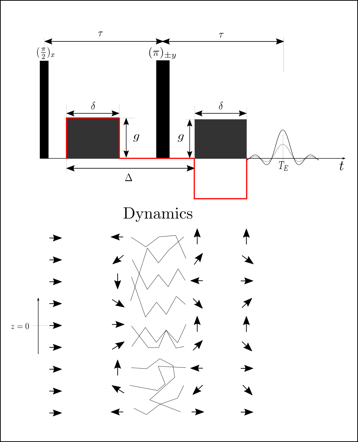
Figure 1: Schematic illustration for the pulse sequence described in Sec. (II.3) when seen in a rotating reference frame with Larmor frequency. Here, the thick red line represents the effective temporal profile of the gradients with amplitude $g$, in which the second gradient polarity is inverted by the $\pi$ RF-pulse; $\delta$, the duration of the gradients; $\Delta$, the gradients spacing. The echo emerges at $T_{E}=2\tau$, when all the spin isochromats come into phase (continuous black line), where $\tau$ is the inter-pulse delay. So any translational motion due to diffusion will cause perturbations to the phase evolution and add an attenuation in the NMR signal (dashed black line).

Diffusion-weighted NMR sequences are made sensitive to diffusion by the addition of magnetic field gradients [28, 29, 30]. Let us consider the diffusive motion of a nucleus in a given pulse sequence, described as follows (see Fig.1). Under a static magnetic field, present throughout all the experiment, the equilibrium longitudinal magnetization is generated. At time $t=0$, an application of a $\pi/2$ RF-pulse gives rise to the transverse magnetization, followed by the formation of the NMR signal, when this disturbance ceases. Then, three subsequent intervals of distinct times can be classified for the diffusion-weighting magnetic field: after signal generation, the gradient is applied during the period $\delta$, which produces an almost instantaneous phase shift for the nucleus, depending on its position (encoding period). After the spatial distinction, they can diffuse in a time interval denoted by $\Delta$ (diffusing interval), which is the time interval that separates the beginning of gradient fields. This period is responsible for the evolution of the spin phase. Finally, a second gradient is applied also with duration $\delta$ (decoding period). If any spin has performed some displacement during the time $\Delta$, a partial phase recovery and an attenuation in the signal will be detected.

The application of a $\pi$ RF-pulse can be taken into account through an effective gradient profile $\textbf{g}^{*}(t)$ for which the magnetization direction is inverted after $\tau$. Since gradients before and after $\pi$ RF-pulse are supposed to be identical, the effective gradient profile $\textbf{g}^{*}(t)$ is antisymmetric with respect to the time $\tau$, i.e.,

$$\mathbf{g^{*}}(\tau-t)=-\mathbf{g^{*}}(t).$$ (13)

In particular, the rephasing condition in Eq.(10) required for echo formation is automatically satisfied. From now on, we stress that the effective gradient profile will be referred to only as $\textbf{g}(t)$.

The possibility of controlling the temporal profile of the gradient field, as well as its amplitude and direction, allows one to obtain different information from the system. The temporal profile is typically trapezoidal in an experiment, but for simplicity in theoretical analysis the rectangular form is assumed with an amplitude given by $|\textbf{g}(t)|=g$, where the simplest case consists of a steady gradient, $\delta=\Delta=\tau$. Finally, one must set the direction to measure the diffusion, denoted by the verse $\hat{\textbf{e}}$, that will be considered fixed. So the effective gradient is

$$\textbf{g}(t)=\begin{cases}\textbf{g},&0\leqslant t\leqslant\tau\\ -\textbf{g},&\tau<t\leqslant 2\tau\end{cases}$$ (14)

Imposing these considerations in Eq.(12), we get

$$\left\langle\frac{\Phi^{2}}{2}\right\rangle=\gamma_{n}^{2}g^{2}\int_{0}^{T_{E}}\int_{0}^{T_{E}}t_{1}t_{2}\left\langle\dot{X}(t_{1})\dot{X}(t_{2})\right\rangle\mathrm{d}t_{1}\mathrm{d}t_{2}.~{}~{}~{}~{}$$ (15)

Where $\hat{\textbf{e}}\cdot\dot{\textbf{r}}=\dot{X}$, so only the correlation between velocity components along the direction $\hat{\textbf{e}}$ of applied gradients takes part. Here, $T_{E}=2\tau$.

III Langevin model

To describe the temporal evolution of a tracer of mass $m$ in contact with a thermal bath of temperature $T$, we will consider a phenomenological model based on a linear generalization of the Langevin equation (GLE) which reads like Newton’s law [14, 21, 22],

$$m\ddot{X}(t)=F_{E}(t)+F_{S}(t)+F(t).$$ (16)

Here, $X=X(t)$ is the displacement of the tracer along a coordinate and $\dot{X}(t)=V(t)$ refers to velocity. The right side of Eq.(16) expresses the balance of forces acting on the tracer:

(i) $F_{E}(t)$ is the external force, which can represent, for example, magnetic, electric fields, Hookean force, etc.

(ii) $F_{S}(t)$ is the generalized Stokes force, with a friction given by a memory kernel $\gamma(t)$, and represents the viscoelastic properties of the medium,

$$F_{S}(t)=-\int_{-\infty}^{t}\gamma(t-t^{\prime})\dot{X}(t^{\prime})~{}\mathrm{d}t^{\prime}.$$ (17)

For the interpretation of experimental trajectories, the initial time can be fixed as $t=0$, so that the causality principle allows one to cut the integrals below 0 in Eq.(17). As a consequence, and due to the linearity of the GLE, standard Laplace transform techniques can be used for a formal solution to the problem.

(iii) $F(t)$ is the rapidly fluctuating thermal force (noise) resulting from molecular collisions. This is the residual force exerted by neighboring molecules - or thermal bath - when the frictional force $F_{S}(t)$ is subtracted.

The thermal force $F(t)$ is a stationary and Gaussian noise. The latter condition implies that its distribution is fully characterized by its mean, which we will consider for simplicity as a zero-mean $\langle F(t)\rangle$ = 0, and the covariance $\langle F(t)F(t^{\prime})\rangle$. In the case of internal noise, the memory kernel is related to the noise correlation function via the fluctuation-dissipation theorem [18],

$$\langle F(t)F(t^{\prime})\rangle=k_{B}T\gamma(|t-t^{\prime}|),$$ (18)

with $\langle\cdots\rangle$ denoting the ensemble average over random realizations of the thermal force $F(t)$, $k_{B}$ being the Boltzmann constant and $T$ the absolute temperature. In this case, the noise and dissipation have the same origin and the system will reach the equilibrium state [18].

In what follows, we will consider $m=1$ and an isolated system, such that $F_{E}(t)=0$, for $t\geq 0$. Combining the above equations, the GLE is given by

$$\ddot{X}(t)+\int_{0}^{t}\gamma(t-t^{\prime})\dot{X}(t^{\prime})~{}\mathrm{d}t^{\prime}=F(t),\quad t\geq 0.$$ (19)

Other forces can be added in Eq.(19), however, it describes the dynamics of a large class of problems, depending on the memory kernel $\gamma(t)$. From now on, since we only deal with times $t\geq 0$, we omit the modulus in the argument of functions.

IV Explicit Solutions

By means of the Laplace transform, one can obtain a formal expression for the displacement $X(t)$ and the velocity $V(t)$ expressed by the GLE in Eq.(19). So, in the Laplace space, we have [31, 32, 33]

$$\hat{X}(s) = \frac{x_{0}}{s}+v_{0}\hat{G}(s)+\hat{G}(s)\hat{F}(s),$$ (20)

$$\hat{V}(s) = v_{0}\hat{g}(s)+\hat{g}(s)\hat{F}(s),$$ (21)

where $\mathcal{L}[F(t)]=\hat{F}(s)$, $\mathcal{L}[X(t)]=\hat{X}(s)$ and $\mathcal{L}[V(t)]=\hat{V}(s)$ gives the Laplace transform of this quantities. Here, $t$ and $s$ are, respectively, the variables in the time domain and Laplace domain. The functions $G(t)$ and $g(t)$ are defined as, respectively,

$$\hat{g}(s) = \frac{1}{s+\hat{\gamma}(s)},$$ (22)

$$\hat{G}(s) = \frac{s^{-1}}{s+\hat{\gamma}(s)},$$ (23)

and represents the relaxation functions. Let’s define another function as

$$\hat{I}(s) = \frac{s^{-2}}{s+\hat{\gamma}(s)},$$ (24)

that will be used later to analyze the displacement correlation function.

The case of thermal initial conditions are considered,

$$x_{0}=0,\,\,\,\,\,\,v_{0}^{2}=k_{B}T,$$ (25)

where $X(0)=x_{0}$ and $V(0)=v_{0}$. Furthermore, for the memory kernel the following assumption should be satisfied

$$\lim_{t\to\infty}\gamma(t)=\lim_{s\to 0}s\hat{\gamma}(s)=0,$$ (26)

where $\mathcal{L}[\gamma(t)](s)=\hat{\gamma}(s)$ is the Laplace transform of $\gamma(t)$.

By applying inverse Laplace transform to Eqs.(20) and (21), it follows,

$$X(t) = \langle X(t)\rangle+\int_{0}^{t}G\left(t-t^{\prime}\right)F\left(t^{\prime}\right)\mathrm{d}t^{\prime},$$ (27)

$$V(t) = \langle V(t)\rangle+\int_{0}^{t}g\left(t-t^{\prime}\right)F\left(t^{\prime}\right)\mathrm{d}t^{\prime},$$ (28)

where,

$$\langle X(t)\rangle = x_{0}+v_{0}G(t),$$ (29)

$$\langle V(t)\rangle = v_{0}g(t).$$ (30)

From the behavior of Eqs. (22)-(24) and its asymptotic limits, one can reveal the diffusion motion features of the particle in a given system by the MSD, time dependent diffusion coefficient and VACF, in the following way [31, 32, 33],

$$\left\langle X^{2}(t)\right\rangle = 2k_{B}TI(t),$$ (31)

$$D(t) = \frac{1}{2}\frac{\mathrm{d}}{\mathrm{d}t}\left\langle X^{2}(t)\right\rangle=k_{B}TG(t),$$ (32)

$$C_{V}(t) = \langle V(t)V(0)\rangle=\left\langle V^{2}(0)\right\rangle g(t).$$ (33)

IV.1 Anomalous diffusion

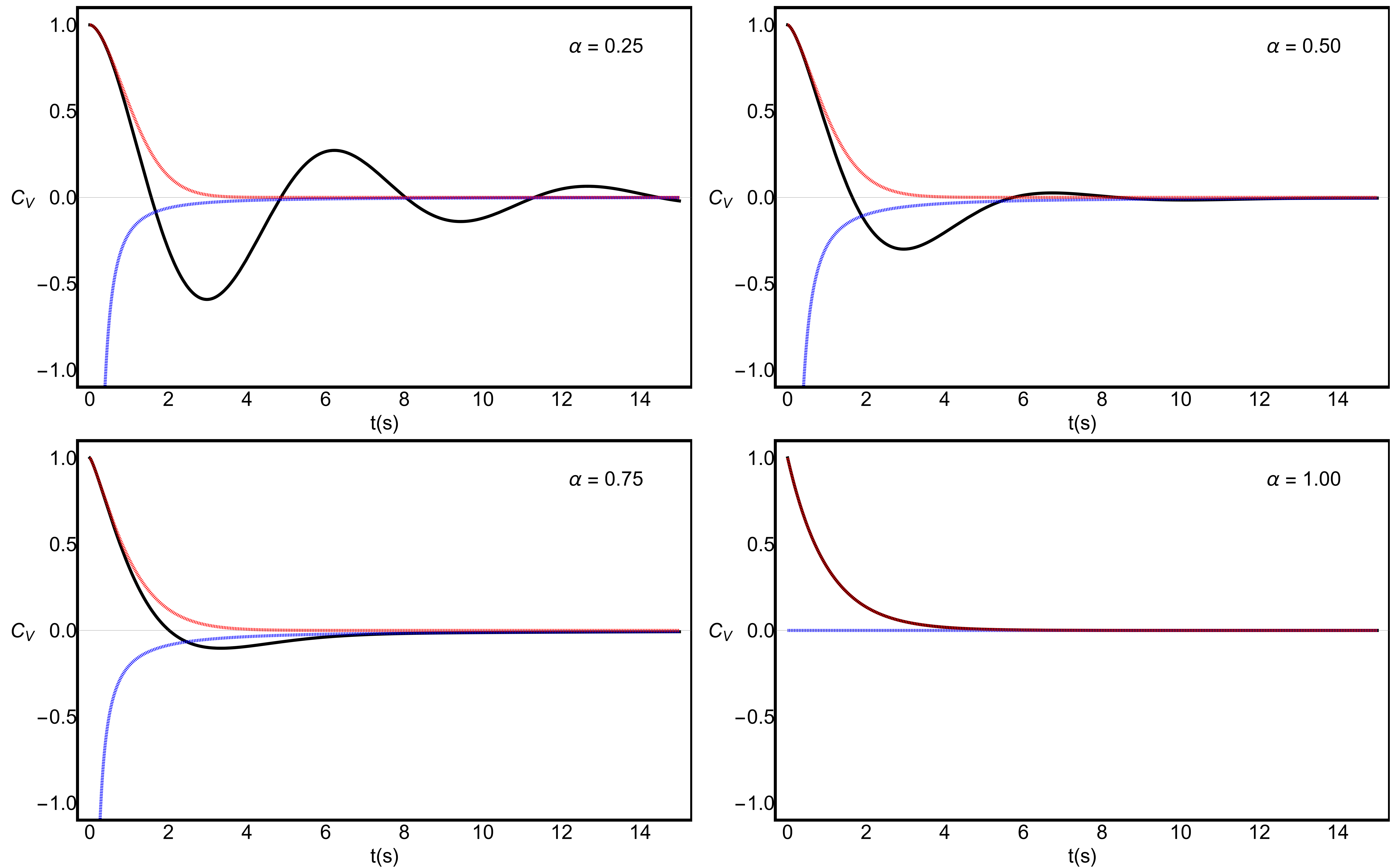
Figure 2: Graphical representation of $C_{V}(t)$ vs time $t$ for different scaling exponents $\alpha$ ($0<\alpha<1$, ranging progressively as $0.25,0.50,0.75,1.00$), for fixed $k_{B}T=1$ and $\gamma_{\alpha}=1$ as described in the text. The figures show the exact relation from Eq.(45) (continuous black line) and its asymptotic representations, the stretched exponential from Eq.(50) valid in the short-time limit (dashed red line) and the power law from Eq.(49) valid in the long-time limit (dashed blue line). Note the different rates of decay for small and large times, where the decay is very fast for short times and very slow for long times. Here, $\alpha=1$ yields a special case of the white noise memory in Eq.(60).

In what follows, we will consider a memory kernel with a power law given by [21, 22],

$$\gamma_{\alpha}(t)=\gamma_{\alpha}\frac{t^{-\alpha}}{\Gamma(1-\alpha)},\quad 0<\alpha<1.$$ (34)

The generalized friction coefficient, $\gamma_{\alpha}$, is independent of time but dependent on the fractional exponent $\alpha$ and $\Gamma(\cdot)$ stand for the Euler-gamma function. This kernel is known to lead to subdiffusive behavior with the scaling exponent $\alpha$ (for $0<\alpha<1$), as will be shown in this section.

Let us now find the relaxation functions $I(t)$, $G(t)$ and $g(t)$ for the memory kernel given in Eq.(34). First, we have that [34]

$$\hat{\gamma}(s)=\mathcal{L}[\gamma(t)](s)=\gamma_{\alpha}s^{\alpha-1}.$$ (35)

So, applying Eq.(35) in (22), we get

$$\hat{g}(s)=\frac{1}{s+\gamma_{\alpha}s^{\alpha-1}}.$$ (36)

The relaxation function $g(t)$ can be found by applying the Laplace inversion of Eq.(36). To do so, we recall that [34],

$$\mathcal{L}\left[t^{\beta-1}\mathrm{E}_{\alpha,\beta}(\lambda t^{\alpha})\right](s)=\frac{s^{\alpha-\beta}}{s^{\alpha}-\lambda},$$ (37)

for $\lambda\in\mathbb{C}$ and $|\lambda s^{-\alpha}|<1$. So, Eq.(36) yields

$$g(t)=\mathcal{L}^{-1}\left[\hat{g}(s)\right](t)=\mathrm{E}_{2-\alpha,1}\left(-\gamma_{\alpha}t^{2-\alpha}\right).$$ (38)

The two parameter Mittag-Leffler (M-L) function is introduced and defined by the series expansion [34],

$$\mathrm{E}_{\alpha,\beta}(z)=\sum_{k=0}^{\infty}\frac{z^{k}}{\Gamma(\alpha k+\beta)},$$ (39)

where $z\in\mathbb{C}$ and $\alpha>0,\beta>0$. Note that $E_{\alpha,1}(z)=E_{\alpha}(z)$.

To proceed, one can use the following identity,

$$\frac{\partial}{\partial t}t^{\beta-1}\mathrm{E}_{\alpha,\beta}\left(\lambda t^{\alpha}\right)=t^{\beta-2}\mathrm{E}_{\alpha,\beta-1}\left(\lambda t^{\alpha}\right),$$ (40)

and evaluate the remaining relaxation functions in Eqs.(23) and (24) from Eq.(36),

$$G(t) = t\mathrm{E}_{2-\alpha,2}\left(-\gamma_{\alpha}t^{2-\alpha}\right),$$ (41)

$$I(t) = t^{2}\mathrm{E}_{2-\alpha,3}\left(-\gamma_{\alpha}t^{2-\alpha}\right).$$ (42)

The displacement and velocity in Eqs.(27) and (28) are obtained from Eqs.(38), (41), and the initial conditions given by (25). Also from the above relations, the Eqs.(31)-(33) yields,

$$\left\langle X^{2}(t)\right\rangle = 2k_{B}Tt^{2}\mathrm{E}_{2-\alpha,3}\left(-\gamma_{\alpha}t^{2-\alpha}\right),$$ (43)

$$D(t) = k_{B}Tt\mathrm{E}_{2-\alpha,2}\left(-\gamma_{\alpha}t^{2-\alpha}\right),$$ (44)

$$C_{V}(t) = k_{B}T\mathrm{E}_{2-\alpha,1}\left(-\gamma_{\alpha}t^{2-\alpha}\right).$$ (45)

The asymptotic behavior of the relaxation functions relies on the analysis of M-L function [34],

$$\mathrm{E}_{\alpha,\beta}\left(-\gamma_{\alpha}t^{\alpha}\right)\simeq\begin{cases}\frac{1}{\Gamma(\beta)}-\frac{\gamma_{\alpha}t^{\alpha}}{\Gamma(\alpha+\beta)},&\text{ as }|\gamma_{\alpha}t^{\alpha}|<<1\\ \frac{t^{-\alpha}}{\gamma_{\alpha}\Gamma(\beta-\alpha)},&\text{ as }|\gamma_{\alpha}t^{\alpha}|>>1\end{cases}$$ (46)

Introducing these asymptotic expansion in Eqs.(43)-(45), we get,

$$\left\langle X^{2}(t)\right\rangle\simeq 2k_{B}T\begin{cases}\frac{t^{2}}{\Gamma(3)}-\frac{\gamma_{\alpha}t^{4-\alpha}}{\Gamma(5-\alpha)},&\text{ as }|\gamma_{\alpha}t^{2-\alpha}|<<1\\ \frac{1}{\gamma_{\alpha}}\frac{t^{\alpha}}{\Gamma(1+\alpha)},&\text{ as }|\gamma_{\alpha}t^{2-\alpha}|>>1\end{cases}$$ (47)

$$D(t)\simeq k_{B}T\begin{cases}\frac{t}{\Gamma(2)}-\frac{\gamma_{\alpha}t^{3-\alpha}}{\Gamma(4-\alpha)},&\text{ as }|\gamma_{\alpha}t^{2-\alpha}|<<1\\ \frac{1}{\gamma_{\alpha}}\frac{t^{\alpha-1}}{\Gamma(\alpha)},&\text{ as }|\gamma_{\alpha}t^{2-\alpha}|>>1\end{cases}$$ (48)

$$C_{V}(t)\simeq k_{B}T\begin{cases}\frac{1}{\Gamma(1)}-\frac{\gamma_{\alpha}t^{2-\alpha}}{\Gamma(3-\alpha)},&\text{ as }|\gamma_{\alpha}t^{2-\alpha}|<<1\\ \frac{1}{\gamma_{\alpha}}\frac{t^{\alpha-2}}{\Gamma(\alpha-1)},&\text{ as }|\gamma_{\alpha}t^{2-\alpha}|>>1\end{cases}$$ (49)

Where we observe power law behavior for Eq.(47) in the long-time regime (anomalous diffusion), a slower diffusion (subdiffusive behavior) for $0<\alpha<1$, with the generalized diffusion coefficient $D_{\alpha}=k_{B}T/\gamma_{\alpha}$ [21, 22].

In this paper, we are mainly interested in calculating the NMR signal attenuation by the VACF. Graphical representations of the exact VACF, Eq.(45), and its asymptotic limits, Eqs.(49), in the case of thermal initial conditions and different values of the parameter $\alpha$ are given in Fig.(2), for $0<\alpha<1$. We illustrate how the scaling exponent $\alpha$ influences the behavior of the VACF, the other parameters being kept fixed. As a consequence from Fig.(2), the VACF interpolates, for intermediate time $t$, between the stretched exponential, expressed from Eq.(49) in the convergent power series representation,

$$C_{V}(t)\simeq k_{B}T\exp\left\{-\frac{\gamma_{\alpha}t^{2-\alpha}}{\Gamma(3-\alpha)}\right\}, \text{ as }|\gamma_{\alpha}t^{2-\alpha}|<<1~{}~{}~{}~{}$$ (50)

and the negative power law. For small time $t$, the stretched exponential models the very fast decay, whereas for large time $t$ it decays with a long negative tail.

IV.2 Normal diffusion

The standard Langevin equation for normal diffusion, i.e., without memory, is obtained when $\alpha=1$ in Eq.(34). In that case, one uses $\gamma_{1}(t)=2\gamma_{1}\delta(t)$ to retrieve the instantaneous Stokes force $-\gamma_{1}\dot{X}(t)$, where $\delta(t)$ is the Dirac distribution which corresponds to a white noise. So the GLE in Eq.(19) yields a special case of the standard Brownian motion and the classical Langevin equation,

$$\ddot{X}(t)+\gamma_{1}(t)\dot{X}(t)=F(t),\quad t\geq 0.$$ (51)

The results for the relaxation functions, Eqs.(22)-(24), arises in a similar manner of Sec. IV.1. From that, we get

$$g(t) = \mathrm{e}^{-\gamma_{1}t},$$ (52)

$$G(t) = (1-\mathrm{e}^{-\gamma_{1}t})/\gamma_{1},$$ (53)

$$I(t) = (\gamma_{1}t-1+\mathrm{e}^{-\gamma_{1}t})/\gamma_{1}^{2},$$ (54)

and for Eqs.(31)-(33),

$$\left\langle X^{2}(t)\right\rangle = 2k_{B}T(\gamma_{1}t-1+\mathrm{e}^{-\gamma_{1}t})/\gamma_{1}^{2},$$ (55)

$$D(t) = k_{B}T(1-\mathrm{e}^{-\gamma_{1}t})/\gamma_{1},$$ (56)

$$C_{V}(t) = k_{B}T\mathrm{e}^{-\gamma_{1}t},$$ (57)

where we used that $E_{1,1}(z)=\mathrm{e}^{z}$, $E_{1,2}(z)=\frac{\mathrm{e}^{z}-1}{z}$, and $E_{1,3}(z)=\frac{\mathrm{e}^{z}-1-z}{z^{2}}$ [34].

The asymptotic behavior from Eqs.(46) of the above relations give us,

$$\left\langle X^{2}(t)\right\rangle\simeq 2k_{B}T\begin{cases}\frac{t^{2}}{\Gamma(3)}-\frac{\gamma_{1}t^{3}}{\Gamma(4)},&\text{ as }|\gamma_{1}t|<<1\\ \frac{1}{\gamma_{1}}\frac{t}{\Gamma(2)},&\text{ as }|\gamma_{1}t|>>1\end{cases}$$ (58)

$$D(t)\simeq k_{B}T\begin{cases}\frac{t}{\Gamma(2)}-\frac{\gamma_{1}t^{2}}{\Gamma(3)},&\text{ as }|\gamma_{1}t|<<1\\ \frac{1}{\gamma_{1}},&\text{ as }|\gamma_{1}t|>>1\end{cases}$$ (59)

$$C_{V}(t)\simeq k_{B}T\begin{cases}\frac{1}{\Gamma(1)}-\frac{\gamma_{1}t}{\Gamma(2)},&\text{ as }|\gamma_{1}t|<<1\\ 0,&\text{ as }|\gamma_{1}t|>>1\end{cases}$$ (60)

Where we observe normal diffusive behavior for Eq.(58) in the long-time regime, as we expected.

IV.3 NMR signal attenuation

We can now use the results from previous section to evaluate the NMR signal attenuation due do diffusion in both anomalous and normal cases. So, from Eq.(15) and (45), we have

$$\left\langle\frac{\Phi^{2}}{2}\right\rangle=\gamma_{n}^{2}g^{2}\mathrm{\textbf{I}},$$ (61)

with the following integral to be solved,

I $$= k_{B}T$$ (62)

$$\int_{0}^{T_{E}}\int_{0}^{T_{E}}t_{1}t_{2}\mathrm{E}_{2-\alpha,1}\left(-\gamma_{\alpha}|t_{1}-t_{2}|^{2-\alpha}\right)\mathrm{d}t_{1}\mathrm{d}t_{2}.~{}~{}~{}~{}~{}~{}$$

The Eq.(62) may be integrated (see, e.g, [34]), and one obtains the exacts results for the effective gradient in Eq.(14),

$$\mathrm{\textbf{I}}=k_{B}T\begin{cases}\tau^{4}[2\mathrm{E}_{2-\alpha,5}\left(-\gamma_{\alpha}\tau^{2-\alpha}\right)],&t=\tau\\ \tau^{4}[2^{4}\mathrm{E}_{2-\alpha,5}\left(-\gamma_{\alpha}(2\tau)^{2-\alpha}\right)\\ \quad-2^{2}\mathrm{E}_{2-\alpha,5}\left(-\gamma_{\alpha}\tau^{2-\alpha}\right)],&t=2\tau\end{cases}$$ (63)

The exact attenuation in Eq.(8) is then given by Eqs.(63) and (61). In the long-time limit yields,

$$E\simeq\begin{cases}\exp\left\{-\frac{2}{\Gamma(\alpha+3)}\gamma_{n}^{2}g^{2}D_{\alpha}\tau^{\alpha+2}\right\},&t=\tau\\ \exp\left\{-\frac{\left(1-1/2^{\alpha}\right)}{\Gamma(\alpha+3)}\gamma_{n}^{2}g^{2}D_{\alpha}T_{E}^{\alpha+2}\right\},&t=2\tau\end{cases}$$ (64)

Here, in Eq.(64) we see that when the system is driven by the memory kernel in Eq.(34), the fractional exponent $\alpha$ plays a role in the NMR signal attenuation. Note that the relation (64) agrees with the one obtained by Kärger et al. approach [35] for the case expressed by Eq.(34).

At last, for normal diffusion ($\alpha$ = 1) in Eq.(64),

$$E=\begin{cases}\exp\left\{-\frac{1}{3}\gamma_{n}^{2}g^{2}D\tau^{3}\right\},&t=\tau\\ \exp\left\{-\frac{1}{12}\gamma_{n}^{2}g^{2}DT_{E}^{3}\right\},&t=2\tau\end{cases}$$ (65)

one retrieves the Hanh echo [6] expected result of the NMR signal attenuation due to normal diffusion as in Eq.(3).

V Conclusions Remarks

In the present work, with the application of a magnetic field gradient, it was possible to encode the nuclei trajectories. We investigate the underlying stochastic processes using a phenomenological description provide by a generalized Langevin equation (GLE). While in simple systems the memory friction kernel yields a white noise, in complex environments the picture is different, exhibiting some form of memory. We have chosen a memory kernel that decays as a power law with the scaling exponent $\alpha$, which leads to anomalous behavior. Namely, the relaxation functions are of a power law type and were expressed in terms of generalized Mittag-Leffler functions and their derivatives. The asymptotic behavior of these quantities was obtained and reveals, in the long-time regime, subdiffusion behavior for $0<\alpha<1$.

We have shown how one can apply the results from this approach to evaluate the Nuclear Magnetic Resonance (NMR) signal attenuation due to diffusion as a function of the velocity autocorrelation function (VACF), a relevant quantity that provides details of molecular dynamics and that can be measured in the laboratory [36]. Here, we consider acquisitions made with a steady gradient and within the framework of the Gaussian phase approximation (GPA). We emphasize that other gradient temporal profiles and pulse sequences could also be used but the above case capture all the essential features of the gradient NMR experiment.

On the one hand, we demonstrate the advantages of using the GLE approach in theoretical studies of anomalous diffusion. On the other hand, the mathematical description allows one to evaluate and properly interpret, in the long-time diffusion regime, the expression for diffusion-based NMR experiments. The choice of a memory kernel that decays as a power law allows one to perform the calculation analytically, illustrate the emergence of fractional order exponential decay in the NMR signal amplitude and retrieve the classic result from Hanh echo [6]. Finally, we conclude that the solutions may also be extended to describe the dynamics of a broad class of systems, depending on the memory kernel $\gamma(t)$ [21, 22]. So we expect the obtained results from this framework to be useful for a better description of experimental data.

References

- Abragam [1961] A. Abragam, The Principles of Nuclear Magnetism (Oxford Univ. Press, London, 1961).
- Callaghan [1991] P. T. Callaghan, Principles of Nuclear Magnetic Resonance Microscopy (Oxford Univ. Press, Oxford, 1991).
- Callaghan [2011] P. T. Callaghan, Translational Dynamics and Magnetic Resonance: Principles of Pulsed Gradient Spin Echo NMR (Oxford University Press, New York, 2011).
- Price [2009] W. S. Price, NMR studies of translational motion: principles and application (Cambridge University Press, 2009).
- Kimmich [2011] R. Kimmich, NMR: tomography, diffusometry, relaxometry (Springer Science & Business Media, 2011).
- Hahn [1950] E. L. Hahn, Phys. Rev. 80, 580 (1950).
- Grebenkov [2007] D. S. Grebenkov, Rev. Mod. Phys. 79, 1077 (2007).
- Bloch [1946] F. Bloch, Phys. Rev. 70, 460 (1946).
- Purcell et al. [1946] E. M. Purcell, H. C. Torrey, and R. V. Pound, Phys. Rev. 69, 37 (1946).
- Price [1997] W. S. Price, Concepts Magn. Reson. 9, 299 (1997).
- Stallmach and Galvosas [2007] F. Stallmach and P. Galvosas, Annu. Rep. NMR Spectrosc. 61, 51 (2007).
- Reif [2009] F. Reif, Fundamentals of statistical and thermal physics (Waveland Press, 2009).
- Chandrasekhar [1943] S. Chandrasekhar, Rev. Mod. Phys. 15, 1 (1943).
- van Kampen [1992] N. G. van Kampen, Stochastic Processes in Physics and Chemistry (North-Holland, Amsterdam, 1992).
- Nelson [1967] E. Nelson, Dynamical Theories of Brownian Motion (Princeton University Press, Princeton, 1967).
- Metzler and Klafter [2000] R. Metzler and J. Klafter, Phys. Rep. 339, 1 (2000).
- Lutz [2001] E. Lutz, Phys. Rev. E 64, 051106 (2001).
- Kubo et al. [1985] R. Kubo, M. Toda, and N. Hashitsume, Statistical Physics II. Nonequilibrium Statistical Mechanics (Springer, Berlin, 1985).
- Langevin [1908] P. Langevin, C. R. Acad. Sci. (Paris) 146, 530 (1908).
- Coffey et al. [2004] W. T. Coffey, Y. P. Kalmykov, and J. T. Waldron, The Langevin equation: With Applications to Stochastic Problems in Physics, Chemistry and Electrical Engineering (World Scientific, Singapore, 2004).
- Grebenkov et al. [2013] D. S. Grebenkov, M. Vahabi, E. Bertseva, L. Forró, and S. Jeney, Phys. Rev. E 88, 040701(R) (2013).
- Grebenkov and Vahabi [2014] D. S. Grebenkov and M. Vahabi, Phys. Rev. E 89, 012130 (2014).
- Cooke et al. [2009] J. M. Cooke, Y. P. Kalmykov, W. T. Coffey, and C. M. Kerskens, Phys. Rev. E 80, 061102 (2009).
- Lisỳ and Tóthová [2017a] V. Lisỳ and J. Tóthová, J. Magn. Reson. 276, 1 (2017a).
- Lisỳ and Tóthová [2017b] V. Lisỳ and J. Tóthová, J. Mol. Liq. 234, 182 (2017b).
- Lisỳ and Tóthová [2018] V. Lisỳ and J. Tóthová, Physica A 494, 200 (2018).
- Callaghan and Stepišnik [1996] P. T. Callaghan and J. Stepišnik, Adv. Magn. and Opt. Reson. 19, 325 (1996).
- Carr and Purcell [1954] H. Y. Carr and E. M. Purcell, Phys. Rev. 94, 630 (1954).
- Torrey [1956] H. C. Torrey, Phys. Rev. 104, 563 (1956).
- Stejskal and Tanner [1965] E. O. Stejskal and J. E. Tanner, J. Chem. Phys. 42, 288 (1965).
- Viñales and Despósito [2006] A. D. Viñales and M. A. Despósito, Phys. Rev. E 73, 016111 (2006).
- Viñales and Despósito [2007] A. D. Viñales and M. A. Despósito, Phys. Rev. E 75, 042102 (2007).
- Despósito and Viñales [2009] M. A. Despósito and A. D. Viñales, Phys. Rev. E 80, 021111 (2009).
- Podlubny [1998] I. Podlubny, Fractional differential equations: an introduction to fractional derivatives, fractional differential equations, to methods of their solution and some of their applications (Elsevier, 1998).
- Kärger et al. [1988] J. Kärger, H. Pfeifer, and G. Vojta, Phys. Rev. A 37, 4514 (1988).
- Stepišnik and Callaghan [2000] J. Stepišnik and P. T. Callaghan, Condens. Matter 292, 296 (2000).