Local-realistic Bohmian trajectories: a non-Bohmian approach to wave-particle duality

Abstract

We present a local-realistic description of both wave-particle duality and Bohmian trajectories. Our approach is relativistic and based on Hamilton’s principle of classical mechanics, but departs from its standard setting in two respects. First, we address an ensemble of extremal curves, the so-called Mayer field, instead of focusing on a single extremal curve. Second, we assume that there is a scale, below which we can only probabilistically assess which extremal curve in the ensemble is actually realized. The continuity equation ruling the conservation of probability represents a subsidiary condition for Hamilton’s principle. As a consequence, the ensemble of extremals acquires a dynamics that is ruled by Maxwell equations. These equations are thus shown to also rule some non-electromagnetic phenomena. While particles follow well-defined trajectories, the field of extremals can display wave behavior.

Bohmian trajectories (BT) represent a particle’s feature that can be derived from Schrödinger’s wave equation. Once dubbed as “surreal”, such a labeling has been rendered inappropriate by recent experiments kocsis2011 ; mahler2016 ; Xiao2017 , in which single-photon BT were registered through weak-value measurements aharonov . There were two main reasons to see BT as surreal. First, the orthodox (Copenhagen) interpretation of quantum mechanics (QM) forbids assigning physical reality to particle trajectories, as these presuppose well-defined positions and velocities. Second, BT were numerically calculated philippidis and experimentally measured for a two-slit Young setup, in which they displayed curvilinear motion. BT are therefore at odds with the principle of inertia cohen2020 . To be sure, the physical interpretation of BT is still open to debate englert1992 ; scully1998 ; dewdney1993 ; durr1993 ; englert1993 ; wiseman2003 ; schleich2013 ; wu2013 ; bliokh ; jooya2016 ; Tastevin2018 ; yu2018 ; cheng2018 ; douguet2018 ; Xiao2019 ; li2021 , but the very debate shows that the Copenhagen interpretation has not really established itself as a full-fledged paradigm that replaced the classical one. The quantum formalism can actually be used without adhering to the Copenhagen interpretation. Perhaps most physicists keep thinking of an electron as a well-localized particle that moves with a well-defined velocity, thereby adopting a realist view as long as it is not necessary to deal with foundational issues. The latter have lately sparked interest in a community that includes application-oriented scientists. This is because the so-called “quantum advantage” is claimed to derive from unique quantum features, such as coherent state-superposition and entanglement. It is thus important to make sure that it is impossible to employ conventional technology, which is based on classical physics, in order to implement quantum algorithms in an efficient and scalable way. Impossibility claims should however rest on a firm scientific ground rather than on ideological views.

Wave-particle duality (WPD) is also seen as a distinctive quantum feature. Indeed, Feynman famously said feynman that WPD is a phenomenon that “is impossible, absolutely impossible, to explain in any classical way”. Feynman’s claim does not rest on a firm, scientific basis. Not even Bell’s theorem mermin1993 could provide such a basis for a claim that is representative of a philosophical view rather than a demonstrable proposition. Said view arose in a cultural environment that was hostile to rationalism and causality in general, including their manifestation in classical physics meyenn . The extraordinary scientific stature of people like Bohr, Heisenberg, Pauli, Dirac, Born and other developers of QM, contributed much to disseminate their philosophical view and to make it the prevailing one. It is by now common place to say that WPD ascribes mutually exclusive properties to one and the same physical object. We are, however, not compelled to subscribe such a view selleri ; aharonov2017 . We may ascribe particle-like properties to an electron, say, while wave-like properties characterize the probability to find the electron at a given place and time. Electron and probability are two different concepts. One of them may be characterized by particle features, and the other by wave features. Only particular, historical circumstances that defined the European environment of the early twentieth century led physicists to see a paradox where there is none. In economics, for instance, nobody sees a paradox in establishing mathematical – deterministic or stochastic – models for some commodities market, while recognizing the unpredictable, free-will behavior of the individuals who drive this market.

There are two main lines of research regarding WPD. One of them is concerned with its quantification and started in 1979 with the work of Wootters and Zurek wooters , which gave rise to much development in this field wooters ; scully1991 ; jaeger ; englert1996 ; jakob2010 ; Coles2014 ; qian2016 ; eberly2017 ; qian2018 ; norrman2020 ; miranda2021 ; qureshi2021 ; qian0 . The other research line started in the mid-1920s and was concerned with a realistic interpretation of the Schrödinger equation. A first attempt was that of Madelung holland1993 , which was further developed by Bohm bohm and others. This line of research led to the BT that we address here. We will present an alternative approach to that of Madelung, de Broglie and Bohm holland1993 , an approach that fully fits within the classical framework. In particular, we present a local-realistic description of the two-slit experiment. We do this not for the sake of proving Feynman wrong, but to explore possible new avenues towards a better understanding of the quantum-classical boundary haroche2013 ; nassar2013 . Schrödinger’s equation shows how probability, a rather abstract and – in its Bayesian formulation – subjective concept, can nonetheless be subjected to deterministic dynamics, as though it were a physical object. We show here that classical physics admits a similar treatment. Indeed, from Hamilton’s principle and the conservation of probability, one can derive Maxwell-like equations that rule the motion of a particle and its associated probability density.

Bohmian mechanics and classical optics

As is well-known, de Broglie prompted Schrödinger to find his equation. Schrödinger’s equation was intended to be for material particles what the wave equation was for optical phenomena. The optical wave equation can be derived from Maxwell equations, the short-wave limit of which leads to ray optics. The latter can alternatively be based on Fermat’s principle, which is the optical counterpart of Hamilton’s principle in mechanics. In his quest to find the equivalent of the optical wave equation in mechanics, Schrödinger postulated his equation. Its precise link to classical mechanics remains undetermined.

Let us first discuss the connection between the optical wave equation and Schrödinger’s equation. In scalar wave optics saleh ; wolf , light propagation in vacuum is described by a real function $u(\mathbf{r},t)$, which satisfies $(\partial^{2}/c^{2}\partial t^{2}-\nabla^{2})u=0$. The optical intensity is given by $I(\mathbf{r},t)=2\langle u^{2}(\mathbf{r},t)\rangle$, where angular brackets denote averaging over a time much longer than any optical cycle. In the monochromatic case, it is convenient to introduce a complex function $U(\mathbf{r},t)=U(\mathbf{r})e^{i\omega t}$, such that $u(\mathbf{r},t)=\operatorname{Re}U(\mathbf{r},t)$. Then, $I(\mathbf{r})=|U(\mathbf{r})|^{2}$. If light propagates in a medium of refractive index $n(\mathbf{r})$, the wave equation reads

$$\left(\frac{1}{v^{2}}\frac{\partial^{2}}{\partial t^{2}}-\nabla^{2}\right)U(\mathbf{r},t)=0,$$ (1)

with $v=c/n$. On setting $U(\mathbf{r},t)=U(\mathbf{r})e^{i\omega t}$ in Eq. (1), we get the Helmholtz equation

$$\nabla^{2}U(\mathbf{r})+k^{2}U(\mathbf{r})=0,$$ (2)

with $k=n\omega/c$. Let us set $U(\mathbf{r})=a(\mathbf{r})\exp[-ik_{0}\tilde{S}(\mathbf{r})]$, with $k_{0}=\omega/c$, the wave number in vacuum. Separating real and imaginary parts of Eq. (2) yields

$$|\nabla\tilde{S}|^{2}-n^{2}-\lambdabar^{2}\frac{\nabla^{2}a}{a} = 0$$ (3)

$$2\bm{\nabla}a\cdot\bm{\nabla}\tilde{S}+a\nabla^{2}\tilde{S} = 0,$$ (4)

where $\lambdabar=1/k_{0}$. If $a(\mathbf{r})$ varies slowly over distances in the order of $\lambdabar$, we can neglect the second term on the right-hand side of Eq. (3), thereby obtaining the eikonal equation: $|\nabla\tilde{S}|^{2}=n^{2}$. This is the domain of ray optics. Rays are defined as trajectories orthogonal to the level surfaces $\tilde{S}(\mathbf{r})=\text{const}$. Setting the arc-length $s$ as curve parameter, light rays are solutions of the differential equation

$$\frac{d\mathbf{r}}{ds}=\frac{1}{n(\mathbf{r}(s))}\bm{\nabla}\tilde{S}(\mathbf{r}(s)).$$ (5)

Let us now turn to the Schrödinger equation: $i\hbar\partial\psi/\partial t=-\hbar^{2}\nabla^{2}\psi/2m+V(\mathbf{r})\psi$. Setting $\Psi(\mathbf{r},t)=R(\mathbf{r},t)\exp{(iS(\mathbf{r},t)/\hbar)}$ and splitting real and imaginary parts gives

$$\frac{\partial S}{\partial t}+\frac{|\nabla S|^{2}}{2m}+V-\frac{\hbar^{2}}{2m}\frac{\nabla^{2}R}{R} = 0,$$ (6)

$$\frac{\partial R^{2}}{\partial t}+\bm{\nabla}\cdot\left(R^{2}\frac{\bm{\nabla}S}{m}\right) = 0.$$ (7)

For $R=R(\mathbf{r})$ and $S(\mathbf{r},t)=-Et+S(\mathbf{r})$, the above equations reduce to Eqs. (3) and (4), with the replacements $S/\hbar\rightarrow\tilde{S}/\lambdabar$, $\hbar R^{2}/m\rightarrow\lambdabar a^{2}$ and $2m(E-V)/\hbar^{2}\rightarrow n/\lambdabar^{2}$. Eq. (6) is the Hamilton-Jacobi equation with the “quantum potential” $Q=-\hbar^{2}\nabla^{2}R/(2mR)$ added to $V$. Eq. (7) is a continuity equation for the probability density $\rho=R^{2}$ and probability current $\mathbf{j}=R^{2}\bm{\nabla}S/m$. From $S(\mathbf{r})$, one obtains particle trajectories by integrating

$$\frac{d\mathbf{r}}{dt}=\frac{1}{m}\bm{\nabla}S(\mathbf{r}(t)).$$ (8)

Eqs. (6), (7) and (8) are the basis of Bohm’s reformulation of Schrödinger’s wave mechanics. Finding $S(\mathbf{r})$ in the case of Young’s double-slit configuration is a difficult task. A more viable approach is to get $S$ and $R$ from a solution $\Psi(\mathbf{r})=R(\mathbf{r})\exp{(iS(\mathbf{r})/\hbar)}$ of the time-independent Schrödinger equation for free particles and double-slit boundary conditions. On using Feynman’s path integral method, Philippidis et al. philippidis numerically obtained BT with data taken from experiments performed by Jönsson jonsson . It is important to notice that these experiments did not test the Schrödinger equation itself, but a consequence of it, Helmholtz’s equation (2).

Bohm’s approach provides a realistic and deterministic framework whose predictions coincide with those of QM. However, the price paid for this deterministic version is a drastic departure from the most basic tenets of classical physics. Particles following BT display curvilinear motion, even though there is no external force acting on them. Curvilinear motion is caused by $Q$, the quantum potential. This potential, besides being non-local, stems from the particle itself through its associated “pilot-wave”. This amounts to endow probability (amplitudes) with physical existence. Hence, by adopting Bohm’s approach, we must accept self-action as a matter of principle, something that is even more at odds with the basic tenets of classical physics than QM itself.

No departure from the classical formalism is needed to explain Jönsson’s interference patterns and BT. A classical description may include both particle-like features and wave-like features. In classical mechanics, particles move along extremal curves of an action principle: $\delta\int L(x,\dot{x})ds=0$. An extremal curve is a solution of the Euler-Lagrange equations for the Lagrangian $L(x,\dot{x})$. The variational problem, which consists in finding an extremal curve, in fact requires finding a whole set of extremals. The sought-after extremal curve must be in fact a member of a whole field of such curves. This is the imbedding theorem in the calculus of variations bliss ; Caratheodory ; Rund , basically a consequence of continuity assumptions.

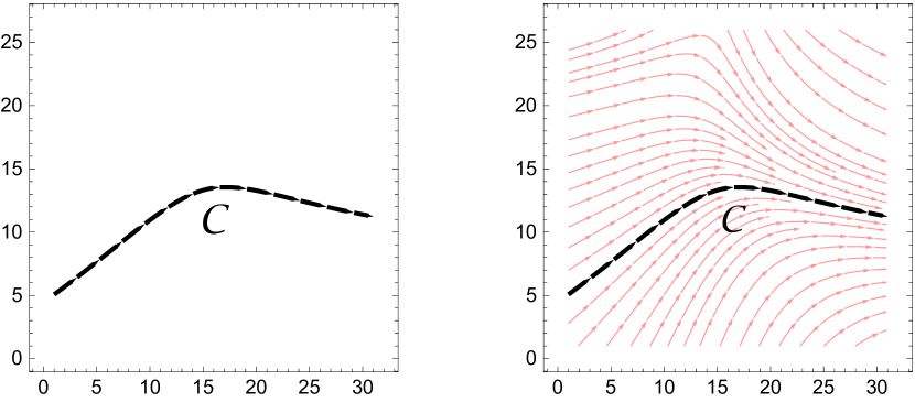
Figure 1: Left panel: curve $C$ renders $\int L(x,\dot{x})ds$ extremal. One usually focuses on a single extremal curve, even though this curve must be embedded in a whole family of extremals. Right panel: the complete picture. $C$ is just one member of a whole family of curves, whose collective behavior is ruled by field equations.

The left panel of Fig. (1) illustrates the usual approach, in which a single extremal is addressed. The right panel shows instead the whole picture: the sought-after extremal exists only within a Mayer field bliss , a “pilot-field”, as we may call it. Depending on the boundary conditions, one and the same Lagrangian can lead to different fields. A screen with two open slits is not the same as a screen with only one open slit. A particle that goes through one slit can “know” whether the other slit is open or not, because its trajectory belongs to a field whose structure depends on whether the two slits are open or not. While it hardly makes sense to say that a single particle interferes with itself, a field may well develop wave dynamics. Interference phenomena are thus possible for fields of extremals. A two-slit scenario can lead to an interference pattern. By sending and detecting one particle after the other, we can exhibit such a pattern. There is no conflict between the two features that show up here: particle and wave may coexist.

Carathéodory’s “royal road”

The foregoing statements derive from Hamilton’s principle: $\delta I\equiv\delta\int L(x,\dot{x})ds=0$. The existence of the Mayer field imposes some integrability conditions. Carathéodory’s “royal road” to the Calculus of Variations Caratheodory leads at once to Euler-Lagrange, Hamilton and Hamilton-Jacobi equations.

Let us summarize Carathéodory’s approach, focussing on a relativistic formulation, whose action principle has the form $\delta\int L(x,\dot{x})ds=0$. In Carathéodory’s approach, $L(x,\dot{x})$ is written as a function of $x$ and the velocity-field $v(x)$: $L=L(x,v(x))$. Extremal curves $\mathcal{C}$ are solutions of

$$\frac{dx^{\mu}(s)}{ds}=v^{\mu}(x(s)).$$ (9)

We seek for a field $v(x)$ whose integral curves render $\int Lds$ extremal. To this end, we introduce an auxiliary function $S(x)$ and require that the following, fundamental equations are satisfied Caratheodory ; Rund ; supp :

$$L(x,v)-v^{\mu}(x)\partial_{\mu}S(x) = 0$$ (10)

$$\partial L(x,v)/\partial v^{\mu} = \partial S/\partial x^{\mu}.$$ (11)

On account of the integrability conditions $\partial^{2}S/\partial x^{\mu}\partial x^{\nu}=\partial^{2}S/\partial x^{\nu}\partial x^{\mu}$, it follows from (11) that

$$\frac{\partial}{\partial x^{\mu}}\left(\frac{\partial L(x,v(x))}{\partial v^{\nu}}\right)-\frac{\partial}{\partial x^{\nu}}\left(\frac{\partial L(x,v(x))}{\partial v^{\mu}}\right)=0.$$ (12)

From Eq. (12), we can get the equations of motion supp . Carathéodory’s formulation addresses local properties, rather than some particular extremal curve. The latter can be singled out by choosing initial values $x^{\mu}(s_{0})=x^{\mu}_{0}$ when solving Eq. (9). We will consider situations for which $x^{\mu}_{0}$ occurs with some probability and introduce a normalized probability distribution $\rho(x^{\mu})\geq 0$, with $\int\rho(x^{\mu})d^{4}x=1$. Notice that this is not the standard framework of statistical mechanics, where $\rho$ depends on both position and momentum: $\rho(x^{\mu},p_{\mu})$.

Two local-realistic descriptions

Let us consider now a free particle. Its Lorentz invariant Lagrangian reads

$$L(x,v)=mc(\eta_{\mu\nu}v^{\mu}v^{\nu})^{1/2}\equiv mc\,\phi,$$ (13)

where $\eta_{\mu\nu}=\operatorname{diag}(+1,-1,-1,-1)$ is the Minkowski metric tensor. It holds $\partial L/\partial v^{\nu}=mcv_{\nu}/\phi=\partial S/\partial x^{\nu}$. Given $v^{\nu}$, we can find a $\rho(x)$, such that $\partial_{\nu}(\rho v^{\nu})=0$. Indeed, this “continuity equation” can be written in the form $v^{\nu}\partial_{\nu}\ln\rho=-\partial_{\nu}v^{\nu}$, which has a solution $\rho(x)$ for fairly general boundary conditions. Moreover, the integrability conditions $\partial^{2}S/\partial x^{\mu}\partial x^{\nu}=\partial^{2}S/\partial x^{\nu}\partial x^{\mu}$ lead to

$$\partial_{\mu}w_{\nu}-\partial_{\nu}w_{\mu}=0,$$ (14)

with $w_{\nu}=v_{\nu}/\phi$. From $w^{\mu}w_{\mu}=1$, it follows that $w^{\mu}\partial_{\nu}w_{\mu}=0$. Thus, Eq. (14) implies $w^{\mu}\partial_{\mu}w_{\nu}=0$, which means that $dw_{\nu}/ds=0$, i.e, the extremals are straight lines. This corresponds to an idealized description, in which measurement devices have infinite resolution and particles have exact, sharply defined locations $x^{\mu}$.

First probabilistic model

Assume now that there is a scale, below which we can assign locations only probabilistically. Both $v^{\nu}(x)$ and $\rho(x)$ must now be determined together. Assume further that $\rho=n_{0}c/\phi$, with $n_{0}$ a constant providing dimensional consistency. $\rho(x)$ is thus given by the vector-norm $v_{\nu}(x)v^{\nu}(x)$, a possible quantifier for the “density” of the field-lines. Eq. (14) now reads $\partial_{\mu}(\rho v_{\nu})-\partial_{\nu}(\rho v_{\mu})=0$. Using $\partial^{\mu}(\rho v_{\mu})=0$, we get $\partial^{\mu}\partial_{\mu}(\rho v_{\nu})-\partial^{\mu}\partial_{\nu}(\rho v_{\mu})=\partial^{\mu}\partial_{\mu}(\rho v_{\nu})\equiv\square(\rho v_{\nu})=0$. Hence, we seek for $v^{\nu}$, such that

$$\square(\rho\,v_{\nu})=0,\quad\text{and}\quad\partial^{\mu}(\rho\,v_{\mu})=0,$$ (15)

with $\rho=n_{0}c(v_{\nu}v^{\nu})^{-1/2}$. Finding such a $v^{\nu}$ is generally a difficult task. We can deal instead with the probability current

$$\pi^{\nu}(x)=\rho(x)v^{\nu}(x),$$ (16)

the equations for which read

$$\square\pi^{\nu}=0,\quad\text{and}\quad\partial_{\nu}\pi^{\nu}=0.$$ (17)

These are identical to the source-free Maxwell equations in the Lorentz gauge. Indeed, let us define the antisymmetric tensor

$$M_{\mu\nu}=\partial_{\mu}\pi_{\nu}-\partial_{\nu}\pi_{\mu}.$$ (18)

On view of Eqs. (17) and (18), $M_{\mu\nu}$ satisfies the Maxwell-like equations

$$\partial_{\mu}M^{\mu\nu} = 0,$$ (19)

$$\partial_{\alpha}M_{\beta\gamma}+\partial_{\beta}M_{\gamma\alpha}+\partial_{\gamma}M_{\alpha\beta} = 0,$$ (20)

where (20) is an identity implied by (18). Eqs. (19) and (20) show that the velocity field of a nominally “free” particle can be ruled by Maxwell-like equations. This comes from supplementing the equations of motion with the continuity equation. One may wonder how conservation of probability can have dynamical consequences, so that nominally “free” particles do not necessarily move along straight lines. We return to this question later. Eqs. (19) and (20) have a great number of known solutions, i.e., those which have been obtained in electrodynamics. Only some of them will have physical meaning in our case. Given $\pi^{\nu}$, we can obtain $v^{\nu}$ from $\rho v^{\nu}=\pi^{\nu}$, viz., $n_{0}c\,v^{\nu}=(v_{\sigma}v^{\sigma})^{1/2}\pi^{\nu}$, with $\nu=0,\dots,3$. By squaring these four equations, we readily see that, for a time-like $\pi^{\nu}$, with $\pi_{\sigma}\pi^{\sigma}=n_{0}^{2}c^{2}$, there are infinitely many $v^{\nu}$, with one of the $v^{\nu}$ being a free parameter supp .

Setting $\pi^{\nu}(x)\equiv n(x)v^{\nu}(x)$, the first of Eqs. (17) also follows from the Lagrangian $L^{\prime}(x,v)=(n(x)v_{\nu}v^{\nu})^{1/2}$. Indeed, the condition $\partial_{\nu}(nv^{\nu})=0$ leads here again to the equations $\square(nv^{\nu})=0$, provided we choose the normalization $(v_{\nu}v^{\nu})^{1/2}=1$, which is always possible supp . $L^{\prime}$ and its associated Hamilton’s principle, $\delta\int L^{\prime}(x,\dot{x})ds=0$, are relativistic generalizations of Fermat’s principle in optics, which involves the refractive index of a background medium. This suggests interpreting $\rho=n_{0}c(v_{\nu}v^{\nu})^{-1/2}$ as a probability density that also carries information of the background medium, in this case the electromagnetic (EM) vacuum. Such a medium can have physical properties that, under appropriate circumstances, may affect the motion of “free” particles. The presence of the EM vacuum in our description can be exposed by writing $c=(\epsilon_{0}\mu_{0})^{-1/2}$, where $\epsilon_{0}$ is the electric permittivity and $\mu_{0}$ the magnetic permeability. While these considerations are rather speculative, they fully fit into the classical framework. We may recall that $c$, with its purely EM content, also appears in various equations that are purported to describe non-EM phenomena. Likewise, Planck’s constant, the single known candidate for setting a scale for the quantum-classical boundary, is a purely EM quantity: $\hbar=137.036(\epsilon_{0}\mu_{0})^{1/2}e^{2}$, where $e$ is the electron’s charge. In retrospect, it was a most unfortunate decision to include $c$ and $\hbar$ among the “fundamental constants”. As a consequence of this decision, some natural questions remained unasked. For instance, consider Schwarzschild’s solution ($g_{\mu\nu}$) of Einstein’s equations. It reads $g_{\mu\nu}dx^{\mu}dx^{\nu}=(A(r)/\epsilon_{0}\mu_{0})dt^{2}-(1/A(r))dr^{2}-r^{2}d\Omega^{2}$, where $A(r)=1-2GM\epsilon_{0}\mu_{0}/r$. This immediately begs the question: why do electromagnetic properties enter a purely gravitational effect? Even the event-horizon radius $r_{S}$ of a black hole, given by $A(r_{S})=0$, depends on $\epsilon_{0}\mu_{0}$. Consider next neutrino oscillations between two neutrino types, electron- and muon-neutrino. The oscillation probability is given by $P_{\nu_{e}\rightarrow\nu_{\mu}}=\left[\sin(2\theta)\sin(\Delta E\,t/2\hbar)\right]^{2}$. On setting $\hbar=137.036(\epsilon_{0}\mu_{0})^{1/2}e^{2}$ in this formula, we are led to ask: why does the electron’s charge show up in a process that involves only neutral particles?

Second probabilistic model

If we see the EM vacuum as a medium whose physical properties are characterized by $\epsilon_{0}$ and $\mu_{0}$, we can go a step further and assume that this medium provides a causal connection between $\pi^{\mu}(x^{\prime})$ and $\pi^{\mu}(x)$, the probability current densities at two space-time points. In consonance with Eq. (17), we assume that said connection propagates as prescribed by a Green function $G(x)$ that satisfies $\square_{x}G(x-x^{\prime})=\delta^{(4)}(x-x^{\prime})$:

$$\pi^{\mu}(x)=\kappa\int G(x-x^{\prime})\pi^{\mu}(x^{\prime})d^{4}x^{\prime}.$$ (21)

$\kappa$ is a constant that makes Eq. (21) dimensionally correct: it has units of inverse-length squared. This length sets a scale in our description, similarly to $\hbar$ in QM. Notice that Eq. (21) is in line with similar descriptions in classical physics, such as linear-response theory, scattering theory, etc. As an example, consider a plane, monochromatic wave that propagates along the $z$-axis. Writing $\bm{\rho}=(x,y)$, the transverse electric field $E_{j=x,y}(\bm{\rho},z,\omega)$ on plane $z$ is given by wolf

$$E_{j}(\bm{\rho},z,\omega)=e^{ikz}\int_{(z=0)}G(\bm{\rho}-\bm{\rho}^{\prime},z;\omega)E_{j}(\bm{\rho}^{\prime},0,\omega)d^{2}\bm{\rho}^{\prime},$$ (22)

where $G(\bm{\rho}-\bm{\rho}^{\prime},z;\omega)$ is a Green function for paraxial propagation. Eq. (21) can also be seen as a generalized Huygens-Fresnel principle: $\pi^{\mu}(x^{\prime})$ produces a disturbance that propagates as prescribed by $G(x)$ and, as a result, we have $\pi^{\mu}(x)$. More precisely, this means the following. If a particle happens to be at $x^{\prime}$ and moving with velocity $v^{\mu}(x^{\prime})$, it would cause that, some time later, in the eventuality that a particle is at $x$, it will move with velocity $v^{\mu}(x)$. Formulated in terms of the corresponding probabilities, we have Eq. (21). Causality is assured by choosing a “retarded” Green function. This function, in turn, transcribes the properties of the background medium, in our case EM vacuum.

From Eq. (21), we get

$$\square\pi^{\mu}=\kappa\,\pi^{\mu}.$$ (23)

Under Dirichlet or von Neumann boundary conditions, we can readily obtain supp

$$\kappa=-\frac{\int_{V}(\partial_{\sigma}\pi_{\mu})(\partial^{\sigma}\pi^{\mu})dV}{\int_{V}\pi_{\mu}\pi^{\mu}dV}.$$ (24)

While we may assume that $\pi^{\mu}$ is time-like ($\pi_{\mu}\pi^{\mu}>0$), the numerator of Eq. (24) can be positive or negative. Let us take $\kappa<0$. Setting $\kappa=-1/\lambda^{2}$, we can write Eq. (23) as a Proca-type equation:

$$\left(\square+\frac{1}{\lambda^{2}}\right)\pi^{\mu}(x)=0.$$ (25)

From Eq. (25), we can get BT. Before showing this, we derive here again Maxwell-type equations for

$$K^{\alpha\beta}=\partial^{\alpha}\pi^{\beta}-\partial^{\beta}\pi^{\alpha}.$$ (26)

From $\partial_{\alpha}K^{\alpha\beta}=\partial_{\alpha}\partial^{\alpha}\pi^{\beta}-\partial^{\beta}(\partial_{\alpha}\pi^{\alpha})$, on account of $\partial_{\alpha}\pi^{\alpha}=0$ and Eq. (23), we get

$$\partial_{\alpha}K^{\alpha\beta}=\kappa\,\pi^{\beta},$$ (27)

which are formally identical to the non-homogeneous Maxwell equations. The homogeneous equations follow from Eq. (26), as an identity:

$$\partial^{\alpha}K^{\beta\gamma}+\partial^{\beta}K^{\gamma\alpha}+\partial^{\gamma}K^{\alpha\beta}=0.$$ (28)

Hence, reduced to the bare essentials, the above Maxwell-like equations reflect nothing but propagation properties, namely those encoded in the Green function $G(x)$ that connects two space-time points. In the EM case, we can proceed similarly and derive Maxwell equations from a propagation equation supp , which is akin to Eq. (21):

$$A^{\mu}(x)=(4\pi/c)\int G(x-x^{\prime})j_{(s)}^{\mu}(x^{\prime})d^{4}x^{\prime}.$$ (29)

$A^{\mu}$ is in the Lorentz gauge ($\partial_{\mu}A^{\mu}=0$), as a consequence of charge conservation ($\partial_{\mu}j_{(s)}^{\mu}=0$) supp . In the EM case, one assumes that the source current $j_{(s)}^{\mu}(x^{\prime})$ acts on a distant current $j^{\mu}(x)$ via the “mediator” $A^{\mu}(x)$, which couples to $j^{\mu}(x)$ through the term $A_{\mu}(x)j^{\mu}(x)$ in the corresponding Lagrangian that describes the dynamics of $j^{\mu}(x)$. We notice that, in contrast to Maxwell equations for the EM field, in Eq. (27) the current-density $\pi^{\mu}$ enters both sides of the equation. In the EM case though, something similar occurs when dealing with the differential equation that follows from Eq. (22) and the differential equation that $G(\bm{\rho},z;\omega)$ satisfies.

We note in passing that Eq. (23) also holds for each component of $K^{\alpha\beta}$. Indeed, from Eq. (28) we get $\partial_{\alpha}\partial^{\alpha}K^{\beta\gamma}+\partial^{\beta}\left(-\partial_{\alpha}K^{\alpha\gamma}\right)+\partial^{\gamma}\left(\partial_{\alpha}K^{\alpha\beta}\right)=0$. On view of Eqs. (26) and (27),

$$\square K^{\beta\gamma}=\kappa\,K^{\beta\gamma}.$$ (30)

One can then show supp that

$$\kappa=-\frac{1}{2}\frac{\int_{V}K_{\sigma\mu}K^{\sigma\mu}dV}{\int_{V}\pi_{\mu}\pi^{\mu}dV}.$$ (31)

The quantity $K_{\sigma\mu}K^{\sigma\mu}$ is formally identical to the EM expression $F_{\sigma\mu}F^{\sigma\mu}$, which reads $\mathbf{E}^{2}-\mathbf{B}^{2}$ when written in terms of the electric and magnetic field vectors. Analogous vectors can be introduced, associated to $K_{\mu\nu}$. This suggests classifying the velocity fields in purely “electric” and purely “magnetic”. They should have distinctive physical properties, according to $\kappa\gtrless 0$.

The above results establish a parallelism with EM phenomena, so that diffraction, interference, etc., may take place also with respect to $K^{\alpha\beta}$. Let us focus on interference patterns produced with massive particles. As shown in philippidis , BT are obtained from a solution of the Helmholtz equation (2) rather than from the Schrödinger equation itself. Eq. (2) follows also from the wave equation. Hence, both BT and interference patterns can be explained in terms of Helmholtz’s equation. Eq. (25) also leads to BT, by proceeding as in the short-wave limit of optics. Let $u(x)$ stand for any of the $\pi^{\mu}$ in Eq. (25), and set

$$u(x)=\rho^{1/2}(x)\exp(i\tilde{S}(x)/\lambda),$$ (32)

where $\tilde{S}$ has the dimension of a length. On setting $u(x)$ in Eq. (25) and splitting real and imaginary parts, we get

$$\eta^{\mu\nu}\partial_{\mu}\tilde{S}\,\partial_{\nu}\tilde{S}-1-\lambda^{2}\frac{\square\rho^{1/2}}{\rho^{1/2}} = 0,$$ (33)

$$2\eta^{\mu\nu}\partial_{\mu}\tilde{S}\,\partial_{\nu}\rho^{1/2}+\rho^{1/2}\square\tilde{S} = 0.$$ (34)

The equations at zeroth- and first-order in $\lambda$ are

$$\eta^{\mu\nu}\partial_{\mu}\tilde{S}(x)\,\partial_{\nu}\tilde{S}(x)=1,\quad\partial_{\nu}\left(\rho(x)\,\partial^{\nu}\tilde{S}(x)\right)=0.$$ (35)

These are, respectively, the (normalized) Hamilton-Jacobi equation and the continuity equation for the probability current $\pi^{\nu}=\rho\,\partial^{\nu}\tilde{S}$. The length $\lambda$ sets the scale for particle features to appear.

Bohmian trajectories

For the Young setup, we can make a paraxial approximation and use two Gaussian beams propagating along the $z$ direction of the $XZ$-plane that contains the BT. We therefore set $u(t,x,z)=v(x,z)\exp[i(kz-\omega t)]$, with

$$v(x,z)=\frac{W_{0}}{W(z)}\left\{\exp\left[-\frac{(x-a)^{2}}{W^{2}(z)}\right]\exp\left[ik\frac{(x-a)^{2}}{2R(z)}-i\zeta(z)\right]\right.$$ (36)

$$\left.+\exp\left[-\frac{(x+a)^{2}}{W^{2}(z)}\right]\exp\left[ik\frac{(x+a)^{2}}{2R(z)}-i\zeta(z)\right]\right\}.$$

Here, $W_{0}=(2z_{0}/k)^{1/2}$ is the waist radius and $z_{0}$ the Rayleigh range, while $W(z)=W_{0}(1+z^{2}/z_{0}^{2})^{1/2}$, $R(z)=z[1+z^{2}/z_{0}^{2}]$ and $\zeta(z)=\tan^{-1}(z/z_{0})$. The slits separation is $2a$. By writing $u(t,x,z)=v(x,z)\exp[i(kz-\omega t)]$ in polar form, see Eq. (32), we get $\rho(x,z)$ and $\tilde{S}(x,z)$. BT are integral curves of $v_{i}=\partial_{i}\tilde{S}$, $i=x,z$.

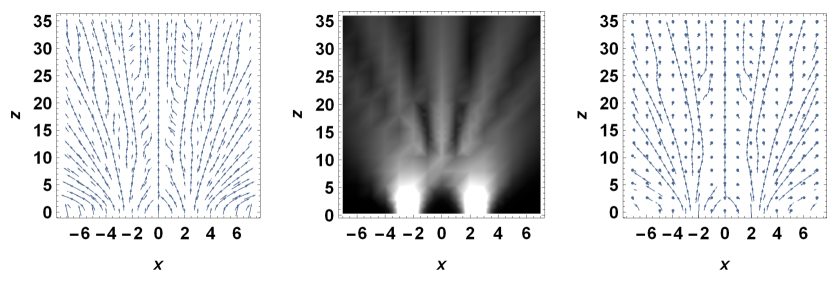
Figure 2: Bohmian trajectories in a Young setup with two Gaussian slits. Middle panel shows the probability density $\rho^{1/2}(x,z)$. Right panel contains the same trajectories as in the left panel, but weighted with $\rho^{1/2}$.

The middle panel of Fig. (2) shows $\rho^{1/2}$. The left panel shows the field $(v_{x},v_{z})$ and the right panel shows the weighted field $(\rho^{1/2}v_{x},\rho^{1/2}v_{z})$. This illustrates the effect of weighting with $\rho$ the integral curves of the field, thereby selecting from the infinity many ones (symbolically, those in the left panel) the cases actually realized in any experiment. We can only probabilistically assess which ones are these curves. They could be observed only as averaged trajectories, as it occurs when using weak-value measurements. The parameters used in Fig. (2) were chosen for illustrative purposes. Similar images have been obtained by Bliokh et al. bliokh with parameters taken from the experiments of Kocsis et al. kocsis2011 . Another option would be to proceed as Philippidis et al. did philippidis , using Feynman’s path integral method to get $\tilde{S}$, from which one can obtain BT.

Closing remarks

Finally, let us say that while this work leaves many questions still open, it has reached its goal of showing that WPD and BT can fit within a fully classical framework. The dynamical role assigned to EM vacuum should be accepted no more reluctantly than the analogous role of “space-time” in gravitation theory. If one is ready to accept that “space-time curvature” causes free particles to follow curvilinear trajectories, then one should also be ready to assign a similar role to EM vacuum. The latter has even more physical attributes, viz., $\epsilon_{0}$ and $\mu_{0}$, than the purely abstract concept that we call “space-time”. The second model we have presented is such, that any objection one could raise against it, would most likely also apply to classical electrodynamics. On the other hand, we stress that our approach, while being physically motivated, should be given a sound mathematical basis. The so-called “calculus of variations in the large” could be an appropriate tool. In any case, we can envision a wide, uncharted territory in classical physics, which remains open to be explored.

Supplemental Information

Carathéodory’s formulation

The usual approach in physics is to focus on a single curve $\mathcal{C}$ that renders the action $I$ extremal: $\delta I\equiv\delta\int L(x,\dot{x})ds=0$. However, as the calculus of variations shows bliss ; Caratheodory ; Rund , $\mathcal{C}$ exists only if it can be embedded in a whole field of extremals, also known as a Mayer field. The existence of such a field implies some integrability conditions. Carathéodory’s formulation Caratheodory makes clear how these integrability conditions relate to the Euler-Lagrange equations.

Let us summarize Carathéodory’s approach. We adopt a relativistic formulation just for the sake of generality. A non-relativistic formulation could be established along similar lines. Extremals satisfying $\delta\int L(x,\dot{x})ds=0$ are the same as those satisfying the so-called “equivalent variational problem” Caratheodory $\delta\int(L(x,\dot{x})-\dot{x}^{\mu}\partial_{\mu}S(x))ds=0$. Here, $S(x)$ is an auxiliary function. With its help, instead of seeking for a curve $\mathcal{C}$ that renders $I$ extremal, we seek for local extremal values. To this end, the Lagrangian is considered to be a function of $x$ and the velocity-field $v(x)$, i.e., $L=L(x,v(x))$. The extremal curve $\mathcal{C}$ is an integral curve of $v(x)$, i.e., it can be obtained by solving the first-order differential equations

$$\frac{dx^{\mu}(s)}{ds}=v^{\mu}(x(s)).$$ (37)

We thus seek for a velocity-field $v(x)$ whose integral curves render $\int Lds$ extremal. To this end, we impose the following condition:

$$L(x,v)-v^{\mu}(x)\partial_{\mu}S(x)=0,$$ (38)

and require that the expression on the left-hand side has zero as a stationary value with respect to variations of $v$. In the case of a maximum, for example, $L(x,w)-w^{\mu}\partial_{\mu}S<0$ for any field $w\neq v$. This guarantees that $\delta\int(L-\dot{x}^{\mu}\partial_{\mu}S)ds=0$, and so also $\delta\int L(x,\dot{x})ds=0$, because of the aforementioned equivalence of the two variational problems. Stationarity of the left-hand side of Eq. (38) with respect to $v$ leads to

$$\frac{\partial L(x,v)}{\partial v^{\mu}}=\frac{\partial S}{\partial x^{\mu}}.$$ (39)

Eqs. (38) and (39) are known as the fundamental equations of Carathéodory’s approach. On account of the integrability conditions $\partial^{2}S/\partial x^{\mu}\partial x^{\nu}=\partial^{2}S/\partial x^{\nu}\partial x^{\mu}$, it follows from Eq. (39) that

$$\frac{\partial}{\partial x^{\mu}}\left(\frac{\partial L(x,v(x))}{\partial v^{\nu}}\right)-\frac{\partial}{\partial x^{\nu}}\left(\frac{\partial L(x,v(x))}{\partial v^{\mu}}\right)=0.$$ (40)

From Eq. (40), we can get the equations of motion. Indeed, from Eq. (38) we obtain, by deriving with respect to $x^{\mu}$,

$$\frac{\partial L}{\partial x^{\mu}}+\frac{\partial L}{\partial v^{\sigma}}\frac{\partial v^{\sigma}}{\partial x^{\mu}}=\frac{\partial v^{\sigma}}{\partial x^{\mu}}\frac{\partial S}{\partial x^{\sigma}}+v^{\sigma}\frac{\partial^{2}S}{\partial x^{\mu}\partial x^{\sigma}}.$$ (41)

On using Eq. (39), Eq. (41) reduces to

$$\frac{\partial L}{\partial x^{\mu}}=v^{\sigma}\frac{\partial^{2}S}{\partial x^{\mu}\partial x^{\sigma}}.$$ (42)

Using $\partial^{2}S/\partial x^{\mu}\partial x^{\nu}=\partial^{2}S/\partial x^{\nu}\partial x^{\mu}$ first and then Eq. (39), we get

$$\frac{\partial^{2}S}{\partial x^{\mu}\partial x^{\sigma}}=\frac{\partial^{2}S}{\partial x^{\sigma}\partial x^{\mu}}=\frac{\partial^{2}L}{\partial x^{\sigma}\partial v^{\mu}}+\frac{\partial^{2}L}{\partial v^{\tau}\partial v^{\mu}}\frac{\partial v^{\tau}}{\partial x^{\sigma}},$$ (43)

so that Eq. (42) reads

$$\frac{\partial L}{\partial x^{\mu}}=v^{\sigma}\frac{\partial^{2}L}{\partial x^{\sigma}\partial v^{\mu}}+\frac{\partial^{2}L}{\partial v^{\tau}\partial v^{\mu}}\frac{\partial v^{\tau}}{\partial x^{\sigma}}v^{\sigma}.$$ (44)

If we now evaluate this last relation along a single extremal, $dx^{\mu}/ds=v^{\mu}(x(s))$, we obtain, after recognizing the right hand side of Eq. (44) as $d(\partial L/\partial v^{\mu})/ds$, the Euler-Lagrange equation:

$$\frac{d}{ds}\left(\frac{\partial L}{\partial\dot{x}^{\mu}}\right)-\frac{\partial L}{\partial x^{\mu}}=0.$$ (45)

Eq. (44) is therefore more general than Eq. (45), which follows from Eq. (44), but not the other way around.

Hamilton-Jacobi equation

The relativistic, free-particle Lagrangian reads

$$L=mc\left(\eta_{\mu\nu}v^{\mu}v^{\nu}\right)^{1/2}\equiv mc\,\phi.$$ (46)

From $\partial S/\partial x^{\mu}=\partial L/\partial v^{\mu}$ and Eq. (46) we get

$$v_{\mu}=\frac{\phi}{mc}\frac{\partial S}{\partial x^{\mu}}.$$ (47)

On replacing Eq. (47) in $\eta^{\mu\nu}v_{\mu}v_{\nu}=\phi^{2}$, we get the Hamilton-Jacobi equation

$$\eta^{\mu\nu}\left(\frac{\partial S}{\partial x^{\mu}}\right)\left(\frac{\partial S}{\partial x^{\nu}}\right)=m^{2}c^{2},$$ (48)

without having introduced a Hamiltonian, which in the homogeneous case is a rather laborious task Caratheodory ; Rund .

Invariance of Carathéodory’s fundamental equations under changes of the velocity field

As we said before, Carathéodory’s approach is based on two fundamental equations: (38) and (39). We deal with a relativistic, Lorentz invariant Lagrangian. Relativistic Lagrangians are homogeneous of the first degree in the velocities: $L(x,\lambda v)=\lambda L(x,v)$ (for $\lambda>0$). This property makes $\int L(x,\dot{x})ds$ invariant under parameter changes $s\rightarrow s^{\prime}$, a condition that must be met because $s$ has no physical meaning and can be arbitrarily chosen. We can then choose $s$ so that, say, $(\eta_{\mu\nu}\dot{x}^{\mu}\dot{x}^{\nu})^{1/2}=1$ along the sought-after extremal curve. We have a corresponding invariance when dealing with the velocity field $v^{\mu}(x)$. This time it is an invariance of the fundamental equations (38) and (39). Indeed, multiplication of Eq. (38) by a scalar function $\tilde{\phi}(x)>0$ leads to

$$\tilde{\phi}(x)\left(L(x,v)-v^{\mu}\partial_{\mu}S\right)=L(x,\tilde{\phi}v)-\left(\tilde{\phi}\,v^{\mu}\right)\partial_{\mu}S=L(x,\tilde{v})-\tilde{v}^{\mu}\partial_{\mu}S,$$ (49)

with $\tilde{v}:=\tilde{\phi}\,v$. From Eqs. (38) and (49), it follows that

$$L(x,\tilde{v})-\tilde{v}^{\mu}\partial_{\mu}S(x)=0,$$

which is Carathéodory’s first fundamental equation for $\tilde{v}$. Eq. (38) defines the Lagrangian of the “equivalent variational problem”:

$$L^{\ast}(x,v):=L(x,v)-v^{\mu}\partial_{\mu}S.$$

We see that

$$\frac{\partial L^{\ast}(x,\tilde{v})}{\partial v^{\mu}}=\frac{\partial L^{\ast}(x,\tilde{v})}{\partial\tilde{v}^{\nu}}\frac{\partial\tilde{v}^{\nu}}{\partial v^{\mu}}=\frac{\partial L^{\ast}(x,\tilde{v})}{\partial\tilde{v}^{\nu}}\left(\tilde{\phi}\,\delta^{\nu}_{\mu}\right)=\frac{\partial L^{\ast}(x,\tilde{v})}{\partial\tilde{v}^{\mu}}\,\tilde{\phi}.$$ (50)

On the other hand,

$$\frac{\partial L^{\ast}(x,\tilde{v})}{\partial v^{\mu}}=\frac{\partial}{\partial v^{\mu}}\left(\tilde{\phi}L^{\ast}(x,v)\right)=\tilde{\phi}\,\frac{\partial L^{\ast}(x,v)}{\partial v^{\mu}}=\tilde{\phi}\,\left(\frac{\partial L}{\partial v^{\mu}}-\frac{\partial S}{\partial x^{\mu}}\right)=0,$$ (51)

on account of Eq. (39). Equations (50) and (51) imply that $\partial L^{\ast}(x,\tilde{v})/\partial\tilde{v}^{\mu}=0$, i.e.,

$$\frac{\partial L(x,\tilde{v})}{\partial\tilde{v}^{\mu}}=\frac{\partial S(x)}{\partial x^{\mu}},$$ (52)

which is Carathéodory’s second fundamental equation for $\tilde{v}$. In summary, Eqs. (38) and (39) hold if we replace $v$ by $\tilde{v}$. In other words, both velocity fields $v$ and $\tilde{\phi}\,v$ solve our variational problem for the same $S(x)$. This allows us to choose $\tilde{\phi}$ conveniently, e.g., such that $(\tilde{v}_{\nu}\tilde{v}^{\nu})^{1/2}=1$.

Velocity field $v^{\nu}$ for a given $\pi^{\nu}$

As explained in the main text, given $\pi^{\nu}$, we can obtain $v^{\nu}$ from $n_{0}c\,v^{\nu}=(v_{\sigma}v^{\sigma})^{1/2}\pi^{\nu}$, with $\nu=0,\dots,3$. By squaring each of these four equations, we get

$$n_{0}^{2}c^{2}(v^{\nu})^{2}=\left[(v^{0})^{2}-\mathbf{v}^{2}\right](\pi^{\nu})^{2},\quad\nu=0,\dots,3.$$ (53)

Written in matrix form, this system of equations for the $(v^{\nu})^{2}$ reads

$$M\left((v^{0})^{2},(v^{1})^{2},(v^{2})^{2},(v^{3})^{2}\right)^{T}=0,$$ (54)

where $T$ stands for transpose and

$$M=\left(\begin{array}[]{cccc}n_{0}^{2}c^{2}-\pi_{0}^{2}&\pi_{0}^{2}&\pi_{0}^{2}&\pi_{0}^{2}\\ -\pi_{1}^{2}&n_{0}^{2}c^{2}+\pi_{1}^{2}&\pi_{1}^{2}&\pi_{1}^{2}\\ -\pi_{2}^{2}&\pi_{2}^{2}&n_{0}^{2}c^{2}+\pi_{2}^{2}&\pi_{2}^{2}\\ -\pi_{3}^{2}&\pi_{3}^{2}&\pi_{3}^{2}&n_{0}^{2}c^{2}+\pi_{3}^{2}\\ \end{array}\right).$$ (55)

For the system (54) to have a non-trivial solution, $\det M=0$. In our case,

$$\det M=(n_{0}c)^{6}[(n_{0}c)^{2}-\pi_{\nu}\pi^{\nu}].$$ (56)

Hence, with $\pi_{\nu}\pi^{\nu}=n_{0}^{2}c^{2}$, there are infinitely many solutions $(v^{\nu})^{2}$, in which one of the $v^{\nu}$ is a free parameter.

Two expressions for $\kappa$

In the main text, we derived the equation

$$\square\pi^{\mu}=\kappa\pi^{\mu},$$ (57)

from which it follows that $\pi_{\mu}\square\pi^{\mu}=\kappa\,\pi_{\mu}\pi^{\mu}$. By adding and subtracting $(\partial_{\sigma}\pi_{\mu})(\partial^{\sigma}\pi^{\mu})$ to $\pi_{\mu}\square\pi^{\mu}$, we obtain

$$(\partial_{\sigma}\pi_{\mu})(\partial^{\sigma}\pi^{\mu})+\pi_{\mu}\square\pi^{\mu}-(\partial_{\sigma}\pi_{\mu})(\partial^{\sigma}\pi^{\mu})=\partial_{\sigma}(\pi_{\mu}\partial^{\sigma}\pi{\mu})-(\partial_{\sigma}\pi_{\mu})(\partial^{\sigma}\pi^{\mu}).$$

Hence,

$$\partial_{\sigma}(\pi_{\mu}\partial^{\sigma}\pi^{\mu})-(\partial_{\sigma}\pi_{\mu})(\partial^{\sigma}\pi^{\mu})=\kappa\,\pi_{\mu}\pi^{\mu}.$$ (58)

Integrating over a volume $V$ with boundary $S$, using the divergence theorem and assuming von Neumann or Dirichlet boundary conditions, we obtain

$$\int_{V}\partial_{\sigma}(\pi_{\mu}\partial^{\sigma}\pi^{\mu})\,dV=\int_{S}(\pi_{\mu}\partial^{\sigma}\pi^{\mu})dS_{\sigma}=0.$$ (59)

Thus, integrating over $V$ both sides of Eq. (58), we get

$$\kappa=-\frac{\int_{V}(\partial_{\sigma}\pi_{\mu})(\partial^{\sigma}\pi^{\mu})dV}{\int_{V}\pi_{\mu}\pi^{\mu}dV}.$$ (60)

We now consider the tensor

$$K^{\alpha\beta}=\partial^{\alpha}\pi^{\beta}-\partial^{\beta}\pi^{\alpha}.$$ (61)

We see that

$$K_{\sigma\mu}K^{\sigma\mu}=(\partial_{\sigma}\pi_{\mu}-\partial_{\mu}\pi_{\sigma})(\partial^{\sigma}\pi^{\mu}-\partial^{\mu}\pi^{\sigma})=2\left[(\partial_{\sigma}\pi_{\mu})(\partial^{\sigma}\pi^{\mu})-(\partial_{\sigma}\pi_{\mu})(\partial^{\mu}\pi^{\sigma})\right].$$

Hence,

$$(\partial_{\sigma}\pi_{\mu})(\partial^{\sigma}\pi^{\mu})=\frac{1}{2}K_{\sigma\mu}K^{\sigma\mu}+(\partial_{\sigma}\pi_{\mu})(\partial^{\mu}\pi^{\sigma}).$$ (62)

On the other hand, using $\partial_{\sigma}\pi^{\sigma}=0$, we obtain

$$\partial_{\sigma}\left[\pi_{\mu}\partial^{\mu}\pi^{\sigma}\right]=(\partial_{\sigma}\pi_{\mu})(\partial^{\mu}\pi^{\sigma})+\pi_{\mu}\partial^{\mu}(\partial_{\sigma}\pi^{\sigma})=(\partial_{\sigma}\pi_{\mu})(\partial^{\mu}\pi^{\sigma}).$$ (63)

From Eqs. (62) and (63), we derive

$$\int_{V}(\partial_{\sigma}\pi_{\mu})(\partial^{\sigma}\pi^{\mu})dV=\frac{1}{2}\int_{V}K_{\sigma\mu}K^{\sigma\mu}dV+\int_{V}\partial_{\sigma}\left[\pi_{\mu}\partial^{\mu}\pi^{\sigma}\right]dV=\frac{1}{2}\int_{V}K_{\sigma\mu}K^{\sigma\mu}dV,$$ (64)

where we have used that $\int_{V}\partial_{\sigma}\left[\pi_{\mu}\partial^{\mu}\pi^{\sigma}\right]dV=\int_{S}\pi_{\mu}\partial^{\mu}\pi^{\sigma}dS_{\sigma}=0$. Eqs. (60) and (64) then lead to

$$\kappa=-\frac{1}{2}\frac{\int_{V}K_{\sigma\mu}K^{\sigma\mu}dV}{\int_{V}\pi_{\mu}\pi^{\mu}dV}.$$ (65)

Maxwell equations

In the main text, we considered the propagation equation

$$A^{\mu}(x)=\frac{4\pi}{c}\int G(x-x^{\prime})j_{(s)}^{\mu}(x^{\prime})d^{4}x^{\prime}.$$ (66)

From this equation, it follows that

$$\partial_{\mu}A^{\mu}(x) = \frac{4\pi}{c}\int\left(\partial_{\mu}G(x-x^{\prime})\right)j_{(s)}^{\mu}(x^{\prime})d^{4}x^{\prime}$$ (67)

$$= \frac{4\pi}{c}\int\left(-\partial_{\mu}^{\prime}G(x-x^{\prime})\right)j_{(s)}^{\mu}(x^{\prime})d^{4}x^{\prime}$$

$$= -\frac{4\pi}{c}\int\partial_{\mu}^{\prime}\left(G(x-x^{\prime})j_{(s)}^{\mu}(x^{\prime})\right)d^{4}x^{\prime}+\frac{4\pi}{c}\int G(x-x^{\prime})\left(\partial_{\mu}^{\prime}j_{(s)}^{\mu}(x^{\prime})\right)d^{4}x^{\prime}=0,$$

where in the last equality the first integral is shown to vanish by applying Gauss’ theorem and the boundary condition $j_{\mu}\rightarrow 0$ at infinity, and the second integral vanishes on account of charge conservation: $\partial_{\mu}j_{(s)}^{\mu}=0$.

We have then that, as a consequence of Eqs. (66) and (67),

$$\square A^{\nu}=\frac{4\pi}{c}j_{(s)}^{\nu},\quad\text{and}\quad\partial_{\nu}A^{\nu}=0.$$ (68)

From the above equations, it immediately follows that $F^{\mu\nu}=\partial^{\mu}A^{\nu}-\partial^{\nu}A^{\mu}$ satisfies the Maxwell equations

$$\partial_{\mu}F^{\mu\nu} = \frac{4\pi}{c}j_{(s)}^{\nu},$$ (69)

$$\partial_{\alpha}F_{\beta\gamma}+\partial_{\beta}F_{\gamma\alpha}+\partial_{\gamma}F_{\alpha\beta} = 0,$$ (70)

where (70) is an identity that follows from the definition of $F^{\mu\nu}$. Hence, the essential thrust of Maxwell equations lies on the propagation equation (66). Of course, (69) and (70) are gauge invariant whereas (66) is not. Classically, gauge invariance is relevant only in relation to the coupling of $A^{\mu}$ to some charge through a term of the form $(e/c)A_{\mu}v^{\mu}$ in the Lagrangian. As the charge’s equations of motion depend on $A^{\mu}$ only through $F^{\mu\nu}$, one may say that not $A^{\mu}$ itself but $F^{\mu\nu}$ is physically meaningful. It is easy to see that a gauge transformation $A^{\mu}\rightarrow\tilde{A}^{\mu}=A^{\mu}+\partial^{\mu}W$ amounts to a change $S\rightarrow\tilde{S}=S+(e/c)W$ in the auxiliary function used in Carathéodory’s fundamental equations (38) and (39). Thus, it does not matter that $A^{\mu}$ is in the Lorentz gauge. The only way to observe $A^{\mu}$ is by coupling it to a (test) charge, in order to register the latter’s response to it. This response is gauge invariant, according to (38) and (39), which imply the Euler-Lagrange equations.

References

- (1) S. Kocsis et al., Observing the Average Trajectories of Single Photons in a Two-Slit Interferometer, Science 332, 1170-1173 (2011).
- (2) D. H. Mahler et al., Experimental nonlocal and surreal Bohmian trajectories, Sci. Adv. 2, e1501466 (2016).
- (3) Y. Xiao, Y. Kedem, J.-S. Xu, C.-F. Li, G.-C. Guo, Experimental nonlocal and steering of Bohmian trajectories, Opt. Express 25, 14463-14472 (2017).
- (4) Y. Aharonov, D. Z. Albert, L. Vaidman, How the Result of a Measurement of a Component of the Spin of a Spin-1/2 Particle Can Turn Out to be 100. Phys. Rev. Lett. 60, 1351-1354 (1988).
- (5) C. Philippidis, C. Dewdney, B. J. Hiley, Quantum Interference and the Quantum Potential, Nuovo Cimento 52B, 15-28 (1979).
- (6) E. Cohen, M. Cortês, A. Elitzur, L. Smolin, Realism and causality. I. Pilot wave and retrocausal models as possible facilitators, Phys. Rev. D 102, 124027 (2020).
- (7) B.-G. Englert, M. O. Scully, G. Süssman, H. Walther, Surrealistic Bohm Trajectories, Z. Naturforsch. 47a, 117-1186 (1992).
- (8) M. O. Scully, Do Bohm trajectories always provide a trustworthy physical picture of particle motion?, Phys. Scripta, T76, 41-46, (1998).
- (9) C. Dewdney, L. Hardy, E. J. Squires, How late measurements of quantum trajectories can fool a detector, Phys. Lett. 184A, 6-11 (1993).
- (10) D. Dürr, W. Fusseder, S. Goldstein, N. Zanghi, Comment on “Surrealistic Bohm Trajectories”, Z. Naturforsch. 48a, 1261-1262 (1993).
- (11) B.-G. Englert, M. O. Scully, G. Süssman, H. Walther, Reply to Comment on ‘Surrealistic Bohm Trajectories’, Z. Naturforsch. 48a, 1263 (1993).
- (12) H. M. Wiseman, Grounding Bohmian mechanics in weak values and bayesianism, New J. Phys. 9, 165 (2007).
- (13) W. Schleich, M. Freyberger, M. S. Zubairy, Reconstruction of Bohm trajectories and wave functions from interferometric measurements, Phys. Rev. A 87, 014102 (2013).
- (14) J. Wu, B. B. Augstein, C. Figueira de Morisson Faria, Bohmian-trajectory analysis of high-order-harmonic generation: Ensemble averages, nonlocality, and quantitative aspects, Phys. Rev. A 88, 063416 (2013).
- (15) K. Y. Bliokh, A. Y. Bekshaev, A. G. Kofman, F. Nori, Photon trajectories, anomalous velocities and weak measurements: a classical interpretation, New J. Phys 15, 073022 (2013).
- (16) H. Z. Jooya, D. A. Telnov, S.-I. Chu, Exploration of the electron multiple recollision dynamics in intense laser fields with Bohmian trajectories, Phys. Rev. A 93, 063405 (2016).
- (17) G. Tastevin, F. Laloë, Surrealistic Bohmian trajectories do not occur with macroscopic pointers, Eur. Phys. J. D 72, 183 (2018).
- (18) S. Yu, X. Piao, N. Park, Bohmian photonics for indepent control of the phase and amplitude of waves, Phys. Rev. Lett. 120, 193902 (2018).
- (19) I. Cheng, Y. Ming, Z. J. Ding, Bohmian trajectory-bloch wave approach to dynamical simulation of electron diffraction in crystal, New J. Phys. 20, 113004 (2018).
- (20) N. Douguet, K. Bartschat, Dynamics of tunneling ionization using Bohmian mechanics, Phys. Rev. A 97, 013402 (2018).
- (21) Y. Xiao et al., Observing momentum disturbance in double-slit “which-way” measurements, Sci. Adv. 5 eaav9547 (2019).
- (22) P-C. Li, H.-C. Liu, H. Z. Jooya, C.-T. Belmiro Chu, S.-I. Chu, Resolving the quantum dynamics of near cut-off high-order harmonic generation in atoms by Bohmian trajectories, Opt. Express 29, 7134-7144 (2021).
- (23) R. P. Feynman, R. B. Leighton, M. Sands, The Feynman Lectures on Physics (Addison- Wesley, Reading MA, Vol. 1, Sec. 37-1, 1963).
- (24) N. D. Mermin, Hidden variables and the two theorems of John Bell, Rev. Mod. Phys. 65, 803-815 (1993).
- (25) K. von Meyenn (Hrsg.) Quantenmechanik und Weimarer Republik (Vieweg, Braunschweig; Wiesbaden, 1994).
- (26) F. Selleri, Paradossi e realtà. Saggio sui fondamenti della microfisica (Laterza, Roma-Bari, 1987).
- (27) Y. Aharonov et al., Finally making sense of the double-slit experiment, Proc. Natl. Acad. Sci. U.S.A. 114 6480-6485 (2017).
- (28) W. K. Wootters, W. H. Zurek, Complementarity in the double-slit experiment: Quantum nonseparability and a quantitative statement of Bohr’s principle, Phys. Rev. D 19, 473-484 (1979).
- (29) M. O. Scully, B.-G. Englert, H. Walther, Quantum optical tests of complementarity, Nature 351, 111-116 (1991).
- (30) G. Jaeger, A. Shimony, L. Vaidman, Two interferometric complementarities, Phys. Rev. A 51, 54-67 (1995).
- (31) B.-G. Englert, Fringe Visibility and Which-Way Information: An Inequality, Phys. Rev. Lett. 77, 2154-2157 (1996).
- (32) M. Jakob, J. A. Bergou, Quantitative complementarity relations in bipartite systems: Entanglement as a physical reality, Opt. Commun. 283, 827-830 (2010).
- (33) P. J. Coles, J. Kaniewski, S. Wehner, Equivalence of wave-particle duality to entropic uncertainty, Nat. Commun. 5, 5814 (2014).
- (34) X.-F. Qian, T. Malhotra, A. N. Vamivakas, J. H. Eberly, Coherence Constraints and the Last Hidden Optical Coherence, Phys. Rev. Lett. 117, 153901 (2016).
- (35) J. H. Eberly, X.-F. Qian, A. N. Vamivakas, Polarization-coherence theorem, Optica 4, 1113-1114 (2017).
- (36) X.-F. Qian, A. N. Vamivakas, J. H. Eberly, Entanglement limits duality and vice versa, Optica 5, 942-947 (2018).
- (37) A. Norrman, A. T. Friberg, G. Leuchs, Vector-light quantum complementarity and the degree of polarization, Optica 7, 93-97 (2020).
- (38) X.-F. Qian et al., Turning off quantum duality, Phys. Rev. Res. 2, 012016(R) (2020).
- (39) M. Miranda, M. Orszag, Controlling parameters of the wave-particle duality of a two-level atom in a double-slit scheme with cavity field, J. Opt. Soc. Am. B 38, 652-661 (2021).
- (40) T. Qureshi, Predictability, Distinguishability and Entanglement, Opt. Lett. 46, 492-495 (2021).
- (41) P. R. Holland, The quantum theory of motion (Cambridge University Press, Cambridge, 1993).
- (42) S. Haroche, Nobel Lecture: Controlling photons in a box and exploring the quantum classical boundary, Rev. Mod. Phys. 85, 1083-1102 (2013).
- (43) A. B. Nassar S. Miret-Artés, Dividing Line between Quantum and Classical Trajectories in a Measurement Problem: Bohmian Time Constant, Phys. Rev. Lett. 111, 150401 (2013).
- (44) D. Bohm, A Suggested Interpretation of the Quantum Theory in Terms of “Hidden” Variables. I, Phys. Rev. 85 166-179; A Suggested Interpretation of the Quantum Theory in Terms of "Hidden" Variables. II, ibid 85 180-193.
- (45) B. E. A. Saleh, M. C. Teich, Fundamentals of Photonics, John Wiley and Sons, Inc., 2nd. Ed., 2007.
- (46) E. Wolf, Introduction to the Theory of Coherence and Polarization of Light, Cambridge University Press, Cambridge, 2007.
- (47) C. Jönsson, Elektroneninterferenzen an mehreren künstlich hergestellten Feinspalten, Z. Phys. 161, 454-474 (1961).
- (48) G. A. Bliss, Lectures on the Calculus of Variations, The University of Chicago Press, Chicago, 1946.
- (49) C. Carathéodory, Calculus of Variations and Partial Differential Equations of the First Order, Holden-Day, Inc., San Francisco, 1967.
- (50) H. Rund,The Hamilton-Jacobi Theory in the Calculus of Variations, D. van Nostrand Comp., London, 1966.
- (51) See Supplemental Information.