SPIRAL: A superlinearly convergent incremental proximal algorithm for nonconvex finite sum minimization

Abstract

We introduce SPIRAL, a SuPerlinearly convergent Incremental pRoximal ALgorithm, for solving nonconvex regularized finite sum problems under a relative smoothness assumption. Each iteration of SPIRAL consists of an inner and an outer loop. It combines incremental gradient updates with a linesearch that has the remarkable property of never being triggered asymptotically, leading to superlinear convergence under mild assumptions at the limit point. Simulation results with L-BFGS directions on different convex, nonconvex, and non-Lipschitz differentiable problems show that our algorithm, as well as its adaptive variant, are competitive to the state of the art.

Keywords Finite sum minimization, nonsmooth nonconvex optimization, relative smoothness, superlinear convergence, KL inequality

Mathematics Subject Classification (2000) 90C06, 90C25, 90C26, 49J52, 49J53, 90C53

1 Introduction

We study nonconvex nonsmooth finite sum optimization problems of the form:

$$\textstyle\operatorname{minimize}_{z\in\mathbb{R}^{n}}\varphi(z)\coloneqq f(z)+g(z),\quad\text{where}\;f(z)\coloneqq\tfrac{1}{N}\textstyle\sum_{i=1}^{N}f_{i}(z).$$ (1.1)

The following basic assumptions are considered throughout the paper:

Assumption 1 (basic assumptions).

1. $f_{i}:\mathbb{R}^{n}\to\mathbb{R}$ is $L_{i}$-smooth relative to a distance-generating function $h_{i}:\mathbb{R}^{n}\to\mathbb{R}$ (cf. Definitions 2.3 and 2.1), $i\in[N]\coloneqq\{1,\dots,N\}$;

2. $g:\mathbb{R}^{n}\to\overline{\mathbb{R}}$ is proper and lower semicontinuous (lsc);

3. a solution exists: $\arg\min\varphi\neq\emptyset$.

The minimization problem (1.1) has gained considerable attention across various disciplines including machine learning (ML), signal and image processing, statistics, and control. Despite an upsurge in developing optimization methods to address such a problem, the potential of low-memory quasi-Newton methods has largely been neglected which can be partially attributed to the absence of theoretical foundations for handling nonsmooth settings. In the smooth strongly convex settings, competitive convergence rates compared to typical ML approaches have been documented in the ML community [47]. This work aims to address such large-scale problems in their full generality in the nonconvex, nonsmooth problem settings.

Stochastic gradient descent (SGD) is commonly employed for finite sum minimization problems. Despite it involving simple iterations, SGD requires a diminishing stepsize and, even in the strongly convex setting, can only achieve sublinear rates of convergence. These limitations have prompted the development of several stochastic and incremental methods such as SAG [61], SAGA [21], SDCA [62], SPIDER [28], SVRG [36] and its extensions [55, 29], SARAH [51], and zeroSARAH [41], which primarily target smooth functions ($g=0$) and are often restricted to the convex regime. To accommodate composite nonsmooth cost functions of the form (1.1), studies such as [14], proxSGD [31], proxSAGA and proxSVRG [56], proxSARAH [53], and SpiderBoost [70] have emerged recently.

The majority of the methods mentioned above incorporate a combination of stochastic and deterministic components in addressing the finite sum problem, aiming to diminish the variance of iterates toward the optimal point. Notably, algorithms such as SAGA, SVRG, and SARAH employ an outer loop to incorporate full gradients as the deterministic enhancement, along with an inner loop that incorporates stochastic gradients using randomized sampling with replacement. Furthermore, these algorithms adopt fixed stepsizes, in contrast to SGD which necessitates diminishing stepsizes to mitigate variance. In line with the spirit of these methods, the porposed algorithm also utilizes both inner and outer loops.

In its inner loop, the algorithm investigated in this study can be perceived as an incremental approach with a (shuffled) cyclic (randomized without replacement) sweeping rule. It should be mentioned that when combined with SGD, this sweeping rule demonstrates superior convergence and implementation efficiency [54, 5] compared to the randomized sweeping rule with replacement. Moreover, the analysis of SGD with (randomized) sampling without replacement has recently emerged in convex regimes, providing enhanced bounds compared to standard SGD [13, 16, 44, 32, 34]. Beyond SGD, the proposed algorithm, in its basic form without a linesearch, can be considered as a memory-efficient variant of Finito [22] and MISO [43]. It is worth noting that DIAG [46], proposed independently, studies the Finito/MISO algorithm under a cyclic sweeping rule and in the strongly convex case. More recently, [40] provided a comprehensive study of the above algorithms in the fully nonconvex setting. However, the above are all limited to first-order methods.

In its outer loop, one distinguishing characteristic of the proposed algorithm, which sets it apart from stochastic algorithms like SVRG and SARAH, is its utilization of quasi-Newton directions integrated with a linesearch while preserving the advantageous low-memory characteristic. In the context of this study, various methodologies have been explored to address nonconvex nonsmooth composite functions by employing quasi-Newton directions. For instance, methods presented in [68, 66, 1] have demonstrated the application of quasi-Newton directions to achieve superlinear convergence rates, albeit limited to scenarios involving a single smooth function within the composite cost. In the finite sum setting, approaches proposed by [47] and [60] have utilized quasi-Newton updates with global convergence guarantees and linear convergence rates. Furthermore, [74] has extended the utilization of quasi-Newton directions to decentralized learning scenarios.

To attain a superlinear convergence rate, the IQN method [45] has integrated quasi-Newton directions with incremental updates, albeit with only local convergence guarantees. Conversely, the approach introduced in [59] also exhibits a superlinear convergence rate but necessitates Hessian evaluation. It is noteworthy that the aforementioned algorithms are applicable in (strongly) convex cases. However, within the nonconvex nonsmooth setting, the algorithm proposed by [71] stands out with global convergence guarantees when the nonsmooth term is convex.

One of the restrictive aspects of the aforementioned works is that the cost functions are Lipschitz differentiable. However, in numerous practical applications, although the cost functions are differentiable, they fail to satisfy Lipschitz continuity assumptions on their gradients. This issue is exemplified in Section 5.2. To tackle such cost functions, the proposed algorithm goes beyond the classical notion of smoothness and employs the concept of relative smoothness, as introduced in [3, 42]. In connection with the proposed method, stochastic mirror descent (SMD) methods incorporate relative smoothness. Notable references in this area include [4, 48, 33, 19]. Within the convex setting, PLIAG [73] has been introduced as the Bregman variant of IAG [7, 8, 69]. Furthermore, [25] explores Bregman stochastic gradient descent (BSGD). In the nonconvex regime, [39] investigates a Bregman variant of Finito/MISO.

While the literature often assumes convexity for the nonsmooth term $g$, our proposed method, as indicated in Assumption 1, allows the nonconvex nature of this term. This enables the algorithm to effectively handle a wide range of nonconvex constraints, including rank constraints and $\ell_{0}$-norm ball constraints, as well as nonconvex regularizers such as $\ell^{p}$ with $p\in[0,1)$.

Motivated by the aforementioned advancements and recognizing the existing limitations in the literature, the proposed method addresses the optimization of regularized nonsmooth nonconvex cost functions, allowing the gradients of differentiable functions in the finite sum to be non-Lipschitz. To the best of our knowledge, none of the currently available methods in the literature that exhibit superlinear convergence rates have explicitly addressed the challenge of handling non-Lipschitz differentiable functions within nonsmooth nonconvex finite sum settings.

Contributions

The main contributions of the paper are as follows:

1. We propose SPIRAL with convergence guarantees for a wide class of finite sum problems. Not only are both the nonsmooth regularizer $g$ and the finite sum terms $f_{i}$ all allowed to be nonconvex, but also $f_{i}$ functions do not need to have Lipschitz-continuous gradients. Moreover, unlike Finito/MISO/DIAG, SPIRAL requires only $\mathcal{O}(n)$ memory allocation.

2. When the nonsmooth term is convex, we show that SPIRAL converges superlinearly when the employed quasi-Newton directions are superlinear (cf. Definition 4.11) and the linesearch will eventually never be invoked (cf. Theorem 4.12) under mild assumptions. This is also supported by our simulation results. Moreover, global (as opposed to local) convergence is guaranteed regardless of any assumptions placed on the quasi-Newton directions or the convexity of the nonsmooth term (cf. Theorem 4.7).

3. Finally, an adaptive variant employing appropriate backtracking linesearch is introduced that adapts to the local relative smoothness moduli of $f_{i}$ while maintaining convergence guarantees and the $\mathcal{O}(n)$ memory requirement.

2 Preliminaries

2.1 Notation

In this section, we provide basic notations. The interested reader may refer to [58, 57] for details. The set of natural numbers is denoted by $\mathbb{N}=\{0,1,2,\ldots\}$. The set of real and extended-real numbers are $\mathbb{R}\coloneqq(-\infty,\infty)$ and $\overline{\mathbb{R}}\coloneqq\mathbb{R}\cup\{\infty\}$, and the set of positive reals is denoted by $\mathbb{R}_{+}\coloneqq[0,\infty)$. We also use the notation $[N]\coloneqq\{1,2,\cdots,N\}$. We denote by $\langle{}\cdot{},{}\cdot{}\rangle$ and $\|{}\cdot{}\|$ the standard Euclidean inner product and the induced norm. The distance of a point $x\in\mathbb{R}^{n}$ to a nonempty set $S\subseteq\mathbb{R}^{n}$ is given by $\operatorname{dist}(x,S)=\inf_{z\in S}{\|z-x\|}$. For a vector $\bm{w}=(w_{1},\ldots,w_{r})\in\mathbb{R}^{\sum_{i}n_{i}}$, $w_{i}\in\mathbb{R}^{n_{i}}$ is used to denote its $i$-th block coordinate. The identity operator is denoted by $\operatorname{id}$.

For a sequence $(x^{k})_{k\in\mathbb{N}}$ we write $(x^{k})_{k\in\mathbb{N}}\subseteq E$ to indicate that $x^{k}\in E$ for all $k\in\mathbb{N}$. We use the following notions of convergence rate: a sequence $(x^{k})_{k\in\mathbb{N}}$ is said to converge to a point $x^{\star}$:

• (at least) $Q$-linearly (with quotient rate) with $Q$-factor given by $\sigma\in(0,1)$, if there exists $k_{0}\in\mathbb{N}$ such that for all $k\geq k_{0}$,

  $$\|x^{k+1}-x^{\star}\|\leq\sigma\|x^{k}-x^{\star}\|.$$

• (at least) R-linearly (with root rate) if there exists a sequence of nonnegative scalars $({v^{k}})_{k\in\mathbb{N}}$ such that $\|x^{k}-x^{\star}\|\leq v^{k}$ and $(v^{k})_{k\in\mathbb{N}}$ converges Q-linearly to zero.

• superlinearly if either $x^{k}=x^{\star}$ for some $k\in\mathbb{N}$ or

  $$\lim_{k\to\infty}\frac{\|x^{k+1}-x^{\star}\|}{\|x^{k}-x^{\star}\|}=0.$$

We use the notation $Q:\mathbb{R}^{n}\rightrightarrows\mathbb{R}^{m}$ to indicate a mapping from each point $x\in\mathbb{R}^{n}$ to a subset $Q(x)$ of $\mathbb{R}^{m}$. The graph of $Q$ is the set $\operatorname{gph}Q\coloneqq\{(x,y)\in\mathbb{R}^{n}\times\mathbb{R}^{m}:y\in Q(x)\}$, and the set of its fixed points is defined as $\operatorname{fix}Q\coloneqq\{x\in\mathbb{R}^{n}:x\in Q(x)\}$. We say that $Q$ is outer semicontinuous (osc) if $\operatorname{gph}Q$ is a closed subset of $\mathbb{R}^{n}\times\mathbb{R}^{m}$, and locally bounded if for every bounded $U\subset\mathbb{R}^{n}$ the set $\bigcup_{x\in U}Q(x)$ is bounded.

The domain of an extended-real-valued function $\phi:\mathbb{R}^{n}\to\overline{\mathbb{R}}$ is the set $\operatorname{dom}\phi\coloneqq\{x\in\mathbb{R}^{n}:\phi(x)<\infty\}$ and $\operatorname{epi}\phi\coloneqq\{(x,\alpha)\in\mathbb{R}^{n}\times\mathbb{R}:\phi(x)\leq\alpha\}$ is its epigraph set. Function $\phi$ is said to be proper if $\operatorname{dom}\phi\neq\emptyset$, and lower semicontinuous (lsc) if $\operatorname{epi}\phi$ is a closed subset of $\mathbb{R}^{n+1}$. We say that $\phi$ is level bounded if its $\alpha$-sublevel set $\operatorname{lev}_{\leq\alpha}\phi\coloneqq\{x\in\mathbb{R}^{n}:\phi(x)\leq\alpha\}$ is bounded for all $\alpha\in\mathbb{R}$. The indicator function $\delta_{X}$ of a nonempty set $X\subseteq\mathbb{R}^{n}$ is defined by

$$\delta_{X}(x)\coloneqq\begin{cases}0&\ \ \ \ \textrm{if}\;\,x\in X\\ +\infty&\ \ \ \ \textrm{if}\;\,x\notin X.\end{cases}$$ (2.1)

The indicator function $\delta_{X}$ is closed if and only if $X$ is a closed set.

We denote by $\hat{\partial}\phi:\mathbb{R}^{n}\rightrightarrows\mathbb{R}^{n}$ the regular sub-differential of $\phi$, where

$$v\in\hat{\partial}\phi(\bar{x})\iff\liminf_{\bar{x}\neq x\to\bar{x}}{\frac{\phi(x)-\phi(\bar{x})-\langle v,x-\bar{x}\rangle}{\|x-\bar{x}\|}}\geq 0.$$

The regular sub-differential is closed- and convex-valued. The (limiting) sub-differential of $\phi$ is $\partial\phi:\mathbb{R}^{n}\rightrightarrows\mathbb{R}^{n}$, where $v\in\partial\phi(x)$ iff $x\in\operatorname{dom}\phi$ and there exists a sequence $(x^{k},v^{k})_{k\in\mathbb{N}}\subseteq\operatorname{gph}\hat{\partial}\phi$ such that $(x^{k},\phi(x^{k}),v^{k})\to(x,\phi(x),v)$ as $k\to\infty$.

A necessary condition for local minimality of $x$ for $\phi$ is $0\in\hat{\partial}\phi(x)$, see [57, Thm. 10.1]. Finally, the set of $r$ times continuously differentiable functions over $\mathbb{R}^{n}$ is denoted by $\mathcal{C}^{r}=\mathcal{C}^{r}(\mathbb{R}^{n})$.

2.2 Relative smoothness

We start by formally defining the notion of distance generating function, Bregman distance, and relative smoothness [3, 42, 65].

Definition 2.1 (Distance-generating function (dgf)).

A strictly convex function $h:\mathbb{R}^{n}\to\mathbb{R}$ that is continuously differentiable everywhere will be referred to as a distance-generating function (dgf).

While some results here can be presented with $\operatorname{dom}h\subset\mathbb{R}^{n}$, for the sake of simplicity and global convergence analysis, we continue with $\operatorname{dom}h=\mathbb{R}^{n}$. The Bregman distance associated with a dgf is defined as:

Definition 2.2 (Bregman distance).

Given a dgf $h:\mathbb{R}^{n}\to\mathbb{R}$, the Bregman distance $\operatorname{D}_{h}:\mathbb{R}^{n}\times\mathbb{R}^{n}\to\mathbb{R}_{+}$ is defined as,

$$\operatorname{D}_{h}(y,x)\coloneqq h(y)-h(x)-\langle\nabla h(x),y-x\rangle\quad\text{for all }x,y\in\mathbb{R}^{n}.$$ (2.2)

Definition 2.3 (Relative smoothness [12, Def. 2.2]).

A function $f:\mathbb{R}^{n}\to\mathbb{R}$ is smooth relative to a dgf $h:\mathbb{R}^{n}\to\mathbb{R}$ if there exists $L\geq 0$ such that $Lh\pm f$ are convex functions on $\mathbb{R}^{n}$. In this case, we say that $f$ is $L$-smooth (relative to $h$) to make the modulus $L$ explict.

Fact 2.4 (Descent lemma [12, Lem. 2.1]).

If $f:\mathbb{R}^{n}\to\mathbb{R}$ is $L$-smooth relative to a dgf $h:\mathbb{R}^{n}\to\mathbb{R}$, then for all $x,y\in\mathbb{R}^{n}$

$$|f(y)-f(x)-\langle\nabla f(x),y-x\rangle|\leq L\operatorname{D}_{h}(y,x).$$

Note that in the Euclidean case, the dgf and the corresponding Bregman distance reduce to $h=\tfrac{1}{2}\|\cdot\|^{2}$ and $\operatorname{D}_{h}(y,x)=\tfrac{1}{2}\|y-x\|^{2}$, respectively, and 2.4 reduces to the ordinary descent lemma [6, Prop. A.24] for smooth functions.

Relative to a dgf $h:\mathbb{R}^{n}\to\mathbb{R}$, the (left) Bregman proximal mapping of a proper lsc function $\phi:\mathbb{R}^{n}\to\overline{\mathbb{R}}$ is the set-valued mapping $\operatorname{prox}_{\phi}^{h}:\mathbb{R}^{n}\rightrightarrows\mathbb{R}^{n}$ defined as [37, Def. 2.2]

$$\operatorname{prox}_{\phi}^{h}(x)\coloneqq{} \operatorname{argmin}_{w\in\mathbb{R}^{n}}\bigl{\{}\phi(w)+\operatorname{D}_{h}(w,x)\bigr{\}},$$ (2.3)

and its value function is the Bregman Moreau envelope $$\phi^{h}:\mathbb{R}^{n}\to\mathbb{R}$$

$$\phi^{h}(x)\coloneqq{} \min_{w\in\mathbb{R}^{n}}\bigl{\{}\phi(w)+\operatorname{D}_{h}(w,x)\bigr{\}}.$$ (2.4)

Moreover it is evident from (2.3) and Definition 2.2 that if $v\in\operatorname{prox}_{\phi}^{h}(x)$, then

$$\nabla h(x)-\nabla h(v)\in\hat{\partial}\phi(v),$$ (2.5)

and the converse also holds when $\phi$ is convex. Whenever the superscript $h$ is omitted from $\operatorname{prox}_{\phi}^{h}$, it refers to the Euclidean proximal mapping with $h=\tfrac{1}{2}\|\cdot\|^{2}$.

3 Proposed algorithm

Algorithm 1 SPIRAL

1.1:18:

$z^{\rm init}\in\mathbb{R}^{n}$,  $\gamma_{i}\in(0,\nicefrac{{N}}{{L_{i}}})$, $\forall i\in[N]$,  $s^{\rm 0}=\sum_{i=1}^{N}{\frac{1}{\gamma_{i}}\nabla h_{i}(z^{\rm init})-\frac{1}{N}\nabla f_{i}(z^{\rm init})}$,

maximum number of backtracks $q_{\rm max}\in\mathbb{N}\cup\{\infty\}$ (e.g. $q_{\rm max}=2$),  $\beta\in(0,1)$

1.2:18:

1.3:18: $z^{k}\in\operatorname{t}(s^{k})$

1.4:18: $\bar{s}^{k}=\sum_{i=1}^{N}{\frac{1}{\gamma_{i}}\nabla h_{i}(z^{k})-\frac{1}{N}\nabla f_{i}(z^{k})}$ (full update)

1.5:18: $v^{k}\in\operatorname{t}(\bar{s}^{k})$

1.6:18:choose $d^{k}\in\mathbb{R}^{n}$ at $z^{k}$ (e.g. based on a quasi-Newton method for solving $\operatorname{r}_{\hat{h}}(z)=0$)

1.7:18:set $\tau_{k}=1,q_{k}=0$ (linesearch) a: $u^{k}=\tau_{k}z^{k}+(1-\tau_{k})v^{k}+\tau_{k}{d^{k}}$ b: $\tilde{s}^{k}=\sum_{i=1}^{N}{\frac{1}{\gamma_{i}}\nabla h_{i}(u^{k})-\frac{1}{N}\nabla f_{i}(u^{k})}$ (full update) c: $y^{k}\in\operatorname{t}(\tilde{s}^{k})$ d: if $\mathcal{L}(y^{k},u^{k})\leq\mathcal{L}(v^{k},z^{k})$ go to step 1.8 e: else if $q_{k}=q_{\max}$ then $u^{k}=v^{k}$,  $\tilde{s}^{k}=\sum_{i=1}^{N}{\frac{1}{\gamma_{i}}\nabla h_{i}(u^{k})-\frac{1}{N}\nabla f_{i}(u^{k})}$, and go to step 1.8 f: else $\tau_{k}\leftarrow\beta\tau_{k}$,  $q_{k}\leftarrow q_{k}+1$, and go to step alg:1:ls.a

1.8:18:$s^{k}\leftarrow\tilde{s}^{k}$

1.9:18:for $\ell=1,\ldots,N$ do(incremental loop)

1.10:18:     randomly choose $i^{\ell}\in[N]$ without replacement

1.11:18:     $\tilde{z}_{i^{\ell}}^{k}\in\operatorname{t}(s^{k})$

1.12:18:     $s^{k}\leftarrow s^{k}+\left[\frac{1}{\gamma_{i^{\ell}}}\nabla h_{i^{\ell}}(\tilde{z}^{k}_{i^{\ell}})-\frac{1}{N}\nabla f_{i^{\ell}}(\tilde{z}^{k}_{i^{\ell}})-\frac{1}{\gamma_{i^{\ell}}}\nabla h_{i^{\ell}}(u^{k})+\frac{1}{N}\nabla f_{i^{\ell}}(u^{k})\right]$

1.13:18:$s^{k+1}\leftarrow s^{k}$

1.14:18:

The proposed method, SPIRAL, is outlined in Algorithm 1 to address the optimization problem (1.1). SPIRAL employs the set-valued mapping $\operatorname{t}:\mathbb{R}^{n}\rightrightarrows\mathbb{R}^{n}$ as its major oracle, defined as

$$\textstyle\operatorname{t}(s)\coloneqq\operatorname{argmin}_{w\in\mathbb{R}^{n}}\left\{g(w)+\sum_{i=1}^{N}\tfrac{1}{\gamma_{i}}h_{i}(w)-\langle s,w\rangle\right\},$$ (3.1)

where $h_{i}$ is the dgf corresponding to function $f_{i}$ as in ass:basic.A1. Within both the outer and inner loops, the mapping $\operatorname{t}$, utilized in steps 1.3, 1.5, alg:1:ls.c, and 1.11, represents the proximal steps. It is important to note that in the case of Euclidean space, where the functions $f_{i}$ are $L_{i}$-smooth relative to $h_{i}=\frac{1}{2}\|\cdot\|^{2}$, the oracle $\operatorname{t}$ reduces to the Euclidean proximal mapping with updates of the form $z^{k}\in\operatorname{prox}_{\hat{\gamma}g}(\hat{\gamma}s^{k})$, where $\hat{\gamma}^{-1}=\sum_{i=1}^{N}\gamma_{i}^{-1}$. Similarly, the iterates $v^{k}$, $y^{k}$, and $\tilde{z}^{k}_{i}$ are updated using the same $\operatorname{prox}_{\hat{\gamma}g}$ function. A detailed description of the Euclidean version of the algorithm can be found in Appendix E.2.

SPIRAL employs the function $\mathcal{L}:\mathbb{R}^{n}\times\mathbb{R}^{n}\to\mathbb{R}$ defined by

$$\mathcal{L}(y,x)\coloneqq\varphi(y)+\operatorname{D}_{\hat{h}}(y,x)\quad\text{with}\;\,y\in\operatorname{t}(\nabla\hat{h}(x))$$ (3.2)

in its linesearch, where $\hat{h}_{i}:\mathbb{R}^{n}\to\mathbb{R}$ and $\hat{h}:\mathbb{R}^{n}\to\mathbb{R}$ are

$$\textstyle\hat{h}_{i}\coloneqq\frac{1}{\gamma_{i}}h_{i}-\frac{1}{N}f_{i},\quad\hat{h}\coloneqq\sum_{i=1}^{N}\hat{h}_{i}.$$ (3.3)

The function $\mathcal{L}$ is considered as a suitable Lyapunov function in our convergence analysis. The linesearch in step 1.7 interpolates the iterate $u^{k}$ between the candidate fast update $z^{k}+d^{k}$, corresponding to $\tau_{k}=1$, and the safeguard step $v^{k}$ which is approached as $\tau_{k}\searrow 0$. The iterate $u^{k}$ is selected whenever it is a descent direction for the Lyapunov function $\mathcal{L}$ (cf. Remark 4.5 regarding the well definedness of the linesearch).

One distinguishing characteristic of SPIRAL, which sets it apart from stochastic algorithms such as SVRG and SARAH, is its utilization of directions $d^{k}$ in step 1.6 based on second-order-like information of the set-valued residual mapping $\operatorname{r}_{\hat{h}}:\mathbb{R}^{n}\rightrightarrows\mathbb{R}^{n}$ defined as

$$\operatorname{r}_{\hat{h}}\coloneqq\operatorname{id}-\operatorname{t}\circ\nabla\hat{h}.$$ (3.4)

This feature allows SPIRAL to achieve a superlinear convergence rate, given certain mild conditions (cf. Theorem 4.12). Given that the inclusion $0\in\operatorname{r}_{\hat{h}}(z^{\star})$ holds at a stationary point $z^{\star}$ (as discussed in Section 4.1 and expressed in (4.7)), the direction $d^{k}$ is determined based on solving this inclusion. Semismooth Newton directions [66] can be utilized to compute $d^{k}$; however, this approach relies on access to second-order oracle information. As an alternative to circumvent this requirement, quasi-Newton methods can be employed to compute the directions $d^{k}$. Specifically, we employ the update rule

$$d^{k}=-H^{k}\operatorname{r}_{\hat{h}}(z^{k})$$ (3.5)

where $H^{k}$ represents a linear operator that approximates the second-order information of the residual mapping $\operatorname{r}_{\hat{h}}$. It is worth noting that although $\operatorname{r}_{\hat{h}}$ is a set-valued mapping, it typically exhibits single-valuedness and other desirable properties in the vicinity of stationary points of the objective function $\varphi$ (see e.g. [1, Thm. 3.10 and 3.11]). Consequently, the updates for $H^{k}$ can be implemented using popular quasi-Newton methods such as Broyden’s method, BFGS, and L-BFGS (cf. Section 4.4 for further discussion).

SPIRAL can accommodate various sweeping rules depending on the memory requirements. The following remark comments on two different settings.

Remark 3.1 (sweeping rule in the incremental loop).

1. low-memory setting: in this setting, SPIRAL employs a (shuffled) cyclic (randomized without replacement) sweeping rule within the incremental loop, and unlike Finito/MISO/DIAG methods, it does not require storing individual function gradients $\nabla f_{i}$. Instead, SPIRAL only requires storing the finite sum of gradients as $\nabla\hat{h}$, using the vectors $s^{k}$, $\tilde{s}^{k}$, and $\bar{s}^{k}$. Additionally, in the incremental loop, updating this sum in the vector $s^{k}$ is carried out in a memory-efficient manner since the vector $u^{k}$ is known and fixed due to choosing $i^{\ell}$ without replacement. This advantageous characteristic allows SPIRAL to require only $\mathcal{O}(n)$ memory allocation, making it suitable for large-scale optimization problems.

2. high-memory setting: in this setting, by utilizing a memory of $\mathcal{O}(nN)$ and saving $\tilde{z}^{k}_{j}$ for all $j\in[N]$, like Finito/MISO/DIAG, the incremental loop can be replaced by a randomized loop of an arbitrary depth.

Computational complexity. The overall computational complexity, measured in terms of gradient evaluations per iteration, is $\mathcal{O}\big{(}(4+\kappa)N\big{)}$. This includes $2+\kappa$ full gradient evaluations performed outside of the inner loop, where $\kappa$ represents the number of backtracks in the linesearch, and two gradient evaluations performed in each iteration of the inner loop. It is worth noting that in certain problems like least squares, nonnegative principal component analysis, and logistic regression, the gradients can be obtained by storing the inner product between data points and the evaluated points. Consequently, the gradient evaluations $\nabla\hat{h}_{i}(u^{k})$ in step 1.12 can be derived from the computations in step alg:1:ls.b, thereby reducing the computational complexity to $\mathcal{O}\big{(}(3+\kappa)N\big{)}$. In addition, based on numerical experiments, it is beneficial to limit the number of backtracks using a maximum value $q_{\max}$. It is important to note that, as demonstrated in Theorem 4.12, under mild conditions, the unit stepsize $\tau_{k}=1$ is eventually always accepted ($\kappa=0$), allowing for pure quasi-Newton type updates in step alg:1:ls.a and avoiding any further backtracks and computation.

4 Convergence Analysis

In the subsequent subsections, we study the convergence of SPIRAL by reformulating the problem (1.1) in the lifted space. We will thus recast the Lyapunov function $\mathcal{L}$ in (3.2) into this new space and study it along the iterates generated by SPIRAL. In the lifted space, we can show that block coordinate updates in the incremental loop result in sufficient descent for the Lyapunov function, while this is not necessarily the case for the objective function. Utilizing newly reformulated operators, we then outline Algorithm 1 in the lifted space. Having new insight into the mechanism of SPIRAL, in Sections 4.3 to 4.5 we establish its convergence in various regimes.

4.1 Problem Reformulation

We recast (1.1) as the following lifted consensus optimization problem:

$$\operatorname{minimize}_{\bm{z}=(z_{1},\dots,z_{N})\in\mathbb{R}^{Nn}}\Phi(\bm{z})\coloneqq{} \underbracket{\frac{1}{N}\sum_{i=1}^{N}f_{i}(z_{i})}_{\coloneqq F(\bm{z})}+\underbracket{\frac{1}{N}\sum_{i=1}^{N}g(z_{i})+\delta_{\Delta}(\bm{z})}_{\coloneqq G(\bm{z})}$$ (4.1)

$$\text{where}\quad\Delta\coloneqq{} \left\{\bm{z}=(z_{1},\dots,z_{N})\in\mathbb{R}^{Nn}|z_{1}=\dots=z_{N}\right\}$$

is the consensus set. Note that $\Phi(\bm{z})=\varphi(z)$ whenever $\bm{z}=(z,\dots,z)\in\Delta$. Define

$$\mathcal{M}_{\hat{H}}(\bm{w},\bm{z})\coloneqq\Phi(\bm{w})+\operatorname{D}_{\hat{H}}(\bm{w},\bm{z}),\quad\text{with }\;\hat{H}(\bm{x})\coloneqq\sum_{i=1}^{N}\hat{h}_{i}(x_{i}),$$ (4.2)

for any $(\bm{w},\bm{z})\in\mathbb{R}^{Nn}\times\mathbb{R}^{Nn}$, where $\hat{h}_{i}$ is defined in (3.3). The model $\mathcal{M}_{\hat{H}}$ is in particular a majorizing model of $\Phi$, in that from (3.3), and Definitions 2.1 and 2.3, it is evident that whenever $\gamma_{i}\in(0,\nicefrac{{N}}{{L}}_{i})$, $\hat{h}_{i}$ and consequently $\hat{H}$ are dgfs, hence $\operatorname{D}_{\hat{H}}(\bm{w},\bm{z})\geq 0$ for all $\bm{w},\bm{z}\in\mathbb{R}^{Nn}$ and

1. $\mathcal{M}_{\hat{H}}(\bm{w},\bm{z})\geq\Phi(\bm{w})$ for all $\bm{w},\bm{z}\in\mathbb{R}^{Nn}$;

2. $\mathcal{M}_{\hat{H}}(\bm{z},\bm{z})=\Phi(\bm{z})$ for all $\bm{z}\in\mathbb{R}^{Nn}$.

The Bregman proximal mapping $\operatorname{prox}_{\Phi}^{\hat{H}}:\mathbb{R}^{Nn}\rightrightarrows\mathbb{R}^{Nn}$ and its value function the Bregman Moreau envelope $\Phi^{\hat{H}}:\mathbb{R}^{nN}\to\mathbb{R}$ (recall the definitions in (2.3)) are then defined as

$$\operatorname{prox}_{\Phi}^{\hat{H}}(\bm{z})\coloneqq\operatorname{argmin}_{\bm{w}\in\mathbb{R}^{Nn}}\mathcal{M}_{\hat{H}}(\bm{w},\bm{z}),\quad\Phi^{\hat{H}}(\bm{z})\coloneqq\min_{\bm{w}\in\mathbb{R}^{Nn}}\mathcal{M}_{\hat{H}}(\bm{w},\bm{z}).$$ (4.3)

The corresponding forward-backward residual is defined as $\operatorname{R}_{\hat{H}}=\operatorname{id}-\operatorname{prox}_{\Phi}^{\hat{H}}$. The envelope $\Phi^{\hat{H}}$ is considered as the Lyapunov function in our convergence studies.

We proceed with the following fact that is the key to our convergence analysis. First, to facilitate our subsequent analysis, we introduce the matrix $U_{i}\in\mathbb{R}^{Nn\times n}$ whose $i$-th block rows form an identity matrix. For a given vector $y\in\mathbb{R}^{n}$, the action of $U_{i}$ can be expressed as:

$$U_{i}y={(0,\dots,0,\!\overbracket{\,y\,}^{\mathclap{i\text{-th block}}}\!,0,\dots,0)}.$$ (4.4)

The following fact demonstrates that block-coordinate updates result in descent on the Bregman Moreau envelope $\Phi^{\hat{H}}$ in (4.3). As remarked above this is not necessarily the case for the cost function.

Fact 4.1 (Descent lemma [39, Lem. 4.2]).

Suppose that Assumption 1 holds, and let $\bm{x}=(x_{1},\dots,x_{N})$. Fix $\bm{y}\in\operatorname{prox}_{\Phi}^{\hat{H}}(\bm{x})$, and let $\mathcal{I}\subseteq[N]$ be a subset of indices. Consider the block-coordinate update

$$\textstyle\bm{v}=\bm{x}+\sum_{i\in\mathcal{I}}U_{i}U_{i}^{\top}(\bm{y}-\bm{x}),$$ (4.5)

where $U_{i}$ is as defined in (4.4). Then,

$$\Phi^{\hat{H}}(\bm{v})\leq\Phi^{\hat{H}}(\bm{x})-\operatorname{D}_{\hat{H}}(\bm{v},\bm{x}).$$ (4.6)

This observation is then utilized to establish that the limit points of the sequence $(z^{k})_{k\in\mathbb{N}}$ correspond to stationary points of the function $\varphi$, which, in the nonconvex setting, represents the necessary condition $0\in\hat{\partial}\varphi(z^{\star})$.

In the following fact we present some of useful properties of the Bregman proximal mapping $\operatorname{prox}_{\Phi}^{\hat{H}}$ and the Bregman distance $\operatorname{D}_{\hat{H}}$, and expand on their relation to those defined in Section 3.

Fact 4.2 (Bregman proximal mapping [39, Lem. 3.1]).

Suppose that Assumption 1 holds and let $\gamma_{i}\in(0,\tfrac{N}{L_{i}})$. Then, the following hold:

1. $\operatorname{D}_{\hat{H}}(\bm{v},\bm{z})\geq\sum_{i=1}^{N}(\tfrac{1}{\gamma_{i}}-\tfrac{L_{f_{i}}}{N})\operatorname{D}_{h_{i}}(v_{i},z_{i})$, for $(\bm{v},\bm{z})\in\mathbb{R}^{Nn}\times\mathbb{R}^{Nn}$.

2. $\operatorname{prox}_{\Phi}^{\hat{H}}(\bm{z})=\{(v,\cdots,v):v\in\operatorname{t}(\sum_{i=1}^{N}\nabla\hat{h}_{i}(z_{i}))\}$, where $\operatorname{t}$ is as in (3.1), is a nonempty and compact subset of $\Delta$.

When $\bm{z}\in\Delta$, one has a lower-dimensional representation of the Bregman Moreau envelope $\Phi^{\hat{H}}$, provided in the following corollary of 4.2.

Corollary 4.3 (lower-dimensional representations).

Let Assumption 1 hold and let $\gamma_{i}\in(0,\tfrac{N}{L_{i}})$. Then, with the Bregman Moreau operator and the envelope associated with $\varphi$ in (1.1) given by

$$\operatorname{t}_{\hat{h}}(z)={} \operatorname{argmin}_{w\in\mathbb{R}^{n}}\left\{\varphi(w)+\operatorname{D}_{\hat{h}}(w,z)\right\},$$

$$\varphi^{\hat{h}}(z)={} \min_{w\in\mathbb{R}^{n}}\left\{\varphi(w)+\operatorname{D}_{\hat{h}}(w,z)\right\}=\mathcal{L}(v,z),\;\text{with}\;v\in\operatorname{t}_{\hat{h}}(z),$$

it holds that $\operatorname{t}_{\hat{h}}=\operatorname{t}\circ\nabla\hat{h}=\operatorname{prox}_{\varphi}^{\hat{h}}$, and $\Phi^{\hat{H}}(\bm{z})=\varphi^{\hat{h}}(z)$ for $\bm{z}=(z,\ldots,z)\in\Delta$. Moreover,

1. $\operatorname{D}_{\hat{h}}(v,z)\geq\sum_{i=1}^{N}(\tfrac{1}{\gamma_{i}}-\tfrac{L_{f_{i}}}{N})\operatorname{D}_{h_{i}}(v,z)$, for $(v,z)\in\mathbb{R}^{n}\times\mathbb{R}^{n}$.

2. If $v\in\operatorname{prox}_{\varphi}^{\hat{h}}(z)$, then $\nabla\hat{h}(z)-\nabla\hat{h}(v)\in\hat{\partial}\varphi(v)$; the converse also holds when $\varphi$ is convex.

An important consequence of 4.2 and its Corollary 4.3 is that the range of $\operatorname{prox}_{\Phi}^{\hat{H}}$ is a subset of the consensus set $\Delta$ (cf. lem:equivalence(ii)). Moreover, by cor:lowerDim(ii), to any fixed point of $\operatorname{prox}_{\Phi}^{\hat{H}}$ (or $\operatorname{prox}_{\varphi}^{\hat{h}}$) there corresponds a stationary point for the original problem. That is to say

$$z^{\star}\in\operatorname{fix}\operatorname{prox}_{\varphi}^{\hat{h}}\Leftrightarrow{} 0\in\operatorname{r}_{\hat{h}}(z^{\star})\Leftrightarrow z^{\star}\in\operatorname{prox}_{\varphi}^{\hat{h}}(z^{\star})$$ (4.7)

$$\Leftrightarrow{} (z^{\star},\dots,z^{\star})=\bm{z}^{\star}\in\operatorname{prox}_{\Phi}^{\hat{H}}(\bm{z}^{\star})$$

$$\Leftrightarrow{} 0\in\operatorname{R}_{\hat{H}}(\bm{z}^{\star})\Leftrightarrow 0\in\hat{\partial}\Phi(\bm{z}^{\star})$$

$$\Leftrightarrow{} 0\in\hat{\partial}\varphi(z^{\star}),$$

where $\operatorname{r}_{\hat{h}}$ is defined in (3.4).

4.2 Lifted Representation of the Algorithm

For the sake of clarity in presentation and without loss of generality, we consider the cyclic sweeping rule in the incremental loop where $i^{\ell}=\ell$ in step 1.10 (cf. Remark 4.6 for shuffled cyclic sweeping rule). In this case, we adopt the following notation:

$$\bar{\bm{z}}^{k}_{\ell}\coloneqq(\tilde{z}^{k}_{1},\tilde{z}^{k}_{2},\dots,\tilde{z}^{k}_{\ell-1},\underbrace{u^{k},\dots,u^{k}}_{N-\ell+1}),\leavevmode\nobreak\ \leavevmode\nobreak\ \ell\in[N].$$ (4.8)

Using the defined operators in the previous subsection, the proposed Algorithm 1 is outlined in the lifted space in Algorithm 2.

Algorithm 2 Representation of Algorithm 1 in the lifted space

2.1:18:

$\bar{\bm{z}}^{-1}_{N}\in\mathbb{R}^{Nn}$,  $\beta\in(0,1)$,  $\gamma_{i}\in(0,\nicefrac{{N}}{{L_{i}}})$, $i\in[N]$

maximum number of backtracks $q_{\rm max}\in\mathbb{N}\cup\{\infty\}$(e.g. $q_{\max}=2$),  $K\in\mathbb{N}$

2.2:18:

2.3:18:$\bm{z}^{k}\in\operatorname{prox}_{\Phi}^{\hat{H}}(\bar{\bm{z}}^{k-1}_{N})$

2.4:18:$\bm{v}^{k}\in\operatorname{prox}_{\Phi}^{\hat{H}}(\bm{z}^{k})$ (full update)

2.5:18:choose $\bm{d}^{k}\in\Delta$

2.6:18:set $\tau_{k}=1,q_{k}=0$ (linesearch) a: $\bm{u}^{k}=\tau_{k}\bm{z}^{k}+(1-\tau_{k})\bm{v}^{k}+\tau_{k}{\bm{d}^{k}}$ b: $\bm{y}^{k}\in\operatorname{prox}_{\Phi}^{\hat{H}}(\bm{u}^{k})$ (full update) c: if $\Phi^{\hat{H}}(\bm{u}^{k})\leq\Phi^{\hat{H}}(\bm{z}^{k})$ go to step 2.7 d: else if $q_{k}=q_{\max}$ then $\bm{u}^{k}=\bm{v}^{k}$, and go to step 2.7 e: else $\tau_{k}\leftarrow\beta\tau_{k}$,  $q_{k}\leftarrow q_{k}+1$, and go to step algLift:1:ls.a

2.7:18:$\bar{\bm{z}}^{k}_{1}=\bm{u}^{k}$

2.8:18:for  $\ell=1,\ldots,N$  do(incremental loop)

2.9:18:     $\tilde{\bm{z}}^{k}_{\ell}\coloneqq(\tilde{z}^{k}_{\ell},\cdots,\tilde{z}^{k}_{\ell})\in\operatorname{prox}_{\Phi}^{\hat{H}}(\bar{\bm{z}}^{k}_{\ell})$

2.10:18:     $\bar{\bm{z}}^{k}_{\ell+1}=\bar{\bm{z}}^{k}_{\ell}+U_{\ell}U_{\ell}^{\top}(\tilde{\bm{z}}^{k}_{\ell}-\bar{\bm{z}}^{k}_{\ell})$

In Algorithm 2, $\bm{z}^{k},\bm{v}^{k}$ belong to the consensus set $\Delta$ owing to lem:equivalence(ii). This along with the choice of $\bm{d}^{k}$ implies the same for $\bm{u}^{k}$, ensuring that the linesearch can be performed in the lower dimensional space (see Remark 4.5). In the following proposition, we highlight the equivalence of Algorithm 1 and its lifted variant Algorithm 2. The proof is omitted as it follows directly from the above observations along with 4.2 and Corollary 4.3.

Proposition 4.4.

As long as the two algorithms are initialized with the same parameters, to any sequence $(z^{k},v^{k},d^{k},u^{k},y^{k},\tilde{z}_{\ell}^{k},\ell\in[N])_{k\in\mathbb{N}}$ generated by Algorithm 1, there correspond sequences $(\bm{z}^{k}=(z^{k},\cdots,z^{k}))_{k\in\mathbb{N}}$, $(\bm{v}^{k}=(v^{k},\cdots,v^{k}))_{k\in\mathbb{N}}$, $(\bm{d}^{k}=(d^{k},\cdots,d^{k}))_{k\in\mathbb{N}}$, $(\bm{u}^{k}=(u^{k},\cdots,u^{k}))_{k\in\mathbb{N}}$, $(\bm{y}^{k}=(y^{k},\cdots,y^{k}))_{k\in\mathbb{N}}$, $(\tilde{\bm{z}}^{k}_{\ell}=(\tilde{z}^{k}_{\ell},\cdots,\tilde{z}^{k}_{\ell}))_{k\in\mathbb{N}}$, $\ell\in[N]$, generated by Algorithm 2 (and vice versa).

Considering the updates at steps 2.3 and 2.10, the descent property established in 4.1 already hints as to why $\Phi^{\hat{H}}$ is employed in the backtracking linesearch procedure. In the next remark, we expand on the well-definedness of this linesearch and discuss its relation to the one prescribed in Algorithm 1. These observations in the lifted space will help us in establishing convergence of the algorithm in Sections 4.3 to 4.5.

Remark 4.5 (Well definedness of linesearch).

The linesearch in step 2.6 is well defined, as it always terminates in a finite number of backtracks. In this process, the iterate $\bm{u}^{k}$ is interpolated between the candidate fast update $\bm{z}^{k}+\bm{d}^{k}$, corresponding to $\tau_{k}=1$, and the safeguard step $\bm{v}^{k}$ which is approached as $\tau_{k}\searrow 0$. Observe that $\mathcal{L}(v^{k},z^{k})=\varphi^{\hat{h}}(z^{k})=\Phi^{\hat{H}}(\bm{z}^{k})$, as it follows from Corollary 4.3, and that similarly $\mathcal{L}(y^{k},u^{k})=\varphi^{\hat{h}}(u^{k})=\Phi^{\hat{H}}(\bm{u}^{k})$. Due to 4.1 and the continuity of the function $\Phi^{\hat{H}}$, as long as $\bm{z}^{k}\neq\bm{v}^{k}$, the inequality $\Phi^{\hat{H}}(\bm{v}^{k})<\Phi^{\hat{H}}(\bm{z}^{k})$ holds, hence the inequality is satisfied for $\tau_{k}$ small enough. In practice, it is beneficial to limit the number of backtracks using a maximum value $q_{\max}$, especially at initial iterations. Regardless, as it will be shown in Theorem 4.12, under mild assumptions at the limit point eventually the iterate enters a region where backtracks will never be invoked.

The updates in the incremental loop are referred to as block-coordinate updates, since at step 2.10 only one block of $\bar{\bm{z}}^{k}_{\ell}$ is updated at each incremental loop iteration (equivalently as in step 1.12 of Algorithm 1 due to lem:equivalence(ii)). Note that at each block update, due to choosing $\ell$ without replacement, the previous block value is known and equal to $u^{k}$, as depicted in (4.8). Consequently, the update in step 2.10 (equivalently in step 1.12 of Algorithm 1) can be accomplished by replacing $u^{k}$ with $\tilde{z}^{k}_{\ell}$, thereby requiring a memory of $\mathcal{O}(n)$ instead of $\mathcal{O}(nN)$. However, opting for a memory of $\mathcal{O}(nN)$ and saving $\tilde{z}^{k}_{j}$ for all $j\in[N]$ allows the algorithm to adopt the randomized sweeping rule with replacement as well (cf. Remark 3.1). Additionally, the block updates in step 2.9 are computationally inexpensive, since if implemented by steps 1.11 and 1.12 of Algorithm 1 (using lem:equivalence(ii)), the gradient of only one function $f_{\ell}$ is computed in each incremental iteration.

Remark 4.6 (shuffled cyclic (randomized without replacement) sweeping rule).

It is evident from step 2.10 that the incremental loop can be easily modified to accommodate the shuffled cyclic (randomized without replacement) sweeping rule, as was commented for Algorithm 1. To achieve this, we can consider the following update in place of step 2.10:

$$\bar{\bm{z}}^{k}_{\ell+1}=\bar{\bm{z}}^{k}_{\ell}+U_{i^{\ell}}U_{i^{\ell}}^{\top}(\tilde{\bm{z}}_{\ell}^{k}-\bar{\bm{z}}^{k}_{\ell}),$$

where $i^{\ell}\in[N]$ is randomly chosen without replacement.

4.3 Global and Subsequential Convergence

SPIRAL is globally (as opposed to locally) convergent whenever Assumption 1 holds, without any additional assumption on the convexity of nonsmooth term $g$. Thanks to the proposed linesearch in step 1.7, global convergence is also guaranteed with any direction $d^{k}$ derived in step 1.6, although ultimately a fast convergence rate is only achieved by employing an educated direction and under assumptions at the limit point. Motivated by 4.1 and Corollary 4.3 and consistent with previous studies such as [65, 39], the Bregman Moreau envelope $\Phi^{\hat{H}}$ in (4.3) is employed as the Lyapunov function which reduces to $\mathcal{L}(v^{k},z^{k})$ in the original space. This function has nice properties which enables us to study the global and subsequential convergence of SPIRAL, in the next theorem:

Theorem 4.7.

(Global and subsequential convergence) Suppose that Assumption 1 holds. The following holds for the sequence $(z^{k})_{k\in\mathbb{N}}$ generated by Algorithm 1:

1. $\mathcal{L}(v^{k+1},z^{k+1})\leq\mathcal{L}(v^{k},z^{k})-\sum_{i=1}^{N}\operatorname{D}_{\hat{h_{i}}}(z^{k+1},\tilde{z}^{k}_{i})$ for $k\in\mathbb{N}$, with $\hat{h_{i}}=\frac{1}{\gamma_{i}}h_{i}-\frac{1}{N}f_{i}$;

2. $(\operatorname{D}_{\hat{h_{i}}}(z^{k+1},\tilde{z}^{k}_{i}))_{k\in\mathbb{N}}\to 0,i\in[N]$;

3. $(\mathcal{L}(v^{k},z^{k}))_{k\in\mathbb{N}}$ and $(\varphi(z^{k}))_{k\in\mathbb{N}}$ converge to a value $\varphi_{\star}$ where $\varphi(z^{0})\geq\varphi_{\star}\geq\inf\varphi$;

4. $\varphi$ equals $\varphi_{\star}$ on all the cluster points;

5. all the cluster points are fixed points for $\operatorname{prox}_{\varphi}^{\hat{h}}$, and are in particular stationary for $\varphi$;

6. if $\varphi$ is level bounded, then $(z^{k})_{k\in\mathbb{N}}$, $(\tilde{z}^{k}_{i})_{k\in\mathbb{N}}$, for $i\in[N]$ are bounded.

Proof.

thm:subsequential(i): The block-coordinate interpretation of vectors $\bar{\bm{z}}^{k}_{\ell}$ as shown in step 2.10 of Algorithm 2 along with 4.1 yields

$$\Phi^{\hat{H}}(\bar{\bm{z}}^{k}_{\ell+1})\leq\Phi^{\hat{H}}(\bar{\bm{z}}^{k}_{\ell})-\operatorname{D}_{\hat{H}}(\bar{\bm{z}}^{k}_{\ell+1},\bar{\bm{z}}^{k}_{\ell})\leq\Phi^{\hat{H}}(\bar{\bm{z}}^{k}_{\ell})\quad\text{for }\ell=1,\dots,N-1.$$ (4.9)

By unrolling the inequality above we have

$$\Phi^{\hat{H}}(\bar{\bm{z}}^{k}_{N})\leq\Phi^{\hat{H}}(\bar{\bm{z}}^{k}_{1})\leq\Phi^{\hat{H}}(\bm{u}^{k})\leq\Phi^{\hat{H}}(\bm{z}^{k}),$$ (4.10)

where the second inequality uses 4.1 and the last one is ensured by the linesearch condition in step 1.7. Moreover, in step 1.3, $z^{k+1}=\operatorname{t}(\sum_{i=1}^{N}\nabla\hat{h}_{i}(\tilde{z}^{k}_{i}))$, or equivalently stated by lem:equivalence(ii) $\bm{z}^{k+1}=(z^{k+1},\ldots,z^{k+1})\in\operatorname{prox}_{\Phi}^{\hat{H}}(\bar{\bm{z}}^{k}_{N})$. Therefore, using 4.1 yields

$$\Phi^{\hat{H}}(\bm{z}^{k+1})\leq\Phi^{\hat{H}}(\bar{\bm{z}}^{k}_{N})-\operatorname{D}_{\hat{H}}(\bm{z}^{k+1},\bar{\bm{z}}^{k}_{N}).$$ (4.11)

Summing up the two inequalities in (4.10) and (4.11) yields

$$\Phi^{\hat{H}}(\bm{z}^{k+1})\leq\Phi^{\hat{H}}(\bm{z}^{k})-\operatorname{D}_{\hat{H}}(\bm{z}^{k+1},\bar{\bm{z}}^{k}_{N}).$$ (4.12)

Noting that $\bm{z}^{k}=(z^{k},\dots,z^{k})$, the above inequality may be written as (cf. Corollary 4.3)

$$\textstyle\mathcal{L}(v^{k+1},z^{k+1})\leq\mathcal{L}(v^{k},z^{k})-\sum_{i=1}^{N}\operatorname{D}_{\hat{h_{i}}}(z^{k+1},\tilde{z}^{k}_{i}).$$

thm:subsequential(ii): By reordering the inequality in (4.12) and telescoping we have

$$\textstyle\sum_{k=0}^{T}\operatorname{D}_{\hat{H}}(\bm{z}^{k+1},\bar{\bm{z}}^{k}_{N})\leq\Phi^{\hat{H}}(\bm{z}^{0})-\Phi^{\hat{H}}(\bm{z}^{T})\leq\Phi^{\hat{H}}(\bm{z}^{0})-\inf\Phi^{\hat{H}}<\infty.$$

The last two inequalities follow from the boundedness of $\Phi^{\hat{H}}$ from below, in light of Assumption 1 and prop:Moreau_properties(iv). The inequality above shows that the sum is finite and hence $(\operatorname{D}_{\hat{H}}(\bm{z}^{k+1},\bar{\bm{z}}^{k}_{N}))_{k\in\mathbb{N}}\to 0$.

thm:subsequential(iii): The sequence $(\Phi^{\hat{H}}(\bm{z}^{k}))_{k\in\mathbb{N}}=(\mathcal{L}(v^{k},z^{k}))_{k\in\mathbb{N}}$ is decreasing by (4.12) and since it is lower bounded, it should converge to a finite value $\varphi_{\star}$ with $\varphi(z^{0})\geq\varphi_{\star}\geq\inf\Phi^{\hat{H}}=\inf{\Phi}=\inf\varphi$. Moreover, from (4.11) and (4.10):

$$\Phi^{\hat{H}}(\bm{z}^{k+1})+\operatorname{D}_{\hat{H}}(\bm{z}^{k+1},\bar{\bm{z}}^{k}_{N})\leq\Phi^{\hat{H}}(\bar{\bm{z}}^{k}_{N})\leq\Phi^{\hat{H}}(\bm{z}^{k}).$$

Since $\operatorname{D}_{\hat{H}}(\bm{z}^{k+1},\bar{\bm{z}}^{k}_{N})$ vanishes, see thm:subsequential(ii), $\Phi^{\hat{H}}(\bar{\bm{z}}^{k}_{N})\to\varphi_{\star}$, which in turn implies through the identity $\Phi^{\hat{H}}(\bar{\bm{z}}^{k}_{N})=\Phi(\bm{z}^{k+1})+\operatorname{D}_{\hat{H}}(\bm{z}^{k+1},\bar{\bm{z}}^{k}_{N})$, that $(\Phi(\bm{z}^{k}))=(\varphi(z^{k}))_{k\in\mathbb{N}}\to\varphi_{\star}$.

thm:subsequential(iv): Take a subsequence $(\bm{z}^{k}_{k\in K}\to\bm{z}^{\star}$ with $K\subseteq\mathbb{N}$. We have:

$$\varphi_{\star}\xleftarrow[k\in K]{\text{\ref{lem:descent_lemma:3}}}\Phi^{\hat{H}}(\bm{z}^{k})-\operatorname{D}_{\hat{H}}(\bm{z}^{\star},\bm{z}^{k})\stackrel{{\scriptstyle\text{\ref{prop:Moreau_properties_1}}}}{{\leq}}\Phi(\bm{z}^{\star})\stackrel{{\scriptstyle\text{lsc}}}{{\leq}}\lim_{k\in K}\inf\Phi(\bm{z}^{k})\stackrel{{\scriptstyle\text{\ref{lem:descent_lemma:3}}}}{{=}}\varphi_{\star}.$$ (4.13)

thm:subsequential(v): Let $K\subseteq\mathbb{N}$ denote an infinite subsequence such that $(\bm{z}^{k}_{k\in K}\to\bm{z}^{\star}$. It follows from thm:subsequential(ii) along with [63, Thm. 2.4] that $(\bar{\bm{z}}^{k}_{N})_{k\in K}\to\bm{z}^{\star}$. With $\bm{z}^{k+1}\in\operatorname{prox}_{\Phi}^{\hat{H}}(\bar{\bm{z}}^{k}_{N})$ and the osc property of $\operatorname{prox}_{\Phi}^{\hat{H}}$ (see prop:Moreau_properties(i)), it follows that $\bm{z}^{\star}\in\operatorname{prox}_{\Phi}^{\hat{H}}(\bm{z}^{\star})$ implying stationarity of the limit points as shown in (4.7).

thm:subsequential(vi): Level boundedness of $\varphi$ implies that of $\Phi^{\hat{H}}$. It then follows from (4.11) and (4.10) that $(\bar{\bm{z}}^{k}_{N})_{k\in\mathbb{N}}$ is contained in $\{\bm{w}:\Phi^{\hat{H}}(\bm{w})\leq\Phi^{\hat{H}}({\bar{\bm{z}}^{0}_{N}})\}$, which is a bounded set. Boundedness of $(\bm{z}^{k}=(z^{k},\ldots,z^{k}))_{k\in\mathbb{N}}$ follows from that of $(\bar{\bm{z}}^{k}_{N})_{k\in\mathbb{N}}$, local boundedness of the proximal mapping (see prop:Moreau_properties(i)), and $\bm{z}^{k+1}\in\operatorname{prox}_{\Phi}^{\hat{H}}(\bar{\bm{z}}^{k}_{N})$. ∎

4.4 Superlinear Convergence

In this section, we aim to demonstrate that the proposed linesearch is smart, particularly in identifying mature directions. When a direction $d^{k}$ is deemed mature, the candidate update $z^{k}+d^{k}$ will eventually be accepted without any backtracks, thereby enabling SPIRAL to exhibit superlinear convergence.

We first introduce necessary additional assumptions and lemmas. Subsequently, we delve into the identification of mature directions by SPIRAL and explore their relationship with quasi-Newton methods. Take the following assumptions:

Assumption 2 (superlinear convergence requirements).

The following hold in problem (1.1):

1. $g$ is convex;

2. for $i\in[N]$, $f_{i},h_{i}\in\mathcal{C}^{2}$ with $\nabla^{2}h_{i}\succ 0$.

To achieve superlinear convergence, SPIRAL requires that the sequence $(z^{k})_{k\in\mathbb{N}}$ converges to a strong local minimum $z^{\star}$ of the cost function, and that the envelope is twice (strictly) differentiable at $z^{\star}$. It is noteworthy that the strong local minimality (isolated local minima) is a standard requirement for asymptotic properties of quasi-Newton methods. However, works such as [2, 66] relax this requirement to address nonisolated local minima as well. As future work, their techniques can be investigated for our setting.

To establish the aforementioned properties of the envelope, the following fact and lemma are presented, taking into account the additional Assumption 2 in conjunction with Assumption 1. First, let us formally define the concept of strong local minimality:

Definition 4.8 (Strong local minimum).

A point $z^{\star}$ is said to be the strong local minimum of $\phi$ if there exist a neighborhood $\mathcal{N}_{z^{\star}}$ of $z^{\star}$ and $c>0$ such that for all $z\in\mathcal{N}_{z^{\star}}$, $\phi(z)\geq\phi(z^{\star})+\tfrac{c}{2}\|z-z^{\star}\|^{2}$.

The following fact establishes an equivalence between strong local minima of function $\varphi$ and of its envelope $\varphi^{\hat{h}}$.

Fact 4.9 (equivalence of strong local minima [1, Thm. 3.7]).

Suppose that Assumptions 1 and 2 hold. Then, $z^{\star}\in\operatorname{fix}\operatorname{prox}_{\varphi}^{\hat{h}}$ is a strong local minimum of $\varphi$ if and only if it is a strong local minimum of $\varphi^{\hat{h}}$.

We remark that $\operatorname{prox}_{\varphi}^{\hat{h}}$ is single-valued whenever $g$ is convex, hence all the fixed points are guaranteed to be nondegenerate in the sense of [1, Def. 3.5]. In order to achieve superlinear convergence, we assume $z^{\star}$ to be a strong local minimum of the cost $\varphi$, and that the envelope is twice (strictly) differentiable at this point. The subsequent lemma examines the second-order properties of the envelope to ensure the fulfillment of this requirement.

Lemma 4.10 (second order characterization).

Suppose that Assumptions 1 and 2 hold. Then, given $z^{\star}\in\operatorname{fix}\operatorname{prox}_{\varphi}^{\hat{h}}$, there exists a neighborhood of $z^{\star}$ where $\operatorname{r}_{\hat{h}}$ is Lipschitz continuous, and $\varphi^{\hat{h}}$ is continuously differentiable. If, in addition, $\operatorname{t}$ is (strictly) differentiable at $\nabla\hat{h}(z^{\star})$, then

1. $\operatorname{r}_{\hat{h}}$ is (strictly) differentiable at $z^{\star}$ with $\operatorname{J}{\operatorname{r}_{\hat{h}}}{(z^{\star})}=\mathrm{I}-\operatorname{J}{\operatorname{t}}{(\nabla\hat{h}(z^{\star}))}\nabla^{2}\hat{h}(z^{\star});$

2. $\varphi^{\hat{h}}$ is twice (strictly) differentiable at $z^{\star}$ with symmetric Hessian

   $$\nabla^{2}\varphi^{\hat{h}}(z^{\star})=\nabla^{2}\hat{h}(z^{\star})\operatorname{J}{\operatorname{r}_{\hat{h}}}{(z^{\star})}.$$

   In particular, if $z^{\star}$ is a strong local minimum of $\varphi$, then $\nabla^{2}\varphi^{\hat{h}}(z^{\star})$ is symmetric positive definite and $\operatorname{J}{\operatorname{r}_{\hat{h}}}{(z^{\star})}$ is invertible.

Proof.

Observe that $\operatorname{t}_{\hat{h}}=\operatorname{t}\circ\nabla\hat{h}=\operatorname{prox}_{\varphi}^{\hat{h}}$ as shown in Corollary 4.3. Given this characterization, the first claim follows directly from [1, Thm. 3.10].

lem:second:fbe(i) Since $\nabla\hat{h}\in\mathcal{C}^{1}$ (cf. ass:superlinear.A2) and $\operatorname{t}$ is (strictly) differentiable at $\nabla\hat{h}(z^{\star})$, so is the composition $\operatorname{t}\circ\nabla\hat{h}$, thus implying (strict) differentiability of $\operatorname{r}_{\hat{h}}=\operatorname{id}-\operatorname{t}_{\hat{h}}$. The Jacobian of the residual is obtained by the chain rule.

lem:second:fbe(ii): The claim follows from (strict) differentiability of $\operatorname{t}$ at $\nabla\hat{h}(z^{\star})$. Moreover, $\nabla^{2}\hat{h}\succ 0$ owing to ass:basic.A1 and ass:superlinear.A2 and $\gamma_{i}\in(0,\nicefrac{{N}}{{L_{i}}})$. Thus, $\operatorname{J}{\operatorname{r}_{\hat{h}}}{z^{\star}}$ is nonsingular when $z^{\star}$ is a strong local minimum of $\varphi^{\hat{h}}$, or, equivalently, of $\varphi$ (cf. 4.9). ∎

After establishing the desirable properties of the envelope in the vicinity of fixed point $z^{\star}\in\operatorname{fix}\operatorname{prox}_{\varphi}^{\hat{h}}$, we now proceed to characterize the quality of directions $d^{k}$ in step 1.6 of Algorithm 1 through introducing the notion of superlinear directions which was introduced in the seminal work [27]. We also refer the reader to the works such as [66, 1] for further discussion and extensions.

Definition 4.11 (superlinear directions).

Relative to a sequence $(z^{k})_{k\in\mathbb{N}}$ that converges to a point $z^{\star}\in\mathbb{R}^{n}$, we say that $(d^{k})_{k\in\mathbb{N}}\subseteq\mathbb{R}^{n}$ is a sequence of superlinear directions, if

$$\lim_{k\to\infty}{\frac{\|z^{k}+d^{k}-z^{\star}\|}{\|z^{k}-z^{\star}\|}}=0.$$

The following theorem provides asymptotic guarantees for the superlinear convergence of SPIRAL. As remarked before, when the directions satisfy Definition 4.11, the backtracking linesearch will eventually never be triggered, thus substantially improving the performance of the algorithm. The theorem requires local assumptions such as strict differentiability of $\operatorname{t}$ in (3.1) at $\nabla\hat{h}(z^{\star})$, where $z^{\star}$ is the limit point of $(z^{k})_{k\in\mathbb{N}}$. Auxiliary results for controlling the terms $\|\tilde{z}^{k}_{\ell}-u^{k}\|$ for $\ell\in[N]$ that appear due to the (shuffled) cyclic updates are postponed to Lemma B.1 in Appendix B.

Theorem 4.12 (superlinear convergence).

Consider the sequence $(z^{k})_{k\in\mathbb{N}}$ generated by Algorithm 1, and additionally to Assumptions 1 and 2, suppose the following are satisfied:

1. $(z^{k})_{k\in\mathbb{N}}$ converges to a strong local minimum $z^{\star}$ of $\varphi$;

2. the directions $d^{k}$ are superlinear relative to $(z^{k})_{k\in\mathbb{N}}$ (cf. Definition 4.11);

3. $\operatorname{t}$ (defined in (3.1)) is strictly differentiable at $\nabla\hat{h}(z^{\star})$.

Then, asymptotically the linesearch in step 1.7 will be accepted with $\tau=1$, and $(z^{k})_{k\in\mathbb{N}}$ converges to $z^{\star}$ at superlinear rate.

Proof.

Let $u_{0}^{k}\coloneqq z^{k}+d^{k}$. Due to the superlinearity of the directions $d^{k}$,

$$\lim_{k\to\infty}\tfrac{\|u_{0}^{k}-z^{\star}\|}{\|z^{k}-z^{\star}\|}=0.$$ (4.14)

We start by showing that close enough to the limit point the linesearch condition would always be satisfied with $\tau=1$. It follows from thm:subsequential(v) that $z^{\star}\in\operatorname{fix}\operatorname{prox}_{\varphi}^{\hat{h}}$ and from 4.9 that $z^{\star}$ is also a strong local minimum of $\varphi^{\hat{h}}$. Hence, $G^{\star}=\nabla^{2}\varphi^{\hat{h}}(z^{\star})$ is symmetric positive definite by lem:second:fbe(ii). Let

$$\varepsilon_{k}\coloneqq\tfrac{\varphi^{\hat{h}}(u_{0}^{k})-\varphi_{\star}}{\varphi^{\hat{h}}(z^{k})-\varphi_{\star}}.$$

Since $G^{\star}\coloneqq\nabla^{2}\varphi^{\hat{h}}(z^{\star})\succ 0$, a second-order expansion of $\varphi^{\hat{h}}$ at $z^{\star}$ yields

$$\lim_{k\to\infty}\varepsilon_{k}={} \lim_{k\to\infty}\frac{\tfrac{1}{2}\langle G^{\star}(u_{0}^{k}-z^{\star}),u_{0}^{k}-z^{\star}\rangle+\mathcal{O}\big{(}\|u_{0}^{k}-z^{\star}\|^{2}\big{)}}{\tfrac{1}{2}\langle G^{\star}(z^{k}-z^{\star}),z^{k}-z^{\star}\rangle+\mathcal{O}\big{(}\|z^{k}-z^{\star}\|^{2}\big{)}}$$

$$\leq{} \lim_{k\to\infty}\frac{\|G^{\star}\|\|u_{0}^{k}-z^{\star}\|^{2}+\mathcal{O}\big{(}\|u_{0}^{k}-z^{\star}\|^{2}\big{)}}{\lambda_{\rm min}(G^{\star})\|z^{k}-z^{\star}\|^{2}+\mathcal{O}\big{(}\|z^{k}-z^{\star}\|^{2}\big{)}}$$

$$={} \lim_{k\to\infty}\frac{\|G^{\star}\|\tfrac{\|u_{0}^{k}-z^{\star}\|^{2}}{\|z^{k}-z^{\star}\|^{2}}+\tfrac{\mathcal{O}\big{(}\|u_{0}^{k}-z^{\star}\|^{2}\big{)}}{\|z^{k}-z^{\star}\|^{2}}}{\lambda_{\rm min}(G^{\star})+\tfrac{\mathcal{O}\big{(}\|z^{k}-z^{\star}\|^{2}\big{)}}{\|z^{k}-z^{\star}\|^{2}}}\stackrel{{\scriptstyle\text{\eqref{eq:suplim:u0}}}}{{\leq}}0.$$

In particular, there exists $k_{0}\in\mathbb{N}$ such that $\varepsilon_{k}\leq 1\leavevmode\nobreak\ \forall k\geq k_{0}$. Moreover, since $z^{k}$ converges to $z^{\star}$, it follows from thm:subsequential(i) and Corollary 4.3 that $\varphi^{\hat{h}}(z^{k})\geq\varphi^{\hat{h}}(z^{\star}).$ Consequently, using the definition of $\varepsilon_{k}$ above with $\varphi_{\star}=\varphi^{\hat{h}}(z^{\star})$ due to prop:Moreau_properties(iv),

$$\varphi^{\hat{h}}(u_{0}^{k})-\varphi^{\hat{h}}(z^{k})=-(1-\varepsilon_{k})\left(\varphi^{\hat{h}}(z^{k})-\varphi^{\hat{h}}(z^{\star})\right)\leq 0\quad\forall k\geq k_{0}.$$

Therefore, the unit stepsize would always be accepted in step 1.7. Now, with unit stepsize $u_{0}^{k}=u^{k}$, as in step alg:1:ls.a, and this implies through (4.14) that

$$\lim_{k\to\infty}\frac{\|u^{k}-z^{\star}\|}{\|z^{k}-z^{\star}\|}=0.$$ (4.15)

On the other hand

$$\|\bar{\bm{z}}^{k}_{N}-\bm{u}^{k}\|\stackrel{{\scriptstyle\text{\eqref{eq:tz_def}}}}{{\leq}} \textstyle\sum_{i=1}^{N}\|\tilde{z}^{k}_{i}-u^{k}\|\stackrel{{\scriptstyle\eqref{eq:xu}}}{{\leq}}\eta\|\tilde{z}^{k}_{1}-u^{k}\|$$

$$\text{\footnotesize triangular inequality }\leq{} \eta\|\tilde{z}^{k}_{1}-z^{\star}\|+\eta\|u^{k}-z^{\star}\|$$

$$\text{\footnotesize step \ref{algLift:1:t3} of \lx@cref{creftype~refnum}{tab:lifted}}={} \textstyle\frac{\eta}{\sqrt{N}}\|\tilde{\bm{z}}^{k}_{1}-\bm{z}^{\star}\|+\eta\|u^{k}-z^{\star}\|$$

$$\leq{} \eta(\bar{L}+1)\|u^{k}-z^{\star}\|,$$ (4.16)

where $\eta=\sum_{i=1}^{N}c_{i}$ and the last inequality follows from local Lipschitz continuity of $\operatorname{prox}_{\Phi}^{\hat{H}}$ and step 2.7 of Algorithm 2. Further exploiting local Lipschitz continuity of the proximal mapping

$$\|z^{k+1}-z^{\star}\|={} \tfrac{1}{\sqrt{N}}\|\bm{z}^{k+1}-\bm{z}^{\star}\|$$

$$\text{\footnotesize Lip. cont. of $\operatorname{prox}_{\Phi}^{\hat{H}}$ and step \ref{algLift:1:t1} of \lx@cref{creftype~refnum}{tab:lifted}}\leq{} \tfrac{\bar{L}}{\sqrt{N}}\|\bar{\bm{z}}^{k}_{N}-\bm{z}^{\star}\|$$

$$\text{\footnotesize triangular inequality }\leq{} \tfrac{\bar{L}}{\sqrt{N}}\|\bar{\bm{z}}^{k}_{N}-\bm{u}^{k}\|+\tfrac{\bar{L}}{\sqrt{N}}\|\bm{u}^{k}-\bm{z}^{\star}\|$$

$$\text{\footnotesize\eqref{eq:zuzstar}}\leq{} \alpha\|u^{k}-z^{\star}\|$$

where $\alpha=\tfrac{\eta}{\sqrt{N}}\bar{L}(\bar{L}+1)+\bar{L}$. Hence, combined with (4.15)

$$\frac{\|z^{k+1}-z^{\star}\|}{\|z^{k}-z^{\star}\|}\leq\alpha\frac{\|u^{k}-z^{\star}\|}{\|z^{k}-z^{\star}\|}\to 0,$$

establishing the claimed superlinear convergence. ∎

A well-known condition for analyzing quasi-Newton methods is the celebrated Dennis-Moré condition [23, 24], which characterizes the quality of the directions as follows:

$$\lim_{k\to\infty}{\frac{\|\operatorname{r}_{\hat{h}}(z^{k})+\operatorname{J}{\operatorname{r}_{\hat{h}}}{(z^{\star})}d^{k}\|}{\|d^{k}\|}}=0.$$ (4.17)

This classical condition, in conjunction with Assumptions 1, 2, thm:superlinear.A1 and thm:superlinear.A3, leads to the emergence of superlinear directions [1, Thm. 5.13].

Note that the directions computed by Broyden updates, as one of the quasi-Newton methods, provably satisfy the Dennis-Moré condition stated in (4.17) (refer to [68, Thm. 5.11] and [66, Thm. VI.8]). In order to achieve this, Broyden updates require the aforementioned regularity conditions on $\operatorname{r}_{\hat{h}}$ at $z^{\star}$, as well as the boundedness of low-rank updates $H^{k}$ in (3.5). It is important to mention that, although it is not formally established that L-BFGS satisfies the Dennis-Moré condition, L-BFGS performs better than Broyden updates in practical scenarios. The theoretical examination of the Dennis-Moré condition using L-BFGS updates is considered as a future research direction.

It is noteworthy that the boundedness of low-rank updates $H^{k}$—similarly existence of the bound $\|d^{k}\|\leq D\|z^{k}-v^{k}\|$ with some finite $D\geq\sup_{k\in\mathbb{N}}{\|H^{k}\|}$ due to (3.5), as it will be required in Theorem 4.16—is a common assumption in the analysis of quasi-Newton methods (see, e.g., [66, Ass. 2] and [1, Thm. 5.7-A3 and Thm. 5.8-A3]), and is guaranteed by employing safeguards in practice.

Remark 4.13 (practical considerations).

The condition $\|d^{k}\|\leq D\|z^{k}-v^{k}\|$ is mild in practice since, as a safeguard here, in the case of failure in meeting the inequality, the directions may be scaled by $d^{k}\leftarrow D\tfrac{\|z^{k}-v^{k}\|}{\|d^{k}\|}d^{k}$ using a sufficiently large predefined scalar $D$. Moreover, failure in meeting the inequality does not deteriorate the global and subsequential convergence of SPIRAL, as long as $\|d^{k}\|$ is scaled whenever necessary, as demonstrated in Theorem 4.7. As a final remark, although failure is possible (especially in the initial iterations when $d^{k}$ is not mature), it has not occurred in any of our simulations in Section 5.

Remark 4.14.

We remark that global convergence results in Theorem 4.7 is established for any choice of direction. Even though in Algorithm 1 quasi-Newton directions based on the residual mapping were suggested (cf. (3.5)), any superlinear direction can be employed in the algorithm. As a result, our theory provides a direct globalization strategy for works that employ quasi-Newton direction with only local convergence guarantees. For instance, it globalizes the recent work [45] which studies smooth and strongly convex finite sum problems, and proposes an incremental quasi-Newton method with local convergence guarantees.

4.5 Sequential and Linear Convergence

In accordance with Theorem 4.12 presented in the previous subsection, in order to achieve superlinear convergence, SPIRAL requires to have a sequence $(z^{k})_{k\in\mathbb{N}}$ that converges to a strong local minimum of the cost function $\varphi$. The subsequent theorem establishes conditions under which the entire sequence $(z^{k})_{k\in\mathbb{N}}$ converges to a stationary point with a linear convergence rate. To accomplish this, an additional assumption is required, namely, the Kurdyka-Łojasiewicz (KL) property of the full cost function [38]. It is worth noting that $\varphi$ possesses the KL property for a wide range of problems, including situations where $f_{i}$ and $g$ are semialgebraic functions, which are commonly encountered in various applications (refer to [9, 10] for further elaboration). The formal statement of the KL property is as follows:

Definition 4.15.

(KL property with exponent $\theta$) A proper lsc function $\phi:\mathbb{R}^{n}\to\overline{\mathbb{R}}$ has the Kurdyka-Lojasiewicz (KL) property with exponent $\theta\in(0,1)$ if for every $z^{\star}\in\operatorname{dom}\partial\phi$ there exist constants $\eta,\epsilon,\rho>0$ such that

$$\psi^{\prime}(\phi(z)-\phi(z^{\star}))\operatorname{dist}(0,\partial\phi(z))\geq 1,\quad\psi(s)\coloneqq\rho s^{1-\theta},$$ (4.18)

for all $z$ such that $\|z-z^{\star}\|\leq\epsilon$ and $\phi(z^{\star})<\phi(z)<\phi(z^{\star})+\eta$.

In the following result, we present convergence guarantees for sequential convergence under the KL assumption on the cost function. The proof follows standard techniques found in the literature, drawing inspiration from works such as [67, 1, 39]. For the sake of completeness, we provide the proof in Appendix C. The primary challenge in establishing the sequential convergence of Algorithm 1 lies in demonstrating the bound $\|z^{k+1}-z^{k}\|\leq C\|\bm{z}^{k}-\bar{\bm{z}}^{k-1}_{N}\|$ for a positive constant $C$, as required by Theorem 4.16. This bound is established by Lemma B.2 presented in Appendix B.

Theorem 4.16 (Sequential and linear convergence).

Additionally to Assumptions 1 and 2, suppose the following is satisfied:

1. $\varphi$ is level bounded;

2. $\varphi$ has the KL property (cf. Definition 4.15) with exponent $\theta\in(0,1)$;

3. the directions $d^{k}$ in step 1.6 satisfy $\|d^{k}\|\leq D\|z^{k}-v^{k}\|$ for some $D\geq 0$.

Then, $(z^{k})_{k\in\mathbb{N}}$ converges to a stationary point $z^{\star}$ for $\varphi$. Moreover, if the KL function has the exponent parameter in the range $\theta\in(0,\nicefrac{{1}}{{2}}]$, then $(z^{k})_{k\in\mathbb{N}}$ and $(\varphi(z^{k}))_{k\in\mathbb{N}}$ converge at R-linear rate.

Proof.

Refer to Appendix C. ∎

5 Numerical Experiments

In this section, we evaluate the proposed algorithm, SPIRAL, for both convex and nonconvex problems, considering cost functions with and without Lipschitz continuous gradients. We examine two versions of SPIRAL: 1) SPIRAL, which follows Algorithm 1, and 2) adaSPIRAL, an adaptive version with additional steps as outlined in Table 1. We compare SPIRAL against proxSARAH [53], proxSVRG [56], proxSGD [31], proxSAGA [56], Finito/MISO [22, 43], and low-memory Finito/MISO [39, Alg. 2]. For the convex $\ell_{1}$ regularized least squares problem, we compare against Finito/MISO [22]. For the nonconvex nonnegative principal component analysis problem, we compare against [40], which addresses Finito/MISO in the general nonsmooth nonconvex case. Additionally, we compare SPIRAL against SMD and the Bregman Finito/MISO method [39] for the phase retrieval problem, where the cost function lacks a Lipschitz continuous gradient. The databases used in the evaluations are from LIBSVM [17]. To assess the performance of the algorithms, we employ the suboptimality criterion

$$\mathcal{D}(z^{k})\coloneqq\|z^{k}-v^{k}\|$$ (5.1)

with $v^{k}\in\operatorname{t}_{\hat{h}}(z^{k})$, since

$$\operatorname{dist}(0,\hat{\partial}\varphi(v^{k}))\leq{} \inf_{v^{k}\in\operatorname{t}_{\hat{h}}(z^{k})}\|\sum_{i=1}^{N}\nabla\hat{h}_{i}(z^{k})-\nabla\hat{h}_{i}(v^{k})\|$$

$$\leq{} \sum_{i=1}^{N}\|\nabla\hat{h}_{i}(z^{k})-\nabla\hat{h}_{i}(v^{k})\|\leq c\|z^{k}-v^{k}\|,$$

where the first inequality holds by cor:lowerDim(ii) in Section 4.1, and $c>0$ is some constant due to local Lipschitz continuity of $\hat{h}_{i}$, and the fact that $z^{k}$ and $v^{k}$ remain bounded.

For all the algorithms in the comparisons, the stepsizes are set according to their theoretical convergence studies. Refer to [53, Thm. 8] for proxSARAH, [56, Thm. 1] for proxSVRG, [56, Thm. 3] for nonconvex proxSAGA, and [21] for convex proxSAGA. For proxSGD the diminishing stepsize $\gamma^{t}=\frac{\gamma_{0}}{1+\tilde{\gamma}t}$ is considered according to [30] with $t$ as the epoch counter, $\gamma_{0}=0.1$, and $\tilde{\gamma}=0.5$. For (Bregman) Finito/MISO and also all the SPIRAL versions the stepsizes are set $\gamma_{i}=\frac{\alpha N}{L_{i}},\;i\in[N]$ with $\alpha=0.999$. For adaSPIRAL, the stepsizes are all initialized by $\kappa\times\max_{i\in[N]}\{\frac{N}{L_{i}}\}$, with a grid search for $\kappa\in\{5,10,50,100\}$ for each plot. Furthermore, the quasi-Newton directions in step 1.6 are computed using (3.5), where $H^{k}$ is updated using the L-BFGS method with a memory size of $5$. The maximum number of backtracks $q_{\max}$ is also set equal to $5$. It should be mentioned that while directions in step 1.6 can be computed using any quasi-Newton method (e.g. Broyden updates as discussed in Section 4.4), L-BFGS yields superior numerical results. Finally, we refer to epochs by counting the total number of individual gradient evaluations divided by $N$, including those involved in the linesearches.

5.1 Adaptive variant

Using the global smoothness constants may lead to conservative stepsizes. Table 1 expands steps 1.3, 1.5, 1.7, and 1.11 of Algorithm 1 in order to clarify the order of operations with the added backtracking linesearches that ensure the fundamental descent property in 2.4. This adaptation allows SPIRAL to estimate (relative) smoothness moduli locally—as opposed to using global estimates—resulting in larger stepsizes. The reader is referred to Appendix E.1 for further explanations about the memory-efficient implementation of the adaptive variant.

Table 1: Adaptive stepsize selection for SPIRAL. Let $\alpha\in(0,1)$, $\sigma\in(0,1)$, and $\beta$ as in Algorithm 1. Initialize the stepsizes $\gamma_{i}$ for $i\in[N]$. For the sake of readability, define $p_{i}(y,x)\coloneqq f_{i}(y)-f_{i}(x)-\langle\nabla f_{i}(x),y-x\rangle$.

  

2.1:18:

1. $z^{k}\in\operatorname{t}(s^{k})$

2. if $\sum_{i=1}^{N}p_{i}(z^{k},\tilde{z}^{k-1}_{i})>\sum_{i=1}^{N}\tfrac{\alpha N}{\gamma_{i}}\operatorname{D}_{h_{i}}(z^{k},\tilde{z}^{k-1}_{i})$ then

   $\gamma_{i}\leftarrow\sigma\gamma_{i}$ for all $i\in[N]$, update $s^{k}$, and go to step state:tab1.a

 

2.3:18:

1. $v^{k}\in\operatorname{t}(\bar{s}^{k})$

2. if $\sum_{i=1}^{N}p_{i}(v^{k},z^{k})>\sum_{i=1}^{N}\tfrac{N}{\gamma_{i}}\operatorname{D}_{h_{i}}(v^{k},z^{k})$ then

   $\gamma_{i}\leftarrow\sigma\gamma_{i}$ for all $i\in[N]$, update $\bar{s}^{k}$, and go to step state:tab2.a

 

2.4:18:choose $d^{k}\in\mathbb{R}^{n}$ at $z^{k}$ (e.g. based on a quasi-Newton method for solving $\operatorname{r}_{\hat{h}}(z)=0$)

2.5:18:set $\tau_{k}=1,q_{k}=0$

1. $u^{k}=z^{k}+(1-\tau_{k})(v^{k}-z^{k})+\tau_{k}{d^{k}}$

2. $\tilde{s}^{k}=\sum_{i=1}^{N}{\frac{1}{\gamma_{i}}\nabla h_{i}(u^{k})-\frac{1}{N}\nabla f_{i}(u^{k})}$

3. $y^{k}\in\operatorname{t}(\tilde{s}^{k})$

4. if $\sum_{i=1}^{N}p_{i}(y^{k},u^{k})>\sum_{i=1}^{N}\tfrac{N}{\gamma_{i}}\operatorname{D}_{h_{i}}(y^{k},u^{k})$ then

   $\gamma_{i}\leftarrow\sigma\gamma_{i}$ for all $i\in[N]$, update $\bar{s}^{k}$, and go to step state:tab2.a

5. if $\mathcal{L}(y^{k},u^{k})\leq\mathcal{L}(v^{k},z^{k})$

   go to step 2.6

6. else if $q_{k}=q_{\max}$ then

   $u^{k}=v^{k}$ and go to step tab:3.b

7. else

   $\tau_{k}\leftarrow\beta\tau_{k}$,  $q_{k}\leftarrow q_{k}+1$,  and go to step tab:3.a

2.6:18:$s^{k}\leftarrow\tilde{s}^{k}$

 

2.9:18:

1. $\tilde{z}^{k}_{i^{\ell}}\in\operatorname{t}(s^{k})$

2. if $p_{i^{\ell}}(\tilde{z}^{k}_{i^{\ell}},u^{k})>\tfrac{N}{\gamma_{i^{\ell}}}\operatorname{D}_{h_{i^{\ell}}}(\tilde{z}^{k}_{i^{\ell}},u^{k})$ then

   $\gamma_{i^{\ell}}\leftarrow\sigma\gamma_{i^{\ell}}$,  update $s^{k}$,  and go to step tab:4.a

  

5.2 Sparse Phase Retrieval with Squared Loss

In the initial set of simulations, we evaluate the performance of SPIRAL on the sparse phase retrieval problem, which involves signal recovery based on intensity measurements. This problem finds applications in various fields, such as electron microscopy, speech recognition, optical imaging, and X-ray crystallography [64, 15]. The sparse phase retrieval problem is formulated as follows:

$$\textstyle\operatorname{minimize}_{z\in\mathbb{R}^{n}}\frac{1}{N}\sum_{i=1}^{N}\textrm{Loss}(b_{i},\langle a_{i},z\rangle^{2})+g(z),$$ (5.2)

where $a_{i}\in\mathbb{R}^{n}$ and $b_{i}\in\mathbb{R}_{+}$ are data vectors. The objective of this optimization problem is to find a sparse vector $z\in\mathbb{R}^{n}$ that best approximates $b_{i}$ as $\langle a_{i},z\rangle^{2}$ for all $i\in[N]$. Sparsity is introduced to account for noise and outliers, and this can be achieved by selecting nonsmooth functions such as the $\ell_{0}$ or $\ell_{1}$ norms. In this simulation, we consider the squared loss function $\textrm{Loss}(x,y)=\frac{1}{4}(x-y)^{2}$ and $g=\lambda\|\cdot\|_{1}$. To cast (5.2) into the original optimization problem form (1.1), we define the functions as follows:

$$\textstyle f_{i}(z)=\frac{1}{4}(\langle a_{i},z\rangle^{2}-b_{i})^{2},\leavevmode\nobreak\ \text{with}\leavevmode\nobreak\ h_{i}(z)=h(z)=\frac{1}{4}\|z\|^{4}+\frac{1}{2}\|z\|^{2}.$$

Although the cost functions $f_{i}$ do not possess Lipschitz continuous gradients, they exhibit smoothness relative to the reference function $h$ [12, Lem. 5.1, Prop. 5.1 and 5.2].

In this simulation, we consider $16\times 16$ gray-scale images of digits from the dataset [35]. The images are vectorized, so $n=256$. The matrix $A\in\mathbb{R}^{N\times n}$ with $a_{i}$ being its $i$th row, with $N=d\times n$ and $d=5$ is generated according to the procedure described in [26]. We form this matrix as $A=[MS_{1},\dots,MS_{N}]$ with $M\in\mathbb{R}^{n\times n}$ a normalized Hadamard matrix and $S_{i}$ diagonal sign matrices with the diagonal elements in $\{-1,1\}$. For noiseless data, $d=3$ is sufficient for a complete recovery. The measurements are corrupted by setting $b_{i}=0$ with probability $p_{c}=0.02$. Also, we set $\lambda=\frac{1}{N}$ by the hyperparameter search to have a visually good solution. Furthermore, the algorithms are initialized with the initialization scheme suggested in [26], and they converge to the same local optimal point. The performance of different algorithms is shown in Figure 1(a) for a digit 6 image.

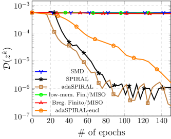
(a) Performance of different algorithms.

(b) Image recovery of adaSPIRAL.

Figure 1: Performance for the phase retrieval problem (5.2) on a digit 6 image with $N=1280$, $n=256$. Image recovery is after $100$ epochs, including the original image (left), initialization (center), and output (right).

As depicted in the figure, SPIRAL demonstrates significantly faster performance compared to the other algorithms. Even though the cost function in this scenario does not possess a Lipschitz continuous gradient, we evaluate the performance of adaSPIRAL, both in Bregman and Euclidean versions, in Figure 1(a). It is important to note that adaSPIRAL-eucl, implemented according to Algorithm 3 with the additional steps outlined in Table 1 using dgfs $h_{i}=\frac{1}{2}\|\cdot\|^{2}$, does not require any prior knowledge of Lipschitz constants $L_{i}$. Remarkably, adaSPIRAL-eucl performs well on cost functions without Lipschitz continuous gradients, as verified by this simulation. Consequently, adaSPIRAL-eucl demonstrates potential applicability to a wider range of cost functions in various applications. Additionally, adaSPIRAL outperforms SPIRAL due to its ability to employ larger stepsizes that are dynamically updated as needed, thereby speeding up convergence. Furthermore, as shown in Figure 1(b), adaSPIRAL-eucl exhibits good image recovery capabilities even in highly corrupted initial conditions.

5.3 $\ell_{1}$ Regularized Least Squares Problem

In this section, we evaluate the performance of SPIRAL for the Lasso problem, which is a convex optimization problem commonly used for regression tasks. The Lasso formulation is given by

$$\textstyle\operatorname{minimize}_{z\in\mathbb{R}^{n}}\frac{1}{2}\|Az-b\|^{2}_{2}+\lambda\|z\|_{1}$$ (5.3)

where $A$ is a matrix with data vectors $a_{i}\in\mathbb{R}^{n}$ as its rows, and $b$ is a vector with corresponding labels $b_{i}\in\mathbb{R}$. The datasets used for regression tasks include the mg, cadata, housing, and triazines datasets obtained from LIBSVM. Additionally, synthetic datasets are generated using the procedure described in [49, §6] for two different dimensions. The parameter $\lambda$ is appropriately set for each dataset.

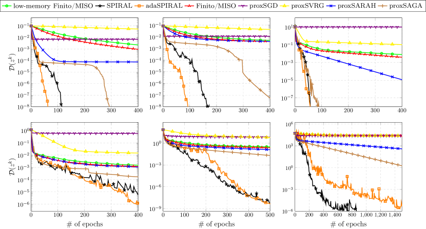
Figure 2: Performance of different algorithms for the Lasso problem (5.3). Synthetic dataset (top left) with $N=10000$, $n=400$, synthetic dataset (top center) with $N=300$, $n=600$, mg (top right) with $N=1385$, $n=6$, triazines (bottom left) with $N=186$, $n=60$, housing (bottom center) with $N=506$, $n=13$, and cadata (bottom right) with $N=20640$, $n=8$.

Figure 2 provides a comparison of different algorithms on six datasets. It is evident from the results that both SPIRAL and adaSPIRAL exhibit superior convergence performance compared to other algorithms, regardless of whether the datasets are synthetic or practical. Also the same speed up by adaSPIRAL is evident for most of the datasets. Note that adaSPIRAL does not require a priori knowledge of Lipschitz constants $L_{i}$, and still its performance is comparable with that of SPIRAL. Compared to Finito/MISO, low-memory Finito/MISO is worse, however, it does not need a large memory to store the gradient vectors. It is also observed that SPIRAL is particularly fast on dense datasets.

5.4 Nonnegative Principal Component Analysis

In this section, we investigate the problem of nonnegative principal component analysis (NN-PCA), which has also been studied in previous works [56, 53]. The problem is formulated as follows:

$$\operatorname{minimize}_{z\in\mathbb{R}^{n}}f(z)\coloneqq-\tfrac{1}{2N}\textstyle\sum_{i=1}^{N}z^{T}(a_{i}a_{i}^{T})z\quad\operatorname{subject\ to}\|z\|\leq 1,\ z\geq 0,$$ (5.4)

where $N$ denotes the number of data points represented by $a_{i}\in\mathbb{R}^{n}$. To cast the problem with the form of (1.1), we define $f_{i}(z)=-\frac{1}{2}z^{T}(a_{i}a_{i}^{T})z$ and $g(z)=\delta_{\mathcal{B}}(z)$, where $\mathcal{B}\coloneqq\{w\in\mathbb{R}^{n}\mid\|w\|\leq 1,w\geq 0\}$ represents the constraints of the NN-PCA problem (5.4). It is worth mentioning that SPIRAL allows for different smoothness constants and individualized stepsizes $\gamma_{i}$ for each of the functions $f_{i}$. In this case, the data points $a_{i}$ are not normalized to improve the output of NN-PCA analysis, providing a better representation of the dataset. All the algorithms employed for this nonconvex optimization problem are initialized with running proxSGD for 10 epochs, starting from the same initial point, ensuring convergence to a similar local optimum. The optimality criterion (5.1) is reported as a function of the number of epochs.

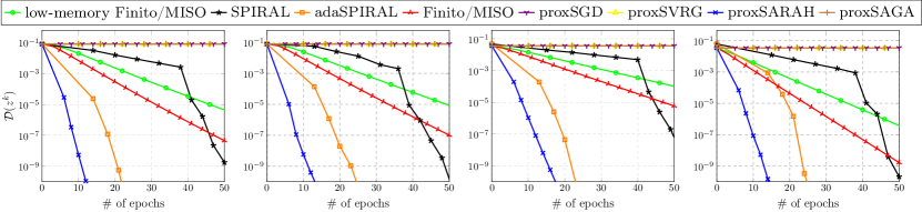
Figure 3: Performance of different algorithms for the NN-PCA problem of (5.4). MNIST (left) with $N=60000$, $n=784$, covtype (left center) with $N=581012$, $n=54$, a9a (right center) with $N=32561$, $n=123$, and aloi (right) with $N=108000$, $n=128$.

As depicted in Figure 3, the quasi-Newton updates in SPIRAL significantly enhance the convergence rate compared to (low-memory) Finito/MISO, which lacks such updates. Although proxSARAH exhibits faster convergence for this problem, it performs slower in the Lasso problem and is unable to handle non-Lipschitz differentiable cost functions, as demonstrated in the problem discussed in Section 5.2.

In order to demonstrate how competitive different versions of SPIRAL are with state-of-the-art methods used in ML, also in terms of CPU time, performance comparisons are conducted in Appendix D. It is worth noting that despite SPIRAL’s approximation of second-order information, the adopted quasi-Newton method, namely L-BFGS, demonstrates efficiency by relying solely on inexpensive level 1 BLAS operations, such as inner products, scalar multiplications, and additions.

6 Conclusion

This paper introduced SPIRAL, an optimization algorithm designed for solving regularized finite sum minimization problems. SPIRAL operates in a nonconvex setting and does not rely on the typical assumption of Lipschitz differentiability. Many existing methods that utilize quasi-Newton directions in finite sum settings either impose restrictive conditions or only achieve local convergence. In contrast, we demonstrated that SPIRAL achieves a superlinear convergence rate while ensuring global convergence, all without the need for diminishing step sizes, and under standard mild assumptions. This is achieved by the introduction of a straightforward yet effective linesearch which is smart, in the sense that it will never be triggered close enough to (sufficiently regular) solutions—an aspect validated also in our simulations. Moreover, it is observed that while addressing nonsmooth nonconvex problems, SPIRAL is still competitive with the state-of-the-art on classical convex problems, such as regularized least squares problems. Promising future research directions include the adaptation of SPIRAL to domains like distributed and federated learning.

Appendix A Preliminaries

Fact A.1 (basic properties [18, 50]).

The following hold for a dgf $H:\mathbb{R}^{n}\to\mathbb{R}$, $x,y,z\in\mathbb{R}^{n}$:

1. (three-point inequality) $\operatorname{D}_{H}(x,z)=\operatorname{D}_{H}(x,y)+\operatorname{D}_{H}(y,z)+\langle{x-y},{\nabla H(y)-\nabla H(z)}\rangle.$ [18, Lem. 3.1].

For any convex set $\mathcal{U}\subseteq\mathbb{R}^{n}$ and $u,v\in\mathcal{U}$ the following hold [50, Thm. 2.1.5, 2.1.10]:

1. If $H$ is $\mu_{H,\mathcal{U}}$-strongly convex on $\mathcal{U}$, then $\frac{\mu_{H,\mathcal{U}}}{2}\|v-u\|^{2}\leq\operatorname{D}_{H}(v,u)\leq\frac{1}{2\mu_{H,\mathcal{U}}}\|\nabla H(v)-\nabla H(u)\|^{2}$.

2. If $\nabla H$ is $\ell_{H,\mathcal{U}}$-Lipschitz on $\mathcal{U}$, then $\frac{1}{2\ell_{H,\mathcal{U}}}\|\nabla H(v)-\nabla H(u)\|^{2}\leq\operatorname{D}_{H}(v,u)\leq\frac{\ell_{H,\mathcal{U}}}{2}\|v-u\|^{2}$.

In the following, some properties of the Bregman Moreau envelope are highlighted. The interested reader is referred to [1] and [37] for proofs and further properties.

Fact A.2 (Basic properties of $\phi^{H}$ and $\operatorname{prox}_{\phi}^{H}$, [1, 37]).

Let $H:\mathbb{R}^{n}\to\mathbb{R}$ denote a dgf (cf. Definition 2.1), and $\phi:\mathbb{R}^{n}\to\overline{\mathbb{R}}$ be a proper lsc, and lower bounded function. Then, the following hold:

1. $\operatorname{prox}_{\phi}^{H}$ is locally bounded, compact-valued, and outer semicontinuous;

2. $\phi^{H}$ is finite-valued and continuous; it is locally Lipschitz if so is $\nabla H$;

3. $\phi^{H}(z)=\phi(v)+\operatorname{D}_{H}(v,z)\leq\phi(y)+\operatorname{D}_{H}(y,z)$ with any $y,z\in\mathbb{R}^{n}$, $v\in\operatorname{prox}_{\phi}^{H}(z)$. Hence, $\phi^{H}(z)\leq\phi(z)$;

4. $\inf\phi=\inf\phi^{H}$ and $\operatorname{argmin}\phi^{H}=\operatorname{argmin}\phi$;

5. $\phi^{H}$ is level-bounded iff so is $\phi$.

The following fact studies sufficient conditions for Lipschitz continuity of the Bregman proximal mapping and continuity of the Moreau envelope, both of which are crucial to the theory developed in Theorems 4.7 and 4.12.

Fact A.3 ([39, Lem. A.2]).

Let $\mathcal{V}_{i}\subseteq\mathbb{R}^{n}$ be nonempty and convex, $i\in[N]$, and let $\mathcal{V}\coloneqq\mathcal{V}_{1}\times\cdots\times\mathcal{V}_{N}$. Additionally to Assumption 1, suppose that $g$ is convex, and $h_{i}$, $i\in[N]$, is $\ell_{h_{i}}$-smooth and $\mu_{h_{i}}$-strongly convex on $\mathcal{V}_{i}$. Then, the following hold for function $\hat{H}$ as in (4.2) with $\gamma_{i}\in(0,\nicefrac{{N}}{{L_{f_{i}}}})$, $i\in[N]$:

1. $\operatorname{prox}_{\Phi}^{\hat{H}}$ is $\bar{L}$-Lipschitz continuous on $\mathcal{V}$ for some constant $\bar{L}\geq 0$.

If in addition $f_{i}$ and $h_{i}$ are twice continuously differentiable on $\mathcal{V}_{i}$, $i\in[N]$, then

1. $\Phi^{\hat{H}}$ is continuously differentiable on $\mathcal{V}$ with $\nabla\Phi^{\hat{H}}=\nabla^{2}\hat{H}\circ(\operatorname{id}-\operatorname{prox}_{\Phi}^{\hat{H}})$.

The following fact establishes the equivalence between problems (1.1) and (4.1).

Fact A.4 ([39, Lem. A.1]).

Let the functions $\varphi$ and $\Phi$ be as in (1.1) and (4.1), respectively. Then,

1. $\partial\Phi(\bm{x})=\{\bm{v}=(v,\dots,v)\mid\sum_{i}v_{i}\in\partial\varphi(x)\}$ if $\bm{x}=(x,\dots,x)\in\Delta$, and is empty otherwise.

2. $\Phi$ has the KL property at $\bm{x}=(x,\dots,x)$ iff so does $\varphi$ at $x$. In this case, the desingularizing functions are the same up to a positive scaling.

Appendix B Omitted lemmas

Lemma B.1.

Suppose that Assumptions 1 and 2 hold and that $\varphi$ is level bounded. Consider the sequence generated by Algorithm 1. Then, for every $\ell\in[N]$ there exists $c_{\ell}>0$ such that

$$\|\tilde{z}^{k}_{\ell}-u^{k}\|\leq c_{\ell}\|\tilde{z}^{k}_{1}-u^{k}\|.$$ (B.1)

Proof.

By level boundedness of $\varphi$ and Theorem 4.7, $(\bm{u}^{k})_{k\in\mathbb{N}}$, $(\bm{z}^{k})_{k\in\mathbb{N}}$, $(\tilde{z}^{k}_{i})_{k\in\mathbb{N}},i\in[N]$ are contained in a nonempty bounded set $\bm{\mathcal{U}}$. By ass:superlinear.A2, $h_{i}$ is locally strongly convex and locally Lipschitz, which along with ass:superlinear.A1 and A.3 implies that $\operatorname{prox}_{\Phi}^{\hat{H}}$ is $\bar{L}$-Lipschitz on a convex subset of $\bm{\mathcal{U}}$ for some $\bar{L}>0$. Without loss of generality and for the sake of simplicity, we assume the cyclic sweeping rule in the incremental loop, i.e., $i^{\ell}=\ell$. Note that the following proof can be easily cast into the case of cyclic sweeping without replacement. Arguing by induction, for $\ell=1$, (B.1) holds trivially. Suppose that the claim holds for some $\ell\geq 1$. Then, by triangular inequality and the definition of $\tilde{\bm{z}}^{k}_{\ell}$ in step 2.9 of Algorithm 2

$$\|\tilde{z}^{k}_{\ell+1}-u^{k}\|={} \tfrac{1}{\sqrt{N}}\|\tilde{\bm{z}}^{k}_{\ell+1}-\bm{u}^{k}\|$$

$$\leq{} \tfrac{1}{\sqrt{N}}\|\tilde{\bm{z}}^{k}_{1}-\bm{u}^{k}\|+\tfrac{1}{\sqrt{N}}\|\tilde{\bm{z}}^{k}_{\ell+1}-\tilde{\bm{z}}^{k}_{1}\|$$

$$\text{\footnotesize Lip. continuity of $\operatorname{prox}_{\Phi}^{\hat{H}}$ and \lx@cref{creftype~refnum}{tab:lifted}}\leq{} \tfrac{1}{\sqrt{N}}\|\tilde{\bm{z}}^{k}_{1}-\bm{u}^{k}\|+\tfrac{\bar{L}}{\sqrt{N}}\|\bar{\bm{z}}^{k}_{\ell+1}-\bm{u}^{k}\|$$

$$\text{\footnotesize\eqref{eq:tz_def}}\leq{} \textstyle\|\tilde{z}^{k}_{1}-u^{k}\|+\tfrac{\bar{L}}{\sqrt{N}}\sum_{j\leq\ell}\|\tilde{z}^{k}_{j}-u^{k}\|$$

$$\text{\footnotesize(induction)}\leq{} \underbracket{\textstyle\left(1+\tfrac{\bar{L}}{\sqrt{N}}\sum_{j\leq\ell}c_{j}\right)}_{\coloneqq c_{\ell+1}}\|\tilde{z}^{k}_{1}-u^{k}\|,$$

establishing (B.1). ∎

Lemma B.2.

In addition to the assumptions in Lemma B.1, suppose that the directions $d^{k}$ in step 1.6 satisfy $\|d^{k}\|\leq D\|z^{k}-v^{k}\|$ for some $D\geq 0$. Then, $\|z^{k+1}-z^{k}\|\leq C\|\bm{z}^{k}-\bar{\bm{z}}^{k-1}_{N}\|$ holds for some positive $C$.

Proof.

By the same reasoning as in Lemma B.1, $\operatorname{prox}_{\Phi}^{\hat{H}}$ is $\bar{L}$-Lipschitz continuous on a bounded convex set containing the iterates $(\bm{u}^{k})_{k\in\mathbb{N}}$, $(\bm{z}^{k})_{k\in\mathbb{N}}$, $(\tilde{z}^{k}_{i})_{k\in\mathbb{N}},i\in[N]$. It follows from the assumption on $\|d^{k}\|$ and step algLift:1:ls.a of Algorithm 2 that

$$\|\bm{z}^{k}-\bm{u}^{k}\|\leq(1-\tau_{k})\|\bm{z}^{k}-\bm{v}^{k}\|+\tau_{k}\|\bm{d}^{k}\|\leq(1-\tau_{k}+\tau_{k}D)\|\bm{z}^{k}-\bm{v}^{k}\|\leq\eta_{1}\|\bar{\bm{z}}^{k-1}_{N}-\bm{z}^{k}\|,$$ (B.2)

where $\eta_{1}=\bar{L}(1-\tau_{k}+\tau_{k}D)$ and Lipschitz continuity of the proximal mapping was used in the last inequality. Further using triangular inequality yields

$$\|\bm{u}^{k}-\bar{\bm{z}}^{k-1}_{N}\|\leq{} \|\bm{u}^{k}-\bm{z}^{k}\|+\|\bm{z}^{k}-\bar{\bm{z}}^{k-1}_{N}\|$$ (B.3)

$$\text{\footnotesize\eqref{eq:zu}}\leq{} \left(\eta_{1}+1\right)\|\bm{z}^{k}-\bar{\bm{z}}^{k-1}_{N}\|,\quad\text{and}$$

$$\|\tilde{z}^{k}_{1}-u^{k}\|={} \tfrac{1}{\sqrt{N}}\|\tilde{\bm{z}}^{k}_{1}-\bm{u}^{k}\|$$

$$\leq{} \tfrac{1}{\sqrt{N}}\|\tilde{\bm{z}}^{k}_{1}-\bm{z}^{k}\|+\tfrac{1}{\sqrt{N}}\|\bm{z}^{k}-\bm{u}^{k}\|$$

$$\text{\footnotesize Lip. continuity of $\operatorname{prox}_{\Phi}^{\hat{H}}$ and \lx@cref{creftype~refnum}{tab:lifted}}\leq{} \tfrac{\bar{L}}{\sqrt{N}}\|\bm{u}^{k}-\bar{\bm{z}}^{k-1}_{N}\|+\tfrac{1}{\sqrt{N}}\|\bm{z}^{k}-\bm{u}^{k}\|$$

$$\text{\footnotesize\eqref{eq:12}, \eqref{eq:zu}}\leq{} \tfrac{1}{\sqrt{N}}\big{(}(\bar{L}+1)\eta_{1}+\bar{L}\big{)}\|\bm{z}^{k}-\bar{\bm{z}}^{k-1}_{N}\|.$$

Using this along with triangular inequality yields

$$\textstyle\|\bar{\bm{z}}^{k}_{N}-\bm{u}^{k}\|=\sum_{\ell=1}^{N}\|\tilde{z}^{k}_{\ell}-u^{k}\|\stackrel{{\scriptstyle\text{\eqref{eq:xu}}}}{{\leq}}\sum_{\ell=1}^{N}c_{\ell}\|\tilde{z}^{k}_{1}-u^{k}\|\leq\eta_{2}\|\bm{z}^{k}-\bar{\bm{z}}^{k-1}_{N}\|,$$

where $\eta_{2}=\sum_{\ell=1}^{N}\tfrac{c_{\ell}}{\sqrt{N}}\big{(}(\bar{L}+1)\eta_{1}+\bar{L}\big{)}$. This inequality combined with (B.3) yields

$$\|z^{k+1}-z^{k}\|={} \frac{1}{\sqrt{N}}\|\operatorname{prox}_{\Phi}^{\hat{H}}(\bar{\bm{z}}^{k}_{N})-\operatorname{prox}_{\Phi}^{\hat{H}}(\bar{\bm{z}}^{k-1}_{N})\|\leq\frac{\bar{L}}{\sqrt{N}}\|\bar{\bm{z}}^{k}_{N}-\bar{\bm{z}}^{k-1}_{N}\|$$

$$\leq{} \frac{\bar{L}}{\sqrt{N}}\|\bar{\bm{z}}^{k}_{N}-\bm{u}^{k}\|+\frac{\bar{L}}{\sqrt{N}}\|\bm{u}^{k}-\bar{\bm{z}}^{k-1}_{N}\|\leq\frac{\bar{L}}{\sqrt{N}}(\eta_{1}+\eta_{2}+1)\|\bm{z}^{k}-\bar{\bm{z}}^{k-1}_{N}\|.$$

The claimed inequality follows from Lipschitz continuity of $\operatorname{prox}_{\Phi}^{\hat{H}}$ and the inclusion in step 2.3 of Algorithm 2. ∎

Appendix C Omitted proofs

Proof of Theorem 4.16

By level boundedness of $\varphi$ and Theorem 4.7, $(\bm{u}^{k})_{k\in\mathbb{N}}$, $(\bm{z}^{k})_{k\in\mathbb{N}}$, $(\tilde{z}^{k}_{i})_{k\in\mathbb{N}}$ are contained in a nonempty convex bounded set $\bm{\mathcal{U}}$, where owing to ass:superlinear.A2, $h_{i}$ and consequently $\hat{H}$ are strongly convex. It then follows from lem:3point(ii), thm:subsequential(ii), and Lemma B.2 that $\|z^{k+1}-z^{k}\|\to 0.$ Therefore, the set of limit points of $(z^{k})_{k\in\mathbb{N}}$ is nonempty compact and connected [11, Rem. 5]. By thm:subsequential(iv) and thm:subsequential(v) the limit points are stationary for $\varphi$, and $\Phi^{\hat{H}}(\bm{z}^{k})=\mathcal{L}(v^{k},z^{k})\to\varphi_{\star}$. In the trivial case $\Phi^{\hat{H}}(\bm{z}^{k})=\mathcal{L}(v^{k},z^{k})=\varphi_{\star}$ for some $k$, the claims follow from Theorem 4.7. Assume that $\Phi^{\hat{H}}(\bm{z}^{k})>\varphi_{\star}$ for $k\in\mathbb{N}$. The KL property for $\Phi$ is implied by that of $\varphi$ due to A.4, with desingularizing function $\psi(s)=\rho s^{1-\theta}$ with exponent $\theta\in(0,1)$. Let $\Omega$ denote the set of limit points of $(\bm{z}^{k}=(z^{k},\ldots,z^{k}))_{k\in\mathbb{N}}$. Since $\hat{H}$ is strongly convex, [72, Lem. 5.1] can be invoked to infer that the function $\mathcal{M}_{\hat{H}}(\bm{w},\bm{x})=\Phi(\bm{w})+\operatorname{D}_{\hat{H}}(\bm{w},\bm{x})$ also has the KL property with exponent $\nu\in\max\{\theta,\frac{1}{2}\}$ at every point $(\bm{z}^{\star},\bm{z}^{\star})$ in the compact set $\Omega\times\Omega$. Moreover, by (4.2) $\mathcal{M}_{\hat{H}}(\bm{z}^{\star},\bm{z}^{\star})=\Phi(\bm{z}^{\star})=\varphi_{\star}$ where thm:subsequential(iv) was used in the last equality. Recall that $\bm{z}^{k}\in\operatorname{prox}_{\Phi}^{\hat{H}}(\bar{\bm{z}}^{k-1}_{N})$ as in step 2.3 of Algorithm 2. Therefore, $\partial\mathcal{M}_{\hat{H}}(\bm{z}^{k},\bar{\bm{z}}^{k-1}_{N})=(\underbrace{\partial\Phi(\bm{z}^{k})+\nabla\hat{H}(\bm{z}^{k})-\nabla\hat{H}(\bar{\bm{z}}^{k-1}_{N})}_{\ni 0,\;\text{by \eqref{thm:OC} in the lifted space}},\nabla^{2}\hat{H}(\bar{\bm{z}}^{k-1}_{N})(\bar{\bm{z}}^{k-1}_{N}-\bm{z}^{k}))$, resulting in

$$\operatorname{dist}(0,\partial\mathcal{M}_{\hat{H}}(\bm{z}^{k},\bar{\bm{z}}^{k-1}_{N}))\leq\|\nabla^{2}\hat{H}(\bar{\bm{z}}^{k-1}_{N})\|\|\bar{\bm{z}}^{k-1}_{N}-\bm{z}^{k}\|\leq c\|\bar{\bm{z}}^{k-1}_{N}-\bm{z}^{k}\|$$ (C.1)

where $c=\sup_{k}\|\nabla^{2}\hat{H}(\bar{\bm{z}}^{k-1}_{N})\|>0$ is finite due to $\tilde{z}^{k}_{N}$ being bounded (cf. thm:subsequential(vi)) and continuity of $\nabla^{2}\hat{H}$. Considering (4.18) with (C.1), since $\mathcal{M}_{\hat{H}}(\bm{z}^{k},\bar{\bm{z}}^{k-1}_{N})=\Phi^{\hat{H}}(\bar{\bm{z}}^{k-1}_{N})\to\varphi$ from above, and that $(\bm{z}^{k},\bar{\bm{z}}^{k-1}_{N})_{k\in\mathbb{N}}$ is bounded and accumulates on $\Omega\times\Omega$, up to discarding iterates the following holds

$$\textstyle\psi^{\prime}\big{(}\Phi^{\hat{H}}(\bar{\bm{z}}^{k-1}_{N})-\varphi_{\star}\big{)}=\psi^{\prime}\big{(}\mathcal{M}_{\hat{H}}(\bm{z}^{k},\bar{\bm{z}}^{k-1}_{N})-\mathcal{M}_{\hat{H}}(\bm{z}^{\star},\bm{z}^{\star})\big{)}\geq\frac{1}{c\|\bar{\bm{z}}^{k-1}_{N}-\bm{z}^{k}\|},$$ (C.2)

where $\psi=\rho s^{1-\nu}$ is a desingularizing function for $\mathcal{M}_{\hat{H}}$ on $\Omega\times\Omega$. Let us define

$$\Delta_{k}\coloneqq\psi(\Phi^{\hat{H}}(\bar{\bm{z}}^{k-1}_{N})-\varphi_{\star})=\rho[\Phi^{\hat{H}}(\bar{\bm{z}}^{k-1}_{N})-\varphi_{\star}]^{1-\nu}\leq\rho[\rho(1-\nu)c\|\bar{\bm{z}}^{k-1}_{N}-\bm{z}^{k}\|]^{\frac{1-\nu}{\nu}}.$$ (C.3)

Then, $\Delta_{k}^{\frac{\nu}{1-\nu}}\leq c\rho^{\frac{1}{1-\nu}}(1-\nu)\|\bar{\bm{z}}^{k-1}_{N}-\bm{z}^{k}\|.$ Concavity of $\psi$ also implies

$$\Delta_{k}-\Delta_{k+1}\geq\psi^{\prime}(\Phi^{\hat{H}}(\bar{\bm{z}}^{k-1}_{N})-\varphi_{\star})(\Phi^{\hat{H}}(\bar{\bm{z}}^{k-1}_{N})-\Phi^{\hat{H}}(\bar{\bm{z}}^{k}_{N}))\stackrel{{\scriptstyle\text{\ref{eq:psi_dev}}}}{{\geq}}\frac{\Phi^{\hat{H}}(\bar{\bm{z}}^{k-1}_{N})-\Phi^{\hat{H}}(\bar{\bm{z}}^{k}_{N})}{c\|\bar{\bm{z}}^{k-1}_{N}-\bm{z}^{k}\|}.$$ (C.4)

On the other hand by (4.11) and (4.10)

$$\Phi^{\hat{H}}(\bar{\bm{z}}^{k+1}_{N})-\Phi^{\hat{H}}(\bar{\bm{z}}^{k}_{N})\leq-\operatorname{D}_{\hat{H}}(\bm{z}^{k+1},\bar{\bm{z}}^{k}_{N})\leq-\frac{\mu_{\hat{H}}}{2}\|\bm{z}^{k+1}-\bar{\bm{z}}^{k}_{N}\|^{2},$$ (C.5)

where lem:3point(ii) was used and $\mu_{\hat{H}}$ denotes its strong convexity modulus. Combining (C.4) and (C.5),

$$\textstyle\Delta_{k}-\Delta_{k+1}\geq\eta\|\bar{\bm{z}}^{k-1}_{N}-\bm{z}^{k}\|\geq\frac{\eta}{C}\|\bm{z}^{k+1}-\bm{z}^{k}\|,$$ (C.6)

with some constant $\eta>0$ where the last inequality follows from Lemma B.2. Hence, $(\|\bm{z}^{k+1}-\bm{z}^{k}\|)_{k\in\mathbb{N}}$ has finite length and is thus convergent. It then follows from thm:subsequential(v) that $(\bm{z}^{k})_{k\in\mathbb{N}}$ converges to a stationary point of $\varphi$. Combining (C.3) and (C.6) we have,

$$\Delta_{k+1}\leq\Delta_{k}-\alpha\Delta_{k}^{{\frac{\nu}{1-\nu}}}$$ (C.7)

with some appropriate $\alpha\geq 0$. Hence, if $\nu=\frac{1}{2}$, i.e. $\theta\in(0,\frac{1}{2}]$ for $\Phi$, in (C.7) we have $\Delta_{k+1}\leq(1-\alpha)\Delta_{k}$. As $\alpha>0$ and $\frac{\Delta_{k+1}}{\Delta_{k}}>0$, then $(1-\alpha)\in(0,1)$ concluding $\Delta_{k}$ is Q-linearly convergent to zero. By (C.3) we then conclude $(\Phi^{\hat{H}}(\bar{\bm{z}}^{k-1}_{N}))_{k\in\mathbb{N}}$ is convergent Q-linearly and by prop:Moreau_properties(iii), where we have $\varphi(z^{k})=\Phi(\bm{z}^{k})\leq\Phi^{\hat{H}}(\bar{\bm{z}}^{k-1}_{N})$, we conclude $(\varphi(z^{k}))_{k\in\mathbb{N}}$ is convergent R-linearly. Moreover, the inequality (C.6) implies that $(\|z^{k+1}-z^{k}\|)_{k\in\mathbb{N}}$ is R-linearly convergent, thus so is $(z^{k})_{k\in\mathbb{N}}$.

Appendix D CPU time

The performance results presented in Section 5 are also reported versus CPU time. According to the numerical comparisons in Figures 5, 4 and 6, the proposed algorithm features relatively cheap iterations and has comparable computational complexity per epoch compared to the other algorithms.

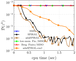
Figure 4: Performance of different algorithms versus cpu time on the phase retrieval problem (5.2) for $550$ epochs on a digit 6 image with $N=1280$, $n=256$.

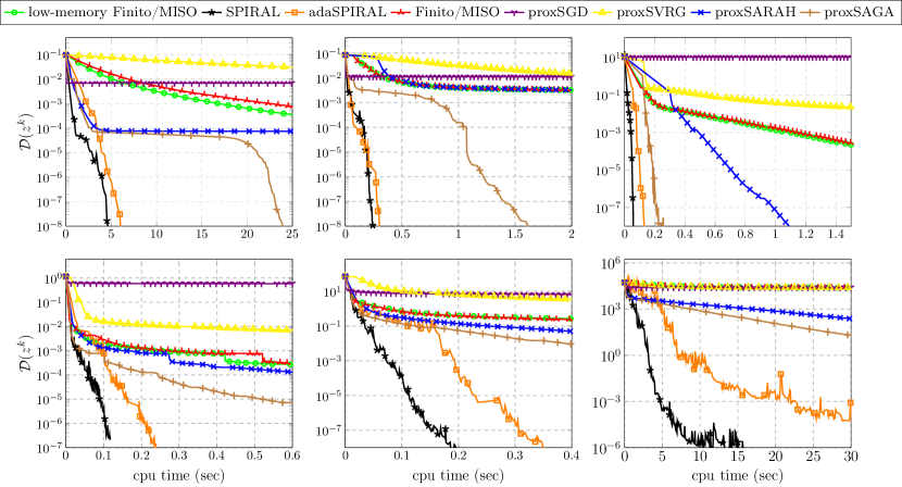
Figure 5: Performance of different algorithms versus cpu time on the lasso problem of (5.3) for $50$ epochs. Synthetic dataset (top left) with $N=10000$, $n=400$, synthetic dataset (top center) with $N=300$, $n=600$, mg (top right) with $N=1385$, $n=6$, triazines (bottom left) with $N=186$, $n=60$, housing (bottom center) with $N=506$, $n=13$, and cadata (bottom right) with $N=20640$, $n=8$.

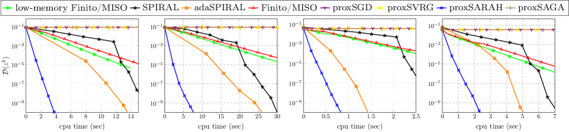
Figure 6: Performance of different algorithms versus cpu time on the NN-PCA problem of (5.4) for $500$ epochs. MNIST (left) with $N=60000$, $n=784$, covtype (left center) with $N=581012$, $n=54$, a9a (right center) with $N=32561$, $n=123$, and aloi (right) with $N=108000$, $n=128$.

Appendix E Algorithm variants

E.1 Adaptive variant

In this section, the implementation of Table 1 is further discussed. In Table 1, for the first iterate, i.e. $k=0$, the vectors $\tilde{z}^{-1}_{i}$ are initially considered equal to $z^{\rm init}$ for all $i\in[N]$. Also, note that the linesearch in step tab:3.d of Table 1 backtracks to step state:tab2.a, rather than step tab:3.c. Performing the linesearches in this intertwined fashion is observed to result in acceptance of good directions and reduction in the overall computational complexity [20, 52]. We refer the reader to [20] for the theoretical justification for the effectiveness of this procedure. Note that in Algorithm 3, in the Euclidean case, the same backtrackings can be used with dgfs $h_{i}=\frac{1}{2}\|\cdot\|^{2}$. The backtracking linesearches in the first block of Table 1 do not require storing $\tilde{z}^{k}_{i}$ and can be performed efficiently. In step state:tab1.b $\textstyle\sum_{i=1}^{N}p_{i}(\cdot,\tilde{z}^{k}_{i})$ may be evaluated by storing the scalars $\sum_{i=1}^{N}f_{i}(\tilde{z}^{k}_{i})$ and $\sum_{i=1}^{N}\langle\nabla f_{i}(\tilde{z}^{k}_{i}),\tilde{z}^{k}_{i}\rangle$ and one vector $\sum_{i=1}^{N}\nabla f_{i}(\tilde{z}^{k}_{i})\in\mathbb{R}^{n}$ while performing step 1.12 of the algorithm. Similar tricks apply to the computation of the Bregman distances, functions $p_{i}$ in other backtracking linesearches of Table 1, and updating the vectors $s^{k},\bar{s}^{k}$, and $\tilde{s}^{k}$.

E.2 Euclidean variant

Algorithm 3 SPIRAL - Euclidean version

3.1:18:

$z^{\rm init}\in\mathbb{R}^{n}$,  $\Gamma=\{\gamma_{1},\dots,\gamma_{N}\}$ with $\gamma_{i}\in(0,\nicefrac{{N}}{{L_{i}}})$, $i\in[N]$,  $\beta\in(0,1)$,

$\hat{\gamma}\coloneqq\bigl{(}\sum_{i=1}^{N}\gamma_{i}^{-1}\bigr{)}^{-1}$,  $s^{0}=z^{\rm init}-\frac{\hat{\gamma}}{N}\sum_{i=1}^{N}\nabla f_{i}(z^{\rm init})$,

maximum number of backtracks $q_{\max}\in\mathbb{N}\cup\{\infty\}$ (e.g. $q_{\max}=2$),  $K\in\mathbb{N}$

3.2:18:

3.3:18:$z^{k}\in\operatorname{prox}_{\hat{\gamma}g}(s^{k})$

3.4:18:$\bar{s}^{k}=z^{k}-\tfrac{\hat{\gamma}}{N}\sum_{i=1}^{N}\nabla f_{i}(z^{k})$ (full update)

3.5:18:$v^{k}\in\operatorname{prox}_{\hat{\gamma}g}(\bar{s}^{k})$

3.6:18:choose $d^{k}\in\mathbb{R}^{n}$ at $z^{k}$ (e.g. based on a quasi-Newton method for solving $\operatorname{r}_{\hat{h}}(z)=0$)

3.7:18:set $\tau_{k}=1,q_{k}=0$ (linesearch) a: $u^{k}=\tau_{k}z^{k}+(1-\tau_{k})v^{k}+\tau_{k}{d^{k}}$ b: $\tilde{s}^{k}=u^{k}-\tfrac{\hat{\gamma}}{N}\sum_{i=1}^{N}\nabla f_{i}(u^{k})$ (full update) c: $y^{k}\in\operatorname{prox}_{\hat{\gamma}g}(\tilde{s}^{k})$ d: if $\mathcal{L}(y^{k},u^{k})\leq\mathcal{L}(v^{k},z^{k})$ go to step 3.8 e: else if $q_{k}=q_{\rm max}$ then $u^{k}=v^{k}$,  $\tilde{s}^{k}=u^{k}-\tfrac{\hat{\gamma}}{N}\sum_{i=1}^{N}\nabla f_{i}(u^{k})$,  and go to step 3.8 f: else $\tau_{k}\leftarrow\beta\tau_{k}$,  $q_{k}\leftarrow q_{k}+1$,  and go to step alg:2:ls.a

3.8:18:$s^{k}\leftarrow\tilde{s}^{k}$

3.9:18:for  $\ell=1,\ldots,N$  do (incremental loop)

3.10:18:     randomly choose $i^{\ell}\in[N]$ without replacement

3.11:18:     $\tilde{z}^{k}_{i^{\ell}}\in\operatorname{prox}_{\hat{\gamma}g}(s^{k})$

3.12:18:     $s^{k}\leftarrow s^{k}+\tfrac{\hat{\gamma}}{N}\left(\nabla f_{{i^{\ell}}}(u^{k})-\nabla f_{{i^{\ell}}}(\tilde{z}^{k}_{i^{\ell}})\right)+\tfrac{\hat{\gamma}}{\gamma_{{i^{\ell}}}}\left(\tilde{z}^{k}_{i^{\ell}}-u^{k}\right)$

3.13:18:$s^{k+1}\leftarrow s^{k}$

3.14:18:

In this section, the proposed algorithm in the Euclidean version is outlined in Algorithm 3, when the functions $f_{i}$ have Lipschitz continuous gradients with constants $L_{i}$. In this case, the distance generating functions are $h_{i}=\frac{1}{2}\|\cdot\|^{2}$ and consequently the Bregman distances are simplified to $\operatorname{D}_{h_{i}}(y,x)=\frac{1}{2}\|y-x\|^{2}$.

References

- [1] Masoud Ahookhosh, Andreas Themelis, and Panagiotis Patrinos. A Bregman forward-backward linesearch algorithm for nonconvex composite optimization: Superlinear convergence to nonisolated local minima. SIAM Journal on Optimization, 31(1):653–685, 2021.
- [2] Francisco Javier Aragón Artacho, Anton Belyakov, Asen L Dontchev, and Marco López. Local convergence of quasi-newton methods under metric regularity. Computational Optimization and Applications, 58(1):225–247, 2014.
- [3] Heinz H Bauschke, Jérôme Bolte, and Marc Teboulle. A descent lemma beyond Lipschitz gradient continuity: first-order methods revisited and applications. Mathematics of Operations Research, 42(2):330–348, 2017.
- [4] Amir Beck and Marc Teboulle. Mirror descent and nonlinear projected subgradient methods for convex optimization. Operations Research Letters, 31(3):167–175, 2003.
- [5] Yoshua Bengio. Practical recommendations for gradient-based training of deep architectures. Neural Networks: Tricks of the Trade: Second Edition, pages 437–478, 2012.
- [6] Dimitri P. Bertsekas. Nonlinear Programming. Athena Scientific, 2016.
- [7] Dimitri P Bertsekas and John N Tsitsiklis. Gradient convergence in gradient methods with errors. SIAM Journal on Optimization, 10(3):627–642, 2000.
- [8] Doron Blatt, Alfred O Hero, and Hillel Gauchman. A convergent incremental gradient method with a constant step size. SIAM Journal on Optimization, 18(1):29–51, 2007.
- [9] Jérôme Bolte, Aris Daniilidis, and Adrian Lewis. The Łojasiewicz inequality for nonsmooth subanalytic functions with applications to subgradient dynamical systems. SIAM Journal on Optimization, 17(4):1205–1223, 2007.
- [10] Jérôme Bolte, Aris Daniilidis, Adrian Lewis, and Masahiro Shiota. Clarke subgradients of stratifiable functions. SIAM Journal on Optimization, 18(2):556–572, 2007.
- [11] Jérôme Bolte, Shoham Sabach, and Marc Teboulle. Proximal alternating linearized minimization for nonconvex and nonsmooth problems. Mathematical Programming, 146(1-2):459–494, 2014.
- [12] Jérôme Bolte, Shoham Sabach, Marc Teboulle, and Yakov Vaisbourd. First order methods beyond convexity and lipschitz gradient continuity with applications to quadratic inverse problems. SIAM Journal on Optimization, 28(3):2131–2151, 2018.
- [13] Xufeng Cai, Cheuk Yin Lin, and Jelena Diakonikolas. Empirical risk minimization with shuffled sgd: A primal-dual perspective and improved bounds. arXiv preprint arXiv:2306.12498, 2023.
- [14] Xufeng Cai, Chaobing Song, Stephen Wright, and Jelena Diakonikolas. Cyclic block coordinate descent with variance reduction for composite nonconvex optimization. In International Conference on Machine Learning, pages 3469–3494. PMLR, 2023.
- [15] Emmanuel J Candes, Xiaodong Li, and Mahdi Soltanolkotabi. Phase retrieval via Wirtinger flow: Theory and algorithms. IEEE Transactions on Information Theory, 61(4):1985–2007, 2015.
- [16] Jaeyoung Cha, Jaewook Lee, and Chulhee Yun. Tighter lower bounds for shuffling SGD: Random permutations and beyond. In International Conference on Machine Learning, pages 3855–3912. PMLR, 23–29 Jul 2023.
- [17] Chih-Chung Chang and Chih-Jen Lin. LIBSVM: A library for support vector machines. ACM transactions on intelligent systems and technology (TIST), 2:1–27, 2011.
- [18] Gong Chen and Marc Teboulle. Convergence analysis of a proximal-like minimization algorithm using Bregman functions. SIAM Journal on Optimization, 3(3):538–543, 1993.
- [19] Damek Davis, Dmitriy Drusvyatskiy, and Kellie J MacPhee. Stochastic model-based minimization under high-order growth. arXiv preprint arXiv:1807.00255, 2018.
- [20] Alberto De Marchi and Andreas Themelis. Proximal gradient algorithms under local lipschitz gradient continuity: A convergence and robustness analysis of panoc. Journal of Optimization Theory and Applications, 194(3):771–794, 2022.
- [21] Aaron Defazio, Francis Bach, and Simon Lacoste-Julien. SAGA: A fast incremental gradient method with support for non-strongly convex composite objectives. In Advances in neural information processing systems, pages 1646–1654, 2014.
- [22] Aaron Defazio and Justin Domke. Finito: A faster, permutable incremental gradient method for big data problems. In International Conference on Machine Learning, pages 1125–1133, 2014.
- [23] John E Dennis and Jorge J Moré. A characterization of superlinear convergence and its application to quasi-newton methods. Mathematics of computation, 28(126):549–560, 1974.
- [24] John E Dennis, Jr and Jorge J Moré. Quasi-newton methods, motivation and theory. SIAM review, 19(1):46–89, 1977.
- [25] Radu Alexandru Dragomir, Mathieu Even, and Hadrien Hendrikx. Fast stochastic bregman gradient methods: Sharp analysis and variance reduction. In International Conference on Machine Learning, pages 2815–2825. PMLR, 2021.
- [26] John C Duchi and Feng Ruan. Solving (most) of a set of quadratic equalities: Composite optimization for robust phase retrieval. Information and Inference: A Journal of the IMA, 8(3):471–529, 2019.
- [27] Francisco Facchinei and Jong-Shi Pang. Finite-dimensional variational inequalities and complementarity problems, volume II. Springer, 2003.
- [28] Cong Fang, Chris Junchi Li, Zhouchen Lin, and Tong Zhang. Spider: Near-optimal non-convex optimization via stochastic path-integrated differential estimator. Advances in neural information processing systems, 31, 2018.
- [29] Rong Ge, Zhize Li, Weiyao Wang, and Xiang Wang. Stabilized svrg: Simple variance reduction for nonconvex optimization. In Conference on learning theory, pages 1394–1448. PMLR, 2019.
- [30] Saeed Ghadimi and Guanghui Lan. Stochastic first-and zeroth-order methods for nonconvex stochastic programming. SIAM Journal on Optimization, 23(4):2341–2368, 2013.
- [31] Saeed Ghadimi, Guanghui Lan, and Hongchao Zhang. Mini-batch stochastic approximation methods for nonconvex stochastic composite optimization. Mathematical Programming, 155(1-2):267–305, 2016.
- [32] Mert Gürbüzbalaban, Asu Ozdaglar, and Pablo A Parrilo. Why random reshuffling beats stochastic gradient descent. Mathematical Programming, 186:49–84, 2021.
- [33] Filip Hanzely and Peter Richtárik. Fastest rates for stochastic mirror descent methods. Computational Optimization and Applications, pages 1–50, 2021.
- [34] Jeff Haochen and Suvrit Sra. Random shuffling beats sgd after finite epochs. In International Conference on Machine Learning, pages 2624–2633. PMLR, 2019.
- [35] Trevor Hastie, Jerome Friedman, and Robert Tibshirani. The Elements of Statistical Learning. Springer New York, 2001.
- [36] Rie Johnson and Tong Zhang. Accelerating stochastic gradient descent using predictive variance reduction. Advances in neural information processing systems, 26:315–323, 2013.
- [37] Chao Kan and Wen Song. The Moreau envelope function and proximal mapping in the sense of the Bregman distance. Nonlinear Analysis: Theory, Methods & Applications, 75(3):1385 – 1399, 2012.
- [38] Krzysztof Kurdyka. On gradients of functions definable in -minimal structures. Annales de l’institut Fourier, 48(3):769–783, 1998.
- [39] Puya Latafat, Andreas Themelis, Masoud Ahookhosh, and Panagiotis Patrinos. Bregman finito/miso for nonconvex regularized finite sum minimization without lipschitz gradient continuity. SIAM Journal on Optimization, 32(3):2230–2262, 2022.
- [40] Puya Latafat, Andreas Themelis, and Panagiotis Patrinos. Block-coordinate and incremental aggregated proximal gradient methods for nonsmooth nonconvex problems. Mathematical Programming, pages 1–30, 2021.
- [41] Zhize Li and Peter Richtárik. ZeroSARAH: Efficient nonconvex finite-sum optimization with zero full gradient computation. arXiv preprint arXiv:2103.01447, 2021.
- [42] Haihao Lu, Robert M. Freund, and Yurii Nesterov. Relatively smooth convex optimization by first-order methods, and applications. SIAM Journal on Optimization, 28(1):333–354, 2018.
- [43] Julien Mairal. Incremental majorization-minimization optimization with application to large-scale machine learning. SIAM Journal on Optimization, 25(2):829–855, 2015.
- [44] Konstantin Mishchenko, Ahmed Khaled, and Peter Richtárik. Random reshuffling: Simple analysis with vast improvements. Advances in Neural Information Processing Systems, 33:17309–17320, 2020.
- [45] Aryan Mokhtari, Mark Eisen, and Alejandro Ribeiro. IQN: An incremental quasi-Newton method with local superlinear convergence rate. SIAM Journal on Optimization, 28(2):1670–1698, 2018.
- [46] Aryan Mokhtari, Mert Gürbüzbalaban, and Alejandro Ribeiro. Surpassing gradient descent provably: A cyclic incremental method with linear convergence rate. SIAM Journal on Optimization, 28(2):1420–1447, 2018.
- [47] Philipp Moritz, Robert Nishihara, and Michael Jordan. A linearly-convergent stochastic L-BFGS algorithm. In Artificial Intelligence and Statistics, pages 249–258. PMLR, 2016.
- [48] Angelia Nedic and Soomin Lee. On stochastic subgradient mirror-descent algorithm with weighted averaging. SIAM Journal on Optimization, 24(1):84–107, 2014.
- [49] Yu. Nesterov. Gradient methods for minimizing composite functions. Mathematical Programming, 140(1):125–161, aug 2013.
- [50] Yurii Nesterov. Introductory lectures on convex optimization: A basic course, volume 137. Springer Science & Business Media, 2018.
- [51] Lam M Nguyen, Jie Liu, Katya Scheinberg, and Martin Takáč. SARAH: A novel method for machine learning problems using stochastic recursive gradient. In International Conference on Machine Learning, pages 2613–2621. PMLR, 2017.
- [52] Pieter Pas, Mathijs Schuurmans, and Panagiotis Patrinos. Alpaqa: A matrix-free solver for nonlinear mpc and large-scale nonconvex optimization. In 2022 European Control Conference (ECC), pages 417–422. IEEE, 2022.
- [53] Nhan H Pham, Lam M Nguyen, Dzung T Phan, and Quoc Tran-Dinh. ProxSARAH: An efficient algorithmic framework for stochastic composite nonconvex optimization. J. Mach. Learn. Res., 21:110–1, 2020.
- [54] Benjamin Recht and Christopher Ré. Parallel stochastic gradient algorithms for large-scale matrix completion. Mathematical Programming Computation, 5(2):201–226, 2013.
- [55] Sashank J. Reddi, Ahmed Hefny, Suvrit Sra, Barnabas Poczos, and Alexander J. Smola. Stochastic variance reduction for nonconvex optimization. In International conference on machine learning, pages 314–323, 2016.
- [56] Sashank J. Reddi, Suvrit Sra, Barnabas Poczos, and Alexander J. Smola. Proximal stochastic methods for nonsmooth nonconvex finite-sum optimization. In Advances in Neural Information Processing Systems, pages 1145–1153, 2016.
- [57] R. T. Rockafellar and R. J.-B. Wets. Variational analysis, volume 317. Springer Science & Business Media, 2009.
- [58] Ralph Tyrell Rockafellar. Convex analysis. Princeton University Press, 1970.
- [59] Anton Rodomanov and Dmitry Kropotov. A superlinearly-convergent proximal Newton-type method for the optimization of finite sums. In International Conference on Machine Learning, pages 2597–2605. PMLR, 2016.
- [60] Hamed Sadeghi and Pontus Giselsson. Hybrid acceleration scheme for variance reduced stochastic optimization algorithms. arXiv preprint arXiv:2111.06791, 2021.
- [61] Mark Schmidt, Nicolas Le Roux, and Francis Bach. Minimizing finite sums with the stochastic average gradient. Mathematical Programming, 162(1):83–112, mar 2017.
- [62] Shai Shalev-Shwartz and Tong Zhang. Stochastic dual coordinate ascent methods for regularized loss minimization. Journal of Machine Learning Research, 14(Feb):567–599, 2013.
- [63] Mikhail V. Solodov and Benar F. Svaiter. An inexact hybrid generalized proximal point algorithm and some new results on the theory of Bregman functions. Math. Oper. Res., 25(2):214–230, 2000.
- [64] Ju Sun, Qing Qu, and John Wright. A geometric analysis of phase retrieval. Foundations of Computational Mathematics, 18(5):1131–1198, 2018.
- [65] Marc Teboulle. A simplified view of first order methods for optimization. Mathematical Programming, 170(1):67–96, 2018.
- [66] A. Themelis and P. Patrinos. Supermann: A superlinearly convergent algorithm for finding fixed points of nonexpansive operators. IEEE Transactions on Automatic Control, 64(12):4875–4890, dec 2019.
- [67] Andreas Themelis, Masoud Ahookhosh, and Panagiotis Patrinos. On the acceleration of forward-backward splitting via an inexact Newton method. In Heinz H. Bauschke, Regina S. Burachik, and D. Russell Luke, editors, Splitting Algorithms, Modern Operator Theory, and Applications, pages 363–412. Springer International Publishing, Cham, 2019.
- [68] Andreas Themelis, Lorenzo Stella, and Panagiotis Patrinos. Forward-backward envelope for the sum of two nonconvex functions: Further properties and nonmonotone linesearch algorithms. SIAM Journal on Optimization, 28(3):2274–2303, 2018.
- [69] N Denizcan Vanli, Mert Gurbuzbalaban, and Asuman Ozdaglar. Global convergence rate of proximal incremental aggregated gradient methods. SIAM Journal on Optimization, 28(2):1282–1300, 2018.
- [70] Zhe Wang, Kaiyi Ji, Yi Zhou, Yingbin Liang, and Vahid Tarokh. Spiderboost and momentum: Faster variance reduction algorithms. Advances in Neural Information Processing Systems, 32, 2019.
- [71] Minghan Yang, Andre Milzarek, Zaiwen Wen, and Tong Zhang. A stochastic extra-step quasi-Newton method for nonsmooth nonconvex optimization. Mathematical Programming, pages 1–47, 2021.
- [72] Peiran Yu, Guoyin Li, and Ting Kei Pong. Kurdyka-Łojasiewicz exponent via inf-projection. Foundations of Computational Mathematics, pages 1–47, 2021.
- [73] Hui Zhang, Yu-Hong Dai, Lei Guo, and Wei Peng. Proximal-like incremental aggregated gradient method with linear convergence under Bregman distance growth conditions. Mathematics of Operations Research, 46(1):61–81, 2021.
- [74] Jiaojiao Zhang, Huikang Liu, Anthony Man-Cho So, and Qing Ling. Variance-reduced stochastic quasi-Newton methods for decentralized learning: Part I, 2022.