Kuramoto Networks with
Infinitely Many Stable Equilibria

Abstract.

We prove that the Kuramoto model on a graph can contain infinitely many non-equivalent stable equilibria. More precisely, we prove that for every $d\geq 1$ there is a connected graph such that the set of stable equilibria contains a manifold of dimension $d$. In particular, we solve a conjecture of R. Delabays, T. Coletta and P. Jacquod about the number of equilibria on planar graphs. Our results are based on the analysis of balanced configurations, which correspond to equilateral polygon linkages in topology. In order to analyze the stability of manifolds of equilibria we apply topological bifurcation theory.

1. Introduction.

Consider a connected graph $\mathbf{G}$ with vertices $1,\ldots,n$ and to each vertex $j$ associate a phase $\theta_{j}$ in the $1$-dimensional torus $\mathbb{T}=\mathbb{R}/2\pi\mathbb{Z}$. Let $\mathbf{N}(j)$ denote the set of neighbors of $j$ and consider the coupled dynamical system

$$\dot{\theta}_{j}=\sum_{k\in\mathbf{N}(j)}\sin(\theta_{k}-\theta_{j}),\qquad\text{for all }j=1,\ldots,n.$$ (1)

In the paper stable always means Lyapunov stable. For every graph $\mathbf{G}$ the synchronized state, in which all the phases are equal, is a stable equilibrium. It is known that other stable equilibria are present in cycles [7, 46], planar graphs [10], sparse graphs [40], $3$-regular graphs [11]. Two equilibria are equivalent if they differ by a constant. The number of non-equivalent stable equilibria is typically understood to be finite, and explicit bounds are known in some cases [10].

On the other hand, it is known that some graphs support infinitely many non-equivalent unstable equilibria. Indeed, unstable equilibria form a manifold with singularities in the case of complete graphs [6, 45, 2].

This leads to the question motivating the paper: is the number of non-equivalent stable equilibria on a connected graph always finite? Can stable equilibria form a manifold? Our main result answers these question:

Theorem 1.1.

For every $d\geq 1$ there is a connected graph $\mathbf{G}$ such that (1) contains a manifold of stable equilibria of dimension $d$.

In [10] R. Delabays, T. Coletta and P. Jacquod conjecture an upper bound on the number of non-equivalent stable equilibria in connected, planar graphs. In this paper we show that no such bound is possible, and in fact a connected, planar graph can support infinitely many non-equivalent stable equilibria:

Corollary 1.2.

The graph of Figure 1 supports infinitely many non-equivalent stable equilibria.

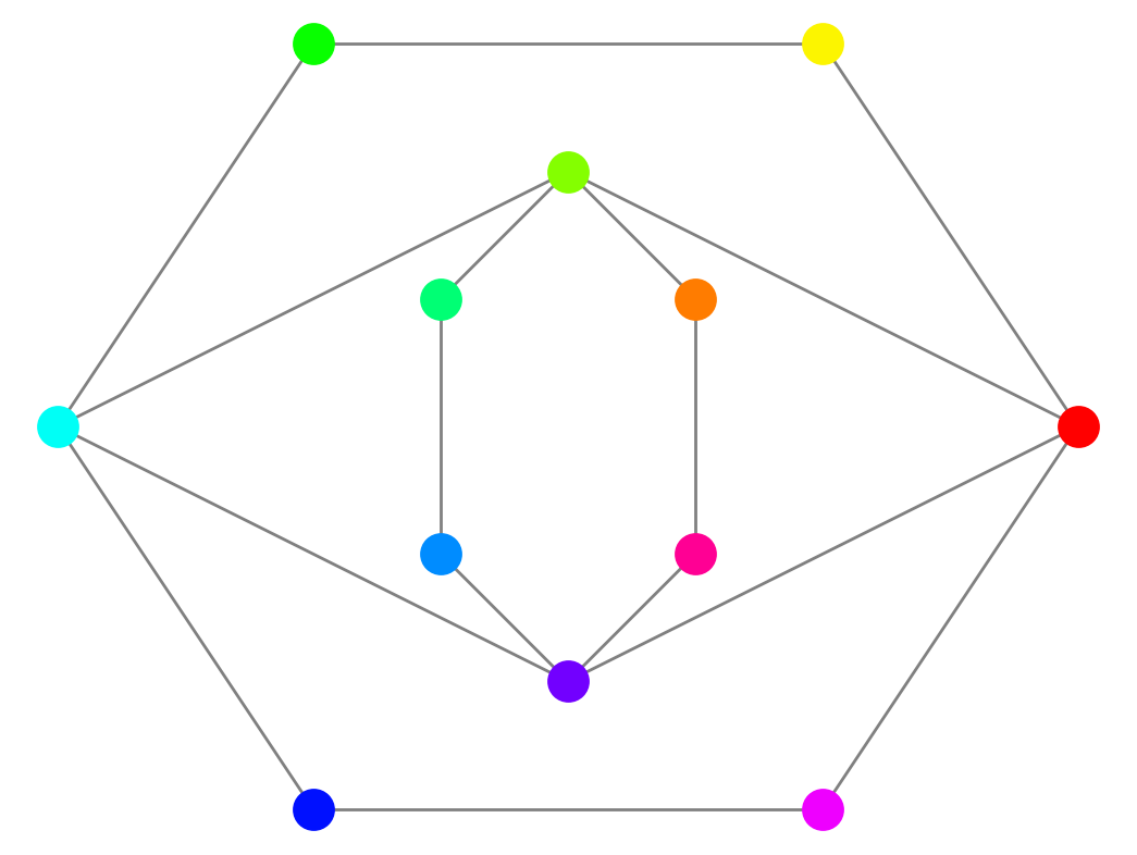
Figure 1. The eye graph supports infinitely many non-equivalent stable equilibria. A cyclic colormap is used to represent phases on vertices. The phases of the outer cycle are $(2k\pi/6)_{k=1,\ldots,6}$, starting from the rightmost vertex and proceeding counterclockwise. The phases of the inner cycle are $(2k\pi/6+\beta)_{k=1,\ldots,6}$ with $\beta=\pi/2$, starting from the topmost vertex and proceeding counterclockwise. In Section 3 we prove that a curve of non-equivalent stable equilibria is obtained by varying $\beta$ in a neighborhood of $\pi/2$.

In Section 2 we recall a known technique: algebraic geometrization. Up to a change of coordinates, the set of equilibria of (1) turns into an algebraic set. Every algebraic set is the finite union of irreducible algebraic sets; in particular, this implies that infinitely many equilibria can only appear inside a continuum of equilibria. Moreover, the system has a gradient structure: every solution is either an equilibrium or a curve joining two algebraic sets of equilibria, in the direction that makes some energy function decrease. We return to this topological/heteroclinic structure in Section 5, in which we analyze explicitly two examples of small cardinality.

Section 3 concerns balanced configurations, the main topic of the paper. We say that a subset of vertices $\mathbf{K}$ is balanced if $\sum_{k\in\mathbf{K}}e^{i\theta_{k}}=0$. As we will see, balanced configurations are able to “effectively disconnects” the network, leading to manifolds of equilibria of arbitrarily large dimension on connected graphs. The main challenge we will face is designing graphs for which these manifolds are transversally stable.

It is interesting to notice that balanced configurations appear in several areas of mathematics, although with different names. First, the quantity $\sum_{k=1}^{n}e^{i\theta_{k}}$, known as order parameter, is widely used as a measure of synchronization in phase oscillator networks [32, 34, 5, 24]. Second, balanced configurations of are known as balanced graph representations in algebraic graph theory [12]. Third, balanced configurations are in $1$-to-$1$ correspondence with equilateral polygon linkages in topology [19, 18, 21, 29].

In Section 4 we discuss aligned configurations, those in which any two phases differ by $0$ or $\pi$. They are appear in literature with different names [33, 31, 23, 44, 30, 16, 35]. In this paper we are mainly interested in the interplay between aligned configurations and balanced configurations. We prove that every equilibrium of a complete bipartite graph is a combination of these.

Our insights raise a number of questions. We know that the set of equilibria can be written as a finite union of algebraic varieties. Algebraic varieties are not necessarily manifolds, due to the presence of singular points. However:

Conjecture 1.3.

For every graph the set of equilibria of (1) is a finite union of manifolds.

Our analysis may extend to Kuramoto networks on weighted graphs, hypergraphs, or with intrinsic frequencies. A connection between the analysis of balanced configurations on weighted graph and the theory of moduli spaces in topology [20, 29, 38] is outlined in Section 3.

Finally, manifolds of stable equilibria may appear on graphs that are close to the global synchronization constant [27, 28, 41, 47], thus limiting the effectiveness of linear stability analysis as predicted in [22].

2. A System Rich in Structure.

The combinatorial structure of the underlying graph, together with the algebraic properties of the sine function, give the coupled dynamical system (1) some known, peculiar properties, which we review in detail in this section.

2.1. Phase-Shift Symmetry and Connectivity.

The equations (1) remain invariant if the same constant is added to each phase. This (dynamical) symmetry is known as phase shift and defines an action of the group $\mathbb{T}$ on the phase space $\mathbb{T}^{n}$. The phase space $\mathbb{T}^{n}$ is foliated into $(n-1)$-dimensional dynamically invariant tori. Each leaf supports the same dynamics and the group $\mathbb{T}$ acts freely on the leaves.

As a consequence, equilibria are never isolated: every equilibrium is contained in a $1$-dimensional torus of equilibria, its orbit under the group action. We say that two equilibria are equivalent if they belong to the same orbit.

If a graph is disconnected, distinct components have independent dynamics. If every connected component is endowed with a stable equilibrium, infinitely many non-equivalent stable equilibria can be obtained by phase-shifting the phases of one component. In this way we can obtain a torus of stable equilibria of dimension the number of connected components. This is a non-interesting solution to the question motivating the paper. For this reason, we will always require connectivity.

2.2. Gradient Descent.

It is well known that (1) is a gradient dynamical system [42, 27, 17]. We can write (1) as $\dot{\theta}=-\nabla E(\theta)$ where $E:\mathbb{T}^{N}\to\mathbb{R}$ is the energy function

$$E(\theta)=\sum_{jk\in\mathbf{E}(\mathbf{G})}\left(1-\cos(\theta_{j}-\theta_{k})\right).$$ (2)

Here $\mathbf{E}(\mathbf{G})$ denotes the set of edges and each edge is counted exactly once.

The identity $\dot{\theta}=-\nabla E(\theta)$ tells that a solution always evolves in the direction where the energy (2) decreases maximally. Equilibria are exactly the critical points of the energy and the only periodic trajectories. A solution is either an equilibrium or a curve joining two equilibria, traveled in the direction in which the energy decreases.

The energy function (2) is real analytic. In any real analytic gradient system the Lyapunov stable equilibria are exactly the local minima of the energy function [1]. It is interesting to notice that in a smooth (but not real analytic) gradient system this statement can fail in both ways [1].

2.3. Algebraic Geometry.

The set of equilibria of (1) is best understood in the language of algebraic geometry. For basic definitions and results we refer the reader to [14, 25, 37]. Let us identify the phase space $\mathbb{T}^{n}$ with the subset of $\mathbb{R}^{2n}$ defined by

$$x_{j}^{2}+y_{j}^{2}=1,\qquad\text{for all }j=1,\ldots,n$$ (3)

where $x_{k}=\cos(\theta_{k})$ and $y_{k}=\sin(\theta_{k})$. Then the equilibria of the system are the common solutions of (3) and

$$\sum_{k\in\mathbf{N}(j)}x_{k}y_{j}-x_{j}y_{k}=0,\qquad\text{for all }j=1,\ldots,n.$$ (4)

Therefore, the set of equilibria $X$ is an algebraic set. As such, it has a unique decomposition into irreducible components:

$$X=X_{1}\cup\ldots\cup X_{m}.$$ (5)

Each $X_{i}$ is an irreducible algebraic set (also known as algebraic variety) and none of the $X_{i}$ is contained in the union of the others. Each $X_{i}$ has a well defined dimension and tangent space at every point, except for singular points, if any.

The $1$-dimensional components in (5) are orbits of equivalent equilibria, topologically they are $1$-dimensional tori. Since the decomposition (5) is finite, we immediately learn something important about the equilibria. Either there are finitely many non-equivalent equilibria, or there is a component of dimension greater than $1$. In particular, the number of equilibria that are isolated up to phase-shift is finite.

Algebraic geometry does not prevent the existence of infinitely many non-equivalent equilibria. By contrast, it helps us understanding their geometry. The methods used in [4, 9] to prove the finiteness of the equilibria apply to a (related but) different system and only work for a generic choice of coupling coefficients.

2.4. Stability.

Every solution of (1) is either an equilibrium or a curve joining two irreducible components. A complete understanding of the system (1) requires understanding the components (5) and how they are connected by solutions.

In order to do so, we need to analyze the stability of each component. In this section we briefly review the analysis of $1$-components, which is the case already known in literature. Components of larger dimension will be analyzed in Section 3.

Since there are no isolated equilibria, throughout the paper stable will always mean Lyapunov stable.

Let $(a_{jk})_{j,k}$ denote the adjacency matrix of the graph. Fix any $\theta=(\theta_{j})_{j=1,\ldots,n}$. The component $(j,k)$ of the Jacobian matrix of the system at $\theta$ is

$$\begin{cases}a_{jk}\cos(\theta_{k}-\theta_{j})&\text{if }j\neq k\\ -\sum_{h,\,h\neq j}a_{jk}\cos(\theta_{h}-\theta_{j})&\text{if }j=k.\end{cases}$$ (6)

For every $\theta$ at least one Jacobian eigenvalue is zero; it corresponds to the direction of phase-shift $(1,\ldots,1)$.

Suppose now that $\theta$ is an equilibrium, and that exactly one eigenvalue is $0$ and the others are strictly negative. The zero eigenvalue corresponds to the direction tangent to the $1$-dimensional torus of equilibria

$$\Gamma=\{(\theta_{j}+\alpha)_{j=1,\ldots,n}\mid\alpha\in\mathbb{T}\}.$$

The zero eigenvalue disappears by restricting dynamics to the leaf containing $\theta$, in which the equilibrium is isolated. In particular $\theta$ is asymptotically stable in its leaf.

By phase shift symmetry, each equilibrium in $\Gamma$ is asymptotically stable in its leaf. The leaf locally coincides with the stable manifold of the equilibrium. These manifolds foliates the space around $\Gamma$ and intersect $\Gamma$ orthogonally (since the Jacobian (6) is symmetric).

3. Balanced Configurations and Manifolds of Equilibria.

This is the main section of the paper. For us, balanced configurations are a tool to understand manifolds of equilibria. For their role in other branches of mathematics and science we refer the reader to the introduction.

It is convenient for us to expand the notions of equilibrium and balanced configuration to a proper subset of vertices.

Definition 3.1.

A configuration is a pair consisting of a set of vertices $\mathbf{K}\subseteq\mathbf{V}(\mathbf{G})$ and a vector of phases $\theta_{\mathbf{K}}=(\theta_{k})_{k\in\mathbf{K}}$. An equilibrium of $\mathbf{K}$ is a configuration satisfying

$$\sum_{k\in\mathbf{N}(j)\cap\mathbf{K}}\sin(\theta_{k}-\theta_{j})=0,\qquad\text{for all }j\in\mathbf{K}.$$ (7)

A configuration of $\mathbf{K}$ is balanced if

$$\sum_{k\in\mathbf{K}}e^{i\theta_{k}}=0.$$ (8)

The following lemma collects some elementary properties. The proof is omitted.

Lemma 3.2.

Let $(\mathbf{K},\theta_{\mathbf{K}})$ be a configuration. The following facts are true:

1. The equilibria of $\mathbf{V}(\mathbf{G})$ according to Definition 3.1 are exactly the equilibria of the dynamical system (1);

2. For every $\alpha\in\mathbb{T}$ the configuration $\theta_{\mathbf{K}}$ is an equilibrium if and only if the configuration $\theta_{\mathbf{K}}+\alpha=(\theta_{k}+\alpha)_{k\in\mathbf{K}}$ is an equilibrium;

3. For every $\alpha\in\mathbb{T}$ the configuration $\theta_{\mathbf{K}}$ is balanced if and only if the configuration $\theta_{\mathbf{K}}+\alpha=(\theta_{k}+\alpha)_{k\in\mathbf{K}}$ is balanced;

4. Let $j$ be any vertex and suppose that $(\mathbf{K},\theta_{\mathbf{K}})$ is balanced. Then

   $$\sum_{k\in\mathbf{K}}\cos(\theta_{k}-\theta_{j})=0,$$ (9)

   $$\sum_{k\in\mathbf{K}}\sin(\theta_{k}-\theta_{j})=0.$$ (10)

Proof.

Parts $(i)$, $(ii)$, and $(iii)$ are trivial. In order to obtain $(iv)$, multiply (8) by $e^{-i\theta_{j}}$ and take real and imaginary part. This gives (9) and (10) respectively. ∎

Equation (10) tells us that the net input received by $j$ from a balanced set of neighbors is zero. This suggests how to obtain manifolds of equilibria of arbitrarily large dimension.

Lemma 3.3.

Suppose that there is a partition of the vertices of $\mathbf{G}$ into non-empty parts $\mathbf{J}_{1},\ldots,\mathbf{J}_{d}$ and a configuration $\theta=(\theta_{j})_{j=1,\ldots,n}$ such that

1. every $(\mathbf{J}_{p},\theta_{\mathbf{J}_{p}})$ is an equilibrium;

2. for every $\mathbf{J}_{p}$, $\mathbf{J}_{q}$ distinct and for every $j\in\mathbf{J}_{p}$ the set of neighbors of $j$ in $\mathbf{J}_{q}$ is balanced.

Then for every $\alpha_{1},\ldots,\alpha_{d}\in\mathbb{T}$ the configuration

$$(\theta_{\mathbf{J}_{1}}+\alpha_{1},\ldots,\theta_{\mathbf{J}_{d}}+\alpha_{1})$$ (11)

is an equilibrium of $\mathbf{G}$. In particular, the set of equilibria of $\mathbf{G}$ contains a torus of dimension $d$.

Proof.

Take any vertex $j$. Suppose that $j\in\mathbf{J}_{p}$. We have

$$\dot{\theta}_{j}=\sum_{k\in\mathbf{N}(j)\cap\mathbf{J}_{p}}\sin(\theta_{j}-\theta_{k})+\sum_{q\neq p}\sum_{k\in\mathbf{N}(j)\cap\mathbf{J}_{q}}\sin(\theta_{j}-\theta_{k}).$$

Since $\theta_{\mathbf{J}_{p}}$ is an equilibrium of $\mathbf{J}_{p}$, the first term is zero. Since $\mathbf{N}(j)\cap\mathbf{J}_{q}$ is balanced for every $q\neq p$, by (10) the second term is zero. This shows that $\theta$ is an equilibrium of $\mathbf{G}$. The statement now follows from Lemma 3.2(ii) and Lemma 3.2(iii). ∎

Let $\Gamma\subseteq\mathbb{T}^{n}$ be the $d$-dimensional torus of equilibria (11). In general, not all the equilibria in $\Gamma$ have the same stability. As we will see, by varying $\alpha_{1},\ldots,\alpha_{d}$ some Jacobian eigenvalues can change sign. This phenomenon is a particular case of topological bifurcation [26]. In the following proof we construct graphs for which a non-empty open subset of $\Gamma$ is transversally stable.

Figure 2. This figure illustrates the graph $\mathbf{G}_{5}$.

Proof of Theorem 1.1.

The idea is connecting a family of stable $6$-cycle configurations in a way that they only interact through balanced subsets. Let us begin with a $6$-cycle and phases $(2k\pi/6+\alpha)_{k=1,\ldots,6}$. Since $\cos(2\pi/6)=1/2$ the Jacobian matrix (6) is

$$\small\begin{pmatrix}-1&\frac{1}{2}&0&0&0&\frac{1}{2}\\ \frac{1}{2}&-1&\frac{1}{2}&0&0&0\\ 0&\frac{1}{2}&-1&\frac{1}{2}&0&0\\ 0&0&\frac{1}{2}&-1&\frac{1}{2}&0\\ 0&0&0&\frac{1}{2}&-1&\frac{1}{2}\\ \frac{1}{2}&0&0&0&\frac{1}{2}&-1\end{pmatrix}.\normalsize$$ (12)

Notice that it is independent of $\alpha$. Moreover, notice that the matrix is circulant. The eigenvalues of circulant matrices are easy to compute [43, 13]. In this case the characteristic polynomial is

$$p(\lambda)=\lambda(\lambda+1/2)^{2}(\lambda+3/2)^{2}(\lambda+2).$$

Exactly one eigenvalue is zero and the others are strictly negative. As $\alpha$ can vary in $\mathbb{T}$ we obtain a $1$-dimensional torus of stable equilibria. The zero eigenvalue corresponds to the tangent space of this torus.

Notice that, in this configuration, any pair of opposite vertices of the $6$-cycle is a balanced configuration. This suggests how to connect several $6$-cycles together.

Consider $d$ disjoint $6$-cycles and add an edge between the first and fourth vertex of the first cycle with the first and fourth vertex of every other cycle. This amounts to adding $4(d-1)$ edges. Let $\mathbf{G}_{d}$ denote the resulting graph. The graph $\mathbf{G}_{2}$ is the eye graph of Figure 1 of the introduction. The graph $\mathbf{G}_{5}$ is given in Figure 2.

Let $\alpha_{1},\ldots,\alpha_{d}\in\mathbb{T}$ and let $(2k\pi/6+\alpha_{i})_{k=1,\ldots,6}$ be the phases of the $i$-th cycle. The $6$-cycles only interact with each other through balanced pair of vertices. By Lemma 3.3 as $\alpha_{1},\ldots,\alpha_{d}$ vary in $\mathbb{T}$ these configurations form a $d$-dimensional torus of equilibria $\Gamma$.

In order to analyze stability, we look at Jacobian eigenvalues. We want to show that there is an open set of $(\alpha_{1},\ldots,\alpha_{d})\in\mathbb{T}^{d}$ for which exactly $d$ Jacobian eigenvalues are $0$ and the others strictly are negative.

In order to do so, we choose $\alpha_{1}=0$ and $\alpha_{2}=\ldots,\alpha_{d}=\pi/2$. Every edge between two $6$-cycles has phase difference $\pi/2$, and since $\cos(\pi/2)=0$ it follows that the Jacobian matrix is a block diagonal matrix with $d$ blocks all equal to (12). In particular the characteristic polynomial is

$$p(\lambda)^{d}=\lambda^{d}(\lambda+1/2)^{2d}(\lambda+3/2)^{2d}(\lambda+2)^{d}.$$

Notice that $0$ has multiplicity $d$ and every other eigenvalue is strictly negative.

Since $d$ is the dimension of the tangent space of $\Gamma$, it follows that there is a neighborhood of $(0,\pi/2,\ldots,\pi/2)\in\mathbb{T}^{d}$ in which exactly $d$ eigenvalues are zero and all the others are strictly negative.

Let us summarize what we have. There is a non-empty open subset $V$ of $\Gamma$ with the following properties: $V$ is a $d$-dimensional manifold, every point in $V$ is an equilibrium, the stable manifold of every such equilibrium has codimension $d$ and is orthogonal to $V$. The last statement holds since the Jacobian matrix (6) is symmetric.

By Shoshitaishvili Theorem [26, 39] the stable manifolds form a foliation of the space near $V$. It follows that every $\theta\in V$ is a Lyapunov stable equilibrium. Indeed, a point near $\theta$ lies in either the stable manifold of $\theta$ or the stable manifold of a nearby equilibrium. ∎

3.1. Stable Tori.

In the proof of Theorem 1.1 we obtain a torus of equilibria $\Gamma$, but only a proper subset is stable. Indeed, for $d=2$ we can see in Figure 3 that as the phase difference between the two cycles vary, an eigenvalue crosses zero; stability is only guaranteed in a neighborhood of $\pi/2$. We now provide several graphs in which the set of stable equilibria contain an entire $2$-dimensional torus. Due to the size of the graphs, the eigenvalues are computed numerically.

(a)

(b)

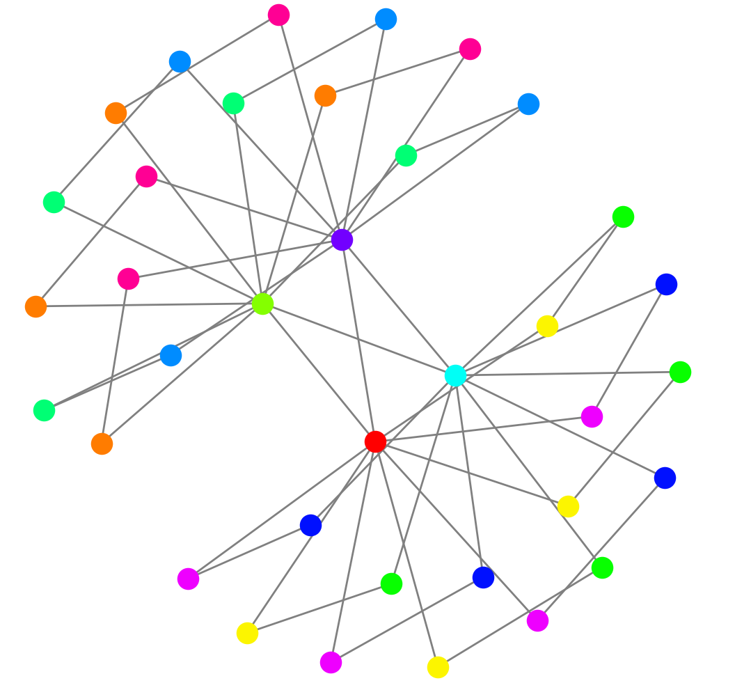
(c)

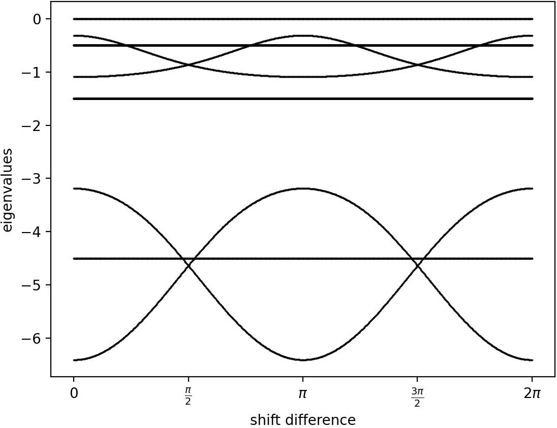
(d)

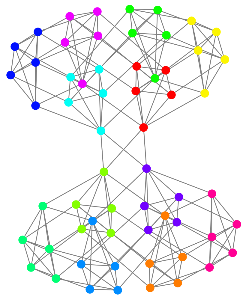
(e)

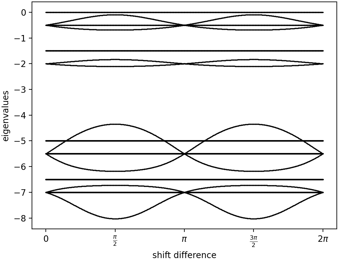
(f)

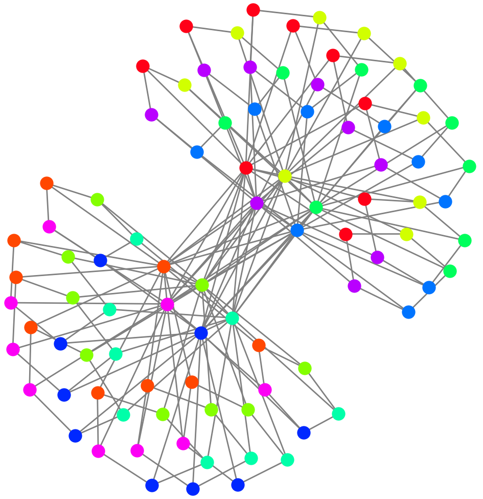
(g)

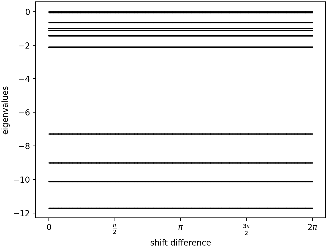
(h)

Figure 3. On the left, graphs supporting $2$-dimensional manifold of stable equilibria. On the right, eigenvalues as the phase-shift difference $\beta-\alpha$ vary.

Let us denote by $\mathbf{H}_{36}$, $\mathbf{H}_{60}$ and $\mathbf{H}_{90}$ the graphs (C), (E), and (G) of Figure 3, according to the number of vertices. The vertices have been positioned so as to highlight the division into two subsets. Each $\mathbf{H}_{36}$, $\mathbf{H}_{60}$, $\mathbf{H}_{90}$ supports a $2$-dimensional torus of stable equilibria. The torus is obtained by phase-shifting the two parts.

Let us describe the configurations in more detail. The graph $\mathbf{H}_{36}$ is obtained from the eye graph $\mathbf{G}_{2}$ by taking of each $6$-cycle $3$ copies of itself and glueing them at the pair of vertices constituting the balanced configuration. One part has phases $(2k\pi/6+\alpha)_{k=1,\ldots,6}$, the other part $(2k\pi/6+\beta)_{k=1,\ldots,6}$. Due to phase shift symmetry, stability only depends on the phase difference $\beta-\alpha$. As shown in Figure 3, for every $\alpha,\beta\in\mathbb{T}$ all non-zero eigenvalues are strictly negative. As in the proof of Theorem 1.1, by Shoshitaishvili Theorem it follows that for every $\alpha,\beta\in\mathbb{T}$ this is a stable equilibrium.

Similarly $\mathbf{H}_{60}$ is obtained from $\mathbf{G}_{2}$ by substituting each vertex with a tetrahedron and connecting the tetrahedra in parallel along the $6$-cycles.

By contrast, the graph $\mathbf{H}_{90}$ is a bit different. It is obtained by fully connecting two $5$-cycles with phases $(2k\pi/5+\alpha)_{k=1,\ldots,5}$ and $(2k\pi/5+\beta)_{k=1,\ldots,5}$ respectively. Notice that each cycle is a balanced configuration. In order to make the configuration stable, each cycle is copied $8$ times and connected in parallel to its copies. It is interesting to notice that in this case the eigenvalues do not depend on $\alpha,\beta$, see (H).

3.2. Symmetry is not Necessary.

Although the graphs discussed in this article are symmetric, symmetry is not necessary for manifolds of stable equilibria. Instead, it is useful for keeping the discussion as self-contained as possible, as symmetric graphs can be described more easily in words.

We can enlarge a stable configuration of a graph by connecting by an edge each vertex to an asymmetric graph whose phases are synchronized with that vertex. The enlarged configuration is stable. We can choose the auxiliary graphs so that the enlarged graph is asymmetric. If the original graph supports a $d$-dimensional manifolds of stable equilibria, so does the enlarged one.

3.3. The Geometry of Balanced Configurations.

We are interested in the geometry of the set of balanced configurations of $n$ vertices.

Two vertices are balanced if and only if the phases differ by $\pi$. Therefore, balanced configurations of two vertices form a $1$-dimensional torus.

There are two balanced configurations with $3$ vertices up to phase shift, corresponding to two non-equivalent labeling of the vertices of an equilateral triangle, thus leading to two disjoint $1$-dimensional tori.

Balanced configurations of $4$ vertices are given by three non-equivalent relabeling of the family $(\alpha,\beta,\alpha+\pi,\beta+\pi)_{\alpha,\beta\in\mathbb{T}}$:

$$B_{1} =\{(\alpha,\alpha+\pi,\beta,\beta+\pi)\mid\alpha,\beta\in\mathbb{T}\},$$

$$B_{2} =\{(\alpha,\beta,\alpha+\pi,\beta+\pi)\mid\alpha,\beta\in\mathbb{T}\},$$

$$B_{3} =\{(\alpha,\beta,\beta+\pi,\alpha+\pi)\mid\alpha,\beta\in\mathbb{T}\}.$$

These $2$-dimensional tori intersect at aligned configurations. Up to phase shift, the set of balanced configurations is homeomorphic to three mutually tangent circles.

Until now, every balanced configuration is somewhat symmetric. For $n\geq 5$ the situation is far more complicated, as the symmetry is lost. Using Morse Theory it has been shown that, up to phase shift, balanced configurations of $5$ vertices form a surface of genus $4$ [15, 18]. It is interesting that the separation between the case $n\leq 4$ and the case $n\geq 5$ in terms of symmetry becomes evident in terms of dynamics if the sine function is replaced by a generic function [2, Proposition 2].

In topology, balanced configurations appear in a different but equivalent form. As noticed in [3], we can associate to any balanced configuration an equilateral polygon. Let $(\theta_{k})_{k=1,\ldots,n}$ be a balanced configuration and $u_{m}=\sum_{k=1}^{m}e^{i\theta_{k}}$. Then the sequence $u_{1},\ldots,u_{n}$ defines an equilateral polygon. Here the term polygon must be taken somewhat loosely, since we allow vertices to coincide and edges to intersect.

The space of equilateral polygons is studied, for example, in [19]. Translating the results of [19] back into our language, we can rephrase Theorem A as follows:

Theorem 3.4 (Y.Kamiyama).

Let $n\geq 3$. For an odd $n$ the set of balanced configurations is a smooth manifold of dimension $n-2$. For an even $n$ the set of balanced configurations is a manifold with singular points, the generic dimension is $n-2$ and the singular points are exactly the aligned configurations.

Recall that aligned configurations are those in which any two phases differ by $0$ or $\pi$. Notice that configuration that are both balanced and aligned are only possible if $n$ is even. The presence of singular points for an even $n$ is already evident for $n=4$, at the aforementioned tori $B_{1}$, $B_{2}$, $B_{3}$ intersect. We conjecture that for every $n\geq 3$ the set of balanced configurations is a branched manifold and can be written as a union of smooth manifolds.

As already noticed, balanced configurations correspond to equilateral polygons. In the theory of moduli spaces [20, 29, 38] non-equilateral polygons are considered, usually with generic edge lengths. This may be useful in better understanding the Kuramoto model on weighted graphs.

4. Aligned Configurations and Complete Bipartite Graphs.

In this section we discuss synchronized and aligned equilibria. We are mainly interested in the case of complete bipartite graphs, where balanced and aligned configurations characterize all the equilibria. For our purposes, it is convenient to expand these notions to a proper subset of vertices.

Definition 4.1.

A configuration of $\mathbf{K}$ is aligned if the points $\{e^{i\theta_{k}}\}_{k\in\mathbf{K}}$ belong to a line passing through the origin of $\mathbb{C}$, that is, any two phases differ by $0$ or $\pi$. If all the phases are equal we say that $\mathbf{K}$ is synchronized.

Unlike balanced configurations, the aligned configuration of $\mathbf{V}(\mathbf{G})$ is an equilibrium for every $\mathbf{G}$. We refer to these configurations as aligned equilibria. There are $2^{n-1}$ non-equivalent aligned equilibria, each corresponding to a $1$-dimensional torus. As we will see in a later section, some of them may be part of larger component. Notice that there is only one synchronized equilibrium up to phase-shift.

Proposition 4.2.

Let $\mathbf{G}$ be connected. Then the only stable aligned equilibria of $\mathbf{G}$ are the synchronized equilibria.

Proof.

Let $\theta$ be an aligned equilibrium. The vertices $\mathbf{V}(\mathbf{G})$ can be partitioned into two subsets $\mathbf{J}$ and $\mathbf{K}$ such that every vertex in $\mathbf{J}$ have phase $\alpha$ and every vertex in $\mathbf{K}$ have phase $\alpha+\pi$, for some $\alpha\in\mathbb{T}$. Let $\mathbf{E}(\mathbf{J},\mathbf{K})$ denote the set of edges between $\mathbf{J}$ and $\mathbf{K}$ and $\left|\mathbf{E}(\mathbf{J},\mathbf{K})\right|$ the cardinality of this set.

Suppose that $\theta$ is not a synchronized equilibrium, then $\mathbf{J}$ and $\mathbf{K}$ are non-empty. Since $\mathbf{G}$ is connected the set $\mathbf{E}(\mathbf{J},\mathbf{K})$ is non-empty. Perturb $\theta$ as $\tilde{\theta}_{k}=\theta_{k}+x$ for $k\in\mathbf{K}$ and $\tilde{\theta}_{j}=\theta_{j}$ for $j\in\mathbf{J}$. We claim that that the energy (2) decreases in the direction of the perturbation. Indeed

$$E(\theta)-E(\tilde{\theta}) =\sum_{jk\in\mathbf{E}(\mathbf{G})}\cos(\tilde{\theta}_{j}-\tilde{\theta}_{k})-\cos(\theta_{j}-\theta_{k})$$

$$=\sum_{jk\in\mathbf{E}(\mathbf{J},\mathbf{K})}\cos(\tilde{\theta}_{j}-\tilde{\theta}_{k})-\cos(\theta_{j}-\theta_{k})$$

$$=\left|\mathbf{E}(\mathbf{J},\mathbf{K})\right|(\cos(\pi+x)-\cos(\pi))$$

and since $\left|\mathcal{E}(\mathbf{J},\mathbf{K})\right|$ is positive the difference $E(\theta)-E(\tilde{\theta})$ is positive for every $x$ small enough. The equilibrium $\theta$ is not a local minimum, and thus it is not stable.

It remains to prove that the synchronized equilibria are stable. This follows from the fact that, for every graph $\mathbf{G}$, synchronized equilibria are exactly the global minima of the energy (2). ∎

4.1. Complete Bipartite Graphs.

In order to show how balanced configurations and aligned configurations may interplay, we discuss complete bipartite graphs. In [8] it is shown that the synchronized configurations are the only stable equilibria in complete bipartite graph. Here we complete the analysis by classifying all the possible equilibria, with a focus on their geometric structure. In particular, we see that balanced configurations lead to manifolds of unstable equilibria of arbitrarily large dimension.

Proposition 4.3.

Let $\mathbf{G}$ be complete bipartite with non-empty parts $\mathbf{J}$ and $\mathbf{K}$. The equilibria of $\mathbf{G}$ have the following form:

1. $\theta_{\mathbf{J}}$ is balanced, $\theta_{\mathbf{K}}$ is balanced;

2. $\theta_{\mathbf{J}}$ is not balanced, $\theta_{\mathbf{K}}$ is balanced and aligned to $\sum_{j\in\mathbf{J}}e^{i\theta_{j}}$;

3. $\theta_{\mathbf{K}}$ is not balanced, $\theta_{\mathbf{J}}$ is balanced and aligned to $\sum_{j\in\mathbf{K}}e^{i\theta_{k}}$;

4. $\theta$ is aligned.

Proof.

It is easy to see that every configuration of $\mathbf{V}(\mathbf{G})$ satisfying any of the conditions (i) through (iv) is an equilibrium.

Conversely, let $\theta$ be an equilibrium. We prove that $\theta$ satisfies at least one of the conditions. We have

$$\Im\left(\sum_{k\in\mathbf{K}}e^{i\theta_{k}}e^{-i\theta_{j}}\right)=0,\qquad\text{for all }j\in\mathbf{J};$$ (13)

$$\Im\left(\sum_{j\in\mathbf{J}}e^{i\theta_{j}}e^{-i\theta_{k}}\right)=0,\qquad\text{for all }k\in\mathbf{K}.$$ (14)

If $\mathbf{J}$ and $\mathbf{K}$ are both balanced we are in case (i). Suppose that $\mathbf{J}$ is not balanced. Due to the phase-shift symmetry, we can assume that $\sum_{j\in\mathbf{J}}e^{i\theta_{j}}$ is real and strictly positive. From (14) it follows that $\theta_{k}\in\{0,\pi\}$ for every $k\in\mathbf{K}$. Then from (13) it follows that either $\mathbf{K}$ has an even number of vertices, half with phase $0$ and half with phase $\pi$, and we are in case (ii), or $\theta_{j}\in\{0,\pi\}$ for every $j\in\mathbf{J}$, and we are in case (iv). Similarly, if $\mathbf{K}$ is not balanced we are in case (iii) or in case (iv). ∎

Let $\left|\mathbf{J}\right|=n$ and $\left|\mathbf{K}\right|=m$. Suppose that $n,m\geq 3$. By Theorem 3.4 the set of equilibria of the form (i) has dimension $(n-2)(m-2)$. The set of equilibria of the form (ii) has dimension $n$ if $m$ is even and is empty otherwise. Similarly, the set of equilibria of the form (iii) has dimension $m$ if $n$ is even and is empty otherwise. The aligned configurations (ii) form a set of dimension $1$.

Notice that the cases (i) through (iv) are not disjoint and the conditions (ii) and (iii) are not closed. Therefore, in order to obtain the decomposition in irreducible components some more work is needed. In the next section we give an explicit example.

5. Manifolds Connected by Heteroclinic Orbits

A heteroclinic orbit is a solution joining two equilibria. We know from Section 2 that every solution of (1) is either an equilibrium or a heteroclinic orbit connecting two irreducible sets of equilibria. Given a graph, we are led to the following program:

• computing the irreducible decomposition of the set of equilibria;

• establishing how the components are connected by solutions.

As we will see by two examples, even for small graphs this program may lead to some intricate topological structures.

5.1. Complete graph with $4$ vertices.

Consider a complete graphs with vertices $\mathbf{V}(\mathbf{G})=\{1,2,3,4\}$. The only equilibria are the balanced configurations of $\mathbf{V}(\mathbf{G})$ and the aligned configurations of $\mathbf{V}(\mathbf{G})$. As explained in Section 3 the balanced configurations of four vertices are arranged into three $2$-dimensional tori:

$$B_{1} =\{(\alpha,\alpha+\pi,\beta,\beta+\pi)\mid\alpha,\beta\in\mathbb{T}\},$$

$$B_{2} =\{(\alpha,\beta,\alpha+\pi,\beta+\pi)\mid\alpha,\beta\in\mathbb{T}\},$$

$$B_{3} =\{(\alpha,\beta,\beta+\pi,\alpha+\pi)\mid\alpha,\beta\in\mathbb{T}\}.$$

These tori mutually intersect at aligned balanced configurations. Up to phase-shift the balanced configurations form three mutually tangent circles. There are only three aligned balanced configurations up to phase-shift. The energy of the balanced configurations is $E=8$, which is the maximum of the system.

The aligned configurations that are not balanced are

$$A_{1}=\{(\alpha,\alpha+\pi,\alpha+\pi,\alpha+\pi)\mid\alpha\in\mathbb{T}\},$$

$$A_{2}=\{(\alpha+\pi,\alpha,\alpha+\pi,\alpha+\pi)\mid\alpha\in\mathbb{T}\},$$

$$A_{3}=\{(\alpha+\pi,\alpha+\pi,\alpha,\alpha+\pi)\mid\alpha\in\mathbb{T}\},$$

$$A_{4}=\{(\alpha+\pi,\alpha+\pi,\alpha+\pi,\alpha)\mid\alpha\in\mathbb{T}\},$$

with energy $E=6$, and the synchronized state

$$S=\{(\alpha,\alpha,\alpha,\alpha)\mid\alpha\in\mathbb{T}\}$$

with energy $E=0$. By perturbing the phase of one vertex, it is easy to see that the equilibria in $A_{1}$, $A_{2}$, $A_{3}$, and $A_{4}$ are not local maxima nor local minima.

A heteroclinic connection is only possible from a set with higher energy to a set with lower energy. Numerically, we see that any connection allowed by the energy actually exists. The existence of an orbit between $A_{i}$ and $S$ is trivial since $S$ is the global minimum of the energy. In order to establish the existence of an orbit between $A_{i}$ and $B_{j}$, we perturbed an equilibrium of $A_{i}$ and applied the Runge–Kutta method RK4 with reversed time. We obtain the heteroclinic structure of Figure 4.

Figure 4. Topology of the set of equilibria up to phase shift of the complete graph with $4$ vertices. A dotted arrow represents the existence of a heteroclinic orbit.

5.2. Cycle with $4$ vertices.

A cycle graph with vertices $1$, $2$, $3$, $4$ is a complete bipartite graph with parts $\mathbf{J}=\{1,3\}$ and $\mathbf{K}=\{2,4\}$. Therefore, we can apply Proposition 4.3. Equilibria of the form (i), in which each part is balanced, constitute a $2$-dimensional torus

$$B_{2}=\{(\alpha,\beta,\alpha+\pi,\beta+\pi)\mid\alpha,\beta\in\mathbb{T}\}$$

with energy $E=4$. Equilibria of the form (ii) and (iii), in which one part is generic and the other is balanced and aligned give the $2$-dimensional tori

$$C_{1} =\{(\beta-\delta,\beta,\beta+\delta,\beta+\pi)\mid\beta,\delta\in\mathbb{T}\},$$

$$C_{2} =\{(\alpha,\alpha+\delta,\alpha+\pi,\alpha-\delta)\mid\alpha,\delta\in\mathbb{T}\},$$

with energy $E=4$. Notice that the conditions (ii) and (iii) are not closed, here we are taking closures. It is easy to see that the equilibria in $B_{2}$, $C_{1}$ and $C_{2}$ are not local maxima nor local minima.

Notice that $B_{2}$, $C_{1}$ and $C_{2}$ contain two aligned equilibria each. The remaining aligned equilibria are

$$A_{5} =\{(\alpha,\alpha+\pi,\alpha,\alpha+\pi)\mid\alpha\in\mathbb{T}\},$$

$$S =\{(\alpha,\alpha,\alpha,\alpha)\mid\alpha\in\mathbb{T}\},$$

with energy $E=8$ and $E=0$ respectively. Therefore, we obtain the heteroclinic network of Figure 5.

Notice that $B_{2}$, $C_{1}$ and $C_{2}$ intersect in two $1$-dimensional tori. The equilibria in the intersection have the property that all Jacobian eigenvalues are zero. Equilibria with this property, known as completely degenerate, correspond to the Eulerian circuits in the graph [36]. In this case, the intersections correspond to the two ways of traveling around the cycle.

Figure 5. Topology of the set of equilibria up to phase shift of the cycle graph with $4$ vertices. A dotted arrow represents the existence of a heteroclinic orbit.

References

- [1] P. A. Absil and K. Kurdyka, On the stable equilibrium points of gradient systems, Systems and Control Letters, 55 (2006), pp. 573–577.
- [2] P. Ashwin, C. Bick, and O. Burylko, Identical phase oscillator networks: Bifurcations, symmetry and reversibility for generalized coupling, Frontiers in Applied Mathematics and Statistics, 2 (2016), p. 7.
- [3] P. Ashwin, O. Burylko, and Y. Maistrenko, Bifurcation to heteroclinic cycles and sensitivity in three and four coupled phase oscillators, Physica D: Nonlinear Phenomena, 237 (2008), pp. 454–466.
- [4] J. Baillieul and C. Byrnes, Geometric critical point analysis of lossless power system models, IEEE Transactions on Circuits and Systems, 29 (1982), pp. 724–737.
- [5] C. Bick, M. Timme, D. Paulikat, D. Rathlev, and P. Ashwin, Chaos in symmetric phase oscillator networks, Physical review letters, 107 (2011), p. 244101.
- [6] E. Brown, P. Holmes, and J. Moehlis, Globally coupled oscillator networks, in Perspectives and Problems in Nolinear Science, Springer, 2003, pp. 183–215.
- [7] E. Canale and P. Monzon, Global properties of kuramoto bidirectionally coupled oscillators in a ring structure, in 2009 IEEE Control Applications,(CCA) & Intelligent Control,(ISIC), IEEE, 2009, pp. 183–188.
- [8] E. A. Canale and P. A. Monzon, On the characterization of families of synchronizing graphs for kuramoto coupled oscillators, IFAC Proceedings Volumes, 42 (2009), pp. 42–47.
- [9] T. Chen, R. Davis, and D. Mehta, Counting Equilibria of the Kuramoto Model Using Birationally Invariant Intersection Index, SIAM Journal on Applied Algebra and Geometry, 2 (2018), pp. 489–507.
- [10] R. Delabays, T. Coletta, and P. Jacquod, Multistability of phase-locking in equal-frequency kuramoto models on planar graphs, Journal of Mathematical Physics, 58 (2017), p. 032703.
- [11] L. DeVille and B. Ermentrout, Phase-locked patterns of the Kuramoto model on 3-regular graphs, Chaos, 26 (2016), pp. 1–11.
- [12] C. Godsil and G. F. Royle, Algebraic graph theory, vol. 207, Springer Science & Business Media, 2001.
- [13] R. M. Gray, Toeplitz and circulant matrices: A review, (2006).
- [14] R. Hartshorne, Algebraic geometry, vol. 52, Springer Science & Business Media, 2013.
- [15] T. Havel, The use of distances as coordinates in computer-aides proofs of theorems in euclidean geometry, J. Symbolic Comput., 11 (1991), pp. 579–593.
- [16] J. M. Hendrickx and J. N. Tsitsiklis, Convergence of type-symmetric and cut-balanced consensus seeking systems, IEEE Transactions on Automatic Control, 58 (2012), pp. 214–218.
- [17] A. Jadbabaie, N. Motee, and M. Barahona, On the stability of the kuramoto model of coupled nonlinear oscillators, in Proceedings of the 2004 American Control Conference, vol. 5, IEEE, 2004, pp. 4296–4301.
- [18] Y. Kamiyama, An elementary proof of a theorem of tf havel, Ryukyu Math. J, 5 (1992), pp. 7–12.
- [19] , Topology of equilateral polygon linkages, Topology and its Applications, 68 (1996), pp. 13–31.
- [20] M. Kapovich and J. Millson, On the moduli space of polygons in the euclidean plane, Journal of Differential Geometry, 42 (1995), pp. 133–164.
- [21] M. Kapovich and J. J. Millson, The symplectic geometry of polygons in euclidean space, Journal of Differential Geometry, 44 (1996), pp. 479–513.
- [22] M. Kassabov, S. H. Strogatz, and A. Townsend, Sufficiently dense Kuramoto networks are globally synchronizing, Chaos: An Interdisciplinary Journal of Nonlinear Science, 31 (2021), p. 073135.
- [23] N. Kopell and D. Somers, Anti-phase solutions in relaxation oscillators coupled through excitatory interactions, Journal of mathematical biology, 33 (1995), pp. 261–280.
- [24] Y. Kuramoto and I. Nishikawa, Statistical macrodynamics of large dynamical systems. case of a phase transition in oscillator communities, Journal of Statistical Physics, 49 (1987), pp. 569–605.
- [25] S. Lang, Introduction to algebraic geometry, Courier Dover Publications, 2019.
- [26] S. Liebscher, Bifurcation without parameters, vol. 526, Springer, 2015.
- [27] S. Ling, R. Xu, and A. S. Bandeira, On the landscape of synchronization networks: A perspective from nonconvex optimization, SIAM Journal on Optimization, 29 (2019), pp. 1879–1907.
- [28] J. Lu and S. Steinerberger, Synchronization of kuramoto oscillators in dense networks, Nonlinearity, 33 (2020), p. 5905.
- [29] A. Mandini, The duistermaat-heckman formula and the cohomology of moduli spaces of polygons, Journal of Symplectic Geometry, 12 (2014), pp. 171–213.
- [30] J. Markdahl, Counterexamples in synchronization: pathologies of consensus seeking gradient descent flows on surfaces, Automatica, 134 (2021), p. 109945.
- [31] E. A. Martens, C. Bick, and M. J. Panaggio, Chimera states in two populations with heterogeneous phase-lag, Chaos: An Interdisciplinary Journal of Nonlinear Science, 26 (2016), p. 094819.
- [32] R. E. Mirollo, The asymptotic behavior of the order parameter for the infinite-n kuramoto model, Chaos: An Interdisciplinary Journal of Nonlinear Science, 22 (2012), p. 043118.
- [33] Y. Park and B. Ermentrout, Weakly coupled oscillators in a slowly varying world, Journal of computational neuroscience, 40 (2016), pp. 269–281.
- [34] D. Pazó, Thermodynamic limit of the first-order phase transition in the kuramoto model, Physical Review E, 72 (2005), p. 046211.
- [35] W. Ren and R. W. Beard, Consensus seeking in multiagent systems under dynamically changing interaction topologies, IEEE Transactions on automatic control, 50 (2005), pp. 655–661.
- [36] D. Sclosa, Completely degenerate equilibria of the kuramoto model on networks, arXiv preprint arXiv:2112.12034, (2021).
- [37] I. R. Shafarevich and M. Reid, Basic algebraic geometry, vol. 2, Springer, 1994.
- [38] D. Shimamoto and C. Vanderwaart, Spaces of polygons in the plane and morse theory, The American Mathematical Monthly, 112 (2005), pp. 289–310.
- [39] A. N. Shoshitaishvili, Bifurcations of topological type at singular points of parametrized vector fields, Funktsional’nyi Analiz i ego Prilozheniya, 6 (1972), pp. 97–98.
- [40] Y. Sokolov and G. B. Ermentrout, When is sync globally stable in sparse networks of identical kuramoto oscillators?, Physica A: Statistical Mechanics and its Applications, 533 (2019), p. 122070.
- [41] R. Taylor, There is no non-zero stable fixed point for dense networks in the homogeneous kuramoto model, Journal of Physics A: Mathematical and Theoretical, 45 (2012), p. 055102.
- [42] J. Van Hemmen and W. Wreszinski, Lyapunov function for the kuramoto model of nonlinearly coupled oscillators, Journal of Statistical Physics, 72 (1993), pp. 145–166.
- [43] R. S. Varga, Eigenvalues of circulant matrices, Pacific J. Math, 4 (1954), pp. 151–160.
- [44] G. Vathakkattil Joseph and V. Pakrashi, Limits on anti-phase synchronization in oscillator networks, Scientific Reports, 10 (2020), pp. 1–9.
- [45] S. Watanabe and J. W. Swift, Stability of periodic solutions in series arrays of josephson junctions with internal capacitance, Journal of nonlinear science, 7 (1997), pp. 503–536.
- [46] D. A. Wiley, S. H. Strogatz, and M. Girvan, The size of the sync basin, Chaos: An Interdisciplinary Journal of Nonlinear Science, 16 (2006), p. 015103.
- [47] R. Yoneda, T. Tatsukawa, and J. N. Teramae, The lower bound of the network connectivity guaranteeing in-phase synchronization, Chaos, 31 (2021).