SP2 : A Second Order Stochastic Polyak Method

Abstract

Recently the SP (Stochastic Polyak step size) method has emerged as a competitive adaptive method for setting the step sizes of SGD. SP can be interpreted as a method specialized to interpolated models, since it solves the interpolation equations. SP solves these equation by using local linearizations of the model. We take a step further and develop a method for solving the interpolation equations that uses the local second-order approximation of the model. Our resulting method SP2 uses Hessian-vector products to speed-up the convergence of SP. Furthermore, and rather uniquely among second-order methods, the design of SP2 in no way relies on positive definite Hessian matrices or convexity of the objective function. We show SP2 is very competitive on matrix completion, non-convex test problems and logistic regression. We also provide a convergence theory on sums-of-quadratics.

1 Introduction

Consider the problem

$$w^{*}\in\operatorname{argmin}_{w\in\mathbb{R}^{d}}\left\{f(w):=\frac{1}{n}\sum_{i=1}^{n}f_{i}(w)\right\},$$ (1)

where $f$ is twice continuously differentiable, and the set of minimizers is nonempty. Let the optimal value of (1) be $f^{*}\in\mathbb{R}$, and $w^{0}$ be a given initial point. Here each $f_{i}(w)$ is the loss of a model parametrized in $w\in\mathbb{R}^{d}$ over an $i$-th data point. Our discussion, and forth coming results, also hold for a loss given as an expectation $f(w)=\mathbf{E}_{\xi\sim{\cal D}}\left[f_{\xi}(w)\right]$, where $\xi\sim{\cal D}$ is the data generating process and $f_{\xi}(w)$ the loss over this sampled data point. But for simplicity we use the $f_{i}(w)$ notation.

Contrary to classic statistical modeling, there is now a growing trend of using overparametrized models that are able to interpolate the data [24]; that is, models for which the loss is minimized over every data point as described in the following assumption.

Assumption 1.1.

We say that the interpolation condition holds when the loss is nonnegative, $f_{i}(w)\geq 0$, and

$$\exists~{}w^{*}\in\mathbb{R}^{d}\quad\mbox{such that}\quad f(w^{*})=0.$$ (2)

Consequently, $f_{i}(w^{*})=0$ for $i=1,\ldots,n$.

Overparameterized deep neural networks are the most notorious example of models that satisfy Assumption 1.1. Indeed, with sufficiently more parameters than data points, we are able to simultaneously minimize the loss over all data points.

If we admit that our model can interpolate the data, then we have that our optimization problem (1) is equivalent to solving the system of nonlinear equations

$$f_{i}(w)\;=\;0,\quad\mbox{for }i=1,\ldots,n.$$ (3)

Since we assume $f_{i}(w)\geq 0$ any solution to the above is a solution to our original problem.

Recently, it was shown in [13] that the Stochastic Polyak step size (SP) method [4, 23, 30] directly solves the interpolation equations. Indeed, at each iteration SP samples a single $i$-th equation from (3), then projects the current iterate $w^{t}$ onto the linearization of this constraint, that is

$$w^{t+1}=\operatorname{argmin}_{w\in\mathbb{R}^{d}}\left\|w-w^{t}\right\|^{2}\quad\mbox{ s.t. }f_{i}(w^{t})+\left<\nabla f_{i}(w^{t}),w-w^{t}\right>=0.$$ (4)

The closed form solution to (4) is given by

$$w^{t+1}=w^{t}-\tfrac{f_{i}(w^{t})}{\left\|\nabla f_{i}(w^{t})\right\|^{2}}\nabla f_{i}(w^{t}).$$ (5)

Here we take one step further, and instead of projecting onto the linearization of $f_{i}(w)$ we use the local quadratic expansion. That is, as a proxy of setting $f_{i}(w)=0$ we set the quadratic expansion of $f_{i}(w)$ around $w^{t}$ to zero

$$f_{i}(w^{t})+\left<\nabla f_{i}(w^{t}),w-w^{t}\right>+\tfrac{1}{2}\left<\nabla^{2}f_{i}(w^{t})(w-w^{t}),w-w^{t}\right>=0.$$ (6)

The above quadratic constraint could have infinite solutions, a unique solution or no solution at all. Indeed, for example if $\nabla^{2}f_{i}(w^{t})$ is positive definite, there may exist no solution, which occurs when $f_{i}$ is convex, and is the most studied setting for second order methods. But if the loss is positive $f_{i}$ and the Hessian has at least one negative eigenvalue, then (6) always has a solution.

If (6) has solutions, then analogously to the SP method, we can choose one using a projection step

$$w^{t+1}\;\in\; \operatorname{argmin}_{w\in\mathbb{R}^{d}}\tfrac{1}{2}\left\|w-w^{t}\right\|^{2}$$

$$\mbox{ s.t. }f_{i}(w^{t})+\left<\nabla f_{i}(w^{t}),w-w^{t}\right>+\tfrac{1}{2}\left<\nabla^{2}f_{i}(w^{t})(w-w^{t}),w-w^{t}\right>=0.$$ (7)

We refer to (7) as the SP2 method. Using a quadratic expansion has several advantages. First, quadratic expansions are more accurate than linearizations, which will allow us to take larger steps. Furthermore, using the quadratic expansion will lead to convergence rates which are independent on how well conditioned the Hessian matrices are, as we show later in Proposition 4.1.

Our SP2 method occupies a unique position in the literature of stochastic second order method since it is incremental and in no way relies on convexity or positive semi-definite Hessian matrices. Indeed, as we will show in our non-convex experiments in 6.1 and matrix completition B, the SP2 excels at minimizing non-convex problems that satisfy interpolation. In contrast, Newton based methods often converge to stationary points other than the global minima.

We also relax the interpolation assumption, and develop analogous quadratic methods for finding $w$ and the smallest possible $s\in\mathbb{R}$ such that

$$f_{i}(w)\;\leq\;s,\quad\mbox{for }i=1,\ldots,n.$$ (8)

We refer to this as the slack interpolation equations, which were introduced in [9] for linear models. If the interpolation assumption holds then $s=0$ and the above is equivalent to solving (3). When interpolation does not hold, then (8) is still a upper approximation of (1), as detailed in [12].

The rest of this paper is organized as follows. We introduce some related work in Section 2. We present the proposed SP2 methods in Section 3 and corresponding convergence analysis in Section 4. In Section 5, we relax the interpolation condition and develop a variety of quadratic methods to solve the slack version of this problem. We test the proposed methods with a series of experiments in Section 6. Finally, we conclude our work and discuss future directions in Section 7.

2 Related Work

Since it became clear that Stochastic Gradient Descent (SGD), with appropriate step size tuning, was an efficient method for solving the training problem (1), there has been a search for an efficient second order counter part. The hope being, and our objective here, is to find a second order stochastic method that is incremental; that is, it can work with mini-batches, requires little to no tuning since it would depend less on how well scaled or conditioned the data is, and finally, would also apply to non-convex problems. To date there is a vast literature on stochastic second order methods, yet none that achieve all of the above.

The subsampled Newton methods such as [33, 5, 22, 11, 20, 17] require large batch sizes in order to guarantee that the subsampled Newton direction is close to the full Newton direction in high probability. As such are not incremental. Other examples of large sampled based methods include the Stochastic quasi-Newton methods [6, 26, 27, 14, 36, 3], stochastic cubic Newton [35], SDNA [31], Newton sketch [29] and Lissa [1], since these require a large mini-batch or full gradient evaluations.

The only incremental second order methods we aware of are IQN (Incremental Quasi-Newton) [25], SNM (Stochastic Newton Method) [21, 32] and very recently SAN (Stochastic Average Newton) [7]. IQN and SNM enjoy a fast local convergence, but their computational and memory costs per iteration, is of ${\cal O}(d^{2})$ making them prohibitive in large dimensions.

Handling non-convexity in second order methods is particularly challenging because most second order methods rely on convexity in their design. For instance, the classic Newton iteration is the minima of the local quadratic approximation if this approximation is convex. If it is not convex, the Newton step can be meaningless, or worse, a step uphill. Quasi-Newton methods maintain positive definite approximation of the Hessian matrix, and thus are also problematic when applied to non-convex problems [36] for which the Hessian is typically indefinite. Furthermore the incremental Newton methods IQN, SNM and SAN methods rely on the convexity of $f_{i}$ in their design. Indeed, without convexity, the iterates of IQN, SNM and SAN are not well defined.

In contrast, our approach of finding roots of the local quadratic approximation (7) in no way relies on convexity, and relies solely on the fact that the local quadratic approximation around $w^{t}$ is good if we are not far from $w^{t}.$ But our approach does introduce a new problem: the need to solve a system of quadratic equations. We propose a series of methods to solve this in Sections 3 and 5.

Solving quadratic equations has been heavily studied. There are even dedicated methods for solving

$$w^{\star}=\operatorname*{argmin}_{w\in\mathbb{R}^{d}}\tfrac{1}{2}\|w-\bar{w}\|^{2}~{}\mbox{ s.t. }Q(w)=0,\text{ where }Q({w})=\tfrac{1}{2}{w}^{\top}{\bf H}{w}+b^{\top}{w}+c$$ (9)

for a given $\bar{w}$, where ${\bf H}$ is a nonzero symmetric (not necessarily PSD) matrix, and the level set $\{w:Q(w)=0\}$ is nonempty. Note that since $Q(w)$ is a quadratic function, the problem (9) is nonconvex. Yet despite this non-convexity, so long as there exists a feasible point, the projection (9) can be solved in polynomial time by re-writing the projection as a semi-definite program, or by using the S-procedure, which involves computing the eigenvalue decomposition of ${\bf H}$ and using a line search as proposed in  [28], and detailed here in Section A.1. But this approach is too costly when the dimension $d$ is large.

An alternative iterative method is proposed in [34], but only asymptotic convergence is guaranteed. In [10], the authors consider a similar problem by projecting a point onto a general ellipsoid, which is again a problem of solving quadratic equations. However, they require the matrix ${\bf H}$ to be a positive definite matrix.

The problem (7) and (9) are also an instance of a quadratic constrained quadratic program (QCQP). Although the QCQP in (7) has no closed form solution in general, we show in the next section that there is a closed form solution for Generalized linear models (GLMs), that holds for convex and non-convex GLMs alike. For general non-linear models we propose in Section 3.2 an approximate solution to (7) by iteratively linearizing the quadratic constraint and projecting onto the linearization.

3 The SP2 Method

Next we give a closed form solution to (7) for GLMs. We then provide an approximate solution to (7) for more general models.

3.1 SP2⁺ - Generalized Linear Models

Consider when $f_{i}$ is the loss over a linear model with

$$f_{i}(w)=\phi_{i}(x_{i}^{\top}w-y_{i}),$$ (10)

where $\phi_{i}:\mathbb{R}\rightarrow\mathbb{R}$ is a loss function, and $(x_{i},y_{i})\in\mathbb{R}^{d+1}$ is an input-output pair. Consequently

$$\nabla f_{i}(w)=\phi_{i}^{\prime}(x_{i}^{\top}w-y_{i})x_{i}\coloneqq a_{i}x_{i},\qquad\nabla^{2}f_{i}(w)=\phi_{i}^{\prime\prime}(x_{i}^{\top}w-y_{i})x_{i}x_{i}^{\top}\coloneqq h_{i}x_{i}x_{i}^{\top}.$$ (11)

The quadratic constraint problem (7) can be solved exactly for GLMs (10) as we show next.

Lemma 3.1.

(SP2) Assume $f_{i}(w)$ is the loss of a generalized linear model (10) and is non-negative. Let $f_{i}=f_{i}(w^{t})$ for short. Let $a_{i}\coloneqq\phi_{i}^{\prime}(x_{i}^{\top}w-y_{i})$ and $h_{i}\coloneqq\phi_{i}^{\prime\prime}(x_{i}^{\top}w-y_{i})$. If

$$a_{i}^{2}-2h_{i}f_{i}\geq 0$$ (12)

then the optimal solution of (7) is as follows

$$w^{t+1} =w^{t}-\frac{a_{i}}{h_{i}}\left(1-\frac{\sqrt{a_{i}^{2}-2h_{i}f_{i}}}{|a_{i}|}\right)\frac{x_{i}}{\|x_{i}\|^{2}}.$$ (13)

Alternatively if (12) does not hold, since $f_{i}\geq 0$ we have necessarily that $h_{i}>0$, and consequently a Newton step will give the minima of the local quadratic, that is

$$w^{t+1} =w^{t}-\frac{a_{i}}{h_{i}}\frac{x_{i}}{\left\|x_{i}\right\|^{2}}.$$ (14)

The proof to the above lemma, and all subsequent missing proofs can be found in the appendix. Lemma (3.1) establishes a condition (12) under which we should not take a full Newton step. Interestingly, this condition (12) holds when the square root of the loss function has negative curvature, as we show in the next lemma.

Lemma 3.2.

Let $\phi$ be a non-negative function which is twice differentiable at all $t$ with $\phi(t)\neq 0$. The condition (12), in other words

$$\phi^{\prime}(t)^{2}\geq 2\phi(t)\phi^{\prime\prime}(t)$$

holds when $\sqrt{\phi(t)}$ is concave away from its roots, i.e. when $\frac{d^{2}}{dt^{2}}\sqrt{\phi(t)}\leq 0$ for all $t$ with $\phi(t)\neq 0.$

Figure (a) Non-convex loss func. for which condition (12) holds.

Examples of loss functions include $\phi(t)=\tanh^{2}{(t)}$ and $\phi(t)=t^{p}$ with $0\leq p\leq 2$ (see Figure (a)).

In conclusion to this section, SP2 has a closed form solution for GLMs, and this closed form solution includes many non-convex loss functions.

3.2 SP2⁺ - Linearizing and Projecting

In general, there is no closed form solution to (7). Indeed, there may not even exist a solution. Inspired by the fact that computing a Hessian-vector product can be done with a single backpropagation at the same cost as computing a gradient [8], we will make use of the cheap Hessian-vector product to derive an approximate solution to (7).

Instead of solving (7) exactly, here we propose to take two steps towards solving (7) by projecting onto the linearized constraints. To describe this method let

$$q(w)\coloneqq f_{i}(w^{t})+\left<\nabla f_{i}(w^{t}),w-w^{t}\right>+\tfrac{1}{2}\left<\nabla^{2}f_{i}(w^{t})(w-w^{t}),w-w^{t}\right>.$$ (15)

In the first step we linearize the quadratic constraint (15) around $w^{t}$ and project onto this linearization:

$$w^{t+1/2}= \operatorname{argmin}_{w\in\mathbb{R}^{d}}\tfrac{1}{2}\left\|w-w^{t}\right\|^{2}\quad\mbox{ s.t. }f_{i}(w^{t})+\left<\nabla f_{i}(w^{t}),w-w^{t}\right>=0.$$ (16)

The closed form update of this first step is given by

$$w^{t+1/2} = w^{t}-\frac{f_{i}(w^{t})}{\left\|\nabla f_{i}(w^{t})\right\|^{2}}\nabla f_{i}(w^{t}),$$ (17)

which is a Stochastic Polyak step (5). For the second step, we once again linearize the quadratic constraint (15), but this time around the point $w^{t+1/2}$ and set this linearization to zero, that is

$$w^{t+1}= \operatorname{argmin}_{w\in\mathbb{R}^{d}}\tfrac{1}{2}\!\left\|w-w^{t+1/2}\right\|^{2}~{}~{}\mbox{s.t. }q(w^{t+1/2})+\left<\nabla q(w^{t+1/2}),w-w^{t+1/2}\right>=0.$$ (18)

The closed form update of this second step is given by

$$w^{t+1}=w^{t+1/2}-\frac{q(w^{t+1/2})}{\left\|\nabla q(w^{t+1/2}))\right\|^{2}}\nabla q(w^{t+1/2}).$$ (19)

We refer to the resulting proposed method as the SP2⁺ method, summarized in the following.

Lemma 3.3.

(SP2⁺) Let $g_{t}\equiv\nabla f_{i}(w^{t})$ and ${\bf H}_{t}\equiv\nabla^{2}f_{i}(w^{t})$. Update (17) and (19) is given by

$$w^{t+1}\!=w^{t}\!-\frac{f_{i}(w^{t})}{\left\|g_{t}\right\|^{2}}g_{t}\!-\frac{1}{2}\frac{f_{i}(w^{t})^{2}}{\left\|g_{t}\right\|^{4}}\frac{\left<{\bf H}_{t}g_{t},g_{t}\right>}{\left\|v^{t+1}\right\|^{2}}v^{t+1},\;\mbox{where}\;v^{t+1}\;=\left({\bf I}-{\bf H}_{t}\frac{f_{i}(w^{t})}{\left\|g_{t}\right\|^{2}}\right)g_{t},$$ (20)

In (20) we can see that SP2⁺ applies a second order correction to the SP step.

SP2⁺ is equivalent to two steps of a Newton Raphson method applied to finding a root of $q(w)$. If we apply multiple steps of the Newton Raphson method, as opposed to two, the resulting method converges to the root of $q$, see Theorem C.1 in the appendix. Theorem C.1 shows that this multi-step version of SP2⁺ converges when $q$ belongs to a large class of non-convex functions known as the star-convex functions. Star-convexity, which is a generalization of convexity, includes several non-convex loss functions [16].

4 Convergence Theory

Here we provide a convergence theory for SP2 and SP2⁺ for when $f(w)$ is an average of quadratic functions. Let $w^{*}\in\operatorname{argmin}_{w\in\mathbb{R}^{d}}f(w)$ and let the loss over the $i$-th data point be given by

$$f_{i}(w)=\left<{\bf H}_{i}(w-w^{*}),w-w^{*}\right>,$$ (21)

where ${\bf H}_{i}\in\mathbb{R}^{d\times d}$ is a symmetric positive semi-definite matrix for $i=1,\ldots,n.$ Consequently $f_{i}(w^{*})=0=f(w^{*})=\min_{w\in\mathbb{R}^{d}}f(w),$ thus the interpolation condition holds.

Proposition 4.1.

Consider the loss functions given in (21). The SP2 method (7) converges linearly

$$\mathbb{E}\left[\left\|w^{t+1}-w^{*}\right\|^{2}\right]\leq\rho\;\mathbb{E}\left[\left\|w^{t}-w^{*}\right\|^{2}\right],\quad\text{where}\;\rho=\lambda_{\max}\left({\bf I}-\frac{1}{n}\sum_{i=1}^{n}{\bf H}_{i}{\bf H}_{i}^{+}\right)<1.$$ (22)

The rate of convergence of SP2 in (22) can be orders of magnitude better than SGD. Indeed, since (21) is convex, smooth and interpolation holds, we have from [15] that SGD converges at a rate of

$$\rho_{SGD}=1-\frac{1}{2n}\frac{\lambda_{\min}(\sum_{i=1}^{n}{\bf H}_{i})}{\max_{i=1,\ldots,n}\lambda_{\max}({\bf H}_{i})}.$$ (23)

To compare (23) to $\rho$ rate in Proposition 4.1, consider the case where all ${\bf H}_{i}$ are invertible. In this case ${\bf H}_{i}{\bf H}_{i}^{+}={\bf I}$ and thus $\rho=0$ and SP2 converges in one step. Indeed, even if a single ${\bf H}_{i}$ is invertible, after sampling $i$ the SP2 will converge. In contrast, the SGD method is still at the mercy of the spectra of the ${\bf H}_{i}$ matrices and depend on how well conditioned these matrices are. Even in the extreme case where all ${\bf H}_{i}$ are well conditioned, for example ${\bf H}_{i}=i\times{\bf I}$, the rate of convergence of SGD can be very slow, for instance in this case we have $\rho_{SGD}~{}=~{}1~{}-~{}\frac{1}{2n^{2}}.$

Proposition 4.2.

Consider the loss functions in (21). The SP2⁺ method (20) converges linearly

$$\mathbb{E}\left[\left\|w^{t+1}-w^{*}\right\|^{2}\right]\leq\rho_{SP2^{+}}^{2}\;\mathbb{E}\left[\left\|w^{t}-w^{*}\right\|^{2}\right],\;\text{where}\;\rho_{SP2+}=1-\frac{1}{2n}\sum_{i=1}^{n}\frac{\lambda_{\min}({\bf H}_{i})}{\lambda_{\max}({\bf H}_{i})}.$$ (24)

The rate of convergence of SP2⁺ now depends on the average condition number of the ${\bf H}_{i}$ matrix. Yet still, the rate of convergence in (24) is always better than that of SGD. Indeed, this follows because of the maximum over the index $i$ in (23) and since

$$\frac{1}{2n}\sum_{i=1}^{n}\frac{\lambda_{\min}({\bf H}_{i})}{\lambda_{\max}({\bf H}_{i})}\geq\frac{1}{2n}\sum_{i=1}^{n}\frac{\lambda_{\min}({\bf H}_{i})}{\max_{i=1,\ldots,n}\lambda_{\max}({\bf H}_{i})}.$$

Note also that the rate of SP2⁺ appears squared in (24) and the rate $\rho_{SGD}$ of SGD is not squared. But this difference accounts for the fact that each step of SP2⁺ is at least twice the cost of SGD, since each step of SP2⁺ is comprised of two gradient steps, see (17) and (19). Thus we can neglect the apparent advantage of the rate $\rho_{SP2+}$ being squared.

5 Quadratic with Slack

Here we depart from the interpolation Assumption 1.1 and design a variant of SP2⁺ that can be applied to models that are close to interpolation. Instead of trying to set all the losses to zero, we now will try to find the smallest slack variable $s>0$ for which

$$f_{i}(w)\leq s,\quad\mbox{ for }i=1,\ldots,n.$$

If interpolation holds, then $s=0$ is a solution. Outside of interpolation, $s$ may be non-zero.

5.1 L2 slack formulation

To make $s$ as small as possible, we can solve the following problem

$$\min_{s\in\mathbb{R},w\in\mathbb{R}^{s}}\frac{1}{2}s^{2}\mbox{ subject to }f_{i}(w)\leq s,\mbox{ for }i=1,\ldots,n,$$ (25)

which is called the L2 slack formulation. This type of slack problem was introduced in [9] to derive variants of the passive-aggressive method that could be applied to linear models on non-separable data, in other words, that do not interpolate the data.

To solve (25) we will again project onto a local quadratic approximation of the constraint. Let

$$q_{i,t}(w)\coloneqq f_{i}(w^{t})+\left<\nabla f_{i}(w^{t}),w-w^{t}\right>+\tfrac{1}{2}\left<\nabla^{2}f_{i}(w^{t})(w-w^{t}),w-w^{t}\right>.$$ (26)

and let $\Delta_{t}=\left\|w-w^{t}\right\|^{2}+(s-s^{t})^{2}.$ Consider the iterative method given by

$$w^{t+1},s^{t+1}= \underset{s\geq 0,\;w\in\mathbb{R}^{d}}{\operatorname{argmin}}\frac{1-\lambda}{2}\Delta_{t}+\frac{\lambda}{2}s^{2}\quad\mbox{ s.t. }q_{i,t}(w)\leq s,$$ (27)

where $\lambda\in[0,\;1]$ is a regularization parameter that trades off between having a small $s$, and using the previous iterates as a regularizor. The resulting projection problem in (27) has a quadratic inequality, and thus in most cases has no closed form solution, despite always being feasible.

So instead of solving (27) exactly, we propose an approximate solution by iteratively linearizing and projecting onto the constraints. Our approximate solution has two steps, the first step being

$$w^{t+1/2},s^{t+1/2}= \underset{s\geq 0,\;w\in\mathbb{R}^{d}}{\operatorname{argmin}}\frac{1-\lambda}{2}\Delta_{t}+\frac{\lambda}{2}s^{2}\quad\mbox{ s.t. }q_{i,t}(w^{t})+\left<\nabla q_{i,t}(w^{t}),w-w^{t}\right>\leq s.$$ (28)

The second step is given by projecting $w^{t+1/2}$ onto the linearization around $w^{t+1/2}$ as follows

$$w^{t+1},s^{t+1}\!=\!\! \underset{s\geq 0,\;w\in\mathbb{R}^{d}}{\operatorname{argmin}}\!\!\frac{1\!-\!\lambda}{2}\Delta_{t+\frac{1}{2}}\!\!+\!\frac{\lambda}{2}s^{2}~{}~{}\mbox{s.t. }q_{i,t}(w^{t+1/2})\!+\!\left<\!\nabla q_{i,t}(w^{t+1/2}),w\!-\!w^{t+1/2}\!\right>\!\leq\!s.$$ (29)

The closed form solution to our two step method is given in Lemma C.5 of Appendix C.7. We refer to this method as SP2L2⁺.

5.2 L1 slack formulation

To make $s$ as small as possible, we can also solve the following L1 slack formulation

$$\min_{s\geq 0,w\in\mathbb{R}^{d}}s\quad\mbox{ s.t. }f_{i}(w)\leq s,\mbox{ for }i=1,\ldots,n.$$

Similarly, we can again project onto a local quadratic approximation of the constraint and consider the iterative method given by

$$w^{t+1},s^{t+1}= \underset{s\geq 0,\;w\in\mathbb{R}^{d}}{\operatorname{argmin}}\frac{1-\lambda}{2}\Delta_{t}+\frac{\lambda}{2}s\quad\mbox{ s.t. }q_{i,t}(w)\leq s,$$ (30)

where $\lambda\in[0,\;1]$ is a regularization parameter that trades off between having a small $s$, and using the previous iterates as a regularizor.

To approximately solve (30), we again propose an approximate two step method similar to (28) and (29). The closed form solution to the two step method is given in Lemma C.7 of Appendix C.8. We refer to this method as SP2L1⁺.

5.3 Dropping the Slack Regularization

Note that the objective function in (30) contains a regularization term $(s-s^{t})^{2}$, which forces $s$ to be close to $s^{t}$. If we allow $s$ to be far from $s^{t}$, we can instead solve the following unregularized problem

$$w^{t+1},s^{t+1}= \underset{s\geq 0,\;w\in\mathbb{R}^{d}}{\operatorname{argmin}}\frac{1-\lambda}{2}\left\|w-w^{t}\right\|^{2}+\frac{\lambda}{2}s\quad\mbox{ s.t. }q_{i,t}(w)\leq s,$$ (31)

where $\lambda\in[0,\;1]$ is again a regularization parameter that trades off between having a small $s$, and using the previous iterates as a regularizor. We call the resulting method in (31) the SP2max method since it is a second order variant of the SPmax method [23, 12]. The advantage of SP2max is that it has a closed form solution for GLMs (10) as shown in the following lemma which is proved in Appendix C.10.

Lemma 5.1.

(SP2max) Consider the GLM model given in (10) and (11). If the loss $f_{i}=f_{i}(w^{t})$ is non-negative, then the iterates of (31) have a closed form solution given by

$$w^{t+1}=w^{t}+c^{\star}x_{i},\quad\quad s^{t+1}=\max\left\{\widetilde{s},~{}0\right\},$$

and where $\widetilde{s}=f_{i}-\frac{\widetilde{\lambda}a_{i}^{2}\ell}{1+\widetilde{\lambda}h_{i}\ell}+\frac{h_{i}\widetilde{\lambda}^{2}a_{i}^{2}\ell^{2}}{2(1+\widetilde{\lambda}h_{i}\ell)^{2}}$, $\ell=\|x_{i}\|^{2}$, $\widetilde{\lambda}=\frac{\lambda}{2(1-\lambda)}$, and

$$c^{\star}=\begin{cases}0,\quad&\text{if }f_{i}=0\\ -\frac{\widetilde{\lambda}a_{i}}{1+\widetilde{\lambda}h_{i}\ell},&\text{if }f_{i}>0\text{ and }\widetilde{s}\geq 0,\\ \frac{-a_{i}+\sqrt{a_{i}^{2}-2h_{i}f_{i}}}{h_{i}\ell},&\text{otherwise.}\end{cases}$$

To approximately solve (31) in general, we again propose an approximate two step method. The closed form solution to the two step method is given in Lemma C.8 of Appendix C.8. We refer to this method as SP2max⁺.

6 Experiments

6.1 Non-convex problems

To emphasize how our new SP2 methods can handle non-convexity, we have tested SP2 (7), SP2⁺ (20) on the non-convex problems PermD$\beta^{+}$, Rastrigin and Levy N. 13, Rosenbrock [18], see Figures 1, 2 in the main text, and Figures 5 and 6 in the appendix. The two experiments with the function Levy N. 13 and Rosenbrock are detailed in the appendix in Section D.1.2.

All of these functions are sums-of-terms of the format (1) and satisfy the interpolation Assumption 1.1. To compute the SP2 update we used ten steps of Newton’s Raphson method as detailed in Section C.4. We consistently find across these non-convex problems that SP2 and SP2⁺ are very competitive, with SP2 converging in under $10$ epochs. Here we can clearly see that SP2 converges to a high precision solution (like most second order methods), and different than other second order methods is not attracted to local maxima or saddle points. In contrast, Newtons method converges to a local maxima on all problems excluding the Rosenbrock function in Figure 6 in the appendix. For instance on the right of Figure 2 we can see the red dot of Newton stuck on a local maxima. The iterates of Newton do not appear in the middle of Figure 2 since they are outside of plotted region.

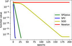
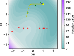
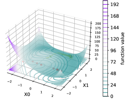
Figure 1: The PermD$\beta^{+}$ function with $\beta=0.5$ where Left: we plot $f(x)$ across epochs Middle: level set plot, Right: Surface plot. SP2 is in blue , SP2⁺ is in green , SGD is in yellow and Newton in red.

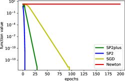
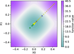
Figure 2: The Rastrigin function where Left: we plot $f(x)$ across epochs Middle: level set plot, Right: Surface plot. SP2 is in blue , SP2⁺ is in green , SGD is in yellow and Newton is in red.

6.2 Matrix Completion

Assume a set of known values $\{a_{i,j}\}_{(i,j)\in\Omega}$ where $\Omega$ is a set of known elements of the matrix, and we want to determine the missing elements. One approach is solving the matrix completion problem

$$\min_{U,V}\sum_{(i,j)\in\Omega}\frac{1}{2}(u_{i}^{T}v_{j}-a_{i,j})^{2},$$ (32)

where $U=[u_{i}]_{(i,j)\in\Omega}$ and $V=[v_{j}]_{(i,j)\in\Omega}$. With the solution to (32), we then use $U^{\top}V$ as an approximation to the complete matrix $A=[a_{i,j}]_{i,j=1,\ldots,n}.$

Depite (32) being a non-convex problem, if there exists an interpolating solution to (32), that is one where $u_{i}^{T}v_{j}=a_{i,j},~{}\mbox{for }(i,j)\in\Omega$, then the SP2 method can solve (32). Indeed, the SP2 can be applied to (32) by sampling a single pair $(i,j)\in\Omega$ uniformly, then projecting onto the quadratic

$$u_{i}^{k+1},v_{j}^{k+1} =\;\operatorname{argmin}_{u,v}\frac{1}{2}\left\|u-u_{i}^{k}\right\|^{2}+\frac{1}{2}\left\|v-v_{j}^{k}\right\|^{2}\mbox{ subject to }u^{\top}v=a_{i,j}.$$ (33)

This projection can be solved as we detail in Theorem B.1 in Appendix B.

We compared our method 33 to a specialized variant of SGD for online matrix completion described in [19], see Figure 3. To compare the two methods we generated a rank $k=2$ matrix $A\in\mathbb{R}^{100\times 50}$. We selected a subset entries with probability $p=0.1,0.2$ or $0.3$ to form our set $\Omega_{init}$ that was used to obtain an initial estimate $U_{0},V_{0}$ using rank-k SVD method as described in [19]. We extensively tuned the step size of SGD using a grid search, and the method labelled Non-convex SGD is the resulting run of SGD with the best step size. We also show how sensitive SGD is to this step size, by including the run of SGD with step sizes that were only a factor of $2$ to $4$ away from the optimal, which greatly degrades the performance of SGD. In contrast, SP2 worked with no tuning, and matches the performance of SGD with the optimal step size in the $p=0.1$ experiment, and outperforms SGD in the experiments with more measurements as can be seen in the $p=0.2$ and $p=0.3$ figures.

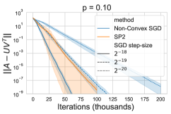
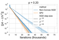
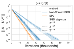
Figure 3: Recovery error for matrix completion. Left: Using 10%, Middle: using 20% and Right: using 30% of the entries of $A$ to form $\Omega$, respectively. Shaded region corresponds to $5$ repeated runs.

6.3 Convex classification

In this experiment, we test the proposed methods on a logistic regression problem and compare them with some state-of-the-art methods (e.g., SGD, SP, and ADAM). In particular, we consider the problem of minimizing the following loss function $f(w)=\frac{1}{n}\sum_{i=1}^{n}f_{i}(w)+\frac{\sigma}{2}\|w\|_{2}^{2},$ where $f_{i}(w)=\phi_{i}(x_{i}^{\top}w)$ with $\phi_{i}(t)=\ln(1+e^{-y_{i}t})$. Here, $\{(x_{i},y_{i})\in\mathbb{R}^{d+1}\}_{i=1}^{n}$ stands for the feature-label pairs and $\sigma>0$ is the regularization parameter. We can control how far each problem is from interpolation by increasing $\sigma$. When $\sigma>0$ the problem cannot interpolate, and thus we expect to see a benefit of the slack methods in Section 5 over SP2⁺.

We used two data sets: colon-cancer [2] and mushrooms [37], both of which interpolate when $\sigma=0.$

We compare the proposed methods SP2⁺ (20), SP2L2⁺ (Lemma C.5), SP2L1⁺ (Lemma C.7), and SP2max⁺ (Lemma C.8) with SGD, SP (5), and ADAM on both data sets with three regularizations $\sigma\in\{0,\;0.001,\;0.008\}$ and with momentum set to $0.3$. For the SGD method, we use a learning rate $L_{\max}/\sqrt{t}$ in the $t$-th iteration, where $L_{\max}=\frac{1}{4}\max_{i=1,\ldots,n}\|x_{i}\|^{2}$ denotes the smoothness constant of the loss function. We chose $\lambda$ for SP2L2⁺, SP2L1⁺, and SP2max⁺ using a grid search of $\lambda\in\{0.1,0.2,\ldots,0.9\}$, the details are in Section D.

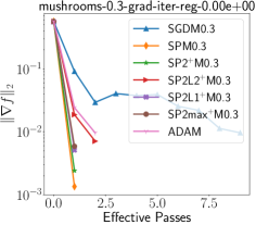
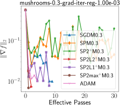
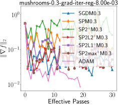
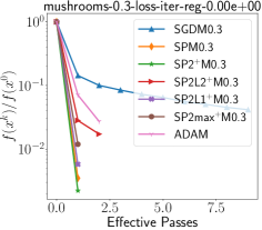
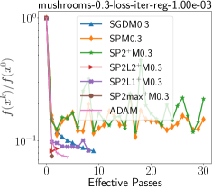
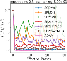
Figure 13: Mushrooms: gradient norm and loss at each epoch with momentum being $0.3$.

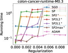
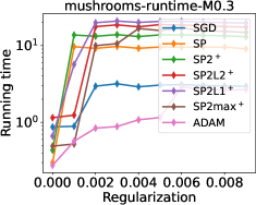
Figure 14: Running time in seconds.

The gradient norm and loss evaluated at each epoch are presented in Figures 4 and 13 (see Appendix D). We see that SP2 methods converge much faster than classical methods (e.g., SGD, SP, ADAM) and need fewer epochs to achieve the tolerance when $\sigma$ is small (left and middle plots). However, they can all fail when the problem is far from interpolation, e.g., when $\sigma=8\times 10^{-3}$. The running time used for each algorithm to achieve either the tolerance or maximum number of epochs for both data sets is presented in Figure 14 (see Appendix D).

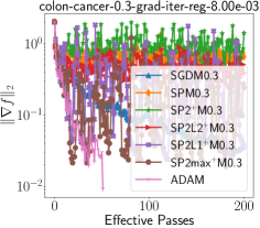
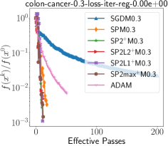
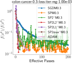
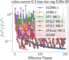
Figure 4: Colon-cancer: gradient norm and loss at each epoch with momentum being $0.3$. Left: $\sigma=0,$ Middle: $\sigma=0.001$ and Right $\sigma=0.008$.

7 Conclusion

Here we have proposed new incremental second order methods that exploit models that interpolate the data, or are close to interpolation. What sets our methods apart from most previous incremental second order methods is that they do not rely on convexity in their design. Quite the opposite, the SP2 method can benefit from the Hessian having at least one negative eigenvalue. Consequently the SP2 method excels at minimizing non-convex models that interpolate, as can be seen in Sections 6.1 and B. We also provided an indicative convergence in Theorem C.1 that shows that SP2 and its approximation SP2⁺ enjoy a significantly faster rate of convergence as compared to SGD for sums-of-quadratics.

We then developed second order methods that can solve a relaxed version of the interpolation equations that allows for some slack in Section 5, and showed that these methods still perform well on problems that are close to interpolation in Section 6.3.

In future work, it would be interesting to develop specialized variants of SP2 for optimizing (DNNs) Deep Neural Networks. DNNs are particularly well suited since they can interpolate, are non-convex and since gradients and Hessian vector products can be computed efficiently using back-propagation.

Appendix A Appendix

A.1 Projecting onto Quadratic

This following projection lemma is based on Section B in [28]. What we do in addition to [28] is to clarify how to compute the resulting projection, and add further details on the proof.

Lemma A.1.

Let $w\in\mathbb{R}^{d}$ and let ${\bf P}\in\mathbb{R}^{d\times d}$ is a symmetric matrix. Consider the projection

$$w^{\prime}\in \operatorname{argmin}_{w\in\mathbb{R}^{d}}\tfrac{1}{2}\left\|w-z\right\|^{2}$$

$$\mbox{ s.t. }r+\left<q,w-z\right>+\tfrac{1}{2}\left<{\bf P}(w-z),w-z\right>=0.$$ (34)

Let

$$\lambda_{1}\leq\lambda_{2}\leq\cdots\leq\lambda_{d}$$

be the eigenvalues of ${\bf P}$ and let $Q\Lambda Q^{\top}={\bf P}$ be the eigenvalue decomposition of ${\bf P}$, where $\Lambda=\mbox{diag}(\lambda_{i})$ and $QQ^{\top}=I.$ Let $\hat{q}=Q^{\top}q$. If the quadratic constraint in (34) is feasible, then there exists a solution to (34). Now we give the three candidate solutions.

1. If $r=0$, then the solution is given by

   $$w=z.$$

2. Now assuming $r\neq 0.$ Let

   $$\nu = \max_{i\;:\;\lambda_{i}\neq 0}\left\{-\frac{1}{\lambda_{1}},-\frac{1}{\lambda_{d}}\right\}$$ (35)

   $$i^{*} \in \arg\max_{i\;:\;\lambda_{i}\neq 0}\left\{-\frac{1}{\lambda_{1}},-\frac{1}{\lambda_{d}}\right\}$$ (36)

   $$N = \{i\;:\;\lambda_{i}\neq\lambda_{i^{*}}\}.$$ (37)

   Let

   $$x^{*} = -({\bf I}+\nu\Lambda)^{\dagger}\nu\hat{q}.$$ (38)

   If

   $$2\nu r+\nu\left<\hat{q},x^{*}\right>-\left\|x^{*}\right\|^{2}+\frac{\nu^{2}}{4}\sum_{i\in N}\hat{q}_{i}^{2}\geq 0$$ (39)

   then the solution is given by

   $$w^{\prime}=z+Q(x^{*}+n),$$ (40)

   where $n\in\mathbb{R}^{d}$ and

   $$n_{i} =\frac{\nu}{2}\hat{q}_{i}+\frac{1}{\sqrt{|N|}}\sqrt{2\nu r+\nu\left<\hat{q},x^{*}\right>-\left\|x^{*}\right\|^{2}+\frac{\nu^{2}}{4}\sum_{i\in N}\hat{q}_{i}^{2}},\quad\mbox{for }i\in N$$

   $$n_{i} =0,\quad\mbox{for }i\not\in N.$$

3. Alternatively if (39) does not hold, then the solution is given by

   $$w^{\prime} = z-({\bf I}+\nu\Lambda)^{\dagger}\nu q$$ (41)

   where $\nu$ is the solution to the nonlinear equation

   $$\frac{\nu}{2}\sum_{i}\frac{\hat{q}_{i}^{2}(2+\nu\lambda_{i})}{(1+\nu\lambda_{i})^{2}} = r.$$ (42)

Proof.

First note that there exists a solution to (34) since the constraint is a closed feasible set.

Let $Q\Lambda Q^{\top}={\bf P}$ be the SVD of ${\bf P}$, where $QQ^{\top}=I.$ By changing variables $x=Q^{\top}(w-z)$ we have that (34) is equivalent to

$$\operatorname{argmin}_{\hat{x}\in\mathbb{R}^{d}}\tfrac{1}{2}\left\|x\right\|^{2}$$

$$\mbox{ s.t. }r+\left<\hat{q},x\right>+\tfrac{1}{2}\left<\Lambda x,x\right>=0,$$ (43)

where $\hat{x}=Q^{\top}(w-z)$ and $\hat{q}=Q^{\top}q.$ The Lagrangian of (43) is given by

$$L(x,\nu) =\;\tfrac{1}{2}\left\|x\right\|^{2}+\nu\big{(}r+\left<\hat{q},x\right>+\tfrac{1}{2}\left<\Lambda x,x\right>\big{)}$$

$$=\;\tfrac{1}{2}x^{\top}({\bf I}+\nu\Lambda)x+\nu\big{(}r+\left<\hat{q},x\right>\big{)}.$$ (44)

Thus the KKT conditions are given by

$$\nabla_{x}L(x,\nu) =({\bf I}+\nu\Lambda)x+\nu\hat{q}=0$$ (45)

$$\nabla_{\nu}L(x,\nu) =r+\left<\hat{q},x\right>+\tfrac{1}{2}\left<\Lambda x,x\right>=0.$$ (46)

Since we are guaranteed that the projection has a solution, we have that as a necessary condition that the solution satisfies

$$\nabla_{x}^{2}L(x,\nu)=({\bf I}+\nu\Lambda)\succeq 0,$$

see Theorem 12.5 in [38]. Consequently either $({\bf I}+\nu\Lambda)\succ 0$ or $({\bf I}+\nu\Lambda)$ has a zero eigenvalue.

Consider the case where $({\bf I}+\nu\Lambda)\succ 0.$ From (45) we have that

$$x=-\nu({\bf I}+\nu\Lambda)^{-1}\hat{q}.$$ (47)

Now note that if $\nu=0$ then $x=0$ and by the constraint we must have $r=0$. Otherwise, if $r\neq 0,$ then $\nu\neq 0.$ Assume now $\nu\neq 0$ and substituting the above into (46) and letting $\Lambda=\mbox{diag}(\lambda_{i})$ gives

$$\nabla_{\nu}L(x,\nu) =r+\left<\hat{q},x\right>+\tfrac{1}{2\nu}\left<\nu\Lambda x,x\right>$$

$$=r+\left<\hat{q},x\right>+\tfrac{1}{2\nu}\left<({\bf I}+\nu\Lambda)x,x\right>-\frac{1}{2\nu}\left\|x\right\|^{2}$$

$$=r+\frac{1}{2}\left<\hat{q},x\right>-\frac{1}{2\nu}\left\|x\right\|^{2}$$ Using (45)

$$=r-\frac{\nu}{2}\left<\hat{q},({\bf I}+\nu\Lambda)^{-1}\hat{q}\right>-\frac{\nu}{2}\left\|({\bf I}+\nu\Lambda)^{-1}\hat{q}\right\|^{2}$$ Using (47)

$$=r-\frac{\nu}{2}\sum_{i}\left(\frac{\hat{q}_{i}^{2}}{1+\nu\lambda_{i}}+\frac{\hat{q}_{i}^{2}}{(1+\nu\lambda_{i})^{2}}\right).$$

Thus

$$\frac{\nu}{2}\sum_{i}\frac{\hat{q}_{i}^{2}(2+\nu\lambda_{i})}{(1+\nu\lambda_{i})^{2}} = r.$$ (48)

Upon finding the solution $\nu$ to the above, we have that our final solution is given by $w^{\prime}=z+Qx,$ that is

$$w^{\prime} = z-Q({\bf I}+\nu\Lambda)^{\dagger}\nu\hat{q}$$ (49)

$$= z-({\bf I}+\nu\Lambda)^{\dagger}\nu Q\hat{q}$$

$$= z-\nu({\bf I}+\nu\Lambda)^{\dagger}q$$

Alternatively, suppose that $({\bf I}+\nu\Lambda)\succeq 0$ is non-singular. The positive definiteness implies that

$$\nu\;\geq\;-\frac{1}{\lambda_{i}},\quad\mbox{for }i=1,\ldots,d.$$ (50)

For $({\bf I}+\nu\Lambda)$ to be non-singular, at least one of the above inequalities will hold to equality. To ease notation, let us arrange the eigenvalues in increasing order so that

$$\lambda_{1}\leq\lambda_{2}\leq\cdots\leq\lambda_{d}.$$

For one of the (50) inequalities to hold to equality we need that

$$\nu\;=\;\max_{i\;:\;\lambda_{i}\neq 0}-\frac{1}{\lambda_{i}}=\max_{i\;:\;\lambda_{i}\neq 0}\left\{-\frac{1}{\lambda_{1}},-\frac{1}{\lambda_{d}}\right\}.$$

Since $({\bf I}+\nu\Lambda)$ is now singular with this $\nu$, we have that the solution to (45) is given by

$$x\;=\;-({\bf I}+\nu\Lambda)^{\dagger}\nu\hat{q}+n\;\coloneqq\;x^{*}+n,\quad\mbox{where }\left<x^{*},n\right>=0,$$ (51)

where $\dagger$ denotes the pseudo-inverse and where $n$ is in the kernel of $({\bf I}+\nu\Lambda)$, in other words $({\bf I}+\nu\Lambda)n=0.$ It remains to determine $n$, which we can do with (46). Indeed, substituting (51) into (46) gives

$$\nabla_{\nu}L(x,\nu) =r+\frac{1}{2}\left<\hat{q},x\right>-\frac{1}{2\nu}\left\|x\right\|^{2}$$ Using (45)

$$=r+\frac{1}{2}\left<\hat{q},x^{*}+n\right>-\frac{1}{2\nu}\left\|n\right\|^{2}-\frac{1}{2\nu}\left\|x^{*}\right\|^{2}. \mbox{Using~{}\eqref{eq:tempnxo848os}}.$$

Setting to zero and completing the squares in $n$ we have that

$$\frac{1}{2\nu}\left\|n-\frac{\nu}{2}\hat{q}\right\|^{2}=r+\frac{1}{2}\left<\hat{q},x^{*}\right>-\frac{1}{2\nu}\left\|x^{*}\right\|^{2}+\frac{\nu}{8}\left\|\hat{q}\right\|^{2}.$$ (52)

To characterize the solutions in $n$ of the above, first note that $n$ will only have a few non-zero elements. To see this, let $i^{*}\in\arg\max_{i\;:\;\lambda_{i}\neq 0}\left\{-\frac{1}{\lambda_{1}},-\frac{1}{\lambda_{d}}\right\}$, and note that $({\bf I}+\nu\Lambda)$ has as many zeros on the diagonal as the multiplicity of the eigenvalue $\lambda_{i^{*}}.$ That is, it has zeros elements on the indices in

$$I\;=\;\{i\;:\;\lambda_{i}=\lambda_{i^{*}}\}.$$

Thus the non-zero elements of $n$ are in the set

$$N\;=\;\{i\;:\;\lambda_{i}\neq\lambda_{i^{*}}\}.$$

Because of this observation we further re-write (52) as

$$\sum_{i\in N}\left(n_{i}-\frac{\nu}{2}\hat{q}_{i}\right)^{2} = 2\nu r+\nu\left<\hat{q},x^{*}\right>-\left\|x^{*}\right\|^{2}+\frac{\nu^{2}}{4}\left\|\hat{q}\right\|^{2}-\sum_{i\in I}\frac{\nu^{2}}{4}\hat{q}^{2}_{i}$$ (53)

$$= 2\nu r+\nu\left<\hat{q},x^{*}\right>-\left\|x^{*}\right\|^{2}+\frac{\nu^{2}}{4}\sum_{i\in N}\hat{q}_{i}^{2}.$$

Consequently, if the above is positive, then there exists solutions to the above of which

$$n_{i}=\frac{\nu}{2}\hat{q}_{i}+\frac{1}{\sqrt{|N|}}\sqrt{2\nu r+\nu\left<\hat{q},x^{*}\right>-\left\|x^{*}\right\|^{2}+\frac{\nu^{2}}{4}\sum_{i\in N}\hat{q}_{i}^{2}},\quad\mbox{for }i\in N.$$ (54)

is one. Consequently, the final solution is given by $w=z+Q(x^{*}+n)$ where $x^{*}$ is given in by (51). ∎

Corollary A.2.

If $r>0$ and ${\bf P}$ has at least one negative eigenvalue, there always exists a solution to the projection (34).

Proof.

We only need to prove that there exists a solution to the quadratic equation in (34), after which Lemma A.1 guarantees the existance of a solution. ∎

Appendix B Matrix Completion

The projection (33) can be solved as we shown in the following theorem.

Theorem B.1.

The solution to  (33) is given by one of the following cases.

1. If $(u_{j}^{k})^{\top}v_{j}^{k}=a_{i,j}$ then $u=u^{k}_{i}$ and $v=v^{k}_{j}.$

2. Alternatively if $u_{j}^{k}=v_{j}^{k}$ and

   $$(u_{j}^{k})^{\top}v_{j}^{k}\geq 4a_{i,j}$$

   then

   $$v =\frac{1}{2}v_{j}^{k}+\frac{1}{2}\frac{v_{j}^{k}}{\left\|v_{j}^{k}\right\|}\sqrt{\left\|v_{j}^{k}\right\|^{2}-4a_{i,j}}$$ (55)

   $$u =-\frac{1}{2}u_{j}^{k}+\frac{1}{2}\frac{u_{j}^{k}}{\left\|u_{j}^{k}\right\|}\sqrt{\left\|u_{j}^{k}\right\|^{2}-4a_{i,j}}$$ (56)

3. Finally, if none of the above holds then

   $$u =\frac{u_{i}^{k}-\gamma v_{j}^{k}}{1-\gamma^{2}}$$ (57)

   $$v =\frac{v_{j}^{k}-\gamma u_{i}^{k}}{1-\gamma^{2}},$$ (58)

   where $\gamma\in(-1,1)$ and is the solution to the depressed quartic equation

   $$(1+\gamma^{2})\left<u_{i}^{k},v_{j}^{k}\right>-\gamma(\left\|u_{i}^{k}\right\|^{2}+\left\|v_{j}^{k}\right\|^{2}) =(1-\gamma^{2})^{2}a_{i,j}.$$ (59)

Proof.

The Lagrangian of (33) is given by

$$L(u,v,\gamma)\;=\;\tfrac{1}{2}\left\|u-u_{i}^{k}\right\|^{2}+\tfrac{1}{2}\left\|v-v_{j}^{k}\right\|^{2}+\gamma(u^{\top}v-a_{i,j}),$$

where $\gamma\in\mathbb{R}$ is the unknown Lagrangian Multiplier. Thus the KKT equations are

$$u-u_{i}^{k}+\gamma v =0$$ (60)

$$v-v_{j}^{k}+\gamma u =0$$ (61)

$$u^{\top}v =a_{i,j}$$ (62)

Subtracting $\gamma$ times the the second equation from the first equation, and analogously, subtracting the first equation from the second gives

$$(1-\gamma^{2})u-u_{i}^{k}+\gamma v_{j}^{k} =0$$ (63)

$$(1-\gamma^{2})v-v_{j}^{k}+\gamma u_{i}^{k} =0.$$ (64)

If $\gamma=1$, then necessarily $u^{k}_{i}=v_{j}^{k}$ and furthermore from the first equation in (62) we have that

$$u=u_{i}^{k}-v=v_{j}^{k}-v.$$ (65)

Substituting $u$ out in the original projection problem (33) we have that

$$\;\min_{v}\left\|v\right\|^{2}-v^{\top}v_{j}^{k}\;\mbox{ subject to }\;v^{\top}v_{j}^{k}-\left\|v\right\|^{2}=a_{i,j}.$$ (66)

Consequently, for every $v$ that satisfies the constraint we have that the objective value is invariant and equal to $-a_{i,j}.$ Consequently there are infinite solutions. To find one such solution, we complete the squares of the constraint and find

$$\left\|v-\tfrac{1}{2}v_{j}^{k}\right\|^{2} = \frac{1}{4}\left\|v_{j}^{k}\right\|^{2}-a_{i,j}.$$ (67)

The above only has solutions if $\frac{1}{4}\left\|v_{j}^{k}\right\|^{2}-a_{i,j}\geq 0.$ One solution to the above is given by (55).

Alternatively, if $\gamma\neq 1$ then by isolating $u$ and $v$ in (63) and (64), respectively, gives

$$u =\frac{u_{i}^{k}-\gamma v_{j}^{k}}{1-\gamma^{2}}$$ (68)

$$v =\frac{v_{j}^{k}-\gamma u_{i}^{k}}{1-\gamma^{2}}$$ (69)

To figure out $\gamma$, we use the third constraint in (62) and the above two equations, which gives

$$u^{\top}v =\frac{(u_{i}^{k}-\gamma v_{j}^{k})^{\top}}{1-\gamma^{2}}\frac{v_{j}^{k}-\gamma u_{i}^{k}}{1-\gamma^{2}}$$

$$=\frac{(1+\gamma^{2})\left<u_{i}^{k},v_{j}^{k}\right>-\gamma(\left\|u_{i}^{k}\right\|^{2}+\left\|v_{j}^{k}\right\|^{2})}{(1-\gamma^{2})^{2}}\;=\;a_{i,j}.$$

Let

$$\phi(\gamma)=(1+\gamma^{2})\left<u_{i}^{k},v_{j}^{k}\right>-\gamma(\left\|u_{i}^{k}\right\|^{2}+\left\|v_{j}^{k}\right\|^{2})-(1-\gamma^{2})^{2}a_{i,j}.$$

Can we now find an interval which will contain the solution in $\gamma$? Note that

$$\phi(-1) =2\left<u_{i}^{k},v_{j}^{k}\right>+\left\|u_{i}^{k}\right\|^{2}+\left\|v_{j}^{k}\right\|^{2}=\left\|u_{i}^{k}+v_{j}^{k}\right\|^{2}\geq 0$$

$$\phi(1) =2\left<u_{i}^{k},v_{j}^{k}\right>-\left\|u_{i}^{k}\right\|^{2}-\left\|v_{j}^{k}\right\|^{2}=-\left\|u_{i}^{k}-v_{j}^{k}\right\|^{2}\leq 0.$$

Thus it suffices to search for $\gamma\in(-1,\;1),$ which can be done efficiently with bisection.

∎

Appendix C Proofs of Important Lemmas

C.1 Proof of Lemma 3.1

Let us first describe the set of solutions for given constraint. We need to have

$$f_{i}+a_{i}x_{i}^{T}\Delta+\frac{1}{2}h_{i}\Delta^{T}x_{i}x_{i}^{T}\Delta=0,$$ (70)

where $\Delta=w-w^{t}$ is unknown. If we denote by $\tau_{i}=x_{i}^{T}\Delta$ then (70) will reduce to

$$f_{i}+a_{i}\tau_{i}+\frac{1}{2}h_{i}\tau_{i}^{2}=0.$$ (71)

This quadratic equation  (71) has solution if

$$a_{i}^{2}-2h_{i}f_{i}\geq 0.$$ (72)

If the condition above holds then we have that the solution for $\tau$ is in this set

$$T^{*}:=\left\{\frac{-a_{i}+\sqrt{a_{i}^{2}-2h_{i}f_{i}}}{h_{i}},\frac{-a_{i}-\sqrt{a_{i}^{2}-2h_{i}f_{i}}}{h_{i}}\right\}.$$ (73)

Recall that the problem (7) now reduces into

$$\min_{\Delta}\left\{\|\Delta\|^{2},\ \mbox{such that}\ x_{i}^{T}\Delta\in T^{*}\right\}.$$ (74)

Note that because we want to minimize $\|\Delta\|^{2}$, we want to choose the constraint with smallest possible absolute value, hence the problem (74) is equivalent to

$$\min_{\Delta}\left\{\|\Delta\|^{2},\ \mbox{such that}\ x_{i}^{T}\Delta=\tau_{i}^{*}\right\},$$ (75)

where

$$\tau_{i}^{*}=\begin{cases}\frac{-a_{i}+\sqrt{a_{i}^{2}-2h_{i}f_{i}}}{h_{i}},&\mbox{if}\ a_{i}>0\\ \frac{-a_{i}-\sqrt{a_{i}^{2}-2h_{i}f_{i}}}{h_{i}},&\mbox{otherwise}.\end{cases}$$

In other words,

$$\tau_{i}^{*}=-\frac{a_{i}}{h_{i}}+\mbox{sign}(a_{i})\frac{\sqrt{a_{i}^{2}-2h_{i}f_{i}}}{h_{i}}=\frac{a_{i}}{h_{i}}\left(\frac{\sqrt{a_{i}^{2}-2h_{i}f_{i}}}{|a_{i}|}-1\right)$$

The final solution is hence

$$\Delta^{*}=\frac{\tau_{i}^{*}}{\|x_{i}\|^{2}}x_{i}$$

and therefore

$$w^{*}=w^{t}+\frac{\tau_{i}^{*}}{\|x_{i}\|^{2}}x_{i}$$

In case when (72) is not satisfied, and because we assumed that the loss function is non-negative, we necessary have $h_{i}>0$. Then natural choice of $\tau_{i}$ is the one that would minimize the

$$f_{i}+a_{i}\tau_{i}+\frac{1}{2}h_{i}\tau_{i}^{2}.$$

From first order optimality conditions we obtain that

$$\tau_{i}^{*}=-\frac{a_{i}}{h_{i}}$$

which leads to (14).

C.2 Proof of Lemma 3.2

Proof.

If $\phi(t)=0$ then the condition holds trivially. For $t$ such that $\phi(t)\neq 0$, $\sqrt{\phi(t)}$ is differentiable, and we have

$$\frac{d^{2}}{dt^{2}}\sqrt{\phi(t)} =-\tfrac{1}{4}\phi(t)^{-3/2}\phi^{\prime}(t)^{2}+\tfrac{1}{2}\phi(t)^{-1/2}\phi^{\prime\prime}(t)=\tfrac{1}{4}\phi(t)^{-3/2}(-\phi^{\prime}(t)^{2}+2\phi(t)\phi^{\prime\prime}(t)),$$

which is negative precisely when $\phi^{\prime}(t)^{2}\geq 2\phi(t)\phi^{\prime\prime}(t).$ ∎

C.3 Proof of Lemma 3.3

Note that

$$q(w^{t+1/2}) \overset{\eqref{eq:polyakup}+\eqref{eq:quadeqzero2}}{=}f_{i}(w^{t})-\left<\nabla f_{i}(w^{t}),\frac{f_{i}(w^{t})}{\left\|\nabla f_{i}(w^{t})\right\|^{2}}\nabla f_{i}(w^{t})\right>$$

$$\quad\quad+\frac{1}{2}\left<\nabla^{2}f_{i}(w^{t})\frac{f_{i}(w^{t})}{\left\|\nabla f_{i}(w^{t})\right\|^{2}}\nabla f_{i}(w^{t}),\frac{f_{i}(w^{t})}{\left\|\nabla f_{i}(w^{t})\right\|^{2}}\nabla f_{i}(w^{t})\right>$$

$$\quad=\frac{1}{2}\frac{f_{i}(w^{t})^{2}}{\left\|\nabla f_{i}(w^{t})\right\|^{4}}\left<\nabla^{2}f_{i}(w^{t})\nabla f_{i}(w^{t}),\nabla f_{i}(w^{t})\right>.$$

Furthermore

$$\nabla q(w^{t+1/2}) \overset{\eqref{eq:quadeqzero2}}{=} \nabla f_{i}(w^{t})+\nabla^{2}f_{i}(w^{t})(w^{t+1/2}-w^{t})$$

$$\overset{\eqref{eq:polyakup}}{=} \left({\bf I}-\nabla^{2}f_{i}(w^{t})\frac{f_{i}(w^{t})}{\left\|\nabla f_{i}(w^{t})\right\|^{2}}\right)\nabla f_{i}(w^{t}).$$

Thus the second step (19) is given by

$$w^{t+1}=w^{t+1/2}-\frac{1}{2}\frac{f_{i}(w^{t})^{2}}{\left\|\nabla f_{i}(w^{t})\right\|^{4}}\frac{\left<\nabla^{2}f_{i}(w^{t})\nabla f_{i}(w^{t}),\nabla f_{i}(w^{t})\right>}{\left\|\left({\bf I}-\nabla^{2}f_{i}(w^{t})\frac{f_{i}(w^{t})}{\left\|\nabla f_{i}(w^{t})\right\|^{2}}\right)\nabla f_{i}(w^{t})\right\|^{2}}\cdot\left({\bf I}-\nabla^{2}f_{i}(w^{t})\frac{f_{i}(w^{t})}{\left\|\nabla f_{i}(w^{t})\right\|^{2}}\right)\nabla f_{i}(w^{t}).$$ (76)

Putting the first (17) and second (76) updates together gives (20).

This gives a second order correction of the Polyak step that only requires computing a single Hessian-vector product that can be done efficiently using an additional backwards pass of the function. We call this method SP2.

C.4 Convergence of multi-step SP2⁺

If we apply multiple steps of the SP2⁺, as opposed to two steps, the method converges to the solution of (15). This follows because each step of SP2⁺ is a step of NR Newton Raphson’s method applied to solving the nonlinear equation

$$q(w)\coloneqq f_{i}(w^{t})+\left<\nabla f_{i}(w^{t}),w-w^{t}\right>+\tfrac{1}{2}\left<\nabla^{2}f_{i}(w^{t})(w-w^{t}),w-w^{t}\right>.$$

Indeed, starting from $w^{0}=w^{t}$, the iterates of the NR (Newton Raphson) method are given by

$$w^{i+1}=w^{i}-\left(\nabla q(w^{i})^{\top}\right)^{\dagger}q(w^{i})=w^{i}-\frac{q(w^{i})}{\left\|\nabla q(w^{i})\right\|^{2}}\nabla q(w^{i}),$$ (77)

where ${\bf M}^{\dagger}$ denotes the pseudo-inverse of the matrix ${\bf M}.$

The NR iterates in (77) can also be written in a variational form given by

$$w^{i+1}= \operatorname{argmin}_{w\in\mathbb{R}^{d}}\left\|w-w^{i}\right\|^{2}$$

$$\mbox{ s.t. }q(w^{i})+\nabla q(w^{i})(w-w^{i})=0.$$ (78)

Comparing the above to the first (16) and second step (18) are indeed two steps of the NR method. Further, we can see that (C.4) is indeed the multi-step version of SP2⁺.

This method (77) is also known as gradient descent with a Polyak Step step size, or SP for short. It is this connection we will use to prove the convergence of (77) to a root of $q(w).$

We assume that $q(w)$ has at least one root. Let $w_{q}^{*}\in\mathbb{R}^{d}$ be a least norm root of $q(w),$ that is

$$w_{q}^{*} =\operatorname{argmin}\left\|w\right\|^{2}\quad\mbox{subject to }\;q(w)=0.$$ (79)

It follows from Theorem 3.2 of [34] that the above optimization (79) has solution if and only if the following matrix

$$B =(\nabla f_{i}(w^{t})-\nabla^{2}f_{i}(w^{t})w^{t})(\nabla f_{i}(w^{t})-\nabla^{2}f_{i}(w^{t})w^{t})^{\top}+$$

$$\qquad 2\left(-f_{i}(w^{t})+\nabla f_{i}(w^{t})^{\top}w^{t}-\frac{1}{2}{w^{t}}^{\top}\nabla^{2}f_{i}(w^{t})w^{t}\right)\nabla^{2}f_{i}(w^{t})$$ (80)

has at least a non-negative eigenvalue.

Theorem C.1.

Assume that the matrix $B$ defined in (80) has at least a non-negative eigenvalue. If $q(w)$ is star-convex with respect to $w_{q}^{*}$, that is if

$$(w^{i}-w_{q}^{*})^{\top}\nabla^{2}f_{i}(w^{t})(w^{i}-w_{q}^{*})\geq 0,\quad\mbox{for all }i,$$ (81)

then it follows that

$$\min_{i=0,\ldots,T-1}q(x^{i})\;\leq\;\frac{\sigma_{\max}(\nabla^{2}f_{i}(w^{t}))}{2T}\left\|w^{0}-w_{q}^{*}\right\|^{2}.$$ (82)

Proof.

The proof follows by applying the convergence Theorem 4.4 in [15] or equivalently Corollary D.3 in [13]. This result first appeared in Theorem 4.4 in [15], but we apply Corollary D.3 in [13] since it is a bit simpler.

To apply this Corollary D.3 in [13], we need to verify that $q$ is an $L$–smooth function and star-convex. To verify if it is smooth, we need to find $L>0$ such that

$$q(w)\;\leq\;q(y)+\left<\nabla q(y),w-y\right>+\frac{L}{2}\left\|w-y\right\|^{2},$$ (83)

which holds with $L=\sigma_{\max}(\nabla^{2}q(y))=\sigma_{\max}(\nabla^{2}f_{i}(w^{t})$ since $q$ is a quadratic function. Furthermore, for $q$ to be star-convex along the iterates $w^{i}$, we need to verify if

$$q(w^{*}_{q})\;\geq\;q(w^{i})+\left<\nabla q(w^{i}),w^{*}-w^{i}\right>.$$ (84)

Since $q$ is a quadratic, we have that

$$q(w^{*}_{q})=q(w^{i})+\left<\nabla q(w^{i}),w^{*}-w^{i}\right>+\left<\nabla^{2}q(w^{i})(w^{*}-w^{i}),w^{*}-w^{i}\right>.$$

Using this in (85) gives that

$$0\;\geq\;\left<\nabla^{2}q(w^{i})(w^{*}-w^{i}),w^{*}-w^{i}\right>=\left<\nabla^{2}f_{i}(w^{t})(w^{*}-w^{i}),w^{*}-w^{i}\right>,$$ (85)

which is equivalent to our assumption (81). We can now apply the result in Corollary D.3 in [13] which states that

$$\min_{i=0,\ldots,T-1}(q(x^{i})-q(w_{q}^{*}))\;\leq\;\frac{L}{2T}\left\|w^{0}-w_{q}^{*}\right\|^{2}.$$

Finally using $q(w_{q}^{*})=0$ and that $L=\sigma_{\max}(\nabla^{2}f_{i}(w^{t}))$ gives the result. ∎

To simplify notation, we will omit the dependency on $w^{t}$ and denote $c=f_{i}(w^{t})$, $g=\nabla f_{i}(w^{t})$ and ${\bf H}=\nabla^{2}f_{i}(w^{t}),$ thus

$$q(w) =c+\left<g,w-w^{t}\right>+\frac{1}{2}\left<{\bf H}(w-w^{t}),w-w^{t}\right>$$

$$\nabla q(w) =g+{\bf H}(w-w^{t})$$

$$\nabla^{2}q(w) ={\bf H}$$ (86)

Lemma C.2.

If $g\in\operatorname{Range}({\bf H})$ and $w^{0}\in\operatorname{Range}({\bf H})$ then $w^{i},\nabla q(w^{i})\in\operatorname{Range}({\bf H})$ for all $i$ and $w_{q}^{*}\in\operatorname{Range}({\bf H})$.

Proof.

First, note that since $g\in\operatorname{Range}({\bf H})$ and since $\nabla q(w)=q+{\bf H}(w-w^{t})$ (see (86)) we have that $\nabla q(w)\in\operatorname{Range}({\bf H})$ for all $w$. Consequently by induction if $w^{i}\in\operatorname{Range}({\bf H})$ then by (77) we have that $w^{i+1}\in\operatorname{Range}({\bf H})$ since it is a combination of $\nabla q(w^{i})$ and $w^{i}$.

Finally, let $w_{q}^{*}=w^{t}+w_{{\bf H}}+w_{{\bf H}}^{\perp}$ where $w_{{\bf H}}\in\operatorname{Range}({\bf H})$ and $w_{{\bf H}}^{\perp}\in\operatorname{Range}({\bf H})^{\perp}.$ It follows that

$$q(w_{q}^{*})=q(w^{t}+w_{{\bf H}}).$$

Furthermore, by orthogonality and Pythagoras’ Theorem

$$\left\|w_{q}^{*}\right\|=\left\|w^{t}+w_{{\bf H}}\right\|+\left\|w_{{\bf H}}^{\perp}\right\|$$

Consequently, since $w_{q}^{*}$ is the least norm solution, we must have that $w_{{\bf H}}^{\perp}=0$ and thus $w_{q}^{*}\in\operatorname{Range}({\bf H}).$ ∎

C.5 Proof of Proposition 4.1

First we repeat the proposition for ease of reference.

Proposition C.3.

Consider the loss functions given in (21). The SP2 method converges (7) converges according to

$$\mathbb{E}\left[\left\|w^{t+1}-w^{*}\right\|^{2}\right]\leq\rho\;\mathbb{E}\left[\left\|w^{t}-w^{*}\right\|^{2}\right],$$ (87)

where

$$\rho=\lambda_{\max}\left({\bf I}-\frac{1}{n}\sum_{i=1}^{n}{\bf H}_{i}{\bf H}_{i}^{+}\right)\;<\;1.$$ (88)

Proof.

First consider the first iterate of SP2 which applied to (21) are given by

$$w^{t+1}= \min_{w\in\mathbb{R}^{d}}\left\|w-w^{t}\right\|^{2}$$

$$\mbox{ s.t. }\left\|w-w^{*}\right\|_{{\bf H}_{i}}^{2}=0.$$

Thus every solution to the constraint set must satisfy

$$w\in w^{*}+{\bf N}_{i}\alpha,$$ (89)

where ${\bf N}_{i}\in\mathbb{R}^{d\times d}$ is a basis for the null space of ${\bf H}_{i}.$ where $\alpha\in\mathbb{R}^{d}.$ Substituting into the objective we have the resulting linear least squares problem given by

$$\min_{\alpha\in\mathbb{R}^{d}}\left\|w^{*}+{\bf N}_{i}\alpha-w^{t}\right\|^{2}$$

The minimal norm solution in $\alpha$ is thus

$$\alpha={\bf N}_{i}^{+}(w^{t}-w^{*})$$

which when substituted into (89) gives

$$w^{t+1} = w^{*}+{\bf N}_{i}{\bf N}_{i}^{+}(w^{t}-w^{*}).$$ (90)

Note that ${\bf P}_{i}\coloneqq{\bf N}_{i}{\bf N}_{i}^{+}$ is the orthogonal projector onto $\operatorname{Null}({\bf H}_{i}).$ Subtracting $w^{*}$ from both sides of (90) and applying the squared norm we have that

$$\left\|w^{t+1}-w^{*}\right\|^{2} = \left\|{\bf P}_{i}(w^{t}-w^{*})\right\|^{2}$$ (91)

$$= \left<{\bf P}_{i}(w^{t}-w^{*}),(w^{t}-w^{*})\right>$$

where we used that ${\bf P}_{i}{\bf P}_{i}={\bf P}_{i}$ because it is a projection matrix. Now taking expectation conditioned on $w^{t}$ we have

$$\mathbb{E}\left[\left\|w^{t+1}-w^{*}\right\|^{2}\;|\;w^{t}\right] = \left<\mathbb{E}\left[{\bf P}_{i}\right](w^{t}-w^{*}),(w^{t}-w^{*})\right>$$

$$\leq \lambda_{\max}(\mathbb{E}\left[{\bf P}_{i}\right])\left\|w^{t}-w^{*}\right\|^{2}.$$

Since the null space is orthogonal to the range of adjoint, we have that

$${\bf P}_{i}={\bf I}-{\bf H}_{i}{\bf H}_{i}^{+}.$$

Thus taking expectation again gives the result (87).

Finally, the rate of convergence $\rho$ in (88) is always smaller than one because, due Jensen’s inequality and that $\lambda_{\max}$ is convex over positive definite matrices we have that

$$0<\lambda_{\max}(\mathbb{E}\left[{\bf H}_{i}{\bf H}_{i}^{*}\right])\leq\mathbb{E}\left[\lambda_{\max}({\bf H}_{i}{\bf H}_{i}^{*})\right]=1,$$ (92)

where the greater than zero follows since there must exist ${\bf H}_{i}\neq 0,$ otherwise the result still holds and the method converges in one step (with $\rho=0$). Now multiplying (92) by $-1$ then adding $1$ gives

$$1>\lambda_{\max}({\bf I}-\mathbb{E}\left[{\bf H}_{i}{\bf H}_{i}^{*}\right])\geq 0.$$ (93)

∎

C.6 Proof of Proposition 4.2

For convenience we repeat the statement of the proposition here.

Proposition C.4.

Consider the loss functions given in (21). The SP2⁺ method converges (20) converges according to

$$\mathbb{E}\left[\left\|w^{t+1}-w^{*}\right\|^{2}\right]\leq\rho_{SP2^{+}}^{2}\;\mathbb{E}\left[\left\|w^{t}-w^{*}\right\|^{2}\right],$$ (94)

where

$$\rho_{SP2+}=1-\frac{1}{2n}\sum_{i=1}^{n}\frac{\lambda_{\min}({\bf H}_{i})}{\lambda_{\max}({\bf H}_{i})}$$ (95)

Proof.

The proof follows simply by observing that for quadratic function the SP2⁺ is equivalent to applying two steps of the SP method (4). Indeed in Section 3.2 the SP2⁺ applies two steps of the SP method to the local quadratic approximation of the function we wish to minimize. But in this case, since our function is quadratic, it is itself equal to it’s local quadratic.

Consequently we can apply the convergence theory of SP for smooth, strongly convex functions that satisfy the interpolation condition, such as Corollary 5.7.I in [13], which states that SP converges at a rate of (95) ∎

C.7 Proof of Lemma C.5

The following lemma gives the two step update for SP2L2⁺.

Lemma C.5.

(SP2L2⁺) The $w^{t+1}$ and $s^{t+1}$ update of (28)–(29) is given by

$$w^{t+1} =w^{t}-(\Gamma_{1}+\Gamma_{2})\nabla f_{i}(w^{t})+\Gamma_{2}\Gamma_{1}\nabla^{2}f_{i}(w^{t})\nabla f_{i}(w^{t}),$$

$$s^{t+1} =(1-\lambda)\left((1-\lambda)(s^{t}+\Gamma_{1})+\Gamma_{2}\right),$$

where

$$~{}~{}~{}~{}~{}~{}~{}~{}~{}\Gamma_{1} \coloneqq\frac{(f_{i}(w^{t})-(1-\lambda)s^{t})_{+}}{1-\lambda+\left\|\nabla f_{i}(w^{t})\right\|^{2}},$$

$$\Gamma_{2} \coloneqq\left(\tfrac{f_{i}(w^{t})-\Gamma_{1}\left\|\nabla f_{i}(w^{t})\right\|^{2}-(1-\lambda)^{2}(s^{t}+\Gamma_{1})}{1-\lambda+\left\|\nabla f_{i}(w^{t})-\Gamma_{1}\nabla^{2}f_{i}(w^{t})\nabla f_{i}(w^{t})\right\|^{2}}+\tfrac{\frac{1}{2}\Gamma_{1}^{2}\left\langle\nabla^{2}f_{i}(w^{t})\nabla f_{i}(w^{t}),\nabla f_{i}(w^{t})\right\rangle}{1-\lambda+\left\|\nabla f_{i}(w^{t})-\Gamma_{1}\nabla^{2}f_{i}(w^{t})\nabla f_{i}(w^{t})\right\|^{2}}\right)_{+},$$

where we denote $(x)_{+}=\begin{cases}x&\mbox{ if }x\geq 0\\ 0&\mbox{otherwise}\end{cases}$.

We will use the following lemma to prove Lemma C.5, which has been proven in Lemma C.2 of [12].

Lemma C.6 (L2 Unidimensional Inequality Constraint).

Let $\delta>0,c\in\mathbb{R}$ and $w,w^{0},a\in\mathbb{R}^{d}$ . The closed form solution to

$$w^{\prime},s^{\prime}= \operatorname{argmin}_{w\in\mathbb{R}^{d},s\in\mathbb{R}^{b}}\left\|w-w^{0}\right\|^{2}+\delta\left\|s-s^{0}\right\|^{2}$$

$$\,\mbox{ s.t. }a^{\top}(w-w^{0})+c\leq s\enspace,$$ (96)

is given by

$$w^{\prime} =w^{0}-\delta\frac{(c-s^{0})_{+}}{1+\delta\left\|a\right\|^{2}}a,$$ (97)

$$s^{\prime} =s^{0}+\frac{(c-s^{0})_{+}}{1+\delta\left\|a\right\|^{2}},$$ (98)

where we denote $(x)_{+}=\begin{cases}x&\mbox{ if }x\geq 0\\ 0&\mbox{otherwise}\end{cases}.$

We are now in the position to prove Lemma C.5. Note that

$$\frac{1-\lambda}{2}(s-s^{t})^{2}+\frac{\lambda}{2}s^{2} =\frac{1-\lambda}{2}s^{2}-(1-\lambda)ss^{t}+\frac{\lambda}{2}s^{2}+\frac{1-\lambda}{2}(s^{t})^{2}$$

$$=\frac{1}{2}s^{2}-(1-\lambda)ss^{t}+\frac{1-\lambda}{2}(s^{t})^{2}$$

$$=\frac{1}{2}(s-(1-\lambda)s^{t})^{2}+\frac{\lambda-\lambda^{2}}{2}(s^{t})^{2}.$$ (99)

Consequently (28) is equivalent to

$$w^{t+1/2},s^{t+1/2} = \underset{s\geq 0,\;w\in\mathbb{R}^{d}}{\operatorname{argmin}}\left\|w-w^{t}\right\|^{2}+\frac{1}{1-\lambda}(s-(1-\lambda)s^{t})^{2}$$ (100)

$$\mkern-18.0mu\mbox{ s.t. }q_{i,t}(w^{t})+\left<\nabla q_{i,t}(w^{t}),w-w^{t}\right>\leq s.$$

It follows from Lemma C.6 that the closed form solution is

$$w^{t+1/2} =w^{t}-\frac{1}{1-\lambda}\frac{(q_{i,t}(w^{t})-(1-\lambda)s^{t})_{+}}{1+\frac{1}{1-\lambda}\left\|\nabla q_{i,t}(w^{t})\right\|^{2}}\nabla q_{i,t}(w^{t}),$$ (101)

$$s^{t+1/2} =(1-\lambda)s^{t}+\frac{(q_{i,t}(w^{t})-(1-\lambda)s^{t})_{+}}{1+\frac{1}{1-\lambda}\left\|\nabla q_{i,t}(w^{t})\right\|^{2}},$$ (102)

where we denote

$$(x)_{+}=\begin{cases}x&\mbox{ if }x\geq 0\\ 0&\mbox{otherwise}\end{cases}.$$

Note that $q_{i,t}(w^{t})=f_{i}(w^{t})$ and $\nabla q_{i,t}(w^{t})=\nabla f_{i}(w^{t})$. To simplify the notation, we also denote

$$\Gamma_{1}=\frac{1}{1-\lambda}\frac{(f_{i}(w^{t})-(1-\lambda)s^{t})_{+}}{1+\frac{1}{1-\lambda}\left\|\nabla f_{i}(w^{t})\right\|^{2}}.$$

With this notation we have that

$$w^{t+1/2} =w^{t}-\frac{1}{1-\lambda}\frac{(f_{i}(w^{t})-(1-\lambda)s^{t})_{+}}{1+\frac{1}{1-\lambda}\left\|\nabla f_{i}(w^{t})\right\|^{2}}\nabla f_{i}(w^{t})$$ (103)

$$=w^{t}-\Gamma_{1}\nabla f_{i}(w^{t}),$$ (104)

$$s^{t+1/2} =(1-\lambda)s^{t}+\frac{(f_{i}(w^{t})-(1-\lambda)s^{t})_{+}}{1+\frac{1}{1-\lambda}\left\|\nabla f_{i}(w^{t})\right\|^{2}}$$ (105)

$$=(1-\lambda)(s^{t}+\Gamma_{1}).$$ (106)

In a completely analogous way, the closed form solution to (29) is

$$w^{t+1} =w^{t+1/2}-\frac{1}{1-\lambda}\frac{(q_{i,t}(w^{t+1/2})-(1-\lambda)s^{t+1/2})_{+}}{1+\frac{1}{1-\lambda}\left\|\nabla q_{i,t}(w^{t+1/2})\right\|^{2}}\cdot\nabla q_{i,t}(w^{t+1/2}),$$

$$s^{t+1} =(1-\lambda)s^{t+1/2}+\frac{(q_{i,t}(w^{t+1/2})-(1-\lambda)s^{t+1/2})_{+}}{1+\frac{1}{1-\lambda}\left\|\nabla q_{i,t}(w^{t+1/2})\right\|^{2}}.$$ (107)

Note that

$$q_{i,t}(w^{t+1/2}) =f_{i}(w^{t})-\left\langle\nabla f_{i}(w^{t}),\Gamma_{1}\nabla f_{i}(w^{t})\right\rangle+\frac{1}{2}\left\langle\nabla^{2}f_{i}(w^{t})\Gamma_{1}\nabla f_{i}(w^{t}),\Gamma_{1}\nabla f_{i}(w^{t})\right\rangle$$

$$=f_{i}(w^{t})-\Gamma_{1}\left\|\nabla f_{i}(w^{t})\right\|^{2}+\frac{1}{2}\Gamma_{1}^{2}\left\langle\nabla^{2}f_{i}(w^{t})\nabla f_{i}(w^{t}),\nabla f_{i}(w^{t})\right\rangle$$

and

$$\nabla q_{i,t}(w^{t+1/2}) =\nabla f_{i}(w^{t})+\nabla^{2}f_{i}(w^{t})(w^{t+1/2}-w^{t})$$

$$=\nabla f_{i}(w^{t})-\Gamma_{1}\nabla^{2}f_{i}(w^{t})\nabla f_{i}(w^{t}).$$

Denoting $\Gamma_{2}$ as in the statement of the lemma we conclude that

$$w^{t+1} =w^{t+1/2}-\frac{1}{1-\lambda}\frac{(q_{i,t}(w^{t+1/2})-(1-\lambda)s^{t+1/2})_{+}}{1+\frac{1}{1-\lambda}\left\|\nabla q_{i,t}(w^{t+1/2})\right\|^{2}}\cdot\nabla q_{i,t}(w^{t+1/2})$$

$$=w^{t}-\Gamma_{1}\nabla f_{i}(w^{t})-\Gamma_{2}\left(\nabla f_{i}(w^{t})-\Gamma_{1}\nabla^{2}f_{i}(w^{t})\nabla f_{i}(w^{t})\right),$$ (108)

$$s^{t+1} =(1-\lambda)s^{t+1/2}+\frac{(q_{i,t}(w^{t+1/2})-(1-\lambda)s^{t+1/2})_{+}}{1+\frac{1}{1-\lambda}\left\|\nabla q_{i,t}(w^{t+1/2})\right\|^{2}}$$

$$=(1-\lambda)\left((1-\lambda)(s^{t}+\Gamma_{1})+\Gamma_{2}\right)$$ (109)

C.8 Proof of Lemma C.7

The following Lemma gives a closed form for the two-step update for SP2L1⁺.

Lemma C.7.

(SP2L1⁺) The $w^{t+1}$ and $s^{t+1}$ update is given by

$$w^{t+1} =w^{t}-(\Gamma_{4}+\Gamma_{6})\nabla f_{i}(w^{t})+\Gamma_{6}\Gamma_{4}\nabla^{2}f_{i}(w^{t})\nabla f_{i}(w^{t}),$$

$$s^{t+1} =\left(\!\!\left(\!\!s^{t}-\frac{\lambda}{2(1-\lambda)}\!+\Gamma_{3}\!\right)_{+}\!\!-\frac{\lambda}{2(1-\lambda)}+\Gamma_{5}\!\right)_{+}\!,$$

where

$$\Gamma_{3} =\frac{\left(f_{i}(w^{t})-\left(s^{t}-\frac{\lambda}{2(1-\lambda)}\right)\right)_{+}}{1+\|\nabla f_{i}(w^{t})\|^{2}},\quad\Gamma_{4}=\min\left\{\Gamma_{3},\frac{f_{i}(w^{t})}{\|\nabla f_{i}(w^{t})\|^{2}}\right\},$$

$$\Gamma_{5} =\frac{\left(\Lambda_{1}-\left(s^{t}-\frac{\lambda}{2(1-\lambda)}\right)\right)_{+}}{1+\|\nabla f_{i}(w^{t})-\Gamma_{4}\nabla^{2}f_{i}(w^{t})\nabla f_{i}(w^{t})\|^{2}},$$

$$\Gamma_{6} =\min\left\{\Gamma_{5},\frac{\Lambda_{1}}{\|\nabla f_{i}(w^{t})-\Gamma_{4}\nabla^{2}f_{i}(w^{t})\nabla f_{i}(w^{t})\|^{2}}\right\},$$

$$\Lambda_{1} =f_{i}(w^{t})-\Gamma_{4}\left\|\nabla f_{i}(w^{t})\right\|^{2}+\frac{1}{2}\Gamma_{4}^{2}\left\langle\nabla^{2}f_{i}(w^{t})\nabla f_{i}(w^{t}),\nabla f_{i}(w^{t})\right\rangle.$$

To solve (30), we consider the following two-step method similar to (28) and (29):

$$w^{t+1/2},s^{t+1/2} =\underset{s\geq 0,\;w\in\mathbb{R}^{d}}{\operatorname{argmin}}\frac{1-\lambda}{2}\Delta_{t}+\frac{\lambda}{2}s$$ (110)

$$\mbox{ s.t. }q_{i,t}(w^{t})+\left<\nabla q_{i,t}(w^{t}),w-w^{t}\right>\leq s.$$

$$w^{t+1},s^{t+1}= \underset{s\geq 0,\;w\in\mathbb{R}^{d}}{\operatorname{argmin}}\frac{1-\lambda}{2}\Delta_{t+\frac{1}{2}}+\frac{\lambda}{2}s$$ (111)

$$\quad\mbox{s.t. }q_{i,t}(w^{t+1/2})+\left<\nabla q_{i,t}(w^{t+1/2}),w-w^{t+1/2}\right>\leq s.$$

Note that

$$\frac{1-\lambda}{2}(s-s^{t})^{2}+\frac{\lambda}{2}s=\frac{1-\lambda}{2}\left(s-\left(s^{t}-\frac{\lambda}{2(1-\lambda)}\right)\right)^{2}+\text{constants w.r.t. }w\text{ and }s.$$

Then, (110) is equivalent to solving

$$w^{t+1/2},s^{t+1/2} =\underset{s\geq 0,\;w\in\mathbb{R}^{d}}{\operatorname{argmin}}\|w-w^{t}\|^{2}+\left(s-\left(s^{t}-\frac{\lambda}{2(1-\lambda)}\right)\right)^{2}$$ (112)

$$\mbox{ s.t. }q_{i,t}(w^{t})+\left<\nabla q_{i,t}(w^{t}),w-w^{t}\right>\leq s.$$

It follows from Lemma C.4 of [cite] that the closed form solution to (110) is

$$w^{t+1/2} =w^{t}-\min\left\{\frac{\left(q_{i,t}(w^{t})-\left(s^{t}-\frac{\lambda}{2(1-\lambda)}\right)\right)_{+}}{1+\|\nabla q_{i,t}(w^{t})\|^{2}},\frac{q_{i,t}(w^{t})}{\|\nabla q_{i,t}(w^{t})\|^{2}}\right\}\nabla q_{i,t}(w^{t}),$$

$$s^{t+1/2} =\left(\left(s^{t}-\frac{\lambda}{2(1-\lambda)}\right)+\frac{\left(q_{i,t}(w^{t})-\left(s^{t}-\frac{\lambda}{2(1-\lambda)}\right)\right)_{+}}{1+\|\nabla q_{i,t}(w^{t})\|^{2}}\right)_{+},$$

where we denote $(x)_{+}=\begin{cases}x&\mbox{ if }x\geq 0\\ 0&\mbox{otherwise}\end{cases}$.

Note that $q_{i,t}(w^{t})=f_{i}(w^{t})$ and $\nabla q_{i,t}(w^{t})=\nabla f_{i}(w^{t})$. To simplify the notation, denote

$$\Gamma_{3}=\frac{\left(f_{i}(w^{t})-\left(s^{t}-\frac{\lambda}{2(1-\lambda)}\right)\right)_{+}}{1+\|\nabla f_{i}(w^{t})\|^{2}},$$

and

$$\Gamma_{4}=\min\left\{\Gamma_{3},\frac{f_{i}(w^{t})}{\|\nabla f_{i}(w^{t})\|^{2}}\right\}.$$

Then, we have

$$w^{t+1/2} =w^{t}-\Gamma_{4}\nabla f_{i}(w^{t}),$$

$$s^{t+1/2} =\left(\left(s^{t}-\frac{\lambda}{2(1-\lambda)}\right)+\Gamma_{3}\right)_{+}.$$

In a similar way, we can get the closed form solution to (111), which is given as

$$w^{t+1} =w^{t+1/2}-\min\left\{\frac{\left(q_{i,t}(w^{t+1/2})-\left(s^{t+1/2}-\frac{\lambda}{2(1-\lambda)}\right)\right)_{+}}{1+\|\nabla q_{i,t}(w^{t+1/2})\|^{2}},\frac{q_{i,t}(w^{t+1/2})}{\|\nabla q_{i,t}(w^{t+1/2})\|^{2}}\right\}\nabla q_{i,t}(w^{t+1/2}),$$

$$s^{t+1} =\left(\left(s^{t+1/2}-\frac{\lambda}{2(1-\lambda)}\right)+\frac{\left(q_{i,t}(w^{t+1/2})-\left(s^{t}-\frac{\lambda}{2(1-\lambda)}\right)\right)_{+}}{1+\|\nabla q_{i,t}(w^{t+1/2})\|^{2}}\right)_{+}.$$

Note that

$$q_{i,t}(w^{t+1/2}) =f_{i}(w^{t})-\left\langle\nabla f_{i}(w^{t}),\Gamma_{4}\nabla f_{i}(w^{t})\right\rangle+\frac{1}{2}\left\langle\nabla^{2}f_{i}(w^{t})\Gamma_{4}\nabla f_{i}(w^{t}),\Gamma_{4}\nabla f_{i}(w^{t})\right\rangle$$

$$=f_{i}(w^{t})-\Gamma_{4}\left\|\nabla f_{i}(w^{t})\right\|^{2}+\frac{1}{2}\Gamma_{4}^{2}\left\langle\nabla^{2}f_{i}(w^{t})\nabla f_{i}(w^{t}),\nabla f_{i}(w^{t})\right\rangle$$

$$\triangleq\Lambda_{1}$$

and

$$\nabla q_{i,t}(w^{t+1/2}) =\nabla f_{i}(w^{t})+\nabla^{2}f_{i}(w^{t})(w^{t+1/2}-w^{t})$$

$$=\nabla f_{i}(w^{t})-\Gamma_{4}\nabla^{2}f_{i}(w^{t})\nabla f_{i}(w^{t}).$$

Again, to simplify the notation, we denote

$$\Gamma_{5} =\frac{\left(q_{i,t}(w^{t+1/2})-\left(s^{t}-\frac{\lambda}{2(1-\lambda)}\right)\right)_{+}}{1+\|\nabla q_{i,t}(w^{t+1/2})\|^{2}}$$

$$=\frac{\left(\Lambda_{1}-\left(s^{t}-\frac{\lambda}{2(1-\lambda)}\right)\right)_{+}}{1+\|\nabla f_{i}(w^{t})-\Gamma_{4}\nabla^{2}f_{i}(w^{t})\nabla f_{i}(w^{t})\|^{2}},$$

and

$$\Gamma_{6} =\min\left\{\Gamma_{5},\frac{q_{i,t}(w^{t+1/2})}{\|\nabla q_{i,t}(w^{t+1/2})\|^{2}}\right\}$$

$$=\min\left\{\Gamma_{5},\frac{\Lambda_{1}}{\|\nabla f_{i}(w^{t})-\Gamma_{4}\nabla^{2}f_{i}(w^{t})\nabla f_{i}(w^{t})\|^{2}}\right\}.$$

Then, we have

$$w^{t+1} =w^{t+1/2}-\Gamma_{6}\nabla q_{i,t}(w^{t+1/2})$$

$$=w^{t}-\Gamma_{4}\nabla f_{i}(w^{t})-\Gamma_{6}\left(\nabla f_{i}(w^{t})-\Gamma_{4}\nabla^{2}f_{i}(w^{t})\nabla f_{i}(w^{t})\right)$$

$$=w^{t}-(\Gamma_{4}+\Gamma_{6})\nabla f_{i}(w^{t})+\Gamma_{6}\Gamma_{4}\nabla^{2}f_{i}(w^{t})\nabla f_{i}(w^{t}),$$

$$s^{t+1} =\left(\left(s^{t+1/2}-\frac{\lambda}{2(1-\lambda)}\right)+\Gamma_{5}\right)_{+}$$

$$=\left(\left(\left(\left(s^{t}-\frac{\lambda}{2(1-\lambda)}\right)+\Gamma_{3}\right)_{+}-\frac{\lambda}{2(1-\lambda)}\right)+\Gamma_{5}\right)_{+}.$$

C.9 Proof of Lemma C.8

The following lemma gives a closed form for two step method SP2max⁺.

Lemma C.8.

(SP2max⁺) The $w^{t+1}$ and $s^{t+1}$ update is given by

$$w^{t+1} =w^{t}-\left(\Gamma_{1}+\Gamma_{3}\right)\nabla f_{i}(w^{t})+\Gamma_{3}\Gamma_{1}\nabla^{2}f_{i}(w^{t})\nabla f_{i}(w^{t}),$$

$$s^{t+1} =\max\left\{\Gamma_{2}-\frac{\lambda}{2(1-\lambda)}\left\|\nabla f_{i}(w^{t})-\Gamma_{1}\nabla^{2}f_{i}(w^{t})\nabla f_{i}(w^{t})\right\|^{2},0\right\},$$

where

$$\Gamma_{1} =\min\left\{\frac{f_{i}(w^{t})}{\left\|\nabla f_{i}(w^{t})\right\|^{2}},\frac{\lambda}{2(1-\lambda)}\right\},$$

$$\Gamma_{2} =f_{i}(w^{t})-\Gamma_{1}\left\|\nabla f_{i}(w^{t})\right\|^{2}+\tfrac{1}{2}\Gamma_{1}^{2}\left<\nabla^{2}f_{i}(w^{t})\nabla f_{i}(w^{t}),\nabla f_{i}(w^{t})\right>,$$

$$\Gamma_{3} =\min\left\{\frac{\Gamma_{2}}{\left\|\nabla f_{i}(w^{t})-\Gamma_{1}\nabla^{2}f_{i}(w^{t})\nabla f_{i}(w^{t})\right\|^{2}},\frac{\lambda}{2(1-\lambda)}\right\}.$$

To solve (31), we again consider a two step method similar to (110) and (111):

$$w^{t+1/2},s^{t+1/2} =\underset{s\geq 0,\;w\in\mathbb{R}^{d}}{\operatorname{argmin}}\frac{1-\lambda}{2}\left\|w-w^{t}\right\|^{2}+\frac{\lambda}{2}s$$ (113)

$$\mbox{ s.t. }q_{i,t}(w^{t})+\left<\nabla q_{i,t}(w^{t}),w-w^{t}\right>\leq s.$$

$$w^{t+1},s^{t+1}=\underset{s\geq 0,\;w\in\mathbb{R}^{d}}{\operatorname{argmin}}\frac{1-\lambda}{2}\left\|w-w^{t+1/2}\right\|^{2}+\frac{\lambda}{2}s$$ (114)

$$\quad\mbox{s.t. }q_{i,t}(w^{t+1/2})+\left<\nabla q_{i,t}(w^{t+1/2}),w-w^{t+1/2}\right>\leq s.$$

Note that (113) is equivalent to solving

$$w^{t+1/2},s^{t+1/2} =\underset{s\geq 0,\;w\in\mathbb{R}^{d}}{\operatorname{argmin}}\frac{1}{2}\left\|w-w^{t}\right\|^{2}+\frac{\lambda}{2(1-\lambda)}s$$ (115)

$$\mbox{ s.t. }q_{i,t}(w^{t})+\left<\nabla q_{i,t}(w^{t}),w-w^{t}\right>\leq s.$$

It follows from Lemma 3.1 in [cite] that the closed form solution to (115) is

$$w^{t+1/2} =w^{t}-\min\left\{\frac{q_{i,t}(w^{t})}{\left\|\nabla q_{i,t}(w^{t})\right\|^{2}},\frac{\lambda}{2(1-\lambda)}\right\}\nabla q_{i,t}(w^{t})$$

$$=w^{t}-\min\left\{\frac{f_{i}(w^{t})}{\left\|\nabla f_{i}(w^{t})\right\|^{2}},\frac{\lambda}{2(1-\lambda)}\right\}\nabla f_{i}(w^{t})$$

$$=w_{t}-\Sigma_{1}\nabla f_{i}(w^{t}),$$

$$s^{t+1/2} =\max\left\{q_{i,t}(w^{t})-\frac{\lambda}{2(1-\lambda)}\left\|\nabla q_{i,t}(w^{t})\right\|^{2},0\right\}$$

$$=\max\left\{f_{i}(w^{t})-\frac{\lambda}{2(1-\lambda)}\left\|\nabla f_{i}(w^{t})\right\|^{2},0\right\},$$

where we denote

$$\Gamma_{1}=\min\left\{\frac{f_{i}(w^{t})}{\left\|\nabla f_{i}(w^{t})\right\|^{2}},\frac{\lambda}{2(1-\lambda)}\right\}.$$

Note that

$$q_{i,t}(w^{t+1/2}) =f_{i}(w^{t})-\Gamma_{1}\left\|\nabla f_{i}(w^{t})\right\|^{2}+\tfrac{1}{2}\Gamma_{1}^{2}\left<\nabla^{2}f_{i}(w^{t})\nabla f_{i}(w^{t}),\nabla f_{i}(w^{t})\right>$$

$$\coloneqq\Gamma_{2},$$

and

$$q_{i,t}(w^{t+1/2}) =\nabla f_{i}(w^{t})+\nabla^{2}f_{i}(w^{t})(w^{t+1/2}-w^{t})$$

$$=\nabla f_{i}(w^{t})-\Gamma_{1}\nabla^{2}f_{i}(w^{t})\nabla f_{i}(w^{t}).$$

Similarly, we have the closed form solution to (114) given as

$$w^{t+1} =w^{t+1/2}-\min\left\{\frac{q_{i,t}(w^{t+1/2})}{\left\|\nabla q_{i,t}(w^{t+1/2})\right\|^{2}},\frac{\lambda}{2(1-\lambda)}\right\}\nabla q_{i,t}(w^{t+1/2})$$

$$=w^{t+1/2}-\min\left\{\frac{\Gamma_{2}}{\left\|\nabla f_{i}(w^{t})-\Gamma_{1}\nabla^{2}f_{i}(w^{t})\nabla f_{i}(w^{t})\right\|^{2}},\frac{\lambda}{2(1-\lambda)}\right\}\left(\nabla f_{i}(w^{t})-\Gamma_{1}\nabla^{2}f_{i}(w^{t})\nabla f_{i}(w^{t})\right)$$

$$=w^{t+1/2}-\Gamma_{3}\left(\nabla f_{i}(w^{t})-\Gamma_{1}\nabla^{2}f_{i}(w^{t})\nabla f_{i}(w^{t})\right)$$

$$=w^{t}-\left(\Gamma_{1}+\Gamma_{3}\right)\nabla f_{i}(w^{t})+\Gamma_{3}\Gamma_{1}\nabla^{2}f_{i}(w^{t})\nabla f_{i}(w^{t})$$

$$s^{t+1} =\max\left\{q_{i,t}(w^{t+1/2})-\frac{\lambda}{2(1-\lambda)}\left\|\nabla q_{i,t}(w^{t+1/2})\right\|^{2},0\right\}$$

$$=\max\left\{\Gamma_{2}-\frac{\lambda}{2(1-\lambda)}\left\|\nabla f_{i}(w^{t})-\Gamma_{1}\nabla^{2}f_{i}(w^{t})\nabla f_{i}(w^{t})\right\|^{2},0\right\}.$$

C.10 Proof of Lemma 5.1

In GLMs, the unregularized problem (31) becomes

$$w^{t+1},s^{t+1}= \underset{s\geq 0,\;w\in\mathbb{R}^{d}}{\operatorname{argmin}}\frac{1}{2}\left\|w-w^{t}\right\|^{2}+\widetilde{\lambda}s$$

$$\mbox{ s.t. }f_{i}+\left<a_{i}x_{i},w-w^{t}\right>+\tfrac{1}{2}\left<h_{i}x_{i}x_{i}^{\top}(w-w^{t}),w-w^{t}\right>\leq s,$$ (116)

where $\widetilde{\lambda}\coloneqq\frac{\lambda}{2(1-\lambda)}$, and we denote $f_{i}=f_{i}(w^{t})$, $a_{i}\coloneqq\phi_{i}^{\prime}(x_{i}^{\top}w-y_{i})$, $h_{i}\coloneqq\phi_{i}^{\prime\prime}(x_{i}^{\top}w-y_{i})$ for short.

Denote $\triangle\coloneqq w-w^{t}$. Then, problem (116) reduces to

$$\underset{s\geq 0,\;\triangle\in\mathbb{R}^{d}}{\min}\frac{1}{2}\left\|\triangle\right\|^{2}+\widetilde{\lambda}s$$

$$~{}~{}~{}~{}~{}\mbox{ s.t. }f_{i}+a_{i}x_{i}^{\top}\triangle+\tfrac{1}{2}h_{i}\triangle^{\top}x_{i}x_{i}^{\top}\triangle\leq s.$$ (117)

Note that we want to minimize $\|\triangle\|^{2}$. Together with the above constraint, we can conclude that $\triangle$ must be a multiple of $x_{i}$ since any other component will not help satisfy the constraint but increase $\|\triangle\|^{2}$. Let $\triangle=cx_{i}$ and $\ell=\|x_{i}\|^{2}$, then problem (117) becomes

$$\underset{s\geq 0,\;c\in\mathbb{R}}{\min}\frac{1}{2}c^{2}\ell+\widetilde{\lambda}s$$

$$~{}~{}~{}~{}~{}\mbox{ s.t. }f_{i}+a_{i}\ell c+\tfrac{1}{2}h_{i}\ell^{2}c^{2}\leq s.$$ (118)

The corresponding Lagrangian function is then given as

$$L(s,c,\nu_{1},\nu_{2})=\frac{1}{2}c^{2}\ell+\widetilde{\lambda}s+\nu_{1}(f_{i}+a_{i}\ell c+\tfrac{1}{2}h_{i}\ell^{2}c^{2}-s)-\nu_{2}s,$$

where $\nu_{1},\nu_{2}\geq 0$ are the Lagrangian multipliers. The KKT conditions are thus

$$f_{i}+a_{i}\ell c+\tfrac{1}{2}h_{i}\ell^{2}c^{2}-s \leq 0,$$

$$s\geq 0,~{}~{}\nu_{1}\geq 0,~{}~{}\nu_{2} \geq 0,$$

$$\nu_{1}(f_{i}+a_{i}\ell c+\tfrac{1}{2}h_{i}\ell^{2}c^{2}-s)=0,~{}~{}\nu_{2}s =0,$$

$$\widetilde{\lambda}-\nu_{1}-\nu_{2} =0,$$

$$\ell c+\nu_{1}a_{i}\ell+\nu_{1}h_{i}\ell^{2}c =0.$$

By checking the complementary conditions, the solution to the above KKT equations has three cases, which are summarized below.

1. The Lagragian multiplier $\nu_{2}=0$. In which case $\nu_{1}^{\star}=\widetilde{\lambda}$, $\nu_{2}^{\star}=0$, $c^{\star}=-\frac{\widetilde{\lambda}a_{i}}{1+\widetilde{\lambda}h_{i}\ell}$, and

   $$s^{\star}=f_{i}+a_{i}\ell c^{\star}+\frac{1}{2}h_{i}\ell^{2}{c^{\star}}^{2}=f_{i}-\frac{\widetilde{\lambda}a_{i}^{2}\ell}{1+\widetilde{\lambda}h_{i}\ell}+\frac{h_{i}\widetilde{\lambda}^{2}a_{i}^{2}\ell^{2}}{2(1+\widetilde{\lambda}h_{i}\ell)^{2}},$$

   which is feasible if $s^{\star}\geq 0$. The resulting objective function is $\frac{1}{2}{c^{\star}}^{2}\ell+\widetilde{\lambda}s^{\star}$, which is $\geq 0$.

2. The Lagragian multiplier $\nu_{1}=0$. In which case $\nu_{1}^{\star}=0$, $\nu_{2}^{\star}=\widetilde{\lambda}$, $c^{\star}=0$, $s^{\star}=0$, which is feasible if $f_{i}=0$. The objective function is $0$ in this case and the variable $w$ is unchanged since $w-w^{t}=c^{\star}x_{i}=0$.

3. Neither Lagragian multiplier is zero. In which case there are two possible solutions for $c$ given by $c^{\star}=\frac{-a_{i}\pm\sqrt{a_{i}^{2}-2h_{i}f_{i}}}{h_{i}\ell}$, $\nu_{1}^{\star}=-\frac{c}{a_{i}+h_{i}\ell c}$, $\nu_{2}^{\star}=\widetilde{\lambda}+\frac{c}{a_{i}+h_{i}\ell c}$, $s^{\star}=0$. Note that

   $$a_{i}+h_{i}\ell c=\pm\sqrt{a_{i}^{2}-2h_{i}f_{i}}.$$

   Consequently to guarantee that the Lagrangian multipliers $\nu_{1}$ and $\nu_{2}$ are non-negative, we must have $c^{\star}=\frac{-a_{i}+\sqrt{a_{i}^{2}-2h_{i}f_{i}}}{h_{i}\ell}$ and in this case the objective function equals $\frac{1}{2}{c^{\star}}^{2}\ell\geq 0$.

As a summary, if $f_{i}=0$, Case II is the optimal solution. Alternatively if $f_{i}>0$ and if

$$\widetilde{s}=f_{i}-\frac{\widetilde{\lambda}a_{i}^{2}\ell}{1+\widetilde{\lambda}h_{i}\ell}+\frac{h_{i}\widetilde{\lambda}^{2}a_{i}^{2}\ell^{2}}{2(1+\widetilde{\lambda}h_{i}\ell)^{2}}$$

is non-negative then Case I is the optimal solution. Otherwise, Case III with $c^{\star}=\frac{-a_{i}+\sqrt{a_{i}^{2}-2h_{i}f_{i}}}{h_{i}\ell}$ is the optimal solution.

Therefore, the optimal solution to (116) is then

$$w^{t+1} =w^{t}+c^{\star}x_{i},$$

$$s^{t+1} =\max\left\{\widetilde{s},~{}0\right\},$$

where

$$c^{\star}=\begin{cases}0,\quad&\text{if }f_{i}=0\\ -\frac{\widetilde{\lambda}a_{i}}{1+\widetilde{\lambda}h_{i}\ell},&\text{if }f_{i}>0\text{ and }\widetilde{s}\geq 0,\\ \frac{-a_{i}+\sqrt{a_{i}^{2}-2h_{i}f_{i}}}{h_{i}\ell},&\text{otherwise.}\end{cases}$$

Appendix D Additional Numerical Experiments

D.1 Non-convex problems

For the non-convex experiements, we used the Python Package pybenchfunction available on github Python_Benchmark_Test_Optimization_Function_Single_Objective.

D.1.1 PermD$\beta^{+}$ is an incorrect implementation of PermD$\beta$.

We note here that the PermD$\beta^{+}$ implemented is given by

$$\texttt{PermD}\beta^{+}(x)\coloneqq\sum_{i=1}^{d}\sum_{j=1}^{d}\left((j^{i}+\beta)\left(\left(\frac{x_{j}}{j}\right)^{i}-1\right)\right)^{2}.$$

which is different than the standard PermD$\beta$ function which is given by

$$\texttt{PermD}\beta(x)\coloneqq\sum_{i=1}^{d}\left(\sum_{j=1}^{d}(j^{i}+\beta)\left(\left(\frac{x_{j}}{j}\right)^{i}-1\right)\right)^{2}.$$

We believe this is a small mistake, which is why we have introduced the plus in $\texttt{PermD}\beta^{+}$ to distinguish this function from the standard PermD$\beta$ function. Yet, the $\texttt{PermD}\beta^{+}$ is still an interesting non-convex problem, and thus we have used it in our experiments despite this small alteration.

D.1.2 The Levy N. 13 and Rosenbrock problems

Here we provide two additional experiments on the non-convex function Levy N. 13 and Rosenbrock that complement the findings in 6.1.

For the Levy N. 13 function in Figure 5 we have that again SP2 converges in $10$ epochs to the global minima. In contrast Newton’s method converges immediately to a local maxima, that can be easily seen on the surface plot of the right of Figure 5.

The one problem where SP2 was not the fastest was on the Rosenbrock function, see Figure 6. Here Newton was the fastest, converging in under 10 epochs. But note, this problem was designed to emphasize the advantages of Newton over gradient descent.

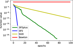
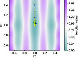
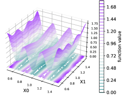
Figure 5: The Levy N. 13 function where Left: we plot $f(x)$ across epochs Middle: level set plot, Right: Surface plot. SP2 is in blue , SP2⁺ is in green , SGD is in yellow and Newton is in red .

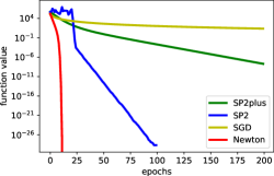
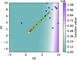
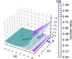
Figure 6: The Rosenbrock function where Left: we plot $f(x)$ across epochs Middle: level set plot, Right: Surface plot. SP2 is in blue , SP2⁺ is in green , SGD is in yellow and Newton is in red .

D.2 Additional Convex Experiments

We set the desired tolerance for each algorithm to $0.01$, and set the maximum number of epochs for each algorithm to $200$ in colon-cancer and 30 in mushrooms. To choose an optimal slack parameter $\lambda$ for SP2L2⁺, SP2L1⁺, and SP2max⁺, we test these three methods on a uniform grid $\lambda\in\{0.1,0.2,\ldots,0.9\}$ with $\sigma=0.001$. The gradient norm and loss evaluated at each epoch are presented in Figures 7-10 (see Appendix D). It can be seen that SP2L2⁺ performs best when $\lambda=0.9$ in colon-cancer and $\lambda=0.1$ in mushrooms, SP2L1⁺ and SP2max⁺ perform best when $\lambda=0.1$ in both data sets. Therefore, we set $\lambda=0.9$ for SP2L2⁺ in colon-cancer and fix $\lambda=0.1$ in other cases.

Under the same setting as in Section 6.3, we also compare the SP2max and SP2max⁺ methods on a grid $\lambda=[0.001~{}0.01:0.01:0.05]$ with $\sigma=0$. The gradient norm and loss evaluated at each epoch are presented in Figures 11-12 (see Appendix D). As we observe, SP2max⁺ always outperforms the SP2max method.

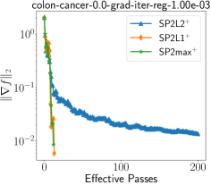
(a) $\lambda=0.1$

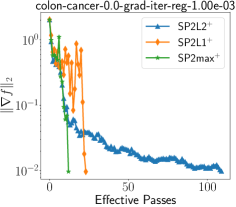
(b) $\lambda=0.2$

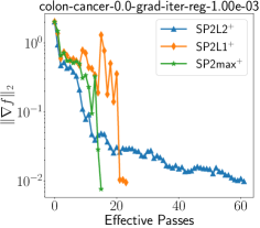
(c) $\lambda=0.3$

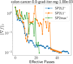
(d) $\lambda=0.4$

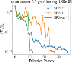
(e) $\lambda=0.5$

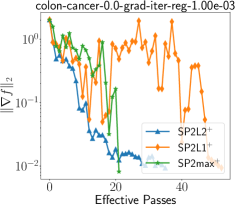
(f) $\lambda=0.6$

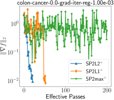
(g) $\lambda=0.7$

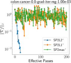
(h) $\lambda=0.8$

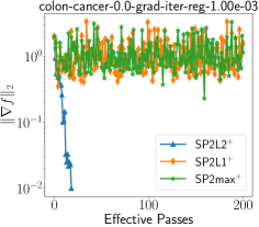
(i) $\lambda=0.9$

Figure 7: Colon-cancer: gradient norm at each epoch with different $\lambda$.

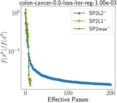
(a) $\lambda=0.1$

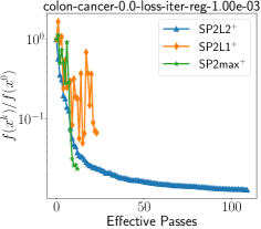
(b) $\lambda=0.2$

(c) $\lambda=0.3$

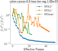
(d) $\lambda=0.4$

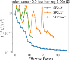
(e) $\lambda=0.5$

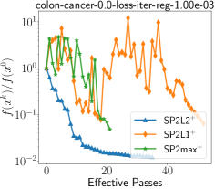
(f) $\lambda=0.6$

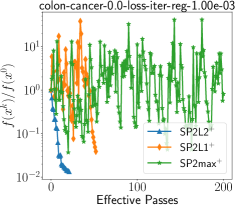
(g) $\lambda=0.7$

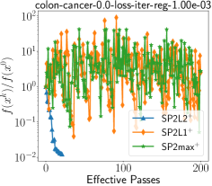
(h) $\lambda=0.8$

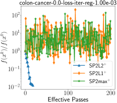
(i) $\lambda=0.9$

Figure 8: Colon-cancer: loss at each epoch with different $\lambda$.

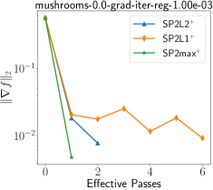
(a) $\lambda=0.1$

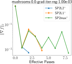
(b) $\lambda=0.2$

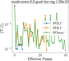
(c) $\lambda=0.3$

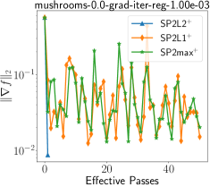
(d) $\lambda=0.4$

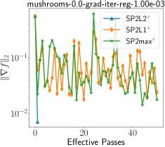
(e) $\lambda=0.5$

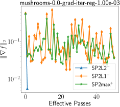
(f) $\lambda=0.6$

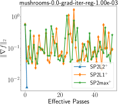
(g) $\lambda=0.7$

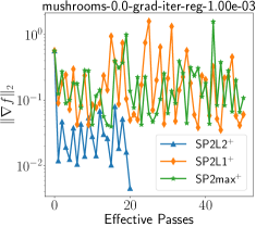
(h) $\lambda=0.8$

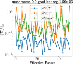
(i) $\lambda=0.9$

Figure 9: Mushrooms: gradient norm at each epoch with different $\lambda$.

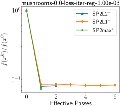
(a) $\lambda=0.1$

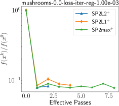
(b) $\lambda=0.2$

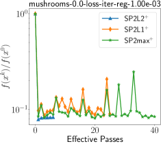
(c) $\lambda=0.3$

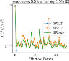
(d) $\lambda=0.4$

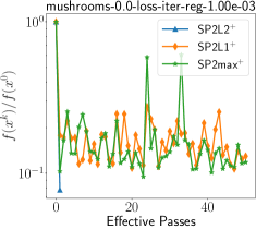
(e) $\lambda=0.5$

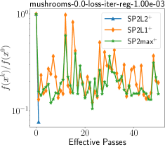
(f) $\lambda=0.6$

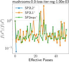
(g) $\lambda=0.7$

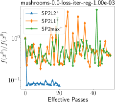
(h) $\lambda=0.8$

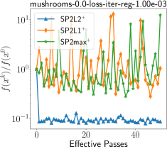
(i) $\lambda=0.9$

Figure 10: Mushrooms: loss at each epoch with different $\lambda$.

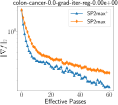
(a) $\lambda=0.001$

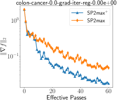
(b) $\lambda=0.01$

(c) $\lambda=0.02$

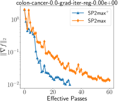
(d) $\lambda=0.03$

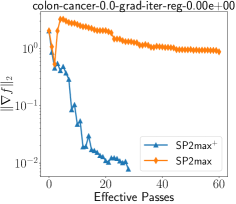
(e) $\lambda=0.04$

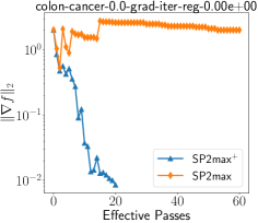
(f) $\lambda=0.05$

Figure 11: Colon-cancer: gradient norm at each epoch with different $\lambda$.

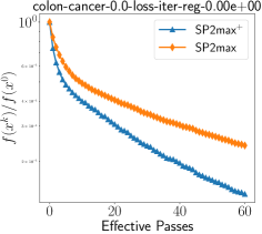
(a) $\lambda=0.001$

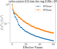
(b) $\lambda=0.01$

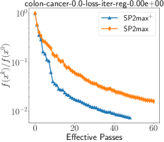
(c) $\lambda=0.02$

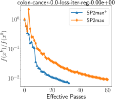
(d) $\lambda=0.03$

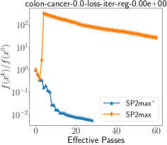
(e) $\lambda=0.04$

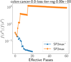
(f) $\lambda=0.05$

Figure 12: Colon-cancer: loss at each epoch with different $\lambda$.

References

• [1] N. Agarwal, B. Bullins, and E. Hazan. Second-order stochastic optimization for machine learning in linear time. Journal of Machine Learning Research, 18(116):1–40, 2017.
• [2] U. Alon, N. Barkai, D. A. Notterman, K. Gish, S. Ybarra, D. Mack, and A. J. Levine. Broad patterns of gene expression revealed by clustering analysis of tumor and normal colon tissues probed by oligonucleotide arrays. Proceedings of the National Academy of Sciences, 96(12):6745–6750, 1999.
• [3] A. S. Berahas, J. Nocedal, and M. Takáč. A multi-batch l-bfgs method for machine learning. In The Thirtieth Annual Conference on Neural Information Processing Systems (NIPS), 2016.
• [4] L. Berrada, A. Zisserman, and M. P. Kumar. Training neural networks for and by interpolation. In Proceedings of the 37th International Conference on Machine Learning, volume 119 of Proceedings of Machine Learning Research, pages 799–809, 13–18 Jul 2020.
• [5] R. Bollapragada, R. H. Byrd, and J. Nocedal. Exact and inexact subsampled Newton methods for optimization. IMA Journal of Numerical Analysis, 39(2):545–578, 04 2018.
• [6] R. H. Byrd, G. M. Chin, W. Neveitt, and J. Nocedal. On the use of stochastic Hessian information in optimization methods for machine learning. SIAM Journal on Optimization, 21(3):977–995, 2011.
• [7] J. Chen, R. Yuan, G. Garrigos, and R. M. Gower. San: Stochastic average newton algorithm for minimizing finite sums, 2021.
• [8] B. Christianson. Automatic Hessians by reverse accumulation. IMA Journal of Numerical Analysis, 12(2):135–150, 1992.
• [9] K. Crammer, O. Dekel, J. Keshet, S. Shalev-Shwartz, and Y. Singer. Online passive-aggressive algorithms. J. Mach. Learn. Res., 7:551–585, 2006.
• [10] Y.-H. Dai. Fast algorithms for projection on an ellipsoid. SIAM Journal on Optimization, 16(4):986–1006, 2006.
• [11] M. A. Erdogdu and A. Montanari. Convergence rates of sub-sampled Newton methods. In Advances in Neural Information Processing Systems 28, pages 3052–3060. Curran Associates, Inc., 2015.
• [12] R. M. Gower, M. Blondel, N. Gazagnadou, and F. Pedregosa. Cutting some slack for sgd with adaptive polyak stepsizes. arXiv:2202.12328, 2022.
• [13] R. M. Gower, A. Defazio, and M. Rabbat. Stochastic polyak stepsize with a moving target. arXiv:2106.11851, 2021.
• [14] R. M. Gower, D. Goldfarb, and P. Richtárik. Stochastic block BFGS: Squeezing more curvature out of data. Proceedings of the 33rd International Conference on Machine Learning, 2016.
• [15] R. M. Gower, O. Sebbouh, and N. Loizou. Sgd for structured nonconvex functions: Learning rates, minibatching and interpolation. arXiv:2006.10311, 2020.
• [16] O. Hinder, A. Sidford, and N. S. Sohoni. Near-optimal methods for minimizing star-convex functions and beyond. arXiv preprint arXiv:1906.11985, 2019.
• [17] M. Jahani, X. He, C. Ma, D. Mudigere, A. Mokhtari, A. Ribeiro, and M. Takac. Distributed restarting newtoncg method for large-scale empirical risk minimization. 2017.
• [18] M. Jamil and X.-S. Yang. A literature survey of benchmark functions for global optimization problems. CoRR, abs/1308.4008, 2013.
• [19] C. Jin, S. M. Kakade, and P. Netrapalli. Provable efficient online matrix completion via non-convex stochastic gradient descent. Advances in Neural Information Processing Systems, 29, 2016.
• [20] J. M. Kohler and A. Lucchi. Sub-sampled cubic regularization for non-convex optimization. In Proceedings of the 34th International Conference on Machine Learning, volume 70, pages 1895–1904, 2017.
• [21] D. Kovalev, K. Mishchenko, and P. Richtarik. Stochastic Newton and cubic Newton methods with simple local linear-quadratic rates. arxiv:1912.01597, 2019.
• [22] Y. Liu and F. Roosta. Convergence of newton-mr under inexact hessian information. SIAM J. Optim., 31(1):59–90, 2021.
• [23] N. Loizou, S. Vaswani, I. Laradji, and S. Lacoste-Julien. Stochastic polyak step-size for sgd: An adaptive learning rate for fast convergence. arXiv:2002.10542, 2020.
• [24] S. Ma, R. Bassily, and M. Belkin. The power of interpolation: Understanding the effectiveness of SGD in modern over-parametrized learning. In ICML, volume 80 of JMLR Workshop and Conference Proceedings, pages 3331–3340, 2018.
• [25] A. Mokhtari, M. Eisen, and A. Ribeiro. Iqn: An incremental quasi-newton method with local superlinear convergence rate. SIAM Journal on Optimization, 28(2):1670–1698, 2018.
• [26] A. Mokhtari and A. Ribeiro. Global convergence of online limited memory BFGS. The Journal of Machine Learning Research, 16:3151–3181, 2015.
• [27] P. Moritz, R. Nishihara, and M. I. Jordan. A linearly-convergent stochastic L-BFGS algorithm. In International Conference on Artificial Intelligence and Statistics, volume 51, pages 249–258, 2016.
• [28] J. Park and S. Boyd. General heuristics for nonconvex quadratically constrained quadratic programming. arXiv preprint arXiv:1703.07870, 2017.
• [29] M. Pilanci and M. J. Wainwright. Newton sketch: A near linear-time optimization algorithm with linear-quadratic convergence. SIAM Journal on Optimization, 27(1):205–245, 2017.
• [30] B. Polyak. Introduction to optimization. New York, Optimization Software, 1987.
• [31] Z. Qu, P. Richtárik, M. Takáč, and O. Fercoq. SDNA: Stochastic dual Newton ascent for empirical risk minimization. In Proceedings of the 33rd International Conference on Machine Learning, 2016.
• [32] A. Rodomanov and D. Kropotov. A superlinearly-convergent proximal newton-type method for the optimization of finite sums. In Proceedings of The 33rd International Conference on Machine Learning, volume 48 of Proceedings of Machine Learning Research, pages 2597–2605. PMLR, 20–22 Jun 2016.
• [33] F. Roosta-Khorasani and M. W. Mahoney. Sub-sampled newton methods. Math. Program., 174(1-2):293–326, 2019.
• [34] W. Sosa and F. MP Raupp. An algorithm for projecting a point onto a level set of a quadratic function. Optimization, pages 1–19, 2020.
• [35] N. Tripuraneni, M. Stern, C. Jin, J. Regier, and M. I. Jordan. Stochastic cubic regularization for fast nonconvex optimization. In S. Bengio, H. Wallach, H. Larochelle, K. Grauman, N. Cesa-Bianchi, and R. Garnett, editors, Advances in Neural Information Processing Systems, volume 31, 2018.
• [36] X. Wang, S. Ma, D. Goldfarb, and W. Liu. Stochastic quasi-newton methods for nonconvex stochastic optimization, 2017.
• [37] M. West, C. Blanchette, H. Dressman, E. Huang, S. Ishida, R. Spang, H. Zuzan, J. A. Olson, J. R. Marks, and J. R. Nevins. Predicting the clinical status of human breast cancer by using gene expression profiles. Proceedings of the National Academy of Sciences, 98(20):11462–11467, 2001.
• [38] S. Wright and J. Nocedal. Numerical optimization. Springer Science, 35(67-68):7, 1999.