S.M.A.S.H.E.D. :
Standard Model Axion Seesaw Higgs Inflation
Extended for Dirac Neutrinos

Abstract

Inspired by the S.M.A.S.H. framework we construct a model that addresses the strong CP problem, axion dark matter, inflation and Dirac neutrino masses as well as leptogenesis. The model possesses only two dynamical scales, namely the SM breaking scale $v_{H}$ and the Peccei Quinn (PQ) breaking scale $v_{\sigma}$. We introduce heavy vector-like quarks in the usual KSVZ fashion to implement the PQ mechanism for the strong CP problem. To generate neutrino masses via a dimension six operator scaling as $m_{\nu}\sim v_{H}^{3}/v_{\sigma}^{2}$ we add heavy triplet and doublet leptons, which are vector-like under the SM but chiral under PQ symmetry. The model is free from the cosmological domain wall problem and predicts an axion to photon coupling which is about an order of magnitude larger than in conventional DFSZ and KSVZ models. Thus our scenario can be probed and potentially excluded by current and next generation axion experiments such as ORGAN or MADMAX. In addition we numerically demonstrate that our construction can generate the observed baryon asymmetry by realizing a version of the Dirac-Leptogenesis scenario. As a consequence of our neutrino mass mechanism we find that the asymmetry in triplet fermion decays can also be significantly enhanced by up to six orders of magnitude when compared to typical Seesaw scenarios without needing to invoke a resonant enhancement. In passing we note that a decaying Dirac fermion with multiple decay modes contains all the necessary ingredients required for the quasi optimal efficiency-scenario previously encountered in the context decaying scalar triplets. The impact of the right handed neutrinos and the axion on $\Delta N_{\text{eff}}$ is estimated and lies within current bounds.

1 Introduction

Reductionism has been one of the most widely used approaches to building particle physics models that are supposed to address the theoretical, aesthetical and phenomenological gaps in the Standard Model (SM). For many decades the most common top-down approach consisted in unifying the SM gauge symmetries into single larger non-abelian Lie groups. This strategy led to the discovery of economical scenarios such as the Type I Seesaw-mechanism [1, 2, 3, 4, 5, 6] addressing both laboratory observations like neutrino masses and mixing as well as important cosmological issues such as the baryon asymmetry of the universe via leptogenesis [7]. In more recent years the focus has shifted to bottom-up approaches realizing the wanted phenomenology often via amending the SM with only a single additional global or gauged $\text{U}(1)$ factor. The most prominent examples of this latter category are the $\nu$MSM [8, 9, 10], which consists of a Type I Seesaw with the lightest right handed neutrino being a good dark matter (DM) candidate, as well as the S.M.A.S.H. proposal [11, 12, 13]. Here solutions to the strong CP problem, neutrino masses, electroweak vacuum stability, dark matter, inflation and baryogenesis via leptogenesis are possible by combining a Type I Seesaw with a global anomalous $\text{U}(1)_{\text{PQ}}$ Peccei-Quinn symmetry playing the role of spontaneously broken lepton number. Building on an earlier construction [14] inspired by the KSVZ [15, 16] axion model this framework identifies the mass scale of the heavy right handed neutrinos with the PQ breaking scale that in turn corresponds to the decay constant of the QCD axion (see also [17] for a similar setup where the right handed neutrino mass does not arise from PQ breaking). There also exists a class of related models based on the DFSZ [18, 19] approach see [20] for a recent example. Only two mass scales are present in the S.M.A.S.H. scenario: the electroweak breaking scale from the vacuum expectation value (vev) of the Higgs doublet scalar and the much larger vev of the PQ breaking singlet whose imaginary part is the axion. No new physics other than the PQ charged sector is needed up to the Planck scale. Most theories beyond the SM address the neutrino mass issue via mechanisms inducing parametrically light Majorana masses since this usually involves the smallest amount of new unknown coupling constants and Weyl spinors. However a priori in the absence of any experimental signal there is no reason to focus only on Majorana neutrinos, which is why there has been renewed interest in building Dirac neutrino mass model (see [21, 22, 23, 24, 25, 26, 27] for some explicit models and [28, 29, 30] for systematic studies just to name a few). In this work we set out to extend the S.M.A.S.H. class of models for light Dirac neutrinos. We outline the particle content and the most important interactions for the low energy phenomenology in section 2. Section 4 serves a brief summary of the cosmological history and most important parameters for the original S.M.A.S.H. scenario. The main focus of this work is Dirac-Leptogenesis in section 5. A novel way to enhance the leptonic asymmetry parameter from heavy fermion decays is presented in subsection 5.3. Analytical estimates in 5.4 help us narrow down the relevant parameter space and we show the validity of our scenario by numerically solving the Boltzmann equations from section 5.5 in subsection 5.6. In the aforementioned section we also demonstrate that the efficacy for asymmetry production from Dirac fermions can be larger than for Majorana fermions similar to [31] for decaying scalar triplets. After estimating the amount of dark radiation in section 6 we summarize our findings in 7. Additional relevant information was collected in appendices A-D.

2 The model

field	$\text{SU(3)}_{\text{C}}$	$\text{SU}(2)_{\text{L}}$	$\text{U}(1)_{\text{Y}}$	$\text{U}(1)_{\text{PQ}}$	generations
$q_{L}$	3	2	$1/6$	0	3
$u_{R}$	3	1	$2/3$	0	3
$d_{R}$	3	1	$-1/3$	0	3
$L$	1	2	$-1/2$	1	3
$e_{R}$	1	1	$-1$	1	3
$H$	1	2	$1/2$	0	1
$Q_{L}^{(1,2)}$	3	1	$2/3$ or $-1/3$	1	2
$Q_{R}^{(1,2)}$	3	1	$2/3$ or $-1/3$	0	2
$Q_{L}^{(3)}$	3	1	$2/3$ or $-1/3$	-1	1
$Q_{R}^{(3)}$	3	1	$2/3$ or $-1/3$	0	1
$T_{L}$	1	3	0	2	3
$T_{R}$	1	3	0	1	3
$D_{L}$	1	2	$1/2$	3	3
$D_{R}$	1	2	$1/2$	2	3
$\nu_{R}$	1	1	0	3	3
$\sigma$	1	1	0	1	1

Table 1: Charges and Representations under the SM gauge group and $\text{U}(1)_{\text{PQ}}$.

One way to generate tiny Dirac masses is the Type I Dirac-Seesaw scheme pioneered in [32]. In general one starts out by imposing a symmetry to forbid the tree-level Dirac neutrino mass term

$$\overline{L}\epsilon H^{\dagger}\nu_{R}$$ (2.1)

with $\epsilon=i\tau_{2}$ being the second Pauli matrix, as well as all possible Majorana masses. Then heavy vector-like SM singlet fermions coupling to both the SM leptons and $\nu_{R}$ are integrated out at energies below their mass scale leading to light neutrino masses from the threshold correction. Most models realize the neutrino mass via a dimension five operator similar to the Weinberg operator [33] of the schematic form $(LH)^{2}$ for Majorana neutrinos. Since the $\nu_{R}$ are SM singlets this necessitates the inclusion of a scalar singlet $\phi$ to form the required operator $(\overline{L}\epsilon H^{\dagger})\phi\nu_{R}$. The vev of $\phi$ introduces a third scale $v_{\phi}$ apart from the SM Higgs vev $v_{H}$ and the heavy mediator scale $M\gg v_{\phi},v_{H}$. Dirac masses then scale as $m_{\nu}\sim v_{H}v_{\phi}/M$ and the additional parameters are the reason why these scenarios are considered to be less minimal than Majorana models. If we wish to generate this operator via PQ charged particles and a singlet scalar $\sigma$ for spontaneous symmetry breaking of $\text{U}(1)_{\text{PQ}}$ there are essentially two options: One can either identify the heavy mass scale with the PQ breaking scale $M\sim v_{\sigma}$ as was the case for combining the Type I Seesaw with PQ symmetry in [14]. This then requires that $\phi$ is a third scalar field and $v_{H}\lesssim v_{\phi}\ll v_{\sigma}$. The other option is to identify $\phi$ with the PQ breaking field $\sigma$ [34] and assume a separate source for the heavy vector-like fermion masses. However since cosmological and astrophysical arguments require $v_{\sigma}>${10}^{8}\text{\,}\mathrm{GeV}$$ or even $v_{\sigma}\simeq${10}^{11}\text{\,}\mathrm{GeV}$$ (see subsection 4.2) the mediator mass scale must be potentially close to the Planck scale even for small Yukawa couplings [34]. Our model will be able to avoid these complications altogether. The key idea is that we can connect $L$ and $\nu_{R}$ by integrating out two different species of vector-like fermions transforming non-trivially under the electroweak gauge symmetry. To avoid a third scale besides $v_{H}$ and $v_{\sigma}$ we will generate the required threshold correction via a dimension six operator of the schematic form $(\overline{L}\epsilon H^{\dagger})(HH^{\dagger})\nu_{R}$. The heavy fermion masses scale with $v_{\sigma}$ and the presence of three Higgs doublets follows from the required $\text{SU}(2)_{\text{L}}$ contractions. In addition to that the active neutrino masses scale as $m_{\nu}\sim v_{H}^{3}/v_{\sigma}^{2}$. Before we face the neutrino sector we briefly review the KSVZ-axion model, which solves the strong CP problem via heavy vector-like fermions with PQ charge.

2.1 KSVZ-axion

In order to implement the Peccei-Quinn solution [35, 36] to the strong CP problem in the KSVZ model [15, 16] we introduce a pair of color triplet quarks $\left(Q_{L},Q_{R}\right)$, which are vector-like under the SM but chiral under PQ as well as a singlet scalar $\sigma$ coupling via

$$\mathcal{L}_{\text{KSVZ}}=-Y_{Q}\;\sigma\;\overline{Q_{L}}Q_{R}+\text{h.c.}\;\;.$$ (2.2)

The charges and representations under all symmetries can be found in table 1. The scalar potential reads

$$V(H,\sigma)=V(H)-\mu_{\sigma}^{2}\left|\sigma\right|^{2}+\lambda_{\sigma}\left|\sigma\right|^{4}+\lambda_{\sigma H}\left|\sigma\right|^{2}\left|H\right|^{2},$$ (2.3)

with $\mu_{\sigma}^{2}>0$ for the SSB of PQ symmetry and $V(H)$ the SM scalar potential. We expand the singlet scalar as

$$\sigma=\frac{1}{\sqrt{2}}\left(v_{\sigma}+\rho_{\sigma}\right)e^{i\frac{a}{v_{\sigma}}}\quad\text{with}\quad v_{\sigma}\gg v_{H}=$246\text{\,}\mathrm{GeV}$,$$ (2.4)

where $a$ denotes the axion field and we see that the exotic quarks have a mass term consisting of

$$M_{Q}\equiv Y_{Q}\frac{v_{\sigma}}{\sqrt{2}}.$$ (2.5)

After rotating the axion field away by an anomalous Peccei-Quinn transformation of the quarks [37] we can integrate them out and obtain the axion coupling to the QCD anomaly term. For $\text{SU}(2)_{\text{L}}$ singlets the QCD anomaly coefficient reads [38]

$$N=\sum_{\psi}\chi_{\psi}\;T_{d}(\psi),$$ (2.6)

where $T_{d}$ is the Dynkin color index for a $d$-dimensional representation with $T_{3}(Q_{L})=T_{3}(Q_{R})=1/2$ and $\chi_{\psi}$ denotes the PQ charge of the particle $\psi$. If we assume only one generation of exotic quarks then

$$N=\frac{1}{2}\left(\chi_{Q_{L}}-\chi_{Q_{R}}\right)=\frac{1}{2}\chi_{\sigma}.$$ (2.7)

The non-linearly realized $\text{U}(1)_{\text{PQ}}$ symmetry is explicitly broken by the non-perturbative QCD effects down to a $\mathcal{Z}_{2N}$ once the temperature of the universe cools below the QCD phase transition at $T=\Lambda_{QCD}=\mathcal{O}(200\;\text{MeV})$. The aforementioned QCD effects manifest themselves in an effective cosine potential and thus a mass for the axion $a$, which dynamically relaxes to its minimum to cancel the strong CP violation [35, 36] encoded in $\theta_{\text{QCD}}+\theta_{\text{weak}}$. In this context $\theta_{\text{QCD}}$ is the topological angle of QCD and $\theta_{\text{weak}}$ is the contribution from the chiral transformations needed to diagonalize the SM quark masses. After the angular mode $a$ relaxes in one of the $2N$ equivalent vacua, topological defects in the form of domain walls are formed from the spontaneous breaking of this discrete symmetry [39, 40, 41]. The cosmological domain wall number is given by $N_{\text{DW}}=2N$ and stable domain walls could overclose the universe [42, 43]. The domain walls form a network with axionic strings produced during the SSB of PQ symmetry via the Kibble mechanism [44, 45, 46], and the network will in general be stable for $N_{\text{DW}}>1$. For $N_{\text{DW}}=1$ the network eventually decays to low momentum axions [47, 48] and contributes to their relic density [49, 50, 51]. Pre-inflationary PQ breaking can dilute the domain walls and explicitly PQ breaking bias-terms in the scalar potential [43, 52, 53, 54] could make the domain walls decay. However we will see in section 4.2 that S.M.A.S.H. is only compatible with post-inflationary PQ breaking. Bias terms have to be large enough to make the domain walls decay before they dominate the energy density of the universe [55]. On the other hand, they have the drawback of contributing to the axion mass, so that one needs to ensure, that they do not spoil the PQ solution to the strong CP problem, leading to an upper limit on the corresponding coupling [55, 56]. There exists a parameter space that satisfies both conditions. The last class of solutions to the domain wall problem embeds the $\mathcal{Z}_{2N}$ into the center of a larger continuous global or local group [57, 58]. However we prefer to avoid these complications altogether by simply normalizing the PQ charges of the quarks properly. We demand $N_{\text{DW}}=1$, from which we deduce that $\chi_{\sigma}=1$. In this scenario we have an axion decay constant of

$$f_{a}\equiv\frac{v_{\sigma}}{N_{\text{DW}}}.$$ (2.8)

If one wishes to incorporate more generations of exotic quarks without generating additional domain walls then one has to make sure that the QCD anomaly coefficients for the additional generations cancel each other, for example by choosing equal and opposite PQ charges for those two generations. This explains the charge assignments for the third generation of exotic quarks in 1. At the present stage the exotic quarks would be absolutely stable owing to their separately conserved baryon number [15]. This would lead to exotic hadrons which could also overclose the universe and are tightly constrained relative to ordinary baryons by dedicated searches [59, 60]. In order to make the exotic quarks decay we introduce a renormalizable coupling to the SM doublet quarks $q_{L}$ and consider the following operators for $\chi_{Q_{R}}=0$ [59, 60]

$$\mathcal{L}_{\text{decay}}=-Y_{qQ}\begin{cases}\overline{q_{L}}\epsilon H^{\dagger}Q_{R}\quad\text{for}\quad Y_{Q_{R}}=\frac{2}{3}\\ \overline{q_{L}}HQ_{R}\quad\text{for}\quad Y_{Q_{R}}=-\frac{1}{3}\end{cases}+\text{h.c.},$$ (2.9)

where $Y_{qQ}$ is a dimensionless Yukawa coupling to the SM Higgs. There will be a lower limit on the Yukawa coupling in (2.9) from demanding that decay rate (assuming $m_{Q}\gg m_{H}$)

$$\Gamma\left(Q\rightarrow q_{L}H\right)\simeq\frac{Y_{qQ}^{2}m_{Q}}{16\pi}$$ (2.10)

is faster than the Hubble rate at the temperature $T=m_{Q}$ implying

$$Y_{qQ}\gtrsim 10^{-5}\;\sqrt{\frac{m_{Q}}{10^{8}\;\text{GeV}}},$$ (2.11)

so that the abundance of vector-like quarks is actually depleted and an epoch of intermediate era of matter domination [61] from very long-lived vector-like quarks is avoided. In the above we used a value for $m_{Q}$ that will be motivated in section 4.3. Vector-like quarks could be produced at colliders, either in pairs from a gluon or together with an SM quark via the coupling in (2.9). Searches for new colored fermions exclude vector-like quark masses below about $1\;\text{TeV}$ [62, 63]. The large couplings together with heavy large masses are the reason, why we expect the life-time of the vector-like quarks, if kinematically accessible at colliders, to be very short.

2.2 Neutrino masses

Figure 1: Diagrammatic representation of the dimension 6 operator giving rise to Dirac masses for the active neutrinos.

In a similar spirit we now introduce vector-like leptons as well to generate the Dirac neutrino masses in the Seesaw fashion. We give vector-like PQ charges to the SM leptons and charge $\nu_{R}$ in such a way that the tree level mass term $\overline{L}\epsilon H^{\dagger}\nu_{R}$ with $\epsilon=i\tau_{2}$ being the second Pauli matrix is absent. Since the cosmologically preferred PQ breaking scale $f_{a}\simeq 10^{11}\;\text{GeV}$ is lower than the typical Seesaw-scale (for order one Yukawas) of $M_{N}\simeq 10^{14}\;\text{GeV}$ we choose to integrate out two distinct fermions instead of a single messenger. However these two fermion species will have comparable masses so this sequential Seesaw depicted in figure 1 does not lead to a double Seesaw-mechanism [64, 65]. The resulting operator for neutrino masses will have mass dimension six (see [29] for a compendium of possible Dirac dimension six operators) compared to the usual Weinberg operator at dimension five [33]. We start with introducing three generations of vector-like pairs of triplets $(T_{L},T_{R})$ and doublets $(D_{L},D_{R})$. The multiplets can be expanded into their components as

$$T_{L}\equiv\frac{T_{L}^{a}\tau^{a}}{2}=\begin{pmatrix}\frac{T_{L}^{0}}{\sqrt{2}}&T_{L}^{+}\\ T_{L}^{-}&-\frac{T_{L}^{0}}{\sqrt{2}}\end{pmatrix},\quad T_{R}\equiv\frac{T_{R}^{a}\tau^{a}}{2}=\begin{pmatrix}\frac{T_{R}^{0}}{\sqrt{2}}&T_{R}^{+}\\ T_{R}^{-}&-\frac{T_{R}^{0}}{\sqrt{2}}\end{pmatrix}$$ (2.12)

and

$$\quad D_{L}\equiv\begin{pmatrix}E_{L}^{+}\\ N_{L}\end{pmatrix},\quad D_{R}\equiv\begin{pmatrix}E_{R}^{+}\\ -N_{R}\end{pmatrix}.$$ (2.13)

We also introduce the following notation of $\tilde{H}\equiv\epsilon H^{\dagger}$. A combination of chiral PQ charges, Hypercharge and non-trivial $\text{SU(2)}_{\text{L}}$ representations allows only the following mass

$$\mathcal{L}_{\text{mass}}=-Y_{T}\sigma\overline{T_{L}}^{a}T_{R}^{a}-Y_{D}\sigma\overline{D_{L}}D_{R}+\text{h.c.}$$ (2.14)

and mixing terms

$$\mathcal{L}_{\text{int}}=-Y_{LT}\;\overline{L}\;T_{R}^{a}\tau^{a}\tilde{H}-Y_{TD}\;D_{R}\epsilon\;\overline{T_{L}}^{a}\tau^{a}\tilde{H}-Y_{DR}\;\overline{D_{L}}H\nu_{R}+\text{h.c.}\;.$$ (2.15)

All charges and representations for the four component spinors have been summarized in table 1. If we had given $D_{L,R}$ the opposite hypercharge $-1/2$ an operator of the schematic form $\overline{L}D_{R}\sigma^{*}$ would be allowed by all imposed symmetries and this operator would ruin the sequential nature of our mass generation mechanism by coupling $\nu_{L}$ directly to the exotic $N_{R}$ neutrino with a large vev $v_{\sigma}$. We use triplets $T_{L,R}$ instead of singlet fermions $S_{L,R}$ because the PQ charge assignment would allow for a term $\overline{S_{L}}\nu_{R}\sigma^{*}$, which would also spoil the intended mass generation mechanism. Note that if one identifies our unconventional chiral choice of PQ charges with lepton number or B-L, which are usually taken to have vector-like charges normalized to $\pm 1$, one can understood the “Diracness” of the neutrinos as follows: Since $\sigma$ breaks PQ symmetry by only a single unit all the renormalizable Majorana mass terms which would require breaking by two, four or six units (see table 1) are forbidden. This is in a similar spirit to the argument that breaking conventionally assigned lepton number or B-L by any number other than two allows only for Dirac neutrinos [21]. Of course PQ symmetry does not forbid the following non-renormalizable operators

$$\frac{c_{T_{R}}}{\Lambda_{\text{UV}}}\left(\sigma^{*}\right)^{2}\overline{T_{R}^{c}}^{a}T_{R}^{a},\quad\frac{c_{T_{L}}}{\Lambda_{\text{UV}}^{3}}\left(\sigma^{*}\right)^{4}\overline{T_{L}^{c}}^{a}T_{L}^{a},\quad\frac{c_{\nu_{R}}}{\Lambda_{\text{UV}}^{5}}\left(\sigma^{*}\right)^{6}\overline{\nu_{R}^{c}}\nu_{R},$$ (2.16)

as well as

$$\frac{c_{L}}{\Lambda_{\text{UV}}^{3}}\left(\sigma^{*}\right)^{2}\left(\overline{L^{c}}\epsilon H\right)\left(L\epsilon H\right),\quad\frac{c_{D_{R}}}{\Lambda_{\text{UV}}^{5}}\left(\sigma^{*}\right)^{4}\left(\overline{D_{R}^{c}}H^{\dagger}\right)\left(D_{R}H^{\dagger}\right),\quad\frac{c_{D_{L}}}{\Lambda_{\text{UV}}^{7}}\left(\sigma^{*}\right)^{6}\left(\overline{D_{L}^{c}}H^{\dagger}\right)\left(D_{L}H^{\dagger}\right),\quad$$ (2.17)

where the $c_{i}$ are dimensionless Wilson-coefficients and $\Lambda_{\text{UV}}$ is some mass scale above the PQ scale. Evidently the dimension five operator for $T_{R}$ is the least suppressed and the mass term for the $D_{L}$ at dimension eleven has the largest suppression factor due to SM gauge invariance and PQ breaking by six units. We have checked that these operators are not generated at loop level for the given particle content in field theory, but if one includes quantum gravity they might arise. Non-perturbative quantum gravitational effects could lead to a low energy effective field theory which will contain all the terms allowed by only the local gauge symmetries [38] such as the above ones. On top of that quantum gravity is expected to violate global symmetries [66, 67, 68] like PQ symmetry. These quantum gravity effects are heuristically encoded in Planck-mass suppressed explicitly PQ violating operators leading to the well known “axion quality problem” [71, 72, 73, 74, 75, 76] that could spoil the solution to the strong CP problem. PQ violating Majorana masses could arise in the same way too [77]. Since we have nothing to add to the solution of these “quality problems” we will assume that the Wilson coefficients of both sets of hypothetical effective operators (PQ conserving or violating) are either negligibly small or that some other mechanism prevents their existence.

Before EWSB the triplets and doublets are decoupled and each component of an $\text{SU(2)}_{\text{L}}$ multiplet has a common mass set by the PQ breaking scale, which we call

$$M_{T}\equiv Y_{T}\frac{v_{\sigma}}{\sqrt{2}}\quad\text{and}\quad M_{D}\equiv Y_{D}\frac{v_{\sigma}}{\sqrt{2}}.$$ (2.18)

After integrating them out and applying a Fierz-transformation we find

$$\mathcal{L}_{\text{eff.}}=\frac{1}{2}\;Y_{LT}M_{T}^{-1}Y_{TD}M_{D}^{-1}Y_{DR}\;\;\left(\overline{L}\epsilon H^{\dagger}\right)\left(HH^{\dagger}\right)\nu_{R}+\text{h.c.}\;.$$ (2.19)

In the one flavor approximation we find the following relation for the active neutrino mass scale after electroweak symmetry breaking (EWSB)

$$m_{\nu}\simeq$0.05\text{\,}\mathrm{eV}$\cdot Y_{LT}Y_{TD}Y_{DR}\cdot\left(\frac{${10}^{9}\text{\,}\mathrm{GeV}$}{M_{T}}\right)\cdot\left(\frac{${10}^{8}\text{\,}\mathrm{GeV}$}{M_{D}}\right).$$ (2.20)

If we choose $M_{T},M_{D}$ lighter than about $\mathcal{O}\left(${10}^{8}\text{\,}\mathrm{GeV}$\right)$ we can maintain the light neutrino mass scale by decreasing the Yukawa coupling $Y_{LT}Y_{TD}Y_{DR}$. On the other hand the overall neutrino mass scale could be lowered too far if we chose $M_{T},M_{D}\gg\mathcal{O}\left(${10}^{8}\text{\,}\mathrm{GeV}$\right)$, which is why we work in the previously mentioned regime. Since we expect $f_{a}\simeq\mathcal{O}\left(${10}^{11}\text{\,}\mathrm{GeV}$\right)$ (see (4.2)) this means that Yuakwa couplings of the $T,D$ fields to the PQ breaking field must satisfy $Y_{T,D}\lesssim 10^{-3}$. Here there are only two dynamical scales $v_{H}$ and $v_{\sigma}$ involved in the neutrino mass generation, which comes at the price of introducing five Yukawa matrices $Y_{LT},Y_{TD},Y_{DR},Y_{T},Y_{D}$. In order to generate the two mass splitting needed to explain the neutrino oscillation data we need to introduce at least two generations of $T_{L,R},D_{L,R}$ and in the following we will assume the existence of three such generations. We can estimate the axion decay constant

$$f_{a}\simeq$4\text{\times}{10}^{8}\text{\,}\mathrm{GeV}$\cdot\sqrt{\frac{$0.1\text{\,}\mathrm{eV}$}{m_{\nu}}}\cdot\sqrt{\frac{Y_{LT}Y_{TD}Y_{DR}}{Y_{T}Y_{D}}}$$ (2.21)

as a function of the active neutrino mass. If we drop the previous assumption about the Yukawa couplings and allow all five of them to vary between $\mathcal{O}(1)$ and $\mathcal{O}\left(10^{-6}\right)$ (which are the largest and smallest Yukawa couplings in the SM of the top quark and electron respectively), we find

$$$0.4\text{\,}\mathrm{GeV}$\cdot\sqrt{\frac{$0.1\text{\,}\mathrm{eV}$}{m_{\nu}}}\;\lesssim\;f_{a}\;\lesssim\;$4\text{\times}{10}^{14}\text{\,}\mathrm{GeV}$\cdot\sqrt{\frac{$0.1\text{\,}\mathrm{eV}$}{m_{\nu}}}.$$ (2.22)

The lower range of $f_{a}\sim$0.4\text{\,}\mathrm{GeV}$$ obtained for the extreme choice $Y_{LT}\sim Y_{TD}\sim Y_{DR}\sim 10^{-6}$ and $Y_{T}\sim Y_{D}\sim 1$ would correspond to the Weinberg-Wilczek [79, 80] axion which has been ruled out experimentally via meson decays a long time ago [81]. Furthermore astrophysical arguments based on stellar cooling demand $f_{a}>${10}^{8}\text{\,}\mathrm{GeV}$$, so that the region of small $Y_{LT}\sim Y_{TD}\sim Y_{DR}$ is already excluded. Note that having such small couplings would defeat the purpose of building a rather involved Seesaw model to begin with. We depict the decay constants that would lead to a too small neutrino mass as the grey region in the figures 3 and 3, which shall be the focus of the next subsection.

2.3 Axion to photon coupling

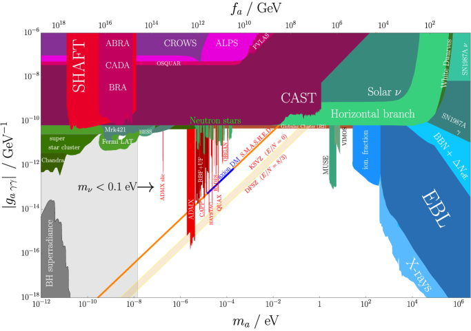
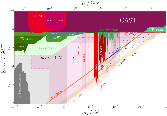
Figure 2: Depicted are the “S.M.A.S.H.E.D.” band in orange and the QCD-axion band for the KSVZ and DFSZ models in yellow as well as a collection of cosmological, astrophysical and laboratory constraints. The white space is allowed and in the gray area the active neutrino masses would be too small. The black arrow to the right indicates that the lower allowed limit on $m_{a}$ increases for larger values of $m_{\nu}$. The corresponding references can be found in appendix A.

Figure 3: Depicted are the “S.M.A.S.H.E.D.” band in orange and the QCD-axion band for the KSVZ and DFSZ models in yellow as well as cosmological, astrophysical and laboratory constraints together with projected sensitivities. The black arrow to the right indicates that the lower allowed limit on $m_{a}$ increases for larger values of $m_{\nu}$. The corresponding references can be found in appendix A.

The most relevant coupling for the direct detection of axions in laboratory experiments is the axion-to photon coupling, which is given by [82, 83]

$$g_{a\gamma\gamma}=\frac{\alpha}{2\pi f_{a}}\left(\frac{E}{N}-1.92(4)\right),$$ (2.23)

where the second term represents the model-independent irreducible contribution from the axion-pion mass mixing. The color anomaly coefficient $N$ was specified in equation (2.6) and is found to be $N=1/2$ for this model. The electromagnetic anomaly coefficient $E$ is defined via [38]

$$E=\sum_{\psi}\;\chi_{\psi}\;d_{c}(\psi)\;\text{Tr}\left(Q^{2}_{\text{EM}\;\psi}\right),$$ (2.24)

where $\chi_{\psi}$ is the PQ charge of the fermion $\psi$, $d_{c}(\psi)$ is the dimension of its color representation and $Q_{\text{EM}\;\psi}$ its electric charge matrix. For the original KSVZ model, where the exotic quarks have no hypercharge one finds $E/N=0$. Since we equip them with hypercharge for cosmological reasons (see table 1 for their charges) their contribution reads

$$\left(\frac{E}{N}\right)_{Q}=2\cdot 3\cdot\begin{cases}\frac{4}{9}\\ \frac{1}{9}\end{cases}=\begin{cases}\frac{8}{3}\quad\text{for}\quad Y_{Q_{L}}=\frac{2}{3},\\ \frac{2}{3}\quad\text{for}\quad Y_{Q_{L}}=-\frac{1}{3},\end{cases}$$ (2.25)

where the factor of three comes from $d_{c}(Q_{L})=3$. Only the first generation of exotic quarks contribute since we assume the PQ charges of the second and third generations cancel each other in order to fix the domain wall number. Similarly even though the SM leptons $L$ and $e_{R}$ have electric charge, they are vector-like under PQ and do not contribute to $E$. As a consequence of introducing non-trivial $\text{SU(2)}_{\text{L}}$ representations which are chiral under PQ for neutrino mass generation we obtain an additional contribution from the $T$ and $D$:

$$\left(\frac{E}{N}\right)_{T,D}=2\cdot 3\cdot(2+1)=18$$ (2.26)

The factor of three takes the three generations of exotic leptons into account and since each triplet contains two charged fermions their contribution is twice as large as for the doublets. Consequently the model dependent part of the axion to photon coupling

$$\left(\frac{E}{N}\right)_{\text{tot}}=18+\begin{cases}\frac{8}{3}\quad\text{for}\quad Y_{Q_{L}}=\frac{2}{3},\\ \frac{2}{3}\quad\text{for}\quad Y_{Q_{L}}=-\frac{1}{3}\end{cases}$$ (2.27)

is significantly larger than in conventional models such as the DFSZ I (II) scenario, where the ratio reads $8/3\;(2/3)$. Thus our neutrino mass mechanism has the additional benefit of making the axion easier to detect in laboratory experiments. Compared to other constructions in the literature this enhancement is rather small. For comparison clockwork based models such as [84, 85, 86] lead to an exponential enhancement of the coupling, a recent construction with quantized magnetic charges [87, 88] can increase the axion to photon coupling by six orders of magnitude. Mirror sector models with $n$ copies of the SM and PQ sectors [89, 90] can increase the axion to photon coupling as a function of $n$ by lowering the axion mass compared to the usual QCD axion. Alternatively if one sticks to the particle content of the KSVZ model then the largest possible positive anomaly coefficient was found to be $E/N=170/3$ [59, 60]. A recent scan over possible representations found that $E/N=-166/3$ [91] is the largest possible negative value within the range of the scan. Note that the two previously mentioned scenarios require three or eight quarks of different SM representations. We depict the experimentally allowed parameter space and a collection of limits in 3 together with the projections form upcoming searches in 3. The limits and projected limits were compiled in [92] and they can be found in appendix A. The orange band dubbed “S.M.A.S.H.E.D.” corresponds to the prediction of our model. Inside this band there is a blue region called “axion DM” which reproduces the observed DM abundance for the cosmological history of the S.M.A.S.H. models and will be explained in section 4.2. Experiments like QUAX [93, 94] or HAYSTAC [95, 96] have already started to test the relevant parameter space depicted in blue. Other experiments like ORGAN [97, 98] or RADES [99] are close to probing the axion DM parameter space as can be seen in 3. When it comes to next generation experiments we find that MADMAX [100], the upgraded ADMX experiment [101, 102, 103, 104, 105, 106, 107, 108] as well as BRASS [109] have good chances of testing the aforementioned parameter region. In appendix B we demonstrate numerically that the new heavy fermions do not lead to phenomenologically relevant Landau poles in any of the SM gauge couplings following the treatments in [110, 111, 91].

2.4 Axion to fermion coupling

The chiral rotations that remove the phase of the singlet field $\sigma$ from the mass terms induce the following derivative interactions for all PQ charged fermions $\Psi$ with chiral charges $\chi_{L,R}$

$$\mathcal{L}_{\text{int.}}=i\frac{\partial_{\mu}a}{f_{a}}\sum_{\Psi}\overline{\Psi}\gamma^{\mu}\left(\frac{\chi_{L}+\chi_{R}}{2}\cdot\mathbbm{1}_{4}-\frac{\chi_{L}-\chi_{R}}{2}\cdot\gamma_{5}\right)\Psi.$$ (2.28)

The only SM fermions that pick up an interaction at tree level are the three generations of charged and neutral leptons:

$$\mathcal{L}_{\text{int.}}=i\frac{\partial_{\mu}a}{f_{a}}\sum_{j}\left(\overline{e}_{j}\gamma^{\mu}e_{j}+\overline{\nu}_{j}\gamma^{\mu}\left(2\cdot\mathbbm{1}_{4}+\gamma_{5}\right)\nu_{j}\right)$$ (2.29)

As expected the charged lepton coupling is vector-like. If we integrate the first term by parts we pick up a contribution of

$$\sum_{j}\partial_{\mu}\left(\overline{e}_{j}\gamma^{\mu}e_{j}\right)$$ (2.30)

which vanishes for on shell leptons. Of course as in the original KSVZ model a pseudoscalar coupling to will be regenerated at loop level from the axion to photon coupling in (2.23) [14]

$$g_{ae}\simeq\alpha\;g_{a\gamma\gamma}\;m_{e}\;\text{Log}\left(\frac{f_{a}}{m_{e}}\right),$$ (2.31)

which is dimensionless as $g_{a\gamma\gamma}\sim 1/f_{a}$. Here we neglected the contribution from axion pion mixing in (2.23) as it was subdominant to the inclusion of the heavy exotic fermions. One can see that this coupling $g_{ae}\simeq 3\times 10^{-17}$ is very small due to its dependence on $\alpha\;m_{e}/f_{a}$. There are more one loop contributions to $g_{ae}$ from one loop diagrams involving the other massive EW gauge bosons as well as the new exotic fermions. By recasting the result for a Majorana Type I Seesaw from [14, 112] we estimate

$$g_{ae}\simeq\frac{1}{16\pi^{2}}\left(\frac{m_{\nu}}{v_{H}}\right)^{2}\frac{m_{e}}{f_{a}}.$$ (2.32)

This contributions is suppressed by both $m_{e}/f_{a}\simeq 5\times 10^{-15}$ and $m_{\nu}^{2}/v_{H}^{2}\simeq 10^{-25}$ so we do not consider them further. Stellar cooling arguments for the sun and red giants exclude $g_{ae}\gtrsim\mathcal{O}\left(10^{-13}\right)$ [113, 114, 115, 116], which is respected by our model. Axions could also be emitted in laboratory experiments from the final state neutrino or charged lepton in pseudoscalar-meson decay. Since this will remove the chirality suppression of the two-body decay, these channels are sensitive probes for new physics. Existing analyses [117, 118, 119, 120] (often) do not use the full derivative coupling in (2.29) but rely on Yukawa-interactions which are technically only valid for on-shell fermions [121, 122]. However since the full calculation can involve technical subtleties such as infrared-divergences which have to be cancelled via loop-corrections [119] we will limit ourselves to recasting the existing limits. For the emission from a neutrino line we replace the axion neutrino coupling with $g_{\nu}=m_{\nu}/f_{a}$. Reference [119] found that depending on the flavor-structure $g_{\nu}^{2}<\mathcal{O}\left(10^{-6-7}\right)$ which translates to

$$f_{a}>\mathcal{O}(10^{3})\;\times m_{\nu}$$ (2.33)

and is not restrictive at all.

3 Unification

The DFSZ [18, 123] version of the original S.M.A.S.H. framework avoids the exotic vector-like quarks by charging the SM quarks under PQ symmetry and was discussed in [13]. Since this variant of S.M.A.S.H. only requires an additional gauge singlet sterile neutrino $N$, one can embed the DFSZ-S.M.A.S.H. in a basic Grand Unified Theory (GUT): One can choose $\text{SU}(5)$ [124, 125] by introducing $N$ as an additional singlet or pick the larger $\text{SO}(10)$ [126, 125], where $N$ fills the 16-dimensional spinorial representation together with the other 7 Weyl spinors for one generation of the SM. For a Type I Dirac Seesaw one can also find an $\text{SO}(10)$-embedding by introducing the SM gauge singlet vector-like neutrinos as $\text{SO}(10)$-singlets [34]. In our case of S.M.A.S.H.E.D. the situation is not as straight-forward, because we introduce vector-like fermions transforming non-trivially under the SM gauge group. This is why we would need to fill additional multiplets of e.g. $\text{SO}(10)$, which comes at the price of introducing additional fermions for anomaly cancellation. One can see, that there is no obvious GUT-embedding of our setup and further work would be required to find one.

4 Cosmology of S.M.A.S.H.

We briefly recapitulate the most important aspects of the cosmological history in the S.M.A.S.H. framework [11, 12, 13].

4.1 Inflation and reheating

Scalar fields with a non-minimal coupling to scalar curvature [127, 128, 129, 130, 131, 132, 133, 134] are chosen as the inflationary scenario. In a two field model, such as the present setup featuring the neutral component of $H$ together with $\sigma$, the inflationary dynamics are more complicated, which is why the authors of [11, 12, 13] worked out limiting cases, in which effectively only one field is responsible for inflation. Because of the unitarity problem [135, 136, 137] for pure Higgs inflation (HI) [138, 139, 140] reference [12] considered the inflaton to be either arising from the field $\sigma$ (HSI scenario) or as a linear combination of the neutral component of $H$ and $\sigma$ (HHSI scenario). One finds the valleys of the potential, that are attractors for the inflationary trajectories, by inspecting the signs of the following quantities [12]

$$\kappa_{H}\equiv\lambda_{H\sigma}\xi_{H}-\lambda_{H}\xi_{\sigma},\quad\kappa_{\sigma}\equiv\lambda_{H\sigma}\xi_{\sigma}-\lambda_{\sigma}\xi_{H}.$$ (4.1)

The relevant ranges are $\kappa_{H}>0\;\wedge\kappa_{\sigma}>0$ (here $\wedge$ is a logical “and”) for either HI or HSI, whereas HHSI needs $\kappa_{H}<0\;\wedge\kappa_{\sigma}<0$. Solving the unitarity problem requires $0<\xi_{\sigma}\lesssim 1$ [12] for the coupling to gravity. In this context and because of vacuum stability (see 4.3) for HHSI one needs a trajectory that is parametrically close to the HSI one, which can be achieved in the limit $\xi_{H}\ll\xi_{\sigma}$ [12]. Then one finds that the radial modes of the SM like Higgs and $\sigma$ lead to the following inflationary trajectory [12]

$$\frac{\rho_{\sigma}}{\rho_{H}}=\sqrt{-\frac{\lambda_{H}}{\lambda_{H\sigma}}}+\mathcal{O}\left(\frac{\xi_{H}}{\xi_{\sigma}}\right),$$ (4.2)

where $\lambda_{H\sigma}<0$ is required for HHSI [12]. On the other hand $\lambda_{H\sigma}>0$ selects HI and HSI. In the HSI scenario non-thermal axions get produced during reheating after the non-thermal restoration of PQ symmetry (see the next subsection 4.2). This scenario has a reheating temperature of around $10^{7}\;\text{GeV}$ that is so low that the axions never thermalize (see section 6.1), leading to an abundance of dark radiation $\Delta N_{\text{eff.}}\simeq 0.35-1.6$ [12] which is excluded by observations [141]. Therefore only the HHSI scenario is viable. In this regime the effective quartic coupling for inflation reads

$$\tilde{\lambda}_{\sigma}\equiv\lambda_{\sigma}-\frac{\lambda_{H\sigma}^{2}}{\lambda_{H}}$$ (4.3)

and it is bounded by [12]

$$5\times 10^{-10}<\tilde{\lambda}_{\sigma}<5\times 10^{-13},$$ (4.4)

where the upper limit comes from the amplitude of primordial scalar perturbations and the lower limit from the bound on the tensor to scalar ratio [142, 141]. Reheating occurs via damped inflaton oscillations in a quartic potential. The dominant channel is the production of EW gauge bosons from the inflaton’s SM like Higgs component during zero crossings of the oscillating condensate. The EW gauge bosons have effective inflaton dependent masses and decay efficiently to SM fermions as the gauge boson masses increase away from the crossings. During the zero crossings gauge boson production from the resulting fermion bath is also efficient. Due to their mass gain and the fact that the gauge bosons decay to fermions before they can loose this energy to the condensate again, energy is efficiently drained from the inflaton to the SM fermion bath. Production of the heavy exotic fermions occurs as well, but since their decays to SM fermions are suppressed compared to the gauge bosons, their inclusion is negligible. The reheating temperature can be estimated to be [12]

$$T_{\text{RH}}\simeq 10^{9}\;\text{GeV}\;\cdot\left(\frac{\tilde{\lambda}_{\sigma}}{10^{-10}}\right)^{\frac{5}{8}}\cdot\left(\frac{g^{2}\left|\lambda_{H\sigma}\right|/(4\lambda_{H})}{0.03}\right)^{\frac{5}{8}},$$ (4.5)

where $g$ is a shorthand for the EW gauge couplings and we used typical parameters from the analysis of [12]. A recent reevaluation [143] of the preheating dynamics revealed that one can no longer neglect the exponential growth of fluctuations of the SM like Higgs after non-thermal restoration of PQ symmetry, because there are large fluctuations in the singlet direction, whose imaginary part lowers the effective Higgs mass. The new results [143] indicate that the reheating temperature can be as large as

$$T_{\text{RH}}=\left(10^{12}-10^{13}\right)\;\text{GeV}.$$ (4.6)

As it turns out the critical temperature for the PQ phase transition is $T_{c}\simeq 0.01\;f_{a}$ [12], which for $f_{a}<10^{11}\;\text{GeV}$ lies below the reheating temperature in (4.6) meaning that PQ symmetry is thermally restored in the HHSI case.

4.2 Axion dark matter

It is well known that the cosmological evolution of the axion depends on the fate of PQ symmetry during inflation [144]. In S.M.A.S.H. one finds that PQ symmetry is non-thermally restored during preheating [12] via the growth of $\sigma$-excitations that destroy the coherence of the inflaton condensate as long as

$$f_{a}\lesssim$4\text{\times}{10}^{16}\text{\,}\mathrm{GeV}$.$$ (4.7)

In case PQ symmetry was not restored only the misalignment mechanism [145, 146, 147] contributes to the axion DM abundance but this scenario leads to axion isocurvature fluctuations, which are tightly constrained [148]. Requiring the absence of these fluctuations imposes the condition [149]

$$f_{a}<$1.4\text{\times}{10}^{14}\text{\,}\mathrm{GeV}$,$$ (4.8)

implying that the non-restored scenario is ruled out. In the PQ restored scenario there are contributions from both axion misalignment and the decay of the network of topological defects (made up of domain walls and axionic strings see subsection 2.1) [47, 48, 39, 150, 151, 152, 153] which is unstable for $N_{\text{DW}}=1$. The contributions from the misalignment mechanism and the decay of the topological defects fits the observed DM relic density in the regime [12]

$$$3\text{\times}{10}^{10}\text{\,}\mathrm{GeV}$\lesssim f_{a}\lesssim$1.2\text{\times}{10}^{11}\text{\,}\mathrm{GeV}$,$$ (4.9)

which corresponds to axion masses of [12]

$$$50\text{\,}\mathrm{\SIUnitSymbolMicro eV}$\lesssim m_{a}\lesssim$200\text{\,}\mathrm{\SIUnitSymbolMicro eV}$.$$ (4.10)

A more recent study [154] found a compatible range of masses in the window $$40\text{\,}\mathrm{\SIUnitSymbolMicro eV}$\leq m_{a}\leq$180\text{\,}\mathrm{\SIUnitSymbolMicro eV}$$. In the case that the entire axion relic abundance comes from misalignment only, the precise value of the required axion mass for post-inflationary PQ breaking varies from study to study and some examples are $m_{a}=$14.6\pm 0.1\text{\,}\mathrm{\SIUnitSymbolMicro eV}$$ [155], $m_{a}=$18\text{\,}\mathrm{\SIUnitSymbolMicro eV}$$ [156] and $m_{a}=$25.2\pm 11.0\text{\,}\mathrm{\SIUnitSymbolMicro eV}$$ [157]. We show the corresponding parameter space $$14\text{\,}\mathrm{\SIUnitSymbolMicro eV}$\leq m_{a}\leq$200\text{\,}\mathrm{\SIUnitSymbolMicro eV}$$ for the axion to photon coupling as the blue interval labelled “axion DM” in the orange “S.M.A.S.H.E.D.”-band in figures 3 and 3. If one abandons the cosmological history of S.M.A.S.H. and assumes a sequestered sector for inflation, then pre-inflationary PQ breaking is possible again. In that regime only the misalignment mechanism is important and depending on the arbitrary initial misalignment angle in principle all $f_{a}$ inside the “S.M.A.S.H.E.D.”-band could reproduce the DM relic abundance. For the remainder of this work we will assume the S.M.A.S.H. cosmology. In our construction the axion DM could decay to neutrinos via the interaction (2.29) leading to the width

$$\Gamma\left(a\rightarrow\nu_{l}\overline{\nu}_{l}\right)=\frac{m_{a}}{16\pi}\left(\frac{m_{\nu_{l}}}{f_{a}}\right)^{2},$$ (4.11)

where $\nu_{l}$ is the lightest neutrino with $m_{a}>2\;m_{\nu_{l}}$ and we neglected the phase space suppression from the final state neutrino masses. The condition $m_{a}>2\;m_{\nu_{l}}$ can be recast as a bound on $f_{a}$

$$f_{a}<$3\text{\times}{10}^{7}\text{\,}\mathrm{GeV}$\;\cdot\left(\frac{$0.1\text{\,}\mathrm{eV}$}{m_{\nu_{l}}}\right).$$ (4.12)

In order to be a good DM candidate the axion lifetime needs to be longer than about $249.6\;\text{Gyr}$ [158] which leads to the bound

$$f_{a}\gtrsim$600\text{\,}\mathrm{TeV}$\cdot\left(\frac{m_{\nu_{l}}}{$0.1\text{\,}\mathrm{eV}$}\right)^{\frac{2}{3}}.$$ (4.13)

Since both conditions intimately rely on the unknown value of the lightest neutrino mass and not the overall neutrino mass scale, we do not depict them in figures 3 and 3. If we plug in our estimates for the lightest neutrino masses from the coming section 5.7 the bounds read

$$0.1\;\text{GeV} <f_{a}<5\times 10^{17}\;\text{GeV}\quad\text{for}\quad m_{\nu_{l}}\simeq 6\times 10^{-12}\;\text{eV},$$ (4.14)

$$175\;\text{GeV} <f_{a}<6\times 10^{12}\;\text{GeV}\quad\text{for}\quad m_{\nu_{l}}\simeq 5\times 10^{-7}\;\text{eV}.$$ (4.15)

This agrees with the $f_{a}$ required for axion DM in (4.9).

4.3 Vacuum stability and Leptogenesis

The S.M.A.S.H framework can also deal with the instability of the EW vacuum in the direction of the SM like Higgs by using the $\sigma$ field to implement the threshold stabilization mechanism [159, 160]. Integrating out the radial mode of $\sigma$ shifts the quartic coupling of the SM like Higgs to

$$\tilde{\lambda}_{H}\equiv\lambda_{H}-\frac{\lambda_{H\sigma}^{2}}{\lambda_{\sigma}}$$ (4.16)

at energies below $m_{h_{\sigma}}$. The mechanism works for typical values of $\lambda_{H\sigma}^{2}/\lambda_{\sigma}\sim 10^{-2}$ [159]. Absolute stability of the tree level vacuum requires that $\tilde{\lambda}_{H}>0$ as well as $\tilde{\lambda}_{\sigma}>0$ (see (4.3)) [12]. Since $\sigma$ couples to the exotic quarks and leptons, RGE effects from these interactions could destabilize the scalar potential in the $\sigma$-direction if the following is not satisfied (assuming a hierarchical fermion spectrum and using the triplets as a representative) [12]

$$M_{T}<0.3\cdot\lambda_{\sigma}^{\frac{1}{4}}\cdot f_{a}.$$ (4.17)

Setting $\lambda_{\sigma}\simeq 5\times 10^{-10}$ (from (4.4)) and $f_{a}=1.2\times 10^{11}\;\text{GeV}$ (from (4.9)) as a first estimate would then lead to $M_{T}<$1.7\text{\times}{10}^{8}\text{\,}\mathrm{GeV}$$. Since for gauge singlets such small masses would be problematic with successful leptogenesis, which requires [161]

$$M_{N}\gtrsim$5\text{\times}{10}^{8}\text{\,}\mathrm{GeV}$,$$ (4.18)

the authors of [12] invoke a small amount of resonant enhancement to generate enough baryon asymmetry. As we will show in section 5 we do not need resonant enhancement for our model. Since we assume that the lightest triplet already has a mass of ${10}^{8}\text{\,}\mathrm{GeV}$, the other triplets would not be allowed to remain heavier by a factor of 3-10 as is commonly assumed because of (4.17). Therefore we would need to include them in the cosmological analysis as well. However since the inflationary bounds in (4.4) affect only $\tilde{\lambda}_{\sigma}$ defined in (4.3) and not $\lambda_{\sigma}$ itself, we can relax the bound (4.17) on $M_{T}$ by adjusting $\lambda_{H\sigma}/\lambda_{H}$. To be conservative we will assume that all exotic fermion masses are bounded from above not only by $f_{a}$ but by ${10}^{9}\text{\,}\mathrm{GeV}$.

5 Dirac-Leptogenesis in S.M.A.S.H.E.D.

5.1 Overview

Figure 4: Schematic representation of our Dirac-Leptogenesis scenario.

The idea of Leptogenesis in theories without lepton number violation and Majorana masses was pionered by [162] and applied to a plethora of proposed models in [163, 164, 165, 166, 167, 168, 169, 170, 171, 172, 173, 174, 175, 176, 177]. Since the sphalerons only freeze out around the temperature of the EW crossover, which is far below the temperature range required for high scale leptogenesis, we work in the limit of unbroken $\text{SU(2)}_{\text{L}}$. We consider the lightest triplet with a mass $M_{T}\simeq${10}^{8}\text{\,}\mathrm{GeV}$\ll M_{T}^{(2,3)}\simeq\mathcal{O}\left(${10}^{9}\text{\,}\mathrm{GeV}$\right)$ and assume that any preexisting asymmetry from the heavier triplets was washed out. Only the lightest exotic triplet and doublet fermions, hereafter denoted as $T$ and $D$, are present in the plasma together with the SM. For each particle species we define

$$\Sigma_{\psi}\equiv\frac{n_{\psi}+n_{\overline{\psi}}}{s}\quad\text{and}\quad\Delta_{\psi}\equiv\frac{n_{\psi}-n_{\overline{\psi}}}{s}$$ (5.1)

in terms of the number densities for particles and antiparticles $n_{\psi,\overline{\psi}}$ and the entropy density $s$. A schematic picture of our scenario can be found in figure 4. The universe is initially symmetric with respect to B-L enforcing a vanishing asymmetry $\Delta_{T}$ in the fermionic triplets. Their decays $T\rightarrow LH$ and $T\rightarrow DH^{\dagger}$ generate equal and opposite asymmetries in the SM leptons $L$ and the heavy vector-like leptons $D$ so that $\Delta_{L}\equiv\sum_{i}\Delta_{L_{i}}=-\Delta_{D}$. Microscopically lepton number is conserved but since in the plasma the weak sphalerons couple only to the left chiral $L$ this will be the source of lepton number violation needed for the Sakharov criteria [178]. In appendix C we explain why the asymmetry in vector-like leptons can not be transferred into a baryon asymmetry by the weak sphalerons because they do not contribute to the violation of B+L [179] via the weak interaction. Consequently only $\Delta_{L}$ can be converted into an asymmetry in baryons $\Delta_{B}$, where the corresponding conversion factor will also be determined in the aforementioned section. Since the vector-like leptons will be heavy with masses above the EW scale they will decay to $\nu_{R}$ transmitting their asymmetry to these gauge singlets, which do not couple to the weak sphalerons at all. At late times we recover $\Delta_{L}=-\Delta_{\nu_{R}}$ demonstrating lepton number conservation. In order to preserve the SM lepton asymmetry until the sphalerons freeze out at the electroweak phase transition we must enforce that the $2\rightarrow 2$ scattering processes that transform $L$ into $D$ are inefficient, which will be investigated in 5.4.2.

5.2 CP violation

OblackmmmOOabove [#1] let 1 = ($(#3)-(#2)$) in (#3) arc (#4:(#4+180):(0.5*veclen(1,1))node[midway, #6] #5;)

Figure 5: Feynman diagrams in the chiral basis for the CP violating decay of the lightest triplet fermion into SM leptons $L^{(i)}$. Internal lines intersecting the red dashed line are required to go on shell.

OblackmmmOOabove [#1] let 1 = ($(#3)-(#2)$) in (#3) arc (#4:(#4+180):(0.5*veclen(1,1))node[midway, #6] #5;)

Figure 6: Feynman diagrams in the chiral basis for the CP violating decay of the lightest triplet fermion into the lightest exotic lepton $D^{(1)}$. Internal lines intersecting the red dashed line are required to go on shell.

The relevant Feynman diagrams for generating the CP violating interference between the tree- and one-loop-level contributions to the decay $T\rightarrow LH$ are depicted in figure 6. In order to have a non-vanishing imaginary part for this interference term, the Cutkosky rules [180] demand that the intermediate particles can go on shell. Therefore the decay $T\rightarrow LH$ can only violate CP if the decay channel $T\rightarrow DH^{\dagger}$ is also open. Consequently we must demand that $M_{D}<M_{T}$ and take both channels into account. Another consequence of our construction is that the same vertices generating the asymmetry in $L$ also lead to an asymmetry in $D$ as can be seen from the analogous diagrams in figure 6. We depicted the relevant kinematically allowed cut with a red dashed line in figures 6 and 6. The tree-level decay widths are determined to be

$$\Gamma\left(T\rightarrow LH\right) \equiv\sum_{\alpha,\beta}\sum_{i}\Gamma\left(T^{a}\rightarrow L^{\alpha}_{i}H^{\beta}\right)=\frac{M_{T}}{32\pi}\left(Y_{LT}^{\dagger}Y_{LT}\right)_{11},$$ (5.2)

$$\Gamma\left(T\rightarrow DH^{\dagger}\right) \equiv\sum_{\alpha,\beta}\Gamma\left(T^{a}\rightarrow D^{\alpha}H^{\dagger\;\beta}\right)=\frac{M_{T}}{32\pi}\left|\left(Y_{TD}\right)_{11}\right|^{2}\left(1-\delta^{2}\right),$$ (5.3)

where we summed over all $\text{SU(2)}_{\text{L}}$ indices of the final states as well as SM lepton flavors $i$ and introduced $\delta\equiv M_{D}^{2}/M_{T}^{2}$. Each component $T^{a}$ with $a=1,2,3$ has the same decay width. Note the phase space suppression for a massive final state fermion $\propto 1-\delta^{2}$, which is different from the case for a massive final state scalar where one would have $\propto\left(1-\delta\right)^{2}$ instead. Decays to the doublets $D$ could be suppressed with respect to the leptonic mode by considering $\delta\lesssim 1$ [181]. Both triplets and doublets will receive different thermal corrections to their tree level mass owing to their different gauge interactions so the mass ratio is not constant. However we will ignore thermal effects for this analysis. We define the CP-conserving branching ratios to be

$$\text{B}_{\text{L}}\equiv\frac{\Gamma\left(T\rightarrow LH\right)}{\Gamma_{\text{tot.}}}=\frac{\Gamma\left(\overline{T}\rightarrow\overline{L}H^{\dagger}\right)}{\Gamma_{\text{tot.}}}=1-\text{B}_{\text{D}}.$$ (5.4)

Here we also introduced the total decay width

$$\Gamma_{\text{tot}}=\Gamma\left(T\rightarrow LH\right)+\Gamma\left(T\rightarrow DH^{\dagger}\right)=\Gamma\left(\overline{T}\rightarrow\overline{L}H^{\dagger}\right)+\Gamma\left(\overline{T}\rightarrow\overline{D}H\right)$$ (5.5)

in terms of the tree-level decay widths from (5.2). Using CPT invariance together with unitarity one can show that for the matrix elements

$$\left|M(T\rightarrow LH)\right|^{2}-\left|M(\overline{T}\rightarrow\overline{L}H^{\dagger})\right|^{2}=\left|M(\overline{T}\rightarrow\overline{D}H)\right|^{2}-\left|M(T\rightarrow DH^{\dagger})\right|^{2},$$ (5.6)

holds true, which implies that the asymmetries for both channels are equal and opposite

$$\varepsilon \equiv\frac{\Gamma\left(T\rightarrow LH\right)-\Gamma\left(\overline{T}\rightarrow\overline{L}H^{\dagger}\right)}{2\Gamma_{\text{tot}}}=-\frac{\Gamma\left(T\rightarrow DH^{\dagger}\right)-\Gamma\left(\overline{T}\rightarrow\overline{D}H\right)}{2\Gamma_{\text{tot}}},$$ (5.7)

because the phase-space factors divide out. Let us emphasize that the combined asymmetry of all three SM lepton flavors equals the asymmetry stored in one generation of $D$. We compute all imaginary parts using the Cutkosky prescription [180]. We split the asymmetry into a piece for the vertex correction and a piece for the self-energy correction (second and third diagrams in figures 6 and 6)

$$\varepsilon_{L,D}=\sum_{k\neq 1}\frac{\text{Im}\left[\left(Y_{LT}^{\dagger}Y_{LT}\right)_{1k}\left(Y_{TD}\right)_{k1}\left(Y_{TD}^{\dagger}\right)_{11}\right]}{\left(Y_{LT}^{\dagger}Y_{LT}\right)_{11}+\left|\left(Y_{TD}\right)_{11}\right|^{2}\left(1-\delta^{2}\right)}\left(I^{V}_{L,D}+I^{S}_{L,D}\right)$$ (5.8)

They read for the Lepton doublet with $x_{k}\equiv M_{T}^{(k)\;2}/M_{T}^{2}$

$$I_{L}^{V}=-\frac{\sqrt{x_{k}}}{8\pi}\left(1-\delta-\left(1+x_{k}\right)\text{Log}\left(1+\frac{1-\delta}{x_{k}}\right)\right),\quad I_{L}^{S}=\frac{\sqrt{x_{k}}}{8\pi}\frac{1-\delta^{2}}{1-x_{k}}.$$ (5.9)

For the $D$ we have $I_{L}^{V}=-I_{D}^{V}$ and $I_{L}^{S}=-I_{D}^{S}$. Note that because of the Cutkosky rule both expressions rely on a $D$ from the $T$ decay going on-shell so they vanish for $\delta\rightarrow 1$. We checked that the asymmetry parameter for $L$ reduces to the Type III Seesaw result [182] in the limits $\delta\rightarrow 0$ and $Y_{TD}\rightarrow Y_{LT}$:

$$I_{L}^{V}+I_{L}^{S}\Big{|}_{\delta=0}=-\frac{\sqrt{x_{k}}}{8\pi}\left(1-\left(1+x_{k}\right)\text{Log}\left(1+\frac{1}{x_{k}}\right)-\frac{1}{1-x_{k}}\right).$$ (5.10)

Unlike the case for a decaying gauge singlet, here there is a relative minus sign between the loop factors from the vertex- and self-energy-corrections [182]. The diagram involving an intermediate first generation triplet does not contribute in equation (5.8) because for $k=1$ we find the following combination of couplings

$$\left(Y_{LT}^{\dagger}Y_{LT}\right)_{11}\left(Y_{TD}\right)_{11}\left(Y_{TD}^{\dagger}\right)_{11}=\sum_{i=1}^{3}\left(Y_{LT}^{\dagger}\right)_{1i}\left(Y_{LT}\right)_{i1}\left|\left(Y_{TD}\right)_{11}\right|^{2}=\sum_{i=1}^{3}\left|\left(Y_{LT}\right)_{i1}\right|^{2}\left|\left(Y_{TD}\right)_{11}\right|^{2},$$ (5.11)

which is purely real.

5.3 Enhancement of the asymmetry parameter

We can find a simpler expression in the case of (infinitely) hierarchical triplets $x_{k}\gg 1$:

$$\varepsilon_{L}\simeq-\frac{1}{16\pi}\sum_{k\neq 1}\frac{\text{Im}\left[\left(Y_{LT}^{\dagger}Y_{LT}\right)_{1k}\left(Y_{TD}\right)_{k1}\left(Y_{TD}^{\dagger}\right)_{11}\right]}{\left(Y_{LT}^{\dagger}Y_{LT}\right)_{11}+\left|\left(Y_{TD}\right)_{11}\right|^{2}\left(1-\delta^{2}\right)}\sqrt{\frac{1}{x_{k}}}(1-\delta^{2}),$$ (5.12)

which (for $\delta\ll 1$) is smaller by a factor of 3 compared to the singlet case due to relative sign between both contributions [182]. If we assume that the couplings responsible for the decay of the lightest triplet in (5.2) are real valued then we may trade them for the branching ratios to obtain

$$\varepsilon_{L}\simeq-\frac{M_{T}}{\sqrt{3}\;16\pi}\sqrt{B_{L}B_{D}(1-\delta^{2})}\sum_{i=1}^{3}\sum_{k\neq 1}\frac{\text{Im}\left[\left(Y_{LT}\right)_{ik}\left(Y_{TD}\right)_{k1}\right]}{M_{T}^{(k)}},$$ (5.13)

where the factor of $\sqrt{3}$ takes into account that we assume the same $\left(Y_{LT}\right)_{i1}$ for three generations $i$ of SM leptons. By maximising the branching ratios $B_{L}=B_{D}=1/2$ and neglecting the phase space suppression ($\delta\ll 1$) we find

$$\varepsilon_{L}\simeq-\frac{M_{T}}{\sqrt{3}\;32\pi}\sum_{i=1}^{3}\sum_{k\neq 1}\frac{\text{Im}\left[\left(Y_{LT}\right)_{ik}\left(Y_{TD}\right)_{k1}\right]}{M_{T}^{(k)}}$$ (5.14)

which is completely independent of the couplings for the tree level decay in (5.2). The Yukawas determining the cosmological evolution of the triplets and their out of equilibrium conditions discussed in the next section in (5.30) are therefore different from the couplings appearing in the asymmetry. Unlike in most Majorana Seesaw models we can not just use the Casas-Ibarra parametrization [183] to trade the Yukawa couplings for expressions from the available low energy neutrino data. This would allow one to set an upper bound on $\varepsilon$ a la Davidson-Ibarra [184, 182]:

$$\left|\varepsilon_{L}\right|\leq\varepsilon_{L}^{\text{DI max}}=\frac{1}{16\pi}\frac{M_{T}\left(m_{3}-m_{1}\right)}{v_{H}^{2}}<$3\text{\times}{10}^{-9}\text{\,}$\cdot\left(\frac{M_{T}}{${10}^{8}\text{\,}\mathrm{GeV}$}\right)\cdot\left(\frac{m_{3}}{$0.1\text{\,}\mathrm{eV}$}\right),$$ (5.15)

where $m_{3}$ and $m_{1}$ are the heaviest and lightest active neutrino respectively. This occurs since the triplet decay rate does not involve the coupling $Y_{DR}$ to $\nu_{R}$ needed to reconstruct the neutrino mass matrix. Instead we find the following “effective mass” parameter

$$\tilde{m}_{i1}\equiv\sum_{k\neq 1}\left(Y_{LT}\right)_{ik}\left(Y_{TD}\right)_{k1}\frac{v_{H}^{2}}{M_{T}^{(k)}}\simeq$60\text{\,}\mathrm{keV}$\cdot\sum_{k\neq 1}\left(\frac{\left|\left(Y_{LT}\right)_{ik}\right|}{\mathcal{O}(1)}\right)\cdot\left(\frac{\left|\left(Y_{TD}\right)_{k1}\right|}{\mathcal{O}(1)}\right)\cdot\left(\frac{${10}^{9}\text{\,}\mathrm{GeV}$}{M_{T}^{(k)}}\right)$$ (5.16)

playing the role of $m_{3}$ in our case. This parameter can be much larger than in the usual models, because it is missing a suppression factor of $Y_{DR}v_{H}/M_{D}$ compared to the active neutrino mass scale. Hence we will be able to generate a significantly larger asymmetry than the $\mathcal{O}\left(10^{-9}\right)$ for $M_{T}\simeq${10}^{8}\text{\,}\mathrm{GeV}$$ without having to invoke the limit of resonant leptogenesis where $M_{T}^{(1)}\approx M_{T}^{(2,3)}$ [185]. To quantify this enhancement we utilize our optimized asymmetry from (5.14) and decompose the Yukwawa couplings into their real parts and phases:

$$\left|\varepsilon_{L}\right|\simeq\frac{1}{32\sqrt{3}\pi}\sum_{i}\sum_{k\neq 1}\frac{M_{T}}{M_{T}^{(k)}}\left|\left(Y_{LT}\right)_{ik}\right|\left|\left(Y_{TD}\right)_{k1}\right|\left|\text{sin}\left(\left(\alpha_{LT}\right)_{ik}+\left(\alpha_{TD}\right)_{k1}\right)\right|.$$ (5.17)

Since the absolute value of the sine is bounded from above we get an upper limit of

$$\left|\varepsilon_{L}\right| \lesssim\left|\varepsilon_{L}^{\text{max}}\right|=\frac{1}{32\sqrt{3}\pi}\sum_{i}\sum_{k\neq 1}\frac{M_{T}}{M_{T}^{(k)}}\left|\left(Y_{LT}\right)_{ik}\right|\left|\left(Y_{TD}\right)_{k1}\right|$$ (5.18)

$$\simeq$5.7\text{\times}{10}^{-4}\text{\,}$\cdot\sum_{i}\sum_{k\neq 1}\left(\frac{M_{T}/M_{T}^{(k)}}{1/10}\right)\cdot\left(\frac{\left|\left(Y_{LT}\right)_{ik}\right|}{\mathcal{O}(1)}\right)\cdot\left(\frac{\left|\left(Y_{TD}\right)_{k1}\right|}{\mathcal{O}(1)}\right).$$ (5.19)

If we assume that the sum on the right hand side is flavor-independent and that there are no accidental cancellations we obtain an additional factor of six to that $\left|\varepsilon_{L}\right|\lesssim 3\times 10^{-3}$. Note that we did not assume any resonant enhancement from the self energy diagrams for mass degenerate generations of triplets [185]. Thus our scenario provides an alternative approach to resonant leptogenesis [185] for enhancing the asymmetry parameter. Since (5.18) depends only on the ratio of masses, we could even try to realize the neutrino masses by integrating out twice as many species of exotic fermions lowering their mass scale closer to the TeV range. We conclude that due to our sequential Seesaw needing two species of heavy mediators we were able to generate a lepton asymmetry that can potentially be up to six orders of magnitude larger than in conventional models for $M_{T}\simeq${10}^{8}\text{\,}\mathrm{GeV}$$. Note that this asymmetry still satisfies the perturbativity requirement $\left|\varepsilon_{L}\right|\ll 1$ that is assumed when deriving the semi-classical Boltzmann-equations in 5.5.

5.4 Analytical estimates

We can determine the asymmetry in SM leptons from $T$ decays to be [186]

$$\Delta_{L}=3\cdot\kappa\cdot\left|\varepsilon_{L}\right|\cdot\Sigma_{T}\left(T\gg M_{T}\right),$$ (5.20)

where the factor of 3 comes from the three components of the decaying triplet [182] and we have

$$\Sigma_{T}\left(T\gg M_{T}\right)=4\cdot\frac{135\zeta(3)}{8\pi^{4}g_{*}(T\gg M_{T})}$$ (5.21)

with a spin degeneracy factor of 4 because $T$ is a Dirac fermion and $g_{*}(T\gg M_{T})=\mathcal{O}(100)$ is the effective number of degrees of freedom in entropy. Using this we find that a baryon abundance of

$$\frac{n_{B}}{s}=c_{\text{sph.}}\Delta_{L},$$ (5.22)

where the sphaleron redistribution coefficient in this model is determined in equation (C.17) of appendix C

$$c_{\text{sph.}}=\frac{55}{148}.$$ (5.23)

Using that $s=7.04\;n_{\gamma}$ together with conservation of $n_{B}/s$ one obtains a Baryon-to photon ratio $\eta_{B}$ today of [186]

$$\eta_{B}=\frac{n_{B}}{n_{\gamma}}\Big{|}_{\text{today}}\simeq 6.1\times 10^{-2}\cdot\kappa\cdot\left|\varepsilon_{L}\right|,$$ (5.24)

In this context $\kappa$ is the so called efficiency factor, which penalizes the triplets staying close to thermal equilibrium, as this would violate Sakharov’s first condition [178]. Its functional form can be approximated as

$$\kappa\simeq\frac{\Sigma_{T}\left(T\ll M_{T}\right)}{\Sigma_{T}^{\text{eq.}}\left(T\gg M_{T}\right)}\Big{|}_{T=T_{\text{FO}}},$$ (5.25)

where $T_{\text{FO}}$ is the temperature at which the last interactions that changes the leptonic asymmetry freezes out. Decaying particles far away from equilibrium are still as abundant as radiation at $T_{\text{FO}}\ll M_{T}$ so $\Sigma_{T}\left(T_{\text{FO}}\ll M_{T}\right)\simeq\Sigma_{T}^{\text{eq.}}\left(T_{\text{FO}}\gg M_{T}\right)$ which implies $\kappa\simeq 1$ as long as they do not dominate the energy density of the universe. In case they do one can even have $\kappa\sim g_{*}\gg 1$ [187]. As a consequence of their weak scale gauge interactions the triplets will have an initial thermal population after reheating so that $\kappa<1$. The penalizing effect can be seen if one considers a fully thermalized triplet with $\Sigma_{T}\left(T_{\text{FO}}\ll M_{T}\right)\simeq\Sigma_{T}^{\text{eq.}}\left(T_{\text{FO}}\ll M_{T}\right)$ which would imply $\kappa\sim e^{-\frac{M_{T}}{T_{\text{FO}}}}\ll 1$. If we compare our estimate to the value extracted from BBN and Planck data [188]

$$\eta_{B}=\left(6.143\pm 0.190\right)\times 10^{-10}$$ (5.26)

we find that we need an efficiency factor of

$$\kappa\gtrsim 1.8\times 10^{-5}\cdot\left(\frac{5.7\times 10^{-4}}{\left|\varepsilon_{L}\right|}\right).$$ (5.27)

5.4.1 Efficiency parameter

The task is now to show that our model can realize a cosmological history that leads to the required value of $\kappa$. Before we do so numerically we will find the required parameters using analytical arguments. Around $T=M_{T}$ the distribution function of a thermalized fermion would change from its Fermi-Dirac shape to a Maxwell-Boltzmann distribution leading to the non-relativistic expressions for its number density etc. On the other hand a fermion that decoupled at $T\gg M_{T}$ would keep its relativistic Fermi-Dirac distribution, provided that the fermion self interactions also have decoupled. Hence $T=M_{T}$ is the right epoch to quantify the deviation from thermal equilibrium needed to satisfy the Sakharov conditions. We define the customary decay parameter from the decay widths in (5.2)

$$K\equiv\frac{\Gamma\left(T\rightarrow LH\right)+\Gamma\left(T\rightarrow DH^{\dagger}\right)}{H(T)}\Big{|}_{T=M_{T}}$$ (5.28)

and introduce the effective Yukawa coupling

$$Y\equiv\sqrt{\left(Y_{LT}^{\dagger}Y_{LT}\right)_{11}+\left|\left(Y_{TD}\right)_{11}\right|^{2}\left(1-\delta^{2}\right)}$$ (5.29)

Then we re-express the Yukawa coupling in terms of the decay parameters

$$Y\simeq 4\times 10^{-4}\cdot\sqrt{\frac{K}{100}}\cdot\left(\frac{g_{*}(M_{T})}{100}\right)^{\frac{1}{4}}\cdot\sqrt{\frac{M_{T}}{${10}^{8}\text{\,}\mathrm{GeV}$}}$$ (5.30)

for later convenience. If the triplet had no gauge interactions the Sakharov criteria would be satisfied for an out of equilibrium decay with $K\ll 1$ implying $\kappa\simeq 1$. The efficiency for a decaying fermion with EW gauge interactions can be estimated as [182, 187]

$$\kappa\simeq\text{Min}\left(1,\frac{1}{K},\frac{M_{T}}{10^{12-13}\;\text{GeV}}\text{Max}\left(1,K\right)\right).$$ (5.31)

Since we consider $M_{T}\ll${10}^{12}\text{\,}\mathrm{GeV}$$ the efficiency will always be less than unity. In principle there are three regimes and we can understand the parametrics in terms of the last process to decouple from equilibrium:

1. Weak washout from inverse decays:
   $K\ll 1\;\left(Y\ll 3.5\times 10^{-5}\right)$ for which $\kappa\sim M_{T}/10^{12-13}\;\text{GeV}\sim 10^{-4-5}$

The gauge interactions lead to annihilation processes $T\overline{T}\leftrightarrow WW,\;FF$, where $W$ are the $\text{SU(2)}_{\text{L}}$ gauge bosons and $F=H,L,Q$ are the SM Higgs and Fermion doublets. Naively one would expect that this violates Sakharov’s first condition, however one should not forget that the gauge scatterings will eventually drop out of equilibrium. The thermally averaged scattering rate $\Gamma\left(T\;\overline{T}\leftrightarrow WW,F\overline{F}\right)=\gamma\left(T\;\overline{T}\leftrightarrow WW,F\overline{F}\right)/n_{T}^{\text{eq.}}$ can obtained from the expression (D.9) in the appendix and we find

$$\frac{M_{T}}{T_{\text{FO}}^{\text{gaug.}}}\simeq 17\quad\text{for}\quad M_{T}=${10}^{8}\text{\,}\mathrm{GeV}$.$$ (5.32)

The regime $K\ll 1$, also known as the regime of weak washout from inverse decays $L_{i}H,\;DH^{\dagger}\rightarrow T$, corresponds to a situation where the (inverse) decays are slow when the $T$s freeze out from gauge interactions at typical values of $M_{T}/T_{\text{FO}}^{\text{gaug.}}\simeq\mathcal{O}(20)$. Consequently the frozen out abundance of $T$s decays out of equilibrium. The factor $\kappa\sim M_{T}/10^{12-13}\;\text{GeV}\sim 10^{-4-5}$ measures the abundance of triplets surviving the gauge annihilations.

1. Strong washout from inverse decays
   $K\gtrsim 10^{5}\;\left(Y\gtrsim 1.3\times 10^{-2}\right)$ for which $\kappa\sim 1/K\lesssim 10^{-5}$

In the regime of strong washout from inverse decays $K\gg 1$, the gauge interactions can freeze out before the inverse decays drop out of equilibrium. One can show that the approximate freeze out temperature is [186]

$$\frac{M_{T}}{T_{\text{FO}}^{\text{dec.}}}\simeq 5\times\sqrt{\text{Log}(K)}$$ (5.33)

We find that the inverse decays freeze out after the gauge scatterings for $K\gtrsim 10^{5}$ and the efficiency factor corresponds to the one in the strong washout regime $\kappa\sim 1/K\lesssim 10^{-5}$ for vanilla leptogenesis.

1. Intermediate regime
   $1<K<10^{5}\;\left(3.5\times 10^{-5}<Y<1.3\times 10^{-2}\right)$ for which
   $\kappa\sim\text{Min}\left(1/K,K\cdot M_{T}/10^{12-13}\;\text{GeV}\right)$

In the intermediate regime there is a non-negligible amount of decays during the annihilation phase. These lead to less efficient gauge-annihilations thus creating an efficiency $\kappa\sim\text{Min}\left(1/K,K\cdot M_{T}/10^{12-13}\;\text{GeV}\right)$, which can be larger by up to a factor of $K$ than the weak washout regime. This means that for $K\sim 100$ we get $\kappa\sim K\cdot M_{T}/10^{12-13}\;\text{GeV}\sim 10^{-2-3}$, which is the largest enhancement possible as larger $K\gtrsim 1000$ will lead to $\kappa\sim 1/K\lesssim 10^{-3}$.

Comparing with (5.27) we conclude that the weak washout regime $\left(\kappa\sim 10^{-4-5}\right)$ might be efficient enough to realize leptogenesis, whereas the strong washout regime $\left(\kappa\lesssim 10^{-5}\right)$ being less efficient by up to a factor of ten and might not work even with the largest possible asymmetries. The intermediate regime can have a larger efficacy $\left(\kappa\sim 10^{-2-3}\right)$ than for weak washout so leptogenesis will definitely work in this regime. For more precise estimates we will determine the relevant Boltzmann equations in 5.5 and solve them in section 5.6.
The numerical results of [182] for the case of Majorana triplets indicate that for the considered range of triplet masses $M_{T}=${10}^{8}\text{\,}\mathrm{GeV}$$ the maximal efficiency is $\kappa_{\text{max.}}\simeq\mathcal{O}\left(10^{-3}\right)$, which agrees with the previous conclusions. Note that this number was calculated for self-conjugate fermions, that also have a different washout scattering process as will be discussed in section 5.4.2. The low efficiency together with the Davidson-Ibarra bound on the asymmetry parameter in (5.15) is the reason why Majorana triplet leptogenesis is only possible for $M_{T}>$1.4\text{\times}{10}^{10}\text{\,}\mathrm{GeV}$$ [182]. However in section 5.6 we will numerically demonstrate that our Dirac-scenario is successful even for $M_{T}=${10}^{8}\text{\,}\mathrm{GeV}$$ due to larger asymmetry parameter and the fact that the decaying particle is not self conjugate.

Additionally there could be annihilations of the triplet into the PQ scalars $T\overline{T}\leftrightarrow h_{\sigma}h_{\sigma},a\;a,h_{\sigma}a$ [189, 190]. We find that they are slow compared to the Hubble rate at $T=M_{T}$ as long as

$$f_{a}>\mathcal{O}\left(${10}^{10}\text{\,}\mathrm{GeV}$\right)\cdot\left(\frac{M_{T}}{${10}^{8}\text{\,}\mathrm{GeV}$}\right)^{\frac{3}{4}}\cdot\left(\frac{100}{g_{*}(M_{T})}\right)^{\frac{1}{8}},$$ (5.34)

which is in agreement with the parameters needed for axion DM in (4.9).

5.4.2 Washout scattering and heavy vector-like leptons

OblackmmmOOabove [#1] let 1 = ($(#3)-(#2)$) in (#3) arc (#4:(#4+180):(0.5*veclen(1,1))node[midway, #6] #5;)

Figure 7: Diagrammatic representation of the relevant washout processes $DH\leftrightarrow LH$ involving leptons $L$ and exotic leptons $D$. The diagrams for $L\overline{D}\leftrightarrow HH$ are obtained via crossing symmetry.

The defining feature of the original Dirac-Leptogenesis scenario is that the efficient conversion of the asymmetries in $L$ into $\nu_{R}$ would spoil baryogenesis, as sphalerons do not act on the $\nu_{R}$. However for a coupling $\overline{L}H^{\dagger}\nu_{R}$ this only occurs much after the sphaleron freeze-out due to the tiny Yukawa coupling connecting both to the SM Higgs $H$ [162]. In our scenario before EWSB these fermions couple to three $H$ instead of one via the dimension six operator in (2.19) so the following three body scattering is possible

$$\Gamma\left(\overline{L}\;\nu_{R}\leftrightarrow HH^{\dagger}H\right)\sim\frac{1}{32\pi^{2}}\left(\frac{m_{\nu}}{v_{H}^{3}}\right)^{2}T^{5}.$$ (5.35)

The above was estimated using dimensional analysis and the prefactor is an educated guess to take the three-body phase space into account. Two body annihilations of two Higgses into $\overline{\nu_{L}}\nu_{R}$ are only possible after the SM Higgs gets a vev so the sphalerons are already frozen out and this process is irrelevant for leptogenesis. Three body annihilations decouple from the bath at around

$$T^{2\rightarrow 3}_{\text{FO}}\simeq$2.3\text{\times}{10}^{6}\text{\,}\mathrm{GeV}$\cdot\left(\frac{$0.1\text{\,}\mathrm{eV}$}{m_{\nu}}\right)^{\frac{2}{3}},$$ (5.36)

where we emphasize that this is just an order of magnitude estimate. As demonstrated earlier the triplets only decouple from gauge and Yukawa interactions around $T_{\text{FO}}\simeq M_{T}/\mathcal{O}(20)\simeq$5\text{\times}{10}^{6}\text{\,}\mathrm{GeV}$$ (see equations (5.32) and (5.33)) for any asymmetry to develop. We expect the $2\rightarrow 3$ processes to be slow enough in this regime to disregard them compared to the next washout processes.

The scattering processes $DH\leftrightarrow LH$ depicted in figure 7 and $L\overline{D}\leftrightarrow HH$ are less suppressed compared to the previous process because they are two body reactions and lack the factors of $Y_{DR}/M_{D}$ to form the neutrino mass. The existence of these scatterings is also required by the Cutkosky rule from the diagrams in 6, 6 and our estimate for the rate is (see (D.5) in the appendix for the cross section)

$$\Gamma\left(L_{i}\overline{D}\leftrightarrow HH\right)\sim\Gamma\left(L_{i}H\leftrightarrow DH\right)\sim\frac{1}{16\pi}\left(Y_{LT}Y^{\dagger}_{LT}\right)_{ii}\left(Y^{\dagger}_{TD}Y_{TD}\right)_{11}\frac{T^{3}}{M_{T}^{(k)\;2}}.$$ (5.37)

We demand that this rate is slow compared to the Hubble rate at $T=M_{T}/20$, which as explained before is the relevant temperature scale for leptogenesis, provided that

$$\left(Y_{LT}\right)_{i1}\left(Y_{TD}\right)_{11}<5\cdot 10^{-4}\cdot\sqrt{\frac{M_{T}}{${10}^{8}\text{\,}\mathrm{GeV}$}}\cdot\left(\frac{g_{*}\left(M_{T}/25\right)}{100}\right)^{\frac{1}{4}}.$$ (5.38)

Since we assume that $M_{T}\gg M_{D}$ it may not be valid to neglect the $D$ mass at this temperature $T\ll M_{T}$. If we set $Y\simeq\left(Y_{LT}\right)_{i1}\simeq\left(Y_{TD}\right)_{11}$ the bound implies $Y\lesssim 10^{-2}$, which is compatible with $K\lesssim 10^{4}$ see equation (5.30). The two benchmarks $K\ll 1$ and $K=100$ are therefore safe from this washout process and we expect it to matter only for the region $K\sim 10^{5}$. For exchange of a heavier triplet $T^{(k)}\;(k\neq 1)$ the estimate changes to

$$\left(Y_{LT}\right)_{ik}\left(Y_{TD}\right)_{k1}<1.5\cdot 10^{-3}\cdot\sqrt{\frac{M_{T}^{(k)}/M_{T}}{10}}\cdot\sqrt{\frac{M_{T}}{${10}^{8}\text{\,}\mathrm{GeV}$}}\cdot\left(\frac{g_{*}\left(M_{T}/25\right)}{100}\right)^{\frac{1}{4}}.$$ (5.39)

We note that the bound (5.38) can be satisfied for the range $\left(Y_{LT}\right)_{ik}\sim 0.5$ needed for the active neutrino masses in (2.20) if one considers $\left(Y_{TD}\right)_{k1}\lesssim 10^{-2}$ for $k\neq 1$ . Now this is devastating for the asymmetry as (5.18) gets reduced by three orders of magnitude and an efficiency of at least $\kappa\simeq 2\times 10^{-2}$ would bee needed, which might be out of reach. However so far we have assumed that the doublet $D$ is relativistic at the temperature $M_{T}/20$, which does not have to be true. Since the processes $L\overline{D}\leftrightarrow HH$ and $LH\leftrightarrow DH$ require an on-shell $D$ they are Boltzmann-suppressed at $T<M_{D}$ and therefore decouple exponentially with $e^{-\frac{M_{D}}{T}}$. The $D$ are kept in equilibrium until $M_{D}/20$ by their EW gauge interactions. This leads to a quantitatively different behaviour when compared to the analogon for vanilla leptogenesis: Here the so called $\Delta L=2$ processes $LL\leftrightarrow HH$ and $LH\leftrightarrow\overline{L}H^{\dagger}$ (via an intermediate sterile neutrino $N$ ) can destroy the asymmetry in $L$ down to temperatures of the electroweak scale. This occurs because their reaction rate densities only involve relativistic fermions as initial and final states so the rate is suppressed by a factor of $\left(T/M_{N}\right)^{2}$ [191]. We rewrite the scattering rate using a non-relativistic number density

$$\Gamma\left(L_{i}\overline{D}\leftrightarrow HH\right)\sim\Gamma\left(L_{i}H\leftrightarrow DH\right)\sim\frac{\left(Y_{LT}Y^{\dagger}_{LT}\right)_{ii}\left(Y^{\dagger}_{TD}Y_{TD}\right)_{11}}{16\pi M_{T}^{(k)\;2}}\left(\frac{M_{D}T}{2\pi}\right)^{\frac{3}{2}}e^{-\frac{M_{D}}{T}}$$ (5.40)

and find that we can relax the constraint on the Yukawas down to

$$\left(Y_{LT}\right)_{i1}\left(Y_{TD}\right)_{11}\lesssim\mathcal{O}(0.1)\quad\text{for}\quad\delta=\frac{M_{D}^{2}}{M_{T}^{2}}\gtrsim 0.08,$$ (5.41)

and similarly for $\left(Y_{LT}\right)_{ik}\left(Y_{TD}\right)_{k1}$ both in agreement with our previous assumption $\delta\ll 1$. Therefore we need a doublet that is less than one order of magnitude lighter than the lightest triplet and for concreteness we will set $\delta=0.1$.

Since the doublets $D$ contain electrically neutral particles and eventually decouple from their gauge interactions, they are a good candidate for thermal WIMP dark matter. However we want to use the axion to generate the observed DM relic abundance (see section 4.2) and additional (meta-)stable fermions could overclose the universe. This is why we have to demand that the decays of the $D$ to lighter particles occur rapidly enough. The most straightforward decay channel is to $\nu_{R}$ and total decay rate reads

$$\Gamma\left(D\rightarrow\nu_{R}H\right)\equiv\sum_{i}\Gamma\left(D^{\alpha}\rightarrow\nu_{R\;i}H^{\alpha}\right)=\frac{M_{D}}{16\pi}\left(Y_{DR}Y_{DR}^{\dagger}\right)_{11},$$ (5.42)

where the rate is equal for both components of the doublets and we can also define a decay parameter

$$K_{DR}\equiv\frac{\Gamma\left(D\rightarrow\nu_{R}H\right)}{H(T)}\Big{|}_{T=M_{D}}$$ (5.43)

to see that

$$\left(Y_{DR}\right)_{1i}\simeq 7\times 10^{-4}\cdot\sqrt{\frac{K_{DR}}{10}}\cdot\left(\frac{g_{*}(M_{D})}{100}\right)^{\frac{1}{4}}\cdot\sqrt{\frac{M_{D}}{$3\text{\times}{10}^{7}\text{\,}\mathrm{GeV}$}}.$$ (5.44)

For the remainder of this work we set $K_{DR}=10$.

5.5 Boltzmann equations

The definition of the cross sections can be found in appendix D and the parameterization for CP-violating rates densities can be found in appendix E. Of central importance are the decays and inverse decays encoded in [192]

$$\gamma_{\text{tot.}} \equiv 3\;\Sigma_{T}^{a\;\text{eq.}}\frac{\text{K}_{1}(z)}{\text{K}_{2}(z)}\Gamma_{\text{tot.}}=\frac{3g_{T}M_{T}^{3}}{2\pi^{2}z}\text{K}_{1}(z)\Gamma_{\text{tot.}},$$ (5.45)

where $\Gamma_{\text{tot.}}$ was defined in (5.5) and $\text{K}_{1,2}(z)$ denotes the special Bessel functions of the first and second kind. Here $\Sigma_{T}^{\text{eq.}}=3\;\Sigma_{T}^{a\;\text{eq.}}$ is the total number density of all three triplet components $a=1,2,3$. We used the rescaled temperature $z\equiv M_{T}/T$. In this context we denote the thermally averaged density of the CP-conserving decay width $\Gamma\left(D\rightarrow H\nu_{R}\right)$ from (5.42) as $\gamma_{DR}$ and the gauge scattering rate (D.9) as $\gamma_{A}$. Special care needs to be taken with the inclusion of the washout scattering processes arising from the same Yukawas as the decays: The reactions $L\overline{D}\leftrightarrow HH$ occurring in the $t$-and $u$-channels can be computed by the usual methods and will be denoted as $\gamma_{T_{t+u}}$. As detailed in appendix E we need to remove the contribution of the on-shell triplet from the $s$-channel diagrams for the reactions $LH\leftrightarrow DH$ and their conjugates. This is necessary as the decays and inverse-decays of the intermediate on-shell triplets are already accounted for by the decay term $\propto\gamma_{\text{tot.}}$. Without this subtraction the Boltzmann equations would show unphysical behaviour such as generating asymmetries in equilibrium. One way to understand the appearance of this double counting problem is that the Boltzmann equations are essentially classical, whereas the cross sections and decay widths are computed using quantum physics. As outlined in E the CP-conserving rate density will be given by [31]

$$\gamma_{T_{s+t}}^{\text{sub.}}=\gamma_{T_{s+t}}-B_{L}B_{D}\gamma_{\text{tot.}}.$$ (5.46)

This structure can be understood by using a Breit-Wigner propagator for the unstable intermediate triplet and using the narrow width approximation for the propagator of $T^{a}$ on resonance [186]

$$\left|D_{s}^{a}(s)\right|^{\text{sub.}\,\;2}\equiv\left|\frac{1}{s-M_{T}^{2}+iM_{T}\Gamma_{\text{tot.}}}\right|^{2}-\frac{\pi\delta(s-M_{T}^{2})}{M_{T}\Gamma_{\text{tot.}}}.$$ (5.47)

The coupling $Y_{LT}^{2}$ then reconstructs $B_{L}$. The coupling $Y_{TD}^{2}$ together with $1-\delta^{2}$ arising from expanding the numerator of the matrix element for $\Gamma_{\text{tot.}}/M_{T}\ll 1$ reconstructs $B_{D}$. For more details consult appendix D. Furthermore we only include the lightest intermediate triplet in the rates $\gamma_{T_{s+t}}^{\text{sub.}}+\gamma_{T_{t+u}}$, as the effects of the heavier triplets are suppressed by $M_{T}^{2}/M_{T}^{(2,3)\;2}\lesssim 0.11$ for $M_{T}^{(2,3)}=(3-10)\;M_{T}$.

Our treatment for the asymmetry generation ignores all flavor and finite temperature effects. The impact of spectator processes responsible for washout, such as the ones from the SM lepton Yukawa couplings, is encoded in the sphaleron redistribution coefficient from appendix C. We linearize the asymmetries in the small CP violating parameter $\varepsilon_{L}$ and find the following system of coupled non-linear Boltzmann equations:

$$zHs\frac{\text{d}\Sigma_{T}}{\text{d}z} = -2\gamma_{A}\left(\frac{\Sigma_{T}^{2}}{\Sigma_{T}^{\text{eq.}\;2}}-1\right)-2\gamma_{\text{tot.}}\left(\frac{\Sigma_{T}}{\Sigma_{T}^{\text{eq.}}}-1\right),$$ (5.48)

$$zHs\frac{\text{d}\Delta_{T}}{\text{d}z} = -2\gamma_{\text{tot.}}\left(\frac{\Delta_{T}}{\Sigma_{T}^{\text{eq.}}}-\text{B}_{\text{L}}\frac{\Delta_{L}}{\Sigma_{L}^{\text{eq.}}}-\text{B}_{\text{D}}\frac{\Delta_{D}}{\Sigma_{D}^{\text{eq.}}}\right),$$

$$zHs\frac{\text{d}\Delta_{L}}{\text{d}z} = 2\gamma_{\text{tot.}}\left[\varepsilon_{L}\left(\frac{\Sigma_{T}}{\Sigma_{T}^{\text{eq.}}}-1\right)+\text{B}_{\text{L}}\left(\frac{\Delta_{T}}{\Sigma_{T}^{\text{eq.}}}-\frac{\Delta_{L}}{\Sigma_{L}^{\text{eq.}}}\right)\right]-2\left(\gamma_{T_{s+t}}^{\text{sub.}}+\gamma_{T_{t+u}}\right)\left(\frac{\Delta_{L}}{\Sigma_{L}^{\text{eq.}}}-\frac{\Delta_{D}}{\Sigma_{D}^{\text{eq.}}}\right),$$

$$zHs\frac{\text{d}\Delta_{D}}{\text{d}z} = 2\gamma_{\text{tot.}}\left[-\varepsilon_{L}\left(\frac{\Sigma_{T}}{\Sigma_{T}^{\text{eq.}}}-1\right)+\text{B}_{\text{D}}\left(\frac{\Delta_{T}}{\Sigma_{T}^{\text{eq.}}}-\frac{\Delta_{D}}{\Sigma_{D}^{\text{eq.}}}\right)\right]+2\left(\gamma_{T_{s+t}}^{\text{sub.}}+\gamma_{T_{t+u}}\right)\left(\frac{\Delta_{L}}{\Sigma_{L}^{\text{eq.}}}-\frac{\Delta_{D}}{\Sigma_{D}^{\text{eq.}}}\right)$$

$$- 2\gamma_{DR}\left(\frac{\Delta_{D}}{\Sigma_{D}^{\text{eq.}}}-\frac{\Delta_{\nu_{R}}}{\Sigma_{\nu_{R}}^{\text{eq.}}}\right),$$

$$zHs\frac{\text{d}\Delta_{\nu_{R}}}{\text{d}z} = 2\gamma_{DR}\left(\frac{\Delta_{D}}{\Sigma_{D}^{\text{eq.}}}-\frac{\Delta_{\nu_{R}}}{\Sigma_{\nu_{R}}^{\text{eq.}}}\right).$$

A couple of more comments are in order: First of all it is worth pointing out that in case of thermal equilibrium $\Sigma_{T}=\Sigma_{T}^{\text{eq.}}$ and vanishing initial asymmetries $\Delta_{T}=\Delta_{L}=\Delta_{D}=0$ no lepton asymmetry is produced in either channel. This is in complete accordance with Sakharov’s criteria [178] and provides a useful consistency check. Since the asymmetry in $D$ is already $\mathcal{O}\left(\varepsilon_{L}\right)$ it can be transmitted to the $\nu_{R}$ bath via CP conserving decay $\gamma_{DR}$. We do not include a Boltzmann equation for $\Sigma_{L},\Sigma_{D},\Sigma_{\nu_{R}}$ as they follow their equilibrium distributions for the relevant temperatures (see section 6.2 for the interactions of $\nu_{R}$). In principle one should also include all scattering processes involving one gauge vertex and one of the Yukawa interactions like e.g. $T\;W\rightarrow LH,\;D^{\dagger}H$ or scattering of $T$ with the charged SM fermions. These will be important at temperatures $T\gtrsim M_{T}$ because they require on shell triplets and contribute to the thermalization of $T$. However since we already include gauge annihilations for the thermalization and further estimated that leptogenesis occurs far later at $T\lesssim M_{T}/20$ their addition is negligible.

For particles which are not self conjugate the Boltzmann equations depends on $\Sigma$ and $\Delta$ so new effects are possible when compared to the equations for e.g. decaying heavy Majorana neutrinos [31]. This is why there is an equation for the asymmetry in $T$ in (5.48), which only depends on the other asymmetries. If we add the equations for all four asymmetries we find

$$zHs\frac{\text{d}}{\text{d}z}\left(\Delta_{T}+\Delta_{L}+\Delta_{D}+\Delta_{\nu_{R}}\right)=0.$$ (5.49)

This sum rule implies

$$\Delta_{T}(z)+\Delta_{L}(z)+\Delta_{D}(z)+\Delta_{\nu_{R}}(z)=\text{const.},$$ (5.50)

where the constant is independent of $z$. For our case the appropriate initial conditions are vanishing initial asymmetries for each species so that we deduce that the constant term is actually zero. The sum rule can be represented in terms of chemical potentials

$$\mu_{T}+\mu_{L}+\mu_{D}+\mu_{\nu_{R}}=0,$$ (5.51)

which can be interpreted as the conservation of the total lepton number in both the SM and PQ sectors. We find that the structure of our Boltzmann equations agrees with the ones presented in [165], which also respect lepton number conservation.

5.6 Numerical results

Due to the larger number of parameters compared to standard leptogenesis we refrain from scanning over the parameter space and rather present select benchmark points illustrating the phenomenology. To do so we integrate the Boltzmann equations between $z\equiv M_{T}/T\in[1/100,100]$ and use the initial conditions that all asymmetries vanish and that $\Sigma_{T}$ follows its equilibrium value due to its unavoidable gauge interactions for $T<10^{12}\;\text{GeV}$. For concreteness we set

$$M_{T}=10^{8}\;\text{GeV}\quad\text{and}\quad M_{D}=3\times 10^{7}\;\text{GeV},$$ (5.52)

which corresponds to $\delta=0.1\ll 1$. We will investigate the three regimes outlined in 5.4.1 and use $K=0.01,100$ and $10^{5}$ as benchmark values for the decay parameter. For the most part we will consider $B_{L}=B_{D}=1/2$ but in the strong washout regime $(K=10^{5})$ we find interesting new effects for $B_{L}\neq B_{D}$. In case of $B_{L}=B_{D}$ we can vary the asymmetry parameter $\varepsilon_{L}$ independently of the couplings for the tree-level decay, which are encoded in $B_{L,D}$. For the scenario $B_{L}\neq B_{D}$ we will use the parameterization $\varepsilon_{L}=\varepsilon_{L}^{\text{max.}}\sqrt{4B_{L}B_{D}(1-\delta^{2})}$ from (5.13). Additionally we take the decays of $D$ to $\nu_{R}$ to be fast and fix $K_{DR}=10$ which corresponds to $Y_{DR}=7\times 10^{-4}$. We use the analytical estimate in (D.9) from the appendix for the gauge interactions of the triplet, which overestimates the correct rate for $z\lesssim 0.1$ by a factor of two but works excellently for the non-relativistic regime where the freeze-out occurs. The left plots in figures 8-12 show the evolution of the decay rate densities $\gamma_{L,D}\equiv B_{L,D}\gamma_{\text{tot.}}$ as well as the gauge scatterings $\gamma_{A}$ and the washout scattering terms $\gamma_{T_{s+t}}^{\text{sub.}},\;\gamma_{T_{t+u}}$ divided by $Hs$, because that is the combination of parameters appearing in the Boltzmann equations (5.48). A value of $\gamma/Hs<1$ is slow on cosmological time scales and the corresponding process will be inefficient. For all numerical benchmark points we find that the washout scatterings from $\gamma_{T_{t+u}}$ and $\gamma_{T_{s+t}}^{\text{sub.}}$ are always slow and orders of magnitude smaller than the smallest decay rate density (see e.g. figures 12 and 12) for $z\lesssim 50$. Hence we use $B_{L}B_{R}\gamma_{\text{tot.}}$ as a conservative estimate for the washout terms $\gamma_{T_{s+t}}^{\text{sub.}}+\gamma_{T_{t+u}}$, which is similar to reference [165], who employ $\gamma_{\text{tot.}}$ instead. We chose $B_{L}B_{R}\gamma_{\text{tot.}}$ as the washout scatterings are bounded from above by $\text{Min}(B_{L},B_{D})\gamma_{\text{tot.}}$. Since the resulting asymmetries will all be $\sim\varepsilon_{L}$ we rescale $\Sigma_{T}(z)-\Sigma_{T}^{\text{eq.}}(z)$ by a factor of $\varepsilon_{L}$ to plot them in the same figure with the asymmetries. Additionally we rescale all leptonic asymmetries $\Delta_{L},\Delta_{\nu_{R}},\Delta_{D},\Delta_{T}$ by the sphaleron redistribution coefficient from (5.22) to ease the visual comparison to the observed baryon asymmetry $\Delta_{B}^{\text{obs}}=\eta_{B}/7.04\simeq 10^{-10}$ from (5.26).

5.6.1 Weak washout regime

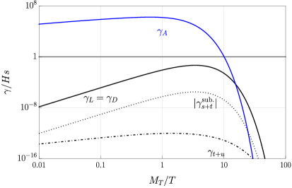
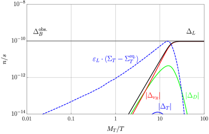
Figure 8: Rate densities (left) for $K=0.01,\;B_{L}=B_{D}=1/2\;\left(Y_{LT}=Y_{TD}=9.1\times 10^{-6}\right),\;\varepsilon_{L}=6.5\times 10^{-4}$ and leptonic yields (right).

We fix $K=0.01\;\text{and}\;B_{L}=B_{D}=1/2$ corresponding to $Y_{LT}=Y_{TD}=9.1\times 10^{-6}$. In the weak washout-regime the gauge annihilations are the last reaction to decouple form thermal equilibrium, as can be seen in the left plot of 8. Since decays and inverse decays are slow, washout will also be slow and the leptonic asymmetry can freeze-in [193] undisturbed. The right figure in 8 illustrates the evolution of the asymmetries: First around $z<1$ equal and opposite amounts of $\Delta_{L}$ and $\Delta_{D}$ are generated. The asymmetries track the deviation of the triplet abundance from equilibrium $\Sigma_{T}-\Sigma_{T}^{\text{eq.}}$. Then the asymmetry in $D$ is transmitted into $\Delta_{\nu_{R}}$ via decays, which is why the corresponding red line starts later at $z\sim 5$. Since the triplet is a Dirac fermion it can develop an asymmetry itself via inverse decays of $\Delta_{L},\Delta_{D}$. Owing to the fact that we take these decays to be slow the resulting $\Delta_{T}$ is small compared to the other asymmetries and the deviation from equilibrium. As the gauge interactions decouple around $z\sim 10$, the triplet abundance does not get restored from here on out and since the out-of-equilibrium decays become faster than the out-of-equilibrium gauge annihilations for $z\sim 20$, the frozen out abundance decays away, explaining the sharp decrease in the triplet abundance $\Sigma_{T}$ at $z\gtrsim 20$. The asymmetry production asymptotes to its final value around this time as there are no more triplets left to decay. After all the triplets and doublets have decayed away only $L$ and $\nu_{R}$ remain. As expected from lepton number conservation we find that the asymptotic values satisfy $\Delta_{L}=-\Delta_{\nu_{R}}$. We stop the evolution at $z=100$ corresponding to $T=M_{T}/100$ long before the sphaleron decoupling because the leptonic asymmetries are conserved after the $T,D$ have decayed. We can reproduce the observed baryon asymmetry today $\Delta_{B}^{\text{obs}}=\eta_{B}/7.04\simeq 10^{-10}$ from (5.26) for an asymmetry parameter of $\varepsilon_{L}=6.5\times 10^{-4}$ corresponding to an efficiency of $\kappa\simeq 2\times 10^{-5}$ from (5.27) in line with our estimate $\kappa\simeq 10^{-4-5}$.

5.6.2 Intermediate Regime

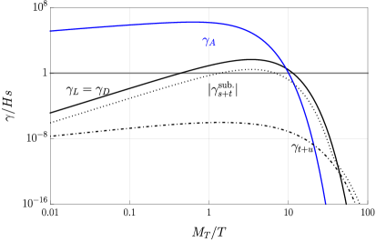
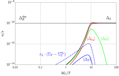
Figure 9: Rate densities (left) for $K=100,\;B_{L}=B_{D}=1/2\;\left(Y_{LT}=Y_{TD}=9.1\times 10^{-4}\right),\;\varepsilon_{L}=2.7\times 10^{-5}$ and leptonic yields (right).

In this regime the decays of the triplet are not negligible during the gauge annihilation phase. Here we fix $K=100\;\text{and}\;B_{L}=B_{D}=1/2$ corresponding to $Y_{LT}=Y_{TD}=9.1\times 10^{-4}$. The evolution of $\Delta_{L}$ is more complicated than in the weak washout-regime owing to the washout from faster inverse decays, which decouple around the same time as the gauge interactions. This is also why a larger $\Delta_{T}$ more comparable to $\varepsilon_{L}\cdot\left(\Sigma_{T}(z)-\Sigma_{T}^{\text{eq.}}(z)\right)$ is generated when compared to the previous benchmark. We fit the observed baryon asymmetry for $\varepsilon_{L}=2.7\times 10^{-5}$ analogous to $\kappa\simeq 4\times 10^{-4}$. This efficiency is indeed larger by an order of magnitude than in the weak washout regime, but not quite as large as our analytical estimate from section 5.4.1.

5.6.3 Strong washout regime

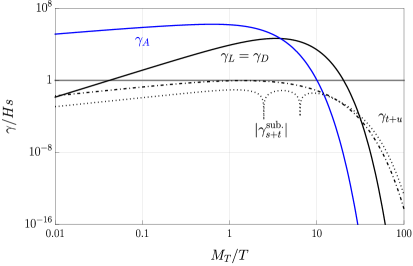
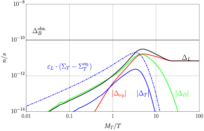
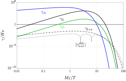
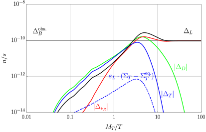
Figure 10: Rate densities (left) for $K=10^{5},\;B_{L}=B_{D}=1/2\;\left(Y_{LT}=Y_{TD}=2.9\times 10^{-2}\right),\;\varepsilon_{L}=3\times 10^{-3}$ and leptonic yields (right).

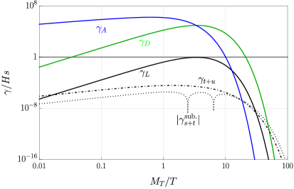
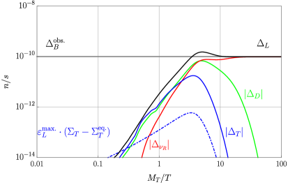
Figure 11: Rate densities (left) for $K=10^{5},\;B_{L}=0.999,\;B_{D}=10^{-3}\;\left(Y_{LT}=4.1\times 10^{-2},\;Y_{TD}=1.2\times 10^{-3}\right),\;\varepsilon_{L}=1.7\times 10^{-3}\sqrt{4B_{L}B_{D}(1-\delta^{2})}=4.7\times 10^{-5}$ and the leptonic yields (right).

Figure 12: Rate densities (left) for $K=10^{5},\;B_{L}=10^{-5},\;B_{D}=0.99999\;\left(Y_{LT}=1.3\times 10^{-4},\;Y_{TD}=4.1\times 10^{-2}\right),\;\varepsilon_{L}=9\times 10^{-5}\sqrt{4B_{L}B_{D}(1-\delta^{2})}=2.2\times 10^{-7}$ and the leptonic yields (right).

For the strong washout regime we fix $K=10^{5}$. In the first scenario we retain $B_{L}=B_{D}=1/2$ which can be realized for $Y_{LT}=Y_{TD}=2.9\times 10^{-2}$. The left plot in 12 shows that indeed the decays are the last interaction to decouple now. Decays and inverse decays are faster than both the annihilations and the Hubble rate only for $z\sim 6-30$. The right plot in the same figure illustrates the evolution of the asymmetries for the maximum possible value of $\varepsilon_{L}=3\times 10^{-3}$ from (5.18). All asymmetries and $\Sigma_{T}-\Sigma_{T}^{\text{eq.}}$ reach their maxima at $z\sim 6$, when the (inverse) decays overtake the gauge annihilations, and decrease afterwards. Once $\gamma_{L}$ decouples at $z\sim 30$ the asymmetry in $\Delta_{L}$ approaches a constant instead of continuing to decrease. This occurs because inverse decays depleting $\Delta_{L}$ are slow now (and eventually there are no more triplets left to decay producing $\Delta_{L}$), analogous to the well known freeze-out scenario for thermal dark matter production. This is in agreement with Sakharov’s conditions [178], since the lepton asymmetry would continue to decrease to zero if the inverse decays depleting them remained in equilibrium forever after $z\sim 6$. Here even for the maximum of $\varepsilon_{L}$ we can not reproduce the observed baryon asymmetry. This happens because of too much washout from inverse decays and as a consequence we have a small efficacy $\kappa\sim 1/K\sim 10^{-5}$. However this is not the end for the strong washout regime. As explained in the previous subsections the larger amount of washout will produce a larger $\Delta_{T}$ and we will make use of this fact to obtain the required efficiency. This behaviour was first observed for decaying scalar triplets in the context of Type II Seesaw leptogenesis [31]. The authors of [31] found that the lepton asymmetry produced by the decay of a non-self-conjugate particle with two decays modes is washed out only if both decay modes are faster than the Hubble rate. Our previous choice $B_{L}=B_{D}$ actually leads to the most amount of washout [31]. We will demonstrate this for two concrete examples:

The first benchmark for the same decay parameter has $B_{L}=0.999\gg B_{D}=10^{-3}$ implying $Y_{LT}=4.1\times 10^{-2},\;Y_{TD}=1.2\times 10^{-3}$. The behavior depicted in the right plot of figure 12 can be understood as follows: First equal and opposite asymmetries in $L,D$ are produced. However since $B_{L}\gg B_{D}$ we find that $\Delta_{L}$ is washed out by the fast inverse decays $LH\rightarrow T$, whereas a large $\Delta_{D}$ develops undisturbed. Of course the asymmetry in $D$ is transmitted to $\nu_{R}$ via the fast decays. The sum rule for lepton number conservation in (5.51) then enforces that

$$\Delta_{D}+\Delta_{\nu_{R}}=-\Delta_{L}-\Delta_{T},$$ (5.53)

which means that the asymmetry in the $D,\nu_{R}$ subsystem is compensated by an equally large asymmetry of opposite sign in the $L,T$ subsystem. When $\Delta_{T}$ eventually decays it gets predominantly transferred to $\Delta_{L}$ again because of $B_{L}\gg B_{D}$. The baryon asymmetry is successfully generated for $\varepsilon_{L}=1.7\times 10^{-3}\sqrt{4B_{L}B_{D}(1-\delta^{2})}=4.7\times 10^{-5}$, where we used a value close to the maximum possible asymmetry of $3\times 10^{-3}$. The difference to the $B_{L}=B_{D}$ case can also be understood if one notices that the triplet asymmetry in 12 is smaller than their deviation from equilibrium $\varepsilon_{L}\cdot\left(\Sigma_{T}(z)-\Sigma_{T}^{\text{eq.}}(z)\right)$. For $B_{L}\gg B_{D}$ on the other hand we can see from 12 that $\Delta_{T}$ actually becomes much larger so that $\Delta_{L}$ starts to track its behaviour.

The second benchmark has $B_{L}=10^{-5}\ll B_{D}=0.99999$ implying $Y_{LT}=1.3\times 10^{-4},\;Y_{TD}=4.1\times 10^{-2}$ and was depicted in figure 12: For $B_{D}\gg B_{L}$ a large initial asymmetry in $L$ can freeze-in and is not washed out. The triplet asymmetry is predominantly produced by inverse decays $DH\rightarrow T$ now. For equal $K$ we find that $\Delta_{T}$ is about an order of magnitude smaller for $B_{D}\gg B_{L}$ compared to $B_{L}\gg B_{D}$, because the inverse decay of $D$ to $T$ has to compete with its fast decay to $\nu_{R}$. Lepton number implies that

$$\Delta_{L}=-\Delta_{D}-\Delta_{\nu_{R}}-\Delta_{T}.$$ (5.54)

When the triplets decay away $\Delta_{T}$ decays primarily to $\Delta_{D}$ because of $B_{D}\gg B_{L}$, and $\Delta_{D}$ decays to $\Delta_{\nu_{R}}$ so again $\Delta_{\nu_{R}}=-\Delta_{L}$ is produced. Note that here we had to rescale $\Sigma_{T}(z)-\Sigma_{T}^{\text{eq.}}(z)$ by the larger $\varepsilon_{L}^{\text{max}}$ and not $\varepsilon_{L}$ to fit it in the same plot with the other yields, since otherwise it would have been smaller than $10^{-14}$. This again illustrates that $\Delta_{T}$ becomes the driving force for this mode instead. This benchmark fits the baryon asymmetry for $\varepsilon_{L}=9\times 10^{-5}\sqrt{4B_{L}B_{D}(1-\delta^{2})}=2.2\times 10^{-7}$. From this we see that the required $\varepsilon_{L}/\sqrt{4B_{L}B_{D}(1-\delta^{2})}$ can be made smaller the more hierarchical the branching ratios $B_{L}/B_{D}$ are.

We conclude by noting that Dirac-Leptogenesis with a decaying fermion naturally realizes all the ingredients needed for the previously mentioned “quasi optimal efficiency”-scenario [31]: Since the decaying fermion is of Dirac nature it can have an asymmetry itself and because of CPT and unitarity (see (5.6)) it needs to have two separate decay modes to generate the leptonic asymmetry parameter. The efficiency increases if their branching ratios are different.

5.7 Lightest neutrino mass

For the previously mentioned benchmarks $M_{T}=10^{8}\;\text{GeV}\;\text{and}\;M_{D}=3\times 10^{7}\;\text{GeV}$ we can use the Yukawa couplings $Y_{LT},Y_{TD}$ required for the different washout scenarios in subsection 5.4.1 to estimate the lightest neutrino mass. The third Yukawa was fixed to $Y_{DR}\simeq 7\times 10^{-4}$ to allow for fast decays of the vector-like doublets see (5.44). Assuming no accidental flavor cancellations we find

$$m_{\nu_{l}} \simeq 5\times 10^{-3}\;\text{eV}\;\cdot Y_{LT}Y_{TD}$$ (5.55)

$$=\begin{cases}6\times 10^{-12}\;\text{eV}\quad\text{for weak washout}\quad Y_{LT}\simeq Y_{TD}\simeq 3.5\times 10^{-5},\\ 5\times 10^{-7}\;\text{eV}\quad\text{for strong washout}\quad Y_{LT}\simeq Y_{TD}\simeq 1.3\times 10^{-2},\end{cases}$$ (5.56)

where the couplings refer only to the lightest doublet and triplet and we assumed equal branching ratios. The lightest neutrino mass eigenstate is substantially lighter than the cosmological limit on the total neutrino mass of $\sum_{\nu}m_{\nu}\lesssim 0.12\;\text{eV}$ [141] and can be treated as massless for all intents and purposes. This outcome is generic in leptogenesis scenarios [194] due to the small couplings required for out of equilibrium decay.

6 Dark radiation

In the SM the number of relativistic neutrinos is found to be [195, 196, 197, 198, 199, 200]

$$N_{\text{eff.}}=3.0440\pm 0.0002,$$ (6.1)

where a small deviation from the value expected for three generations arises as the neutrino decoupling from the SM bath around MeV temperatures is not instantaneous. The abundance of dark radiation is typically parameterized in terms of the effective number of additional neutrinos $\Delta N_{\text{eff.}}$. The value inferred from the observed abundance of light elements produced during Big Bang Nucleosynthesis [141] is

$$N_{\text{eff}}^{\text{BBN}}=2.95^{+0.56}_{-0.52}.$$ (6.2)

Combined analyses of the current Planck CMB data together with Baryon Accoustic oscillations found [141]

$$N_{\text{eff}}^{\text{Planck+BAO}}=2.99^{+0.34}_{-0.33},$$ (6.3)

which can be translated into

$$\Delta N_{\text{eff.}}^{\text{Planck+BAO}}\simeq 0.28.$$ (6.4)

The upcoming CMB Stage IV experiment [201, 202] and NASA’s PICO proposal [203] have a sensitivity forecast of

$$\Delta N_{\text{eff}}^{\text{proj.}}=0.06.$$ (6.5)

There is also the planned CORE experiment by the ESA [204] as well as the South Pole Telescope (SPT) [205] and the Simons observatory [206], which both aim to reach $\Delta N_{\text{eff.}}\lesssim 0.12$.

6.1 Contribution of the axion

The QCD axion does not reach thermal equilibrium via its couplings to the SM leptons: Reactions like $\nu\;\overline{\nu}\leftrightarrow Z\;a$ and $\nu\;e^{+}\leftrightarrow W^{+}\;a$ would only ever thermalize at temperatures far below the $Z$- and $W^{\pm}$-boson masses, because the rates are suppressed with $m_{\nu}^{2}/f_{a}^{2}$. Three body processes like $\nu\;\overline{\nu}\leftrightarrow\nu\;\overline{\nu}\;a$ avoid the production of heavy on-shell EW gauge bosons but are too slow to ever matter due to the previously mentioned tiny couplings. Production of two axions via $\nu\;\overline{\nu}\leftrightarrow a\;a$ is even more suppressed. References [207, 208, 209] showed that the axion decouples from its unavoidable strong interactions with the quark-gluon-plasma at

$$T_{a}^{\text{dec.}}\simeq$1.7\text{\times}{10}^{9}\text{\,}\mathrm{GeV}$\cdot\left(\frac{f_{a}}{10^{11}\;\text{GeV}}\right)^{2.246}.$$ (6.6)

In the HHSI scenario PQ symmetry is broken at $T_{c}\simeq 0.01\;f_{a}$ [12], which occurs after reheating for the typical range of $f_{a}<10^{11}\;\text{GeV}$ and the reheating temperature given by (4.6). Since both the critical temperature and the reheating temperature are larger than the decoupling temperature $T_{a}^{\text{dec.}}$, the axions will have had a thermal abundance in the early universe. Their contribution to the amount of dark radiation can then be estimated to be [12]

$$\Delta N_{\text{eff.}}\simeq 0.027\cdot\left(\frac{100}{g_{*}\left(T_{a}^{\text{dec.}}\right)}\right)^{\frac{4}{3}},$$ (6.7)

which is an order of magnitude below the current bound of (6.4).

6.2 Contribution of the right handed neutrinos

The production of right handed neutrinos is driven by the $Y_{DR}$ Yukawa coupling to the heavy doublet fields $D$ in equation (2.15). Since the doublets have $\text{SU(2)}_{\text{L}}\otimes\text{U(1)}_{\text{Y}}$ gauge interactions they will develop a thermal abundance at high temperatures and can produce $\nu_{R}$ from decays and scattering. Even after the temperature drops below the lightest $D$ mass there are still processes like $H^{\dagger}H\leftrightarrow\overline{\nu_{R}}\nu_{R}$ producing $\nu_{R}$ and keeping them in thermal equilibrium via off-shell $D$-exchange. On dimensional grounds we can estimate the interaction rate for the aforementioned process for $T\gg M_{D}$ as

$$\Gamma(T\gg M_{D})\sim\frac{Y_{DR}^{4}T}{16\pi}$$ (6.8)

and find that it comes into thermal equilibrium at a temperature of

$$T_{\text{coupl.}}\simeq$1.2\text{\times}{10}^{12}\text{\,}\mathrm{GeV}$\cdot\left(\frac{Y_{DR}}{0.1}\right)^{4}\cdot\sqrt{\frac{100}{g_{*}(T_{\text{coupl.}})}}.$$ (6.9)

We therefore expect a thermalized population of $\nu_{R}$ after reheating at around $10^{9}\;\text{GeV}$ (see (4.5)). Since this process is not Boltzmann-suppressed with the heavy $D$-mass it can still be effective until temperatures $T\ll M_{D}$. In this regime we estimate the interaction rate to be

$$\Gamma(T\ll M_{D})\sim\frac{Y_{DR}^{4}}{16\pi M_{D}^{2}}T^{3},$$ (6.10)

where we neglected the Higgs mass and find that it drops out of thermal equilibrium at

$$T_{\text{FO}}\simeq$10\text{\,}\mathrm{TeV}$\cdot\left(\frac{0.1}{Y_{DR}}\right)^{4}\cdot\left(\frac{M_{D}}{${10}^{8}\text{\,}\mathrm{GeV}$}\right)^{2}\cdot\sqrt{\frac{g_{*}(T_{\text{FO}})}{100}}.$$ (6.11)

As this temperature is above the electroweak crossover it was self-consistent to neglect the mass of $H$. For a freeze-out before EWSB we can estimate the contribution of $N_{\nu}$ decoupled $\nu_{R}$ generations to the present day energy density in radiation as [210]

$$\Delta N_{\text{eff}}\simeq 3\;\cdot 0.027\cdot 2\cdot\frac{7}{8}\cdot\left(\frac{100}{g_{*}(T_{\text{FO}})}\right)^{\frac{4}{3}}=0.142.$$ (6.12)

We did not include the predicted asymmetry in $\nu_{R}$ because it is of the order of the small baryon asymmetry and negligible compared to the equilibrium abundance. Together with the contribution from the axion we have $\Delta N_{\text{eff}}\simeq 0.17$ which is allowed by current data see (6.4) and will be probed by next generation experiments. An intriguing way to make our model of Dirac neutrinos compatible with the projected sensitivity (6.5) would be to invoke additional entropy dilution after the decoupling of the right handed neutrinos, which would suppress $\Delta N_{\text{eff}}$ by a factor $\Delta>1$. This mechanism has been used in the past to dilute the overabundance of thermalized keV-scale sterile neutrino dark matter in gauge theories [211, 212] needing $\Delta\sim 100$. Another application of entropy dilution is to bring the gravitino abundance in accordance with the reheating temperature required for vanilla leptogenesis for $\Delta\sim 10^{3}-10^{4}$ [213]. The main ingredient would be a long-lived particle decaying far from equilibrium leading to an intermediate matter dominated epoch [61]. Since this particle needs to decouple while relativistic to produce sufficient entropy it should not have gauge interactions. This leaves only the radial mode of the PQ breaking field $h_{\sigma}$, which could be long-lived via its decays to the SM like Higgs. However the required scalar potential couplings would spoil (4.4) so that inflation and reheating in the HHSI scenario (see section 4.1) would cease to work. Hence we do not consider a long-lived $h_{\sigma}$ further and treat the rather large value of $\Delta N_{\text{eff}}\simeq 0.17$ from the axion and three $\nu_{R}$ as an observational signature to distinguish our scenario from models involving either only a light scalar or only right handed neutrinos.

The smoking gun signature for this model would be observation of such a large $\Delta N_{\text{eff}}$ together with a signal in experiments probing the axion to photon coupling that is enhanced by an order of magnitude compared to the regular QCD axion band (see (2.27)).

7 Summary

• Dirac neutrino masses:
  We constructed Dirac neutrino mass model in the Seesaw spirit, where all heavy particles have masses from the PQ breaking scale and no new scalar besides the PQ breaking singlet is needed. To do so we introduce heavy leptons in the form of electroweak doublets $D$ and triplets $T$. Unlike most models we generate the neutrino masses not via a dimension five operator but rather at dimension six. The only fundamental scales of this model are the EWSB scale $v_{H}$ and the PQ scale $v_{\sigma}$ which can be identified with the axion decay constant $f_{a}$. The lightest Dirac neutrino is approximately massless due to the Yukawa couplings required for leptogenesis.

• Axion to photon coupling:
  Our model involves vector-like fermion that are anomalous with respect to PQ symmetry. They boost the coupling of the QCD axions to a pair of photons by around an order of magnitude (see equation (2.27)) relative to conventional models and can be probed by current experiments such as HAYSTAC, ORGAN and QUAX or future searches by MADMAX, BRASS or ADMX. The new fermions do not lead to phenomenologically relevant Landau Poles for the SM gauge couplings.

• preserving the attractive features of S.M.A.S.H.: The model is compatible with the cosmological history outlined of the original S.M.A.S.H. scenario [11, 12, 13] such as successful inflation, reheating and axion DM from both misalignment and topological defect decay. Our new heavy fermions do not spoil the stability of the scalar potential.

• Dirac-Leptogenesis: We found an alternative for resonant leptogenesis [185] when it comes to enhancing the leptonic asymmetry parameter $\varepsilon_{L}$ in (5.18) by up to six orders of magnitude. Whereas a Majorana triplet fermion needs to have a mass of at least $10^{10}\;\text{GeV}$ our enhanced asymmetry allows for successful leptogenesis even with $10^{8}\;\text{GeV}$ masses. The phenomenology is qualitatively and quantitatively different from the case for Majorana fermions since the triplets can develop asymmetries themselves via washout processes. Choosing different branching ratios for the triplet decays to $L$ and $D$ allows for the “quasi optimal efficiency”-scenario first discussed for decaying scalar triplets in [31]. We identified four parameter regions that reproduce the observed baryon to photon ratio.

• Dark radiation:
  Our setup involves an axion and three right handed neutrinos that were thermalized in the early universe producing a large value of $\Delta N_{\text{eff.}}\simeq 0.17$ which will be probed and potentially excluded by next generation CMB experiments such as CMB-S4, PICO, SPT or the Simons observatory. $\Delta N_{\text{eff.}}$ can be used to distinguish our construction from models involving only a light scalar $(\Delta N_{\text{eff.}}\simeq 0.028)$ like the original S.M.A.S.H. or only right handed neutrinos ($\Delta N_{\text{eff.}}\simeq 0.142$ for three generations).

Appendix A Collection of limits on the axion to photon coupling

Constraints on the axion to photon coupling were compiled in [92] and can be grouped into the following categories

• Haloscopes looking for DM axions from the galactic DM halo
  such as ABRACADABRA [216, 217], ADMX [101, 102, 103, 104, 105, 106, 107, 108], BRASS [109], CAPP [218, 219, 220], DM-Radio [221], HAYSTAC [95, 96], KLASH [222], MADMAX [100], ORGAN [97, 98], QUAX [93, 94], RADES [99], RBF [223], SHAFT [224] and UF [225]

• Helioscopes looking for axions produced inside the sun
  such as CAST [226, 227], babyIAXO or IAXO [228, 229].

• Light shining through walls (LSW) and similar experiments
  such as ALPS [230, 231], CROWS [232], OSQAR [233] and PVLAS [234].

• Cosmological probes
  such as extragalactic background light (EBL), ionisation fraction, X-rays [235] or BBN and $\Delta N_{\text{eff.}}$ [236].

• (indirect) Astrophysical bounds
  such as Black hole superradiance [237], the Chandra X-ray telescope [238, 239, 240, 241], the Fermi Large Area Telescope (LAT) [242, 243, 244, 245], super star clusters [246], the cosmic distance ladder [247], the HESS cherenkov telescope [248], horizontal branch stars [249], White dwarfs [250], Globular Cluster ($R_{2}$) [251], the blazar Markarian 421 (Mark 421) [252], neutron stars [253, 254, 255], observations of the solar neutrino flux [256], supernova SN 1987A [257, 258], radio telescopes [259] and optical telescopes like MUSE [260] and VIMOS [261]

Appendix B Landau poles for the SM gauge couplings

As shown in [59, 60] the hypercharged exotic quarks with masses $5\text{\times}{10}^{11}\text{\,}\mathrm{GeV}$ do not lead to a Landau pole for the $\text{U}_{\text{Y}}$ gauge coupling (or any other SM gauge coupling) below the Planck mass. Following the methods outlined in [110, 111, 91] we compute the coefficients of the two loop renormalization group equations (RGE)

$$\frac{\text{d}}{\text{d}t}\alpha_{i}^{-1}=a_{i}+\frac{b_{ij}}{4\pi}\alpha_{j},\quad\text{where}\quad\alpha_{j}\equiv\frac{g_{j}^{2}}{4\pi}\quad\text{and}\quad t\equiv\frac{1}{2\pi}\text{Log}\left(\frac{\mu}{m_{Z}}\right)$$ (B.1)

where $i=1,2,3$ labels the gauge groups $\text{U}_{\text{Y}}$, $\text{SU(2)}_{\text{L}}$ and $\text{SU(3)}_{\text{c}}$ respectively. Here $\mu$ denotes the renormalization scale. We do not include the contribution from the Yukawa couplings for simplicity. The definitions of the constants can be found in [111, 91] and for the SM they read [110]

$$\vec{a}^{\text{SM}}=\begin{pmatrix}a_{1}\\ a_{2}\\ a_{3}\end{pmatrix}=\begin{pmatrix}4+\frac{1}{10}\\ -22+4+\frac{1}{6}\\ -11+4\end{pmatrix}$$ (B.2)

as well as

$$b^{\text{SM}}=\begin{pmatrix}0&0&0\\ 0&-\frac{132}{3}&0\\ 0&0&-102\end{pmatrix}+N_{\text{gen.}}\begin{pmatrix}\frac{19}{15}&\frac{3}{5}&\frac{44}{15}\\ \frac{1}{5}&\frac{49}{3}&4\\ \frac{11}{30}&\frac{3}{2}&\frac{76}{3}\end{pmatrix}+\begin{pmatrix}\frac{9}{50}&\frac{9}{10}&0\\ \frac{3}{10}&\frac{13}{6}&0\\ 0&0&0\end{pmatrix}.$$ (B.3)

The first matrix comes from the gauge bosons, the second matrix measures the contribution of $N_{\text{gen.}}=3$ generations of fermions and the last matrix arises due to the SM Higgs boson. Note that the matrix $b^{\text{SM}}$ is transposed compared to reference [110] and we used the GUT normalization of SU(5) or SO(10) for the hypercharge [111]

$$Y_{\text{norm.}}=\sqrt{\frac{3}{5}}Y_{\text{SM}}.$$ (B.4)

Motivated by our cosmological findings we only include the lightest electroweak triplet of mass $M_{T}=${10}^{8}\text{\,}\mathrm{GeV}$$ with $Y_{\text{SM}}=0$ for which

$$\vec{a}^{\text{BSM}}_{T}=\begin{pmatrix}0\\ \frac{8}{3}\\ 0\end{pmatrix},\quad b^{\text{BSM}}_{T}=\begin{pmatrix}0&0&0\\ 0&\frac{128}{3}&0\\ 0&0&0\\ \end{pmatrix}$$ (B.5)

and the doublet leptons with $Y_{\text{SM}}=-\frac{1}{2}$ at $M_{D}=$3\text{\times}{10}^{7}\text{\,}\mathrm{GeV}$$ for which

$$\vec{a}^{\text{BSM}}_{D}=\begin{pmatrix}\frac{2}{5}\\ \frac{2}{3}\\ 0\end{pmatrix},\quad b^{\text{BSM}}_{D}=\begin{pmatrix}\frac{9}{50}&\frac{9}{10}&0\\ \frac{3}{10}&\frac{49}{6}&0\\ 0&0&0\\ \end{pmatrix}.$$ (B.6)

We include the threshold effects of the heavy fermions $\Psi$ by solving (B.1) with

$$\vec{a}^{\text{BSM}}=\vec{a}^{\text{SM}}+\Theta\left(\mu-M_{\Psi}\right)\vec{a}_{\Psi}^{\text{BSM}},\quad b^{\text{BSM}}=b^{\text{SM}}+\Theta\left(\mu-M_{\Psi}\right)b_{\Psi}^{\text{BSM}},$$ (B.7)

where $\Theta$ denotes the Heaviside function and we use the following boundary conditions [262, 263]

$$\alpha_{1}(m_{Z})=0.016923,\;\alpha_{2}(m_{Z})=0.03374,\;\alpha_{3}(m_{Z})=0.1173\;\text{and}\;m_{Z}=$91.188\text{\,}\mathrm{GeV}$.$$ (B.8)

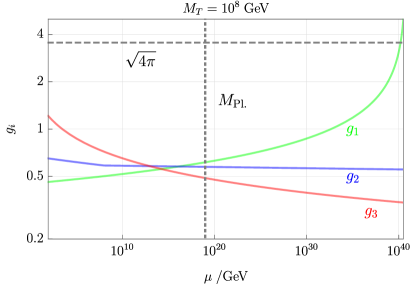
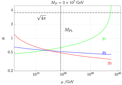
Figure 13: Two Loop RGE evolution of the SM gauge couplings as a function of the renormalization scale for the inclusion of a hypercharge zero $\text{SU}(2)_{\text{L}}$ triplet with $M_{T}=${10}^{8}\text{\,}\mathrm{GeV}$$ (left) and a hypercharge $1/2$ $\text{SU}(2)_{\text{L}}$ doublet fermion with a mass of $M_{D}=$3\text{\times}{10}^{7}\text{\,}\mathrm{GeV}$$ (right).

We reproduce the Landau pole in $g_{1}$ around $10^{38}\;\text{GeV}$ found for a vector-like quark with $Y=-1/3$ with a representative mass of $5\times 10^{11}\;\text{GeV}$ in [59, 60]. We depict the evolution of the three gauge couplings for adding the lightest triplet or doublet in 13 with the masses $M_{T}=10^{8}\;\text{GeV}$ and $M_{D}=3\times 10^{7}\;\text{GeV}$ from section 5.6. One can observe in 13 that the Landau pole appears earlier for the lighter doublet [111]. We stopped the numerical evaluation at the Landau poles because the system of differential equations starts to exhibit singular behaviour and we can not trust our calculation for larger energies anymore. This is why the lines for the doublet in 13 terminate earlier than for the triplet. In both scenarios the potential Landau pole in $g_{1}$ manifests far above the Planck scale, so it does not affect the phenomenology of our model. Let us emphasize that this analysis only serves as a first estimate and in principle all three generations of all new species and their Yukawa interactions should be included in the running. For a more realistic estimate we include three generations of quarks with the same masses of $10^{9}\;\text{GeV}$ for simplicity as well as three generations of triplets, where the two heavier ones have $10^{9}\;\text{GeV}$ masses, together with three doublets, with the two heavier ones at $10^{8}\;\text{GeV}$ (this range of masses was motivated in section 4.3). Adding the entire fermionic particle content of the model induces a Landau pole at $10^{21}\;\text{GeV}$ again in $g_{1}$ and again above the Planck scale. The landau pole appears at lower energies the more fermions we introduce because the positive coefficients in the RGEs (B.1) increase with each additional fermion [59, 60]. We conclude that our three generations of exotic fermions do not lead to phenomenologically relevant Landau Poles for the SM gauge interactions.

Appendix C Sphaleron redistribution coefficient

Once an asymmetry in e.g. the SM leptons is created one has to take into account how this asymmetry is redistributed to the rest of the fermions and the SM Higgs via gauge and Yukawa interactions that are in equilibrium. These fast spectator processes lead to conservation laws for the individual number densities $n_{\psi}$, which for ultra-relativistic fermions (bosons) $\psi$ (and their anti-particles $\overline{\psi}$) can be expressed in terms of their chemical potentials $\mu_{\psi}$ via the relation

$$n_{\psi}-n_{\overline{\psi}}=\frac{\mu_{\psi}g_{\psi}}{3}T^{2}\begin{cases}\frac{1}{2}\quad\text{for fermions}\\ 1\quad\text{for bosons}\end{cases},$$ (C.1)

whereas for a massive particles the appropriate relation would be [264]

$$n_{\psi}-n_{\overline{\psi}}=\frac{\mu_{\psi}g_{\psi}}{\pi^{2}}T^{2}F_{\pm}\left(\frac{m_{\psi}}{T}\right),\quad\text{with}\quad F_{\pm}(x)\equiv\int_{x}^{\infty}\text{d}y\;\frac{y\sqrt{y^{2}-z^{2}}e^{y}}{(1\pm e^{y})^{2}}$$ (C.2)

where the + (-) applies for bosons (fermions). We will work in the regime $T_{\text{EQ}}\simeq\mathcal{O}\left($100\text{\,}\mathrm{GeV}$\right)\ll T<10^{8}\;\text{GeV}$ and since we need to be above the EW phase transition for the sphaleron transition to occur we can work in the regime of unbroken electroweak symmetry where the chemical potential of the gauge bosons is $\mu_{W}=0$ and components of the same multiplet have the same chemical potential [265]. For the SM we include 3 generations of $q,u,d,l,e$ and one Higgs $H$. At temperatures below $10^{8}\;\text{GeV}$ all SM Yukawa interactions are in equilibrium [266] and for simplicity we neglect all flavor effects and assign generation-independent chemical potentials. For the SM the appropriate conditions read [265, 267]

• hypercharge neutrality of the plasma

  $$3\left(\mu_{q}+2\mu_{u}-\mu_{d}-\mu_{l}-\mu_{e}\right)+2\mu_{H}=0$$ (C.3)

• $\text{SU}(2)_{\text{L}}$ sphalerons

  $$3\mu_{q}+\mu_{l}=0\quad\text{from}\quad\mathcal{O}_{\text{sph.}}=\Pi_{i=1}^{3}l_{i}q_{i}q_{i}q_{i}$$ (C.4)

• $\text{SU}(3)_{\text{c}}$ sphalerons

  $$2\mu_{q}-\mu-\mu_{d}=0$$ (C.5)

• SM Yukawa interactions

  $$\mu_{l}-\mu_{H}-\mu_{e} =0\quad\text{from}\quad\overline{L}He,$$ (C.6)

  $$\mu_{q}-\mu_{H}-\mu_{d} =0\quad\text{from}\quad\overline{Q}Hd,$$ (C.7)

  $$\mu_{q}+\mu_{H}-\mu_{u} =0\quad\text{from}\quad\overline{Q}\tilde{H}u.$$ (C.8)

Note that since all Yukawa interactions equilibrate the $\text{SU}(3)_{\text{c}}$ sphaleron condition (C.5) becomes redundant as it is jus the sum of (C.7) and (C.8). As we have six potentials and only five conditions we can express five chemcial potentials in terms of a sixth. We choose the potential for the total baryon minus lepton number for three generations in the SM

$$\mu_{\text{B}-\text{L}_{\text{SM}}}=2\mu_{q}+\mu_{u}+\mu_{d}-2\mu_{l}-\mu_{e},$$ (C.9)

because it is not washed put by the weak sphalerons and recover the famous relations

$$\mu_{\text{B}}=\frac{28}{79}\mu_{\text{B}-\text{L}_{\text{SM}}},\quad\mu_{\text{L}_{\text{SM}}}=-\frac{51}{79}\mu_{\text{B}-\text{L}_{\text{SM}}}.$$ (C.10)

Next we add the additional BSM particles. We start with three gauge singlets $\nu_{R}$. The previous conditions are unchanged, but since our theory conserves B-L we have to impose this on the potentials

$$\mu_{\text{B}-\text{L}_{\text{tot}}}=\mu_{\text{B}-\text{L}_{\text{SM}}}-\mu_{\nu_{R}}=0,$$ (C.11)

which by itself would lead to [162]

$$\mu_{\text{B}}=\mu_{\text{L}_{\text{tot}}}=\frac{28}{79}\mu_{\text{B}-\text{L}_{\text{SM}}}.$$ (C.12)

However we also add the lightest two vector-like doublets $(D_{L},D_{R})$ with $Y=1/2$ and lepton number 1. The heavier doublets will be Boltzmann suppressed. We assume that the interaction $\sigma\overline{D_{L}}D_{R}$ was in equilibrium at high temperatures and since after Peccei-Quinn breaking we have $\mu_{\sigma}=0$ we conclude that $\mu_{D_{L}}=\mu_{D_{R}}\equiv\mu_{D}$. The hypercharge neutrality condition is modified to

$$3\left(\mu_{q}+2\mu_{u}-\mu_{d}-\mu_{l}-\mu_{e}\right)+2\mu_{H}+2\mu_{D}=0,$$ (C.13)

where the factor of two for $\mu_{H}$ appears because the scalar Higgs has different quantum statistics compared to the fermions and the factor two for $\mu_{D}$ appears because of the two chiralities we add. We furthermore demand that their coupling to $\nu_{R}$ is in equilibrium so that there is no population of stable heavy leptons (see section 5.4.2)

$$\mu_{D}-\mu_{H}-\mu_{\nu_{R}}=0\quad\text{from}\quad\overline{D_{L}}H\nu_{R}.$$ (C.14)

Since the $D$s are leptonic doublets we expect them to couple to the weak sphaleron transition. Naively one would expect to replace $\mu_{l}$ the condition (C.4) with $-\mu_{D}$, because of the opposite hypercharge. However the pair of vector-like fermions $(D_{L},D_{R})$ does not contribute to the $\text{U}(1)_{\text{B+L}}\otimes\text{SU}(2)_{\text{L}}^{2}$ anomaly. Reference [179] computed the effective sphaleron mediated operators and since the vector-like leptons do not lead to B+L violation the modified sphaleron vertex will still correspond to a $\Delta\left(\text{B+L}\right)=6$ transition like the original in (C.4) and only involves a pair of vector-like leptons

$$\mathcal{O}_{\text{sph. I}}^{\text{SM}+\text{VL}}=\left(\Pi_{i=1}^{3}l_{i}q_{i}q_{i}q_{i}\right)D_{L}\overline{D_{R}}.$$ (C.15)

One can see that this vertex does not lead to new constraints on the chemical potential and that the asymmetry in $D$ can not be converted into a baryonic asymmetry. Let us continue with the conservation of the total B-L

$$\mu_{\text{B}-\text{L}_{\text{tot}}}=\mu_{\text{B}-\text{L}_{\text{SM}}}-\mu_{\nu_{R}}-\frac{4}{3}\mu_{D}=0,$$ (C.16)

where the factor of $4/3$ arises because of the two doublets $D_{L,R}$ and there is only one generation of heavy doublets in the plasma compared to the three generations of the SM quarks, leptons and $\nu_{R}$. Moreover the Boltzmann equations in section 5.5 respect the conservation of total lepton number see (5.51) as well. Solving the system of equations of (C.13),(C.14) and (C.16) together with the previously mentioned conditions on the SM chemical potentials we arrive at

$$\mu_{\text{B}}=\mu_{\text{L}_{\text{tot}}}=\frac{55}{148}\mu_{\text{B}-\text{L}_{\text{SM}}},\quad\mu_{D}=\frac{201}{592}\mu_{\text{B}-\text{L}_{\text{SM}}}\quad\text{and}\quad\mu_{\nu_{R}}=\frac{81}{148}\mu_{\text{B}-\text{L}_{\text{SM}}}.$$ (C.17)

The conversion factor for generating B from $\text{B}-\text{L}_{\text{SM}}$ of $55/148\simeq 0.37$ is only slightly larger than the SM result $28/79\simeq 0.35$.

Appendix D Cross sections and rate densities

The relevant cross sections are given in terms of the following dimensionless variables

$$\delta\equiv\left(\frac{M_{D}}{M_{T}}\right)^{2},\quad x\equiv\frac{s}{M_{T}^{2}},\quad r\equiv\sqrt{1-\frac{4}{x}},\quad\omega\equiv\frac{\Gamma_{\text{tot.}}}{M_{T}}$$ (D.1)

and read

• process $L\overline{D}\rightarrow HH$ possible in the $t-$ and $u$-channel:

  $$\sigma_{t+u} =\frac{3}{8\pi M_{T}^{2}}\left(\frac{x-\delta}{x^{2}(1+x-\delta)}-\frac{\text{Log}(1+x-\delta)}{x^{2}(2+x-\delta)}\right)$$ (D.2)

  $$=\frac{3}{8\pi}\begin{cases}\frac{1}{2M_{T}^{2}}\quad\text{for}\;s\ll M_{T}^{2}\\ \frac{1}{s}\quad\text{for}\;s\gg M_{T}^{2}\end{cases}$$ (D.3)

• subtracted cross section (see section 5.5) for the process $LH\rightarrow DH$ possible in the $s-$ and $t-$channel:

  $$\sigma_{s+t}^{\text{sub.}} =\frac{M_{T}^{2}}{32\pi x^{2}}(x^{2}-\delta^{2})\sum^{3}_{a=1}\left|D_{s}^{a}(s)\right|^{\text{sub.}\,\;2}$$ (D.4)

  $$+\frac{3}{16\pi M_{T}^{2}x^{2}}\frac{(x-\delta)((x-1)(-2+(x-1)x+\delta)+(1+x)\omega^{2})}{(1+x-\delta)((x-1)^{2}+\omega^{2})}$$

  $$+\frac{3}{16\pi M_{T}^{2}x^{2}}\frac{(-2+2x+\omega^{2})\text{Log}(1+x-\delta)}{(1-x)^{2}+\omega^{2}}$$

  $$=\frac{3}{16\pi}\begin{cases}\frac{1}{2M_{T}^{2}}\quad\text{for}\;s\ll M_{T}^{2}\\ \frac{1}{s}\quad\text{for}\;s\gg M_{T}^{2}\end{cases}$$ (D.5)

  where for all $a=1,2,3$

  $$\left|D_{s}^{a}(s)\right|^{\text{sub.}\,\;2}\equiv\left|\frac{1}{s-M_{T}^{2}+iM_{T}\Gamma_{\text{tot.}}}\right|^{2}-\frac{\pi\delta(s-M_{T}^{2})}{M_{T}\Gamma_{\text{tot.}}}.$$ (D.6)

  For the numerical evaluation it is convenient to carry out the thermal average of the subtracted matrix element (5.47) rather than to subtract the densities appearing in (5.46). We follow the methods of [186] and use the following representation of the $\delta$-distribution which decreases faster than the propagator away from the resonance

  $$\delta(y)=\frac{2\rho^{3}}{\pi\left(y^{2}+\rho^{2}\right)}\quad\text{with}\quad y=\frac{s}{M_{T}^{2}}-1,$$ (D.7)

  where $\rho\ll 1$. Since we find $\Gamma_{\text{tot.}}/M_{T}<10^{-5}$ we are always in the narrow width regime and may set $\rho=\Gamma_{\text{tot.}}/M_{T}$ [186].

• process $T\overline{T}\rightarrow WW,F\overline{F}$, where $W$ are the $\text{SU}(2)_{\text{L}}$ gauge bosons and $F$ represents the SM fermion doublets [182]:

  $$\sigma_{W} =\frac{g_{2}^{4}}{\pi M_{T}^{2}x\;r^{2}}\left(3r\left(1+\frac{2}{x}\right)-r\left(4+\frac{17}{x}\right)\right)$$ (D.8)

  $$+\frac{3g_{2}^{4}}{\pi M_{T}^{2}x\;r^{2}}\left(1+\frac{4}{x}-\frac{4}{x^{2}}\right)\text{Log}\left(\frac{1+r}{1-r}\right)$$

  For non-relativistic triplets the gauge scattering rate density can be approximately written as [268, 269]

  $$\gamma\left(T\;\overline{T}\leftrightarrow WW,F\overline{F}\right)=4\times\frac{M_{T}T^{3}}{32\pi^{3}}e^{-2\frac{M_{T}}{T}}\left(c_{s}+3\frac{T}{M_{T}}\left(c_{p}+c_{s}\right)+\mathcal{O}\left(\frac{T^{2}}{M_{T}^{2}}\right)\right),$$ (D.9)

  where we inserted a factor of four by hand to take into account that Dirac triplets have twice as many internal degrees of freedom as Majorana ones (see (E.3)). Furthermore

  $$c_{s}=\frac{111}{8\pi}g_{2}^{4}\quad\text{and}\quad c_{p}=\frac{51}{8\pi}g_{2}^{4}$$ (D.10)

  are the $s$- and $p$-wave coefficients from the non-relativistic velocity expansion.

Appendix E CP-violating rate densities

$\gamma_{\text{tot}}$ is the thermal average of $\Gamma_{\text{tot}}$ in equation (5.5) computed via [186]

$$\gamma\left(\psi\rightarrow\dots\right)=\left(n_{\psi}^{\text{eq.}}+n_{\overline{\psi}}^{\text{eq.}}\right)\frac{K_{1}(z)}{K_{2}(z)}\Gamma\left(\psi\rightarrow\dots\right)$$ (E.1)

where we introduced $z\equiv m_{\psi}/T$ and $\text{K}_{1,2}(z)$ denotes the special Bessel functions of the first and second kind. The equilibrium number density of a particle $\psi$ reads [270]

$$n_{\psi}^{\text{eq.}}(z)=g_{\psi}\frac{T^{3}}{\pi^{2}}\begin{cases}\zeta(3)\quad\text{for bosons with}\quad T\gg m_{\psi},\\ \frac{3}{4}\zeta(3)\quad\text{for fermions with}\quad T\gg m_{\psi},\\ \frac{z^{2}\text{K}_{2}(z)}{2}\quad\text{for}\quad T\ll m_{\psi},\end{cases}$$ (E.2)

with $g_{\psi}$ being the spin degeneracy of $\psi$. For scattering processes with a cross section $\sigma$ the appropriate thermally averaged density in the Maxwell-Boltzmann approximation is found to be [271, 270]

$$\gamma\left(a+b\leftrightarrow i+j+\dots\right)=g_{a}g_{b}\frac{T}{32\pi^{4}}\int_{s_{\text{min}}}^{\infty}\text{d}s\;s^{\frac{3}{2}}\lambda\left(1,\frac{m_{a}^{2}}{s},\frac{m_{b}^{2}}{s}\right)K_{1}\left(\frac{\sqrt{s}}{T}\right)\;\sigma,\quad$$ (E.3)

with $g_{a,b}$ denoting the spin degeneracies of particles $a,b$ and

$$\lambda(a,b,c)\equiv(a-b-c)^{2}-4bc$$ (E.4)

together with $s_{\text{min}}=\text{max}\left[\left(m_{a}+m_{b}\right)^{2},\left(m_{i}+m_{j}+\dots\right)^{2}\right]$. We parameterize the CP-violating thermally averaged decay widths in the following way [31]

$$\gamma_{\text{eq.}}\left(T\rightarrow LH\right) = \gamma_{\text{eq.}}\left(\overline{L}H^{\dagger}\rightarrow\overline{T}\right)=\left(\text{B}_{\text{L}}+\varepsilon_{L}\right)\gamma_{\text{tot}}$$ (E.5)

$$\gamma_{\text{eq.}}\left(\overline{T}\rightarrow\overline{L}H^{\dagger}\right) = \gamma_{\text{eq.}}\left(LH\rightarrow T\right)=\left(\text{B}_{\text{L}}-\varepsilon_{L}\right)\gamma_{\text{tot}}$$ (E.6)

$$\gamma_{\text{eq.}}\left(T\rightarrow DH\right) = \gamma_{\text{eq.}}\left(\overline{D}H^{\dagger}\rightarrow\overline{T}\right)=\left(\text{B}_{\text{D}}-\varepsilon_{L}\right)\gamma_{\text{tot}}$$ (E.7)

$$\gamma_{\text{eq.}}\left(\overline{T}\rightarrow\overline{D}H^{\dagger}\right) = \gamma_{\text{eq.}}\left(DH\rightarrow T\right)=\left(\text{B}_{\text{D}}+\varepsilon_{L}\right)\gamma_{\text{tot}}$$ (E.8)

which follows from CPT invariance and the definition of $\varepsilon$. The CP conserving branching ratios of the decay widths are defined in (5.4). Furthermore the same branching ratios apply to the CP conserving part of $\gamma_{\text{eq.}}/\gamma_{\text{tot.}}$ because the factors from the thermal averages divide out. Washout scattering mediated by $T$ occurs at the same order in the perturbative expansion as the generation of $\varepsilon$. The washout rate can be decomposed into two contributions $\gamma_{T_{s+t}}$ and $\gamma_{T_{t+u}}$. Because of CPT invariance the rate densities for the following reactions only possible in the $t$- and $u$-channel have to satisfy

$$\gamma\left(L\overline{D}\rightarrow HH\right)=\gamma\left(H^{\dagger}H^{\dagger}\rightarrow\overline{L}D\right)\equiv\gamma_{T_{t+u}}$$ (E.9)

and the reactions possible in both the $s$- and $t$-channel satisfy

$$\gamma\left(\overline{D}H^{\dagger}\rightarrow\overline{L}H^{\dagger}\right) = \gamma\left(LH\rightarrow DH\right),$$ (E.10)

$$\gamma\left(DH\rightarrow LH\right) = \gamma\left(\overline{L}H^{\dagger}\rightarrow\overline{D}H^{\dagger}\right).$$ (E.11)

Here the $s$-channel contribution to the washout scattering $\gamma_{T_{s+t}}$ involves intermediate on shell $T$s whose decays and inverse decays are already accounted for in the Boltzmann equation. Therefore we have to perform real intermediate state (RIS) subtraction to remove the on shell contribution [192, 186, 272] which can be expressed as [186]

$$\gamma\left(LH\rightarrow DH\right)_{\text{eq.}} = \gamma_{T_{s+t}}-\gamma_{\text{eq.}}\left(LH\rightarrow T\right)\text{BR}\left(T\rightarrow DH\right),$$ (E.12)

$$\gamma\left(\overline{L}H^{\dagger}\rightarrow\overline{D}H^{\dagger}\right)_{\text{eq.}} = \gamma_{T_{s+t}}-\gamma_{\text{eq.}}\left(\overline{L}H^{\dagger}\rightarrow\overline{T}\right)\text{BR}\left(\overline{T}\rightarrow\overline{D}H^{\dagger}\right),$$ (E.13)

and we expand the CP violating branching ratios in the subtracted rates to leading order in $\varepsilon_{L}$:

$$\gamma\left(LH\rightarrow DH\right)_{\text{eq.}} = \gamma_{T_{s+t}}-B_{L}B_{D}\gamma_{\text{tot.}}+\varepsilon_{L}\;\gamma_{\text{tot.}}+\mathcal{O}\left(\varepsilon_{L}^{2}\right)$$ (E.14)

$$\gamma\left(\overline{L}H^{\dagger}\rightarrow\overline{D}H^{\dagger}\right)_{\text{eq.}} = \gamma_{T_{s+t}}-B_{L}B_{D}\gamma_{\text{tot.}}-\varepsilon_{L}\;\gamma_{\text{tot.}}+\mathcal{O}\left(\varepsilon_{L}^{2}\right)$$ (E.15)

Due to these relations we define the following object [31]

$$\gamma_{T_{s+t}}^{\text{sub.}}=\gamma_{T_{s+t}}-B_{L}B_{D}\gamma_{\text{tot.}}$$ (E.16)

References

- [1] Peter Minkowski. at a Rate of One Out of Muon Decays? Phys. Lett. B, 67:421–428, 1977.
- [2] Tsutomu Yanagida. Horizontal gauge symmetry and masses of neutrinos. Conf. Proc. C, 7902131:95–99, 1979.
- [3] Murray Gell-Mann, Pierre Ramond, and Richard Slansky. Complex Spinors and Unified Theories. Conf. Proc. C, 790927:315–321, 1979.
- [4] S. L. Glashow. The Future of Elementary Particle Physics. NATO Sci. Ser. B, 61:687, 1980.
- [5] Tsutomu Yanagida. Horizontal Symmetry and Masses of Neutrinos. Progress of Theoretical Physics, 64(3):1103–1105, 09 1980.
- [6] Rabindra N. Mohapatra and Goran Senjanović. Neutrino mass and spontaneous parity nonconservation. Phys. Rev. Lett., 44:912–915, Apr 1980.
- [7] M. Fukugita and T. Yanagida. Barygenesis without grand unification. Physics Letters B, 174(1):45–47, 1986.
- [8] Takehiko Asaka, Steve Blanchet, and Mikhail Shaposhnikov. The nuMSM, dark matter and neutrino masses. Phys. Lett. B, 631:151–156, 2005.
- [9] Takehiko Asaka and Mikhail Shaposhnikov. The MSM, dark matter and baryon asymmetry of the universe. Phys. Lett. B, 620:17–26, 2005.
- [10] Mikhail Shaposhnikov and Igor Tkachev. The nuMSM, inflation, and dark matter. Phys. Lett. B, 639:414–417, 2006.
- [11] Guillermo Ballesteros, Javier Redondo, Andreas Ringwald, and Carlos Tamarit. Unifying inflation with the axion, dark matter, baryogenesis and the seesaw mechanism. Phys. Rev. Lett., 118(7):071802, 2017.
- [12] Guillermo Ballesteros, Javier Redondo, Andreas Ringwald, and Carlos Tamarit. Standard Model—axion—seesaw—Higgs portal inflation. Five problems of particle physics and cosmology solved in one stroke. JCAP, 08:001, 2017.
- [13] Guillermo Ballesteros, Javier Redondo, Andreas Ringwald, and Carlos Tamarit. Several Problems in Particle Physics and Cosmology Solved in One SMASH. Front. Astron. Space Sci., 6:55, 2019.
- [14] Michael Shin. Light Neutrino Masses and Strong CP Problem. Phys. Rev. Lett., 59:2515, 1987. [Erratum: Phys.Rev.Lett. 60, 383 (1988)].
- [15] Jihn E. Kim. Weak-interaction singlet and strong invariance. Phys. Rev. Lett., 43:103–107, Jul 1979.
- [16] M.A. Shifman, A.I. Vainshtein, and V.I. Zakharov. Can confinement ensure natural cp invariance of strong interactions? Nuclear Physics B, 166(3):493–506, 1980.
- [17] Alberto Salvio. A Simple Motivated Completion of the Standard Model below the Planck Scale: Axions and Right-Handed Neutrinos. Phys. Lett. B, 743:428–434, 2015.
- [18] A. R. Zhitnitsky. On Possible Suppression of the Axion Hadron Interactions. (In Russian). Sov. J. Nucl. Phys., 31:260, 1980.
- [19] Michael Dine, Willy Fischler, and Mark Srednicki. A simple solution to the strong cp problem with a harmless axion. Physics Letters B, 104(3):199–202, 1981.
- [20] Alexei H. Sopov and Raymond R. Volkas. VISH: a unified solution to five SM shortcomings with a protected electroweak scale. 2206.11598, 6 2022.
- [21] Ernest Ma and Rahul Srivastava. Dirac or inverse seesaw neutrino masses with gauge symmetry and flavor symmetry. Phys. Lett. B, 741:217–222, 2015.
- [22] Ernest Ma, Nicholas Pollard, Rahul Srivastava, and Mohammadreza Zakeri. Gauge Model with Residual Symmetry. Phys. Lett. B, 750:135–138, 2015.
- [23] Ernest Ma and Rahul Srivastava. Dirac or inverse seesaw neutrino masses from gauged symmetry. Mod. Phys. Lett. A, 30(26):1530020, 2015.
- [24] Ernest Ma. and Seesaw Dirac Neutrinos. Letters in High Energy Physics, 11 2018.
- [25] Pei-Hong Gu and Utpal Sarkar. Radiative Neutrino Mass, Dark Matter and Leptogenesis. Phys. Rev. D, 77:105031, 2008.
- [26] Yasaman Farzan and Ernest Ma. Dirac neutrino mass generation from dark matter. Phys. Rev. D, 86:033007, 2012.
- [27] Salvador Centelles Chuliá, Ernest Ma, Rahul Srivastava, and José W. F. Valle. Dirac Neutrinos and Dark Matter Stability from Lepton Quarticity. Phys. Lett. B, 767:209–213, 2017.
- [28] Salvador Centelles Chuliá, Rahul Srivastava, and José W. F. Valle. Seesaw roadmap to neutrino mass and dark matter. Phys. Lett. B, 781:122–128, 2018.
- [29] Salvador Centelles Chuliá, Rahul Srivastava, and José W. F. Valle. Seesaw Dirac neutrino mass through dimension-six operators. Phys. Rev. D, 98(3):035009, 2018.
- [30] Salvador Centelles Chuliá, Ricardo Cepedello, Eduardo Peinado, and Rahul Srivastava. Systematic classification of two loop = 4 Dirac neutrino mass models and the Diracness-dark matter stability connection. JHEP, 10:093, 2019.
- [31] Thomas Hambye, Martti Raidal, and Alessandro Strumia. Efficiency and maximal CP-asymmetry of scalar triplet leptogenesis. Phys. Lett. B, 632:667–674, 2006.
- [32] M. Roncadelli and D. Wyler. Naturally light dirac neutrinos in gauge theories. Physics Letters B, 133(5):325–329, 1983.
- [33] Steven Weinberg. Baryon- and lepton-nonconserving processes. Phys. Rev. Lett., 43:1566–1570, Nov 1979.
- [34] Eduardo Peinado, Mario Reig, Rahul Srivastava, and Jose W. F. Valle. Dirac neutrinos from Peccei–Quinn symmetry: A fresh look at the axion. Mod. Phys. Lett. A, 35(21):2050176, 2020.
- [35] R. D. Peccei and Helen R. Quinn. conservation in the presence of pseudoparticles. Phys. Rev. Lett., 38:1440–1443, Jun 1977.
- [36] R. D. Peccei and Helen R. Quinn. Constraints Imposed by CP Conservation in the Presence of Instantons. Phys. Rev. D, 16:1791–1797, 1977.
- [37] Kazuo Fujikawa. On the Evaluation of Chiral Anomaly in Gauge Theories with Gamma(5) Couplings. Phys. Rev. D, 29:285, 1984.
- [38] Luca Di Luzio, Maurizio Giannotti, Enrico Nardi, and Luca Visinelli. The landscape of QCD axion models. Phys. Rept., 870:1–117, 2020.
- [39] Alexander Vilenkin and Allen E. Everett. Cosmic strings and domain walls in models with goldstone and pseudo-goldstone bosons. Phys. Rev. Lett., 48:1867–1870, Jun 1982.
- [40] Alexander Vilenkin. Cosmic strings and domain walls. Physics Reports, 121(5):263–315, 1985.
- [41] A. Vilenkin and E. P. S. Shellard. Cosmic Strings and Other Topological Defects. Cambridge University Press, 7 2000.
- [42] William H Press. Spontaneous production of the zel'dovich spectrum of cosmological fluctuations. Physica Scripta, 21(5):702–707, jan 1980.
- [43] P. Sikivie. Axions, domain walls, and the early universe. Phys. Rev. Lett., 48:1156–1159, Apr 1982.
- [44] T W B Kibble. Topology of cosmic domains and strings. Journal of Physics A: Mathematical and General, 9(8):1387–1398, aug 1976.
- [45] T. W. B. Kibble, G. Lazarides, and Q. Shafi. Walls bounded by strings. Phys. Rev. D, 26:435–439, Jul 1982.
- [46] T.W.B. Kibble. Some implications of a cosmological phase transition. Physics Reports, 67(1):183–199, 1980.
- [47] Alexander Vilenkin. Cosmic strings. Phys. Rev. D, 24:2082–2089, Oct 1981.
- [48] R.L. Davis. Cosmic axions from cosmic strings. Physics Letters B, 180(3):225–230, 1986.
- [49] Takashi Hiramatsu, Masahiro Kawasaki, Ken’ichi Saikawa, and Toyokazu Sekiguchi. Production of dark matter axions from collapse of string-wall systems. Phys. Rev. D, 85:105020, 2012. [Erratum: Phys.Rev.D 86, 089902 (2012)].
- [50] Marco Gorghetto, Edward Hardy, and Giovanni Villadoro. Axions from Strings: the Attractive Solution. JHEP, 07:151, 2018.
- [51] Alejandro Vaquero, Javier Redondo, and Julia Stadler. Early seeds of axion miniclusters. Journal of Cosmology and Astroparticle Physics, 2019(04):012–012, apr 2019.
- [52] S. M. Barr and Jihn E. Kim. New confining force solution of the qcd axion domain-wall problem. Phys. Rev. Lett., 113:241301, Dec 2014.
- [53] Mario Reig. On the high-scale instanton interference effect: axion models without domain wall problem. JHEP, 08:167, 2019.
- [54] Andrea Caputo and Mario Reig. Cosmic implications of a low-scale solution to the axion domain wall problem. Phys. Rev. D, 100(6):063530, 2019.
- [55] Pierre Sikivie. Axion Cosmology. Lect. Notes Phys., 741:19–50, 2008.
- [56] Masahiro Kawasaki and Kazunori Nakayama. Axions: Theory and Cosmological Role. Ann. Rev. Nucl. Part. Sci., 63:69–95, 2013.
- [57] G. Lazarides and Q. Shafi. Axion models with no domain wall problem. Physics Letters B, 115(1):21–25, 1982.
- [58] S.M. Barr, D.B. Reiss, and A. Zee. Families, the invisible axion, and domain walls. Physics Letters B, 116(4):227–230, 1982.
- [59] Luca Di Luzio, Federico Mescia, and Enrico Nardi. Redefining the Axion Window. Phys. Rev. Lett., 118(3):031801, 2017.
- [60] Luca Di Luzio, Federico Mescia, and Enrico Nardi. Window for preferred axion models. Phys. Rev. D, 96(7):075003, 2017.
- [61] Robert J. Scherrer and Michael S. Turner. Decaying Particles Do Not Heat Up the Universe. Phys. Rev. D, 31:681, 1985.
- [62] Albert M Sirunyan et al. Search for vector-like T and B quark pairs in final states with leptons at 13 TeV. JHEP, 08:177, 2018.
- [63] Morad Aaboud et al. Combination of the searches for pair-produced vector-like partners of the third-generation quarks at 13 TeV with the ATLAS detector. Phys. Rev. Lett., 121(21):211801, 2018.
- [64] Rabindra N. Mohapatra. Mechanism for understanding small neutrino mass in superstring theories. Phys. Rev. Lett., 56:561–563, Feb 1986.
- [65] R. N. Mohapatra and J. W. F. Valle. Neutrino mass and baryon-number nonconservation in superstring models. Phys. Rev. D, 34:1642–1645, Sep 1986.
- [66] Sidney Coleman. Why there is nothing rather than something: A theory of the cosmological constant. Nuclear Physics B, 310(3):643–668, 1988.
- [67] Steven B. Giddings and Andrew Strominger. Loss of incoherence and determination of coupling constants in quantum gravity. Nuclear Physics B, 307(4):854–866, 1988.
- [68] Gerald Gilbert. Wormhole-induced proton decay. Nuclear Physics B, 328(1):159–170, 1989.
- [69] Renata Kallosh, Andrei D. Linde, Dmitri A. Linde, and Leonard Susskind. Gravity and global symmetries. Phys. Rev. D, 52:912–935, 1995.
- [70] Rodrigo Alonso and Alfredo Urbano. Wormholes and masses for Goldstone bosons. JHEP, 02:136, 2019.
- [71] Howard M. Georgi, Lawrence J. Hall, and Mark B. Wise. Grand unified models with an automatic peccei-quinn symmetry. Nuclear Physics B, 192(2):409–416, 1981.
- [72] Michael Dine and Nathan Seiberg. String theory and the strong cp problem. Nuclear Physics B, 273(1):109–124, 1986.
- [73] S. M. Barr and D. Seckel. Planck-scale corrections to axion models. Phys. Rev. D, 46:539–549, Jul 1992.
- [74] Marc Kamionkowski and John March-Russell. Planck-scale physics and the peccei-quinn mechanism. Physics Letters B, 282(1):137–141, 1992.
- [75] Richard Holman, Stephen D. H. Hsu, Thomas W. Kephart, Edward W. Kolb, Richard Watkins, and Lawrence M. Widrow. Solutions to the strong CP problem in a world with gravity. Phys. Lett. B, 282:132–136, 1992.
- [76] S. Ghigna, M. Lusignoli, and M. Roncadelli. Instability of the invisible axion. Physics Letters B, 283(3):278–281, 1992.
- [77] Andre de Gouvea and J. W. F. Valle. Minimalistic neutrino mass model. Phys. Lett. B, 501:115–127, 2001.
- [78] J. T. Penedo, Yakefu Reyimuaji, and Xinyi Zhang. Axionic Dirac seesaw and electroweak vacuum stability. 2208.03329, 8 2022.
- [79] Steven Weinberg. A new light boson? Phys. Rev. Lett., 40:223–226, Jan 1978.
- [80] F. Wilczek. Problem of strong and invariance in the presence of instantons. Phys. Rev. Lett., 40:279–282, Jan 1978.
- [81] William A. Bardeen, R. D. Peccei, and T. Yanagida. CONSTRAINTS ON VARIANT AXION MODELS. Nucl. Phys. B, 279:401–428, 1987.
- [82] David B. Kaplan. Opening the axion window. Nuclear Physics B, 260(1):215–226, 1985.
- [83] Mark Srednicki. Axion Couplings to Matter. 1. CP Conserving Parts. Nucl. Phys. B, 260:689–700, 1985.
- [84] Marco Farina, Duccio Pappadopulo, Fabrizio Rompineve, and Andrea Tesi. The photo-philic QCD axion. JHEP, 01:095, 2017.
- [85] Tetsutaro Higaki, Kwang Sik Jeong, Naoya Kitajima, and Fuminobu Takahashi. The QCD Axion from Aligned Axions and Diphoton Excess. Phys. Lett. B, 755:13–16, 2016.
- [86] Tetsutaro Higaki, Kwang Sik Jeong, Naoya Kitajima, and Fuminobu Takahashi. Quality of the Peccei-Quinn symmetry in the Aligned QCD Axion and Cosmological Implications. JHEP, 06:150, 2016.
- [87] Anton V. Sokolov and Andreas Ringwald. Photophilic hadronic axion from heavy magnetic monopoles. JHEP, 06:123, 2021.
- [88] Anton V. Sokolov and Andreas Ringwald. Electromagnetic Couplings of Axions. 2205.02605, 5 2022.
- [89] Anson Hook. Solving the Hierarchy Problem Discretely. Phys. Rev. Lett., 120(26):261802, 2018.
- [90] Luca Di Luzio, Belen Gavela, Pablo Quilez, and Andreas Ringwald. An even lighter QCD axion. JHEP, 05:184, 2021.
- [91] Vaisakh Plakkot and Sebastian Hoof. Anomaly ratio distributions of hadronic axion models with multiple heavy quarks. Phys. Rev. D, 104(7):075017, 2021.
- [92] Ciaran O’Hare. cajohare/axionlimits: Axionlimits. https://cajohare.github.io/AxionLimits/, July 2020.
- [93] D. Alesini et al. Galactic axions search with a superconducting resonant cavity. Phys. Rev. D, 99(10):101101, 2019.
- [94] D. Alesini et al. Search for invisible axion dark matter of mass meV with the QUAX– experiment. Phys. Rev. D, 103(10):102004, 2021.
- [95] L. Zhong et al. Results from phase 1 of the HAYSTAC microwave cavity axion experiment. Phys. Rev. D, 97(9):092001, 2018.
- [96] K. M. Backes et al. A quantum-enhanced search for dark matter axions. Nature, 590(7845):238–242, 2021.
- [97] Ben T. McAllister, Graeme Flower, Eugene N. Ivanov, Maxim Goryachev, Jeremy Bourhill, and Michael E. Tobar. The ORGAN Experiment: An axion haloscope above 15 GHz. Phys. Dark Univ., 18:67–72, 2017.
- [98] Aaron Quiskamp, Ben T. McAllister, Paul Altin, Eugene N. Ivanov, Maxim Goryachev, and Michael E. Tobar. Direct search for dark matter axions excluding alp cogenesis in the 63- to 67-μev range with the organ experiment. Science Advances, 8(27):eabq3765, 2022.
- [99] A. Álvarez Melcón et al. First results of the CAST-RADES haloscope search for axions at 34.67 eV. JHEP, 21:075, 2020.
- [100] S. Beurthey et al. MADMAX Status Report. 2003.10894, 3 2020.
- [101] S. J. Asztalos, G. Carosi, C. Hagmann, D. Kinion, K. van Bibber, M. Hotz, L. J. Rosenberg, G. Rybka, J. Hoskins, J. Hwang, P. Sikivie, D. B. Tanner, R. Bradley, J. Clarke, and ADMX Collaboration. SQUID-Based Microwave Cavity Search for Dark-Matter Axions. Phys. Rev. Lett., 104(4):041301, January 2010.
- [102] I. Stern. ADMX Status. PoS, ICHEP2016:198, 2016.
- [103] N. Du et al. A Search for Invisible Axion Dark Matter with the Axion Dark Matter Experiment. Phys. Rev. Lett., 120(15):151301, 2018.
- [104] T. Braine et al. Extended Search for the Invisible Axion with the Axion Dark Matter Experiment. Phys. Rev. Lett., 124(10):101303, 2020.
- [105] C. Bartram et al. Search for Invisible Axion Dark Matter in the 3.3–4.2 eV Mass Range. Phys. Rev. Lett., 127(26):261803, 2021.
- [106] C. Boutan et al. Piezoelectrically Tuned Multimode Cavity Search for Axion Dark Matter. Phys. Rev. Lett., 121(26):261302, 2018.
- [107] C. Bartram et al. Dark Matter Axion Search Using a Josephson Traveling Wave Parametric Amplifier, 10 2021.
- [108] N. Crisosto, P. Sikivie, N. S. Sullivan, D. B. Tanner, J. Yang, and G. Rybka. ADMX SLIC: Results from a Superconducting Circuit Investigating Cold Axions. Phys. Rev. Lett., 124(24):241101, 2020.
- [109] Dieter Horns et al. BRASS experiment. https://www.physik.uni-hamburg.de/iexp/gruppe-horns/forschung/brass.html.
- [110] Marie E. Machacek and Michael T. Vaughn. Two-loop renormalization group equations in a general quantum field theory: (i). wave function renormalization. Nuclear Physics B, 222(1):83–103, 1983.
- [111] Luca Di Luzio, Ramona Gröber, Jernej F. Kamenik, and Marco Nardecchia. Accidental matter at the LHC. JHEP, 07:074, 2015.
- [112] Camilo Garcia-Cely and Julian Heeck. Neutrino Lines from Majoron Dark Matter. JHEP, 05:102, 2017.
- [113] Nicolás Viaux, Márcio Catelan, Peter B. Stetson, Georg Raffelt, Javier Redondo, Aldo A. R. Valcarce, and Achim Weiss. Particle-physics constraints from the globular cluster M5: Neutrino Dipole Moments. Astron. Astrophys., 558:A12, 2013.
- [114] Maurizio Giannotti, Igor G. Irastorza, Javier Redondo, Andreas Ringwald, and Ken’ichi Saikawa. Stellar Recipes for Axion Hunters. JCAP, 10:010, 2017.
- [115] J. Isern, E. García-Berro, S. Torres, R. Cojocaru, and S. Catalán. Axions and the luminosity function of white dwarfs: the thin and thick discs, and the halo. MNRAS, 478(2):2569–2575, August 2018.
- [116] Oscar Straniero, Inmaculata Dominguez, Maurizio Giannotti, and Alessandro Mirizzi. Axion-electron coupling from the RGB tip of Globular Clusters. arXiv e-prints, page arXiv:1802.10357, February 2018.
- [117] Vernon D. Barger, Wai-Yee Keung, and S. Pakvasa. Majoron Emission by Neutrinos. Phys. Rev. D, 25:907, 1982.
- [118] Y. G. Aditya, Kristopher J. Healey, and Alexey A. Petrov. Searching for super-WIMPs in leptonic heavy meson decays. Phys. Lett. B, 710:118–124, 2012.
- [119] P. S. Pasquini and O. L. G. Peres. Bounds on Neutrino-Scalar Yukawa Coupling. Phys. Rev. D, 93(5):053007, 2016. [Erratum: Phys.Rev.D 93, 079902 (2016)].
- [120] Jorge Alda Gallo, Alfredo Walter Mario Guerrera, Siannah Peñaranda, and Stefano Rigolin. Leptonic meson decays into invisible ALP. Nucl. Phys. B, 979:115791, 2022.
- [121] Georg Raffelt and David Seckel. Bounds on exotic-particle interactions from sn1987a. Phys. Rev. Lett., 60:1793–1796, May 1988.
- [122] G. G. Raffelt. Stars as laboratories for fundamental physics: The astrophysics of neutrinos, axions, and other weakly interacting particles. University of Chicago Press, 5 1996.
- [123] Michael Dine, Willy Fischler, and Mark Srednicki. A Simple Solution to the Strong CP Problem with a Harmless Axion. Phys. Lett. B, 104:199–202, 1981.
- [124] H. Georgi and S. L. Glashow. Unity of All Elementary Particle Forces. Phys. Rev. Lett., 32:438–441, 1974.
- [125] Howard Georgi. The State of the Art—Gauge Theories. AIP Conf. Proc., 23:575–582, 1975.
- [126] Harald Fritzsch and Peter Minkowski. Unified Interactions of Leptons and Hadrons. Annals Phys., 93:193–266, 1975.
- [127] A.A. Starobinsky. A new type of isotropic cosmological models without singularity. Physics Letters B, 91(1):99–102, 1980.
- [128] D. S. Salopek, J. R. Bond, and J. M. Bardeen. Designing density fluctuation spectra in inflation. Phys. Rev. D, 40:1753–1788, Sep 1989.
- [129] Redouane Fakir and William G. Unruh. Improvement on cosmological chaotic inflation through nonminimal coupling. Phys. Rev. D, 41:1783–1791, Mar 1990.
- [130] David I. Kaiser. Primordial spectral indices from generalized einstein theories. Phys. Rev. D, 52:4295–4306, Oct 1995.
- [131] Eiichiro Komatsu and Toshifumi Futamase. Complete constraints on a nonminimally coupled chaotic inflationary scenario from the cosmic microwave background. Phys. Rev. D, 59:064029, Feb 1999.
- [132] Fedor L. Bezrukov and Mikhail Shaposhnikov. The Standard Model Higgs boson as the inflaton. Phys. Lett. B, 659:703–706, 2008.
- [133] Fedor L. Bezrukov, Amaury Magnin, and Mikhail Shaposhnikov. Standard Model Higgs boson mass from inflation. Phys. Lett. B, 675:88–92, 2009.
- [134] F. Bezrukov, D. Gorbunov, and M. Shaposhnikov. On initial conditions for the Hot Big Bang. JCAP, 06:029, 2009.
- [135] Rose N. Lerner and John McDonald. Higgs Inflation and Naturalness. JCAP, 04:015, 2010.
- [136] C. P. Burgess, Hyun Min Lee, and Michael Trott. Comment on Higgs Inflation and Naturalness. JHEP, 07:007, 2010.
- [137] Mark P. Hertzberg. On Inflation with Non-minimal Coupling. JHEP, 11:023, 2010.
- [138] Juan Garcia-Bellido, Javier Rubio, Mikhail Shaposhnikov, and Daniel Zenhausern. Higgs-Dilaton Cosmology: From the Early to the Late Universe. Phys. Rev. D, 84:123504, 2011.
- [139] A. O. Barvinsky, A. Yu. Kamenshchik, and A. A. Starobinsky. Inflation scenario via the Standard Model Higgs boson and LHC. JCAP, 11:021, 2008.
- [140] A. O. Barvinsky, A. Yu. Kamenshchik, C. Kiefer, A. A. Starobinsky, and C. Steinwachs. Asymptotic freedom in inflationary cosmology with a non-minimally coupled Higgs field. JCAP, 12:003, 2009.
- [141] N. Aghanim et al. Planck 2018 results. VI. Cosmological parameters. Astron. Astrophys., 641:A6, 2020.
- [142] P. A. R. Ade et al. Improved Constraints on Cosmology and Foregrounds from BICEP2 and Keck Array Cosmic Microwave Background Data with Inclusion of 95 GHz Band. Phys. Rev. Lett., 116:031302, 2016.
- [143] Andreas Ringwald and Carlos Tamarit. Revealing the cosmic history with gravitational waves. Phys. Rev. D, 106:063027, Sep 2022.
- [144] Michael S. Turner and Frank Wilczek. Inflationary axion cosmology. Phys. Rev. Lett., 66:5–8, Jan 1991.
- [145] John Preskill, Mark B. Wise, and Frank Wilczek. Cosmology of the invisible axion. Physics Letters B, 120(1):127–132, 1983.
- [146] L.F. Abbott and P. Sikivie. A cosmological bound on the invisible axion. Physics Letters B, 120(1):133–136, 1983.
- [147] Michael Dine and Willy Fischler. The not-so-harmless axion. Physics Letters B, 120(1):137–141, 1983.
- [148] Maria Beltran, Juan Garcia-Bellido, and Julien Lesgourgues. Isocurvature bounds on axions revisited. Phys. Rev. D, 75:103507, 2007.
- [149] Malcolm Fairbairn, Robert Hogan, and David J. E. Marsh. Unifying inflation and dark matter with the Peccei-Quinn field: observable axions and observable tensors. Phys. Rev. D, 91(2):023509, 2015.
- [150] Alexander Vilenkin and Tanmay Vachaspati. Radiation of goldstone bosons from cosmic strings. Phys. Rev. D, 35:1138–1140, Feb 1987.
- [151] Diego Harari and P. Sikivie. On the evolution of global strings in the early universe. Physics Letters B, 195(3):361–365, 1987.
- [152] R.L. Davis and E.P.S. Shellard. Do axions need inflation? Nuclear Physics B, 324(1):167–186, 1989.
- [153] David H. Lyth. Estimates of the cosmological axion density. Physics Letters B, 275(3):279–283, 1992.
- [154] Malte Buschmann, Joshua W. Foster, Anson Hook, Adam Peterson, Don E. Willcox, Weiqun Zhang, and Benjamin R. Safdi. Dark matter from axion strings with adaptive mesh refinement. Nature Commun., 13(1):1049, 2022.
- [155] Evan Berkowitz, Michael I. Buchoff, and Enrico Rinaldi. Lattice QCD input for axion cosmology. Phys. Rev. D, 92(3):034507, 2015.
- [156] Leesa Fleury and Guy D. Moore. Axion dark matter: strings and their cores. JCAP, 01:004, 2016.
- [157] Malte Buschmann, Joshua W. Foster, and Benjamin R. Safdi. Early-Universe Simulations of the Cosmological Axion. Phys. Rev. Lett., 124(16):161103, 2020.
- [158] Théo Simon, Guillermo Franco Abellán, Peizhi Du, Vivian Poulin, and Yuhsin Tsai. Constraining decaying dark matter with BOSS data and the effective field theory of large-scale structures. 2203.07440, 3 2022.
- [159] Oleg Lebedev. On Stability of the Electroweak Vacuum and the Higgs Portal. Eur. Phys. J. C, 72:2058, 2012.
- [160] Joan Elias-Miro, Jose R. Espinosa, Gian F. Giudice, Hyun Min Lee, and Alessandro Strumia. Stabilization of the Electroweak Vacuum by a Scalar Threshold Effect. JHEP, 06:031, 2012.
- [161] W. Buchmuller, P. Di Bari, and M. Plumacher. Cosmic microwave background, matter - antimatter asymmetry and neutrino masses. Nucl. Phys. B, 643:367–390, 2002. [Erratum: Nucl.Phys.B 793, 362 (2008)].
- [162] Karin Dick, Manfred Lindner, Michael Ratz, and David Wright. Leptogenesis with Dirac neutrinos. Phys. Rev. Lett., 84:4039–4042, 2000.
- [163] Hitoshi Murayama and Aaron Pierce. Realistic Dirac leptogenesis. Phys. Rev. Lett., 89:271601, 2002.
- [164] Muge Boz and Namik K. Pak. Dirac Leptogenesis and anomalous U(1). Eur. Phys. J. C, 37:507–510, 2004.
- [165] D. G. Cerdeno, A. Dedes, and T. E. J. Underwood. The Minimal Phantom Sector of the Standard Model: Higgs Phenomenology and Dirac Leptogenesis. JHEP, 09:067, 2006.
- [166] Brooks Thomas and Manuel Toharia. Phenomenology of Dirac neutrinogenesis in split supersymmetry. Phys. Rev. D, 73:063512, 2006.
- [167] Brooks Thomas and Manuel Toharia. Lepton flavor violation and supersymmetric Dirac leptogenesis. Phys. Rev. D, 75:013013, 2007.
- [168] Eung Jin Chun and Probir Roy. Dirac Leptogenesis in extended nMSSM. JHEP, 06:089, 2008.
- [169] Andreas Bechinger and Gerhart Seidl. Resonant Dirac leptogenesis on throats. Phys. Rev. D, 81:065015, 2010.
- [170] Mu-Chun Chen, Jinrui Huang, and William Shepherd. Dirac Leptogenesis with a Non-anomalous Family Symmetry. JHEP, 11:059, 2012.
- [171] Ki-Young Choi, Eung Jin Chun, and Chang Sub Shin. Dark matter asymmetry in supersymmetric Dirac leptogenesis. Phys. Lett. B, 723:90–94, 2013.
- [172] Julian Heeck. Leptogenesis with Lepton-Number-Violating Dirac Neutrinos. Phys. Rev. D, 88:076004, 2013.
- [173] Debasish Borah and Arnab Dasgupta. Common Origin of Neutrino Mass, Dark Matter and Dirac Leptogenesis. JCAP, 12:034, 2016.
- [174] Pei-Hong Gu. Peccei-Quinn symmetry for Dirac seesaw and leptogenesis. JCAP, 07:004, 2016.
- [175] Pei-Hong Gu. Radiative Dirac neutrino mass, DAMPE dark matter and leptogenesis. 1711.11333, 11 2017.
- [176] Pei-Hong Gu. Leptogenesis with testable Dirac neutrino mass generation. Phys. Lett. B, 805:135411, 2020.
- [177] Devabrat Mahanta and Debasish Borah. Low scale Dirac leptogenesis and dark matter with observable . Eur. Phys. J. C, 82(5):495, 2022.
- [178] Andrei D Sakharov. Violation ofCPin variance,casymmetry, and baryon asymmetry of the universe. Soviet Physics Uspekhi, 34(5):392–393, may 1991.
- [179] David G. Cerdeño, Peter Reimitz, Kazuki Sakurai, and Carlos Tamarit. violation at colliders and new physics. JHEP, 04:076, 2018.
- [180] R. E. Cutkosky. Singularities and discontinuities of feynman amplitudes. Journal of Mathematical Physics, 1(5):429–433, 1960.
- [181] Pei-Hong Gu and Utpal Sarkar. Pathways to testable leptogenesis. Mod. Phys. Lett. A, 25:501–509, 2010.
- [182] Thomas Hambye, Yin Lin, Alessio Notari, Michele Papucci, and Alessandro Strumia. Constraints on neutrino masses from leptogenesis models. Nucl. Phys. B, 695:169–191, 2004.
- [183] J. A. Casas and A. Ibarra. Oscillating neutrinos and . Nucl. Phys. B, 618:171–204, 2001.
- [184] Sacha Davidson and Alejandro Ibarra. A Lower bound on the right-handed neutrino mass from leptogenesis. Phys. Lett. B, 535:25–32, 2002.
- [185] Apostolos Pilaftsis and Thomas E. J. Underwood. Resonant leptogenesis. Nucl. Phys. B, 692:303–345, 2004.
- [186] G. F. Giudice, A. Notari, M. Raidal, A. Riotto, and A. Strumia. Towards a complete theory of thermal leptogenesis in the SM and MSSM. Nucl. Phys. B, 685:89–149, 2004.
- [187] Alessandro Strumia. Baryogenesis via leptogenesis. In Les Houches Summer School on Theoretical Physics: Session 84: Particle Physics Beyond the Standard Model, 8 2006.
- [188] Brian D. Fields, Keith A. Olive, Tsung-Han Yeh, and Charles Young. Big-Bang Nucleosynthesis after Planck. JCAP, 03:010, 2020. [Erratum: JCAP 11, E02 (2020)].
- [189] P. Langacker, R. D. Peccei, and T. Yanagida. Invisible Axions and Light Neutrinos: Are They Connected? Mod. Phys. Lett. A, 1:541, 1986.
- [190] Steen Hannestad and Georg Raffelt. Constraining invisible neutrino decays with the cosmic microwave background. Phys. Rev. D, 72:103514, 2005.
- [191] Riccardo Barbieri, Paolo Creminelli, Alessandro Strumia, and Nikolaos Tetradis. Baryogenesis through leptogenesis. Nucl. Phys. B, 575:61–77, 2000.
- [192] Edward W. Kolb and Stephen Wolfram. Baryon Number Generation in the Early Universe. Nucl. Phys. B, 172:224, 1980. [Erratum: Nucl.Phys.B 195, 542 (1982)].
- [193] Lawrence J. Hall, Karsten Jedamzik, John March-Russell, and Stephen M. West. Freeze-In Production of FIMP Dark Matter. JHEP, 03:080, 2010.
- [194] Thomas Hambye, Kristjan Kannike, Ernest Ma, and Martti Raidal. Emanations of Dark Matter: Muon Anomalous Magnetic Moment, Radiative Neutrino Mass, and Novel Leptogenesis at the TeV Scale. Phys. Rev. D, 75:095003, 2007.
- [195] Nickolay Y. Gnedin and Oleg Y. Gnedin. Cosmological neutrino background revisited. Astrophys. J., 509:11–15, 1998.
- [196] Gianpiero Mangano, Gennaro Miele, Sergio Pastor, Teguayco Pinto, Ofelia Pisanti, and Pasquale D. Serpico. Relic neutrino decoupling including flavor oscillations. Nucl. Phys. B, 729:221–234, 2005.
- [197] Pablo F. de Salas and Sergio Pastor. Relic neutrino decoupling with flavour oscillations revisited. JCAP, 07:051, 2016.
- [198] Julien Froustey, Cyril Pitrou, and Maria Cristina Volpe. Neutrino decoupling including flavour oscillations and primordial nucleosynthesis. JCAP, 12:015, 2020.
- [199] Kensuke Akita and Masahide Yamaguchi. A precision calculation of relic neutrino decoupling. JCAP, 08:012, 2020.
- [200] Jack J. Bennett, Gilles Buldgen, Pablo F. De Salas, Marco Drewes, Stefano Gariazzo, Sergio Pastor, and Yvonne Y. Y. Wong. Towards a precision calculation of in the Standard Model II: Neutrino decoupling in the presence of flavour oscillations and finite-temperature QED. JCAP, 04:073, 2021.
- [201] Kevork Abazajian et al. CMB-S4 Science Case, Reference Design, and Project Plan. 1907.04473, 7 2019.
- [202] Kevork N. Abazajian and Manoj Kaplinghat. Neutrino physics from the cosmic microwave background and large-scale structure. Annual Review of Nuclear and Particle Science, 66(1):401–420, 2016.
- [203] Shaul Hanany et al. PICO: Probe of Inflation and Cosmic Origins. 1902.10541, 3 2019.
- [204] J. Delabrouille et al. Exploring cosmic origins with CORE: Survey requirements and mission design. JCAP, 04:014, 2018.
- [205] B. A. Benson et al. SPT-3G: A Next-Generation Cosmic Microwave Background Polarization Experiment on the South Pole Telescope. Proc. SPIE Int. Soc. Opt. Eng., 9153:91531P, 2014.
- [206] Peter Ade et al. The Simons Observatory: Science goals and forecasts. JCAP, 02:056, 2019.
- [207] Eduard Masso, Francesc Rota, and Gabriel Zsembinszki. On axion thermalization in the early universe. Phys. Rev. D, 66:023004, 2002.
- [208] Peter Graf and Frank Daniel Steffen. Thermal axion production in the primordial quark-gluon plasma. Phys. Rev. D, 83:075011, 2011.
- [209] Alberto Salvio, Alessandro Strumia, and Wei Xue. Thermal axion production. JCAP, 01:011, 2014.
- [210] Kevork N. Abazajian and Julian Heeck. Observing Dirac neutrinos in the cosmic microwave background. Phys. Rev. D, 100:075027, 2019.
- [211] Takehiko Asaka, Mikhail Shaposhnikov, and Alexander Kusenko. Opening a new window for warm dark matter. Phys. Lett. B, 638:401–406, 2006.
- [212] F. Bezrukov, H. Hettmansperger, and M. Lindner. keV sterile neutrino Dark Matter in gauge extensions of the Standard Model. Phys. Rev. D, 81:085032, 2010.
- [213] Jasper Hasenkamp and Jörn Kersten. Leptogenesis, Gravitino Dark Matter and Entropy Production. Phys. Rev. D, 82:115029, 2010.
- [214] Hiren H. Patel. Package-X: A Mathematica package for the analytic calculation of one-loop integrals. Comput. Phys. Commun., 197:276–290, 2015.
- [215] Hiren H. Patel. Package-X 2.0: A Mathematica package for the analytic calculation of one-loop integrals. Comput. Phys. Commun., 218:66–70, 2017.
- [216] Jonathan L. Ouellet et al. First Results from ABRACADABRA-10 cm: A Search for Sub-eV Axion Dark Matter. Phys. Rev. Lett., 122(12):121802, 2019.
- [217] Chiara P. Salemi et al. Search for Low-Mass Axion Dark Matter with ABRACADABRA-10 cm. Phys. Rev. Lett., 127(8):081801, 2021.
- [218] S. Lee, S. Ahn, J. Choi, B. R. Ko, and Y. K. Semertzidis. Axion Dark Matter Search around 6.7 eV. Phys. Rev. Lett., 124(10):101802, 2020.
- [219] Junu Jeong, SungWoo Youn, Sungjae Bae, Jihngeun Kim, Taehyeon Seong, Jihn E. Kim, and Yannis K. Semertzidis. Search for Invisible Axion Dark Matter with a Multiple-Cell Haloscope. Phys. Rev. Lett., 125(22):221302, 2020.
- [220] Ohjoon Kwon et al. First Results from an Axion Haloscope at CAPP around 10.7 eV. Phys. Rev. Lett., 126(19):191802, 2021.
-
[221]
D M R collaboration.
Dark Matter Radio.
https://indico.mit.edu/event/151/contributions/295/attachments/96/172/Dark%20Matter%20Radio_CambridgeAxions2021.pdf. - [222] David Alesini, Danilo Babusci, Daniele Di Gioacchino, Claudio Gatti, Gianluca Lamanna, and Carlo Ligi. The KLASH Proposal. 1707.06010, 7 2017.
- [223] S. DePanfilis, A. C. Melissinos, B. E. Moskowitz, J. T. Rogers, Y. K. Semertzidis, W. U. Wuensch, H. J. Halama, A. G. Prodell, W. B. Fowler, and F. A. Nezrick. Limits on the abundance and coupling of cosmic axions at 4.5eV. Phys. Rev. Lett., 59:839–842, Aug 1987.
- [224] Alexander V. Gramolin, Deniz Aybas, Dorian Johnson, Janos Adam, and Alexander O. Sushkov. Search for axion-like dark matter with ferromagnets. Nature Phys., 17(1):79–84, 2021.
- [225] C. Hagmann, P. Sikivie, N. S. Sullivan, and D. B. Tanner. Results from a search for cosmic axions. Phys. Rev. D, 42:1297–1300, Aug 1990.
- [226] S. Andriamonje et al. An Improved limit on the axion-photon coupling from the CAST experiment. JCAP, 04:010, 2007.
- [227] V. Anastassopoulos et al. New CAST Limit on the Axion-Photon Interaction. Nature Phys., 13:584–590, 2017.
- [228] I. Shilon, A. Dudarev, H. Silva, and H. H. J. ten Kate. Conceptual Design of a New Large Superconducting Toroid for IAXO, the New International AXion Observatory. IEEE Transactions on Applied Superconductivity, 23(3):4500604–4500604, June 2013.
- [229] Shao-Feng Ge, Koichi Hamaguchi, Koichi Ichimura, Koji Ishidoshiro, Yoshiki Kanazawa, Yasuhiro Kishimoto, Natsumi Nagata, and Jiaming Zheng. Supernova-scope for the Direct Search of Supernova Axions. JCAP, 11:059, 2020.
- [230] Klaus Ehret et al. New ALPS Results on Hidden-Sector Lightweights. Phys. Lett. B, 689:149–155, 2010.
- [231] M. Diaz Ortiz et al. Design of the ALPS II optical system. Phys. Dark Univ., 35:100968, 2022.
- [232] M. Betz, F. Caspers, M. Gasior, M. Thumm, and S. W. Rieger. First results of the CERN Resonant Weakly Interacting sub-eV Particle Search (CROWS). Phys. Rev. D, 88(7):075014, 2013.
- [233] R. Ballou et al. New exclusion limits on scalar and pseudoscalar axionlike particles from light shining through a wall. Phys. Rev. D, 92(9):092002, 2015.
- [234] Federico Della Valle, Aldo Ejlli, Ugo Gastaldi, Giuseppe Messineo, Edoardo Milotti, Ruggero Pengo, Giuseppe Ruoso, and Guido Zavattini. The PVLAS experiment: measuring vacuum magnetic birefringence and dichroism with a birefringent Fabry–Perot cavity. Eur. Phys. J. C, 76(1):24, 2016.
- [235] Davide Cadamuro and Javier Redondo. Cosmological bounds on pseudo Nambu-Goldstone bosons. JCAP, 02:032, 2012.
- [236] Paul Frederik Depta, Marco Hufnagel, and Kai Schmidt-Hoberg. Robust cosmological constraints on axion-like particles. JCAP, 05:009, 2020.
- [237] Viraf M. Mehta, Mehmet Demirtas, Cody Long, David J. E. Marsh, Liam Mcallister, and Matthew J. Stott. Superradiance Exclusions in the Landscape of Type IIB String Theory. 2011.08693, 11 2020.
- [238] Denis Wouters and Pierre Brun. Constraints on Axion-like Particles from X-Ray Observations of the Hydra Galaxy Cluster. Astrophys. J., 772:44, 2013.
- [239] Christopher S. Reynolds, M. C. David Marsh, Helen R. Russell, Andrew C. Fabian, Robyn Smith, Francesco Tombesi, and Sylvain Veilleux. Astrophysical limits on very light axion-like particles from chandra grating spectroscopy of NGC 1275. The Astrophysical Journal, 890(1):59, feb 2020.
- [240] Júlia Sisk-Reynés, James H Matthews, Christopher S Reynolds, Helen R Russell, Robyn N Smith, and M C David Marsh. New constraints on light axion-like particles using Chandra transmission grating spectroscopy of the powerful cluster-hosted quasar H1821+643. Monthly Notices of the Royal Astronomical Society, 510(1):1264–1277, 12 2021.
- [241] Christopher Dessert, Andrew J. Long, and Benjamin R. Safdi. No evidence for axions from chandra observation of the magnetic white dwarf re j0317-853. Phys. Rev. Lett., 128:071102, Feb 2022.
- [242] M. Ajello et al. Search for Spectral Irregularities due to Photon–Axionlike-Particle Oscillations with the Fermi Large Area Telescope. Phys. Rev. Lett., 116(16):161101, 2016.
- [243] M. Meyer, M. Giannotti, A. Mirizzi, J. Conrad, and M. A. Sánchez-Conde. Fermi Large Area Telescope as a Galactic Supernovae Axionscope. Phys. Rev. Lett., 118(1):011103, 2017.
- [244] Manuel Meyer and Tanja Petrushevska. Search for Axionlike-Particle-Induced Prompt -Ray Emission from Extragalactic Core-Collapse Supernovae with the Large Area Telescope. Phys. Rev. Lett., 124(23):231101, 2020. [Erratum: Phys.Rev.Lett. 125, 119901 (2020)].
- [245] Francesca Calore, Pierluca Carenza, Christopher Eckner, Tobias Fischer, Maurizio Giannotti, Joerg Jaeckel, Kei Kotake, Takami Kuroda, Alessandro Mirizzi, and Francesco Sivo. 3d template-based fermi-lat constraints on the diffuse supernova axion-like particle background. Phys. Rev. D, 105:063028, Mar 2022.
- [246] Christopher Dessert, Joshua W. Foster, and Benjamin R. Safdi. X-ray Searches for Axions from Super Star Clusters. Phys. Rev. Lett., 125(26):261102, 2020.
- [247] Manuel A. Buen-Abad, JiJi Fan, and Chen Sun. Constraints on axions from cosmic distance measurements. JHEP, 02:103, 2022.
- [248] A. Abramowski et al. Constraints on axionlike particles with H.E.S.S. from the irregularity of the PKS 2155-304 energy spectrum. Phys. Rev. D, 88(10):102003, 2013.
- [249] Adrian Ayala, Inma Domínguez, Maurizio Giannotti, Alessandro Mirizzi, and Oscar Straniero. Revisiting the bound on axion-photon coupling from Globular Clusters. Phys. Rev. Lett., 113(19):191302, 2014.
- [250] Matthew J. Dolan, Frederick J. Hiskens, and Raymond R. Volkas. Constraining axion-like particles using the white dwarf initial-final mass relation. JCAP, 09:010, 2021.
- [251] Matthew J. Dolan, Frederick J. Hiskens, and Raymond R. Volkas. Advancing Globular Cluster Constraints on the Axion-Photon Coupling. 2207.03102, 7 2022.
- [252] Hai-Jun Li, Jun-Guang Guo, Xiao-Jun Bi, Su-Jie Lin, and Peng-Fei Yin. Limits on axion-like particles from Mrk 421 with 4.5-year period observations by ARGO-YBJ and Fermi-LAT. Phys. Rev. D, 103(8):083003, 2021.
- [253] Joshua W. Foster, Yonatan Kahn, Oscar Macias, Zhiquan Sun, Ralph P. Eatough, Vladislav I. Kondratiev, Wendy M. Peters, Christoph Weniger, and Benjamin R. Safdi. Green Bank and Effelsberg Radio Telescope Searches for Axion Dark Matter Conversion in Neutron Star Magnetospheres. Phys. Rev. Lett., 125(17):171301, 2020.
- [254] Jeremy Darling. New Limits on Axionic Dark Matter from the Magnetar PSR J1745-2900. Astrophys. J. Lett., 900(2):L28, 2020.
- [255] R. A. Battye, J. Darling, J. I. McDonald, and S. Srinivasan. Towards robust constraints on axion dark matter using PSR J1745-2900. Phys. Rev. D, 105(2):L021305, 2022.
- [256] N. Vinyoles, A. Serenelli, F. L. Villante, S. Basu, J. Redondo, and J. Isern. New axion and hidden photon constraints from a solar data global fit. JCAP, 2015(10):015, October 2015.
- [257] J. Jaeckel, P. C. Malta, and J. Redondo. Decay photons from the axionlike particles burst of type II supernovae. Phys. Rev. D, 98(5):055032, 2018.
- [258] Andrea Caputo, Georg Raffelt, and Edoardo Vitagliano. Muonic boson limits: Supernova redux. Phys. Rev. D, 105:035022, Feb 2022.
- [259] B. D. Blout, E. J. Daw, M. P. Decowski, P. T. P. Ho, L. J Rosenberg, and D. B. Yu. A radio telescope search for axions. The Astrophysical Journal, 546(2):825–828, jan 2001.
- [260] Marco Regis, Marco Taoso, Daniel Vaz, Jarle Brinchmann, Sebastiaan L. Zoutendijk, Nicolas F. Bouché, and Matthias Steinmetz. Searching for light in the darkness: Bounds on ALP dark matter with the optical MUSE-faint survey. Phys. Lett. B, 814:136075, 2021.
- [261] Daniel Grin, Giovanni Covone, Jean-Paul Kneib, Marc Kamionkowski, Andrew Blain, and Eric Jullo. A Telescope Search for Decaying Relic Axions. Phys. Rev. D, 75:105018, 2007.
- [262] Luminita N. Mihaila, Jens Salomon, and Matthias Steinhauser. Renormalization constants and beta functions for the gauge couplings of the Standard Model to three-loop order. Phys. Rev. D, 86:096008, 2012.
- [263] P.A. Zyla et al. Review of Particle Physics. PTEP, 2020(8):083C01, 2020.
- [264] H. Dreiner and G.G. Ross. Sphaleron erasure of primordial baryogenesis. Nuclear Physics B, 410(1):188–216, 1993.
- [265] Jeffrey A. Harvey and Michael S. Turner. Cosmological baryon and lepton number in the presence of electroweak fermion-number violation. Phys. Rev. D, 42:3344–3349, Nov 1990.
- [266] Enrico Nardi, Yosef Nir, Juan Racker, and Esteban Roulet. On Higgs and sphaleron effects during the leptogenesis era. JHEP, 01:068, 2006.
- [267] S. Yu. Khlebnikov and M. E. Shaposhnikov. Melting of the Higgs vacuum: Conserved numbers at high temperature. Phys. Lett. B, 387:817–822, 1996.
- [268] Marco Cirelli, Alessandro Strumia, and Matteo Tamburini. Cosmology and Astrophysics of Minimal Dark Matter. Nucl. Phys. B, 787:152–175, 2007.
- [269] Alessandro Strumia. Sommerfeld corrections to type-II and III leptogenesis. Nucl. Phys. B, 809:308–317, 2009.
- [270] Sacha Davidson, Enrico Nardi, and Yosef Nir. Leptogenesis. Phys. Rept., 466:105–177, 2008.
- [271] Paolo Gondolo and Graciela Gelmini. Cosmic abundances of stable particles: Improved analysis. Nucl. Phys. B, 360:145–179, 1991.
- [272] W. Buchmuller, P. Di Bari, and M. Plumacher. Leptogenesis for pedestrians. Annals Phys., 315:305–351, 2005.